1 km monthly temperature and precipitation dataset for China from 1901 to 2017

High-spatial-resolution and long-term climate data are highly desirable for understanding climate-related natural processes. China covers a large area with a low density of weather stations in some (e.g., mountainous) regions. This study describes a 0.5^′ (∼ 1 km) dataset of monthly air temperatures at 2 m (minimum, maximum, and mean proxy monthly temperatures, TMPs) and precipitation (PRE) for China in the period of 1901–2017. The dataset was spatially downscaled from the 30^′ Climatic Research Unit (CRU) time series dataset with the climatology dataset of WorldClim using delta spatial downscaling and evaluated using observations collected in 1951–2016 by 496 weather stations across China. Prior to downscaling, we evaluated the performances of the WorldClim data with different spatial resolutions and the 30^′ original CRU dataset using the observations, revealing that their qualities were overall satisfactory. Specifically, WorldClim data exhibited better performance at higher spatial resolution, while the 30^′ original CRU dataset had low biases and high performances. Bicubic, bilinear, and nearest-neighbor interpolation methods employed in downscaling processes were compared, and bilinear interpolation was found to exhibit the best performance to generate the downscaled dataset. Compared with the evaluations of the 30^′ original CRU dataset, the mean absolute error of the new dataset (i.e., of the 0.5^′ dataset downscaled by bilinear interpolation) decreased by 35.4 %–48.7 % for TMPs and by 25.7 % for PRE. The root-mean-square error decreased by 32.4 %–44.9 % for TMPs and by 25.8 % for PRE. The Nash–Sutcliffe efficiency coefficients increased by 9.6 %–13.8 % for TMPs and by 31.6 % for PRE, and correlation coefficients increased by 0.2 %–0.4 % for TMPs and by 5.0 % for PRE. The new dataset could provide detailed climatology data and annual trends of all climatic variables across China, and the results could be evaluated well using observations at the station. Although the new dataset was not evaluated before 1950 owing to data unavailability, the quality of the new dataset in the period of 1901–2017 depended on the quality of the original CRU and WorldClim datasets. Therefore, the new dataset was reliable, as the downscaling procedure further improved the quality and spatial resolution of the CRU dataset and was concluded to be useful for investigations related to climate change across China. The dataset presented in this article has been published in the Network Common Data Form (NetCDF) at https://doi.org/10.5281/zenodo.3114194 for precipitation (Peng, 2019a) and https://doi.org/10.5281/zenodo.3185722 for air temperatures at 2 m (Peng, 2019b) and includes 156 NetCDF files compressed in zip format and one user guidance text file.

1 Introduction

High-spatial-resolution and long-term climate data are required for accurate investigations of changes in climate and climate-related phenomena that affect hydrology, vegetation cover, and crop production (Gao et al., 2018; Caillouet et al., 2019; Peng et al., 2018; Peng and Li, 2018). Although meteorological observation networks are increasingly incorporating data from a greater number of weather stations and contributions from an increasing number of governments and researchers around the world, observation networks still suffer from low station density and spatial resolution (Caillouet et al., 2019; Peng et al., 2014), especially in mountainous areas (Gao et al., 2018), where the installation and maintenance of weather stations are challenging (Rolland, 2003). Accordingly, several interpolation methods such as inverse distance weighting, kriging methods, and regression analysis are usually used to generate meteorological data for such ungauged areas (Li et al., 2010, 2012; Zhao et al., 2004; Atta-ur-Rahman and Dawood, 2017; Peng et al., 2014). However, as the accuracy of the corresponding results depends on station density (Gao et al., 2018; Peng et al., 2014), one needs to use climatic proxy data to generate long-term and high-spatial-resolution climate data.

Proxy monthly temperature (TMP) and precipitation (PRE) data products are released by several climate research organizations such as the general circulation models (GCMs) of the Intergovernmental Panel on Climate Change (Brekke et al., 2013), the Climatic Research Unit (CRU) of the University of East Anglia (Harris et al., 2014), the Global Precipitation Climatology Centre (GPCC) (Becker et al., 2013), and Willmott & Matsuura (W&M) (Matsuura and Willmott, 2015). These products have a long time series (> 100 years) and moderate spatial resolution (≥ 30^′). Compared with GCM products, CRU, GPCC, and W&M products are generated from data obtained from observational stations, and thus are more reliable. Furthermore, compared with GPCC and W&M products, CRU products include several TMP and PRE variables such as monthly mean TMP, maximum TMP, minimum TMP, and PRE, and they have therefore been widely employed to investigate climate effects globally (Kannenberg et al., 2019; Lewkowicz and Way, 2019; Bellprat et al., 2019). Although CRU products offer the advantage of reflecting long-term climate effects, their low spatial resolution (30^′, approximately 55 km) limits their ability to reflect the effects of complex topographies, land surface characteristics, and other processes on climate systems (Xu et al., 2017; Peng et al., 2018). This drawback also prevents CRU data from providing realistic and reliable climate change information on fine scales, which is imperative when developing adaptation and mitigation strategies suitable for use on local scales (Giorgi et al., 2009; Peng et al., 2019). Therefore, it is necessary to spatially downscale and correct CRU climate data.

Previous studies have shown that the delta downscaling framework, using low-spatial-resolution monthly time series data and high-spatial-resolution reference climatology data as inputs, is well suited for climate data downscaling (Mosier et al., 2014; Peng et al., 2018, 2017; Wang and Chen, 2014; Brekke et al., 2013). The high-spatial-resolution climatology data must be physically representative and have a fine-scale distribution of meteorological variables over the landscape of interest (Mosier et al., 2014; Peng et al., 2017). As a result of incorporating high-spatial-resolution reference climatology data, downscaled results often have higher accuracy than original data with respect to weather station data, especially monthly mean TMP and PRE (Peng et al., 2018). Thus, the delta downscaling framework can downscale and correct low-resolution climate data.

China has a large area with abundant mountainous regions. As a result, even the establishment of additional weather stations has not fully satisfied the requirements for long-term, high-spatial-resolution climate data, especially at finer geographical scales and for mountainous areas. Furthermore, most weather stations in China were established after 1950, and thus long-term observational climate data are lacking (Peng et al., 2018). The above shortcomings limit the types of studies that can be conducted on long-term climate change and the effects of climate change at fine geographical scales across China.

Figure 1 Spatial distribution of national weather stations across China.

The objective of this study was to generate a long-term climate dataset with high spatial resolution for China by downscaling CRU time series data using a high-spatial-resolution reference climatology dataset. The specific generated climate data types included monthly air TMPs at 2 m (mean, maximum, and minimum TMPs) and PRE variables with a spatial resolution of 0.5^′ (approximately 1 km) from January 1901 to December 2017. First, reference climatology data with different spatial resolutions and the 30^′ original CRU time series data were evaluated through observations. Second, the 30^′ original CRU time series data were spatially downscaled to four spatial resolutions (10^′, 5^′, 2.5^′, and 0.5^′) corresponding to the spatial resolutions of the reference climatology data using the delta downscaling framework. The downscaled data were validated through observations. In addition, the accuracy of the 0.5^′ downscaled data was compared with that of data downscaled with other spatial resolutions to demonstrate the performance of the downscaling framework and 0.5^′ downscaled data. Finally, the climatology data and annual trends in TMPs and PRE were investigated using the 30^′ original CRU, 0.5^′ downscaled, and observed data to demonstrate the performance of the 0.5^′ downscaled data.

2 Data

2.1 CRU time series data

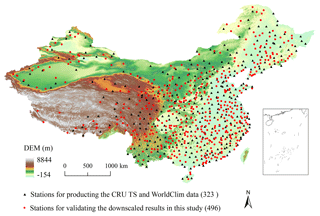
The monthly mean, maximum, and minimum air TMPs at 2 m as well as PRE were obtained for January 1901 to December 2017 with a spatial resolution of 30^′ from the CRU TS v4.02 dataset (http://www.cru.uea.ac.uk, last access: 25 April 2019) (Harris et al., 2014). Methodologies used by the CRU group to construct the 30^′ time series dataset are similar to the delta downscaling framework employed herein (see Sect. 3.1). First, more than 5000 weather stations were employed, and each station series was converted to anomalies by subtracting (for temperatures) or dividing (for precipitation) the 1961–1990 normal from the station's data. Then, the station anomaly time series data were linearly interpolated into 30^′ grids covering the global land surface. Finally, the grid anomaly time series data were transformed back to absolute monthly values using the 30^′ reference climatology dataset during 1961–1990. Specifically, the 30^′ reference climatology dataset used by the CRU group contained the climatology data for each month and was obtained from New et al. (1999). These climatology data were generated by a function considering the latitude, longitude, and elevation, based on 3615–19 800 weather stations located globally. Elevation data used in this climatology dataset had a spatial resolution of 30^′, which was a mean result of the global 5^′ digital elevation model. Specifically, elevation at each 30^′ grid was the mean of 36 grids of the 5^′ digital elevation model (New et al., 1999). Therefore, the CRU dataset could represent the orographic effects on climate variation at 30^′ spatial resolution. Compared with similar gridded products, the CRU dataset exhibited better performance. In addition, 323 weather stations across China were employed by the CRU group to generate CRU time series data (Harris et al., 2014) (Fig. 1).

Figure 2 Orographic statistical information at different gradients for China and weather stations used in this study.

2.2 WorldClim data

To downscale CRU TMPs and PRE time series data to higher spatial resolutions, we obtained four high-resolution reference datasets at spatial resolutions of 10^′, 5^′, 2.5^′, and 0.5^′ from WorldClim v2.0 (http://worldclim.org, last access: 25 April 2019) (Fick and Hijmans, 2017). The reference datasets comprised monthly averages of climatic variables (mean, maximum, and minimum air TMPs at 2 m as well as PRE) for 1970–2000, generated based on 9000–60 000 weather stations located globally using the thin-plate spline interpolation method. Thus, each climatic variable was associated with 12 climatology layers representing climatology data ranging from January to December. Remarkably, the interpolation considered co-variation with latitude, longitude, elevation, distance to the nearest coast, and three satellite-derived covariates: the maximum and minimum land surface temperature and cloud cover, obtained from the MODIS satellite platform. Thus, these reference data reflected orographic effects and observed climate information for each month. Moreover, cross-validation correlations indicated that these reference data exhibited good performance globally because of the introduction of satellite-derived covariates and distance to the nearest coast covariates. In addition, weather stations over China used in WorldClim were the same as those used in the CRU group (Fick and Hijmans, 2017) (Fig. 1). Herein, for an independent evaluation of the downscaled dataset, these weather stations were excluded.

2.3 Observations

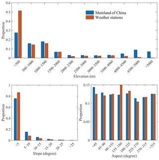
To evaluate the performance of the downscaling procedure, the observed long-term monthly TMPs (i.e., mean, maximum, minimum air TMPs at 2 m) and PRE variables across China were obtained from the National Meteorological Information Center of China (http://data.cma.cn/en). This dataset included observations from 496 national weather stations (Fig. 1) during 1951–2016. These stations were not considered in the generation of CRU time series and WorldClim data. Figure 2 shows the orographic statistical information (e.g., elevation, slope, and aspect) of China and the 496 independent weather stations. The results indicate that the proportion of independent weather stations in different orographic gradients almost corresponded to that in China, except for areas with elevations exceeding 4500 m, which indicated that these weather stations could represent climate variation over China and be used for validating the downscaled dataset. This exception is inevitable because of the observability, installation, and maintenance of weather stations over those areas. In addition, although China had few weather stations during 1901–1950, all of these stations were used to generate CRU time series data before 1950. Therefore, this study aimed to evaluate the downscaled dataset during 1951–2016 using 496 independent and representative stations.

3 Methods

3.1 Spatial downscaling

Delta downscaling was employed to generate monthly TMPs and PRE for the period of 1901–2017 at spatial resolutions of 10^′, 5^′, 2.5^′, and 0.5^′. The employed delta downscaling framework includes the following four steps (Peng et al., 2018).

First, a climatology dataset was constructed for each month and each climatic variable based on 30^′ CRU time series. In this step, the annual averages at each month for TMPs (i.e., mean, maximum, and minimum TMPs) and PRE variables were constructed based on CRU TMPs and PRE time series data. Specifically, the constructed climatology dataset had a spatial resolution of 30^′, which is the same as that of the CRU dataset. Moreover, to match the period of high-resolution reference datasets from WorldClim, the 30^′ climatology dataset was constructed for the period of 1970–2000. Thus, for each climatic variable, the dataset featured 12 climatology layers during 1970–2000 with a spatial resolution of 30^′.

Second, the 30^′ anomaly time series data were derived for each climatic variable based on the 30^′ CRU time series data and the constructed climatology dataset. In this step, the TMP anomaly time series data were calculated as the difference between the TMP time series and the TMP climatology data in the corresponding month, while the PRE anomaly time series data were calculated as the ratio of the PRE time series to the PRE climatology data in the corresponding month. The specific calculation equations are as follows:

$$\begin{array}{}\text{(1)}& {\displaystyle }& {\displaystyle }\text{An\_TMP}\left(\text{yr},m\right)=\mathrm{TMP}\left(\text{yr},m\right)-\text{CRUClim\_TMP}\left(m\right),\text{(2)}& {\displaystyle }& {\displaystyle }\text{An\_PRE}(\text{yr},m)=\mathrm{PRE}\left(\text{yr},m\right)/\text{CRUClim\_PRE}\left(m\right),\end{array}$$

where An_TMP(yr, m) and An_PRE(yr, m) are the anomalies for temperatures and precipitation, respectively; TMP(yr, m) and PRE(yr, m) are the absolute temperatures and precipitation values, respectively; CRUClim_TMP(m) and CRUClim_PRE(m) are the 30^′ climatology for temperatures and precipitation, respectively; and m and yr correspond to month (January–December) and year, respectively.

Third, the 30^′ anomaly time series dataset was spatially interpolated to a higher spatial resolution. In this step, the 30^′ anomaly grids at each time step are interpolated to four spatial resolutions (i.e., 10^′, 5^′, 2.5^′, and 0.5^′) to match the spatial resolutions of the reference datasets from WorldClim. Specifically, three interpolation methods are employed in this step, including bicubic, bilinear, and nearest-neighbor interpolation methods. This study compares the performances of these methods to select a reasonable interpolation approach.

Finally, the high-spatial-resolution anomaly time series dataset was transformed to an absolute climatic time series dataset based on the reference datasets from WorldClim at the corresponding spatial resolutions. In this step, the anomaly is undone at each time. Therefore, addition is used for TMPs, while multiplication is used for PRE. The specific calculation equations are as follows:

$$\begin{array}{}\text{(3)}& {\displaystyle }\begin{array}{rl}& \mathrm{TMP}\left(\text{yr},m,\text{res}\right)=\\ & \text{An\_TMP}\left(\text{yr},m,\text{res}\right)+\text{WorldClim\_TMP}\left(m,\text{res}\right),\end{array}\text{(4)}& {\displaystyle }\begin{array}{rl}& \mathrm{PRE}\left(\text{yr},m,\text{res}\right)=\\ & \mathrm{An}\mathrm{\_}\mathrm{PRE}\left(\text{yr},m,\text{res}\right)\times \text{WorldClim\_PRE}\left(m,\text{res}\right),\end{array}\end{array}$$

where m and yr are defined as above; res represents spatial resolution, i.e., 10^′, 5^′, 2.5^′, and 0.5^′; TMP(yr, m, res) and PRE(yr, m, res) are the absolute temperatures and precipitation values with a spatial resolution of res, respectively; An_TMP(yr, m, res) and An_PRE(yr, m, res) represent anomalies with a spatial resolution of res for temperatures and precipitation, respectively; and WorldClim_TMP(m, res) and WorldClim_PRE(m, res) represent climatology datasets from WorldClim at a spatial resolution of res for temperatures and precipitation, respectively.

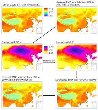
To visually present the downscaling processes, Fig. 3 illustrates the components and steps of the delta downscaling framework for obtaining the mean TMP by using the CRU 30^′ time series and WorldClim 0.5^′ climatology dataset. Specifically, to effectively interpolate the 30^′ anomaly time series dataset in China and conveniently implement the downscaling processes in the program code, downscaling was carried out in a rectangular region covering China (Fig. 3).

Figure 3 Schematic illustration of the delta spatial downscaling process using the mean TMP (TMP_m) in July 2017 obtained from the CRU data as an example.

3.2 Evaluation metrics

Four statistic indices were used to evaluate the original CRU and downscaled datasets, namely the Pearson's correlation coefficient (Cor), the mean absolute error (MAE), the root-mean-square error (RMSE), and the Nash–Sutcliffe efficiency coefficient (NSE). Cor was used to evaluate the correlation between original–downscaled and observed values, while MAE and RMSE assessed the bias between original–downscaled and observed values based on Eqs. (5) and (6). NSE was used to evaluate the performance of original and downscaled datasets based on Eq. (7), ranging from unity (best fit) to negative infinity (worst fit) (Nash and Sutcliffe, 1970).

$$\begin{array}{}\text{(5)}& {\displaystyle }& {\displaystyle }\mathrm{MAE}={\displaystyle \frac{\mathrm{1}}{n}}\sum _{i=\mathrm{1}}^n\left|P_i-O_i\right|\text{(6)}& {\displaystyle }& {\displaystyle }\mathrm{RMSE}=\sqrt{{\displaystyle \frac{\mathrm{1}}{n}}\sum _{i=\mathrm{1}}^n(P_i-O_i{)}^{\mathrm{2}}}\text{(7)}& {\displaystyle }& {\displaystyle }\mathrm{NSE}=\mathrm{1}-{\displaystyle \frac{\sum _{i=\mathrm{1}}^n{\left(P_i-O_i\right)}^{\mathrm{2}}}{\sum _{i=\mathrm{1}}^n{\left(O_i-\stackrel{\mathrm{‾}}{O}\right)}^{\mathrm{2}}}}\end{array}$$

Here P_i is the original or downscaled value in the time series, O_i is the observed value in the time series, and n is the number of months. Evaluations of the original CRU and downscaled datasets were carried out at each independent station to be mapped in geographic space, and the obtained results were averaged over all independent stations to compare the overall performances of original CRU and downscaled datasets.

In addition, WorldClim data at different spatial resolutions were evaluated using MAE and Cor indices, which were calculated according to the paired climatology values from WorldClim and observed data for the same geographic position. The sample size was the number of independent stations.

Table 1 Mean absolute errors between the observed and WorldClim climatology datasets at different spatial resolutions over independent weather stations for 1970–2000.

3.3 Evaluations of climatology and trends for the downscaled dataset

We also evaluated the climatology and trends for the 0.5^′ downscaled dataset by comparison with the 30^′ original CRU and observed datasets. The mean annual value of each climatic variable was used to represent climatology, and the annual trend was employed to indicate temporal variation. Specifically, the annual minimum TMP was the minimum value of monthly minimum TMPs in a year, the annual maximum TMP was the maximum value of the monthly maximum TMPs in a year, the annual mean TMP was the mean of the monthly mean TMPs in a year, and the annual PRE was the sum of the monthly precipitations in a year. For annual trend analysis, linear regression relationships between climatic variables and year were established to calculate the trend magnitude.

4 Results

4.1 Evaluation of WorldClim data at different spatial resolutions

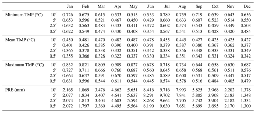
We evaluated the reliability of the WorldClim dataset based on observations from independent weather stations. Overall, the monthly climatology data with respect to temperature and precipitation exhibited a high performance for representing the monthly climatology data over China during 1970–2000, and the climatology dataset exhibited good performance at a higher spatial resolution. Specifically, the absolute errors of the WorldClim datasets decreased with increasing spatial resolution (Table 1), and correlations to observations increased with increasing spatial resolution (Table 2), especially for the 0.5^′ WorldClim dataset. Thus, the employed WorldClim datasets could be used as an input for the chosen downscaling processes.

Table 2 Correlation coefficients between the observed and WorldClim climatology datasets at different spatial resolutions over independent weather stations for 1970–2000.

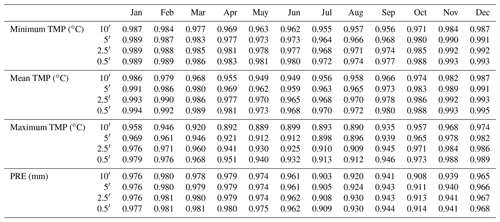
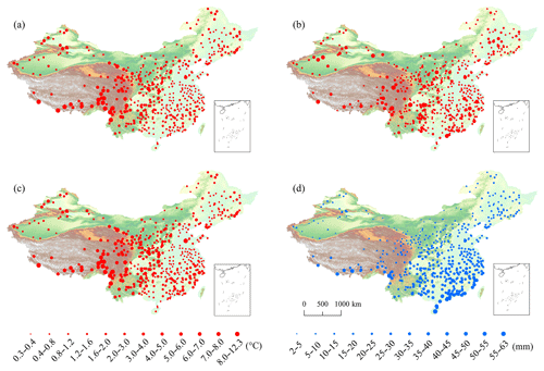
Figure 4 Spatial distribution of MAEs between the 30^′ original and observed TMPs–PRE from 1951 to 2016 at each independent weather station. Panels (a)–(d) show MAEs for the monthly minimum, mean, and maximum temperatures as well as the monthly precipitation, respectively.

Table 3 Statistical characterization of original–downscaled and observed monthly TMPs and PRE in the time series (1951–2016). The values shown here are the averaged evaluation results at all independent weather stations, with standard errors listed in Table S1.

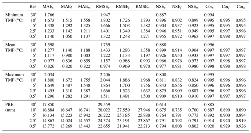
Notes: Res indicates spatial resolution. Subscripts c, l, and n indicate bicubic, bilinear, and nearest-neighbor interpolations, respectively. The original TMPs and PRE are the 30^′ CRU data and are directly compared with the observed data. Evaluations at 10^′, 5^′, 2.5^′, and 0.5^′ pertain to the downscaled datasets. MAE, RMSE, NSE, and Cor indicate the mean absolute error, root-mean-square error, Nash–Sutcliffe efficiency coefficient, and correlation coefficient, respectively.

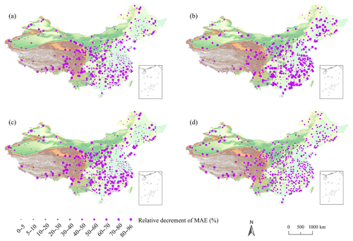
Figure 5 Relative decrement in MAEs from the 30^′ original datasets to 0.5^′ downscaled datasets generated using bilinear interpolation at each independent weather station. Panels (a)–(d) are the relative decrements in MAE for the monthly minimum, mean, and maximum temperatures as well as monthly precipitation, respectively.

4.2 Evaluation of original CRU temperatures and precipitation data

Prior to downscaling, we evaluated the performance of the original CRU time series dataset employed herein. Table 3 presents the averaged evaluation over independent weather stations, according to the evaluation result at each station for the original monthly TMP and PRE variables in the time series (1951–2016). The results show that (1) the dataset exhibited good performance for determining the original monthly TMPs and PRE values and (2) the performance of NSE and Cor indices for evaluating TMPs was better than that for evaluating PRE. Specifically, the MAEs of the minimum, mean, and maximum TMPs, as well as of PRE equaled 1.766, 1.598, 2.034 ^∘C, and 17.85 mm, respectively. The RMSEs of the minimum, mean, and maximum TMPs as well as of PRE equaled 1.947, 1.759, 2.206 ^∘C, and 29.559 mm, respectively. The NSEs of the minimum, mean, and maximum TMPs as well as of PRE equaled 0.887, 0.888, 0.8, and 0.614 respectively. The Cor's of the minimum, mean, and maximum TMPs as well as of PRE equaled 0.994, 0.996, 0.995, and 0.885, respectively.

Figure 4 maps the MAEs of the original TMP and PRE variables at each independent weather station, showing that (1) the original TMPs had larger biases in the northwest of China, especially at high-elevation regions and the Qinghai–Tibet Plateau, and (2) the original PRE had greater biases in the southern part of the Qinghai–Tibet Plateau and China.

Table 4 Comparison of the averaged climatology among the independent weather stations during 1951–2016, based on the 30^′ original datasets, the 0.5^′ datasets downscaled with the bilinear interpolation, and the observations.

Note all values are presented as mean ± standard error.

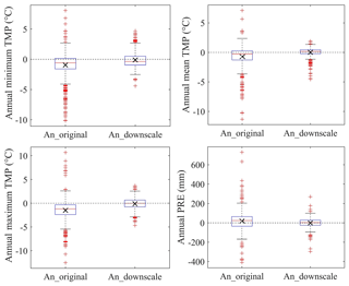
Figure 6 Box plots of climatology anomaly during 1951–2016 for 30^′ original and 0.5^′ downscaled datasets at independent weather stations. The climatology anomaly is equal to the bias from the original–downscaled to the observed values. Red lines in boxes show median values. Boxes indicate the inter-quantile range (25 %–75 %). Crosses (×) in boxes indicate the averages of all anomaly values. Horizontal dotted lines indicate zero values. An_original and An_downscale indicate climatology anomalies of the 30^′ original and 0.5^′ downscaled datasets, respectively. The 0.5^′ downscaled datasets were generated using bilinear interpolation in the delta downscaling framework.

4.3 Validation of downscaled CRU temperature and precipitation data

Table 3 presents the averaged evaluation over independent weather stations, based on the evaluation result at each station for the downscaled monthly TMPs and PRE in the time series (1951–2016) at different spatial resolutions. The results show that (1) compared with the original dataset, the downscaled dataset had lower MAEs and RMSEs and higher NSEs; (2) the increase in the spatial resolution of the WorldClim reference dataset from 10^′ to 0.5^′ resulted in a decrease in MAE and RMSE and an increase in NSE; (3) among the three interpolation methods employed in the delta downscaling framework, the bilinear interpolation method afforded downscaled data with the lowest MAEs and RMSEs as well as the highest NSEs at each spatial resolution; and (4) the performance of the delta downscaling framework was better for TMPs than for PRE. Specifically, compared with the original dataset, the MAE of the downscaled minimum TMP at 0.5^′ under the bilinear interpolation method decreased to 1.05 ^∘C (by 35.4 %), the RMSE decreased to 1.248 ^∘C (by 35.9 %), the NSE increased to 0.972 (by 9.6 %), and the Cor increased to 0.998 (by 0.4 %). For the mean TMP, the MAE of the downscaled data at 0.5^′ under the bilinear interpolation method decreased to 0.820 ^∘C (by 48.7 %), the RMSE decreased to 0.969 ^∘C (by 44.9 %), the NSE increased to 0.981 (by 10.5 %), and the Cor increased to 0.998 (by 0.2 %). For the maximum TMP, the MAE of the downscaled data at 0.5^′ under the bilinear interpolation method decreased to 1.282 ^∘C (by 37.0 %), the RMSE decreased to 1.491 ^∘C (by 32.4 %), the NSE increased to 0.91 (by 13.8 %), and the Cor increased to 0.997 (by 0.2 %). For PRE, the MAE of the downscaled data at 0.5^′ under the bilinear interpolation method decreased by 25.7 %, the RMSE decreased by 25.8 %, the NSE increased by 31.6 %, and the Cor increased by 5.0 %. Overall, the downscaled datasets had higher accuracy than the original CRU dataset, especially the 0.5^′ dataset downscaled using the bilinear interpolation method, which is, therefore, the new dataset proposed by this study.

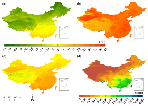
Figure 7 Spatial distributions of climatology data in the time period of 1901–2017 for TMPs and PRE over China, based on the 0.5^′ downscaled datasets generated using bilinear interpolation in the delta downscaling framework. Panels (a)–(d) correspond to the mean annual minimum, maximum, and mean temperatures as well as the mean annual precipitation, respectively.

Figure 5 maps the relative MAE decrement upon going from the 30^′ original dataset to the 0.5^′ dataset downscaled using the bilinear interpolation method. Compared with the MAEs of the original dataset, those of the downscaled dataset were lower for all independent stations, especially in the northwest of China and the Qinghai–Tibet Plateau.

4.4 Climatology of China based on the 0.5^′ downscaled dataset

Table 4 lists the averaged climatology data obtained from independent weather stations during 1951–2016 based on the 30^′ original dataset, the 0.5^′ dataset downscaled with bilinear interpolation, and the observations. The results indicate that the averaged climatology data for each climatic variable from the 0.5^′ downscaled data were closer to those from the observed data than to those from the 30^′ original data. Specifically, the averaged climatology differences between the 0.5^′ downscaled and observed data equaled −0.12 ^∘C for the annual minimum TMP, −0.12 ^∘C for the annual maximum TMP, 0.01 ^∘C for the annual mean TMP, and −0.5 mm for the annual total PRE.

To further illustrate the ability of the downscaled data to reflect climatology, we constructed box plots of the climatology anomaly during 1951–2016 for the 30^′ original and 0.5^′ downscaled datasets at independent weather stations, where the climatology anomaly is equal to the bias from the original–downscaled data to the observed values at each station (Fig. 6). The results show that the climatology anomaly from the 0.5^′ downscaled dataset more intensively embraced the zero value than that from the 30^′ original dataset, especially for median and mean values. These results imply that the 0.5^′ dataset downscaled with bilinear interpolation could better represent climatology in TMPs and PRE of China than the 30^′ original dataset.

In addition, we investigated climatology by using the 0.5^′ downscaled TMPs and PRE data generated by the bilinear interpolation method for 1901 to 2017 (Fig. 7). The mean annual minimum TMP for China ranged from −47.44 to 18.70 ^∘C, with an average of −13.19 ^∘C, and the lowest value corresponded to a location in the western part of the Qinghai–Tibet Plateau (Fig. 7a). The mean annual maximum TMP ranged from −17.53 to 42.23 ^∘C, with an average of 26.70 ^∘C, and the highest value was observed at a location in the Turpan Basin (Fig. 7b). The mean annual TMP ranged from −34.41 to 26.39 ^∘C, with an average of 6.18 ^∘C, and the lowest and highest values corresponded to locations in the western part of the Qinghai–Tibet Plateau and Hainan Island, respectively (Fig. 7c). The mean annual total PRE ranged from 3.2 to 4854.0 mm, with an average value of 564.4 mm, and the minimum and maximum values corresponded to locations in the northwestern part of the Qinghai–Tibet Plateau near the Tarim Basin and Taiwan Island, respectively (Fig. 7d). The climatology data for the three TMPs varied with topography and notably decreased with orographic uplift. The climatology data for PRE decreased upon going from the southeastern coastal region to the northwestern region. These results almost fit the orographic and coastal effects on the climatology of China.

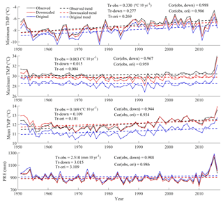
Figure 8 Temporal variations in annual TMPs and PRE over China during 1951–2016 based on the 0.5^′ downscaled datasets with bilinear interpolation, 30^′ original datasets, and observed datasets. Tr-obs, Tr-down, and Tr-ori indicate the annual trends calculated using the observed, 0.5^′ downscaled, and 30^′ original datasets, respectively. Cor(obs, down) indicates the correlation coefficients of the annual values from observed and 0.5^′ downscaled data, while Cor(obs, ori) indicates the correlation coefficients of the annual values from the observed and 30^′ original data.

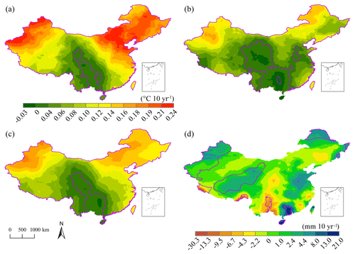
Figure 9 Spatial patterns of the annual trends in TMPs and PRE from 1901 to 2017 across China obtained using the 0.5^′ downscaled data with bilinear interpolation. Panels (a)–(d) correspond to the annual minimum, maximum, and mean TMPs as well as the annual PRE, respectively. Purple zones indicate locations where trends are significant at the 95 % confidence level.

4.5 Trends of the annual temperatures and precipitation in China

Figure 8 maps the annual trends in TMPs and PRE over China during 1951–2016 based on the 0.5^′ downscaled dataset with bilinear interpolation, the 30^′ original dataset, and the observed dataset. The results show that (1) the annual values of TMPs and PRE in the 0.5^′ downscaled dataset were closer to observations than the original values in the time series, (2) the annual trends from the 0.5^′ downscaled dataset were closer to the observed trends than to those from the 30^′ original data, and (3) the temporal correlations between the 0.5^′ downscaled and observed data were slightly better than those between the 30^′ original and observed data, although the latter were sufficiently good. Furthermore, the annual trends in the TMPs in the 0.5^′ downscaled dataset were underestimated (by 0.053, 0.048, and 0.06 ^∘C 10 yr⁻¹ for the minimum, maximum, and mean TMPs), while those in the PRE in the 0.5^′ downscaled dataset were overestimated (by 0.505 mm 10 yr⁻¹). Overall, the 0.5^′ downscaled and observed data had minor differences with respect to annual trends and high temporal correlations, and thus it was concluded that the 0.5^′ downscaled dataset can be used to represent temporal variations and trends in TMPs and PRE across China.

In addition, we investigated the spatial patterns of annual trends in TMPs and PRE from 1901 to 2017 across China by using the 0.5^′ dataset downscaled with bilinear interpolation (Fig. 9). A 95 % significance level was selected to represent the significance of the trend for each climatic variable. The annual minimum TMP exhibited a significant upward trend from 0.018 to 0.240 ^∘C 10 yr⁻¹, with an average of 0.131 ^∘C 10 yr⁻¹, over areas accounting for approximately 94.17 % of the total land area of China (Fig. 9a). The annual maximum TMP exhibited a significant upward trend from 0.016 to 0.171 ^∘C 10 yr⁻¹, with an average of 0.081 ^∘C 10 yr⁻¹, over areas accounting for approximately 80.85 % of the total land area of China (Fig. 9b). Meanwhile, the annual maximum TMP exhibited a significant downward trend from 0.019 to 0.034 ^∘C 10 yr⁻¹, with an average of 0.027 ^∘C 10 yr⁻¹, in areas accounting for only ∼ 0.33 % of the land area of China (Fig. 9b). The annual mean TMP exhibited a significant upward trend from 0.017 to 0.189 ^∘C 10 yr⁻¹, with an average of 0.104 ^∘C 10 yr⁻¹, over areas accounting for approximately 90.92 % of the total land area of China (Fig. 9c). The annual PRE exhibited a significant upward trend from 0.11 to 21.206 mm 10 yr⁻¹, with an average of 3.306 mm 10 yr⁻¹, over areas accounting for ∼ 22.02 % of the total land area of China (Fig. 9d). Meanwhile, the annual PRE exhibited a significant downward trend from 0.13 to 30.321 mm 10 yr⁻¹, with an average of 7.147 mm 10 yr⁻¹, over areas accounting for only ∼ 2.01 % of China (Fig. 9d). Therefore, the 0.5^′ data downscaled with the bilinear interpolation proposed herein were concluded to represent the detailed spatial variability of trends in TMPs and PRE across China well.

5 Data availability

The 0.5^′ downscaled dataset with bilinear interpolation developed in this study has been published in Network Common Data Form (NetCDF) at https://doi.org/10.5281/zenodo.3114194 for precipitation (Peng, 2019a) and https://doi.org/10.5281/zenodo.3185722 for air temperatures at 2 m (Peng, 2019b). The dataset includes the monthly minimum, maximum, and mean temperatures, as well as the monthly total precipitation from January 1901 to December 2017. Because of the availability of original CRU data and the spatial resolution of the reference climatology data, the data cover most of the land area of China, with a geographic range of 18.2–53.5^∘ N and 73.5–135.0^∘ E. The total number of grids is 13 808 747. To reduce the size of the NetCDF file, the data for each climatic variable are divided into intervals of 3 years. TMPs and PRE are expressed to precision of 0.1 ^∘C and 0.1 mm, respectively, and stored using the int16 format. Thus, each file contains 36 months of data and requires 2.42 GB of storage space. This file size is convenient for processing by modern computers, and subparagraph storage in the time series can satisfy the need for quick data access for a specific period. Each file name indicates the data contained in the file, in the format “data type”_“beginning year”_“ending year”.nc. For example, the file named tmn_1901_1903.nc contains minimum temperature data from 1901 to 1903. The total number of NetCDF files is 156, and the total size of the dataset in nc format is approximately 378 GB. After compression in zip format, the size of each file is approximately 300 MB, which translates into a total dataset size of 47.8 GB. This dataset will be updated yearly, as the CRU TS dataset is also updated yearly, and new data will become available for download from the website identified above.

The monthly TMPs and PRE data in the 30^′ original dataset from 1901 to 2017 were obtained from the CRU TS v4.02 dataset (http://www.cru.uea.ac.uk/data, last access: 25 April 2019). The high-resolution reference data at spatial resolutions of 10^′, 5^′, 2.5^′, and 0.5^′ for TMPs and PRE were supported by WorldClim v2.0 (http://worldclim.org/version2, last access: 25 April 2019). The observed monthly meteorological data from the 496 weather stations across China were provided by the National Meteorological Information Center of China (http://data.cma.cn/en, last access: 25 April 2019).

6 Discussion, limitations, and recommendations

Although the original CRU dataset with a 30^′ spatial resolution was not evaluated as being poor, the 0.5^′ dataset downscaled with bilinear interpolation was evaluated as being better, with deviations decreasing by 35.4 %–48.7 % for TMPs and by 25.7 % for PRE relative to the original CRU dataset (Table 3). Thus, the original CRU dataset needs to be corrected. Many factors contribute to these deviations, e.g., observational errors, sample size, and operator errors in gathering the original CRU data. However, little work has been done to address this issue. Previous studies indicated that topographic information (e.g., elevation, location, slope, and aspect) may be the key factor for correcting deviations, especially in mountainous areas (Gao et al., 2018, 2017; Peng et al., 2014). Therefore, a high-resolution reference climatology dataset containing detailed topographic information, as well as the effects of distance to the nearest coast and satellite-derived covariates, was used in this study to downscale the 30^′ original CRU dataset to a 0.5^′ dataset comprising monthly TMPs and PRE from January 1901 to December 2017 across China, which has a low density of weather stations in mountainous areas. To the best of our knowledge, this 0.5^′ downscaled dataset is the first dataset (version 1.0) developed with such a high spatiotemporal resolution over such a long time period for China.

Compared with the original CRU dataset, the downscaled dataset exhibited smaller deviations and higher spatial resolutions, which suggested that the delta downscaling framework can be used to downscale and correct low-spatial-resolution climate data. This should be attributed to the introduction of the high-spatial-resolution WorldClim data because the reference climatology dataset with higher spatial resolution could produce more accurate downscaled data with a higher spatial resolution (Tables 1–3). Remarkably, because of the introduction of the averaged 30^′ elevation information in the original CRU data, these data weaken the representation of TMPs and PRE on the actual land surface, especially in regions with complex terrain. Moreover, the original CRU dataset was evaluated at weather stations, which are often located in valleys near counties or cities. Thus, the TMPs and PRE from the CRU dataset exhibited lower and higher values than those from the observations, respectively (Table 4 and Fig. 6). However, the deviations decreased to a certain extent in the 0.5^′ downscaled dataset (Table 4 and Fig. 6). Even so, the delta downscaling processes did not considerably improve the temporal correlations between 0.5^′ downscaled and observed data (Table 3). This could be attributed to the fact that the delta downscaling processes focus on correcting deviations and downscaling the spatial resolution, using the 12 climatology layers from the WorldClim dataset. In geographical space, the corrections are evident, especially in the northwest of China and the Qinghai–Tibet Plateau (Fig. 5), which should result from the introduction of orographic effects, distance to the nearest coast, and effects of satellite-derived covariates in the WorldClim dataset.

The 0.5^′ downscaled TMP and PRE dataset with bilinear interpolation captures the detailed climatology of the whole of China very well (Fig. 7), accurately representing climate characteristics such as the minimum TMP at high elevations (e.g., the Qinghai–Tibet Plateau), the maximum TMP at low elevations (e.g., the Turpan Basin), and heavy PRE in marine areas (e.g., Taiwan Island). The biases of climatology data were only −0.12 ^∘C for the minimum TMP, −0.12 ^∘C for the maximum TMP, 0.01 ^∘C for the mean TMP, and −0.5 mm for PRE (Table 4). Furthermore, the climatology anomaly at each weather station from the 0.5^′ downscaled dataset is closer to zero than that from the 30^′ original dataset (Fig. 6). The 0.5^′ dataset downscaled with bilinear interpolation also represents detailed annual trends in climatic variables over China very well (Fig. 9), precisely representing the trends and their significance levels over the geographic space, such as significant increases and decreases in the maximum TMP and PRE. In general, compared with the 30^′ original dataset, this dataset captures the annual trends very well (Fig. 8); the 0.5^′ downscaled and observed data exhibit high temporal correlations and minor differences in annual trends (Fig. 8). Therefore, the 0.5^′ dataset downscaled with bilinear interpolation can be used to successfully assess climate change and its spatial effects across China.

As mentioned previously, the accuracy of the reference climatology dataset largely determines its quality. Herein, the reference climatology dataset from WorldClim was adopted. Although our evaluation indicated that the quality of the dataset is very good, a gap between the dataset and observed data was observed. We think that a new and better reference climatology dataset should be generated using the observed data gathered across China. However, the current release of public climate data over China is insufficient to construct a reference climatology dataset better than that available from WorldClim. In our future research, we plan to collect more public and private climate data to construct a better reference climatology dataset and then generate a more accurate downscaled dataset for China.

Another limitation is the difficulty of validating the new dataset before 1950. Although China had several weather stations with data collected starting from 1901, all of them have been used to generate the CRU time series (Harris et al., 2014). Therefore, we cannot verify the quality of data before 1950 because of data unavailability. However, the downscaling procedure only used data from original CRU and WorldClim datasets as inputs, and thus the quality of the new dataset throughout the period of 1901–2017 depended on input quality. Evaluations showed that the qualities of the original CRU and WorldClim datasets are overall satisfactory and that the downscaling procedure can further improve the quality of the original CRU dataset as well as enhance its spatial resolution. The usage of some evaluation indices may have defects and should be clarified in this study. The indices used herein can be classified into two groups, one based on the sums of squared errors (i.e., RMSE and NSE) and the other based on the sums of error magnitudes (i.e., MAE). The sums of the squared errors are influenced by three independent variables, namely the mean of individual error magnitudes, variability among error magnitudes, and the number of observations or domains of integration (Willmott et al., 2009). Willmott and Matsuura (2005) recommended MAE as an evaluation criterion for estimations. However, this study adopted the CRU time series dataset as a unique original dataset and observations from 496 weather stations as a unique evaluation dataset. Thus, the variations in RMSE or NSE in different cases were only influenced by the mean of individual error magnitudes, which were introduced by different spatial resolutions and interpolation methods. Thus, RMSE and NSE indices satisfied the evaluation criteria of this study. Further, the evaluation indices were mainly used to compare the performance of the downscaled and original datasets. Therefore, the usage of these indices in this study is reasonable.

In addition, because of the limitations associated with the computational resources and the resolutions of reference climatology and the original CRU dataset, the resolution of the new dataset is limited to monthly and 0.5^′ (∼ 1 km) grid spacing. However, the current dataset (approximately 378 GB) is very large to process and store. The computational resources and disk space required for the dataset will increase exponentially with increasing spatiotemporal resolution (Gao et al., 2018). For such a large amount of data, storage and extraction are not convenient, and supercomputers as well as parallel computing will be required for work with larger datasets in the future. Another limitation is that the current dataset only includes historical climate data. Many GCM products have been released, but their coarse spatial resolution and low accuracy prevent detailed projections of future climate trends and their effects on local scales, which are urgently required for planning local strategies of coping with the negative effects of future climate changes. The delta spatial downscaling procedure has been employed to generate future climate data at high resolutions for some areas (Peng et al., 2017).

The issues associated with computational resources, validation, and a reasonable reference climatology must be addressed to generate high-resolution climate data for China in the future. Higher-resolution data, more validation, and a better reference climatology for historical and future climate data (version 2.0) are concerns to be addressed in future research.