the Creative Commons Attribution 4.0 License.
the Creative Commons Attribution 4.0 License.
 | 06 Feb 2019
Multi-source global wetland maps combining surface water imagery and groundwater constraints
Ardalan Tootchi
Anne Jost
Agnès Ducharne
Many maps of open water and wetlands have been developed based on three main methods: (i) compiling national and regional wetland surveys, (ii) identifying inundated areas via satellite imagery and (iii) delineating wetlands as shallow water table areas based on groundwater modeling. However, the resulting global wetland extents vary from 3 % to 21 % of the land surface area because of inconsistencies in wetland definitions and limitations in observation or modeling systems. To reconcile these differences, we propose composite wetland (CW) maps, combining two classes of wetlands: (1) regularly flooded wetlands (RFWs) obtained by overlapping selected open-water and inundation datasets; and (2) groundwater-driven wetlands (GDWs) derived from groundwater modeling (either direct or simplified using several variants of the topographic index). Wetlands are statically defined as areas with persistent near-saturated soil surfaces because of regular flooding or shallow groundwater, disregarding most human alterations (potential wetlands). Seven CW maps were generated at 15 arcsec resolution (ca. 500 m at the Equator) using geographic information system (GIS) tools and by combining one RFW and different GDW maps. To validate this approach, these CW maps were compared with existing wetland datasets at the global and regional scales. The spatial patterns were decently captured, but the wetland extents were difficult to assess compared to the dispersion of the validation datasets. Compared with the only regional dataset encompassing both GDWs and RFWs, over France, the CW maps performed well and better than all other considered global wetland datasets. Two CW maps, showing the best overall match with the available evaluation datasets, were eventually selected. These maps provided global wetland extents of 27.5 and 29 million km2, i.e., 21.1 % and 21.6 % of the global land area, which are among the highest values in the literature and are in line with recent estimates also recognizing the contribution of GDWs. This wetland class covers 15 % of the global land area compared with 9.7 % for RFW (with an overlap of ca. 3.4 %), including wetlands under canopy and/or cloud cover, leading to high wetland densities in the tropics and small scattered wetlands that cover less than 5 % of land but are highly important for hydrological and ecological functioning in temperate to arid areas. By distinguishing the RFWs and GDWs based globally on uniform principles, the proposed dataset might be useful for large-scale land surface modeling (hydrological, ecological and biogeochemical modeling) and environmental planning. The dataset consisting of the two selected CW maps and the contributing GDW and RFW maps is available from PANGAEA at https://doi.org/10.1594/PANGAEA.892657 (Tootchi et al., 2018).
- Article
(11528 KB) - Full-text XML
-
Supplement
(1421 KB) - BibTeX
- EndNote


Table 1Summary of water body, wetland and related proxy maps and datasets from the literature. The wet fractions indicated in % in the last column are those indicated in the reference paper or data description for each study.

a Percentages are those from the corresponding journal article or book. If no mention of percentage coverage exists, the value is calculated by dividing the wetland area by the land surface area excluding Antarctica, glaciated Greenland and lakes. b Excluding Caspian Sea and large lakes. c Excluding Antarctica, glaciated Greenland, lakes and Caspian Sea. Additionally the range in GLWD is different based on interpretation of fractional wetlands. d Excluding large water bodies. e Including the Caspian Sea.
Wetlands are valuable ecosystems with a key role in carbon, water and energy cycles (Matthews and Fung, 1987; Richey et al., 2002; Repo et al., 2007; Ringeval et al., 2012). Water retention in wetlands leads to lower and delayed runoff peaks, higher base flows and evapotranspiration, which directly influence climate (Bierkens and van den Hurk, 2007; Lin et al., 2016). Wetlands also serve to purify pollution from natural and human sources, thus maintaining clean and sustainable water for ecosystems (Billen and Garnier, 1999; Dhote and Dixit, 2009; Curie et al., 2011; Passy et al., 2012). Despite their widely recognized importance, no consensus exists on wetland definitions and their respective areal extents among the reviewed literature (Table 1). Based on several definitions, the extents range from regions with relatively shallow water tables (National Research Council, 1995; Kutcher, 2008; Ramsar, 2009) to areas with permanent inundation such as lakes (lacustrine wetlands) with depths of several meters. The reasons for this ambiguity are a diversity of scientific points of views as well as the complexity of classification in transitional land features and temporally varying land features under human influences (Mialon et al., 2005; Papa et al., 2010; Ringeval et al., 2011; Sterling et al., 2013; Hu et al., 2017; Mizuochi et al., 2017).
The first global wetland maps were developed based on a compilation of regional archives and estimates. Matthews and Fung (1987) developed a 1∘ resolution wetland map based on vegetation, soil properties and inundation fractions that covered ca. 4 % of the land. Finlayson et al. (1999) based their estimates on surveys and the Ramsar global inventory in which wetlands cover 9.7 % of the land area. Later, the Global Lakes and Wetlands Database (GLWD) was developed at 30 arcsec resolution (∼1 km at the Equator) by compiling several national and regional wetland maps with a global cover of 6.9 % of the land area, excluding Antarctica and glaciated lands (Lehner and Döll, 2004). Because satellite imagery permits homogeneous observation of land characteristics, this method has been favored for mapping of water-related features in recent decades. Satellite imagery at visible wavelengths reports that 1.6 % to 2.3 % of Earth's land is permanently under water (Verpoorter et al., 2014; Feng et al., 2015; Yamazaki et al., 2015; Pekel et al., 2016), but with large disagreements (Nakaegawa, 2012), and inundations under densely vegetated and clouded areas are often missed (Lang and McCarty, 2009). Longer wavelengths in the microwave band (e.g., L and C bands) penetrate better through the cloud and vegetation layer and supply dynamic observations of inundated zones, usually with a trade-off between high resolution with a low revisit rate or domain extent (Li and Chen, 2005; Hess et al., 2015) and coarse resolution with a high revisit rate up to global coverage (Prigent et al., 2007; Papa et al., 2010; Schroeder et al., 2015; Parrens et al., 2017). Recent progress has been achieved by downscaling or correcting the latter products using higher-resolution information. Fluet-Chouinard et al. (2015) developed the global inundation product GIEMS-D15 by downscaling the 0.25∘ multi-satellite wetland fractions of Prigent et al. (2007) using 15 arcsec topography, with a global long-term maximum inundation fraction of 13 %. Poulter et al. (2017) corrected the wetland fractions of the surface water microwave product series (SWAMPS; Schroeder et al., 2015) by merging them with those obtained at 30 arcsec from GLWD.
However, regardless of the wavelengths, wetlands derived from satellite imagery almost always represent inundated areas and overlook other types of wetlands where soil moisture is high but the surface is not inundated (Maxwell and Kollet, 2008; Lo and Famiglietti, 2011; Wang et al., 2018). The method most frequently used to delineate these wetlands is water table depth (WTD) modeling. Direct groundwater (GW) modeling (e.g., Miguez-Macho and Fan, 2012) requires in-depth knowledge of the physics of water movement, topography at a sufficiently high resolution, climate variables, subsurface characteristics and observational constraints (Fan et al., 2013; de Graaf et al., 2015). Simplified GW models based on the topographic index (TI) of TOPMODEL (Beven and Kirkby, 1979) require less extensive input, and they have also been used to map wetlands (e.g., Gedney and Cox, 2003). Using the topography, the TI can be calculated as follows:
where a(m) is the drainage area per unit contour length and tan (β) is the local slope at the desired pixel. The TI is often presented as a wetness index (Wolock and McCabe, 1995; Sørensen et al., 2006) because high values are found over flat regions, with large drainage areas corresponding to a high propensity for saturation. Other environmental characteristics such as climate and soil or underground properties can also be used in the TI formulation to detect wetlands in areas where topography is not the primary driver of the water budget, such as wetlands in uplands and over clayey soils or thin active layers in the permafrost region (e.g., Saulnier et al., 1997; Mérot et al., 2003; Hu et al., 2017).
A major challenge in the identification of wetlands through GW modeling is the definition of thresholds on TI or WTD for separation of wetland from non-wetland areas. The thresholds are often calibrated to reproduce the extent of documented wetlands in a certain region and are subsequently extrapolated for larger domains. This strategy was proven successful at the basin scale (e.g., Curie et al., 2007), but it has been shown to be ineffective at larger scales because it is not possible to uniquely link TI values to soil saturation levels across different landforms and climates (Marthews et al., 2015). Hu et al. (2017) produced a global wetland map by calibrating TI thresholds for every large basin of the world based on land cover maps, as pioneered over France due to independent TI threshold calibration in 22 hydro-ecoregions using soil type datasets (Berthier et al., 2014). Uniform WTD thresholds (0 cm for inundated areas and 25 cm for wetlands) are applied in the only example (to the best of our knowledge) of direct global GW modeling for wetland delineation (Fan and Miguez-Macho, 2011; Fan et al., 2013). All these datasets based on GW modeling estimate the wetland fraction as being much higher than those based on inventories and satellite imagery (Hu et al., 2017: 22.6 %, Fan et al., 2013: 15 % of the land surface area). It must be emphasized that adjustment of wetland thresholds, both for directly modeled WTD and TI, always implies subjective choices and can result in over- or underestimation of wetland extents or unrealistic wetland distribution patterns.
The scientific objective of the current work is to develop a comprehensive global wetland dataset based on a unique and applicable wetland definition for use in hydrological and land surface modeling. Based on the above analysis, our rationale is that inundated and groundwater-driven wetlands must both be considered to realistically capture the wetland patterns and extents. This approach leads to a definition of wetlands as areas that are persistently saturated or near-saturated because they are regularly subject to inundation or shallow water tables. This definition is focused on hydrological functioning, and is not restricted to areas with typical wetland vegetation. In this context, although inundated areas and zones with shallow groundwater partially overlap and share similar environmental properties, they cannot be detected using a single method. Thus, we rely on data fusion methods, which have proven advantageous in developing high-quality products by merging properties from various datasets (Fritz and See, 2005; Jung et al., 2006; Schepaschenko et al., 2011; Pérez-Hoyos et al., 2012; Tuanmu and Jetz, 2014), including wetland mapping (Ozesmi and Bauer, 2002; Friedl et al., 2010; Poulter et al., 2017). In this framework, we tested several composite wetland (CW) maps, all constructed at 15 arcsec resolution, by merging two complementary classes of wetlands: (1) regularly flooded wetlands (RFWs), where surface water can be detected at least once a year through satellite imagery, and (2) groundwater-driven wetlands (GDWs) based on groundwater modeling.
The main assumptions underlying the composite wetland maps are detailed in Sect. 2, together with the datasets involved. Subsequently, Sect. 3 sequentially presents the construction of the RFW, GDW and CW maps, with preliminary analyses of their features and uncertainties. In Sect. 4, we compare the CW maps with several validation wetland datasets, globally and in several areas with contrasting climates and wetland fractions, to show that the combination of RFWs and GDWs provides a consistent wetland description throughout the globe. This comparison allows us to select two CW maps with better overall performances, used to discuss the role of GDWs in Sect. 5. Finally, the availability and potential applications of the composite maps are presented in Sect. 6, while Sect. 7 summarizes the advantages and limitations of the approach and gives perspectives on future developments.
2.1 Mapping strategy and requirements
Based on the inclusive assumptions for wetland mapping in this study, we use GIS tools to construct several composite wetland maps as the overlap (union) of the following:
-
one RFW map developed by overlapping three surface water and inundation datasets derived from satellite imagery in an attempt to fill the observation gaps (Sect. 3.1);
-
one GDW map out of seven, all derived from GW modeling (either direct or simplified based on several TI versions) and meant to sample the uncertainty of the GDW contribution (Sect. 3.2).
Table 2Layers of wetlands constructed in the paper, their definitions and the subsections in which they are explained. The total land area for wetland percentages excludes lakes, Antarctica and the Greenland ice sheet.
In this process, many layers were developed and are summarized in Table 2 and detailed in Sect. 3. The map and methods to exclude lakes from all layers are explained in Sect. 2.2. Input datasets to RFWs and GDWs are presented in Sect. 2.3 and 2.4, respectively, and several independent validation datasets, global and regional, are presented in Sect. 2.5. It should be noted that in the remainder of this paper, the wetland percentages of the land surface area always exclude lakes (Sect. 2.2), the Caspian Sea, the Greenland ice sheet and Antarctica (unless otherwise mentioned). For this reason, these percentages and areas might be different from those shown in Table 1, which are indicated for each original paper or data description.
2.2 Lakes
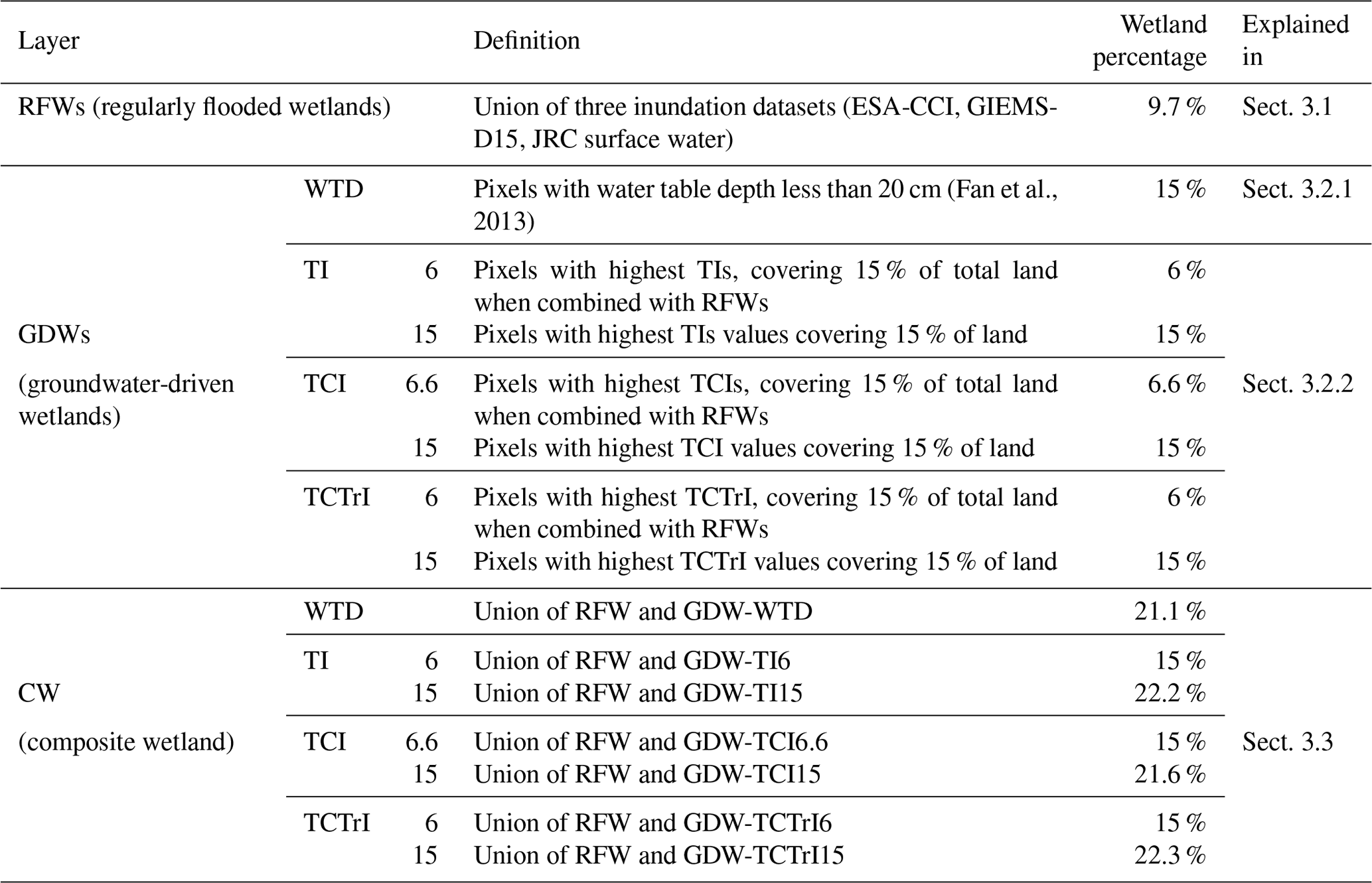
To distinguish large permanent lakes and reservoirs from wetlands, we used the HydroLAKES database (Messager et al., 2016), which was developed by compiling national, regional and global datasets (Fig. 1a). This database consists of more than 1.4 million individual polygons for lakes with a surface area of at least 10 ha, covering 1.8 % of the land surface area. It also classifies artificial dam reservoirs which amount to 300×103 km2 (Messager et al., 2016). The lakes' extent in HydroLAKES is smaller than in other recent databases that account for smaller water bodies: 2.5 % in G3WBM (Yamazaki et al., 2015) for water bodies above 0.8 ha and 3.5 % in GLOWABO (Verpoorter et al., 2014) for those above 0.2 ha. These two datasets do not differentiate lakes from other surface water elements, and using them as a mask would lead to the exclusion of shallow inundated portions of wetlands (e.g., Indonesian mangroves or Ganges floodplains). It must also be noted that the small water bodies tend to be overlooked after dominant resampling to 15 arcsec resolution (Sect. 2.6), unless they are sufficiently numerous in a pixel. Therefore, the lake mask covers 1.7 % of the land area compared with 1.8 % in the original HydroLAKES database. This map also shows that most of the lakes are located in the northern boreal zones (more than 60 % of lakes area are located north of 50∘ N), in agreement with the other lake databases.
2.3 Input to RFW map: inundation datasets
2.3.1 ESA-CCI land cover
This dataset succeeds the GlobCover dataset based on the data from the MERIS sensor (onboard ENVISAT) collected at high resolution for surface water detection, together with the SPOT-VEGETATION time series (Herold et al., 2015) to aid in distinguishing wetlands from other vegetation covers. Global land cover maps at approximately 300 m (10 arcsec) resolution deliver data for three 5-year periods (1998–2002, 2003–2007 and 2008–2012). The extents of water bodies slightly changed between the first 5-year period and the third one (such as shrinking of the Aral Sea area by more than 55 %), but the extent of wetland classes (permanent wetlands and flooded vegetation classes) did not change significantly (the variation in wetland classes throughout these periods is less than 3 % of the total wetlands area). We acquired the last epoch data to represent the current state of wetlands (Fig. 1b). In ESA-CCI, wetlands are mixed classes of flooded areas with tree covers, shrubs or herbaceous covers plus inland water bodies, covering 3 % of the Earth land surface overall.
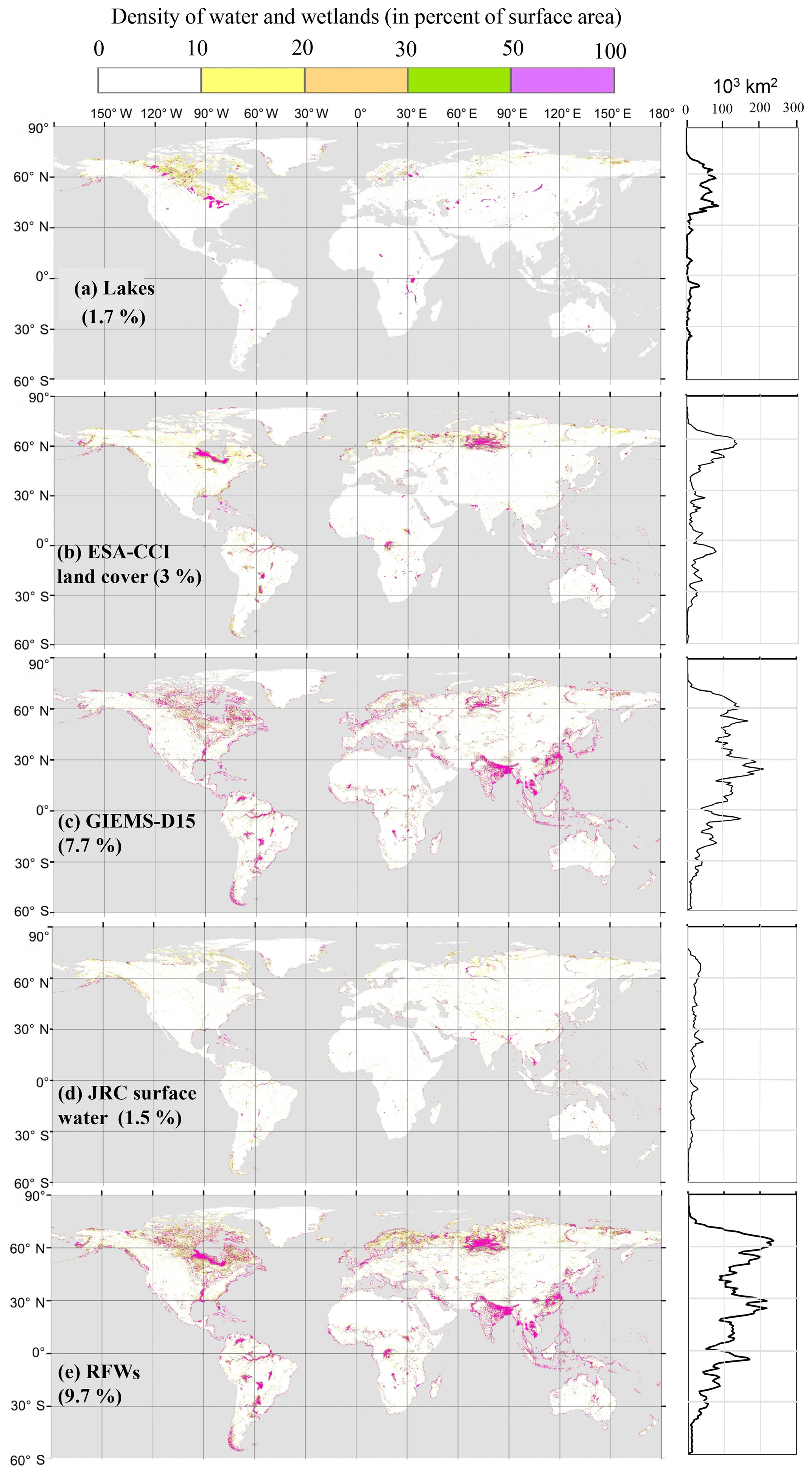
Figure 1Density of lakes, regularly flooded wetlands and components of the latter (percent area in 3 arcmin grid cells). For zonal wetland area distributions (right-hand charts), the area covered by wetlands in each 1∘ latitude band is displayed.
2.3.2 GIEMS-D15 (Fluet-Chouinard et al., 2015)
Prigent et al. (2007) used multi-sensor satellite data, including passive and active microwave measurements, together with visible and near-infrared reflectance to map the monthly mean inundated fractions at 0.25∘ resolution for a 12-year period (1993–2004). This dataset (GIEMS) gives the minimum and maximum extent of the inundated area (including wetlands, rivers, small lakes and irrigated rice). Fluet-Chouinard et al. (2015) used the GLC2000 land cover map (Bartholomé and Belward, 2005) to train a downscaling model for GIEMS at 15 arcsec resolution based on the HydroSHEDS digital elevation model (Lehner et al., 2008) and developed three static datasets for mean annual minimum, mean annual maximum and long-term maximum extent of the inundated areas (covering 3.9 %, 7.7 % and 10.3 % of the land surface area, respectively). In this study, we assumed that the mean annual maximum extent was the best representative measure for wetlands. In the following, GIEMS-D15 always indicates the mean annual maximum of GIEMS-D15 (Fig. 1c). Higher-resolution (3 arcsec) downscaling of GIEMS has been recently developed (Aires et al., 2017), but we overlooked this source because we focused our study on 15 arcsec resolution.
2.3.3 JRC surface water (Pekel et al., 2016)
The JRC surface water products are a set of high-resolution maps (1 arcsec, ∼30 m) for permanent water and also for seasonal and ephemeral water bodies. These products are based on analysis of Landsat satellite images (Wulder et al., 2016) over a period of 32 years (1984–2015). Each pixel was classified as open water, land or a nonvalid observation. Open water is defined as any pixel with standing water, including fresh and saltwater. The study also quantifies the conversions, mostly referring to changes in state (lost or gained water extents, conversions from seasonal to permanent, etc.) during the observation period. In this study, we used the maximum surface water extent, which consists of all pixels that were under water at least once during the entire period, covering almost 1.5 % of the Earth land surface area (Fig. 1d).
2.4 Input to GDW maps
2.4.1 Water table depth estimates (Fan et al., 2013)
Fan et al. (2013) performed global GW modeling to estimate the water table depth at 1 km resolution. This model assumes a steady flow, and lateral water fluxes are calculated using Darcy's law and the Dupuit–Forchheimer approximation for 2-D flow. Elevation is described at 30 arcsec resolution (by HydroSHEDS south of 60∘ N and otherwise by ASTER/NASA-JPL), and the recharge rates were modeled at 0.5∘ resolution using the WaterGAP model (Döll and Fiedler, 2008) based on contemporary meteorological forcing (1979–2007). To estimate subsurface transmissivity, the soil hydraulic conductivities were derived from the global Food and Agriculture Organization (FAO) digital soil maps (5 arcmin resolution) and US Department of Agriculture (USDA) soil maps over the United States (30 arcsec resolution) and subsequently assumed to decay exponentially with depth from the thin soil layer (2 m) down as a function of the local topographic slope. The decay factor is also adjusted for the permafrost region using an additional thermic factor (smaller transmissivity in permafrost areas). The modeled WTD was compared to observations available to the authors (more than 1 million observations, with 80 % of them located in North America). The resulting dataset suggests vast areas with a shallow water table over the tropics, along the coastal zones and in boreal areas of North America and Asia (almost 15 % of the land area for WTD ≤20 cm).
2.4.2 Three maps of topographic wetness indices
Flat downstream areas display a marked propensity to be saturated, which explains the wide use of topographic indices to delineate wetlands. Here, we use the global map of TI produced by Marthews et al. (2015) at 15 arcsec resolution. It relies on the original formulation of Beven and Kirkby (1979), as in Eq. (1), and on two global high-resolution digital elevation models (DEMs), viz. HydroSHEDS (Lehner et al., 2008) and Hydro1k (US Geological Survey, 2000) at 15 and 30 arcsec resolution, respectively. Hydro1k is used to fill the lack of information in HydroSHEDS north of 60∘ N, which is outside of the SRTM (Shuttle Radar Topography Mission) coverage. Because index values depend on pixel size, which varies with latitude, those researchers also applied the dimensionless topographic wetness index correction of Ducharne (2009) to transform the index values to equivalents for a 1 m resolution.
Topography, however, is often not sufficient for wetland identification because climate and subsurface characteristics also control water availability and vertical drainage. Using the original TI formulation in Eq. (1), high index zones might coincide with flat arid areas, or inversely, low index values might occur at wetland zones with small upstream drainage areas over a shallow impervious layer. Several studies have focused on improving the topographic wetness index for wetland delineation by including other environmental factors or modifying the formulation of the wetness index (Rodhe and Seibert, 1999; Mérot et al., 2003; Manfreda et al., 2011). Therefore, we used the global TI dataset of Marthews et al. (2015) to supply the original TI, and also as a base map to derive two other variants of the index.
The first variant index is the TCI (topography–climate wetness index, inspired by Mérot et al., 2003):
where Pe is the mean annual effective precipitation (in meters). The effective precipitation is first defined at the monthly time step as the monthly precipitation Pm,y (in meters) for month m and year y that is not evaporated or transpired using the monthly potential evapotranspiration EPm,y (in meters) as a proxy for total evapotranspiration:
Pe is subsequently calculated as the sum of the 12 pluri-annual means of monthly effective precipitation. The required climatic variables are taken from the CRU monthly meteorological datasets (Sect. 2.2.3) for 1980–2016 to represent the contemporary period.
The second variant index (known as TCTrI, topography–climate–transmissivity index) is constructed by combining the effect of heterogeneous transmissivity (Rodhe and Seibert, 1999) with the above TCI:
where Tr (m2 s−1) is the transmissivity calculated by vertically integrating a constant Ks (saturated hydraulic conductivity in m s−1) from GLHYMPS over the first 100 m below the Earth's surface (Sect. 2.4.4).
2.4.3 CRU climate variables
To assess the impact of climate on wetlands, we used the Climatic Research Unit (CRU) monthly meteorological datasets. These datasets cover all land area from the beginning of the twentieth century (Harris et al., 2014). CRU climate time series are gridded to 0.5∘ resolution based on more than 4000 individual weather station records. To include a climate factor in the TI formulations, the time series of selected climate variables (i.e., precipitation and potential evapotranspiration based on the Penman–Monteith equation) are extracted for the contemporary period (1980–2016).
2.4.4 GLHYMPS (Gleeson et al., 2014)
GLHYMPS is a global permeability and porosity map based on high-resolution lithology (Hartmann and Moosdorf, 2012). The permeability dataset and its derived hydraulic conductivity (Ks) estimates are given in vector format, with an average polygon size of approximately 100 km2. As noted by the developers of GLHYMPS (Gleeson et al., 2011, 2014), “lithology maps represent the shallow subsurface (on the order of 100 m)”, and thus hydraulic conductivity estimates are valid for the first 100 m of the subsurface layer. Thus, we estimated transmissivity as the integral of this constant Ks over these 100 m and used it to check whether use of the available transmissivity datasets in TI formulations can improve global wetland identification. It should be noted that the hydraulic conductivity dataset has two versions: with and without the permafrost effect. To consider the permafrost effect, Gleeson et al. (2014) used maps of the permafrost zonation index (PZI) from Gruber (2012) and homogenously assigned a rather low hydraulic conductivity ( m s−1) for areas with PZI>0.99, i.e., in Siberian taiga forests and tundra, the Canadian Arctic Archipelago and Greenland. This choice leads to a very large contrast of Ks and transmissivity between permafrost and non-permafrost zones, which largely overrules the effects of lithology, so the high TI values (potential wetlands) become concentrated in permafrost areas. To preserve the influence of lithology, we rasterized the vector polygons of Ks without the permafrost effect to 15 arcsec resolution.
2.5 Validation datasets
Two global and two regional wetland datasets were used to assess the validity of the CW maps, and none of them were used as inputs to the composite wetland maps to ensure an independent evaluation of the strengths and weaknesses of the CW maps.
2.5.1 GLWD-3 (Lehner and Döll, 2004)
The GLWD, the Global Lakes And Wetlands Dataset, is based on the aggregation of regional and global land cover and wetland maps. This dataset contains three levels of information, and the most inclusive one is GLWD-3, which is in raster format. This dataset has an original 30 arcsec resolution and contains 12 classes for lakes and wetlands (maps and details are given in the Supplement, Sect. S1 and Fig. S1). For large zones prone to water accumulation but without solid information on existing wetlands, fractional wetland classes are defined (together they cover 4 % of the land surface area). This is particularly the case within the Prairie Pothole Region in North America and the Tibetan Plateau in Asia. Depending on the interpretation of fractional wetlands (by taking either the minimum, mean or maximum fraction of the ranges), wetlands cover between 5.8 % and 7.2 % of the land surface area. In this paper, we take the mean fraction in these areas, leading to a total wetland extent of 6.3 % of the land surface area.
2.5.2 Global wetland potential distribution (Hu et al., 2017)
Hu et al. (2017) proposed a potential wetland distribution using a precipitation topographic wetness index based on a new TI formulation in which the drainage area is multiplied by the mean annual precipitation. This formulation is based on the concept of the topography–climate wetness index (Mérot et al., 2003) in which the effective precipitation was introduced as the climate factor. The new index is calculated at 1 km resolution using GTOPO30 elevation data developed by the USGS. Wetlands are categorized into “water” and “non-water” wetlands based on regionally calibrated thresholds for each large basin of the world (level-1 drainage area of Hydro1k) using a sample trained adjustment model. The water classes of several land cover datasets are used to train the model for the water threshold, and the model for the non-water wetland threshold is trained on the regularly flooded tree cover and herbaceous cover categories (additional details are available in the Supplement, Sect. S1 and Fig. S2). The global coverage of the water and non-water wetland classes in Hu et al. (2017) is 22.6 % of the Earth land surface area (excluding lakes, Antarctica and the Greenland ice sheet), considering no loss due to human influence. This dataset gives the largest wetland extent within the accessible literature, with notably large water wetlands in South America and large non-water wetlands in central Asia and the North American continent. In this paper, we used the union of the water and non-water wetland classes of this dataset for further evaluations.
2.5.3 Amazon basin wetland map (Hess et al., 2015)
Hess et al. (2015) used the L-band synthetic aperture radar (SAR) data from the Japanese Earth resources satellite (JRES-1) imagery scenes at a 100 m resolution to map wetlands during the period 1995–1996 for high and low water seasons. The studied domain excludes zones with altitudes higher than 500 m and corresponds to a large fraction of the Amazon basin (87 %). Wetlands are defined as the sum of lakes and rivers (both covering 1 % of the basin area) and other flooded areas plus zones not flooded but adjacent to flooded areas and sharing wetland geomorphology. The flooded fraction of wetlands varies considerably (from 38 % to 75 %) between the low and high water season. The total maximum mapped wetland area extends over 0.8 million km2 and is used in the evaluation of CW maps in this study.
2.5.4 Modeled potentially wet zones of France
The map of potentially wet zones in France (les Milieux Potentiellement Humides de France Modélisée, MPHFM; Berthier et al., 2014) constructed at a 50 m resolution is based on the topo-climatic wetness index (Mérot et al., 2003) and the elevation difference to streams using the national high-resolution DEMs. Meteorological data for the calculation of the topo-climatic index (precipitation and potential evaporation rates; see further details in Sect. 3.2.2) are taken from the SAFRAN atmospheric reanalysis (Vidal et al., 2010) at 8 km resolution. Index thresholding for wetland delineation is performed independently in 22 hydro-ecoregion units and delimited based on lithology, drainage density, elevation, slope, precipitation rate and temperature. The wet fraction defining the threshold in each hydro-ecoregion is the fraction of hydromorphic soils (extrapolated from local soil maps to almost 18 % of the area of metropolitan France) taken from national soil maps at 1 : 250 000 (InfoSol, 2013). Additionally, the elevation difference between land pixels and natural streams was used to separate large streambeds and plain zones, which are difficult to model with indices based on topography. Based on MPHFM, potential wetlands extend over almost 130 000 km2 of France (23 % of the area of metropolitan France). The dataset was validated against available pedological point data (based on profiles or surveys) available over France. These point data are classified into wetlands and non-wetlands for the validation procedure. This procedure used statistical criteria such as spatial coincidence (SC; number of correctly diagnosed points over total number of points) and the kappa coefficient (modeling error compared with a random classification error).
3.1 Definitions and layer preparation
3.1.1 Wetland definition
The wetland definition behind the composite maps is focused on hydrological functioning, and we aim to include both seasonal and permanent wetlands as well as shallow surface water bodies (including rivers, both permanent and intermittent). Surface water bodies and wetlands are often hydrologically connected, and the transition between them is not sharp and varies seasonally. Moreover, these features are difficult to separate based on observations (either in situ or remote), and no dedicated exhaustive dataset is currently available (Raymond et al., 2013; Schneider et al., 2017). Inclusion of the shallow surface water bodies (in the RFW map) is compatible with the Ramsar classification, but we depart from this approach with respect to large permanent lakes, which are excluded from all input datasets to RFW and GDW maps (Sect. 2.2) because of their distinct hydrology and ecology compared with wetlands. In contrast, groundwater-driven wetlands can remain wet without inundation due to the presence of shallow water tables. As further discussed in Sect. 3.2, these areas are defined in this study as areas where the mean annual WTD is less than 20 cm, following similar assumptions in the literature (US Army Corps of Engineers, 1987; Constance et al., 2007; Tamea et al., 2010; Fan and Miguez-Macho, 2011).
Based on this definition, another feature of the proposed wetland maps is that they are static. As stated in Prigent et al. (2007), the maps represent the “climatological maximum extent of active wetlands and inundation” (for CWs and RFWs, respectively), i.e., the areas that happen to be saturated or near-saturated sufficiently frequently to develop specific features of wetlands (high soil moisture over a significant period of the year, potentially leading to reducing conditions in selected horizons and specific flora and fauna).
Table 3ArcMap tools used in this study for data processing and their equivalent open-source software.

3.1.2 Data processing
To project, resample, intersect/overlap and convert different datasets used in wetland mapping in this study, we relied on ArcMap software (Esri, ArcGIS Desktop: Release 10.3.1 Redlands, CA) and its different tools. All datasets were projected to a WGS84 equi-rectangular coordination system and subsequently resampled to a single resolution for facilitated fusion and comparison. The resulting raster datasets were processed with ArcMap tools available in almost any GIS software such as QGIS (Table 3).
The final resolution of the maps is targeted to 15 arcsec (∼500 m at the Equator) for consistency with the available water datasets. Therefore, all datasets were resampled to 15 arcsec resolution, which is within the resolution range of state-of-the-art wetland-related datasets. For datasets at coarser resolutions, each coarse pixel is disaggregated to 15 arcsec while retaining the same value. We used an “all-or-nothing” approach; i.e., the pixels are either fully recognized as wetland (or lake) or not at all, based on the dominant type if the input data are finer than 15 arcsec (ESA-CCI land cover and JRC surface water).
Eventually, each 15 arcsec global raster contains more than 80 000 pixels along a circle of 360∘ of longitude, and wetlands can exhibit notably small-scale patterns (e.g., patchy or river-like). To facilitate visual inspection, we calculated the mean wetland densities in 3 arcmin grids for most of the maps presented in this work. The same 3 arcmin resolution (∼6 km at the Equator) was used in calculating the spatial correlations. For zonal wetland area distributions, the area covered by wetlands in each 1∘ latitude band is displayed.
3.2 Regularly flooded wetland (RFW) maps
3.2.1 Mapping by data fusion
To identify the RFWs, we overlapped carefully selected datasets of surface water, land cover and wetlands, namely, the ESA-CCI land cover, GIEMS-D15 inundation surface and the maximum water extent in JRC surface water. These datasets were selected to include different types of data acquisition. The idea behind the fusion approach chosen in this work is that wetlands identified by the different datasets are all valid despite their uncertainties, although none of them are exhaustive. As a result, use of multiple inundation datasets fills the observational gap. Several other surface water datasets exist that were not used in this work, either because they mostly consist of lakes or because they rely on similar methodologies (Verpoorter et al., 2014; Yamazaki et al., 2015).
3.2.2 Geographic analysis
Overall, the RFW map covers 9.7 % of the land surface area (12.9 million km2) including river channels, deltas, coastal wetlands and flooded lake margins (Fig. 1e). Areal coverage of the RFWs is by definition larger than the area of wetlands in all three input datasets (Fig. 1b–d), which were selected to be representative of different types of data acquisition (sensors and wavelengths). Therefore, they correspond to different definitions of inundated areas, and their contribution to the RFW map is fairly different. In particular, the shared fraction of the three input maps is minuscule (5 % of the total RFW land surface area coverage), and is mostly composed of the large river corridors and ponds which are detectable by satellite visible range imaging techniques in the JRC dataset. The latter misses most understory inundations, which are better identified by the ESA-CCI dataset owing to specific vegetation classification. Finally, owing to the use of microwave sensors, GIEMS-D15 extends over larger areas since it captures both flooded areas and wet soils below most vegetation canopies except the densest ones (Prigent et al., 2007). In addition, the distribution of wetlands in GIEMS-D15 involves downscaling as a function of topography, and can be very different from the other datasets. Hence, 58 % of RFWs are solely sourced from GIEMS-D15, mostly in the Southeast Asian floodplains, Northeast Indian wet plains and rice paddies, and the Prairie Pothole Region (in the northern US and Canada). The ESA-CCI contribution is mainly found in the Ob River basin where wetland vegetation exists but wet soils are not easily detected by visible (JRC) or microwave (GIEMS-D15) observation. Due to its high resolution, JRC surface water adds small-scale wetlands such as patchy wetlands, small ponds and oases (0.4 % of the land surface area).
In terms of zonal distribution, 31 % of the RFWs are concentrated north of 50∘ N, with most of the wetlands formed in the Prairie Pothole Region and Siberian lowlands. Cold and humid climates and the poorly drained soils of the boreal forest regions in northern Canada on the Precambrian shield are the main hotspots of peat in the American continent. The same situation exists in the West Siberian Plain as well. The second zonal peak in RFWs lies between 20 and 33∘ N, where the major contributors are the vast floodplains surrounding the Mississippi, Brahmaputra, Ganges, Yangtze and Yellow rivers and Mesopotamian Marshes. A total of 30 % of the world's RFWs are found in tropical regions (20∘ N to 20∘ S), concentrated mainly in the Amazon, Orinoco and Congo river floodplains and in inundated portions of wetlands such as the Sudd swamp in South Sudan.
Figure 2Density of scattered groundwater wetlands based on different approaches (percent area in 3 arcmin grid cells). For zonal wetland area distributions (right-hand charts), the area covered by wetlands in each 1∘ latitude band is displayed.
3.3 Groundwater-driven wetland (GDW) maps
3.3.1 Mapping based on WTD
Due to a lack of integrated, standardized and globally distributed WTD observations, a sound approach to the location of groundwater-driven wetlands is the use of available global direct GW modeling results. In this study, we used the global WTD estimations of Fan et al. (2013), and the resulting wetland map is denoted as GDW-WTD. As explained in Sect. 3.1.1 we assumed the mean annual WTD in wetlands to be less than 20 cm, which results in a wetland area extending over 15 % of the land surface, with large wetlands in the northern areas and the Amazon basin (Fig. 2a). We also performed a sensitivity analysis on the areal fraction of wetlands with different WTD thresholds (Sect. S2, Figs. S3 and S4), revealing that the variation in total wetland fraction is quite weak (between 13.7 % and 16.7 %) for thresholds ranging from 0 to 40 cm. Therefore, a 20 cm threshold appears to be a credible representative value. However, the wetland fraction rapidly increases for deeper thresholds, showing that a clear distinction exists between shallow WTD areas (wetlands according to our definition) and the remainder of the land.
3.3.2 Mapping based on various TIs
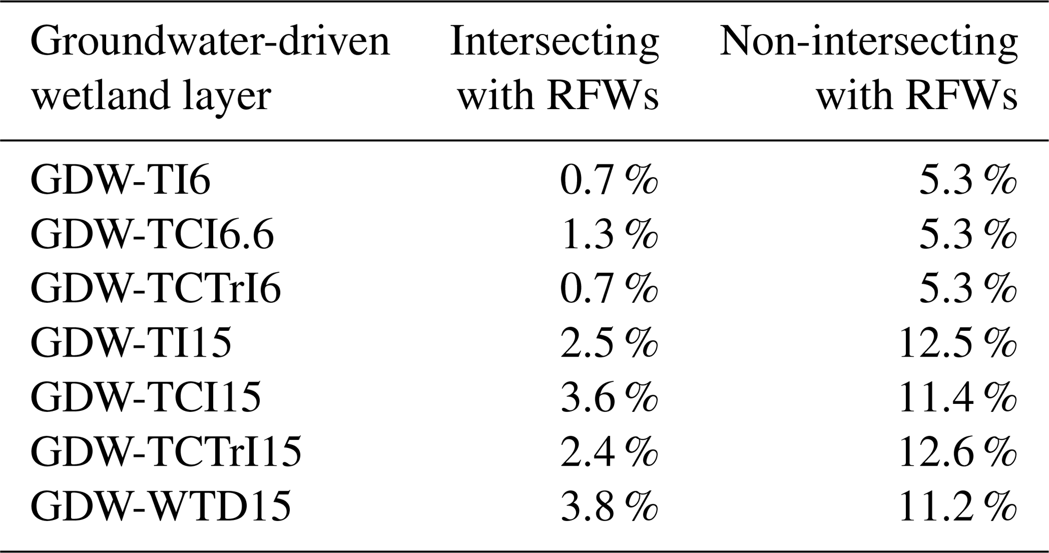
In line with many studies (Rodhe and Seibert, 1999; Curie et al., 2007; Hu et al., 2017), we define TI-based wetlands as the pixels with a TI above a certain threshold, defined to match a certain fraction of total land. In doing so, we prescribe the global GDW fraction as a chosen value, and the various TI formulations (Sect. 2.4.2) only change the geographic distribution of the corresponding wetlands. To apprehend the uncertainty related to the choice of the global GDW fraction, we tested two choices within the bounds derived from the global WTDs of Fan et al. (2013). In the first approach, we set the TI threshold such that the wet pixels (with high index values) cover 15 % of the land surface area, such as the fraction of WTD ≤ 20 cm according to Fan et al. (2013). The corresponding maps are noted as GDW-TI15, GDW-TCI15 and GDW-TCTrI15 in Table 2 and show fairly different patterns (Fig. 2b–d). The second approach assumes that the total wetland extent (this time including both GDWs and RFWs) covers 15 %. The TI thresholds are subsequently set such that the union of RFWs and GDW-TI (TCI/TCTrI), i.e., the composite wetlands, has the same extent as GDW-WTD. The resulting GDWs cover between 6 % and 6.6 % of the land area depending on the TI formulation and level of overlap with RFWs (Table 4) and are noted as GDW-TI6, GDW-TCI6.6 and GDW-TCTrI6. The patterns of these three maps are highly similar to those of GDW-TI15, GDW-TCI15 and GDW-TCTrI15, with diminished extents and densities (Fig. 2e–g).
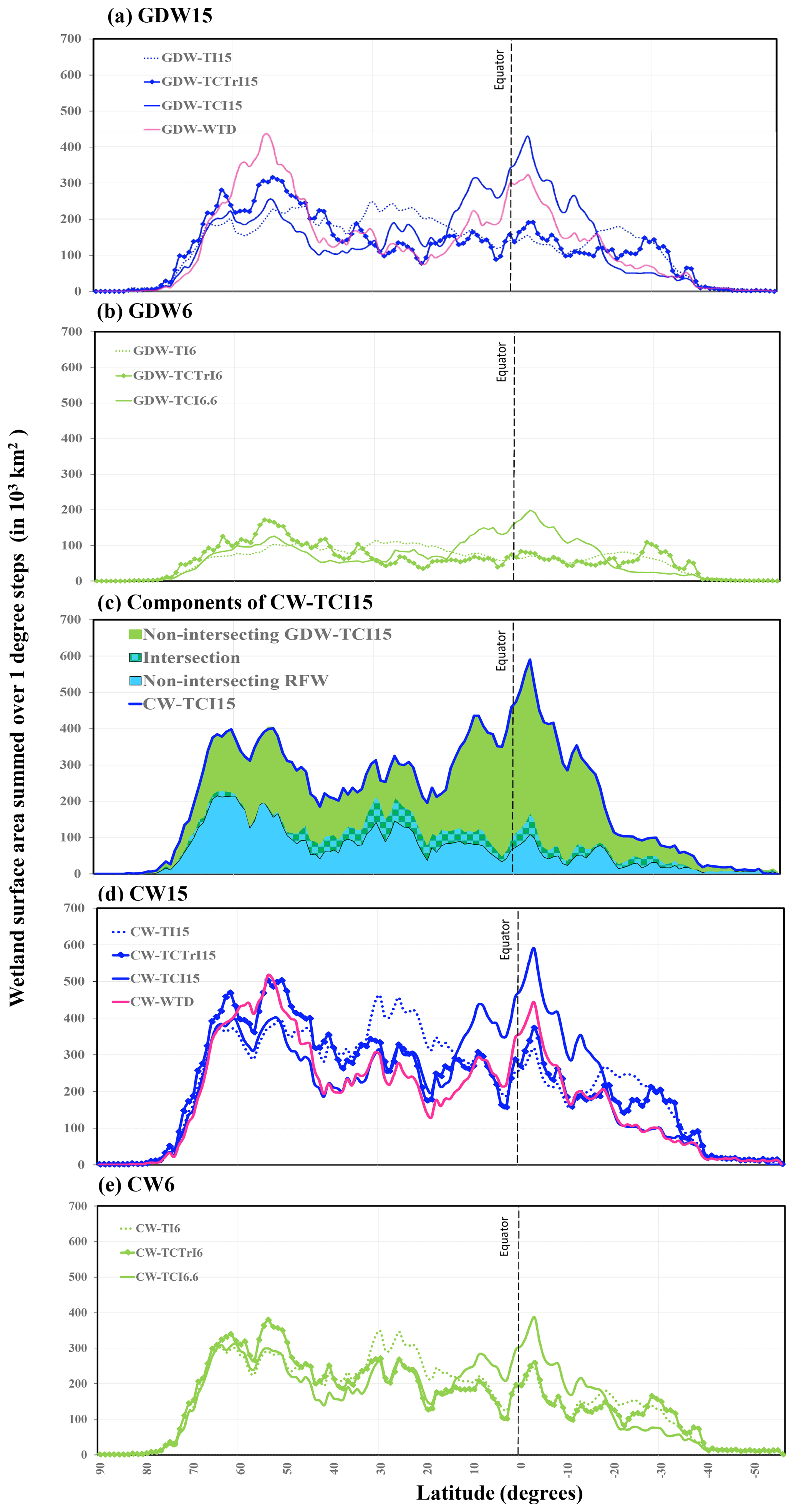
Figure 3Latitudinal distribution of different wetland maps: (a, b) GDWs, (c) components of CW-TCI15 and their intersection and (d, e) CWs. The wetland areas along the y axis are surface areas in each 1∘ latitudinal band.
3.3.3 Comparison of the proposed GDW maps
As shown in Table 2, seven GDW maps are developed, consisting of GDW-WTD (Sect. 3.2.1) and six GDW-TIs (Sect. 3.2.2). The GDW-WTD map contains high wetland extents over the northern latitudes (Fig. 2a), in contrast to the other six GDW maps. The diagnosed wetlands of GDW-TI maps (Fig. 2b, e) are equally distributed over well-known arid areas such as the Sahara and the Kalahari Desert, the Australian Shield and the Arabian Peninsula as in wet regions such as the West Siberian Plain and northern Canada (Fig. 2b, e). As a result, for a given threshold (15 % in Fig. 3a), the distribution of wetlands derived from the simple TI is nearly uniform over different latitudes. Lower thresholds on TI variants (Figs. 2e–g and 3b) obviously result in a smaller wetland extent, with no major change in the zonal pattern when the wet fraction threshold changes from 15 % to 6 % (Figs. 2b–d and 3a, b).
Introducing a climate factor in the form of effective precipitation in GDW-TCI6.6 and GDW-TCI15 increases the value of the wetness index in wet areas and decreases it in dry climates (Figs. 2c, f and 3a, b). Therefore, previously diagnosed wetlands with a TI in dry climates disappear and transfer to regions with wet climates (such as the Amazon basin and South Asia). However, because transmissivity values sharply change by several orders of magnitude over regions with small permeability, the patterns of GDW-TCTrI maps are nearly replicas of the low hydraulic conductivity distribution in GLHYMPS (e.g., large diagnosed wetlands in North America and central Asia; Fig. 2d, g). Although at times GDW-TCTrI coincides with famous wetlands such as the Pampas in South America (Fig. 2d, g and near 25∘ S in Fig. 3a), diagnosed wetlands extend far beyond the actual wet regions into neighboring arid or semi-arid zones; e.g., vast diagnosed wetlands in the western Siberian lowlands extend southward towards the Kazakh upland arid zones. In the absence of precise and consistent information on subsurface characteristics (particularly for cold areas), GDW-TCTrI shows low wetland densities in zones with the known effect of transmissivity, such as the Hudson Bay Lowlands and the Prairie Pothole Region.
Table 4Percent of overlap between GDWs and RFWs (percent of total land pixels).
3.4 Composite wetland (CW) maps
Each GDW map was overlapped with the RFW map to generate seven CW maps. Equi-resolution raster pixels of RFWs and GDWs were aligned to coincide exactly with each other. The resulting composite wetland maps are named with respect to their contributing GDW component (Table 2); e.g., the composite map containing RFW and GDW-TI6 is known as CW-TI6. These composite wetlands cover between 15 % and 22 % of the land surface area. Each CW map contains RFWs and GDWs and thus wetlands shared by both wetland classes (the intersection). The intersection between GDW and RFW maps is larger for TCI-based maps and GDW-WTD (almost one-third of RFWs intersect with these GDW maps) compared with TI- and TCTrI-derived GDW maps (Table 4). These intersection zones are further discussed in Sect. 4. The wetland extent in CWs is by definition larger than both RFWs and GDWs, and their spatial patterns depend on the contribution percentage of each component. As an example, in CW-TCI15, over most latitudes, the spatial pattern is similar to that of RFWs, except over the tropical zones where GDWs are far more extensive than RFWs, thus shaping the general latitudinal pattern (Fig. 3c). Changing the percentage of GDWs (between 6 % and 15 %) based on different TI formulations increases the wetland fraction of the CW maps to between 5.3 % and 12.5 % of the land area, but it does not considerably change their overall latitudinal pattern (Fig. 3d, e). In RFWs, large wetlands are present between 25 and 35∘ N (Fig. 3c), whereas in all GDW maps, the wetland extents over these latitudes are smaller than in other wetland regions (Fig. 3a, b).
4.1 Spatial similarity assessment
A difficulty inherent in the validation of any wetland map is the vast disagreements among available datasets and estimates. In this paper, we used independent validation datasets (explained in Sect. 2.5) that are not used in any step as input to our final products, but we made an exception for the GDW-WTD (derived from Fan et al., 2013), although it is a direct input to CW-WTD, and we used the total wetland fraction of GDW-WTD (corresponding to WTD ≤ 20 cm) to define the TI thresholds behind the TI-based CW maps. This exception is considered for two reasons. Firstly, we focus here on spatial patterns, which are completely independent between TI-based CW maps and GDW-WTD because of very different GW modeling assumptions and input data. Secondly, we also focus on wetlands rather than inundated areas, and on their detection under dense vegetation; GDW-WTD is one of the very few global datasets with these properties, but it results from a different method than Hu et al. (2017) and GLWD-3, so it can help to enrich the uncertainty discussion. All seven developed CW maps and the RFW map were evaluated using spatial coincidence, the Jaccard index (JI) and the spatial Pearson correlation (SPC) coefficient with respect to the validation datasets over the globe and in several regions, the latter of which are discussed in detail below.
Table 5Correlation between the developed and reference datasets (wetland fractions in 3 arcmin grid cells). The highest three values in each column are shown in bold format, and values used in Fig. 4 are highlighted in italic font.

The first evaluation criterion of spatial coincidence (SC) is defined as the fraction of pixels identified as wet in a validation dataset that are also detected in the composite wetland dataset:
SC is calculated at 15 arcsec resolution by intersecting CWs and validation datasets, and it ranges from 0 to 1, with higher values showing greater similarity between two datasets. For pair-wise comparisons of datasets with different wet fractions, the Jaccard index (JI) is better suited. This index is the fraction of shared wetlands in CW and the validation dataset over the size of their union:
JI ranges from 0 to 1 as well, and a zero index represents the case in which the two datasets are disjoint, and a value of 1 occurs if two datasets are exactly the same. The last criterion is the SPC. SPC is independent from the wet fractions in the CWs and evaluation datasets but is sensitive to the spatial distribution pattern in pair-wise comparisons. SPC values range from 0 to 1, with higher values showing greater similarity. Although the first two criteria were applied for comparison at the original 15 arcsec resolution, SPC was calculated based on aggregated wetland densities at 0.5∘ resolution.
Spatial similarity evaluations are displayed as radar charts in Fig. 4 for RFWs and the different CW maps for the globe and the selected regions. Because the values of the criteria are sometimes quite similar, three CW maps were selected for display in color for clarity, while the others are shown in grey (CW-TCI6.6, CW-TCI15 and CW-WTD).
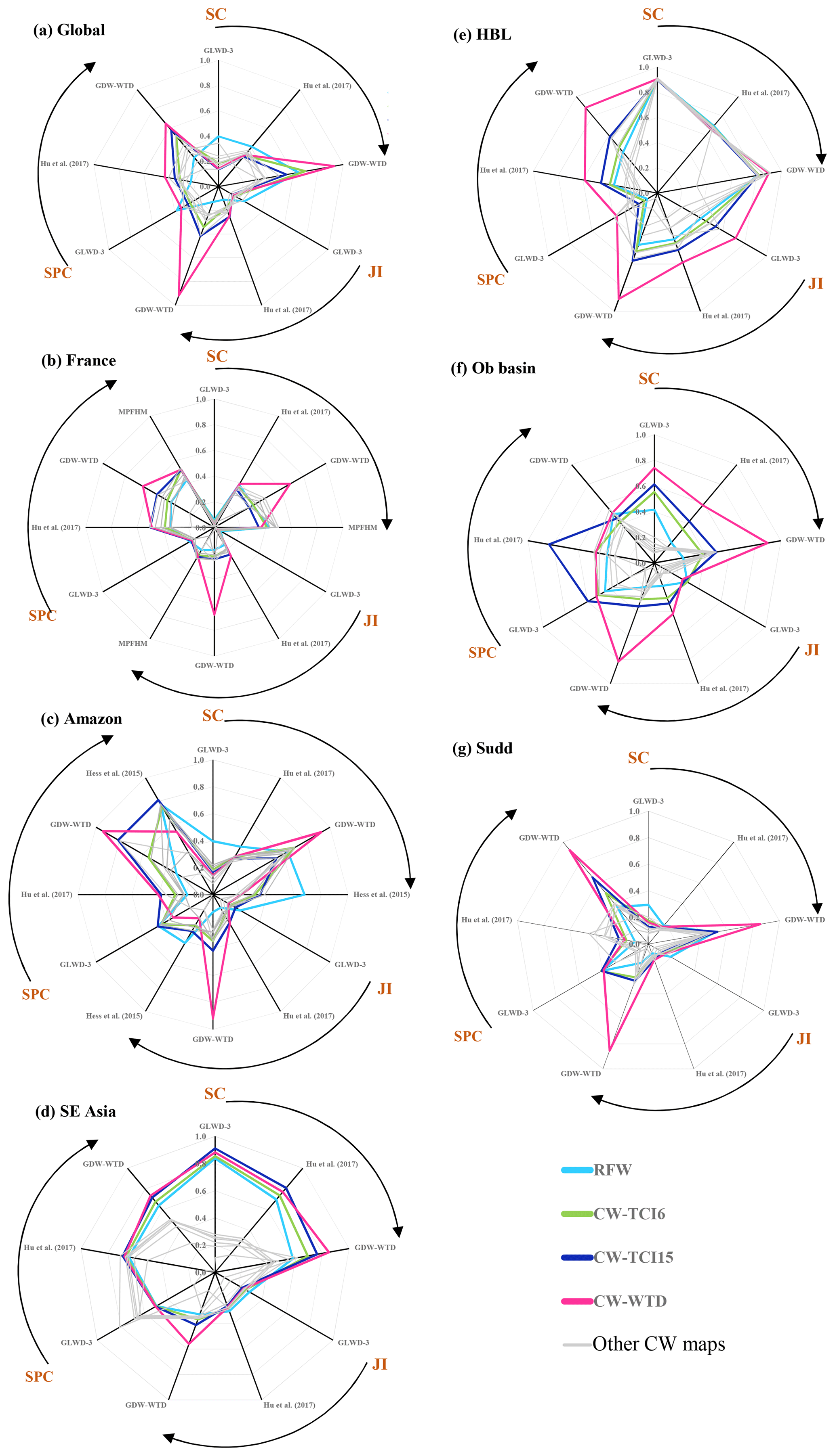
Figure 4Evaluation criteria between composite wetland maps and evaluation datasets for (a) the global scale, (b) France, (c) the Amazon, (d) Southeast (SE) Asia, (e) Hudson Bay Lowlands (HBL), (f) the Ob basin, (g) the Sudd swamp.
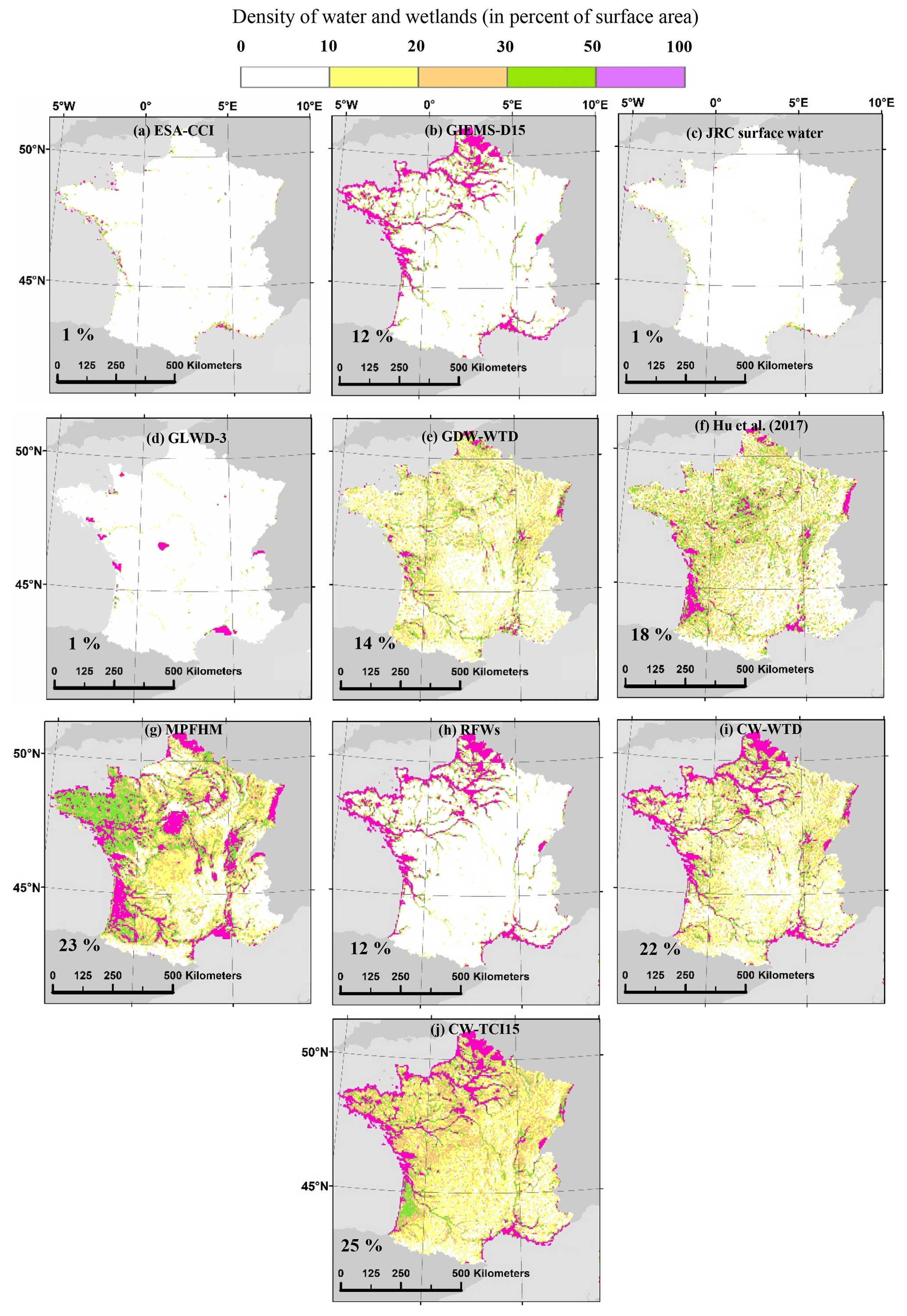
Figure 5Maps of wetlands in France according to different water and wetland datasets: (a–c) components of RFW, (d–g) validation datasets and (h–j) datasets generated in this study. The panels also give the mean areal wetland fraction of each dataset in the study area (using the mean fraction of each fractional wetland class of GLWD-3; cf. Sect. 2.5.1). The bounds of the study are the boundaries of metropolitan France.
4.1.1 Global analysis
With the exception of CW-WTD, which is always more similar to GDW-WTD because the latter is a component of the former, the validation criteria for the CW maps are rather small overall (between 0.2 and 0.6). However, the criteria are larger than the same values between the surface water and wetland datasets (less than 0.3 in Table 5 for the SPC of the globe and Table S1), showing their advantages. CW maps (especially CW-TCI maps) are more similar to GDW-WTD and Hu's map with respect to GLWD-3 because all but GLWD-3 share the GW modeling methodology. In contrast, the RFW map extends over a 60 % larger surface area than GLWD-3 and displays the highest similarity to GLWD-3, suggesting that wetlands in GLWD-3 are the regularly flooded ones. The inclusion of GDWs in the CW maps makes them depart from GLWD-3, but it markedly increases their similarity to the other two validation datasets for JI and SPC (e.g., SPC [RFW, GDW-WTD] = 0.3 versus SPC [CW-TCI15, GDW-WTD] = 0.6). As demonstrated in Fig. 4a (and also Table S1), increasing the GDW contribution from CW-TCI6.6 to CW-TCI15, as an example, also improves the similarity criteria (except the SC for GLWD-3 and GDW-WTD), justifying the need to account for the GDWs to provide a comprehensive description of wetlands. This is clearer for the global spatial correlation values which all increase when the contribution of GDW is increased from 6.6 % to 15 % (Table S1, first row block).
The following section breaks down the comparative wetland representation between our maps and that of the validation datasets at the regional scale. The selected regions encompass different climates, vegetation covers and ecosystems, both within and outside important wetland areas of the world, to assure the applicability of CW maps. These six regions are France in the temperate climate, the Amazon basin and Southeast Asia over the tropical zone, the cold boreal areas of the Hudson Bay Lowlands and the Ob River basin and the Sudd swamp in South Sudan with a semi-arid savannah climate.
4.1.2 France
Over France, wetland fractions from the validation datasets are highly inconsistent (Fig. 5). Visible range satellite imagery (JRC surface water) shows the smallest wet fraction (1 %). The GLWD-3 and ESA-CCI maps also produce low wetland coverage, whereas GIEMS-D15, which essentially forms the RFW map, gives 12 % coverage concentrated along the coastline and over the floodplains of the northern rivers. Wetlands from GW modeling-based datasets cover even larger areas (14 % and 18 % in GDW-WTD and Hu et al., 2017) and are scattered countrywide, except for the French Pyrenees and the Alps, with moderately denser wetlands along large rivers (such as the Rhine floodplain at the eastern border) and the Landes (southwestern shore). The MPHFM map (Berthier et al., 2014) can be considered as the most comprehensive validation dataset for the country because it relies on hydromorphic soil properties and was extensively validated. This map shows much larger wetland extents (23 % of France) than the above estimates because of its inclusion of both floodplains (along the Loire, Saône and Rhône rivers) and groundwater-driven wetlands, including those over the weakly permeable granites of Brittany (shown in green in Fig. 5g). These notorious wetlands are not considered in the global validation datasets but are captured to a good extent in CW maps (Fig. 5i, j).
By combining RFWs (which overlap with 20 % of MPHFM) and GDWs, our CW maps capture many features of the MPHFM map, including the total wetland extent (23 % for MPHFM versus 22 % and 25 % for CW-WTD and CW-TCI15) and correctly capturing most of the coastal and riparian wetlands (Fig. 5). The larger wetland fraction in MPHFM and CW maps is consistent with the work of Pison et al. (2018), who found that (wetland-driven) methane emissions over France deduced from atmospheric inversion were almost a third higher than direct estimates, from anthropogenic inventories and biogeochemical models driven by global wetland datasets (e.g., the overlap of GLWD and SWAMPS in Saunois et al., 2016). The added value of CW maps is demonstrated by the higher similarity criteria between CW maps such as CW-TCI15 and MPHFM (SPC = 0.52) than between surface water maps such as GIEMS-D15 and MPHFM (SPC = 0.43). However, it is difficult to identify the best CW map over France based on the similarity criteria against MPHFM because four of our CW maps (all shown in grey in Fig. 4b) display nearly the same values (Table S2).
4.1.3 Amazon basin
The Amazon River basin is considered one of the richest tropical wetland ecosystems in the world (Mitsch and Gosselink, 2000). For ease of comparison, we limited our study to the domain of Hess et al. (2015), which covers 5 million km2 (Fig. 6). RFWs (mostly consisting of GIEMS-D15) show a pattern rather similar to that of GLWD-3 and Hess et al. (2015) (Figs. 4c and 6d, g, h), covering only the main drainage network of the Amazon and certain seasonally flooded wetlands and floodplains. However, certain spatial disagreements exist among these three datasets in seasonally flooded wetlands such as Llanos de Moxos (12∘30′–17∘30′ S, 63–68∘ W), the Roraima savannah and the Negro River basin (2∘ N–2∘ S, 60–65∘ W), which are larger in RFWs and Hess et al. (2015) than in GLWD-3.
The CW maps capture the wetland pattern of GDW-WTD and Hu et al. (2017) considerably better than RFWs (Fig. 6), highlighting the significance of groundwater wetlands over the Amazon. Wetland densities in CW maps, Hu et al. (2017) and GDW-WTD are more realistically high over the leached and swampy soils of the northern Amazon basin (e.g., Japurá–Solimões–Negro moist forests) and over the Purus–Madeira ecoregion, in line with recent estimates of wetlands and peatlands (Hess et al., 2015). This result suggests that the extended shallow peatlands of South America are the main causal contributor to the global tropical wetland extent (Gumbricht et al., 2017). The higher wetland densities of CW maps with respect to all satellite observations over these particular areas can be attributed to the coincidence of GDWs and dense rainforests (covering almost two-thirds of this domain), with large non-flooded wetlands over the Amazon. River channels and surrounding floodplains are better represented in CW maps, as compared with Hess et al. (2015), due to the inclusion of the RFW component. Similarly, CW compares well to other datasets because almost none of the river floodplains are delineated in Hu et al. (2017), and GDW-WTD misses the Tapajós River floodplain and portions of the downstream Amazon corridor. However, CW maps represent the wetland extent in lower density over grassland/savannahs and the Andes dry regions compared with the validation datasets.
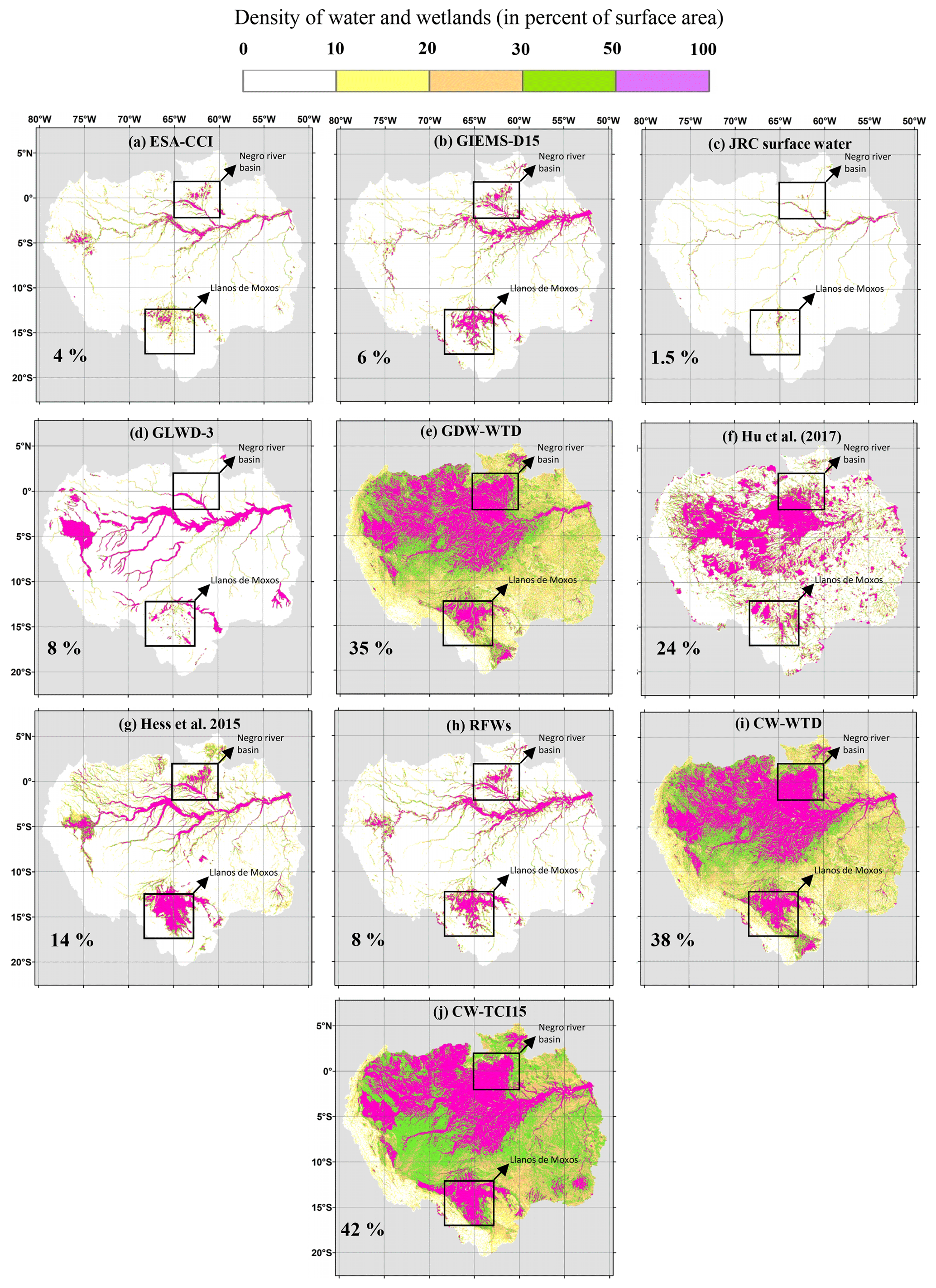
Figure 6Maps of the Amazon River basin wetlands according to different water and wetland datasets: (a–c) components of RFW, (d–g) evaluation datasets and (h–j) datasets generated in this study. The panels also give the mean areal wetland fraction of each dataset in the study area (using the mean fraction of each fractional wetland class of GLWD-3; cf. Sect. 2.5.1). The bounds of the basin are taken from Hess et al. (2015).
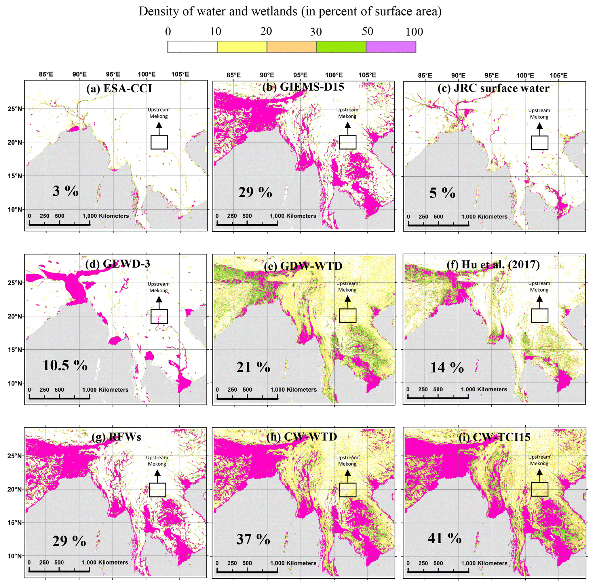
Figure 7Maps of the Southeast Asian wetlands according to different water and wetland datasets: (a–c) components of RFW, (d–f) evaluation datasets and (g–i) datasets generated in this study. The panels also give the mean areal wetland fraction of each dataset in the study area (using the mean fraction of each fractional wetland class of GLWD-3; cf. Sect. 2.5.1). The bounds of the study window are 5–28∘ N, 82∘30′–108∘ E.
4.1.4 Southeast Asian deltas
The selected window over South and Southeast Asia stretches over notably wet regions, similar to the Amazon, but with severe human interference and deforestation (Miettinen et al., 2011; Stibig et al., 2013). In Southeast Asia, RFWs (mostly composed of GIEMS-D15) are larger than all validation datasets (Fig. 7d–g) because GIEMS-D15 also detects inundated areas associated with cultivation activities such as rice paddies (Fluet-Chouinard et al., 2015), which are not considered in inventories and GW modeling-based estimates. Over the window, RFWs and CWs coincide with the majority of wetlands in the validation sets, particularly over the Ganges–Brahmaputra floodplain, northern Indochina and Yunnan Plateau subtropical forests (Fig. 4d; SC between 0.59 and 0.91), showing the good agreement of our developed maps with respect to spatial patterns. As a general rule in Southeast Asia, floodplains and deltas (Ganges, Brahmaputra, Irrawaddy, Mekong and Red rivers) extend over larger areas in CW maps than in validation maps (Fig. 7), giving a more realistic extent than those in Fan et al. (2013) and Hu et al. (2017), considering the vast flood irrigated cultivation lands along floodplains. However, only a few small wetlands in the validation datasets are missed in RFWs (and CW maps), such as the upstream Mekong River corridor (near 20∘ N–102∘ E) and Irrawaddy River (near 25∘ N–97∘ E) in GLWD-3.
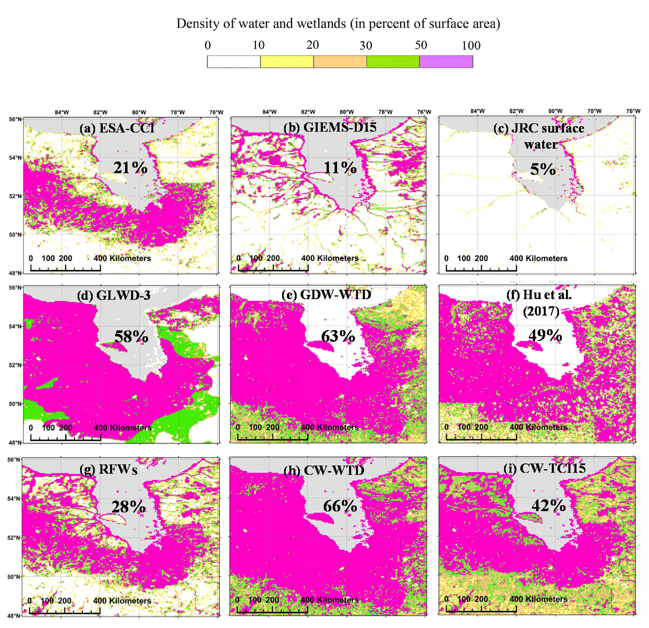
Figure 8Maps of the Hudson Bay Lowlands wetlands according to different water and wetland datasets: (a–c) components of RFW, (d–f) evaluation datasets and (g–i) datasets generated in this study. The panels also give the mean areal wetland fraction of each dataset in the study area (using the mean fraction of each fractional wetland class of GLWD-3; cf. Sect. 2.5.1). The bounds of the study area are 48–56∘ N, 76–86∘ W.
The CW-WTD and CW-TCI15 maps present patterns that are highly similar to each other (Fig. 7h, i) and to the validation datasets. However, high similarity criteria (especially SC) can be the result of the large extension of RFWs, itself overlapping almost all of the wetlands in the validation datasets. In addition, the similarity of CW-WTD and CW-TCI15, also derived from similarities between their GDW components, notes that groundwater wetland formation is almost completely explained by topography and climate (of the TCI formulation) in these areas and the negligible role of subsurface characteristics included in GDW-WTD.
4.1.5 Hudson Bay Lowlands
The Hudson Bay Lowlands (HBL) are a vast flat wetland area in the low subarctic regions of North America dominated by extensive peatlands, swamps and marshes (Mitsch and Gosselink, 2000; Packalen et al., 2014), where below-freezing temperatures for most of the year reduce drainage in the soil layer (Hamilton et al., 1994). A systematic contrast is noted between inundation maps (Fig. 8a–c; maximum wet fraction: 21 %) and validation datasets (Fig. 8d–f; minimum wet fraction: 49 %), underlining the inability of satellite imagery to capture wetlands in this area (e.g., Landsat images used in JRC surface water; Fig. 8c). Surprisingly, GLWD-3 has a pattern notably similar to that of the other two validation maps due to the comprehensive wetland maps in Canada available to its developers. Moreover, HBL is one of the few regions where similarity indices sharply increase with increased GDW contribution (Table S1). The Jaccard index rises from 0.46 to 0.53 when increasing the total GDW extent from 6.6 % to 15 % between CW-TCI6.6 and CW-TCI15. CW maps perform fairly well, particularly CW-WTD, which predominantly obtains the highest validation criteria (Fig. 4e). Due to an explicit parameterization of the permafrost (adjusted to reproduce the “observed wetland areas” in North America; Fan and Miguez-Macho, 2011), dense wetlands are extended south of 50∘N in the GW model by Fan et al. (2013), which are less dense in CW-TCI15 in the absence of a soil-freezing mechanism. Comparing wetlands detected through satellite imagery and validation datasets, GW modeling appears to be the best wetland delineation method over boreal zones due to nonpermanent surface inundation, shallow WTD or snow/ice cover.
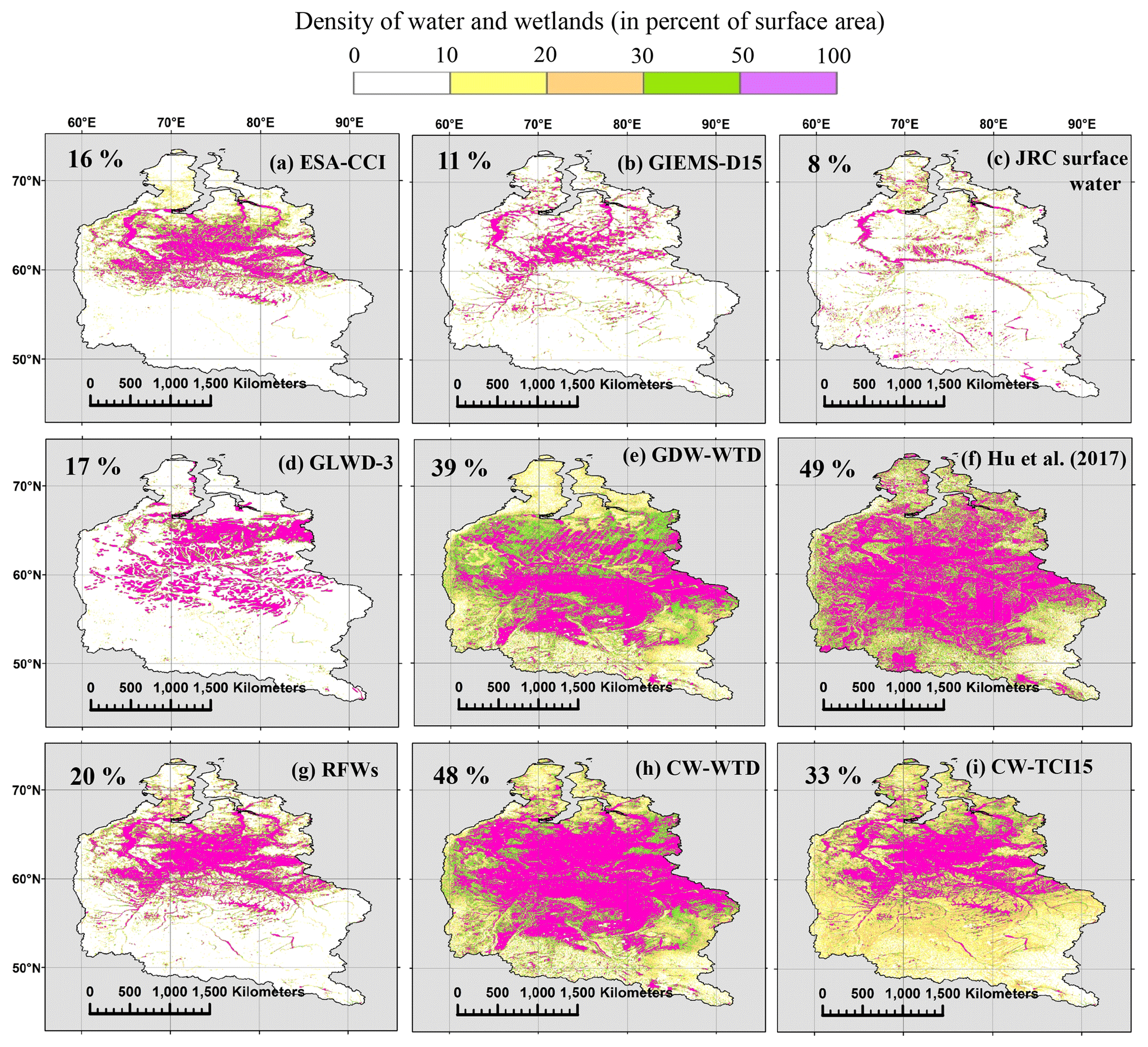
Figure 9Maps of the Ob River basin wetlands according to different water and wetland datasets: (a–c) components of RFW, (d–f) evaluation datasets and (g–i) datasets generated in this study. The panels also give the mean areal wetland fraction of each dataset in the study area (using the mean fraction of each fractional wetland class of GLWD-3; cf. Sect. 2.5.1). The bounds of the basin are taken from the HydroBASINS layer of HydroSHEDS.
4.1.6 Ob River basin
The Ob River basin in western Siberia extends over km2. The annual variability of the inundated area is large (e.g., Mialon et al., 2005), making this basin one of the largest wetland complexes in the world, which contributes to buffer peak discharge during the flooding period (Grippa et al., 2005). Wetland fractions in different datasets compare similarly to HBL, except for GLWD-3, which appears to underestimate the total wetland extent although the climatic and geomorphologic properties are nearly alike. Datasets recognizing the contribution of GW to wetland formation (Fig. 9e, f, h, i) indicate consistently higher wet fractions than others. However, CW-TCI15 appears to miss wetlands south of 60∘ N that are extended to the upstream Ob River basin near 50∘ N in both GDW-WTD and Hu et al. (2017), most likely due to the permafrost effect on wetland formation. With respect to the evaluation criteria, CW-WTD often displays better performances, although CW-TCI15 shows the highest SPC. We also find that CW-TCI15 outperforms CW-TCI6.6 for all criteria and validation dataset combinations (Table S1). TCTrI-based CW maps fail to surpass others in the validation process, considering that we used the transmissivity map without the permafrost adjustment due to its imprecise representation of hydraulic conductivity in these zones (Sect. 2.4.4). CW-WTD tends to better capture the wetland extent and spatial pattern, with more concentrated wetlands in the downstream lowlands and northwestern regions (65∘ N–65∘ E) of the basin due to RFWs. Overall, considering the wetland fraction solely attributed to GDWs in CW-TCI15 and CW-WTD (13 % and 29 % of the basin area) and the difference found between the inundation and validation dataset (Fig. 9, first and second row), it becomes clear that the uncertainty of the wetland extent and spatial pattern is rather high over boreal zones.
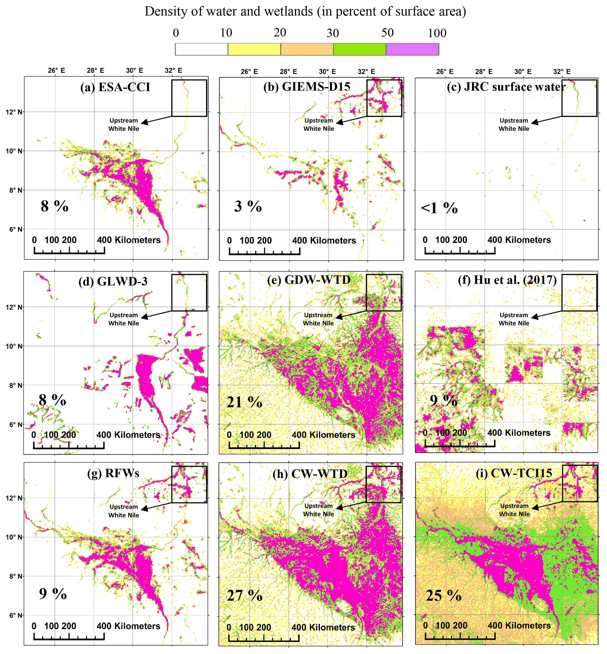
Figure 10Maps of the Sudd swamp wetlands according to different water and wetland datasets: (a–c) components of RFW, (d–f) evaluation datasets and (g–i) datasets generated in this study. The panels also give the mean areal wetland fraction of each dataset in the study area (using the mean fraction of each fractional wetland class of GLWD-3; cf. Sect. 2.5.1). The bounds of the study area are 4∘30′–14∘ N, 24∘30′–34∘ E.
4.1.7 Sudd swamp
This large wetland is located in eastern South Sudan, nearly 300 m above mean sea level, and is the largest freshwater wetland in the Nile basin (Sutcliffe et al., 2016). The Sudd swamp extent estimations are highly uncertain in the literature, ranging from 7.2 to 48×103 km2 (Mohamed et al., 2004, and references therein). Over the selected window, the wetlands and surface water distribution is also highly disparate and varies from 1 % to 27 % for different datasets (Fig. 10). Additionally, wetlands in Hu et al. (2017) are rather patchy and show sharp density changes with what seems to be periods of 0.5∘. Because GLWD-3 appears to represent only flooded wetlands (with the same wetland fraction of RFWs and overlapping with one-third of them), and the study of Hu et al. (2017) contains technical issues, GDW-WTD can be considered as the only comprehensive validation dataset over the Sudd swamp.
The CW datasets in Fig. 10 show high wetland densities in the central floodplain, in rather good agreement with GLWD-3, GDW-WTD and regional estimates of saturated soil (compared with visuals in Mohamed et al., 2004, and Mohamed and Savenije, 2014). CW-WTD compares more similarly to validation datasets, closely followed by CW-TCI15 (Fig. 4g), but the main difference between these two CW maps is that the groundwater wetlands in CW-TCI15 are extended southwest into the southern national park (over local flat valley bottoms) but are more concentrated over the main floodplain in the SE–NW direction for CW-WTD. The total wetland fraction is nearly equal in CW-TCI15 and CW-WTD (25 % and 27 % of the selected window area), underlining a primary role of topography and climate in wetland formation. Considering the wetland fraction in the RFW map (mostly consisting of ESA-CCI wetlands) and GDW-WTD, groundwater wetlands appear to be the dominant feature in the Sudd swamp, as is the case for CW-WTD and CW-TCI15. The added value of CW maps with respect to GDW-WTD is not substantial, but they additionally contain the seasonally flooded plains downstream of the White Nile (top right of the selected window in Fig. 10g, 12–14∘ N, 32–34∘ E), which are not completely captured by validation datasets due to the inclusion of RFWs.
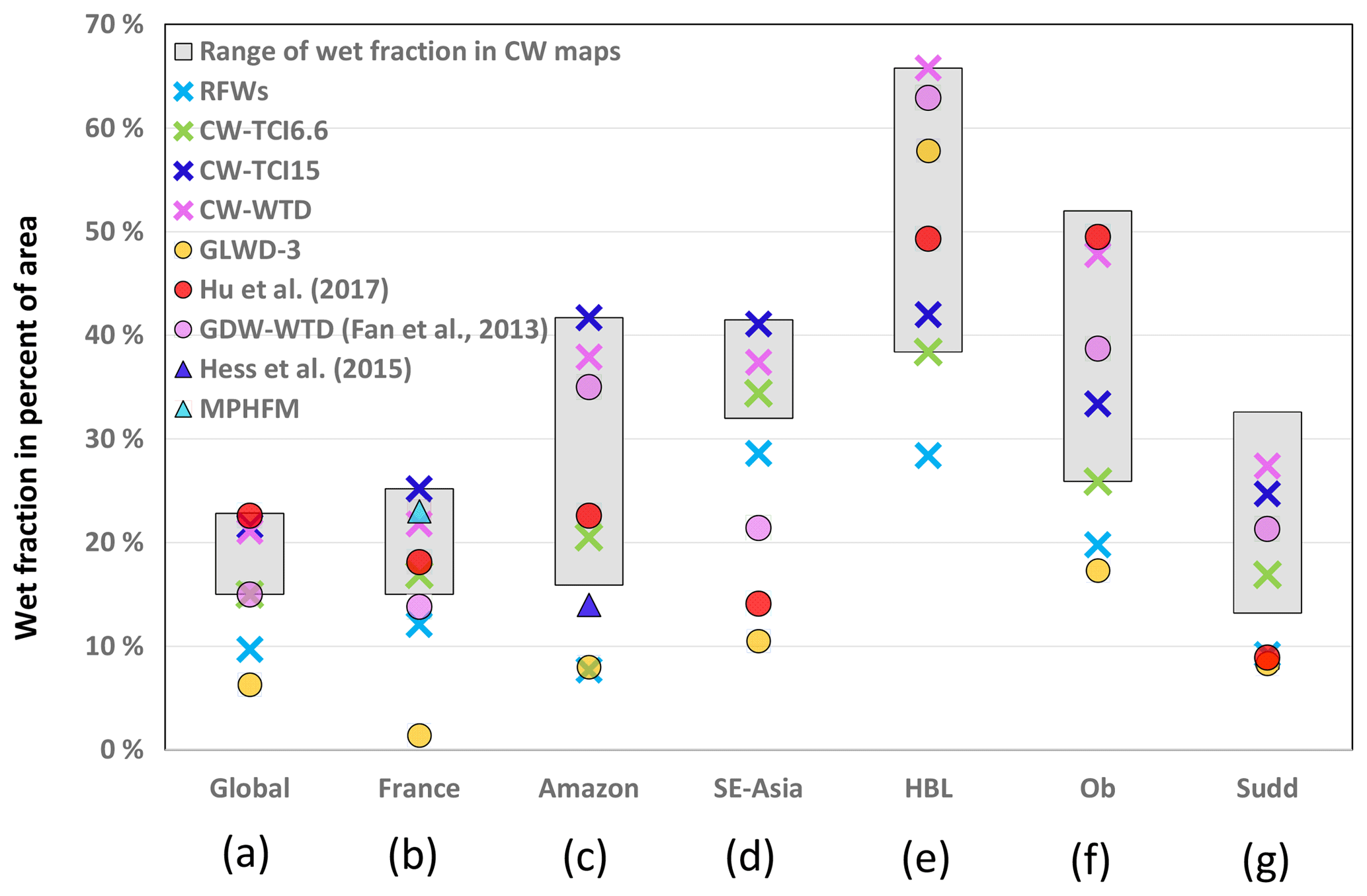
Figure 11Total wet fractions for RFWs, different CW and validation datasets, at the global scale and in the studied regions (values in percent of the corresponding land surface area). Only three CW maps are shown in color, and others are displayed in the grey range.
4.2 Wetland extents
Figure 11 shows that the global wetland fractions of the different CW maps are in range of those in Fan et al. (2013) and Hu et al. (2017), with twice the wetlands in GLWD-3, itself 60 % smaller than the RFW extent. Over France (Fig. 11b), the wetland fraction of the CW maps is notably similar to that of MPHFM, which is a calibrated and validated wetland dataset that includes the GDWs. The regional uncertainty of CW maps is smaller over subtropical areas and higher over boreal and tropical zones. For instance, although the global wetland extents of CW-WTD and CW-TCI15 are nearly equal, the former contains 52 % more wetlands over the Hudson Bay Lowlands. However, in Southeast Asia, where RFWs have a rather large contribution to total wetlands, CW maps are in relative agreement on wetland extents, whereas the validation dataset appears to critically underestimate the wetland extents. The underestimation of global validation datasets, especially GLWD-3, is quite clear in France, the Amazon and the Ob River basin. Nevertheless, regional differences in wetland fractions among CW maps reaching up to 25 % in the HBL and the Amazon basin (due to the effect of permafrost in northern latitudes and high effective precipitation over the tropics) make our estimates uncertain as well. Additionally, the uncertainty of the reference validation datasets is almost always higher than that of CW maps (global: CW 7 %, validation 17 %; Ob basin: CW 25 %, validation 32 %).
5.1 Uncertainties of the CW maps and underlying layers
It must be stressed that the uncertainty of the proposed CW maps is high, owing to several factors impeding the accuracy of the RFW and GDW maps. The uncertainty of the RFW map comes from the three input layers (ESA land cover, GIEMS-D15 and JRC surface water) and the lack of accuracy of the remote sensing products they rely on (shown by their large range of global flooded extents, from 1.5 % to 7.7 % excluding lakes). Of particular relevance is the uncertainty of GIEMS-D15, which contributes a lot to the high fraction of RFWs, and exhibits a small overlap with the other two datasets (less than 10 % of inundated areas in GIEMS-D15 are confirmed by either ESA land cover or JRC surface water). Taking GLWD as a reference, Adam et al. (2010) concluded that inundation extents are overestimated in GIEMS (0.25∘ product of Papa et al., 2010) over parts of northern Europe and India “because very wet soils may be wrongly identified as inundated”, but this kind of error is not a major issue to identify wetlands, instead of inundated areas, as targeted by the CW maps. In India and Southeast Asia, GIEMS-D15 also includes areas with flooded irrigation, including large rice paddies, which correspond to artificial wetlands, not recognized in GLWD. Eventually, it is plausible that the RFW contribution from GIEMS-D15 is overestimated, but it must also be underlined that GLWD is not an exhaustive reference as it likely lacks some wetlands, as reported by Adam et al. (2010) and in Sect. 4.2.
Regarding the GDW maps, two major sources of uncertainty can be identified, related to modeling and thresholding. Whatever the GW modeling involved (simplified based on wetness indices, or direct like in Fan et al., 2013), a major challenge is to define thresholds on TI or WTD to separate the wet and non-wet pixels. Following the existing literature, we defined wetlands as areas where the mean WTD is less than 20 cm, and this WTD threshold was translated into the TI threshold defining the same global wetland extent (15 %). Any error on this extent because of modeling errors will propagate to TI-based wetland mapping. In particular, the steady-state assumption and 1 km resolution used by Fan et al. (2013), as well as their imperfect input data, only lead to a “first-order estimate of global land area likely affected by shallow groundwater”, according to the authors. Nevertheless, the threshold choices remain subjective in the absence of a consensual global wetland map and definition, and the related uncertainty in wetland extent was shown to amount to a few percent of the total land area based on sensitivity analyses for reasonable values of the different thresholds (Sect. S2, Figs. S3 and S4).
We also considered several classic variants of the TI to conclude that the TCI (topography–climate wetness index), also favored by Hu et al. (2017) with a modified formula, offers the best correspondence with the validation datasets. The original TI did not capture the wetland density contrasts between arid and wet areas, and the inclusion of subsurface transmissivity in TCTrI induced overly sharp density contrasts that did not always match the recognized patterns of large wetlands. This does not question the role of transmissivity in forming wetlands, but calls for improved global transmissivity datasets or new methods to supply a more continuous description of transmissivity than those currently proposed based on discrete classes of lithology (Hartmann and Moosdorf, 2012; Gleeson et al., 2014) or soil texture (Fan et al., 2013). Particular attention also needs to be given to the effect of permafrost on wetland formation, but simple maps are probably not sufficient to describe the complexity of hydrology–permafrost feedbacks, especially under global warming (Walvoord and Kurylyk, 2016).
The resolution of the input datasets is also prone to errors if coarser than the target wetlands. It is the case for transmissivity, as discussed above, and for climate input, at the 0.5∘ resolution for both GDW-TCI and GDW-WTD, which may lead to anomalous discontinuities, although they are not discernible in Fig. 2a, c, f. More relevant is the resolution of topography, at 15 and 30 arcsec for the TI calculation (Marthews et al., 2015) and WTD modeling (Fan et al., 2013), respectively. An important consequence is that the pixels of our 15 arcsec wetland maps are either fully wet or fully non-wet, which is obviously wrong in many places with patchy wetlands in small depressions or along headwater streams. A finer delineation can be expected from higher-resolution DEMs, such as HydroSHEDS or the MERIT (Multi-Error-Removed Improved-Terrain) DEM of Yamazaki et al. (2017), both offering a worldwide 3 arcsec resolution.
Finally, it must be underlined that the RFW, GDW and CW maps largely overlook the loss of wetlands induced by anthropogenic pressures, estimated to affect 30 % to 50 % of undisturbed or potential wetlands (Finlayson et al., 1999; Sterling and Ducharne, 2008; Hu et al., 2017), mostly due to urbanization and agricultural drainage. This feature is especially true for GDWs because most human influences were neglected in the input datasets (climate, topography, transmissivity and sea level) for global WTD modeling. In contrast, the RFW map was derived by overlapping satellite imagery for the contemporary period (past 5 to 34 years), thus showing most human-induced changes on the surface water, including artificial wetlands linked to flooded irrigation (Adam et al., 2010) or the way in which damming shifts wetlands to lakes or drylands (Pekel et al., 2016). Nevertheless, the overlap of several inundation datasets with different historical depths was intended to minimize these disturbances, as justified by the higher spatial correlation between the inundation datasets and the CW maps than between themselves. Therefore, by construction, the proposed CW largely corresponds to potential wetland. Considering that the loss of natural wetlands exceeds the extent of artificial ones by far, they have a larger extent than actual wetlands, making validation all the more complicated.
5.2 Selection of two representative CW maps
If none of the resulting CW maps systematically over-perform the others, two of them usually display the best similarity scores, namely, CW-TCI15 and CW-WTD (Fig. 4, Tables 5 and S1–S7). These two datasets (hereafter simply referred to as “CW maps”) have many similarities, and by construction, they have almost the same wetland extent (ca. 21 %), and the combination with RFWs reduces the differences found between the corresponding GDWs in boreal and tropical areas (Fig. 3). Both CW maps are among the highest estimates of global wetland, considerably larger than GLWD-3 and close to Hu et al. (2017). An interesting point is that the SPC between these two CW maps and the existing wetland datasets is higher than the SPC among these existing datasets (Table 5), which is rather low (e.g., the SPC between JRC surface water and GIEMS-D15 is 0.4). This observation underscores that the two outperforming CW maps reconcile the differences between existing wetland maps, whether they focus on RFWs (ESA-CCI, GIEMS-D15 and JRC surface water) or also encompass non-inundated wetlands (GLWD-3, GDW-WTD and Hu et al., 2017).
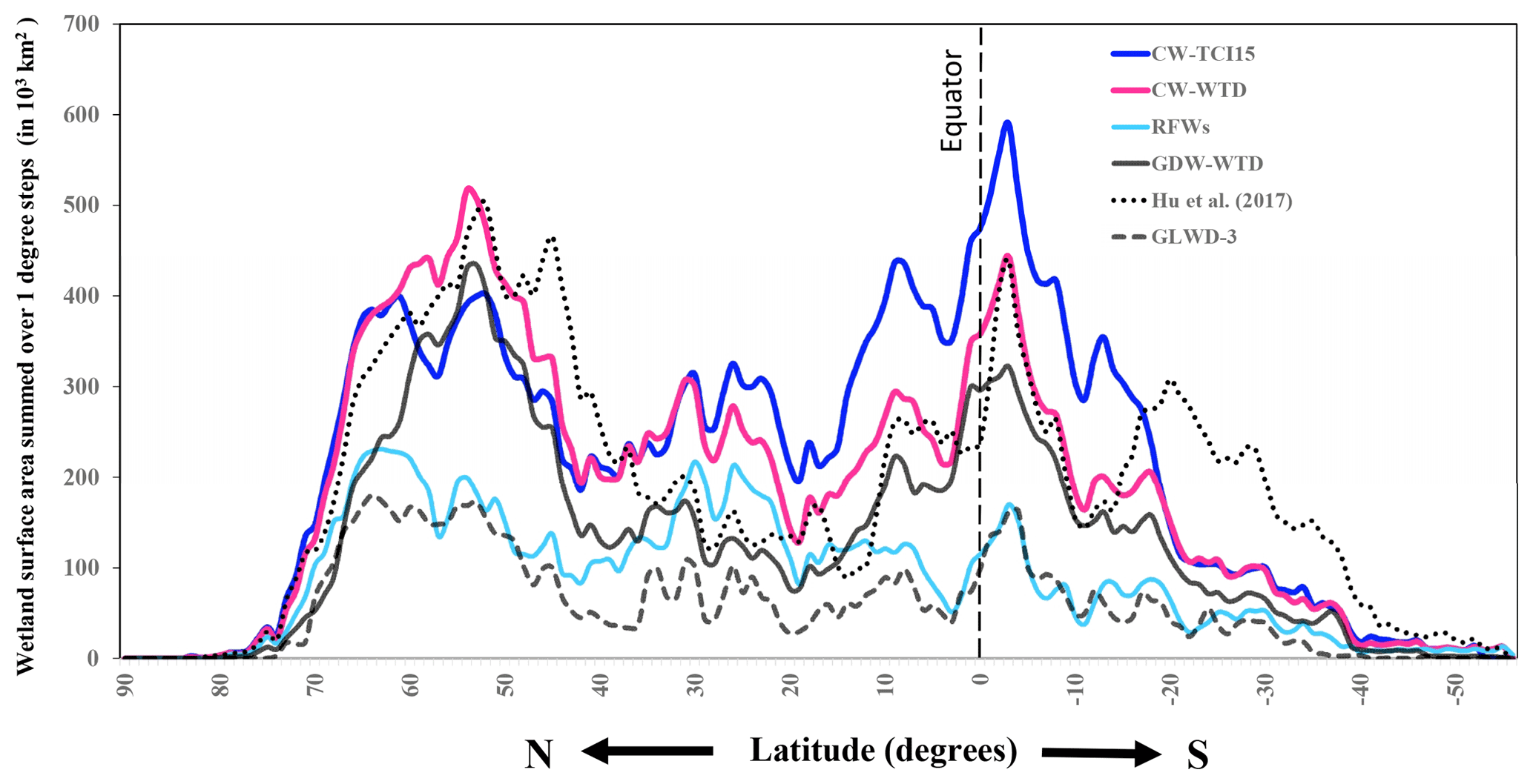
Figure 12Latitudinal distribution of the selected CWs and evaluation datasets. The wetland areas along the y axis are surface areas in each 1∘ latitudinal band.
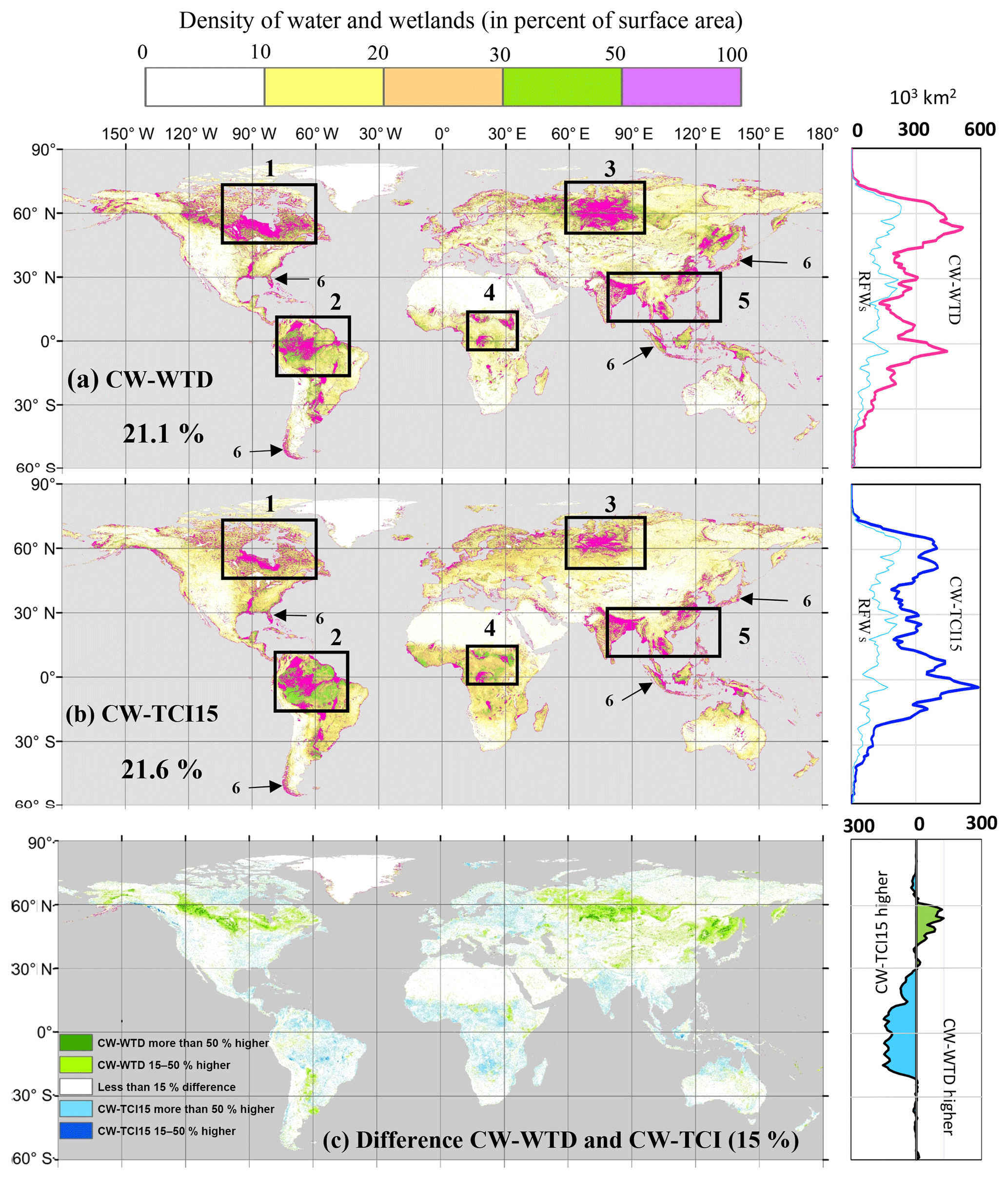
Figure 13Wetland density (as percent area in 3 arcmin grid cells) (a) in CW-WTD, (b) in CW-TCI15 and (c) the difference between them. Numbers in (a) and (b) refer to the wetland hotspot windows explained in Sect. 5. For zonal wetland area distributions (right-hand charts), the area covered by wetlands in each 1∘ latitude band is displayed.
5.3 Zonal patterns
Despite many similarities, the zonal distributions of the CW maps, RFWs and validation datasets are sometimes different. Generally, wetland datasets such as GLWD-3 and GDW-WTD appear to underestimate global wetland extents with respect to CW maps (Fig. 12 and the visuals for France and Southeast Asia, Figs. 5 and 7). The latitudinal patterns are also different among maps in Fig. 12, particularly over the tropics and the boreal zones. Although the wetlands in all validation datasets and CW-WTD are densely concentrated between 50 and 60∘ N, in the RFW map, the northern subtropical (25–35∘ N) and boreal (60–70∘ N) wetlands are of a similar extent (1.9 and 2.0 million km2), and in CW-TCI (15 %), tropical wetlands (10∘ N–10∘ S) globally outweigh others (covering almost 9 million km2). In fact, tropical wetlands in both CW maps are much more extensive than the maximum reported wetland extents for these latitudes in the literature (almost 5.6 million km2 in Hu et al., 2017). This result is in accordance with recent studies signalling an underestimation of tropical wetlands and the subsequent underestimation of their effect on energy, water and carbon cycles (Collins et al., 2011; Gumbricht et al., 2017; Wania et al., 2013).
Focusing on the differences between CW maps, because the two selected maps are constrained to share the same GDW extent, a trade-off exists between northern and tropical wetlands. In CW-WTD, northern wetlands extend further south into the Sakhalin taiga and Prairie Pothole Region, as shown by the green belt between 40 and 60∘ N in Fig. 13c. This southward extension is actually stronger than the permafrost zones (Gruber, 2012), suggesting that the description of the permafrost region in CW-WTD leads to wetland densities that are too strong. However, in the absence of an explicit mechanism for freezing and permafrost in the TCI formulation, CW-TCI15 is prone to underestimating boreal wetlands. Additionally, the difference between the CW maps over the humid tropical zones is consistent with the fact that TCI assumes that effective precipitation is entirely available for wetland formation, while it also contributes to surface runoff in the model used by Fan et al. (2013).
5.4 Relative role of RFWs and GDWs
Based on the intersection areas between RFWs and GDWs (Table 3) and the global CW fractions, 55 % of the global composite wetlands are solely groundwater-driven, with varying contribution levels in different ecoregions and climate zones. GDWs are the main wetland classes in the tropics and to a lesser extent in the boreal zones. RFWs dominate over the North American lowlands (Fig. 8), Southeast Asia (Fig. 7) and coastal areas and the tropical and subtropical transitional latitudes (Figs. 3c and 12).
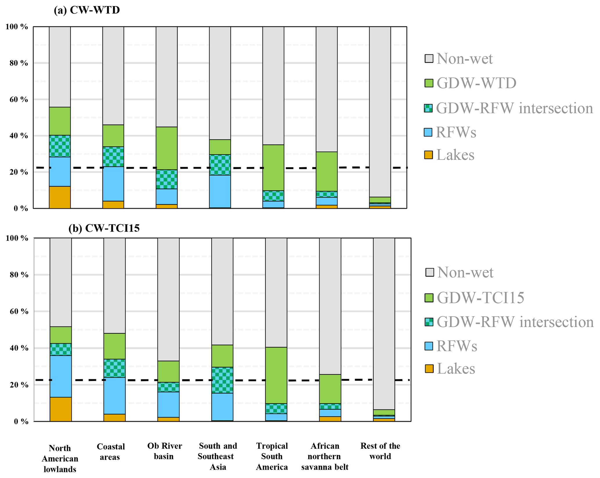
Figure 14Contribution of non-wet areas, lakes, RFWs, GDWs and their intersection in the wetland hotspot window shown in Fig. 13 (a) in CW-WTD and (b) in CW-TCI15. The dashed line shows the average global wetland fraction, equal to 21.1 % in (a) and 21.6 % in (b).
The role of RFWs and GDWs is further analyzed in six wetland hotspots common to both CW maps (indicated by rectangles in Fig. 13a, b). These areas cover 22 % of the land surface area, yet account for 75 % of the wetland surface area: (1) North American cold lowlands and permafrost regions, (2) South American tropics and equatorial basins, (3) Ob River basin and West Siberian Plain, (4) African northern savannah belt, (5) wetlands and rice paddies in Northeast Indian plains and Southeast Asian river deltas and (6) coastal wetlands, within a 100 km distance to oceans and with an elevation <100 m above sea level. The total wet fractions in the hotspot windows reach 40 % and always exceed the mean global wetland extent (Fig. 14). To ensure that the relative contributions of RFWs and GDWs are meaningful, we tested their sensitivity to the size of the windows. This adjustment had little impact in most areas except for the coastal wetlands, where the wet fraction in both CW maps increases from 43 % to 64 % when the coastal band is narrowed from 100 to 20 km. Almost 40 % of the RFWs in these areas are located within a 100 km distance to oceans and seas and can be assumed to predominantly represent coastal water bodies (tidal fresh or saline water marshes and river deltas). However, it must be acknowledged that a more rigorous differentiation between coastal wetlands and inland open-water wetlands requires in situ observations or complementary soil and vegetation information.
Outside of the hotspots described above, our CW maps contain small GDWs, ephemeral streams and oases. Such scattered wetlands cover less than 5 % of the land area (ca. 7 million km2 in both CW maps), but they are of great importance for life in semi-arid and arid areas. Many oases and small depressions of this type are represented in CW maps in northern Africa, the Arabian Peninsula, the southern US and central Asia and are not captured in any previous mapping efforts, to the best of our knowledge. These bodies are strongly driven by GW and are more difficult to detect by satellite imagery because their size and saturation level change rapidly, sometimes faster than the revisit period of the satellites. As such, we might represent water bodies that cannot be captured by existing satellite-based surveying techniques, but we have not validated these small wetlands against local observational data in this study.
The dataset consisting of the two selected composite wetlands maps (CW-WTD and CW-TCI (15 %)) is supplied in raster format at 15 arcsec resolution through PANGAEA https://doi.org/10.1594/PANGAEA.892657 (Tootchi et al., 2018). Pixels located in oceans and glaciated lands of Greenland are assigned NoData, whereas the remainder of land is split into four classes with distinct codes for non-wetlands, the intersection of GDWs and RFWs and “pure” RFWs and GDWs. All of the datasets used as input to the generation of these dataset are available via open access for research and educational applications and can be accessed through the web links mentioned in their accompanying scientific papers.
These classified maps are believed to be useful for hydrological or land surface modeling by assigning specific properties or processes to the places identified as wetlands or floodplains. The RFW maps can be used in global hydraulic models, for instance to constrain the buffering capacity of floodplain reservoirs, recently identified as a critical parameter for peak discharge simulation (Zhao et al., 2017). More originally, the CWs can be viewed as the spatial support of a particular “hydrotope” (Gurtz et al., 1999; Hattermann et al., 2004), i.e., the hydrological analog of plant functional types (PFTs) for vegetation properties and processes (Lafont et al., 2012). In these hydrotopes, the extent of which can be deduced from the CW maps, specific models can be used to quantify methane production or denitrification by wetlands, for instance, especially if combined with dynamic modeling of the saturation degree within the wetland fractions (Hesse et al., 2008; Post et al., 2008). Depending on the particular purpose, the user can choose to define a lumped hydrotope merging RFWs and GDWs, thus corresponding to the CWs, or to separate RFWs from non-regularly flooded GDWs, the latter being mapped by excluding RFWs from CWs. As an example, the CW-WTD map was recently used to calibrate a cost-efficient TOPMODEL approach aiming at simulating the dynamics of peatland area and related carbon fluxes (Qiu et al., 2018). Although the CWs do not necessarily match areas with specific wetland vegetation, they can also be used to locate areas deserving specific PFTs, corresponding to plant species adapted to low water stress or a shallow water table (e.g., Fan et al., 2017). Another promising application is to constrain GW modeling in land surface models, by locating the areas where GWs are sufficiently shallow to influence soil moisture by capillary rise, as done by Vergnes et al. (2014) based on arbitrary topographical considerations. Finally, provided the CWs maps offer a sufficiently accurate description of potential wetlands, they can be combined with maps of land cover change to better quantify wetland losses and the related impact on global water or biogeochemical cycles (e.g., Sterling et al., 2013).
In an effort to develop a comprehensive global wetland description, we merged regularly flooded wetlands (RFWs) and groundwater-driven wetlands (GDWs) to develop composite wetland (CW) maps, under the assumption that both RFWs and GDWs are relevant although not exhaustive. The corresponding maps were produced globally at high resolution and two CW maps were selected based on comparisons with global and regional evaluation datasets. Their validity is particularly supported by the good match with the MPHFM dataset developed by Berthier et al. (2014) over France because it was tailored to comprehensively include flooded and non-flooded wetlands with calibration against hydromorphic soils and validation against local surveys. With a total wetland fraction of around 21 % of the global land area, these CW maps are in the high end of the literature, together with recent estimates also recognizing the contribution of groundwater-driven wetlands (Fan et al., 2013; Hu et al., 2017). It must be stressed that these high-end estimates, including ours, correspond to potential wetlands, as they neglect most wetland losses due to human activities, which may reach 30 %–50 % of undisturbed or potential wetlands (Finlayson et al., 1999; Sterling and Ducharne, 2008; Hu et al., 2017). Overall, many uncertainties prevent us from conclusively demonstrating that the CW maps are correct, in terms of patterns and extent, but this is also the case for any wetland mapping effort at the global scale that extends the definition of wetlands beyond inundated zones.
In this framework, an important conclusion is the marked similarity between the two proposed composite maps, despite their different assumptions for GW modeling. In particular, both maps locate 75 % of the global wetlands within six wetland hotspot regions, in boreal and tropical areas and along the shoreline (coastal wetlands). Higher wetland densities in the tropics compared with other datasets originate from the GDW contribution in regions with dense canopy and/or cloud cover. These conditions are tightly linked in the humid tropics, where wetlands have long been underrepresented (Collins et al., 2011; Melton et al., 2013; Gumbricht et al., 2017). The largest differences between the two proposed CW datasets are found in the boreal zones (including the two hotspots of the Prairie Pothole Region and East Siberian taiga), although the RFWs are the dominant components. This uncertainty corresponds to subsurface conditions (transmissivity) and might be reduced having a better and higher-resolution description of the permafrost extent, active layer depth, hydraulic conductivity or organic matter content.
Another major feature of the two composite maps is the importance of small and scattered wetlands, as shown by the extent of wetlands outside the six hotspots (3.8 % to 5.2 % of the land area according to CW-WTD and CW-TCI15, respectively). This is yet another feature derived from the GDWs because these small wetlands are often difficult to detect using satellite imagery techniques, especially for the non-inundated or ephemeral wetlands, with sizes that vary rapidly compared with the revisit period of the satellites. The resolution used in this work (∼500 m at the Equator) is sufficiently fine to detect many of these small wetlands, but a better delineation calls for the use of higher-resolution DEMs.
By distinguishing the RFWs and GDWs, the proposed datasets eventually offer a simple wetland classification focused on their hydrologic functioning. Compared to classic wetland classifications, which are strongly based on floristic inventories and habitat typologies (e.g., Zoltai and Vitt, 1995; Finlayson et al., 1999; Lehner and Döll, 2004; Herold et al., 2015), we separated areas where wet conditions at the surface are primarily driven by flooding, or GW inputs or both where the two classes intersect. Since the underlying principles and input datasets are globally valid, this classification is believed to be highly useful for land surface hydrological modeling. In particular, we intend to use it in the ORCHIDEE land surface model (Krinner et al., 2005; Ducharne et al., 2017) to describe the areas where GW convergence from the uplands to the lowlands can lead to high soil moisture, with a potential to enhance the local evapotranspiration and related land–atmosphere feedback (e.g., Bierkens and van den Hurk, 2007; Maxwell et al., 2007; Vergnes et al., 2014; Wang et al., 2018).
The supplement related to this article is available online at: https://doi.org/10.5194/essd-11-189-2019-supplement.
All authors contributed to development of the wetland dataset, analysis of results and writing of the paper. AT also collected input data, performed GIS processing and created the figures.
The authors declare that they have no conflict of interest.
This research is a part of the PhD project of Ardalan Tootchi, funded by
Région Ile de France via the Réseau francilien de recherche sur
le développement soutenable and by the French Agence Nationale de la
Recherche (ANR grant ANR-14-CE01-00181-01).
Edited by: David Carlson
Reviewed by: two anonymous referees
Adam, L., Döll, P., Prigent, C., and Papa, F.: Global-scale analysis of satellite-derived time series of naturally inundated areas as a basis for floodplain modeling, Adv. Geosci., 27, 45–50, https://doi.org/10.5194/adgeo-27-45-2010, 2010.
Aires, F., Miolane, L., Prigent, C., Pham, B., Fluet-Chouinard, E., Lehner, B., and Papa, F.: A Global Dynamic Long-Term Inundation Extent Dataset at High Spatial Resolution Derived through Downscaling of Satellite Observations, J. Hydrometeorol., 18, 1305–1325, https://doi.org/10.1175/JHM-D-16-0155.1, 2017.
Bartholomé, E. and Belward, A. S.: GLC2000?: a new approach to global land cover mapping from Earth observation data, Int. J. Remote Sens., 26, 1959–1977, https://doi.org/10.1080/01431160412331291297, 2005.
Berthier, L., Bardy, M., Chenu, J., Guzmova, L., Laroche, B., Lehmann, S., Lemercier, B., Martin, M., Mérot, P., Squividant, H., Thiry, E., and Walter, C.: Enveloppes des milieux potentiellement humides de la France métropolitaine – notice d'accompagnement, available at: http://geowww.agrocampus-ouest.fr/metadata/pdf/Notice_MPH_France.pdf (last access: January 2019), 2014.
Beven, K. J. and Kirkby, M. J.: Physically based, variable contibution area model of basin hydrology, Hydrol. Sci. Bull., 24, 43–69, https://doi.org/10.1080/02626667909491834, 1979.
Bierkens, M. F. P. and van den Hurk, B. J. J. M.: Groundwater convergence as a possible mechanism for multi-year persistence in rainfall, Geophys. Res. Lett., 34, 1–5, https://doi.org/10.1029/2006GL028396, 2007.
Billen, G. and Garnier, J.: Nitrogen transfers through the Seine drainage network?: a budget based on the application of the “ Riverstrahler ” model, in: Man and River Systems, Springer Netherlands, 139–150, 1999.
Collins, W. J., Bellouin, N., Doutriaux-Boucher, M., Gedney, N., Halloran, P., Hinton, T., Hughes, J., Jones, C. D., Joshi, M., Liddicoat, S., Martin, G., O'Connor, F., Rae, J., Senior, C., Sitch, S., Totterdell, I., Wiltshire, A., and Woodward, S.: Development and evaluation of an Earth-System model – HadGEM2, Geosci. Model Dev., 4, 1051–1075, https://doi.org/10.5194/gmd-4-1051-2011, 2011.
Constance, E., Lauchlan, H., Mark, W., Szalay, D., and Ferenc, A.: Plant community establishment in a restored wetland?: Effects of soil removal, Appl. Veg. Sci., 10, 383–390, 2007.
Curie, F., Gaillard, S., Ducharne, A., and Bendjoudi, H.: Geomorphological methods to characterise wetlands at the scale of the Seine watershed, Sci. Total Environ., 375, 59–68, https://doi.org/10.1016/j.scitotenv.2006.12.013, 2007.
Curie, F., Ducharne, A., Bendjoudi, H., and Billen, G.: Spatialization of denitrification by river corridors in regional-scale watersheds?: Case study of the Seine river basin, Phys. Chem. Earth, 36, 530–538, https://doi.org/10.1016/j.pce.2009.02.004, 2011.
de Graaf, I. E. M., Sutanudjaja, E. H., van Beek, L. P. H., and Bierkens, M. F. P.: A high-resolution global-scale groundwater model, Hydrol. Earth Syst. Sci., 19, 823–837, https://doi.org/10.5194/hess-19-823-2015, 2015.
Dhote, S. and Dixit, S.: Water quality improvement through macrophytes – a review, Environ. Monit. Assess., 152, 149–153, https://doi.org/10.1007/s10661-008-0303-9, 2009.
Döll, P. and Fiedler, K.: Global-scale modeling of groundwater recharge, Hydrol. Earth Syst. Sci., 12, 863–885, https://doi.org/10.5194/hess-12-863-2008, 2008.
Ducharne, A.: Reducing scale dependence in TOPMODEL using a dimensionless topographic index, Hydrol. Earth Syst. Sci., 13, 2399–2412, https://doi.org/10.5194/hess-13-2399-2009, 2009.
Ducharne, A., Ottlé, C., Maignan, F., Vuichard, N., Ghattas, J., Wang, F., Peylin, P., Polcher, P., Guimberteau, M., Maugis, P., Tafasca, S., Tootchi, A., Verhoef, A., and Mizuachi, H.: The hydrol module of ORCHIDEE: scientific documentation, Online technical note, 47 pp., available at: http://forge.ipsl.jussieu.fr/orchidee/raw-attachment/wiki/Documentation/UserGuide/eqs_hydrol.pdf (last access: January 2019), 2017.
Fan, Y. and Miguez-Macho, G.: A simple hydrologic framework for simulating wetlands in climate and earth system models, Clim. Dynam., 37, 253–278, https://doi.org/10.1007/s00382-010-0829-8, 2011.
Fan, Y., Li, H., and Miguez-Macho, G.: Global Patterns of Groundwater Table Depth, Science, 339, 940–943, https://doi.org/10.1126/science.1229881, 2013.
Fan, Y., Miguez-Macho, G., Jobbágy, E. G., Jackson, R. B., and Otero-Casal, C.: Hydrologic regulation of plant rooting depth, P. Natl. Acad. Sci. USA, 114, 10572–10577, https://doi.org/10.1073/pnas.1712381114, 2017.
Feng, M., Sexton, J. O., Channan, S., and Townshend, J. R.: A global, high-resolution (30-m) inland water body dataset for 2000: first results of a topographic–spectral classification algorithm, Int. J. Digit. Earth, 8947, 1–21, https://doi.org/10.1080/17538947.2015.1026420, 2015.
Finlayson, C. M., Davidson, N. C., Spiers, A. G., and Stevenson, N. J.: Global wetland inventory – current status and future priorities, Mar. Freshw. Res., 50, 717, https://doi.org/10.1071/MF99098, 1999.
Fluet-Chouinard, E., Lehner, B., Rebelo, L. M., Papa, F., and Hamilton, S. K.: Development of a global inundation map at high spatial resolution from topographic downscaling of coarse-scale remote sensing data, Remote Sens. Environ., 158, 348–361, https://doi.org/10.1016/j.rse.2014.10.015, 2015.
Friedl, M. A., Sulla-Menashe, D., Tan, B., Schneider, A., Ramankutty, N., Sibley, A., and Huang, X.: MODIS Collection 5 global land cover: Algorithm refinements and characterization of new datasets, Remote Sens. Environ., 114, 168–182, https://doi.org/10.1016/j.rse.2009.08.016, 2010.
Fritz, S. and See, L.: Comparison of land cover maps using fuzzy agreement, Int. J. Geogr. Inf. Sci., 19, 787–807, https://doi.org/10.1080/13658810500072020, 2005.
Gedney, N. and Cox, P. M.: The Sensitivity of Global Climate Model Simulations to the Representation of Soil Moisture Heterogeneity, J. Hydrometeorol., 4, 1265–1275, https://doi.org/10.1175/1525-7541(2003)004<1265:TSOGCM>2.0.CO;2, 2003.
Gleeson, T., Smith, L., Moosdorf, N., Hartmann, J., Dürr, H. H., Manning, A. H., Van Beek, L. P. H., and Jellinek, A. M.: Mapping permeability over the surface of the Earth, Geophys. Res. Lett., 38, 1–6, https://doi.org/10.1029/2010GL045565, 2011.
Gleeson, T., Moosdorf, N., Hartmann, J., and van Beek, L. P. H.: A glimpse beneath earth's surface: GLobal HYdrogeology MaPS (GLHYMPS) of permeability and porosity, Geophys. Res. Lett., 41, 3891–3898, 2014.
Grippa, M., Mognard, N., and Le Toan, T.: Comparison between the interannual variability of snow parameters derived from SSM/I and the Ob river discharge, Remote Sens. Environ., 98, 35–44, https://doi.org/10.1016/j.rse.2005.06.001, 2005.
Gruber, S.: Derivation and analysis of a high-resolution estimate of global permafrost zonation, The Cryosphere, 6, 221–233, https://doi.org/10.5194/tc-6-221-2012, 2012.
Gumbricht, T., Roman-Cuesta, R. M., Verchot, L., Herold, M., Wittmann, F., Householder, E., Herold, N., and Murdiyarso, D.: An expert system model for mapping tropical wetlands and peatlands reveals South America as the largest contributor, Glob. Change Biol., 23, 3581–3599, https://doi.org/10.1111/gcb.13689, 2017.
Gurtz, J., Baltensweiler, A., and Lang, H.: Spatially distributed hydrotope-based modelling of evapotranspiration and runoff in mountainous basins, Hydrol. Process., 13, 2751–2768, 1999.
Hamilton, J. D., Kelly, C. A., Rudd, J. W. M., Hesslein, H., and Roulet, N. T.: Flux to the atmosphere of CH4 and CO2 from wetland ponds on the Hudson Bay lowlands (HBLs), J. Geophys. Res., 99, 1495–1510, 1994.
Harris, I., Jones, P. D., Osborn, T. J., and Lister, D. H.: Updated high-resolution grids of monthly climatic observations – the CRU TS3.10 Dataset, Int. J. Climatol., 34, 623–642, https://doi.org/10.1002/joc.3711, 2014.
Hartmann, J. and Moosdorf, N.: The new global lithological map database GLiM: A representation of rock properties at the Earth surface, Geochem. Geophys. Geosy., 13, 1–37, https://doi.org/10.1029/2012GC004370, 2012.
Hattermann, F., Krysanova, V., Wechsung, F., and Wattenbach, M.: Integrating groundwater dynamics in regional hydrological modelling, Environ. Model. Softw., 19, 1039–1051, https://doi.org/10.1016/j.envsoft.2003.11.007, 2004.
Herold, M., Van Groenestijn, A., Kooistra, L., Kalogirou, V., and Arino, O.: Land Cover CCI, Product User Guide Version 2.0, available at: https://maps.elie.ucl.ac.be/CCI/viewer/download/ESACCI-LC-Ph2-PUGv2_2.0.pdf (last access: January 2019), 2015.
Hess, L. L., Melack, J. M., Affonso, A. G., Barbosa, C., Gastil-Buhl, M., and Novo, E. M. L. M.: Wetlands of the Lowland Amazon Basin: Extent, Vegetative Cover, and Dual-season Inundated Area as Mapped with JERS-1 Synthetic Aperture Radar, Wetlands, 35, 745–756, https://doi.org/10.1007/s13157-015-0666-y, 2015.
Hesse, C., Krysanova, V., Päzolt, J., and Hattermann, F. F.: Eco-hydrological modelling in a highly regulated lowland catchment to find measures for improving water quality, Ecol. Model., 218, 135–148, https://doi.org/10.1016/j.ecolmodel.2008.06.035, 2008.
Hu, S., Niu, Z., Chen, Y., Li, L., and Zhang, H.: Global wetlands: Potential distribution, wetland loss, and status, Sci. Total Environ., 586, 319–327, https://doi.org/10.1016/j.scitotenv.2017.02.001, 2017.
InfoSol: Dictionnaire de données – DoneSol version 3.4, INRA, US 1106 InfoSol, Orléans, France, 408 pp., 2013.
Jung, M., Henkel, K., Herold, M., and Churkina, G.: Exploiting synergies of global land cover products for carbon cycle modeling, Remote Sens. Environ., 101, 534–553, https://doi.org/10.1016/j.rse.2006.01.020, 2006.
Krinner, G., Viovy, N., de Noblet-Ducoudré, N., Ogée, J., Polcher, J., Friedlingstein, P., Ciais, P., Sitch, S., and Prentice, I. C.: A dynamic global vegetation model for studies of the coupled atmosphere-biosphere system, Global Biogeochem. Cy., 19, 1–33, https://doi.org/10.1029/2003GB002199, 2005.
Kutcher, T. E.: Habitat and Land Cover Classification Scheme for the National Estuarine Research Reserve System, The National Estuarine Research Reserve System (NERRS), 42 pp., 2008.
Lafont, S., Zhao, Y., Calvet, J.-C., Peylin, P., Ciais, P., Maignan, F., and Weiss, M.: Modelling LAI, surface water and carbon fluxes at high-resolution over France: comparison of ISBA-A-gs and ORCHIDEE, Biogeosciences, 9, 439–456, https://doi.org/10.5194/bg-9-439-2012, 2012.
Lang, M. W. and McCarty, G. W.: Lidar intensity for improved detection of inundation below the forest canopy, Wetlands, 29, 1166–1178, https://doi.org/10.1672/08-197.1, 2009.
Lehner, B. and Döll, P.: Development and validation of a global database of lakes, reservoirs and wetlands, J. Hydrol., 296, 1–22, https://doi.org/10.1016/j.jhydrol.2004.03.028, 2004.
Lehner, B., Verdin, K., and Jarvis, K.: New global hydrograghy derived from spaceborne elevation data, Eos T. Am. Geophys. Un., 89, 93–94, 2008.
Li, J. and Chen, W.: A rule-based method for mapping Canada's wetlands using optical, radar and DEM data, Int. J. Remote Sens., 26, 5051–5069, https://doi.org/10.1080/01431160500166516, 2005.
Lin, Y. H., Lo, M. H., and Chou, C.: Potential negative effects of groundwater dynamics on dry season convection in the Amazon River basin, Clim. Dynam., 46, 1001–1013, https://doi.org/10.1007/s00382-015-2628-8, 2016.
Lo, M. H. and Famiglietti, J. S.: Precipitation response to land subsurface hydrologic processes in atmospheric general circulation model simulations, J. Geophys. Res.-Atmos., 116, 1–18, https://doi.org/10.1029/2010JD015134, 2011.
Manfreda, S., Di Leo, M., and Sole, A.: Detection of Flood-Prone Areas Using Digital Elevation Models, J. Hydrol. Eng., 16, 781–790, https://doi.org/10.1061/(ASCE)HE.1943-5584.0000367, 2011.
Marthews, T. R., Dadson, S. J., Lehner, B., Abele, S., and Gedney, N.: High-resolution global topographic index values for use in large-scale hydrological modelling, Hydrol. Earth Syst. Sci., 19, 91–104, https://doi.org/10.5194/hess-19-91-2015, 2015.
Matthews, E. and Fung, I.: Methane emission from natural wetlands: Global distribution, area, and environmental characteristics of sources, Global Biogeochem. Cy., 1, 61–86, https://doi.org/10.1029/GB001i001p00061, 1987.
Maxwell, R. M. and Kollet, S. J.: Interdependence of groundwater dynamics and land-energy feedbacks under climate change, Nat. Geosci., 1, 665–669, https://doi.org/10.1038/ngeo315, 2008.
Maxwell, R. M., Chow, F. K., and Kollet, S. J.: The groundwater-land-surface-atmosphere connection: Soil moisture effects on the atmospheric boundary layer in fully-coupled simulations, Adv. Water Resour., 30, 2447–2466, https://doi.org/10.1016/j.advwatres.2007.05.018, 2007.
Mérot, P., Squividant, H., Aurousseau, P., Hefting, M., Burt, T., Maitre, V., Kruk, M., Butturini, A., Thenail, C., and Viaud, V.: Testing a climato-topographic index for predicting wetlands distribution along an European climate gradient, Ecol. Model., 163, 51–71, https://doi.org/10.1016/S0304-3800(02)00387-3, 2003.
Messager, M. L., Lehner, B., Grill, G., Nedeva, I., and Schmitt, O.: Estimating the volume and age of water stored in global lakes using a geo-statistical approach, Nat. Commun., 7, 13603, https://doi.org/10.1038/ncomms13603, 2016.
Mialon, A., Royer, A., and Fily, M.: Wetland seasonal dynamics and interannual variability over northern high latitudes, derived from microwave satellite data, J. Geophys. Res.-Atmos., 110, 11–19, https://doi.org/10.1029/2004JD005697, 2005.
Miettinen, J., Shi, C., and Liew, S. C.: Deforestation rates in insular Southeast Asia between 2000 and 2010, Glob. Change Biol., 17, 2261–2270, https://doi.org/10.1111/j.1365-2486.2011.02398.x, 2011.
Miguez-Macho, G. and Fan, Y.: The role of groundwater in the Amazon water cycle?: 1. Influence on seasonal streamflow, flooding and wetlands, J. Geophys. Res., 117, 1–30, https://doi.org/10.1029/2012JD017539, 2012.
Mitsch, W. J. and Gosselink, J. G.: Wetlands,Jjohn Wiley & Sons Inc., New York, 2000.
Mizuochi, H., Hiyama, T., Ohta, T., Fujioka, Y., Kambatuku, J. R., Iijima, M., and Nasahara, K. N.: Remote Sensing of Environment Development and evaluation of a lookup-table-based approach to data fusion for seasonal wetlands monitoring?: An integrated use of AMSR series, MODIS, and Landsat, Remote Sens. Environ., 199, 370–388, https://doi.org/10.1016/j.rse.2017.07.026, 2017.
Mohamed, Y. and Savenije, H. H. G.: Impact of climate variability on the hydrology of the Sudd wetland: Signals derived from long term (1900–2000) water balance computations, Wetl. Ecol. Manag., 22, 191–198, https://doi.org/10.1007/s11273-014-9337-7, 2014.
Mohamed, Y. A., Bastiaanssen, W. G. M., and Savenije, H. H. G.: Spatial variability of evaporation and moisture storage in the swamps of the upper Nile studied by remote sensing techniques, J. Hydrol., 289, 145–164, https://doi.org/10.1016/j.jhydrol.2003.11.038, 2004.
Nakaegawa, T.: Comparison of Water-Related Land Cover Types in Six 1 km Global Land Cover Datasets, J. Hydrometeorol., 13, 649–664, https://doi.org/10.1175/JHM-D-10-05036.1, 2012.
National Research Council: Wetlands: Characteristics and Boundaries, National Academies Press, Washington, DC, 1995.
Ozesmi, S. L. and Bauer, M. E.: Satellite remote sensing of wetlands, Wetl. Ecol. Manag., 10, 381–402, doi:101023/A:1020908432489, 2002.
Packalen, M. S., Finkelstein, S. A., and Mclaughlin, J. W.: Carbon storage and potential methane production in the Hudson Bay Lowlands since mid-Holocene peat initiation, Nat. Commun., 5, 4078, https://doi.org/10.1038/ncomms5078, 2014.
Papa, F., Prigent, C., Aires, F., Jimenez, C., Rossow, W. B., and Matthews, E.: Interannual variability of surface water extent at the global scale, 1993–2004, J. Geophys. Res.-Atmos., 115, 1–17, https://doi.org/10.1029/2009JD012674, 2010.
Parrens, M., Al Bitar, A., Frappart, F., Papa, F., Calmant, S., Crétaux, J.-F., Wigneron, J.-P., and Kerr, Y.: Mapping Dynamic Water Fraction under the Tropical Rain Forests of the Amazonian Basin from SMOS Brightness Temperatures, Water, 9, 350, https://doi.org/10.3390/w9050350, 2017.
Passy, P., Garnier, J., Billen, G., Fesneau, C., and Tournebize, J.: Science of the Total Environment Restoration of ponds in rural landscapes?: Modelling the effect on nitrate contamination of surface water (the Seine River Basin, France), Sci. Total Environ., 430, 280–290, https://doi.org/10.1016/j.scitotenv.2012.04.035, 2012.
Pekel, J.-F., Cottam, A., Gorelick, N., and Belward, A. S.: High-resolution mapping of global surface water and its long-term changes, Nature, 1–19, https://doi.org/10.1038/nature20584, 2016.
Pérez-Hoyos, A., García-Haro, F. J., and San-Miguel-Ayanz, J.: A methodology to generate a synergetic land-cover map by fusion of different land-cover products, Int. J. Appl. Earth Obs. Geoinf., 19, 72–87, https://doi.org/10.1016/j.jag.2012.04.011, 2012.
Pison, I., Berchet, A., Saunois, M., Bousquet, P., Broquet, G., Conil, S., Delmotte, M., Ganesan, A., Laurent, O., Martin, D., O'Doherty, S., Ramonet, M., Spain, T. G., Vermeulen, A., and Yver Kwok, C.: How a European network may help with estimating methane emissions on the French national scale, Atmos. Chem. Phys., 18, 3779–3798, https://doi.org/10.5194/acp-18-3779-2018, 2018.
Post, J., Conradt, T., Suckow, F., Krysanova, V., Wechsung, F., and Hattermann, F. F.: Integrated assessment of cropland soil carbon sensitivity to recent and future climate in the Elbe River basin, Hydrol. Sci. J., 53, 1043–1058, https://doi.org/10.1623/hysj.53.5.1043, 2008.
Poulter, B., Bousquet, P., Canadell, J. G., Ciais, P., Peregon, A., Saunois, M., Arora, V. K., Beerling, D. J., Brovkin, V., Jones, C., Joos, F., Gedney, N., Ito, A., Kelinen, T., Koven, C., McDonald, K., Melton, J., Peng, C., Peng, S., Prigent, C., Schroeder, R., Rilet, W., Saito, M., Spahni, R., Tian, H., Taylor, L., Viovy, N., Wilton, D., Wiltshire, A., Xu, X., Zhang, B., Zhang, Z., and Zhu, Q.: Global wetland contribution to 2000–2012 atmospheric methane growth rate dynamics, Environ. Res. Lett., 12, 094013, https://doi.org/10.1088/1748-9326/aa8391, 2017.
Prigent, C., Papa, F., Aires, F., Rossow, W. B., and Matthews, E.: Global inundation dynamics inferred from multiple satellite observations, 1993–2000, J. Geophys. Res.-Atmos., 112, D12107, https://doi.org/10.1029/2006JD007847, 2007.
Qiu, C., Zhu, D., Ciais, P., Guenet, B., Peng, S., Krinner, G., Tootchi, A., Ducharne, A., and Hastie, A.: Modelling northern peatlands area and carbon dynamics since the Holocene with the ORCHIDEE-PEAT land surface model (SVN r5488), Geosci. Model Dev. Discuss., https://doi.org/10.5194/gmd-2018-256, in review, 2018.
Ramsar: Strategic Framework and guidelines for the future development of the List of Wetlands of International Importance of the Convention on Wetlands (Ramsar, Iran, 1971), Strateg. Framew. List, 11, 91 pp., http://archive.ramsar.org/pdf/guide/guide-list2009-e.pdf (last access: January 2019), 2009.
Raymond, P. A., Hartmann, J., Lauerwald, R., Sobek, S., McDonald, C., Hoover, M., Butman, D., Striegl, R., Mayorga, E., Humborg, C., Kortelainen, P., Dürr, H., Meybeck, M., Ciais, P., and Guth, P.: Global carbon dioxide emissions from inland waters, Nature, 503, 355–359, https://doi.org/10.1038/nature12760, 2013.
Repo, M., Huttunen, J. T., Naumov, A. V., Chichulin, A. V., Lapshina, E. D., Bleuten, W., and Martikainen, P. J.: Release of CO2 and CH4 from small wetland lakes, Tellus, 59, 788–796, https://doi.org/10.1111/j.1600-0889.2007.00301.x, 2007.
Richey, J. E., Melack, J. M., Aufdenkampe, A. K., Ballester, V. M., and Hess, L. L.: Outgassing from Amazonian rivers and wetlands as a large tropical source of atmospheric CO2, Nature, 416, 617–620, 2002.
Ringeval, B., Friedlingstein, P., Koven, C., Ciais, P., de Noblet-Ducoudré, N., Decharme, B., and Cadule, P.: Climate–CH4 feedback from wetlands and its interaction with the climate-CO2 feedback, Biogeosciences, 8, 2137–2157, https://doi.org/10.5194/bg-8-2137-2011, 2011.
Ringeval, B., Decharme, B., Piao, S. L., Ciais, P., Papa, F., de Noblet-Ducoudré, N., Prigent, C., Friedlingstein, P., Gouttevin, I., Koven, C., and Ducharne, A.: Modelling sub-grid wetland in the ORCHIDEE global land surface model: evaluation against river discharges and remotely sensed data, Geosci. Model Dev., 5, 941–962, https://doi.org/10.5194/gmd-5-941-2012, 2012.
Rodhe, A. and Seibert, J.: Wetland occurrence in relation to topography: A test of topographic indices as moisture indicators, Agr. Forest Meteorol., 98–99, 325–340, https://doi.org/10.1016/S0168-1923(99)00104-5, 1999.
Saulnier, G., Beven, K., and Obled, C.: Including spatially variable effective soil depths in TOPMODEL, J. Hydrol., 202, 158–172, 1997.
Saunois, M., Bousquet, P., Poulter, B., Peregon, A., Ciais, P., Canadell, J. G., Dlugokencky, E. J., Etiope, G., Bastviken, D., Houweling, S., Janssens-Maenhout, G., Tubiello, F. N., Castaldi, S., Jackson, R. B., Alexe, M., Arora, V. K., Beerling, D. J., Bergamaschi, P., Blake, D. R., Brailsford, G., Brovkin, V., Bruhwiler, L., Crevoisier, C., Crill, P., Covey, K., Curry, C., Frankenberg, C., Gedney, N., Höglund-Isaksson, L., Ishizawa, M., Ito, A., Joos, F., Kim, H.-S., Kleinen, T., Krummel, P., Lamarque, J.-F., Langenfelds, R., Locatelli, R., Machida, T., Maksyutov, S., McDonald, K. C., Marshall, J., Melton, J. R., Morino, I., Naik, V., O'Doherty, S., Parmentier, F.-J. W., Patra, P. K., Peng, C., Peng, S., Peters, G. P., Pison, I., Prigent, C., Prinn, R., Ramonet, M., Riley, W. J., Saito, M., Santini, M., Schroeder, R., Simpson, I. J., Spahni, R., Steele, P., Takizawa, A., Thornton, B. F., Tian, H., Tohjima, Y., Viovy, N., Voulgarakis, A., van Weele, M., van der Werf, G. R., Weiss, R., Wiedinmyer, C., Wilton, D. J., Wiltshire, A., Worthy, D., Wunch, D., Xu, X., Yoshida, Y., Zhang, B., Zhang, Z., and Zhu, Q.: The global methane budget 2000–2012, Earth Syst. Sci. Data, 8, 697–751, https://doi.org/10.5194/essd-8-697-2016, 2016.
Schepaschenko, D., McCallum, I., Shvidenko, A., Fritz, S., Kraxner, F., and Obersteiner, M.: A new hybrid land cover dataset for Russia: a methodology for integrating statistics, remote sensing and in situ information, J. Land Use Sci., 6, 245–259, https://doi.org/10.1080/1747423X.2010.511681, 2011.
Schneider, A. S., Jost, A., Coulon, C., Silvestre, M., Théry, S., and Ducharne, A.: Global scale river network extraction based on high-resolution topography, constrained by lithology, climate, slope, and observed drainage density, Geophys. Res. Lett., 44, 2773–2781, https://doi.org/10.1002/2016GL071844, 2017.
Schroeder, R., McDonald, K. C., Chapman, B. D., Jensen, K., Podest, E., Tessler, Z. D., Bohn, T. J., and Zimmermann, R.: Development and evaluation of a multi-year fractional surface water data set derived from active/passive microwave remote sensing data, Remote Sens., 7, 16688–16732, https://doi.org/10.3390/rs71215843, 2015.
Sørensen, R., Zinko, U., and Seibert, J.: On the calculation of the topographic wetness index: evaluation of different methods based on field observations, Hydrol. Earth Syst. Sci., 10, 101–112, https://doi.org/10.5194/hess-10-101-2006, 2006.
Sterling, S. and Ducharne, A.: Comprehensive data set of global land cover change for land surface model applications, Global Biogeochem. Cy., 22, GB3017, https://doi.org/10.1029/2007gb002959, 2008.
Sterling, S. M., Ducharne, A., and Polcher, J.: The impact of global land-cover change on the terrestrial water cycle, Nat. Clim. Change, 3, 385–390, https://doi.org/10.1038/nclimate1690, 2013.
Stibig, H.-J., Achard, F., Carboni, S., Raši, R., and Miettinen, J.: Change in tropical forest cover of Southeast Asia from 1990 to 2010, Biogeosciences, 11, 247–258, https://doi.org/10.5194/bg-11-247-2014, 2014.
Sutcliffe, J., Hurst, S., Awadallah, A. G., and Brown, E.: Harold Edwin Hurst?: the Nile and Egypt , past and future, Hydrol. Sci. J., 61, 1557–1570, https://doi.org/10.1080/02626667.2015.1019508, 2016.
Tamea, S., Muneepeerakul, R., Laio, F., Ridolfi, L., and Rodriguez-Iturbe, I.: Stochastic description of water table fluctuations in wetlands, Geophys. Res. Lett., 37, 1–5, https://doi.org/10.1029/2009GL041633, 2010.
Tootchi, A., Jost, A., and Ducharne, A.: Multi-source global wetland maps combining surface water imagery and groundwater constraints, https://doi.org/10.1594/PANGAEA.892657, 2018.
Tuanmu, M. N. and Jetz, W.: A global 1-km consensus land-cover product for biodiversity and ecosystem modelling, Glob. Ecol. Biogeogr., 23, 1031–1045, https://doi.org/10.1111/geb.12182, 2014.
US Army Corps of Engineers: Corps of Engineers Wetlands Delineation Manual, 1987.
US Geological Survey: Hydro1k Elevation Derivative Database, USGS, available at: https://lta.cr.usgs.gov/HYDRO1K (last access: January 2019), 2000.
Vergnes, J., Decharme, B., and Habets, F.: Introduction of groundwater capillary rises using subgrid spatial variability of topography into the ISBA land surface model, J. Geophys. Res.-Atmos., 119, 11065–11086, https://doi.org/10.1002/2014JD021573, 2014.
Verpoorter, C., Kutser, T., Seekell, D. A., and Tranvik, L. J.: A global inventory of lakes based on high-resolution satellite imagery, Geophys. Res. Lett., 41, 6396–6402, https://doi.org/10.1002/2014GL060641, 2014.
Vidal, J. P., Martin, E., Franchistéguy, L., Baillon, M., and Soubeyroux, J. M.: A 50-year high-resolution atmospheric reanalysis over France with the Safran system, Int. J. Climatol., 30, 1627–1644, https://doi.org/10.1002/joc.2003, 2010.
Walvoord, M. A. and Kurylyk, B. L.: Hydrologic Impacts of Thawing Permafrost – A Review, Vadose Zone J., 15, https://doi.org/10.2136/vzj2016.01.0010, 2016.
Wang, F., Ducharne, A., Cheruy, F., Lo, M. H., and Grandpeix, J. Y.: Impact of a shallow groundwater table on the global water cycle in the IPSL land–atmosphere coupled model, Clim. Dynam., 50, 3505–3522, https://doi.org/10.1007/s00382-017-3820-9, 2018.
Wania, R., Melton, J. R., Hodson, E. L., Poulter, B., Ringeval, B., Spahni, R., Bohn, T., Avis, C. A., Chen, G., Eliseev, A. V., Hopcroft, P. O., Riley, W. J., Subin, Z. M., Tian, H., van Bodegom, P. M., Kleinen, T., Yu, Z. C., Singarayer, J. S., Zürcher, S., Lettenmaier, D. P., Beerling, D. J., Denisov, S. N., Prigent, C., Papa, F., and Kaplan, J. O.: Present state of global wetland extent and wetland methane modelling: methodology of a model inter-comparison project (WETCHIMP), Geosci. Model Dev., 6, 617–641, https://doi.org/10.5194/gmd-6-617-2013, 2013.
Wulder, M. A., White, J. C., Loveland, T. R., Woodcock, C. E., Belward, A. S., Cohen, W. B., Fosnight, E. A., Shaw, J., Masek, J. G., and Roy, D. P.: The global Landsat archive: Status, consolidation, and direction, Remote Sens. Environ., 185, 271–283, https://doi.org/10.1016/j.rse.2015.11.032, 2016.
Wolock, D. M. and McCabe, G. J.: comparison of single and multible flow direction algorithm for computing topographic parameters in TOPMODEL, Water Resour. Res., 31, 1315–1324, 1995.
Yamazaki, D., Trigg, M. A., and Ikeshima, D.: Development of a global ∼90 m water body map using multi-temporal Landsat images, Remote Sens. Environ., 171, 337–351, https://doi.org/10.1016/j.rse.2015.10.014, 2015.
Yamazaki, D., Ikeshima, D., Tawatari, R., Yamaguchi, T., O'Loughlin, F., Neal, J. C., Sampson, C. C., Kanae, S., and Bates, P. D.: A high-accuracy map of global terrain elevations, Geophys. Res. Lett., 44, 5844–5853, https://doi.org/10.1002/2017GL072874, 2017.
Zhao, F., Veldkamp, T. I. E., Frieler, K., Schewe, J., Ostberg, S., Willner, S., Schauberger, B., Gosling, S. N., Schmied, H. M., Portmann, F. T., Leng, G., Huang, M., Liu, X., Tang, Q., Hanasaki, N., Biemans, H., Gerten, D., Satoh, Y., Pokhrel, Y., Stacke, T., Ciais, P., Chang, J., Ducharne, A., Guimberteau, M., Wada, Y., Kim, H. and Yamazaki, D.: The critical role of the routing scheme in simulating peak river discharge in global hydrological models, Environ. Res. Let., 12, 075003, https://doi.org/10.1088/1748-9326/aa725, 2017.
Zoltai, S. C. and Vitt, D. H.: Canadian wetlands: Environmental gradients and classification, Vegetatio, 118, 131–137, https://doi.org/10.1007/BF00045195, 1995.