the Creative Commons Attribution 4.0 License.
the Creative Commons Attribution 4.0 License.
 | 22 Oct 2019
Co-located contemporaneous mapping of morphological, hydrological, chemical, and biological conditions in a 5th-order mountain stream network, Oregon, USA
Jay P. Zarnetske
Viktor Baranov
Phillip J. Blaen
Nicolai Brekenfeld
Rosalie Chu
Romain Derelle
Jennifer Drummond
Jan H. Fleckenstein
Vanessa Garayburu-Caruso
Emily Graham
David Hannah
Ciaran J. Harman
Skuyler Herzog
Jase Hixson
Julia L. A. Knapp
Stefan Krause
Marie J. Kurz
Jörg Lewandowski
Angang Li
Eugènia Martí
Melinda Miller
Alexander M. Milner
Kerry Neil
Luisa Orsini
Aaron I. Packman
Stephen Plont
Lupita Renteria
Kevin Roche
Todd Royer
Noah M. Schmadel
Catalina Segura
James Stegen
Jason Toyoda
Jacqueline Hager
Nathan I. Wisnoski
Steven M. Wondzell
A comprehensive set of measurements and calculated metrics describing physical, chemical, and biological conditions in the river corridor is presented. These data were collected in a catchment-wide, synoptic campaign in the H. J. Andrews Experimental Forest (Cascade Mountains, Oregon, USA) in summer 2016 during low-discharge conditions. Extensive characterization of 62 sites including surface water, hyporheic water, and streambed sediment was conducted spanning 1st- through 5th-order reaches in the river network. The objective of the sample design and data acquisition was to generate a novel data set to support scaling of river corridor processes across varying flows and morphologic forms present in a river network. The data are available at https://doi.org/10.4211/hs.f4484e0703f743c696c2e1f209abb842 (Ward, 2019).
- Article
(5648 KB) - Full-text XML
- Companion paper
- BibTeX
- EndNote


River corridor science is the study of the exchange of water, solutes, particulate matter, energy, and biota between surface and subsurface domains, collectively called river corridor exchange (e.g., Brunke and Gonser, 1997; Boulton et al., 1998; Harvey and Gooseff, 2015; Tonina and Buffington, 2009; Krause et al., 2011, 2017). These beneficial functions are primarily derived from the interactions between physical, chemical, and biological processes in the river corridor (e.g., McDonnell et al., 2007; Boano et al., 2014; Ward, 2015; Bernhardt et al., 2017). In a recent review, Ward (2015) identified two key deficiencies that must be addressed to advance our predictive understanding of the functioning of the river corridor. First, although the physical, chemical, and biological processes are known to be tightly coupled and co-evolved, they are seldom co-investigated. More comprehensive characterizations of physical–chemical–biological conditions are required to enable the study of coupled processes that span these sub-systems. Second, most comprehensive, interdisciplinary studies are conducted at single locations within an extensive river network and are limited in their range of spatial and temporal scales. Combined, these limitations have hindered our predictive understanding of ecosystem services and functions at the scale of river networks (Ward and Packman, 2019). While interactions between physical, chemical, and biological processes is necessary to improve our predictive understanding at the scale of river networks, this knowledge is not sufficient to achieve that goal.
In addition to local-scale understanding of process interactions and controls, predictive understanding of process dynamics in river networks requires an understanding of spatial structure of processes and their interactions. Traditional studies of river corridors focus on interpretation of time-series analysis of repeated at fixed points. However, an emerging class of data sets and approaches emphasize the value of spatially distributed sampling campaigns in understanding the structure and function of river corridors (e.g., Kaufmann et al., 1991; Wolock et al., 1997; Dent and Grimm, 1999; Temnerud and Bishop, 2005; Likens et al., 2006; Hale and Godsey, 2019). Spatially distributed studies along river corridors may provide increased information about biogeochemical processes in comparison to equal effort in characterization of local-scale processes at a size (Lee-Cullin et al., 2018). Similarly, these data sets are driving innovation in the frameworks used to interpret spatially distributed data sets, including foci on spatiotemporal variance (Abbott et al., 2018), the application of geostatistical approaches to characterize scale-dependent relationships linking stream water chemistry and basin characteristics (Zimmer et al., 2013; McGuire et al., 2014; Dupas et al., 2019), and additional spatial statistics methods (Isaak et al., 2014; Lowe et al., 2006).
While each of the studies cited above has made advances, they remain limited in two important dimensions. First, the studies cited above primarily focus on spatial patterns in stream water chemistry with limited characterization of biological and physical dimensions of the river corridor. Second, these studies are almost exclusively focused on measurements in the surface water domain rather than explicitly considering hyporheic waters and the streambed sediments themselves. Consequently, interpretations of causal mechanisms are limited by incomplete characterization and an emphasis on in-stream water. we have a limited ability to predict river corridor processes and the associated ecosystem functions at the spatiotemporal scales of river networks, where water resource managers and policy makers typically operate (Krause et al., 2011). In response, we endeavored to collect river corridor data that directly address the two limitations by acquiring simultaneous, multidisciplinary measurements distributed across a river network. The result is a novel river corridor data set documented herein that presents new opportunities for exploring multiscale, interacting river corridor patterns and processes. Specifically, this paper presents the collection of a synoptic-in-time, distributed-in-space characterization of physical, chemical, and biological conditions in the river corridor of the 5th-order Lookout Creek stream network within the H. J. Andrews Experimental Forest and Long Term Ecological Research site (Cascade Mountains, Oregon, USA).
2.1 Study catchment
The H. J. Andrews Experimental Forest (HJA) is a 5th-order catchment draining about 6400 ha. The forest is located in the Western Cascades, Oregon, USA. Elevation in the basin ranges from about 410 to 1630 m a.m.s.l., and the landscape is heavily forested, including 400-year-old Douglas fir forests and areas of younger regrowth forest after wildfire or replanting after forest harvest. Additional detail about the climate, morphology, geology, and ecology of the site and region are well described by others (Dyrness, 1969; Swanson and James, 1975; Swanson and Jones, 2002; Jefferson et al., 2004; Deligne et al., 2017).
Within the study catchment, there are three predominant landforms (Table 1; Figs. 1, 2). First, lower elevations are typically underlain by thermally weakened upper Oligocene–lower Miocene basaltic flows. These landforms are typified by highly dissected landscapes resulting from rapidly incising V-shaped valleys that are steep and narrow, with colluvium emplaced by high-energy hillslope failures and debris flows. Second, high elevations are typically underlain by plieocascade volcanics. These higher elevations have well-defined, U-shaped valleys resulting from glacial processes, with cirques at the head of valleys and highly compacted glacial tills filling the valley bottoms. Third, several deep-seated earthflows are emplaced on the upper Oligocene–lower Miocene basaltic flows. These earthflow landforms typically lack well-developed drainage networks because they are too young to have developed large valleys and thus have minimal lateral constraint or visible bedrock along the streams.
The HJA has been the site of forest management, watershed, and ecosystem research since it was established as a U.S. Forest Service research site in 1948, and has been one of the National Science Foundation's Long Term Ecological Research sites since 1980. As a result of these efforts and sustained commitment to data stewardship, the HJA hosts an extensive catalogue of data, maps, images, models, and software that are complementary to the data presented in this publication and provide context within which these data can be interpreted (see HJA data catalogue at https://andrewsforest.oregonstate.edu/data, last access: 19 September 2019). For example, there are many complementary datasets of interest to readers of this paper, including stream discharge (HF004), stream chemistry (CF002), meteorological data (MS001), precipitation and dry deposition chemistry (CP002), aquatic invertebrate inventories (SA012, SA013, SA017), and soil properties and chemistry (SP001, SP006, SP026). We note these data are only a subset of the available information and encourage users of the data to explore the HJA data catalogue for additional information.
2.2 Synoptic campaign design
This study was designed to replicate characterizations of the river corridor at a total of 62 sites spanning 1st- through 5th-order reaches in the HJA. Site selection was based on (1) the presence of flowing surface waters, (2) stratification across stream orders, (3) coverage of the three major landform units in the HJA, and (4) accessibility of sites. All sampling of water and streambed sediment was conducted within the period 26 July through 3 August 2016 with no flow or precipitation events were recorded during the sampling campaign. All solute tracer experiments occurred during the period 31 July through 12 August 2016, again with no recorded flow or precipitation events.
In addition to broad spatial coverage of the river network, we selected four subcatchments for a more detailed characterization consisting of replication along the study reach at four to six locations per subcatchment. These four subcatchments were selected to have one subcatchment in the three predominant landforms in the study catchment, plus a fourth subcatchment located where a large debris flow scoured a section of the river corridor to bedrock in 1996 (Johnson, 2004). The objective of including two subcatchments in the low-elevation landform was to provide a space-for-time comparison (i.e., WS01 and WS03 provide two realizations of the same landform type at different states in response to the large debris flow that typifies a key geologic disturbance in the system).
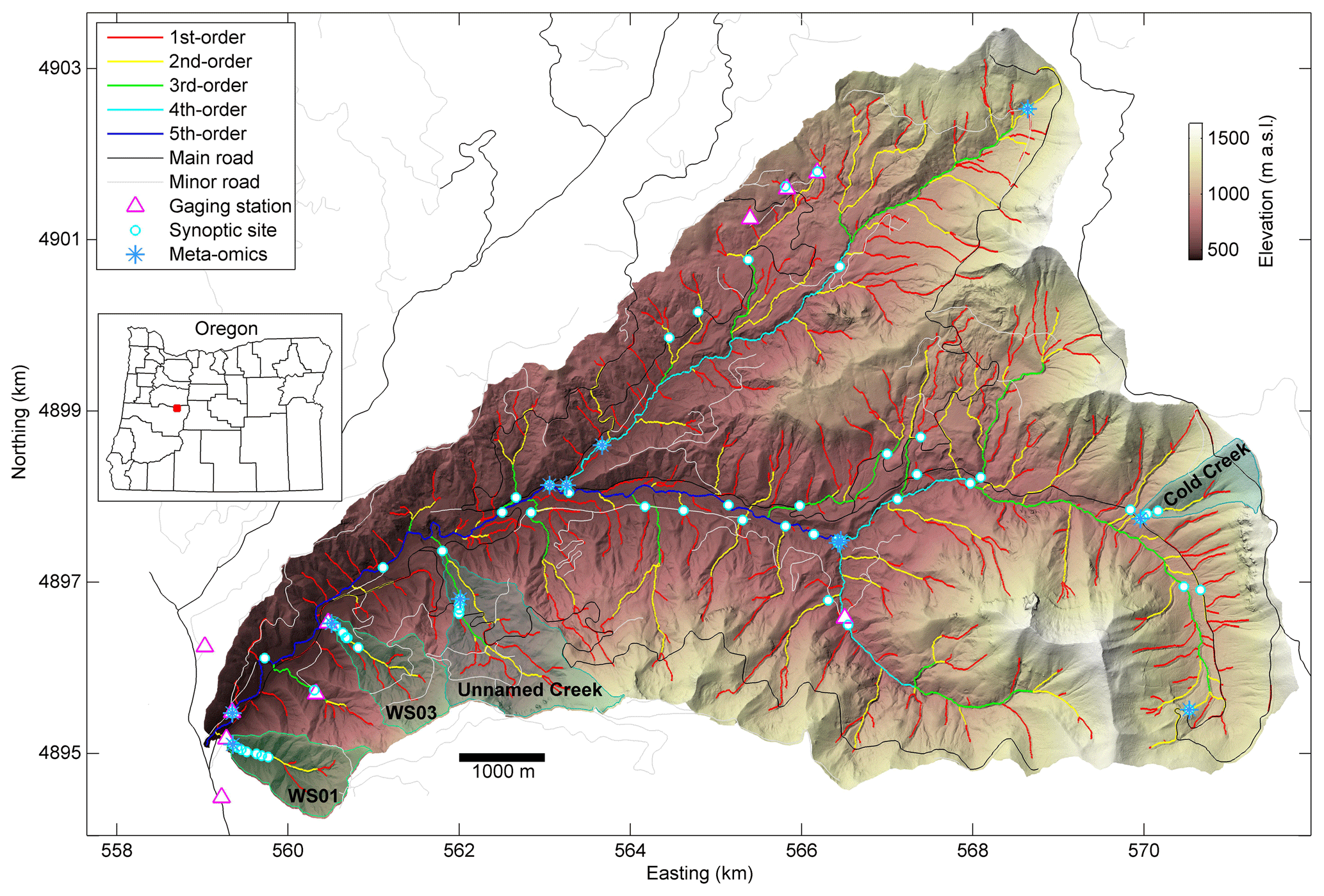
Figure 1Synoptic sites and lidar-derived stream network (see details on network definition in Sect. 3.1.1).
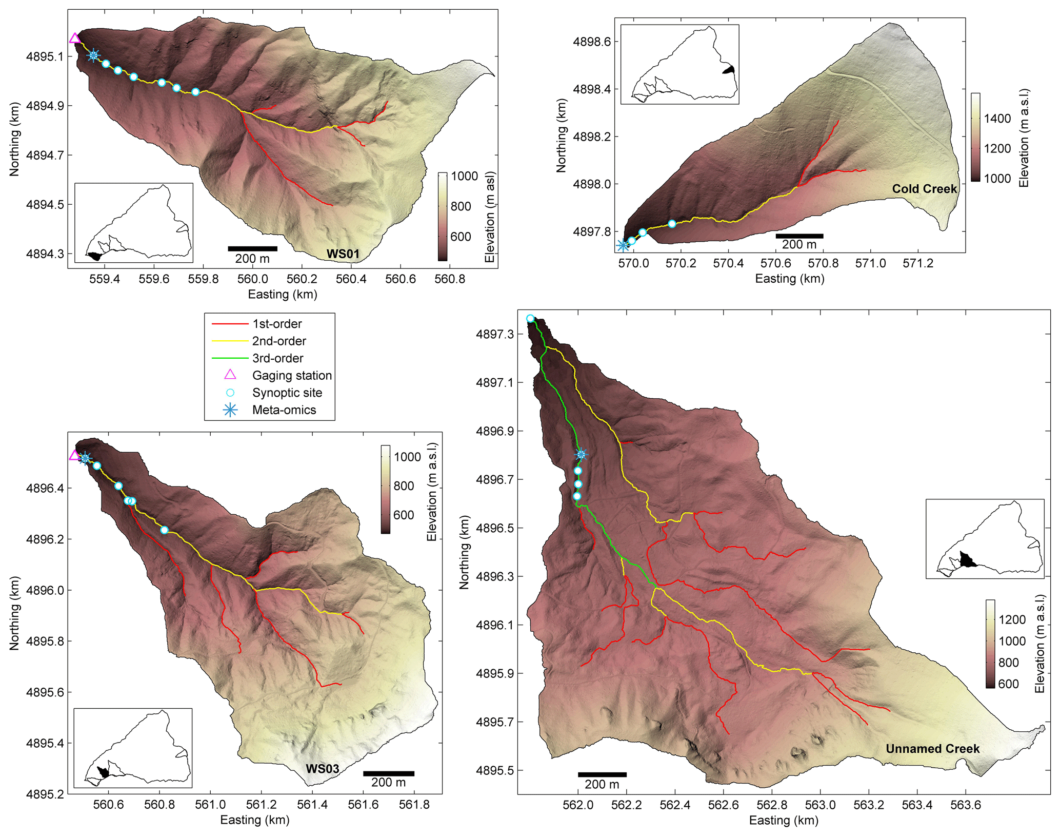
Figure 2Headwater catchments in the major landform units at the H. J. Andrews Experimental Forest, including multiple synoptic sites along an intensively studied reach. WS01 and WS03 are located in the upper Oligocene–lower Miocene basaltic flows, an unnamed creek on a deep-seated earthflow, and Cold Creek in more modern plieocascade volcanics. Characteristics of each landform and catchment are detailed in Table 1.
Table 1Summary of site characteristics for the four headwater catchments where more intensive sampling was conducted. The descriptions of these headwater catchments are considered representative of the major landform types within the HJA (after Dyrness, 1969; Swanson and James, 1975; Swanson and Jones, 2002). See catchment topography in Fig. 2 for each site.
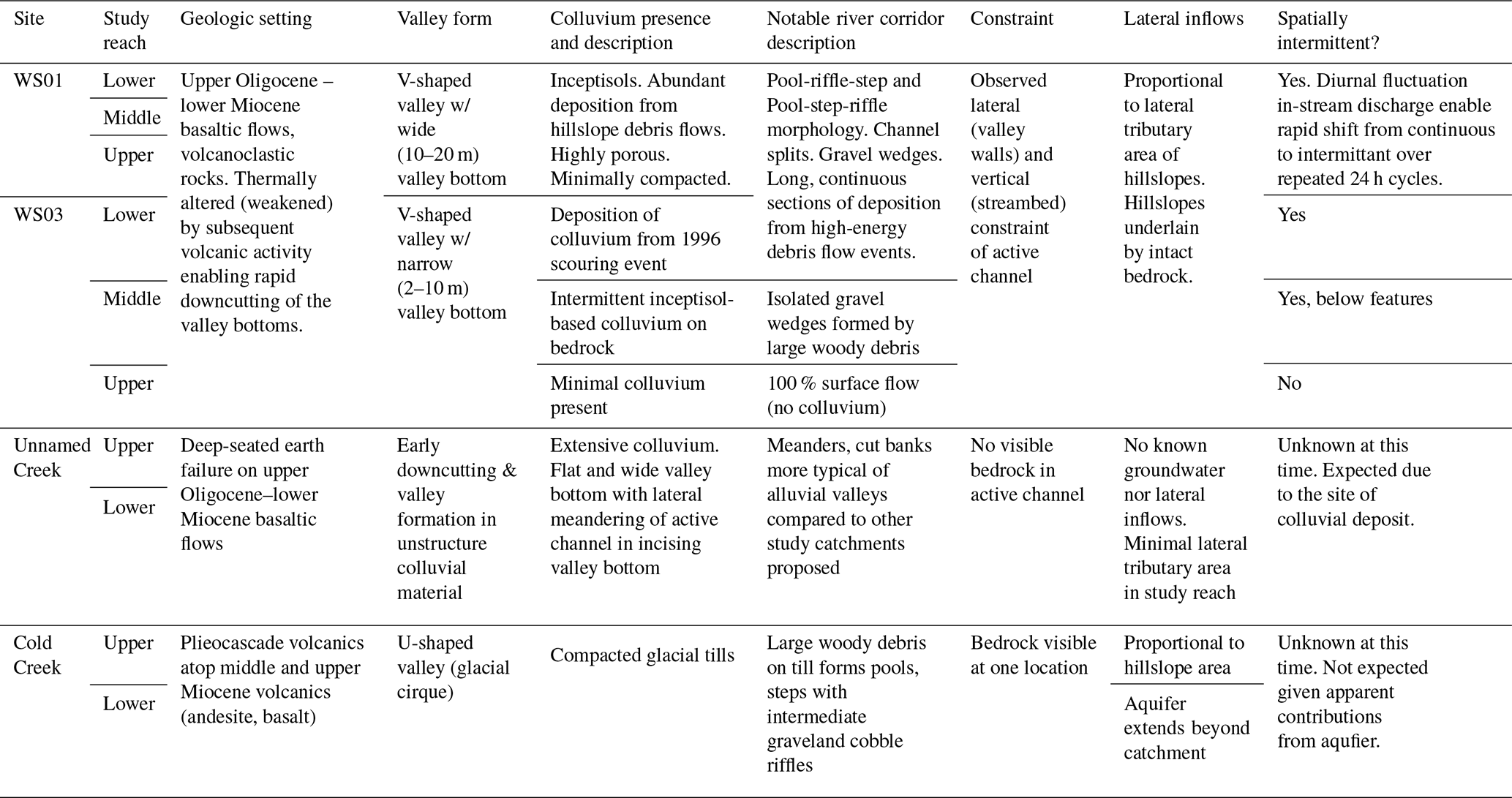
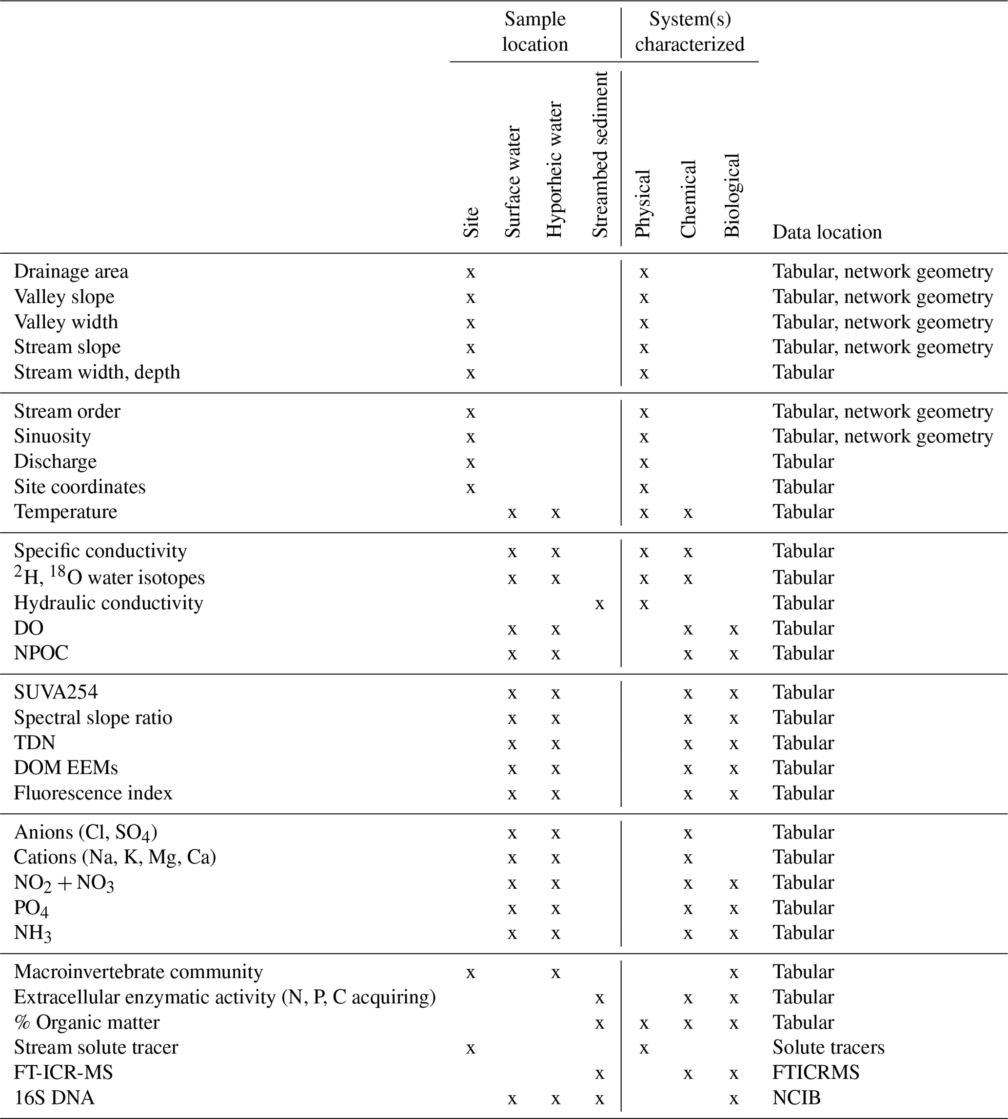
Table 2Left: Summary of sample collection (site characterization, streambed sediment, stream water, hyporheic water) and analyses included in this data set. Center: mapping of data types to their characterization of physical, chemical, and/or biological systems (after definitions of Ward, 2015). Right: data archival summary.
3.1 Synoptic site characterization
3.1.1 Topographic analysis
The stream network was derived from a 1 m digital terrain model based on airborne lidar collected in 2008 (Spies, 2016). We used the one-directional flow accumulation algorithm (Seibert and McGlynn, 2007) implemented in a modified version of TopoToolbox (Schwanghart and Kuhn, 2010; Schwanghart and Scherler, 2014) to derive the direction of flow and accumulation of drainage area within the basin. We defined the stream network as any location draining more than 5 ha. The threshold was established based on iteratively comparing the derived stream network to our experience working in headwater catchments and their extent (consistent with analyses by Ward et al., 2018). The TopoToolbox algorithm defined study reaches as the segment between two junctions. In our analysis, we defined 686 river corridor segments including a total length of about 209 km of valley containing about 242 km of stream. For each study reach, we tabulated the sinuosity of the stream within the valley. Next, we discretized each reach into 10 m segments, extracting valley slope, stream sinuosity, and stream slope for each segment (after Corson-Rikert et al., 2016; Ward et al., 2018). Each synoptic site was assigned a stream order and average valley slope, streambed slope, and sinuosity for the reach within which it was located.
3.1.2 Hydraulic and valley geometry
At each synoptic site, field observations of valley width were collected using a tape measure, with valley edge being visually defined in the field based on the hillslope break point between the relatively flat valley bottom and steeper valley walls. Total wetted channel width was measured perpendicular to the direction of flow at the synoptic site, and average channel depth was recorded based on at least five measurements of depth spaced evenly across the channel.
3.1.3 Hydraulic conductivity
At the approximate centerline of the synoptic site, a Solinst 615N drive-point piezometer (615N, Solinst Canada, Ltd., Georgetown, ON, Canada) was driven to a depth of about 65 cm below the streambed. The piezometer was screened over the distance of 50–65 cm below the streambed. The piezometer was developed and purged by pumping slowly using a peristaltic pump until the water was visually clear, typically about 5 min. Then hyporheic water sampling occurred as described below (Sect. 3.2). Then a series of three to six replicates of a falling head test were conducted using the piezometer, with water levels measured using a Van Essen Micro-Diver (DI601, Van Essen Instruments, Mukilteo, WA, USA), recording at 0.5 s intervals and corrected for any variation in atmospheric pressure collecting data every 10 min. Falling head data were used to estimate hydraulic conductivity after Hvorslev (1951). We report the geometric mean of the replicate tests for each synoptic site. Finally, we note that at five sites there was minimal (∼ < 10 cm) to no colluvium present in the valley bottom. At these sites we did not sample hyporheic water nor measure hydraulic conductivity, but we did collect streambed sediment from small in-channel deposits at the synoptic site. These sites are necessary for complete representation of the river corridor of the study catchment as there are many locations in the valley bottom that have minimal or no colluvium.
3.1.4 Macroinvertebrate community
Benthic macroinvertebrate colonization pots were installed at 44 of the 62 synoptic sites using the design of Crossman et al. (2012) during the synoptic campaign. Colonization pots were constructed of wire mesh with 1.25 cm openings formed into cylinders approximately 15 cm in height and 8 cm in diameter, including a screened bottom. Hence, at sites where surface sediment grain sizes were larger than 8 cm, they could not be installed. Substrate was excavated by hand and placed in each pot prior to installing so that the top of each pot was level with the streambed. Colonization pots remained in situ for about 6 weeks following installation. Removal was achieved by pulling a cable to raise a specially constructed tarpaulin bag around the sides of the pot before extraction, thereby minimizing sample loss. All substrate and macroinvertebrates were placed in a 90 % ethanol solution for preservation. Additionally at 10 sites, surface samples of macroinvertebrates were collected with a Surber sampler with a 330 µm mesh net, collected in triplicate at proximal locations and pooled for identification during the synoptic campaign. Surface samples were processed using identical preservation methods, and identification was conducted by the same researcher.
After separation of macroinvertebrates, sediment samples were oven-dried and sieved to assemble grain size distributions for each colonization pot. Importantly, because the pots were packed by hand in flowing water, we expect these grain size distributions are biased toward the coarse fraction of streambed sediment, as finer materials would have washed away during packing. Additionally, large cobbles would not have fit into the pots and excluded from collection.
Identification was performed under the stereomicroscope, except for the Chironomidae (family larvae and early larval instars of the Plecoptera (order) and Ephemeroptera (order)), which were mounted in the Euparal and examined under the light microscope as described by Andersen (2013). Macroinvertebrates were identified to the lowest possible taxonomic level, including the differentiation of adult and juvenile stages. Identification was performed using established keys (Merritt and Cummins, 1996; Andersen, 2013; Malicky, 1983; Langton, 1991; Epler, 2001).
3.2 Water sampling & analyses
3.2.1 Sample collection from stream and hyporheic zone
All water samples were collected using a peristaltic pump to sample water at a flow rate of about 0.5 L min−1. The pump intake was located either in the stream thalweg for surface samples or in the developed piezometer for hyporheic samples. Tubing was rinsed with water from the stream or hyporheic zone for at least 5 min prior to sample collection to minimize cross-contamination between sites. We did not record the pumping rates nor volumes for this rinse, and acknowledge it may have an impact on the flow field prior to sample collection. However, we expect this would be minimal because the sediment is generally highly hydraulically conductive.
First, water temperature and dissolved oxygen were recorded using a YSI ProODO handheld probe (YSI, Inc., Yellow Springs, OH, USA) with an optical dissolved oxygen (DO) sensor and thermistor. For stream samples, the probe was held in the water column at the synoptic site near the pump intake. For hyporheic samples, water was pumped into a small flow-through cell until it overflowed, and then the sensor was placed into the cell while flow continued. For both stream and hyporheic observations the sensor remained in place in the flowing water until probe readings for temperature and DO stabilized. Specific conductivity was also measured with a handheld conductivity probe (YSI EC300; YSI, Inc., Yellow Springs, OH, USA) using the same approaches.
Physical water samples for subsequent laboratory analyses were collected from the stream and hyporheic zone using identical methods. (1) Unfiltered samples for water isotope analysis (Sect. 3.2.2) were collected in 20 mL glass scintillation vials with conical inserts and were capped without headspace to minimize fractionation. (2) Samples for dissolved water chemistry and nutrients (Sect. 3.2.3) were collected by field filtering using handheld 65 mL syringes. Syringes were triple rinsed with sample water prior to collection of any sample volume. Samples for dissolved organic carbon (DOC) analyses were field-filtered using a 0.2 µm cellulose acetate filter. Acid-washed amber HDPE bottles were triple-rinsed with filtered sample water prior to sample collection. DOC samples were placed in a cooler with ice in the field and remained chilled until analysis. Samples for dissolved nutrients, anions, and cations were field-filtered using a 0.45 µm cellulose acetate filter. Sample bottles were triple-rinsed with filtered sample water prior to sample collection. Dissolved nutrient samples were placed on dry ice in the field immediately after collection and remained frozen until analysis. (3) Samples for microbial analysis (Sect. 3.2.4) were collected following Crevecoeur et al. (2015) by pumping water through a Sterivex (Millipore) cartridge with a 0.22 µm Durapore (PVDF) filter membrane until either 1 L of water was filtered or 45 min elapsed. Cartridges were immediately sparged to remove site water, filled with RNAlater stabilization solution (Ambion), and frozen in the field on dry ice. Samples remained frozen on dry ice until transferred and stored in a −80 ∘C freezer until analysis.
3.2.2 Water stable isotope ratios
We analyzed water stable isotopes to facilitate characterization of water ages using a cavity ring-down spectroscopy method (Picarro L2130-I, Picarro Inc.), following laboratory protocols described by Nickolas et al. (2017). Briefly, samples were run under high-precision analysis mode using a 10 µL syringe for six injections per sample. We discarded the first three injections to eliminate memory effects. We used internal standards to develop calibration equations for stable isotopes of oxygen and hydrogen. The internal standards were calibrated using primary IAEA standards for Vienna Standard Mean Ocean Water (VSMOW2: δ18O=0.0 ‰, δ2H=0.0 ‰), Standard Light Antarctic Precipitation (SLAP2: ‰, ‰), and Greenland Ice Sheet Precipitation (GIPS: ‰, ‰). All stable isotopic values were reported as delta (δ) values in parts per thousand (‰), which represent the deviation from the adopted VSMOW2 standard. Internal laboratory precision of the mean reported δ18O and δ2H values was estimated as 0.03 ‰ and 0.058 ‰ for δ18O and δ2H, respectively, based on the analysis of >50 duplicate samples. The external accuracy – representing the overall accuracy of the laboratory – was estimated as 0.058 ‰ and 0.241 ‰ for δ18O and δ2H by comparing > 60 estimated values for a known standard. A total of seven samples collected for water isotope analysis were lost due to breakage of collection vials during transport. Paired surface and hyporheic samples were recollected on 1–3 August 2016 for these locations.
3.2.3 Dissolved water chemistry and nutrients
Dissolved nutrients (, , and NH3) were analyzed on a San automated wet chemistry analyzer–segmented flow analyzer (Skalar Analytical B.V., Netherlands). Anions (Cl−, ) and cations (Na+, K+, Mg2+, Ca2+) were analyzed on a Dionex ICS5000 ion chromatography system (Thermo Fisher Scientific). Samples were thawed on the laboratory bench prior to analysis (typically 2–4 h) and were analyzed at room temperature.
DOC concentrations (as non-purgeable organic carbon, NPOC) and total dissolved nitrogen (TDN) were analyzed via acid-catalyzed high-temperature combustion using a Shimadzu TOC-L analyzer with a TN module (Shimadzu Scientific Instruments, Kyoto, Japan). Samples were allowed to come to room temperature prior to analysis.
Dissolved organic matter (DOM) optical quality was analyzed via absorbance and fluorescence spectroscopy. UV–visible absorbance spectra ranging from 220 to 800 nm were collected using semi-micro, Brand-Tech cuvettes with a 1 cm path length on a Shimadzu dual-beam UV 1800 spectrophotometer (Shimadzu Scientific Instruments, Kyoto, Japan). Samples were allowed to come to room temperature prior to analyses. E-Pure water (18 MΩ, Barnstead E-Pure system) was used as a blank and cuvettes were triplicate rinsed with E-Pure water and rinsed with sample water between readings.
Excitation-emission matrices (EEMs) were measured over excitation wavelengths of 250–450 nm and emission wavelengths of 320–550 nm on a Horiba Aqualog fluorometer (Horiba Scientific, Kyoto, Japan). Following the methods of Cory et al. (2010b), EEMs were generated for each sample using a 4 s integration time using a quartz cuvette with a 1 cm path length and E-Pure water as a blank. Samples were allowed to come to room temperature prior to analysis. Cuvettes were rinsed with E-Pure water at least 10 times and triplicate rinsed with sample water between readings. EEMs were corrected for instrument-specific excitation and emission corrections and the inner-filter effect (Cory et al., 2010). E-Pure water blank EEMs were collected and used to correct for Raman scattering. Fluorescence intensities from corrected-sample EEMs were converted to Raman units (Stedmon and Bro, 2008). EEM corrections and processing were performed using MATLAB consistent with Cory et al. (2010).
Using EEMs and UV–visible absorbance spectra, several DOM quality indices were calculated for each sample. Specific UV absorbance at 254 nm (SUVA254) was calculated using absorbance readings at 254 nm normalized for path length (m−1) and DOC concentration (mg L−1). Higher SUVA254 values are associated with higher aromaticity of DOM (Weishaar et al., 2003). Spectral slope ratio (SR) was calculated from absorbance spectra following the methods of Helms et al. (2008). SR values correspond inversely to relative DOM molecular weight. Fluorescence index (FI) was calculated following Cory and McKnight (2005) as the ratio of emission (em) intensities for 470 and 520 nm at the 370 nm excitation (ex) wavelength. FI values correspond to DOM source with lower FI values corresponding to allochthonous, terrestrially derived DOM and higher FI values corresponding to autochthonous, microbially derived DOM (McKnight et al., 2001).
Intensities of specific EEM peaks and absorbance wavelengths were selected and reported as well-documented proxies for character and sources of DOM. Following Coble (1996) and Cory and Kaplan (2012), EEM peak A (ex 250, 420/em 500) and peak C (ex 250, 365/em 466) were reported as proxies for humic-like, terrestrially derived fluorescent DOM (FDOM). EEM peak T (ex 250, 285/em 344) was reported as a proxy for protein-like FDOM (Cory and Kaplan, 2012). Specific decadic and Napierian absorption coefficients reported serve as proxies for colored DOM (CDOM), and can be used as indicators for specific sources and reactive fractions of the DOM pool (Spencer et al., 2009). Decadic absorption coefficients (m−1) were calculated from absorbance readings at specific wavelengths normalized for path length (m). Napierian absorption coefficients (m−1) are reported on a natural log scale and are calculated from absorbance readings at specific wavelengths normalized for path length (m) and multiplied by a factor of 2.303.
3.2.4 Microbial ecology
To characterize the bacterial communities collected from the surface water and hyporheic zone, we first isolated the filter membrane from the Sterivex cartridge. We extracted DNA from the filters using the DNeasy PowerWater kit (Qiagen). Following DNA extractions, we used polymerase chain reaction (PCR) to amplify the V4-V5 region of the 16S rRNA gene using barcoded primers (515F and 806R) designed for the Illumina MiSeq sequencing platform (Caporaso et al., 2012). The sequence libraries were cleaned using the AMPure XP purification kit (Agencourt) and quantified using the PicoGreen dsDNA quantification kit (Quant-iT, Invitrogen). Libraries were pooled at 10 ng per library. Pooled DNA libraries were sequenced on the Illumina MiSeq platform at the Center for Genomics and Bioinformatics sequencing facility at Indiana University using paired-end reads (Illumina Reagent Kit v2, 500-reaction kit).
3.3 Sediment sampling & analyses
3.3.1 Sample collection
Streambed sediment samples were collected near the piezometer at each synoptic site. Sample collection involved manually removing the armor layer from the bed and then using a small specimen cup and putty knife to remove bed sediment without loss of fines. Samples were sieved to remove coarse material using a 2 mm sieve. Sieved material was placed in a sterile 50 mL centrifuge tube and frozen on dry ice immediately after collection. Samples were retained on dry ice or in a −80 ∘C freezer until analysis. Duplicate sediment samples were collected for analysis of extracellular enzymatic activity at nine sites. Samples collected in this fashion were used for extracellular enzymatic activity and Fourier transform ion cyclotron resonance mass spectrometry (FT-ICR-MS) analyses, detailed in subsequent sections.
Table 3Enzymes examined in this study and the reactions they catalyze.

1 MUF: 4-methylumbelliferyl. 2 AMC: 7-amino-4-methylcoumarin.
3.3.2 Extracellular enzymatic activity
Enzyme activities were determined using laboratory assays in which sediment extracts were exposed to model substrates that are hydrolyzed by the enzymes (Table 3). Protocols were based on those described by Sinsabaugh et al. (1997) and Belanger et al. (1997). Frozen sediment samples were thawed to room temperature and then 10 mL of 5 mM sodium bicarbonate buffer solution was added to approximately 1 mL subsamples of sediment in 15 mL centrifuge tubes. These tubes were homogenized with a vortex mixer for 15 s and then centrifuged for 15 min at 400 g. Samples were then stored in a refrigerator overnight and the following day 200 µL of the supernatant was pipetted in triplicate onto 96-well microplates. To ensure that any increase in fluorescence was due to enzyme activity, a set of control samples which had been boiled for 5 min to denature enzymes was also added to the plates. A set of standard solutions with known concentrations of fluorescent product were also added to each plate to generate a standard curve.
Background fluorescence readings were recorded and substrate solution was added to start the enzyme reaction. Each well in the microplate received 50 µL of a 200 µM substrate solution. Fluorescence measurements (440 nm emission intensity and 365 nm excitation wavelength) were recorded every ∼ 30 min for at least 3 h. Microplates were protected from light and kept at room temperature between readings. Fluorescence was measured using a BioTek Synergy Mx microplate reader. The accumulation of fluorescent products (AMC or MUF; see Table 3) from the hydrolysis reactions was measured over time and enzyme activity was calculated as the slope of a regression of AMC or MUF concentration against time.
About 1 mL of each sediment sample was dried, weighed, and then combusted at 550 ∘C and reweighed to determine ash-free dry mass (AFDM) and percent organic content for the sample (Wallace et al., 2006). Extracellular enzymatic activity rates were then normalized to organic matter content and are reported in units of µmol g AFDM−1 h−1.
3.3.3 Organic matter characterization
FT-ICR-MS solvent extraction and data acquisition
We performed electrospray ionization (ESI) and Fourier transform ion cyclotron resonance (FT-ICR) mass spectrometry (MS) using a 12 Tesla Bruker solariX FT-ICR-MS instrument located at the Environmental Molecular Sciences Laboratory (EMSL) in Richland, WA, USA. Prior to mass spectrometry, organic matter was extracted from sediments by adding 1 mL of water (18 MΩ ionic purity) to 500 mg of sediments (after Tfaily et al., 2017). Each sediment sample was extracted three times with the above procedure. Supernatant from all extractions was combined and diluted to 5 mL to generate a final aliquot for analysis. These aliquots were acidified to pH 2 with 85 % phosphoric acid and extracted with PPL cartridges (Bond Elut), following Dittmar et al. (2008). We performed weekly calibration after Tfaily et al. (2017) and instrument settings were optimized using Suwannee River Fulvic Acid (IHSS). The instrument was flushed between samples using a mixture of water and methanol. Blanks were analyzed at the beginning and the end of the day to monitor for background contaminants.
Samples were injected directly into the mass spectrometer and the ion accumulation time was set to 0.1 s. Data were collected from 98 to 900 at 4M, yielding 144 scans that were co-added. A standard Bruker ESI source was used to generate negatively charged molecular ions. Samples were introduced to the ESI source equipped with a fused silica tube (30 µm i.d.) through an Agilent 1200 series pump (Agilent Technologies) at a flow rate of 3.0 µL min−1. Experimental conditions were as follows: needle voltage of +4.4 kV; Q1 set to 50 ; and the heated resistively coated glass capillary operated at 180 ∘C.
FT-ICR-MS data processing
A total of 144 individual scans were averaged for each sample and internally calibrated using an organic matter homologous series separated by 14 Da (−CH2 groups). The mass measurement accuracy was less than 1 ppm for singly charged ions across a broad range (100–1200 ). The mass resolution was ∼ 240 K at 341 . The transient was 0.8 s. Data analysis software (BrukerDaltonik version 4.2) was used to convert raw spectra to a list of values applying FTMS peak picker module with a signal-to-noise ratio (S N) threshold set to 7 and absolute intensity threshold to the default value of 100. Peaks were treated as presence/absence data because peak intensity differences are reflective of ionization efficiency as well as relative abundance (Kujawinski and Behn, 2006; Minor et al., 2012; Tfaily et al., 2015, 2017).
Putative chemical formulae were then assigned using in-house software following the compound identification algorithm (CIA), proposed by Kujawinski and Behn (2006), modified by Minor et al. (2012), and previously described in Tfaily et al. (2017). Chemical formulae were assigned based on the following criteria: S N > 7, and mass measurement error < 1 ppm, taking into consideration the presence of C, H, O, N, S, and P and excluding other elements. To ensure consistent formula assignment, we aligned all sample peak lists for the entire dataset to each other in order to facilitate consistent peak assignments and eliminate possible mass shifts that would impact formula assignment. We implemented the following rules to further ensure consistent formula assignment: (1) we consistently picked the formula with the lowest error and with the lowest number of heteroatoms and (2) the assignment of one phosphorus atom requires the presence of at least four oxygen atoms.
The chemical character of thousands of peaks in each sample's ESI FT-ICR-MS spectrum was evaluated on van Krevelen diagrams. Compounds were plotted on the van Krevelen diagram on the basis of their molar H : C ratios (y axis) and molar O : C ratios (x axis) (Kim et al., 2003). Van Krevelen diagrams provide a means to visualize and compare the average properties of organic compounds and assign compounds to the major biochemical classes (e.g., lipid, protein, lignin, carbohydrate, and condensed aromatic). In this study, biochemical compound classes are reported as relative abundance values based on counts of C, H, and O for the following H : C and O : C ranges: lipids (0 < O : C ≤ 0.3, 1.5 ≤ H : C ≤ 2.5), unsaturated hydrocarbons (0 ≤ O : C ≤ 0.125, 0.8 ≤ H : C < 2.5), proteins (0.3 < O : C ≤ 0.55, 1.5 ≤ H : C ≤ 2.3), amino sugars (0.55 < O : C ≤ 0.7, 1.5 ≤ H : C ≤ 2.2), lignin (0.125 < O : C ≤ 0.65, 0.8 ≤ H : C < 1.5), tannins (0.65 < O : C ≤ 1.1, 0.8 ≤ H : C < 1.5), and condensed hydrocarbons (0 ≤ 200 O : C ≤ 0.95, 0.2 ≤ H : C < 0.8) (Tfaily et al., 2015).
Finally, we calculated the Gibbs free energy of OC oxidation under standard conditions (ΔGoCox) from the nominal oxidation state of carbon (NOSC) after La Rowe and Van Cappellen (2011). Though the exact calculation of ΔGoCox necessitates an accurate quantification of all species involved in every chemical reaction in a sample, the use of NOSC as a practical basis for determining ΔGoCox has been validated (Arndt et al., 2013; LaRowe and Van Cappellen, 2011; Graham et al., 2017; Boye et al., 2017; Stegen et al., 2018).
3.4 Stream solute tracer
Two injections of a conservative solute tracer (NaCl) were conducted at 46 synoptic sites, one each at the upstream and downstream reach boundaries to quantify discharge and short-term hyporheic flux. First, we fixed the upstream end of the study reach at the same transect as the piezometer and sampling location. Next, we set the downstream station at a distance of about 20 wetted channel widths downstream from the piezometer and sampling location, a length selected to capture a representative valley segment (after Anderson et al., 2005). Minor variation in distance was allowed to place two specific conductivity sensors in well-mixed locations within the stream channel, with the total length reported for each tracer study reach. For each injection, mixing lengths for the solute tracer were visually estimated (after Payn et al., 2009; Ward et al., 2013b, a), and small releases of a visual tracer were used to confirm mixing lengths when visual estimates were uncertain. A known mass of NaCl was dissolved in stream water and released as an instantaneous injection one mixing length upstream from the reach boundary. Initially, the downstream slug was released and measured only at the downstream location to enable dilution gauging estimates of discharge at the downstream end of the study reach. Next, the upstream slug was released and monitored at both locations to enable dilution gauging at the upstream transect, and evaluation of both recovered and lost tracer along the study reach. The experimental design closely follows Payn et al. (2009) and Ward et al. (2013b).
Solute tracer data at the reach boundaries were recorded as specific conductance (Onset Computer Corporation, Bourne, MA, USA). We used a four-point calibration curve constructed by dissolving known masses of NaCl in stream water to convert specific conductance to salt concentration (C = 0.5022 S, where C is NaCl concentration in milligrams per liter and S is specific conductance; r2>0.99). Notably, this equation does not include a y intercept as we first subtracted background S from all observations prior to conversion. In addition to providing the full solute tracer time series in the data set, we also provide estimates of discharge (Q) based on dilution gauging, truncating the recovered tracer time series after 99 % recovery (after Mason et al., 2012; Ward et al., 2013b, a). We report in the data set Q for both the upstream and downstream ends of the study reach, and the change in Q along the study reach. Several additional metrics describing solute tracer time series are detailed in Ward et al. (2019).
These data are archived in the Consortium of Universities for the Advancement of Hydrologic Science, Inc. (CUAHSI) HydroShare data repository, accessible as https://doi.org/10.4211/hs.f4484e0703f743c696c2e1f209abb842 (Ward, 2019). In addition to tabular data, time series for solute tracer experiments and detailed results from the FT-ICR-MS analyses are archived. Raw sequence data for 16S DNA analyses are archived at the U.S. National Center for Biotechnology Information (NCBI) as a BioProject (Accession: PRJNA534507).
We provide here a detailed characterization of physical, chemical, and biological parameters that are germane to the study of river corridor exchange and associated ecosystem functions and services. These data represent state-of-the-science characterization conducted at a heretofore unpresented resolution in space, and the only known data set that integrates across physical, chemical, and biological dimensions of the river corridor, including coverage across 5 stream orders. Taken together, these data will enable the testing of hypothesized processes and relationships in the river corridor across spatial scales, and will be useful in the generation of testable hypotheses about river corridor exchanges in future studies.
All co-authors participated in the field collection, laboratory analysis, and/or curation of the data set. ASW was primarily responsible for the writing of this paper and assembly of the archival database. ASW and JPZ conceived of the study design with input from all co-authors. All authors contributed to the writing of this paper.
The authors declare that they have no conflict of interest.
This article is part of the special issue “Linking landscape organisation and hydrological functioning: from hypotheses and observations to concepts, models and understanding (HESS/ESSD inter-journal SI)”. It is not associated with a conference.
Data and facilities were provided by the H. J. Andrews Experimental Forest and Long Term Ecological Research program, administered cooperatively by the USDA Forest Service Pacific Northwest Research Station, Oregon State University, and the Willamette National Forest. Adam S. Ward's time in preparation of this paper was supported by the University of Birmingham's Institute of Advanced Studies. A portion of the research was performed using EMSL (grid 436923.9), a DOE Office of Science User Facility sponsored by the Office of Biological and Environmental Research. Finally, the authors acknowledge this would not have been possible without support from their home institutions.
This research has been supported by the Leverhulme Trust (“Where rivers, groundwater and disciplines meet: a hyporheic research network”), the UK Natural Environment Research Council (grant no. NE/L003872/1), the U.S. Department of Energy (Pacific Northwest National Laboratory, grant no. DE-SC0019377), the National Science Foundation (grant nos. DEB-1440409, EAR-1652293, EAR-1417603, and EAR-1446328), the University of Birmingham (grant no. Institute of Advanced Studies), and the European Commission (HiFreq, grant no. 734317).
This paper was edited by Loes van Schaik and reviewed by Eric Moore and one anonymous referee.
Abbott, B. W., Gruau, G., Zarnetske, J. P., Moatar, F., Barbe, L., Thomas, Z., Fovet, O., Kolbe, T., Gu, S., Pierson-Wickmann, A. C., Davy, P., and Pinay, G.: Unexpected spatial stability of water chemistry in headwater stream networks, Ecol. Lett., 21, 296–308, https://doi.org/10.1111/ele.12897, 2018.
Anderson, J. K., Wondzell, S. M., Gooseff, M. N., and Haggerty, R.: Patterns in stream longitudinal profiles and implications for hyporheic exchange flow at the H. J. Andrews Experimental Forest, Oregon, USA, Hydrol. Process., 19, 2931–2949, 2005.
Andersen, T.: in: Chironomidae of the Holarctic Region: Keys and Diagnoses: Larvae, edited by: Andersen, T., Cranston, P. S., and Epler, J. H., Scandinavian Society of Entomologym, 2013.
Arndt, S., Jørgensen, B. B., LaRowe, D. E., Middelburg, J. J., Pancost, R. D., and Regnier, P.: Quantifying the degradation of organic matter in marine sediments: A review and synthesis, Earth-Sci. Rev., 123, 53–86, https://doi.org/10.1016/j.earscirev.2013.02.008, 2013.
Belanger, C., Desrosiers, B., and Lee, K.: Microbial extracellular enzyme activity in marine sediments: extreme pH to terminate reaction and sample storage, Aquat. Microb. Ecol., 13, 187–196, 1997.
Bernhardt, E. S., Blaszczak, J. R., Ficken, C. D., Fork, M. L., Kaiser, K. E., and Seybold, E. C.: Control Points in Ecosystems: Moving Beyond the Hot Spot Hot Moment Concept, Ecosystems, 20, 665–682, https://doi.org/10.1007/s10021-016-0103-y, 2017.
Boano, F., Harvey, J. W., Marion, A., Packman, A. I., Revelli, R., Ridolfi, L., and Worman, A.: Hyporheic flow and transport processes: Mechanisms, models, and biogeochemical implications, Rev. Geophys., 52, 603–679, https://doi.org/10.1002/2012RG000417, 2014.
Boulton, A. J., Findlay, S., Marmonier, P., Stanley, E. H., and Valett, H. M.: The functional significance of the hyporheic zone in streams and rivers, Annu. Rev. Ecol. Syst., 29, 59–81, 1998.
Boye, K., Noël, V., Tfaily, M. M., Bone, S. E., Williams, K. H., Bargar, J. R., and Fendorf, S.: Thermodynamically controlled preservation of organic carbon in floodplains, Nat. Geosci., 10, 415–419, https://doi.org/10.1038/ngeo2940, 2017.
Brunke, M. and Gonser, T.: The ecological significance of exchange processes between rivers and groundwater, Freshw. Biol., 37, 1–33, 1997.
Caporaso, J. G., Lauber, C. L., Walters, W. A., Berg-Lyons, D., Huntley, J., Fierer, N., Owens, S. M., Betley, J., Fraser, L., Bauer, M., Gormley, N., Gilbert, J. A., Smith, G., and Knight, R.: Ultra-high-throughput microbial community analysis on the Illumina HiSeq and MiSeq platforms, ISME J., 6, 1621–1624, https://doi.org/10.1038/ismej.2012.8, 2012.
Coble, P. G.: Characterization of marine and terrestrial DOM in seawater using excitation-emission matrix spectroscopy, Mar. Chem., 51, 325–346, https://doi.org/10.1016/0304-4203(95)00062-3, 1996.
Corson-Rikert, H. A., Wondzell, S. M., Haggerty, R., and Santelmann, M. V: Carbon dynamics in the hyporheic zone of a headwater mountain streamin the Cascade Mountains, Oregon, Water Resour. Res., 52, 7556–7576, https://doi.org/10.1029/2008WR006912.M, 2016.
Cory, R. M. and Kaplan, L. A.: Biological lability of streamwater fluorescent dissolved organic matter, Limnol. Oceanogr., 57, 1347–1360, https://doi.org/10.4319/lo.2012.57.5.1347, 2012.
Cory, R. M. and McKnight, D. M.: Fluorescence spectroscopy reveals ubiquitous presence of oxidized and reduced quinones in dissolved organic matter, Environ. Sci. Technol., 39, 8142–8149, https://doi.org/10.1021/es0506962, 2005.
Cory, R. M., Miller, M. P., McKnight, D. M., Guerard, J. J., and Miller, P. L.: Effect of instrument-specific response on the analysis of fulvic acid fluorescence spectra, Limnol. Oceanogr.-Meth., 8, 67–78, https://doi.org/10.4319/lom.2010.8.67, 2010.
Crevecoeur, S., Vincent, W. F., Comte, J., and Lovejoy, C.: Bacterial community structure across environmental gradients in permafrost thaw ponds: methanotroph-rich ecosystems, Front. Microbiol., 6, 192, https://doi.org/10.3389/fmicb.2015.00192, 2015.
Crossman, J., Bradley, C., Milner, A., and Pinay, G.: Influence Of Environmental Instability Of Groundwater-Fed Streams On Hyporheic Fauna, On A Glacial Floodplain, Denali National Park, ALASKA, River Res. Appl., 29, 548–559, https://doi.org/10.1002/rra.1619, 2012.
Deligne, N. I., Mckay, D., Conrey, R. M., Grant, G. E., Johnson, E. R., O'Connor, J., and Sweeney, K.: Field-trip guide to mafic volcanism of the Cascade Range in Central Oregon – A volcanic, tectonic, hydrologic, and geomorphic journey, Sci. Investig. Rep., 110, https://doi.org/10.3133/sir20175022H, 2017.
Dent, C. L. and Grimm, N. B.: Spatial heterogeneity of stream water nutrient concentrations over successional time, Ecology, 80, 2283–2298, https://doi.org/10.1890/0012-9658(1999)080[2283:SHOSWN]2.0.CO;2, 1999.
Dittmar, T., Koch, B., Hertkorn, N., and Kattner, G.: A simple and efficient method for the solid-phase extraction of dissolved organic matter (SPE-DOM) from seawater, Limnol. Oceanogr.-Meth., 6, 230–235, https://doi.org/10.4319/lom.2008.6.230, 2008.
Dupas, R., Minaudo, C., and Abbott, B. W.: Stability of spatial patterns in water chemistry across temperate ecoregions, Environ. Res. Lett., 14, 074015, https://doi.org/10.1088/1748-9326/ab24f4, 2019.
Dyrness, C. T.: Hydrologic properties of soils on three small watersheds in the western Cascades of Oregon, USDA For. SERV RES NOTE PNW-111, 17 pp., 1969.
Epler, J. H. Identification manual for the larval Chironomidae (Diptera) of North and South Carolina, A guide to the taxonomy of the midges of the southeastern United States, including Florida. Special Publication SJ2001-SP13. North Carolina Department of Environment and Natural Resources, Raleigh, NC, and St. Johns River Water Management District, Palatka, FL, 526 pp., 2001.
Graham, E. B., Tfaily, M. M., Crump, A. R., Goldman, A. E., Bramer, L. M., Arntzen, E., Romero, E., Resch, C. T., Kennedy, D. W., and Stegen, J. C.: Carbon Inputs From Riparian Vegetation Limit Oxidation of Physically Bound Organic Carbon Via Biochemical and Thermodynamic Processes, J. Geophys. Res.-Biogeo., 122, 3188–3205, https://doi.org/10.1002/2017JG003967, 2017.
Hale, R. L. and Godsey, S. E.: Dynamic stream network intermittence explains emergent dissolved organic carbon chemostasis in headwaters, Hydrol. Process., 33, 1926–1936, https://doi.org/10.1002/hyp.13455, 2019.
Harvey, J. W. and Gooseff, M. N.: River corridor science: Hydrologic exchange and ecological consequences from bedforms to basins, Water Resour. Res., 51, 6893–6922, https://doi.org/10.1002/2015WR017617, 2015.
Helms, J. R., Stubbins, A., Ritchie, J. D., Minor, E. C., Kieher, D. J., and Mopper, K.: Absorption spectral slopes and slope ratios as indicators of molecular weight, source, and photobleaching of chromophoric dissolved organic matter, Limnol. Oceanogr., 53, 955–969, https://doi.org/10.1186/s12913-017-2639-8, 2008.
Hvorslev, M. J.: Time lag and soil permeability in ground-water observations. Bulletin No. 36, Waterways Exper. Sta., Corps of Engineers, U.S. Army, Vicksburg, Mississippi, 50 pp., 1951.
Isaak, D. J., Peterson, E. E., Ver Hoef, J. M., Wenger, S. J., Falke, J. A., Torgersen, C. E., Sowder, C., Steel, E. A., Fortin, M.-J., Jordan, C. E., Ruesch, A. S., Som, N., and Monestiez, P.: Applications of spatial statistical network models to stream data, WIREs Water, 1, 277–294, https://doi.org/10.1002/wat2.1023, 2014.
Jefferson, A., Grant, G. E., and Lewis, S. L.: A River Runs Underneath It: Geological Control of Spring and Channel Systems and Management Implications, Cascade Range, Oregon, in: Advancing the Fundamental Sciences Proceedings of the Forest Service: Proceedings of the Forest Service National Earth Sciences Conference, 1, 18–22, 2004.
Johnson, S. L.: Factors influencing stream temperatures in small streams: substrate effects and a shading experiment, Can. J. Fish. Aquat. Sci., 61, 913–923, 2004.
Kaufmann, P. R., Herlihy, A. T., Mitch, M. E., Messer, J. J., and Overton, W. S.: Stream chemistry in the eastern United States: 1. Synoptic survey design, acid-base status, and regional patterns, Water Resour. Res., 27, 611–627, https://doi.org/10.1029/90WR02767, 1991.
Kim, S., Kramer, R. W., and Hatcher, P. G.: Graphical Method for Analysis of Ultrahigh-Resolution Broadband Mass Spectra of Natural Organic Matter, the Van Krevelen Diagram, Anal. Chem., 75, 5336–5344, https://doi.org/10.1021/ac034415p, 2003.
Krause, S., Hannah, D. M., Fleckenstein, J. H., Heppell, C. M., Kaeser, D. H., Pickup, R., Pinay, G., Robertson, A. L., and Wood, P. J.: Inter-disciplinary perspectives on processes in the hyporheic zone, Ecohydrology, 4, 481–499, 2011.
Krause, S., Lewandowski, J., Grimm, N. B., Hannah, D. M., Pinay, G., McDonald, K., Martí, E., Argerich, A., Pfister, L., Klaus, J., Battin, T., Larned, S. T., Schelker, J., Fleckenstein, J., Schmidt, C., Rivett, M. O., Watts, G., Sabater, F., Sorolla, A., and Turk, V.: Ecohydrological interfaces as hot spots of ecosystem processes, Water Resour. Res., 53, 6359–6376, https://doi.org/10.1002/2016WR019516, 2017.
Kujawinski, E. B. and Behn, M. D.: Automated analysis of electrospray ionization fourier transform ion cyclotron resonance mass spectra of natural organic matter, Anal. Chem., 78, 4363–4373, https://doi.org/10.1021/ac0600306, 2006.
Langton, P. H.: A key to pupal exuaviae of West Palaearctic Chironomidae, Langton, 1991.
La Rowe, D. E. and Van Cappellen, P.: Degradation of natural organic matter: A thermodynamic analysis, Geochim. Cosmochim. Acta, 75, 2030–2042, https://doi.org/10.1016/j.gca.2011.01.020, 2011.
Lee-Cullin, J. A., Zarnetske, J. P., Ruhala, S. S., and Plont, S.: Toward measuring biogeochemistry within the stream-groundwater interface at the network scale: An initial assessment of two spatial sampling strategies, Limnol. Oceanogr.-Meth., 16, 722–733, https://doi.org/10.1002/lom3.10277, 2018.
Likens, G. E. and Buso, D. C.: Variation in streamwater chemistry throughout the Hubbard Brook Valley, Biogeochemistry, 78, 1–30, https://doi.org/10.1007/s10533-005-2024-2, 2006.
Lowe, W. H., Likens, G. E., and Power, M. E.: Linking Scales in Stream Ecology, Bioscience, 56, 591–597, https://doi.org/10.1641/0006-3568(2006)56[591:LSISE]2.0.CO;2, 2006.
Malicky, H.: Atlas der europäischen Köcherfliegen, vol. 24, Dr. W. Junk Publishing Company, 1983.
Mason, S. J. K., McGlynn, B. L., and Poole, G. C.: Hydrologic response to channel reconfiguration on Silver Bow Creek, Montana, J. Hydrol., 438–439, 125–136, 2012.
McDonnell, J. J., Sivapalan, M., Vache, K., Dunn, S., Grant, G. E., Haggerty, R., Hinz, C., Hooper, R. P., Kirchner, J., and Roderick, M. L.: Moving beyond heterogeneity and process complexity: A new vision for watershed hydrology, Water Resour. Res., 43, W07301, https://doi.org/10.1029/2006WR005467, 2007.
McGuire, K. J., Torgersen, C. E., Likens, G. E., Buso, D. C., Lowe, W. H., and Bailey, S. W.: Network analysis reveals multiscale controls on streamwater chemistry, P. Natl. Acad. Sci. USA, 111, 7030–7035, https://doi.org/10.1073/pnas.1404820111, 2014.
McKnight, D. M., Boyer, E. W., Westerhoff, P. K., Doran, P. T., Kulbe, T., and Andersen, D. T.: Spectrofluorometric characterization of dissolved organic matter for indication of precursor organic material and aromaticity, Limnol. Oceanogr., 46, 38–48, https://doi.org/10.4319/lo.2001.46.1.0038, 2001.
Merritt, R. W. and Cummins, K. W. (Eds.): An introduction to the aquatic insects of North America, Kendall Hunt Publishing, 1996.
Minor, E. C., Steinbring, C. J., Longnecker, K., and Kujawinski, E. B.: Characterization of dissolved organic matter in Lake Superior and its watershed using ultrahigh resolution mass spectrometry, Org. Geochem., 43, 1–11, https://doi.org/10.1016/j.orggeochem.2011.11.007, 2012.
Nickolas, L. B., Segura, C., and Brooks, J. R.: The influence of lithology on surface water sources, Hydrol. Process., 31, 1913–1925, https://doi.org/10.1002/hyp.11156, 2017.
Payn, R. A., Gooseff, M. N., McGlynn, B. L., Bencala, K. E., and Wondzell, S. M.: Channel water balance and exchange with subsurface flow along a mountain headwater stream in Montana, United States, Water Resour. Res., 45, W11427, https://doi.org/10.1029/2008WR007644, 2009.
Schwanghart, W. and Kuhn, N. J.: TopoToolbox: A set of Matlab functions for topographic analysis, Environ. Model. Softw., 25, 770–781, https://doi.org/10.1016/j.envsoft.2009.12.002, 2010.
Schwanghart, W. and Scherler, D.: Short Communication: TopoToolbox 2 – MATLAB-based software for topographic analysis and modeling in Earth surface sciences, Earth Surf. Dynam., 2, 1–7, https://doi.org/10.5194/esurf-2-1-2014, 2014.
Seibert, J. and McGlynn, B. L.: A new triangular multiple flow direction algorithm for computing upslope areas from gridded digital elevation models, Water Resour. Res., 43, 1–8, https://doi.org/10.1029/2006WR005128, 2007.
Sinsabaugh, R. L., Findlay, S., Franchini, P., and Fischer, D.: Enzymatic analysis of riverine bacterioplankton production, Limnol. Oceanogr., 42, 29–38, https://doi.org/10.4319/lo.1997.42.1.0029, 1997.
Spencer, R. G. M., Aiken, G. R., Butler, K. D., Dornblaser, M. M., Striegl, R. G., and Hernes, P. J.: Utilizing chromophoric dissolved organic matter measurements to derive export and reactivity of dissolved organic carbon exported to the Arctic Ocean: A case study of the Yukon River, Alaska, Geophys. Res. Lett., 36, L06401, https://doi.org/10.1029/2008GL036831, 2009.
Spies, T.: LiDAR Data (August 2008) for the Andrews Experimental Forest and Willamette National Forest Study Areas, HJA Data Identifier GI010, Long-term Ecol. Res., For. Sci. Data Bank, Corvalliss, Oreg. (Database), available at: http://andlter.forestry.oregonstate.edu/data/abstract.aspx?dbcode=GI010 (last access: 17 July 2018), 2016.
Stedmon, C. A. and Bro, R.: Characterizing dissolved organic matter fluorescence with parallel factor analysis: A tutorial, Limnol. Oceanogr.-Meth., 6, 572–579, https://doi.org/10.4319/lom.2008.6.572, 2008.
Stegen, J. C., Johnson, T., Fredrickson, J. K., Wilkins, M. J., Konopka, A. E., Nelson, W. C., Arntzen, E. V., Chrisler, W. B., Chu, R. K., Fansler, S. J., Graham, E. B., Kennedy, D. W., Resch, C. T., Tfaily, M., and Zachara, J.: Influences of organic carbon speciation on hyporheic corridor biogeochemistry and microbial ecology, Nat. Commun., 9, 1034, https://doi.org/10.1038/s41467-018-03572-7, 2018.
Swanson, F. J. and James, M. E.: Geology and geomorphology of the H.J. Andrews Experimental Forest, western Cascades, Oregon, Portland, OR, 1975.
Swanson, F. J. and Jones, J. A.: Geomorphology and hydrology of the HJ Andrews experimental forest, Blue River, Oregon, F. Guid. to Geol. Process. Cascadia, 36, 289–314, 2002.
Temnerud, J. and Bishop, K.: Spatial variation of streamwater chemistry in two Swedish boreal catchments: Implications for environmental assessment, Environ. Sci. Technol., 39, 1463–1469, https://doi.org/10.1021/es040045q, 2005.
Tfaily, M. M., Chu, R. K., Tolić, N., Roscioli, K. M., Anderton, C. R., Paša-Tolić, L., Robinson, E. W., and Hess, N. J.: Advanced solvent based methods for molecular characterization of soil organic matter by high-resolution mass spectrometry, Anal. Chem., 87, 5206–5215, https://doi.org/10.1021/acs.analchem.5b00116, 2015.
Tfaily, M. M., Chu, R. K., Toyoda, J., Tolić, N., Robinson, E. W., Paša-Tolić, L., and Hess, N. J.: Sequential extraction protocol for organic matter from soils and sediments using high resolution mass spectrometry, Anal. Chim. Acta, 972, 54–61, https://doi.org/10.1016/j.aca.2017.03.031, 2017.
Tonina, D. and Buffington, J. M.: Hyporheic exchange in mountain rivers I: mechanics and environmental effects, Geogr. Compass, 3, 1063–1086, https://doi.org/10.1111/j.1749-8198.2009.00226.x, 2009.
Wallace, J. B., Hutchens Jr., J. J., and Grubaugh, J. W.: Transport and storage of FPOM, in: Methods in Stream Ecolgoy, edited by: Hauer, F. R. and Lamberti, G. A., 2nd edn., Elsevier, New York, 249–271 2006.
Ward, A. S.: The evolution and state of interdisciplinary hyporheic research, WIREs Water, 3, 83–103, https://doi.org/10.1002/wat2.1120, 2015.
Ward, A. S.: ESSD 2019 – Data Collection, HydroShare, https://doi.org/10.4211/hs.f4484e0703f743c696c2e1f209abb842, 2019.
Ward, A. S. and Packman, A. I.: Advancing our predictive understanding of river corridor exchange, WIREs Water, 6, e1327, 17 pp., https://doi.org/10.1002/wat2.1327 2019.
Ward, A. S., Gooseff, M. N., Voltz, T. J., Fitzgerald, M., Singha, K., and Zarnetske, J. P.: How does rapidly changing discharge during storm events affect transient storage and channel water balance in a headwater mountain stream?, Water Resour. Res., 49, 5473–5486, https://doi.org/10.1002/wrcr.20434, 2013a.
Ward, A. S., Payn, R. A., Gooseff, M. N., McGlynn, B. L., Bencala, K. E., Kelleher, C. A., Wondzell, S. M., and Wagener, T.: Variations in surface water-ground water interactions along a headwater mountain stream: Comparisons between transient storage and water balance analyses, Water Resour. Res., 49, 3359–3374, https://doi.org/10.1002/wrcr.20148, 2013b.
Ward, A. S., Schmadel, N. M., and Wondzell, S. M.: Simulation of dynamic expansion, contraction, and connectivity in a mountain stream network, Adv. Water Resour., 114, 64–82, https://doi.org/10.1016/j.advwatres.2018.01.018, 2018.
Ward, A. S., Wondzell, S. M., Schmadel, N. M., Herzog, S., Zarnetske, J. P., Baranov, V., Blaen, P. J., Brekenfeld, N., Chu, R., Derelle, R., Drummond, J., Fleckenstein, J., Garayburu-Caruso, V., Graham, E., Hannah, D., Harman, C., Hixson, J., Knapp, J. L. A., Krause, S., Kurz, M. J., Lewandowski, J., Li, A., Marti, E., Miller, M., Milner, A. M., Neil, K., Orsini, L., Packman, A. I., Plont, S., Renteria, L., Roche, K., Royer, T., Segura, C., Stegen, J., Toyoda, J., Wells, J., and Wisnoski, N. I.: Spatial and temporal variation in river corridor exchange across a 5th order mountain stream network, Hydrol. Earth Syst. Sci. Discuss., https://doi.org/10.5194/hess-2019-108, in review, 2019.
Weishaar, J. L., Aiken, G. R., Bergamaschi, B. A., Fram, M. S., Fujii, R., and Mopper, K.: Evaluation of specific ultraviolet absorbance as an indicator of the chemical composition and reactivity of dissolved organic carbon, Environ. Sci. Technol., 37, 4702–4708, https://doi.org/10.1021/es030360x, 2003.
Wolock, D. M., Fan, J., and Lawrence, G. B.: Effects of basin size on low-flow stream chemistry and subsurface contact time in the Neversink River watershed, New York, Hydrol. Process., 11, 1273–1286, https://doi.org/10.1002/(SICI)1099-1085(199707)11:9<1273::AID-HYP557>3.0.CO;2-S, 1997.
Zimmer, M. A., Bailey, S. W., Mcguire, K. J., and Bullen, T. D.: Fine scale variations of surface water chemistry in an ephemeral to perennial drainage network, Hydrol. Process., 27, 3438–3451, https://doi.org/10.1002/hyp.9449, 2013.