the Creative Commons Attribution 4.0 License.
the Creative Commons Attribution 4.0 License.
 | 08 Jul 2019
Hydromorphological attributes for all Australian river reaches derived from Landsat dynamic inundation remote sensing
Albert I. J. M. van Dijk
Luigi J. Renzullo
Robert A. Vertessy
Norman Mueller
Hydromorphological attributes such as flow width, water extent, and gradient play an important role in river hydrological, biogeochemical, and ecological processes and can help to predict river conveyance capacity, discharge, and flow routing. While there are some river width datasets at global or regional scales, they do not consider temporal variation in river width and do not cover all Australian rivers. We combined detailed mapping of 1.4 million river reaches across the Australian continent with inundation frequency mapping from 27 years of Landsat observations. From these, the average flow width at different recurrence frequencies was calculated for all reaches, having a combined length of 3.3 million km. A parameter γ was proposed to describe the shape of the frequency–width relationship and can be used to classify reaches by the degree to which flow regime tends towards permanent, frequent, intermittent, or ephemeral. Conventional scaling rules relating river width to gradient and contributing catchment area and discharge were investigated, demonstrating that such rules capture relatively little of the real-world variability. Uncertainties mainly occur in multi-channel reaches and reaches with unconnected water bodies. The calculated reach attributes are easily combined with the river vector data in a GIS, which should be useful for research and practical applications such as water resource management, aquatic habitat enhancement, and river engineering and management. The dataset is available at https://doi.org/10.25914/5c637a7449353 (Hou et al., 2019).
- Article
(5583 KB) - Full-text XML
- BibTeX
- EndNote


Temporal and spatial information on river morphology is fundamental for understanding CO2 and nutrient exchange, aquatic habitat distribution and migration, fishery management, transportation, flooding hazards, and hydrologic and hydrodynamic models (Miller et al., 2014). Combining detailed data on river morphology with hydrological modelling, our understanding of the flow and storage of water across spatio-temporal scales can be improved further (Van Schaik et al., 2019). River morphology is mainly controlled by eight variables: width, gradient, depth, velocity, discharge, roughness, sediment size, and sediment load (Leopold et al., 1964). In the platform dimension, river patterns have been categorized as either single or anabranching channels. Laterally, active channels and inactive channels can be further classified as straight, sinuous, meandering, and braided forms (Nanson and Knighton, 1996). For a deeper understanding of river morphology, Rosgen (1994) established a river classification inventory system using delineation criteria or ranges in different levels including the number of channels, entrenchment, width–depth ratio, sinuosity, gradient, and channel material. Importantly, the interaction between river channel and floodplain results in different river morphology. For instance, the width of a channel changes in response to formation and destruction of the floodplain, which subsequently alters bar patterns as bar pattern is dominated by width–depth ratio (Kleinhans and Van den Berg, 2011).
Among the variables affecting river morphology, river width is an essential parameter to calculate river discharge, assess river conveyance capacity, and improve river routing in models (Yamazaki et al., 2014). River width at overbank flow level plays a significant role in delineating inundated area, which affects water vapour fluxes and groundwater recharge (Dadson et al., 2010; Pedinotti et al., 2012; Doble et al., 2014). From flood inundation simulation with one-dimensional finite difference solutions of the St. Venant equations to two-dimensional finite element and finite difference models, the need for data on river morphology increases from field survey measurements to continuous digital elevation models. Using a low-resolution digital elevation model (DEM), details of flow channel features and connectivity cannot be provided. Thus, river characteristics are not always represented well in coarse-resolution grids used in large-scale river routing models (Yamazaki et al., 2011). Although a high-resolution DEM can mitigate this issue, there is an associated increase in computational cost and sufficient computing resources are not always available. One way to deal with this problem is to construct a simpler model structure (Bates and De Roo, 2000). Another way is to parameterize sub-grid-scale topography of river channels and floodplains in modelling (Neal et al., 2012; Yamazaki et al., 2011). For example, Coe et al. (2008) considered sub-grid-scale floodplain morphology (i.e. fractional flooding of grid cells), which resulted in significant improvement in the simulations of seasonal and inter-annual flooding.
The lack of detailed data on river characteristics often means that river width is either ignored or left as a parameter for calibration, which may increase model uncertainty and decrease accuracy (Andreadis et al., 2013). River width may be set to a constant value without consideration of spatial and temporal variations (Biancamaria et al., 2009). Alternatively, river width may be estimated by empirical functions of drainage area (Coe et al., 2008; Paiva et al., 2013) or river discharge (Decharme et al., 2008; Getirana et al., 2012, 2013; Andreadis et al., 2013). However, river width estimates from empirical functions cannot provide accurate representations of river reach morphology, as relationships between river width and discharge or drainage area are known to vary in different geomorphological and climate conditions (Yamazaki et al., 2014). If river width is overestimated in hydrological modelling, it may result in both overestimation of river channel storage and underestimation of water storage on the floodplain and vice versa (O'Loughlin et al., 2013). This will in turn cause errors in the timing and location of flood wave and floodplain inundation predictions.
The development of a more accurate and explicit river width dataset has been approached in several ways. Pavelsky and Smith (2008) developed a software tool, RivWidth, to automatically extract river width along a river course, combining one channel mask distinguishing water pixels from non-water pixels and another river mask describing areas within the river boundary or outside it. Miller et al. (2014) and Allen and Pavelsky (2015, 2018) successfully applied this pioneering approach to map river width at mean discharge for the Mississippi River basin, North American rivers, and the whole world, respectively. However, laborious manual inspection and corrections are needed in pre-processing of the water masks, which prohibit its automated application over large scales. For example, undetected channels in water masks have to be drawn manually in order to make the river network fully connected (Neal et al., 2012). To address this issue, Yamazaki et al. (2014) applied an automated algorithm to produce a global river width database for large rivers, GWD-LR, using flow direction maps and water masks. Isikdogan et al. (2017) also developed an automated analysis and mapping engine, RivMap, which is able to delineate rivers and estimate river width, and used it to generate a river width dataset for North America. However, none of these regional and global datasets considers temporal variability of river width or river width beyond overbank flow conditions.
Our aim was to develop a method for estimating temporal and spatial river width dynamics and use these to find summary parameters to represent river morphology characteristics that could support a classification of river type over the Australian continent. River width dynamics at different recurrence frequencies were estimated from 27-year time series of 25 m resolution surface water extent maps from Landsat remote sensing (Mueller et al., 2016) and a detailed Geographic Information System (GIS) database containing all 1 410 404 river segments and 1 474 271 sub-catchments mapped across Australia (Bureau of Meteorology, 2012a). The width estimates were compared with the global river width dataset (Allen and Pavelsky, 2018) at average flow conditions in 218 river regions of Australia. We analysed the relationships between river width and discharge, drainage area, and gradient, and calculated the coefficient and exponent of a hydraulic geometry equation for Australia. The river morphology parameters were intended to provide a description of temporal river width dynamics relating to the dominant flow regime (permanent, frequent, intermittent, or ephemeral). We demonstrate the usefulness of our dataset by showing the longitudinal profile of hydromorphological attributes for the main river channel of the Murray River and other complex river systems in a dry, low-relief environment.
2.1 Data
2.1.1 River and sub-catchment segments
The Australian Hydrological Geospatial Fabric (Geofabric) is a digital database of spatial surface and groundwater features based on a GIS platform that relates important hydrologic features such as catchments, rivers, lakes, and aquifers (Bureau of Meteorology, 2012a). The Geofabric Surface Network provides a consistent hydrological surface stream network which was derived using the 9 s ANUDEM raster streams product (Bureau of Meteorology, 2012b). The surface network has six attributes, namely network stream, upstream network connectivity, downstream network connectivity, network node, water body, and catchment area. Any information associated with the surface network can be easily connected to features in other Geofabric products, including surface cartography, surface catchment, groundwater cartography, and hydrological reporting catchments and regions, for further applications. The network stream is divided into major rivers and minor rivers, and major rivers generally represent the main watercourses across Australia (Fig. 1a and b). These rivers are further classified as flow segments (natural rivers), water area segments (rivers passing through a water body), and artificial segments (to keep the stream network connected). The catchment refers to a sub-catchment corresponding to each river segment. The network stream and catchment features are the main data we used to extract information from surface water extent observations (Fig. 1d).

Figure 1Illustration of the data used in the investigations: (a) true colour median-value composite of Landsat-8 data for a 15.7 km × 15.3 km area centered on 31.62∘ S and 143.42∘ N; (b) river segments and corresponding sub-catchment area from the Geofabric Surface Network; (c) WOfS water summary showing the percentage of times surface water was observed; and (d) overlay of the Geofabric onto WOfS (i.e. b and c).
2.1.2 Surface water extent observations
Water Observations from Space (WOfS) is a publicly accessible 25 m resolution gridded dataset providing surface water persistence and recurrence information for the Australian continent (Mueller et al., 2016). This historical flood information product was developed using a decision tree method on a combination of normalized difference indices and corrected spectral band values from approximately 184 500 Landsat images (Mueller et al., 2016). The Landsat images used to produce WOfS were the Australian archives of Landsat-5 and Landsat-7 data, which were derived from raw data using the USGS Landsat Product Generation System with a spatial resolution of 0.00025∘ (approximately 25 m pixel size) and cover 27 years from 1987 to 2014 (Mueller et al., 2016). Here we used the water summary product from WOfS, which provides the recurrence frequency of surface water occurring as a percentage of the number of times the surface was clearly observed for each grid cell. For example, a frequency of 5 % means surface water extent was detected on average once in 20 clear-sky Landsat acquisitions for that given pixel (Fig. 1c). The WOfS product reflects inundation extent for rivers at both in-channel and overflow levels, but cannot relate inundated area to its associated river regime directly (Fig. 1a and c). However, this can be achieved by the network stream and catchment features from the Geofabric (Fig. 1d).
2.2 Method
2.2.1 River widths at different recurrence frequencies
We used Geofabric sub-catchment boundaries to divide the WOfS water summary map into 1 474 271 segments (Fig. 1d). Of these, there is a total of 1 379 224 sub-catchments that have river segments. The strong agreement between Geofabric water courses and WOfS surface water was demonstrated by Mueller et al. (2016). The sub-catchment polygon is used to select the area and extract information from the inundation frequency raster for its corresponding river polyline. We calculated inundation extent at different recurrence frequencies (Table 1) in each of these sub-catchments. This step required considerable computational power, and so we used a high-performance computer. Next, we estimated corresponding effective width for each sub-catchment by dividing inundation extent at different recurrence frequencies by the geodesic length of the river segment calculated from the Geofabric using Vincenty's inverse method (Vincenty, 1975). In addition, DEM information was extracted from the 1 s DEM, an elevation data product developed by Geoscience Australia using the Shuttle Radar Topography Mission (SRTM) data (Gallant et al., 2011), for the upstream and downstream end points of each river segment. River gradient was calculated by dividing the elevation difference between upstream and downstream points by river length for each river segment. Finally, we obtained estimated spatial and temporal river widths, and river gradients for 1 379 224 river reaches across the Australian continent.
Table 1The categories of recurrence frequency for which calculations were performed.

We compared our spatial and temporal river width data to the Global River Widths from Landsat (GRWL) dataset (Allen and Pavelsky, 2018) over Australia. Allen and Pavelsky (2018) produced estimates of global river width at approximately mean discharge, which is related to the month that rivers are most likely to be at the mean discharge value from the nearest gauging station for each Landsat tile. However, it is less likely to represent the average conditions of ungauged river reaches as the distance from the nearest gauging station increases; most river reaches around the world are ungauged. Additionally, mean discharge does not correspond to any particular recurrence frequency. Thus, to facilitate comparison between the two sets of results, we calculated Spearman correlations between our river width estimates at a frequency of 50 % and GRWL river widths separately for the 218 river regions in Australia. High correlations mean our river width data reflect the same relative width variations along the river channel from upstream to downstream for a river region as the global river width dataset.
In addition, upstream cumulative mean runoff of each river segment was calculated based on the Australian Water Resources Assessment (AWRA) landscape hydrology model (Van Dijk, 2010), which is used by the Australian Bureau of Meteorology to operationally estimate daily water balance components across Australia at a spatial resolution of 0.05 ∘ × 0.05∘ (Frost et al., 2018). We analysed the relationship between river width and upstream cumulative runoff or upstream drainage area and also the correspondence between river width and gradient for Australia. Furthermore, we established hydraulic geometry power-law relationships that relate river width to upstream cumulative runoff or upstream drainage area as follows:
where w is river width (m), Q is cumulative upstream runoff (m3 s−1), and A is upstream drainage area (km2). Coefficients a and c and exponents b and d were fitted and compared to the results from published studies.
2.2.2 River morphology characteristics
The pixels in WOfS do not have equal numbers of clear observations, mainly due to overlapping Landsat scenes, with minor influence of cloud and shadow frequency. The number of clear observations in the overlapping scene areas could be more than twice that in most of the rest areas. The estimated river width is supposed to increase much more sharply in the overlapping areas than the rest areas as recurrence changes towards very low ranges, even for the same river reach, as a larger number of clear observations provide more chances to catch the extreme conditions. As a result, the surface water extent map shows oblique strips across the Australian continent for very low recurrence frequencies. To standardize the width and analyse width dynamics of rivers across Australia as a whole, a more homogeneous mapping was desirable. To avoid these artefacts, we generated river width maps by varying recurrence frequency from low to high until the majority of artefacts disappeared. We regarded the resulting lowest-frequency river width map without artefacts as representing the maximum river width. Next, we standardized river widths at different recurrence frequencies by dividing them by maximum river width, producing a width fraction representing the ratio of river width at different recurrence frequencies to maximum width.
where Fi is width fraction at the ith frequency (Table 1), Wi is river width (m) at the ith frequency, and Wmax is the maximum river width (m). The relationship between width fraction and its corresponding frequency was generally well-described by a Weibull distribution, and therefore we used the Weibull inverse survival function (NIST/SEMATECH e-Handbook of Statistical Methods, 2018) to fit the relationship for each river reach as follows:
where R is the width fraction corresponding frequency i and γ is a parameter. We used differential evolutions (Storn and Price, 1997) to estimate the parameter for each river reach. The parameter γ reflects different curve shapes for relationships between width fraction and frequency (Fig. 2) and was used to characterize river morphology for 1 379 224 river reaches across the continent. The larger γ is, the more time the river width is close to maximum width, and the closer to 0, the more time the river width is close to minimum width. The characteristic curves for rivers of invariable width show a horizontal line, which leads to infinitely large estimates of γ. We empirically limited γ between 0 and 5, which was suitable for the large majority of rivers in Australia.

After γ was estimated for each river reach, we classified river reaches into 10 categories according to their corresponding γ values (Table 2). We selected median values of width fraction at certain recurrence frequencies (Table 1), respectively, for each category, and used Eq. (4) to fit the relationship between width fraction and its corresponding frequency for estimating γ values. Lastly, we used Eq. (4) and estimated γ values to predict width fraction for each category, and compared them with observed width fractions. The standard differences were calculated for each category to evaluate their biases by the equation as follows:
where O is the observation matrix, M is the estimate matrix, n is the number of elements, and SD is the standard difference. This process was intended to test whether the parameter γ represented recurrence–width relationships for different river reaches well.

3.1 Reach width–frequency distribution
Temporal observation frequency artefacts largely disappeared at 0.5 % frequency. Hence, we selected river width at this frequency as the maximum river width (Fig. 3a). We chose inundation at 80 % frequency to represent minimum river extent (Fig. 3b). Large differences existed between maximum and minimum widths (Fig. 3). Although there are many river reaches across Australia, most of them are ephemeral. Most of the (semi-)permanent rivers are located along the northern and eastern coasts. There are many ephemeral river reaches with very broad maximum widths in the tributary catchments of the Murray–Darling Basin and in the interior Lake Eyre catchment, as well as along the Gulf of Carpentaria. River reaches flowing through a large water body, e.g. reservoir or lake, also have very large calculated widths. We did not exclude these river reaches, because they keep the river network connected and because such reaches are identified in the Geofabric mapping and hence can be selected as required. Some regions showed no meaningful river network (Fig. 3a). Most of these regions are arid catchments with a sandy alluvial substrate. Presumably, this leads to an infiltration capacity that is sufficient to prevent significant surface runoff accumulation, whereas several of the catchments also contain recent dune systems that have interrupted a pre-existing drainage network (Fig. 3a).
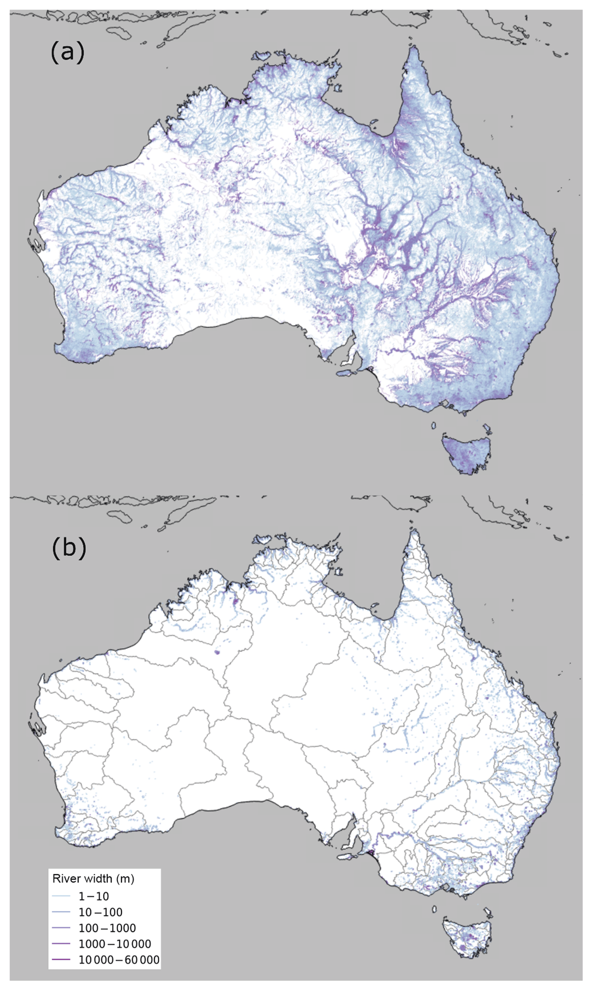
Figure 3Maximum (a) and minimum (b) river width across Australia; 218 river regions delineated in grey in (b).
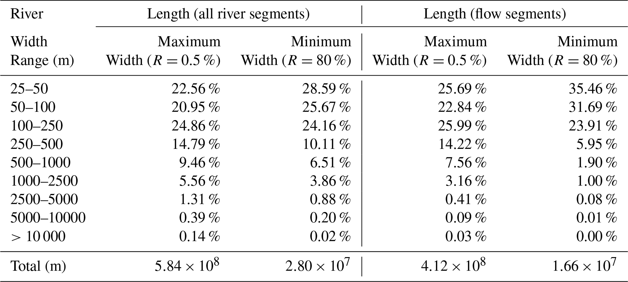
We divided river reaches into three categories based on their maximum width: small (<25 m), medium (25–250 m), and large (>250 m). It is noted that small rivers will not be narrower than 25 m along their entire width; a non-zero width is calculated because some of the 25 m pixels along the reach were mapped as inundated at 0.5 % maximum extent. Therefore, we only list summary statistics here for medium and large rivers (Table 3). The total length of reaches in different maximum and minimum width classes is listed in Table 3, showing the same distribution pattern regardless of whether segments flowing through water bodies are included or excluded. The total length decreases as maximum and minimum river width increases from 25 m up to more than 10 km. The total reach length in different width ranges and at different recurrence frequencies (Fig. 4) decreases by a factor of 21 as frequency increases from 0.5 % to 80 %. The majority of river reaches are 25–250 m broad irrespective of frequency range (Fig. 4).
Table 3The length percentages in different width ranges of maximum (a) and minimum (b) river widths for Australia (all river segments include flow segments and segments flowing through water bodies).
We compared river width at different recurrence frequencies with river gradient for all river reaches, as well as with upstream drainage area and cumulative runoff. For comparison with drainage area and runoff, we included only major rivers because the contribution of upstream flow to minor rivers can be uncertain, for example for anabranches and distributaries. Upstream drainage area and total runoff best predicted maximum reach width, with Pearson correlations of 0.52 and 0.43, respectively, while gradient showed the expected negative relationship with maximum river width (Fig. 5). Reflecting the most common method of river width estimation, we fitted Eq. (1) to our data. We excluded river widths with small upstream cumulative runoff (<104.5 m3 or 0.37 m3 s−1) due to the influence of their sparse distribution on the overall relationship. This resulted in a relationship with a coefficient a=13.17 and exponent b=0.49. We found that reach gradient affects a significantly, with decreasing width as gradient increases, but it did not appear to affect b, except perhaps for the highest gradient class (>0.01, Fig. 6).
River width at 50 % frequency (i.e. median width) was compared with river widths considered representative of “average” flows contained in the GRWL. Among the 218 Australian river regions, only 111 regions had any inundated river channel under “average” conditions in the GRWL river width dataset, whereas all 218 river regions contained detected rivers in our analysis results. The Spearman rank correlation between median river width and river widths from the global dataset exceeded 0.6 for 68 % (75) of 111 river regions and exceeded 0.4 for 86 % (95) of them, suggesting that the two datasets show reasonably similar relative width variations (Fig. 7).
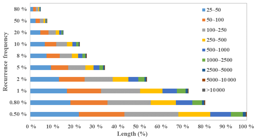
Figure 4The length percentages in different width ranges at different recurrence frequencies for Australia.
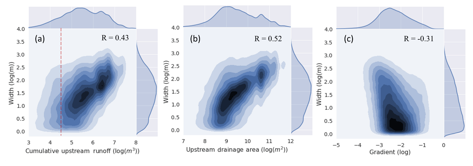
Figure 5The relationships between maximum river width and cumulative upstream runoff (a), upstream drainage area (b), and river gradient (c) (the colour coding is related to data counts with the highest in dark blue and lowest in light blue, which corresponds to the histogram on the axes; red dash line: the threshold (data below this threshold are excluded due to the influence of their sparse distribution on the overall relationship when we fitted Eq. 1 to our data)).
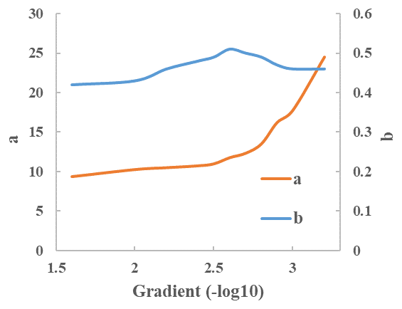
Figure 6The coefficients a and exponents b of the power scaling relationship predicting maximum river width from upstream cumulative runoff (Eq. 1) calculated for different reach gradients.
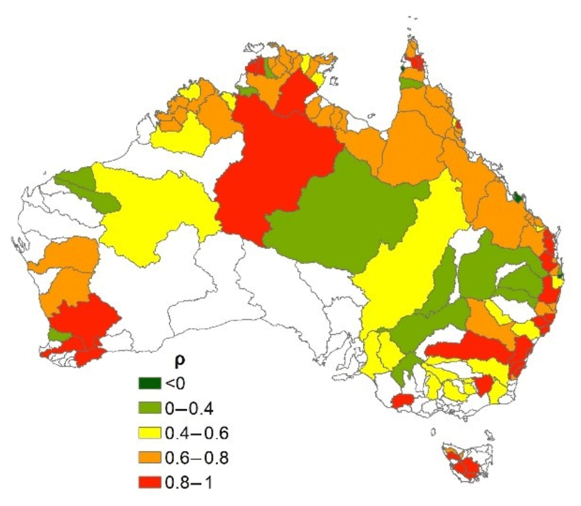
Figure 7The Spearman rank correlations between our dataset and the GRWL dataset in 111 river regions across Australia.
3.2 River hydromorphology classification
The parameter γ represents the degree to which rivers tend towards permanent or ephemeral flow regimes. Most rivers, particularly the larger rivers along the coast, flow through estuaries or other (quasi) permanent water bodies, and hence are classified as permanent or frequent (γ>0.8, Fig. 8). Calculating the combined length of medium and large river reaches in different γ ranges (Fig. 9) shows that the majority fall within γ=0.1–0.6, indicating that the dominant flow regime for Australian rivers is ephemeral or intermittent.
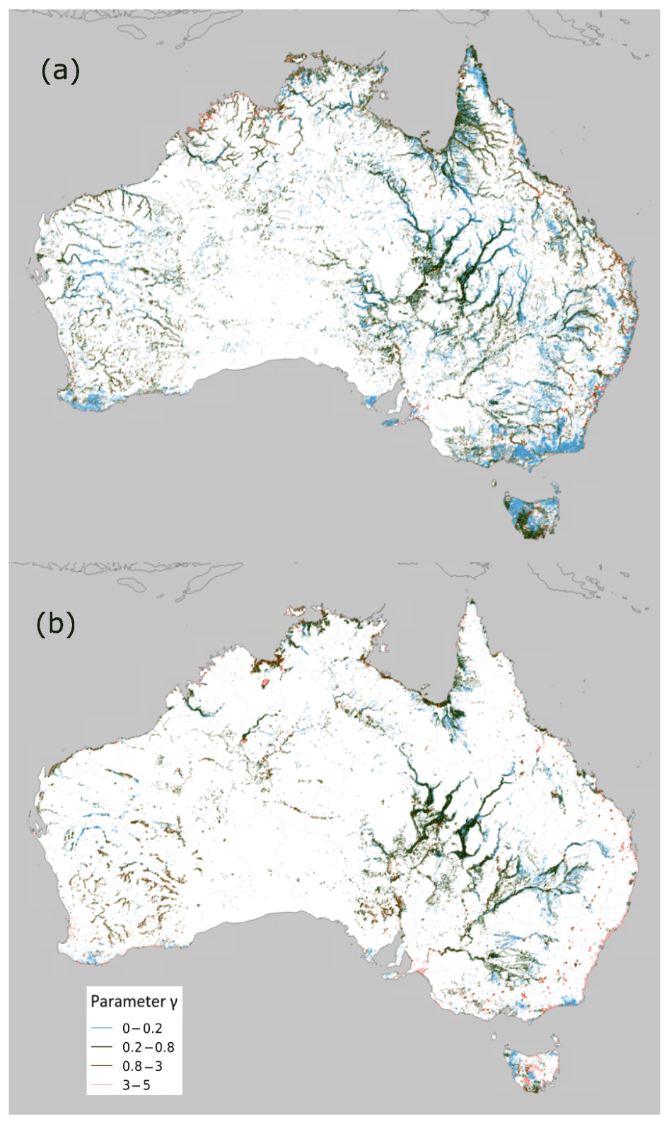
Figure 8River morphology classification γ parameter values for medium (a) and large (b) rivers for Australia.
The average frequency–width data and fitted curves for different γ classes are shown in Fig. 10. The standard differences between observed and fitted width fractions range from 0.0075 to 0.0725 (Table 4). Relative width was overestimated for frequencies between 20 % and 50 % for γ0.6–1.5 and for frequencies between 5 % and 20 % for γ0.2–0.8. Despite these biases, the curves generally capture the relationship between width fraction and frequency well.

Figure 9The length percentages of medium and large rivers for different γ value ranges across Australia.

Figure 10Curve characteristics for different river morphology categories (line: prediction; dot: observation).
3.3 Qualitative evaluation
A longitudinal profile of river width, gradient, and flow regime parameter γ for the main channel of the Murray River (Fig. 11) illustrates several features in the data. Strong width variations between 0.5 % and 80 % frequency can occur, indicating that the river channel contains water for most of the time (>50 % frequency) but contained within a relatively narrow channel. River width increases significantly between 5 %–8 % and 1 %–2 % frequency, which coincides with the threshold for overbank flows. The greatest widths are in reaches flowing through large water bodies, such as Lake Hume (C; storage reservoir), Yarrawonga Weir (D; impoundment), Lake Alexandrina (K; the terminal lake system), and other wetlands (H and I). Where river flows are confined, widths do not change much (e.g. G; Mildura). Where flow splits into multiple channels before converging again, minimum channel width reduces (e.g. E and F), whereas maximum width increases, corresponding to a broader floodplain. Between A and B, river reaches have water for 5 %–8 % of the time in our data, but not in the GRWL dataset (Allen and Pavelsky, 2018) (Fig. 11b). The GRWL widths under “average” conditions are contained within the distribution in our data, but for rather widely varying frequencies. A narrowing relative difference between the 0.5 % and 80 % frequency widths corresponds to higher γ values and vice versa (Fig. 11b). This shows that the river morphology parameter γ can capture the river flow regime. In line with Fig. 5c, river width increases as gradient decreases from upstream to downstream overall (Fig. 11b and c).
Figure 12 illustrates some of the data characteristics and challenges in complex river systems common in Australia's dry and low-relief environments. During floods, all river channels are inundated and rivers are broad (Fig. 12a). Only the main Darling River channel contains water frequently (Fig. 12b), but is still very narrow during low flows (Fig. 12c). All reaches have an ephemeral or intermittent flow regime (Fig. 12f) with γ<0.8, with the southern Talyawalka Creek showing a more ephemeral regime than the Darling River.
Table 4Validation of curves fitting for different river morphology categories.

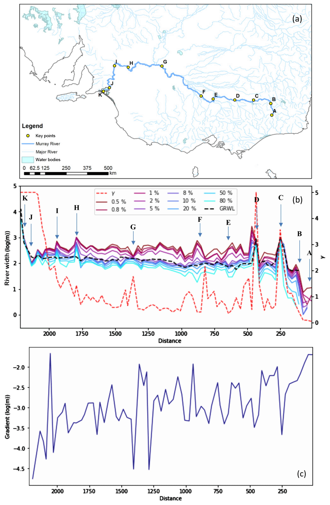
Figure 11Longitudinal profile of the Murray River showing (a) location of river and selected locations; (b) profile of width at different frequencies and river morphology parameter γ; and (c) profile of river gradient. Values are averaged for 30 km sections along the river channel. Letters indicate (A) source according to our data; (B) source according to GRWL data (Allen and Pavelsky, 2018); (C) Lake Hume; (D) Yarrawonga Weir; (E–F) anabranching locations; (G) Mildura; (H–I) Lower Murray wetlands; and (J–K) Lake Alexandrina.
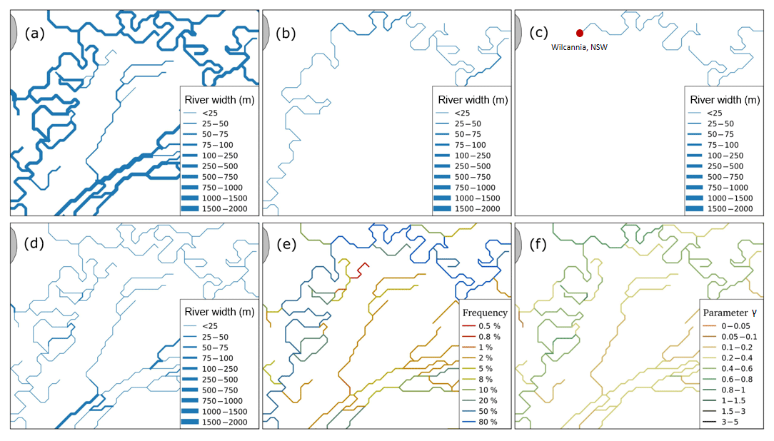
Figure 12Illustration of data characteristics for an area including the Darling River and adjoining Talyawalka Creek near Wilcannia (NSW) (15.7 by 15.3 km centred on 31.62∘ S, 143.42∘ E). Shown are (a) maximum river width (0.5 % frequency); (b) median width (50 %); (c) minimum river width (80 %); (d) least detected river width and (e) corresponding frequency; and (f) hydromorphology parameter γ.
The Geofabric contains nearly 1.4 million river segments across the Australian continent and provides valuable information on river path, length, and contributing sub-catchment area. We were able to assign summary metrics derived from spatial and temporal surface water extent information contained in the satellite-derived WOfS to the river reaches and calculate river widths at different recurrence frequencies. The Geofabric Surface Network had a total length of 3.3 million km. Compared to HydroSHEDS (Lehner et al., 2008), probably the most commonly used global hydrological dataset, the Geofabric delineates a finer-resolution stream network and describes the natural variation in drainage density and complex distributary and anabranching drainage patterns better (Stein et al., 2014). Nonetheless, the 9 s DEM resolution is still insufficient to delineate all floodplains and river flow paths accurately. A new version of the Geofabric at 1 s resolution has been produced for part of Australia, and once available nationally could be used to improve derived river characteristics. Similarly, the WOfS data will continue to receive updates.
Errors in the calculated river characteristics also derive from uncertainties in WOfS inundation mapping. Narrow rivers, small water bodies, and wetlands with vegetation cover may be missed in mapping, and conversely topographical shadows in steep terrain or in high-rise cityscapes can be misclassified as water. Noise in very clear water can also result in misclassification (Mueller et al., 2016). There are also data gaps in WOfS and occasional linear artefacts caused by the Scan-Line-Corrector-Off (SLC-Off) problem in Landsat-7 (Mueller et al., 2016). Nevertheless, the overall accuracy of the water classifier used in WOfS was 97 %, which gives confidence in our derived metrics.
Our dataset has some advantages over existing datasets such as GRWL. Firstly, it provides spatial and temporal information on river dynamics at both in-channel and overbank flows. Secondly, if one river reach has multiple channels, we calculated river width for each channel rather than considering them a single channel. Thirdly, our data provide more detailed information due to the finer river network contained in the Geofabric. Finally, our product can readily be related to any hydrological feature in the Geofabric for further application.
The relationship between river width and contributing catchment area, cumulative runoff, and reach gradient can be compared to literature values. The positive relationships of discharge–width and catchment area–width, and negative relationship of width–gradient have also been demonstrated by Frasson et al. (2019). Empirically relating drainage area to river width (i.e. Eq. 2), Coe et al. (2008) obtained a coefficient c=0.42 and exponent d=0.59, whereas Paiva et al. (2013) found c of 0.35–3.75 and d of 0.36–0.63 for different river basins (Table 5). We found intermediate values of c=0.91 and d=0.43. A more common way to estimate river width is from mean annual discharge (i.e. Eq. 1). Decharme et al. (2008), Getirana et al. (2012, 2013), and Andreadis et al. (2013) all assumed an exponent b=0.5, as suggested by Leopold and Maddock (1953) and Leopold et al. (1964) (Table 5). We found very similar values for the exponent. By contrast, the value of the coefficient a varies widely between studies (Table 5). Getirana et al. (2012, 2013) used a high value of a=18 for the Amazon basin, whereas Andreadis et al. (2013) used a=7.2 for their global application. We estimated a=13.1 for all Australian reaches combined, but also found evidence that a correlates with the river reach gradient (Fig. 6), which may help explain differences between previous studies.
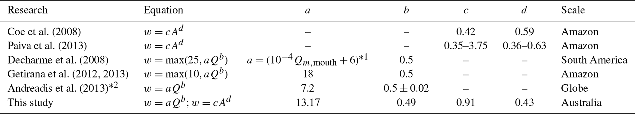
1 Suggested by Arora and Boer (1999) (Qm,mouth is the mean annual discharge at the mouth of the river). 2 Based on the regression relation developed by Moody and Troutman (2002).
Although the empirical scaling functions discussed here can be used to estimate river width based on drainage area or modelled runoff with modest skill, there are also clear limitations. Firstly, they are not able to estimate river widths at different recurrence frequencies. Secondly, individual river reach with the same upstream drainage area or cumulative runoff can have widely different river widths. For example, as mentioned, we found evidence that a reach with a more gentle gradient can be expected to be wider in comparison (Fig. 6), consistent with the Manning equation. Thirdly, scaling equations cannot be applied to multi-channel rivers. Therefore, rather than empirical functions, the river width–frequency relationships derived here should help to improve the description of river morphology in hydrological modelling.
Some uncertainties are inherent to the approach followed here and would benefit from further research. Firstly, we calculated river width based on inundation extent within the entire designated sub-catchment boundary for each river reach. Although this excluded most unrelated water bodies and other river channels, the water mapping may still include unconnected water bodies, such as off-channel storages. This would cause overestimation of river width. However, for analysing width dynamics, normally unconnected water bodies remaining in the sub-catchment can be assumed to be part of the river channel conceptually, because they generally merge with channels at low recurrence frequencies (i.e. high flows) and separate at high recurrence frequencies (i.e. low flows). If these nearby water bodies are removed, it could fail to detect the maximum river width; if they are retained at high flows and removed at low flows, there would be abrupt changes in river width. Secondly, although the data provide detailed information on the width of individual channels in anabranching river systems, the multiple channels will often merge into a single channel during overbank flow events. Our data do not reflect this merging and separating of channels at different flow levels, and it is challenging to find a way to conceptually address this in the Geofabric framework.
Besides, there are some uncertainties from input variables, including DEM, runoff, and length. The SRTM-derived 1 s (approximately 30 m) DEM has a root mean square (rms) error of 3.868 m, and its uncertainties include residual stripes, broad-scale stripes, steps in elevation, large offsets along the edge of the valley floor, noise due to the nature of the radar acquisition and processing, incomplete removal of vegetation offsets and urban and built infrastructure, and vegetation height overestimated (Gallant et al., 2011). However, the majority of rivers flow on flat plains without vegetation cover, and urban and built infrastructure and river gradients were only produced for the main river reaches, presumably with wider channels, which reduce the influence from uncertainties and limitations of DEM. Uncertainties from input data, parameterization, and conceptual structure in the model could affect runoff estimates, although the AWRA-L model has a strong documented pedigree in runoff estimation in comparisons with gauge data (e.g. Van Dijk and Warren, 2010; Frost et al., 2018). The raster–vector conversion anomalies to produce the Geofabric lead to overestimation of the segment length, which to some extent may counterbalance the overestimation of river width.
Looking beyond Australia, the method proposed here is applicable in any region of the world where high-resolution inundation time series mapping is feasible, and where good-quality DEM-derived river path, length, and sub-catchment area data are available. Thus, it would seem feasible to use a similar methodology to that employed here to develop a global river hydromorphology dataset using global inundation time series Landsat mapping produced by Donchyts et al. (2016), Pekel et al. (2016), or Jones (2019), for example.
The river hydromorphology data are available at https://doi.org/10.25914/5c637a7449353 (Hou et al., 2019) and also can be downloaded directly from http://wald.anu.edu.au/data/ (last access: 20 May 2019; ANU Centre for Water and Landscape Dynamics, 2019). The data are in ASCII format, which can be directly joined to the Geofabric products, including surface cartography, surface catchments, surface network, groundwater cartography, and hydrological reporting catchments and regions. The Geofabric Surface Network can be accessed from http://www.bom.gov.au/water/geofabric/ (last access: 20 May 2019; Bureau of Meteorology, 2012b). The instruction for using these data can be found in the “readme” file. The data may be converted to any format (e.g. shapefile or raster) and combined with other Geofabric data, such as river name, length, feature type (nature, artificial, or water area flow segment), hierarchy (major or minor rivers), flow direction, and upstream drainage area.
We developed a river hydromorphology dataset for Australia by combining surface water recurrence information from the WOfS Landsat-derived dynamic water mapping product and GIS-based hydrological features from the Australian Geofabric. Our data provide river widths at different recurrence frequencies for 5.84×10⁸ m river reaches across the Australian continent. A river morphology parameter γ is proposed to describe the shape of the width–frequency curve and can be interpreted as the degree to which rivers tend towards permanent, frequent, intermittent, or ephemeral. The majority of medium and large rivers in Australia have widths between 25 and 250 m and show an ephemeral or intermittent flow regime. The data show correlation between maximum river width and cumulative upstream runoff, upstream drainage area, and gradient, in line with previously published results. The hydromorphological dataset developed contains river width dynamics, flow regime, and river gradient information for all Australian river reaches. The data provide new opportunities to analyse floodplain–river interactions at different scales and analyse the influence of climate, hydrology, vegetation, and terrain on river morphology. Such an understanding can help to predict future changes in landscape evolution in response to e.g. climate change. The dataset developed here may also be useful in providing fundamental information for understanding hydrological, biogeochemical, and ecological processes in floodplain–river systems; describing river width features in hydrological modelling; estimating river depth and discharge; assessing river conveyance capacity; identifying flooding-prone areas, and determining potential locations for satellite-based river gauging (Hou et al., 2018).
JH and AIJMVD conceived the idea. AIJMVD, LJR, RAV, and NM guided the study. JH carried out the research and wrote the manuscript with contributions from all the co-authors.
The authors declare that they have no conflict of interest.
This article is part of the special issue “Linking landscape organisation and hydrological functioning: from hypotheses and observations to concepts, models and understanding (HESS/ESSD inter-journal SI)”. It is not associated with a conference.
The authors acknowledge the Australian Bureau of Meteorology and Geoscience Australia for developing the Australian Hydrological Geospatial Fabric (Geofabric) and Water Observations from Space (WOfS). We are grateful to Adam Lewis for his assistance in reviewing this paper. The first author thanks the ANU-CSC (the Australian National University and the China Scholarship Council) Scholarship for supporting his PhD study at the Australian National University. Calculations were performed on the high-performance computing system, Raijin, from the National Computational Infrastructure (NCI), which is supported by the Australian Government. This paper is published with the permission of the CEO, Geoscience Australia. We also thank Loes van Schaik, George Allen, and the anonymous reviewer for their helpful suggestions that improved the manuscript.
This paper was edited by Loes van Schaik and reviewed by George Allen and one anonymous referee.
Allen, G. H. and Pavelsky, T. M.: Patterns of river width and surface area revealed by the satellite-derived North American river width data set, Geophys. Res. Lett., 42, 395–402, https://doi.org/10.1002/2014GL062764, 2015.
Allen, G. H. and Pavelsky, T. M.: Global extent of rivers and streams, Science, 361, 585–588, https://doi.org/10.1126/science.aat0636, 2018.
Andreadis, K. M., Schumann, G. J. P., and Pavelsky, T.: A simple global river bankfull width and depth database, Water Resour. Res., 49, 7164–7168, https://doi.org/10.1002/wrcr.20440, 2013.
ANU Centre for Water and Landscape Dynamics, available at: http://wald.anu.edu.au/, last access: 20 May 2019.
Arora, V. K. and Boer, G. J.: A variable velocity flow routing algorithm for GCMs, J. Geophys. Res.-Atmos., 104, 30965–30979, https://doi.org/10.1029/1999JD900905, 1999.
Bates, P. D. and De Roo, A. P. J.: A simple raster-based model for flood inundation simulation, J. Hydrol., 236, 54–77, https://doi.org/10.1016/S0022-1694(00)00278-X, 2000.
Biancamaria, S., Bates, P. D., Boone, A., and Mognard, N. M.: Large-scale coupled hydrologic and hydraulic modelling of the Ob river in Siberia, J. Hydrol., 379, 136–150, https://doi.org/10.1016/j.jhydrol.2009.09.054, 2009.
Bureau of Meteorology: Australian Hydrological Geospatial Fabric (Geofabric) Product Guide, available at: http://www.bom.gov.au/water/geofabric/documents/v2_1/ahgf_productguide_V2_1_release.pdf (last access: 20 May 2019), 2012a.
Bureau of Meteorology: Australian Hydrological Geospatial Fabric (Geofabric) Data Product Specification, available at: http://www.bom.gov.au/water/geofabric/documents/v2_1/ahgf_dps_surface_network_V2_1_release.pdf (last access: 20 May 2019), 2012b.
Coe, M. T., Costa, M. H., and Howard, E. A.: Simulating the surface waters of the Amazon River basin: impacts of new river geomorphic and flow parameterizations, Hydrol. Process., 22, 2542–2553, https://doi.org/10.1002/hyp.6850, 2008.
Dadson, S. J., Ashpole, I., Harris, P., Davies, H. N., Clark, D. B., Blyth, E., and Taylor, C. M.: Wetland inundation dynamics in a model of land surface climate: Evaluation in the Niger inland delta region, J. Geophys. Res.-Atmos., 115, D23114, https://doi.org/10.1029/2010JD014474, 2010.
Decharme, B., Douville, H., Prigent, C., Papa, F., and Aires, F.: A new river flooding scheme for global climate applications: Off-line evaluation over South America, J. Geophys. Res.-Atmos., 113, D11110, https://doi.org/10.1029/2007JD009376, 2008.
Doble, R., Crosbie, R., Peeters, L., Joehnk, K., and Ticehurst, C.: Modelling overbank flood recharge at a continental scale, Hydrol. Earth Syst. Sci., 18, 1273–1288, https://doi.org/10.5194/hess-18-1273-2014, 2014.
Donchyts, G., Baart, F., Winsemius, H., Gorelick, N., Kwadijk, J., and Van De Giesen, N.: Earth's surface water change over the past 30 years, Nat. Clim. Change, 6, 810–813, https://doi.org/10.1038/nclimate3111, 2016.
Frasson, R. P. D. M., Pavelsky, T. M., Fonstad, M. A., Durand, M. T., Allen, G. H., Schumann, G., Lion, C., Beighley, R. E., and Yang, X.: Global relationships betwee river width, slope, catchment area, meander wavelength, sinuosity, and discharge, Geophys. Res. Lett., 46, 3252–3262, https://doi.org/10.1029/2019GL082027, 2019.
Frost, A. J., Ramchurn, A., and Smith, A.: The Australian Landscape Water Balance model (AWRA-L v6), Technical Description of the Australian Water Resources Assessment Landscape model version 6, Bureau of Meteorology Technical Report, available at: http://www.bom.gov.au/water/landscape/assets/static/publications/AWRALv6_Model_Description_Report.pdf (last access: 20 May 2019), 2018.
Gallant, J. C., Dowling, T. I., Read, A. M., Wilson, N., Tickle, P., and Inskeep, C.: 1 second SRTM Derived Digital Elevation Models User Guide, Geoscience Australia, available at: https://d28rz98at9flks.cloudfront.net/72759/1secSRTM_Derived_DEMs_UserGuide_v1.0.4.pdf (last access: 20 May 2019), 2011.
Getirana, A. C. V., Boone, A., Yamazaki, D., Decharme, B., Papa, F., and Mognard, N.: The hydrological modeling and analysis platform (HyMAP): Evaluation in the Amazon basin, J. Hydrometeorol., 13, 1641–1665, https://doi.org/10.1175/JHM-D-12-021.1, 2012.
Getirana, A. C. V., Boone, A., Yamazaki, D., and Mognard, N.: Automatic parameterization of a flow routing scheme driven by radar altimetry data: Evaluation in the Amazon basin, Water Resour. Res., 49, 614–629, https://doi.org/10.1002/wrcr.20077, 2013.
Hou, J., Van Dijk, A. I. J. M., Renzullo, L. J., and Vertessy, R. A.: Using modelled discharge to develop satellite-based river gauging: a case study for the Amazon Basin, Hydrol. Earth Syst. Sci., 22, 6435–6448, https://doi.org/10.5194/hess-22-6435-2018, 2018.
Hou, J., Van Dijk, A. I. J. M., Renzullo, L. J., Vertessy, R. A., and Mueller, N.: Hydromorphological attributes for all Australian river reaches, Dataset, https://doi.org/10.25914/5c637a7449353, 2019.
Isikdogan, F., Bovik, A., and Passalacqua, P.: RivaMap: An automated river analysis and mapping engine, Remote Sens. Environ., 202, 88–97, https://doi.org/10.1016/j.rse.2017.03.044, 2017.
Jones, J. W.: Improved Automated Detection of Subpixel-Scale Inundation – Revised Dynamic Surface Water Extent (DSWE) Partial Surface Water Tests, Remote Sens., 11, 374, https://doi.org/10.3390/rs11040374, 2019.
Kleinhans, M. G. and Van Den Berg, J. H.: River channel and bar patterns explained and predicted by an empirical and a physics-based method, Earth Surf. Process. Landf., 36, 721–738, https://doi.org/10.1002/esp.2090, 2011.
Lehner, B., Verdin, K., and Jarvis, A.: New global hydrography derived from spaceborne elevation data, Eos, Trans. Am. Geophys. Union, 89, 93–94, https://doi.org/10.1029/2008EO100001, 2008.
Leopold, L. B. and Maddock, T.: The hydraulic geometry of stream channels and some physiographic implications, U.S. Government Printing Office, Washington, D.C., 1953.
Leopold, L. B., Wolman, M. G., and Miller, J. P.: Fluvial processes in geomorphology, W.H. Freeman and Company, San Francisco, 1964.
Miller, Z. F., Pavelsky, T. M., and Allen, G. H.: Quantifying river form variations in the Mississippi Basin using remotely sensed imagery, Hydrol. Earth Syst. Sci., 18, 4883–4895, https://doi.org/10.5194/hess-18-4883-2014, 2014.
Moody, J. A. and Troutman, B. M.: Characterization of the spatial variability of channel morphology, Earth Surf. Process. Landf., 27, 1251–1266, https://doi.org/10.1002/esp.403, 2002.
Mueller, N., Lewis, A., Roberts, D., Ring, S., Melrose, R., Sixsmith, J., Lymburner, L., McIntyre, A., Tan, P., Curnow, S., and Ip, A.: Water observations from space: Mapping surface water from 25 years of Landsat imagery across Australia, Remote Sens. Environ., 174, 341–352, https://doi.org/10.1016/j.rse.2015.11.003, 2016.
Nanson, G. C. and Knighton, A. D.: Anabranching rivers: their cause, character and classification, Earth Surf. Process. Landf., 21, 217–239, https://doi.org/10.1002/(SICI)1096-9837(199603)21:3<217::AID-ESP611>3.0.CO;2-U, 1996.
Neal, J., Schumann, G., and Bates, P.: A subgrid channel model for simulating river hydraulics and floodplain inundation over large and data sparse areas, Water Resour. Res., 48, W11506, https://doi.org/10.1029/2012WR012514, 2012.
NIST/SEMATECH e-handbook of statistical methods, available at: http://www.itl.nist.gov/div898/handbook (last access: 20 May 2019), 2018.
O'Loughlin, F., Trigg, M. A., Schumann, G. J. P., and Bates, P. D.: Hydraulic characterization of the middle reach of the Congo River, Water Resour. Res., 49, 5059–5070, https://doi.org/10.1002/wrcr.20398, 2013.
Paiva, R. C. D., Buarque, D. C., Collischonn, W., Bonnet, M. P., Frappart, F., Calmant, S., and Mendes, C. A. B.: Large-scale hydrologic and hydrodynamic modeling of the Amazon River basin, Water Resour. Res., 49, 1226–1243, https://doi.org/10.1002/wrcr.20067, 2013.
Pavelsky, T. M. and Smith, L. C.: RivWidth: A software tool for the calculation of river widths from remotely sensed imagery, IEEE Geosci. Remote Sens. Lett., 5, 70–73, https://doi.org/10.1109/LGRS.2007.908305, 2008.
Pedinotti, V., Boone, A., Decharme, B., Crétaux, J. F., Mognard, N., Panthou, G., Papa, F., and Tanimoun, B. A.: Evaluation of the ISBA-TRIP continental hydrologic system over the Niger basin using in situ and satellite derived datasets, Hydrol. Earth Syst. Sci., 16, 1745–1773, https://doi.org/10.5194/hess-16-1745-2012, 2012.
Pekel, J.-F., Cottam, A., Gorelick, N., and Belward, A. S.: High-resolution mapping of global surface water and its long-term changes, Nature, 540, 418–422, https://doi.org/10.1038/nature20584, 2016.
Rosgen, D. L.: A classification of natural rivers, Catena, 22, 169–199, https://doi.org/10.1016/0341-8162(94)90001-9, 1994.
Stein, J. L., Hutchinson, M. F., and Stein, J. A.: A new stream and nested catchment framework for Australia, Hydrol. Earth Syst. Sci., 18, 1917–1933, https://doi.org/10.5194/hess-18-1917-2014, 2014.
Storn, R. and Price, K.: Differential evolution–a simple and efficient heuristic for global optimization over continuous spaces, J. Global Optim., 11, 341–359, https://doi.org/10.1023/A:1008202821328, 1997.
Van Dijk, A. I. J. M.: Australian Water Resources Assessment System. Technical Report 3. Landscape Model (version 0.5) Technical Description. CSIRO: Water for a Healthy Country. National Research Flagship, available at: http://www.clw.csiro.au/publications/waterforahealthycountry/2010/wfhc-aus-water-resources-assessment-system.pdf (last access: 20 May 2019), 2010.
Van Dijk, A. I. J. M. and Warren, G.: The Australian Water Resources Assessment System. Technical Report 4, Landscape Model (version 0.5) Evaluation Against Observations, CSIRO: Water for a Healthy Country National Research Flagship, available at: http://www.clw.csiro.au/publications/waterforahealthycountry/2010/wfhc-awras-evaluation-against-observations.pdf (last access: 20 May 2019), 2010.
Van Schaik, L., Hohenbrink, T., Jackisch, C., Laudon, H., Pfister, L., Hassler, S. K., Renner, M., and Gelfan, A. (Eds.): Linking landscape organisation and hydrological functioning: from hypotheses and observations to concepts, models and understanding, special issue jointly organized between Hydrology and Earth System Sciences and Earth System Science Data, https://www.earth-syst-sci-data.net/special_issue13_985.html, 2019.
Vincenty, T.: Direct and inverse solutions of geodesics on the ellipsoid with application of nested equations, Surv. Rev., 23, 88–93, https://doi.org/10.1179/sre.1975.23.176.88, 1975.
Yamazaki, D., Kanae, S., Kim, H., and Oki, T.: A physically based description of floodplain inundation dynamics in a global river routing model, Water Resour. Res., 47, W04501, https://doi.org/10.1029/2010WR009726, 2011.
Yamazaki, D., O'Loughlin, F., Trigg, M. A., Miller, Z. F., Pavelsky, T. M., and Bates, P. D.: Development of the global width database for large rivers, Water Resour. Res., 50, 3467–3480, https://doi.org/10.1002/2013WR014664, 2014.