Historical gridded reconstruction of potential evapotranspiration for the UK

Potential evapotranspiration (PET) is a necessary input data for most hydrological models and is often needed at a daily time step. An accurate estimation of PET requires many input climate variables which are, in most cases, not available prior to the 1960s for the UK, nor indeed most parts of the world. Therefore, when applying hydrological models to earlier periods, modellers have to rely on PET estimations derived from simplified methods. Given that only monthly observed temperature data is readily available for the late 19th and early 20th century at a national scale for the UK, the objective of this work was to derive the best possible UK-wide gridded PET dataset from the limited data available.

To that end, firstly, a combination of (i) seven temperature-based PET equations, (ii) four different calibration approaches and (iii) seven input temperature data were evaluated. For this evaluation, a gridded daily PET product based on the physically based Penman–Monteith equation (the CHESS PET dataset) was used, the rationale being that this provides a reliable “ground truth” PET dataset for evaluation purposes, given that no directly observed, distributed PET datasets exist. The performance of the models was also compared to a “naïve method”, which is defined as the simplest possible estimation of PET in the absence of any available climate data. The “naïve method” used in this study is the CHESS PET daily long-term average (the period from 1961 to 1990 was chosen), or CHESS-PET daily climatology.

The analysis revealed that the type of calibration and the input temperature dataset had only a minor effect on the accuracy of the PET estimations at catchment scale. From the seven equations tested, only the calibrated version of the McGuinness–Bordne equation was able to outperform the “naïve method” and was therefore used to derive the gridded, reconstructed dataset. The equation was calibrated using 43 catchments across Great Britain.

The dataset produced is a 5 km gridded PET dataset for the period 1891 to 2015, using the Met Office 5 km monthly gridded temperature data available for that time period as input data for the PET equation. The dataset includes daily and monthly PET grids and is complemented with a suite of mapped performance metrics to help users assess the quality of the data spatially.

This dataset is expected to be particularly valuable as input to hydrological models for any catchment in the UK.

The data can be accessed at https://doi.org/10.5285/17b9c4f7-1c30-4b6f-b2fe-f7780159939c.

1 Introduction

Potential evapotranspiration is a conceptual variable which measures the atmospheric demand for moisture from an open surface water. Reference crop evapotranspiration (also referred to as potential evapotranspiration PET) is the rate of evapotranspiration of an idealised short grass actively growing and not short of water (Shuttleworth, 1993), providing an upper limit of the evaporative losses of grass. As evapotranspiration is a major factor in the catchment water balance (Beven, 2012), PET is used as input data for rainfall–runoff models.

Different approaches have been proposed for estimating PET. The most complex, combination methods, are based on physical processes accounting for the energy available to a plant to evaporate during photosynthesis, and the amount of water that can be dissipated in the atmosphere (Penman, 1948; Monteith, 1965). They are referred to as combination methods as they combine the energy balance with the mass transfer method. The simplest methods aim to capture the dominant climatic factors in the plant evapotranspiration processes. The simplified methods can be broadly divided between the radiation-based methods (e.g. Doorenbos and Pruitt, 1984; Hargreaves and Samani, 1983; Jensen and Haise, 1963), which use measured data such as net solar radiation, sunshine hours or cloudiness factors; and the temperature-based methods (e.g. Blaney and Criddle, 1950; Thornthwaite, 1948; Oudin et al., 2005; McGuinness and Bordne, 1972), which use temperature as a proxy for the radiative energy available, along with extraterrestrial radiation estimated from the date of the year and latitude. Both radiation and temperature methods are used instead of combination methods when the full set of climatic variables necessary for the latter is not readily available. However, there is no general agreement on the best performing method, and the final choice of the equation often depends on the application and data availability, as well as the particular environmental setting (e.g. Donohue et al., 2010; Federer et al., 1996; Oudin et al., 2005; Prudhomme and Williamson, 2013; Xu and Singh, 2000, 2001). When little or no climatic variables are available, an alternative is to use remote-sensing data in simplified empirical PET methods (Barik, 2014; Barik et al., 2016; Knipper, 2017; Mu, 2013), however this can only be applied to the satellite era (from the 1970s or the 1980s).

In the UK, the Met Office Rainfall and Evaporation Calculation System (MORECS) (Thompson et al., 1982) is one of the main sources of PET estimates, available as an approximately 40 × 40 km monthly gridded product, with time series from 1961. MORECS is based on the Penman–Monteith formulation (Monteith, 1965), but includes evaporation from rainfall intercepted by the canopy and considers 14 different vegetation types and three different soils (Hough, 2003). Recently, the Centre for Ecology and Hydrology (CEH) published the Climate, Hydrology and Ecology research Support System (CHESS), a 1 km gridded daily meteorological and land state dataset for Great Britain (Robinson et al., 2016a, b, 2017) spanning the period 1961–2015. It includes PET data calculated from the meteorological variables using the Penman–Monteith equation for a well-watered grass surface, following the Food and Agriculture Organisation of the United Nations (FAO) guidelines for computing reference crop PET (Allen, 1998), both with and without corrections for water intercepted by the canopy (Robinson et al., 2016b).

In the UK, PET data is widely used for hydrological modelling, where streamflow time series are generated from rainfall and PET inputs. This is particularly useful in providing information where streamflow observations do not exist, i.e. in reconstructing flows for pre-observational periods, or to explore the response of a changing climate on hydrology. Currently, there is no readily available source of PET time series for studying long-term variability and change in hydrological regimes before the 1960s, including water resources availability and drought patterns. This is a major obstacle, because historical drought periods are used in water resources and drought planning (Watts et al., 2012), as well as for providing a baseline of past hydrological variability for future change assessments. In practice, however, limited availability of atmospheric variables makes it difficult to account for the majority of evapotranspiration processes for the pre-1960 period using the Penman–Monteith equation. Simpler methods therefore need to be used as an alternative, but this requires a thorough evaluation of the differences they bring when compared with established datasets. This study focuses on temperature-based PET equations as temperature (together with precipitation) are among the climate variables that have observed, spatially distributed records for the longest period for the UK. High-resolution gridded (5 km) temperature and precipitation data from the Met Office are available from 1910, and have recently been extended back in time as part of historical data rescuing effort by the Met Office funded by the Historic Droughts project. Monthly temperature and precipitation data were available to project partners from 1891 and 1862 respectively. Detailed climatic variables are available in the UK only from 1961 onwards. Some other variables such as sea level pressure data are also available from late 19th century (Met Office HADSLP2 product), however the spatial resolution is much coarser (5^∘).

While the focus was on applying PET methods for historical reconstruction, this undertaking will provide useful information for other applications where only temperature data are available; for example, hydrological forecasting or long-term climate change impact studies.

This paper describes the derivation of a 5 km gridded daily and monthly PET dataset for the UK from 1891 to 2015, with hydrological modelling being the main targeted application. First, the data used for calibration, validation and production of the gridded dataset are presented. This is followed by the methods, where the temperature-based PET equations, the calibration strategies and the evaluation approach used are described. Thirdly, the results of the evaluation of the PET equations, and the assessment of the final PET grids are presented. Lastly, uncertainties and limitations of the product are discussed, and recommendations for users are listed.

2 Data

This study has used various gridded temperature and PET datasets, which are described in this section. Table 1 provides a summary of all datasets used.

2.1 Temperature data

Three main sources of high-resolution gridded national-scale temperature data exist for the UK:

• CHESS-met high-resolution mean daily temperature (1 km grids, daily time series) for 1961–2015 for Great Britain (henceforth CHESS-temp daily). This dataset is part of a larger dataset developed by CEH for environment modelling applications; its derivation is fully described in Robinson et al. (2016a).

• UKCP09 mean monthly temperature (5 km grids, monthly time series) for 1910–2015 for the UK, including Northern Ireland (henceforth UKCP09-temp monthly). This is part of a larger dataset developed by UK Met Office, its derivation is fully described in Perry and Hollis (2005). The monthly mean temperature is derived from the average of daily maximum and minimum temperature averaged across the month at each contributing station. Stations with no more than two missing days within a calendar month are used to create the gridded product.

• Historic droughts mean monthly temperature (5 km grids, monthly time series) for 1891–1909 for the UK, including Northern Ireland (henceforth HD-temp monthly). This was derived using the same methodology as UKCP09, using historic weather station data rescued by the Met Office in the Historic Droughts project (NERC grant number: NE/L01016X/1).

The two latter were combined in this study and treated as a single dataset to provide a single, continuous record of temperature from 1891 to 2015, which is used to derive the long-term potential evapotranspiration dataset that is the focus of this study. The combined dataset will be referred to as UKCP09 in the rest of the paper. The uncertainty associated with the temperature dataset is discussed in Sect. 5.1. The shorter (1961–2015) CHESS dataset is used for calibration and sensitivity testing.

Table 1 Summary of temperature and PET datasets used in this study. (a) Temperature data used to investigate the effect of temporal distribution of data on the output PET estimation, (b) temperature data to investigate effect of spatial resolution of the data on the output PET estimation, and (c) PET data used to calibrate and evaluate the equation and final PET output.

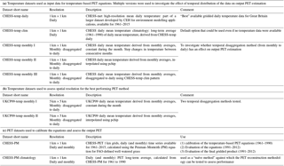
Prior to 1961, temperature data is only available at a 5 km spatial resolution and monthly time step. Because of this coarser temporal and spatial resolution of temperature data in the earlier period, alternative datasets were generated and used in the analysis to quantify the sensitivity of PET derivation to temperature input, and are summarised in Table 1a and b:

• CHESS daily mean temperature climatology (1 km grids) (henceforth CHESS-temp clim): long-term average (1961–1990) of daily mean temperature, derived from CHESS-temp daily. This provides a default option that could be used even if no temperature data were available in the past (or future). This gives a day-to-day variability pattern of temperature throughout the year, which is then repeated every year.

• CHESS daily mean temperature derived from monthly averages (1 km grids). Different methods to disaggregate monthly temperature into daily data were tested:

  • i.

    Constant temperature during the month (henceforth CHESS-temp monthly I). This means there are step changes in temperature between consecutive months.

  • ii.

    Interpolated using pchip method for a smooth transition between months (henceforth CHESS-temp monthly II). Pchip stands for piecewise cubic hermite interpolating polynomial, which is an interpolation method in which a cubic polynomial approximation is assumed over each subinterval. Aràndiga et al. (2016) describe this interpolation scheme in detail together with its advantages, mainly that it is both accurate (preserves values at the nodes) and preserves monotonicity. Pchip was selected for the present study because (i) the fitted curve passes through observed values at inflexion points unlike spline or quadratic methods, for example, and (ii) it does not require re-fitting when the period of application is extended as each subinterval is treated separately.

  • iii.

    Disaggregated to daily using CHESS daily mean temperature climatology pattern (henceforth CHESS-temp monthly III). The daily relative variation in temperature follows the climatology, but for each month, the daily values are adjusted so that monthly mean temperatures are correct. In other words, CHESS-temp clim data is shifted uniformly so the monthly mean temperature matches the CHESS monthly temperature data.

• UKCP09 daily mean temperature (5 km grids) derived from monthly averages. Two different methods to disaggregate monthly temperature into daily data were tested:

  • i.

    Constant during the month (henceforth UKCP09-temp monthly I).

  • ii.

    Interpolated using pchip method (henceforth UKCP09-temp monthly II).

Figure S1 in the Supplement illustrates what these different temperature time series look like for an example catchment. Figure S2 in the Supplement shows the spatial coverage of the different datasets used in this study (Fig. S2a and b), whereas Fig. S2c shows the geographical extend of Great Britain, Northern Ireland and the UK.

In summary, seven different daily temperature datasets were used as input data to the temperature-based PET equations: CHESS-temp daily, CHESS-temp clim, CHESS-temp monthly I, CHESS-temp monthly II, CHESS-temp monthly III, UKCP09-temp monthly I and UKCP09-temp monthly II. CHESS-temp daily is an existing dataset (https://catalogue.ceh.ac.uk/documents/b745e7b1-626c-4ccc-ac27-56582e77b900, last access: 30 April 2018), whereas the other six daily datasets are manipulated versions of existing datasets (CHESS or UKCP09).

2.2 PET

One main source of national-scale mean daily PET time series was available: CHESS-PET 1 km grids, daily time series (Robinson et al., 2016b) available for 1961–2015, calculated using the Penman–Monteith (PM) equation (Monteith, 1965) for FAO-defined well-watered grass (Allen, 1998). Because the PM equation is a physically based model which combines the energy balance with the mass transfer method, and is recommended by the FAO to calculate PET, CHESS-PET daily is here considered as “ground truth” and proxy for observations (hereafter referred to as CHESS-PM).

CHESS-PM daily climatology (hereafter CHESS-PM climatology) was also calculated from 1961 to 1990, and is used as a “naïve method” against which the PET reconstruction methodology can be tested to assess performance. “Naïve method” here refers to the simplest way PET could be estimated in the absence of any climate data.

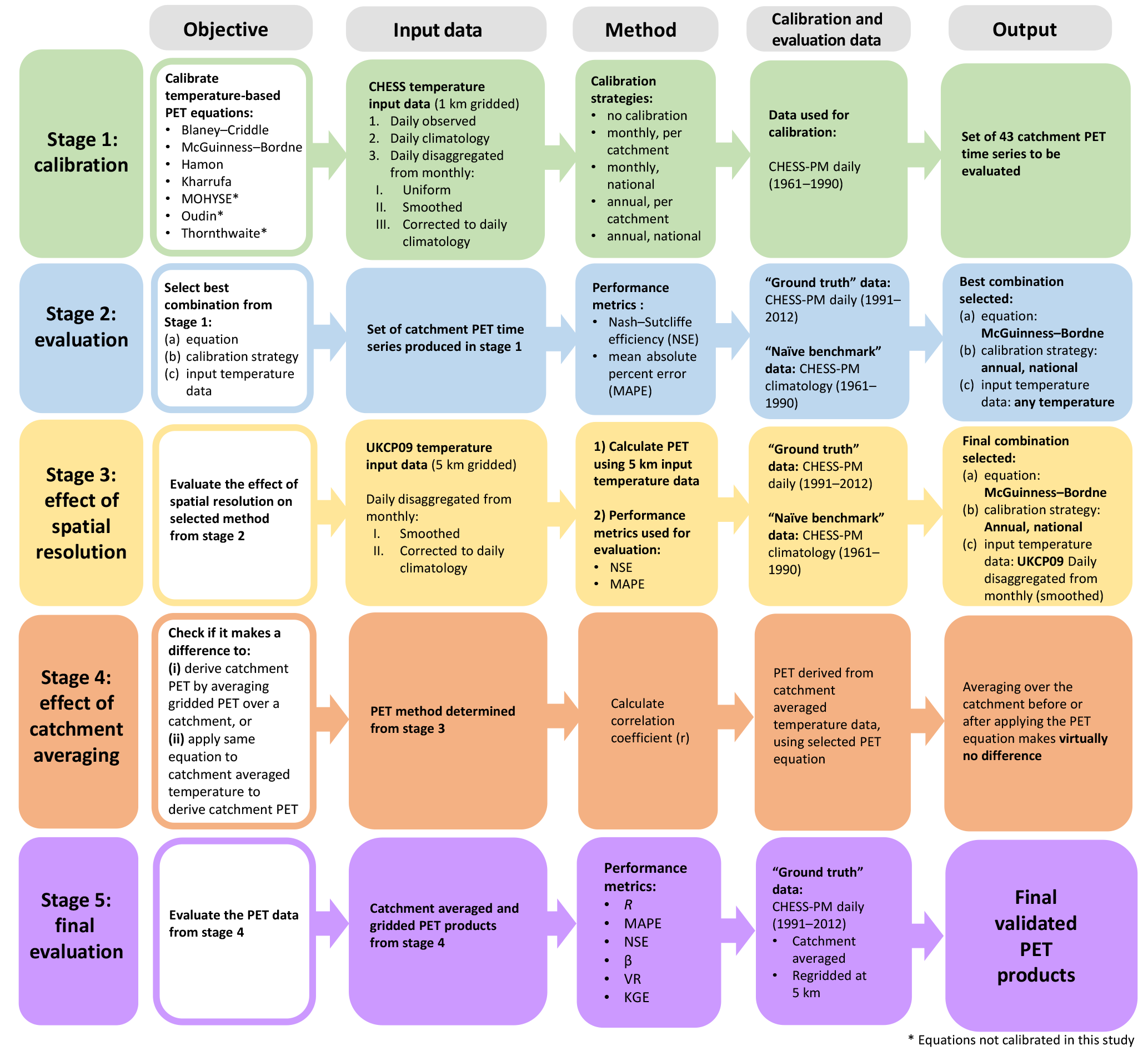
Figure 1 Work flow diagram of the evaluation procedure of the PET equations and final PET gridded product. This process was made in five stages: in stage 1, the equations were calibrated using different calibration strategies and different input temperature data; in stage 2, the multiple combinations of PET equation/calibration approach/temperature input data were evaluated; in stage 3, the effect of spatial resolution of the input temperature data was assessed. These first three stages led to the selection of PET equation, calibration strategy and input dataset used to produce the final gridded PET product. In the fourth stage, the effect of calibrating the equations at the catchment scale was investigated; and finally, in stage 5, a final evaluation of the new gridded PET product was carried out both at the catchment scale and at the grid scale. Stages 1, 2 and 3 used the set of 43 catchments shown in Fig. 2a, whereas stages 4 and 5 used the full set of 306 evaluation catchments shown in Fig. 2b.

Table 2 Temperature-based equations evaluated in this study.

3 Methods

To produce the PET gridded reconstruction product, a sequence of assessments and tests were first undertaken. In the first stage, a set of seven temperature-based equations (presented in Sect. 3.1) were tested with seven different input temperature datasets (Sect. 2.1) and four calibration strategies (Sect. 3.2) (in addition to the non-calibrated equations). These combinations of equation/calibration strategy/temperature input data were evaluated in the second stage (Sect. 3.3.1), leading to the selection of the best combination. In the third stage, the effect of the spatial resolution was investigated (Sect. 3.2.2.), followed by a study of the effect of averaging over the catchments in the fourth stage (Sect. 3.2.2.). Finally, in the fifth stage, the final PET gridded product was evaluated with the calculation of performance metrics both at catchment scale and grid scale (Sect. 3.2.2.). Figure 1 is a workflow diagram summarising the different stages of the work.

3.1 Temperature-based equations

Seven temperature-based equations were evaluated (see Table 2). Four of them (Eqs. 1–4 in Table 2) were calibrated testing different calibration strategies (Sect. 3.2): Hamon (Hamon, 1961), McGuinness–Bordne (McGuinness and Bordne, 1972), Blaney–Criddle (Blaney and Criddle, 1950) and Kharrufa (Kharrufa, 1985). Each contains a number of parameters representative of the climatic region where the equation was originally developed, which can be calibrated to match the climatic regime of the UK. The other three equations were not suitable for simple calibration techniques, or had set calibrations: Oudin (Oudin et al., 2005), MOHYSE (Fortin and Turcotte, 2006) and Thornthwaite (Thornthwaite, 1948) (Eqs. 5 to 7 in Table 2).

The physical basis for estimating evaporation using temperature alone is that both terms of the combination equation (the energy required to sustain evaporation and the energy removed from the surface as water vapour) are generally related to temperature (Shuttleworth, 1993).

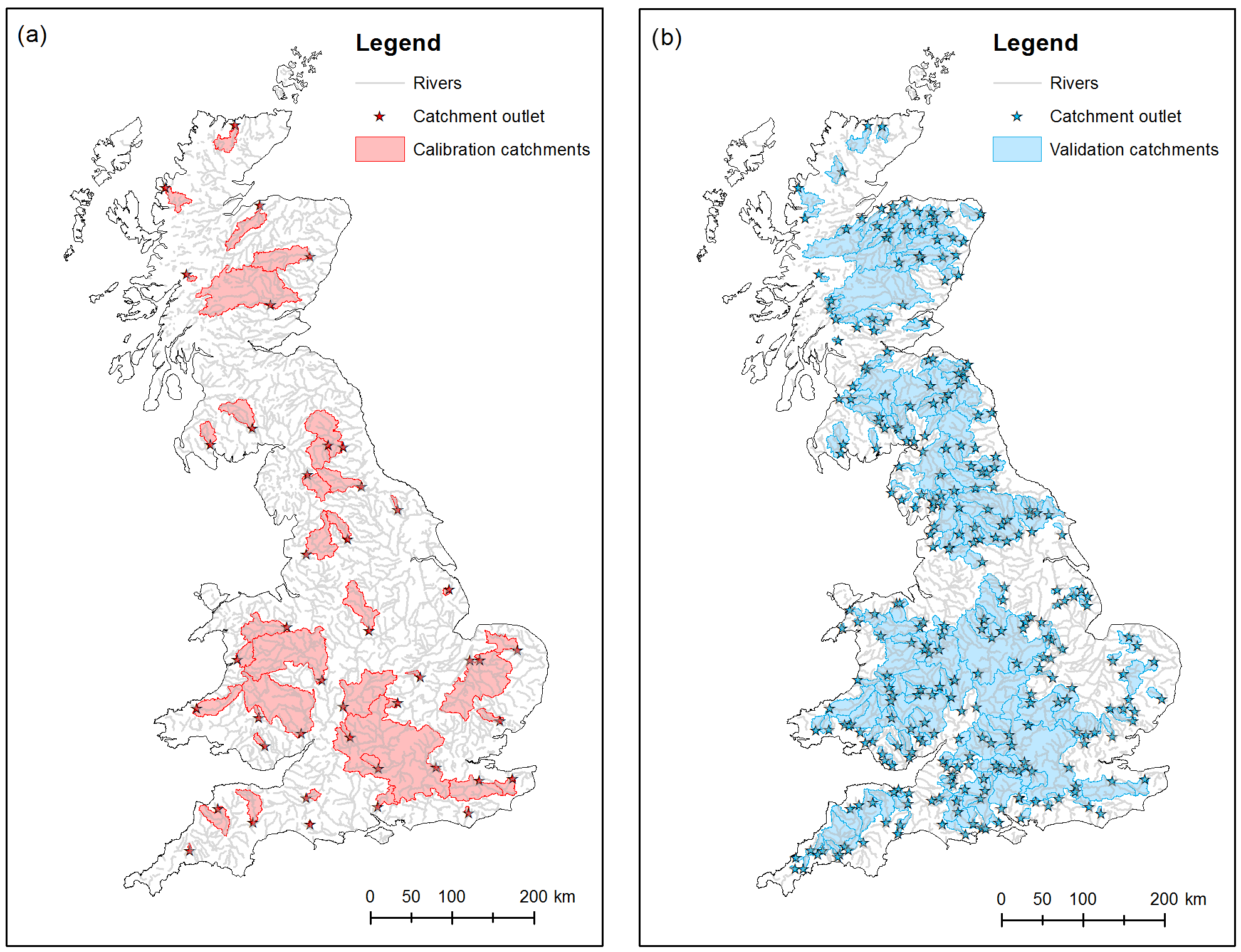
Figure 2 Maps of the boundaries and outlets of (a) catchments that were used to calibrate the PET equations and to calculate the performance metrics of the PET equations, described in Sect. 3.3.1 (stages 1, 2 and 3 in Fig. 1); and (b) catchments that were used to carry out the assessment of the final PET grids using the performance metrics described in Sect. 3.3.2 (stages 4 and 5 in Fig. 1).

The main difference between the different temperature-based formulations, lies in the way temperature is linked to PET to simulate the effect of the full set of variables normally required in the combination equations. Most temperature-based equations use day length or related variables (Hamon, 1961; Blaney and Criddle, 1950; Kharrufa, 1985; Fortin and Turcotte, 2006; Thornthwaite, 1948), except McGuinness and Bordne (1972), and the derived Oudin et al. (2005)'s equation which use extraterrestrial radiation instead. Blaney–Criddle equation has also an additional parameter k, which depends on crop type. Most of these equations were developed for the USA, except MOHYSE (which was developed in Quebec), Kharrufa (developed for arid regions) and Oudin (developed in Australia, USA and France).

Note that equations requiring minimum and maximum temperature (Droogers and Allen, 2002; Hargreaves and Samani, 1983; Heydari and Heydari, 2014) were not considered here as only low-data demanding methods that could be easily reproduced and extended in cases of minimal data availability were selected.

3.2 Calibration strategies

To compare the different calibration methods (stage 1 in Fig. 1), the calibration and testing was done at catchment scale using two independent sets of catchments representative of typical hydroclimatic conditions prevailing in the UK and with good spatial coverage: 43 were used for calibration and assessment of the equations, and an additional 263 (making a total of 306 catchments) used for evaluation of the final PET grids (Fig. 2). Table S1 (Excel spreadsheet) in the Supplement shows the catchments with some of their catchment characteristics. The spatial averaging of temperature and PET time series to conduct the analysis has the advantage of smoothing out any discontinuity that could exist at the grid-scale level due to different interpolation algorithms and recording stations and which could consequently impact on local performance of the PET generation technique. In addition, for many practical hydrological modelling applications, PET is required at the catchment scale. The impact of catchment-scale vs. grid-scale calibration is assessed in Sect. 4.2 (stage 4 in Fig. 1).

As previously mentioned, temperature-based PET equations use parameters to link temperature to PET as a simplification of full evaporation dynamics. Because of important climatic variation across space, and in time across the year, it might be possible that optimal parameterisation could be achieved by letting the parameters vary in time and space. Therefore, four calibration strategies, which are graphically represented in Fig. 3, were considered. The simplest one consists in a global parameterisation (GB) leading to a single equation (1P) for all 43 catchments (1P-GB). In the most complex approach, a local and monthly parametrisation leads to 12 equations for each of the 43 catchments (12P-ind). The trade-off between a simplified method (global parameterisation), which is much easier to implement, and a local method, which requires a long calibration procedure and a parameter transfer methodology for Northern Ireland (where no daily PET dataset is available), is discussed in the results section.

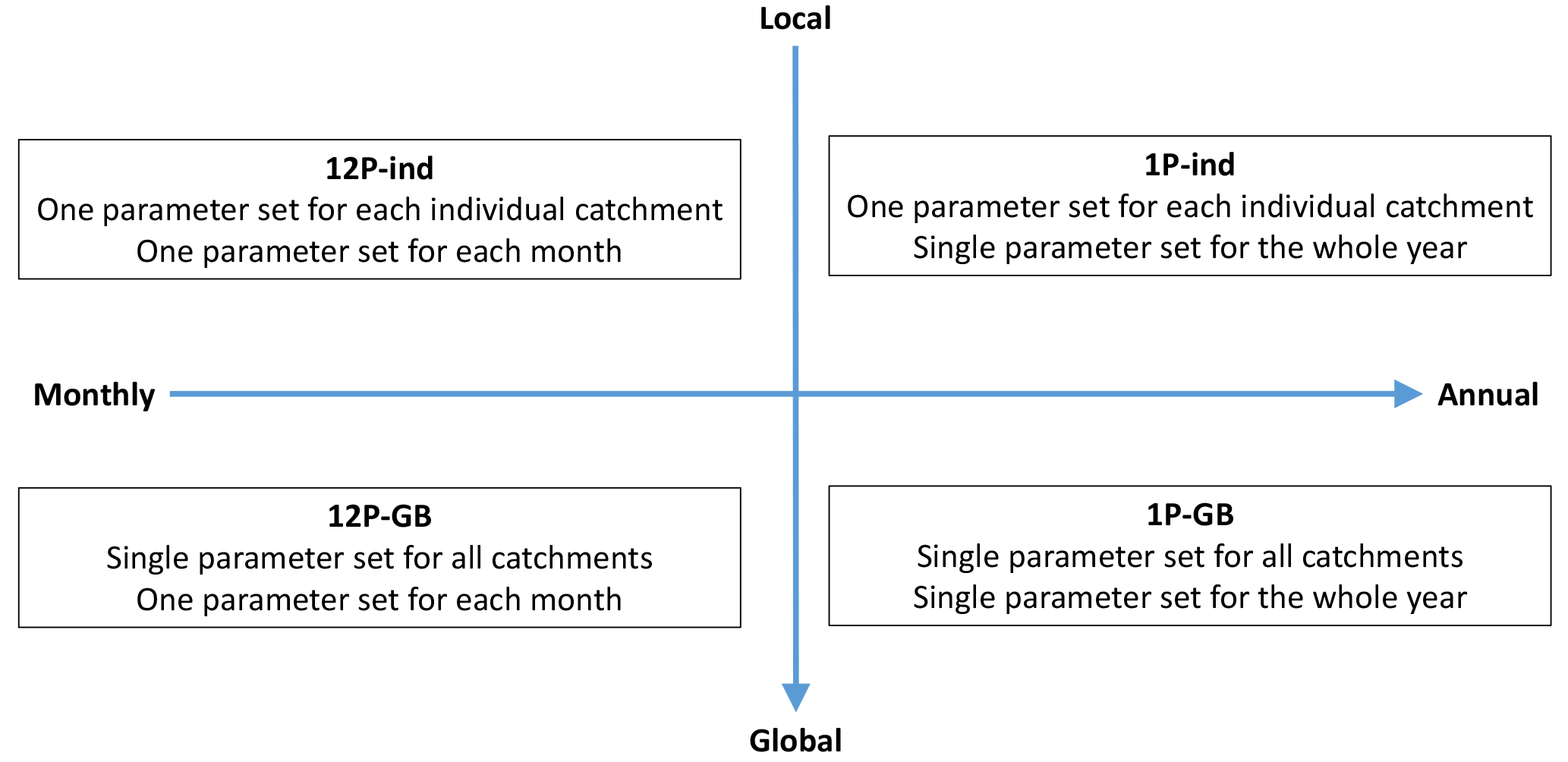
Figure 3 Schematic of the calibration strategies. Four calibration approaches were considered to calibrate the PET equations: from local and monthly parametrisation leading to 12 equations for each of the 43 catchments (12P-ind), to a global parameterisation leading to a single equation for all 43 catchments (1P-GB).

Two independent time periods were selected for the calibration (1961–1990) and evaluation (1991–2012) procedures. The equations' parameters were calibrated using the ordinary least squares (OLS) method against CHESS-PM. The data showed some heteroscedasticity and a moderate degree of autocorrelation, which violates the assumption of OLS. However the effect of these violations has been investigated and does not affect parameter estimations in our particular case. More detail on this can be found in the Supplement (Sect. S1).

3.3 Evaluation

3.3.1 Catchment-scale performance metrics for evaluating the combinations of PET equations/calibration strategy/input temperature data

This evaluation corresponds to stage 2 in Fig. 1, and was done on the 43 calibration catchments shown in Fig. 2a for the period 1991–2012.

Two metrics were used to evaluate the best combination of temperature data, PET equation, and calibration strategy: the mean absolute percentage error (MAPE) and Nash–Sutcliffe efficiency (NSE) coefficient, using CHESS-PM daily as ground truth.

MAPE is widely used in the forecasting community to evaluate accuracy of output from models (Danladi et al., 2017; Lefebvre and Bensalma, 2015). Applied to PET, it is calculated as follows:

$${\displaystyle }\mathrm{MAPE}={\displaystyle \frac{\mathrm{100}}{n}}\sum _{t=\mathrm{1}}^n\left|{\displaystyle \frac{{\mathrm{PET}}_{\mathrm{O}}^t-{\mathrm{PET}}_{\mathrm{m}}^t}{{\mathrm{PET}}_{\mathrm{O}}^t}}\right|$$

where t is the time step, n is the number of time steps, ${\mathrm{PET}}_{\mathrm{O}}^t$ is the actual value of PET at time t and ${\mathrm{PET}}_{\mathrm{m}}^t$ is the modelled value of PET at time t.

In order to be able to apply MAPE, values of observed PET of 0 were replaced by 0.1. Smaller values of MAPE indicate greater accuracy of the model prediction. Observed PET was found to be equal to 0 about 3 % of the time, which is not frequent enough to significantly skew the MAPE score.

The Nash–Sutcliffe efficiency (NSE) coefficient was initially developed to assess hydrological models (Nash and Sutcliffe, 1970), but has since then also been widely used to evaluate PET models (Ershadi et al., 2014; Guerschman et al., 2009; Liu et al., 2005; Schneider et al., 2007; Spies et al., 2014; Srivastava Prashant et al., 2013). NSE, which is also referred to as mean square error skill score (MSESS) in the forecasting community, looks at how much superior a given model is in predicting a variable (here: PET) compared to the long-term average (climatology). It is calculated as follows:

$${\displaystyle }\mathrm{NSE}=\mathrm{1}-{\displaystyle \frac{\sum _{t=\mathrm{1}}^n{\left({\mathrm{PET}}_{\mathrm{m}}^t-{\mathrm{PET}}_{\mathrm{O}}^t\right)}^{\mathrm{2}}}{\sum _{t=\mathrm{1}}^n{\left({\mathrm{PET}}_{\mathrm{O}}^t-{\stackrel{\mathrm{‾}}{\mathrm{PET}}}_{\mathrm{O}}\right)}^{\mathrm{2}}}},$$

where ${\stackrel{\mathrm{‾}}{\mathrm{PET}}}_{\mathrm{O}}$ is the mean of observed PET, ${\mathrm{PET}}_{\mathrm{m}}^t$ is modelled PET at time t, and ${\mathrm{PET}}_{\mathrm{O}}^t$ is observed PET at time t.

Nash–Sutcliffe efficiency can range from −∞ to 1. An efficiency of one (NSE = 1) corresponds to a perfect match of modelled PET to the observed data. An efficiency of zero (NSE = 0) indicates that the model predictions are as accurate as the mean of the observed data, whereas an efficiency less than zero (NSE < 0) occurs when the observed mean is a better predictor than the model or, in other words, when the residual variance (described by the numerator in the expression above), is larger than the data variance (described by the denominator).

The performance of each of the different combinations (PET equations/calibration approaches/input temperature data) was compared against an independent benchmark (reference) for comparison – CHESS-PM clim, used as an alternative way to estimate daily PET locally when no data is available (e.g. for the past or the future). It is worth noting that ${\stackrel{\mathrm{‾}}{\mathrm{PET}}}_{\mathrm{O}}$ used in the calculation of NSE is different from CHESS-PM clim, in that (i) the latter has a daily value for each day of year (which is repeated for every year), whereas ${\stackrel{\mathrm{‾}}{\mathrm{PET}}}_{\mathrm{O}}$ is just a single value (CHESS-PM averaged over time); and (ii) CHESS-PM clim is the daily average PET calculated for the period 1961–1990, whereas ${\stackrel{\mathrm{‾}}{\mathrm{PET}}}_{\mathrm{O}}$ is the average CHESS-PM value for the evaluation period which is 1991–2012.

The same two metrics (MAPE and NSE) are also used to assess the effect of the input temperature data's spatial resolution on the estimated PET (stage 3 in Fig. 1).

3.3.2 National-scale performance metrics for final PET grid quality assessment

One of the possible issues with a catchment-scale calibration such as implemented here is its applicability at a finer spatial scale. To test the validity of catchment-scale calibration (stage 4 in Fig. 1), catchment-average daily PET time series extracted from the final 5 km daily PET gridded product were compared with daily PET series based on catchment average temperature, derived using the same equation. The correlation coefficient (r) was calculated to measure the goodness of fit.

To assess the quality of the final gridded PET product (stage 5 in Fig. 1), a series of performance metrics were calculated at national scale, and provided together with the final product. Once again, CHESS-PM daily was used as ground truth.

In addition to MAPE, NSE and the correlation coefficient (r) described previously, the following three metrics were also calculated:

• Bias ratio (β), calculated as $\mathit{\beta }=\frac{{\stackrel{\mathrm{‾}}{\mathrm{PET}}}_{\mathrm{m}}}{{\stackrel{\mathrm{‾}}{\mathrm{PET}}}_{\mathrm{O}}}$ where ${\stackrel{\mathrm{‾}}{\mathrm{PET}}}_{\mathrm{m}}$ and ${\stackrel{\mathrm{‾}}{\mathrm{PET}}}_{\mathrm{O}}$ are the mean modelled and observed PET.

• Variability ratio (VR), calculated as $\mathrm{VR}=\frac{{\mathrm{CV}}_{\mathrm{m}}}{{\mathrm{CV}}_{\mathrm{O}}}=\frac{{\mathit{\sigma }}_{\mathrm{m}}/{\stackrel{\mathrm{‾}}{\mathrm{PET}}}_{\mathrm{m}}}{{\mathit{\sigma }}_{\mathrm{O}}/{\stackrel{\mathrm{‾}}{\mathrm{PET}}}_{\mathrm{O}}}$, where CV is the coefficient of variation and σ is the standard deviation of PET.

• Kling–Gupta efficiency (KGE) which is a combination of r, β and VR (Gupta et al., 2009; Kling et al., 2012) and is calculated as $\mathrm{KGE}=\mathrm{1}-\sqrt{{\left(r-\mathrm{1}\right)}^{\mathrm{2}}+{\left(\mathit{\beta }-\mathrm{1}\right)}^{\mathrm{2}}+{\left(\mathrm{VR}-\mathrm{1}\right)}^{\mathrm{2}}}$.

KGE, VR, r and β coefficient all have their optimum at unity (1). All the metrics were calculated both at catchment scale (using 306 validation catchments shown in Fig. 2b) and at grid scale. MAPE was also calculated for each month as the error varies seasonally. Monthly MAPE can be used as a measure of uncertainty in the data.

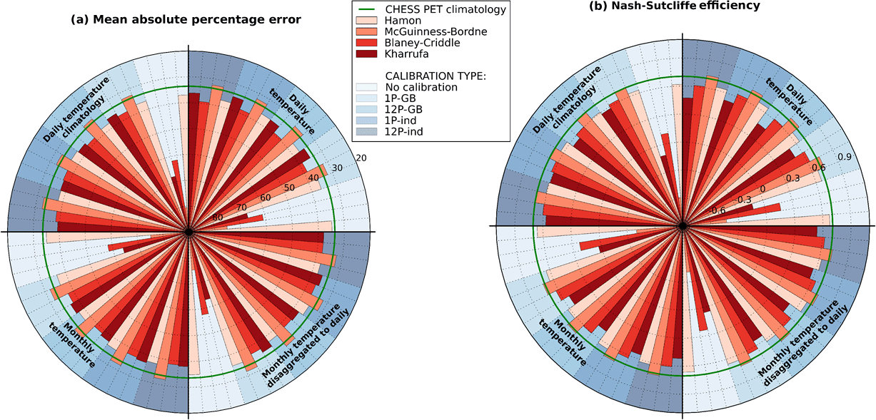
Figure 4 Performance of the different combinations of PET equations (shown in different shades of red), calibration approaches (shown in different shades of blue) and input temperature data (one in each quadrant). The green line on the plots shows the reference CHESS PET climatology for comparison. (a) Mean absolute percentage error (MAPE) – note that the y axis is inverted so that lower MAPE values (which indicate better performance) are shown towards the outside of the radial plot. (b) Nash–Sutcliffe efficiency (NSE); a higher NSE indicates better performance.

These six metrics were chosen as they assess different aspects of the modelled data. NSE looks as how much better our model is in predicting PET compared to the long-term average (climatology), MAPE gives an indication of the uncertainty, r informs about how well the modelled PET fits the observed values (or “proxy” to observed in our case), β tells us whether the estimations are biased, VR whether the spread of the estimated values matches the observed spread, and finally KGE informs on the combined effect of r, β and VR.

4 Results

4.1 Assessment of the temperature-based PET equations

In this section, results from the evaluation represented in stage 2 and 3 of Fig. 1 are presented.

Figure 4 is a summary graphic showing the average MAPE and NSE for all combinations of forcing data, PET equation and calibration strategy tested. For simplicity, Fig. 4 does not show the results from the following:

• models that were not calibrated in this study, i.e. Oudin, MOHYSE and Thornthwaite (Eqs. 5 to 7 in Table 2) (as these were performing worse than the calibrated models);

• using CHESS-temp monthly III forcing (similar results to those for CHESS-temp monthly II);

• using UKCP09-temp monthly I and II, as they were only used with the final selected equation as an additional test to check the effect of spatial resolution on the results (stage 3 in Fig. 1).

The full list of performance metrics is given in Tables S1 and S2 in the Supplement.

Figure 4 displays the following:

• i.

  Calibration yields substantial improvement in performance, except for Hamon (Eq. 1 in Table 2) which performed well before calibration.

• ii.

  Calibration strategy has very little effect on the performance. Both annual and global calibrations show a similar performance to the locally calibrated, monthly models. The simplest calibration approach was hence adopted: national-scale application was conducted using the 1P-GB strategy (see Fig. 3).

• iii.

  Daily temperature data only performs marginally better than forcing based on monthly temperature time series. This might be explained by the small day-to-day variability in temperature fields (and hence, in any resulting PET field) compared with other climate variables such as wind speed, humidity or radiation, which provide a much larger contribution to the daily variability of PET than temperature. The artificial daily pattern introduced by temporal disaggregation of monthly temperature is in fact small compared with the error introduced by using temperature-only forcing to estimate PET. This is illustrated in Fig. S1 (Supplement). Also, the temperature seasonal variability is a main component to the PET, and is well captured by monthly values, with sub-monthly values only adding some noise. This is why the choice of temperature data only has a marginal effect, because the daily variance is of secondary importance in comparison to an accurate representation of the seasonality.

• iv.

  CHESS-PM climatology is only outperformed by the calibrated version of McGuinness–Bordne equation (Eq. 2 in Table 2). This suggests a small inter-annual variability of PET, with a daily climatology being a good alternative when no other time series is available. Note however that the evaluation period (1991–2012) is too short for investigating the possible impact of trends (e.g. temperature trends, interdecadal variability, climate change signal) in the PET signal, which might reduce the overall ability of a climatology average to represent PET correctly. A surprising result is that, in the absence of any climate data available, calibrating the McGuinness–Bordne equation with CHESS-temp clim (long-term daily temperature climatology) outperforms using CHESS-PM climatology. NSE scores are equivalent for both approaches but MAPE is worse for the latter. The two approaches give similar results, but running the McGuinness–Bordne equation using CHESS-temp clim produces smoother time series than directly using CHESS-PM climatology. The latter displays random noise which explains the larger values of MAPE compared to the smoother version. This is illustrated in Fig. S4 in the Supplement.

A single annual McGuinness–Bordne PET equation calibrated over all catchments simultaneously was selected as the most appropriate method to derive daily PET time series from monthly mean temperature data.

To investigate the effect of coarser spatial resolution in the forcing temperature data, McGuinness–Bordne 1P-GB was applied using UKCP09-temp monthly I and II (5 km gridded data) as forcing data (stage 3 in Fig. 1). Results show (Table S1 in the Supplement) that at the catchment scale, the spatial resolution of the forcing temperature data has virtually no effect on the performance, with MAPE and NSE values almost identical when using 1 km gridded CHESS-temp monthly I data (MAPE = 32.02, NSE = 0.72) or 5 km gridded UKCP09-temp monthly I data (MAPE = 31.65, NSE = 0.72), and when using CHESS-temp monthly II data (MAPE = 32.13, NSE = 0.72) or UKCP09-temp monthly II data (MAPE = 32.06, NSE = 0.72). This suggests that for the reconstruction prior to 1961, when only 5 km monthly temperature time series are available across the UK, performance is expected to be equivalent to if finer spatial and temporal resolution of mean temperature data existed.

The relationship between performance and catchment area was also tested, but no clear relationship was found.

4.2 Assessment of the final PET grids

This section presents the results of the assessment described in stages 4 and 5 in Fig. 1.

Figure 5 Grids of evaluation metrics for the new daily gridded PET dataset. The darker the colour, the better the performance for all metrics represented, except for the bias ratio (β) (e) where the middle-range colour is optimal (see Sect. 3.3).

Based on the results in Sect. 4.1, the McGuinness–Bordne 1P-GB equation calibrated on 43 catchments was selected to generate a 5 km PET dataset covering the period 1891 to 2015, using UKCP09-temp monthly II data. A monthly version of the dataset (monthly aggregation of the daily PET for consistency) was also produced for applications requiring a coarse temporal resolution such as groundwater modelling, which has the advantage of a smaller data volume. The final gridded PET data produced here is hereafter referred to as “historic PET dataset”.

4.2.1 Catchment-scale calibration (stage 4, Fig. 1)

At catchment scale, there is virtually no difference in deriving PET time series from the historic PET dataset or from PET calculated with the same equation using catchment-average temperature. The correlation coefficient is close to 1 for the 306 catchments. This validates our assumption that the selected equation calibrated at catchment scale is applicable at grid scale.

4.2.2 Final evaluation (stage 5, Fig. 1)

PET extracted from the historic PET dataset was compared with CHESS-PM (ground truth), both at daily and monthly timescale, to evaluate the performance of the final reconstructed product, at catchment scale and grid scale.

At catchment scale, the results are more varied. Spatial differences can be observed between the different metrics and are represented in detail in Figs. S5 and S6 in the Supplement. The results are not discussed here as they are very similar to the grid-to-grid comparison described in the following.

Figure 6 Grids of evaluation metrics for the new monthly gridded PET dataset. The darker the colour, the better the performance for all metrics represented, except for the variability ratio (VR) (d) and bias ratio (β) (e) where the middle-range colour is optimal.

At the grid scale, the following observations can be made (Fig. 5 for daily PET and Fig. 6 for monthly PET; note differences in the legend colour scale):

• i.

  Performance is greater for monthly (Fig. 6) than daily (Fig. 5) PET, except for the bias ratio β which is very similar for both. This suggests that the error is greater at daily than at monthly resolution, likely to be due to the smoothing of the day-to-day variability absent in a temperature-based method. The PET equation shows very good performance at a monthly scale with values of NSE > 0.9, r > 0.97 and KGE > 0.8 for the whole country. For daily values, the performance is more moderate (NSE > 0.4, r > 0.8 and KGE > 0.7).

• ii.

  Performance varies spatially, but this variability depends on the metrics chosen and is different for monthly and daily PET. For daily PET, MAPE (Fig. 5a), NSE (Fig. 5b) and r (Fig. 5c) show lower performance near the coasts. This is probably because daily variation of wind and humidity are higher near the coast, which is not captured in temperature-based PET equations and hence results in larger errors. VR (Fig. 5d) displays a north–south gradient in performance, the north being better. This is because the coefficient of variability in observed PET is smaller in the north than it is in the south, with less daily noise (see Fig. S3 in the Supplement, grey line). The bias ratio β (Fig. 5e) is close to one everywhere across Great Britain, which indicates that the calibrated McGuinness–Bordne equation shows very little bias. KGE (Fig. 5f) which is a combination of r, VR and β, shows a north–south gradient as the strongest influence comes from VR. For monthly PET, the daily noise in the climate variables is absent, which explains smaller differences in performance scores for most metrics.

The metrics grids are provided as part of the dataset, and can inform the users on the quality of the PET estimation for a given location.

5 Data availability

The new PET dataset is called “Historic Gridded Potential Evapotranspiration (PET)” based on the temperature-based equation McGuinness–Bordne calibrated for the UK (1891–2015)” and is available from https://doi.org/10.5285/17b9c4f7-1c30-4b6f-b2fe-f7780159939c (Tanguy et al., 2017). The dataset is stored in NetCDF4 format.

For the monthly grids, the dataset is structured as three-dimensional grids covering the UK, with twelve time steps (monthly grids) in the time dimension in each yearly file, and a spatial resolution of 5 km.

For the daily grids, the dataset is structured as three-dimensional grids covering the UK, with 365 or 366 (leap year) time steps (daily grids) in each yearly file, and a spatial resolution of 5 km.

In addition, four metric files, also in NetCDF format, accompany the PET files (two for daily grids and two for monthly grids), also at a spatial resolution of 5 km.

The data are projected using the British National Grid co-ordinate system.

The following citation should be used for every application of the data: Tanguy, M., Prudhomme, C., Smith, K., and Hannaford, J.: Historic Gridded Potential Evapotranspiration (PET) based on temperature-based equation McGuinness–Bordne calibrated for the UK (1891–2015), NERC Environmental Information Data Centre, 2017.

The dataset is available for download from the CEH Environmental Information Data Centre (EIDC).

The temperature and PET datasets used in this study are available to download from the following links:

• CHESS temperature data (Robinson et al., 2016a) can be downloaded from the EIDC catalogue: https://catalogue.ceh.ac.uk/documents/b745e7b1-626c-4ccc-ac27-56582e77b900.

• CHESS PET data (Robinson et al., 2016b) can be downloaded from the EIDC catalogue: https://catalogue.ceh.ac.uk/documents/8baf805d-39ce-4dac-b224-c926ada353b7.

• UKCP09 temperature data (Perry and Hollis, 2005) can be downloaded from CEDA catalogue: http://catalogue.ceda.ac.uk/uuid/87f43af9d02e42f483351d79b3d6162a.

6 Discussion, limitations and recommendations

In this section, the uncertainties linked to the temperature dataset and the PET method are discussed. Subsequently, recommendations to users depending on the intended application of the data are listed. Lastly, a summary of findings and potential future work are presented.

6.1 Uncertainties

Firstly, the uncertainties linked to the underpinning temperature data should be considered. The data rescuing work that the UK Met Office has undertaken to extend the temperature data back to the late 19th century raises some questions about how the change in network density might affect the accuracy of the spatial data.

According to information provided by the Met Office, the station density gradually increased from 74 stations across the country in 1891 to a peak of 672 in the mid-1990s, after which it decreased again to reach a total of 355 stations in 2015. Legg (2015) has extensively investigated the effect of network density on the error in gridded dataset in the UK, and his results suggest that the change in density observed here would only lead to a minor increase in error in temperature. An increase in the root mean square error of less than 0.2 ^∘C is observed for most cases when the network density changes from 570 to 75 stations across the UK. This reflects the spatial coherence in the temperature data.

A sensitivity analysis of McGuinness–Bordne PET on errors in input temperature was conducted. It was found that a ±0.2 ^∘C in input temperature translates into a 0.5 to 2 % difference (with an average of 0.8 %) in PET estimation. We consider these differences negligible in comparison to the uncertainties arising from the PET method itself (MAPE ranging from 14 to 24 % for monthly PET estimation, see Fig. 6a).

Some additional considerations regarding the joining of the two temperature datasets can be found in the Supplement (Sect. S2).

The main limitation of the historic PET dataset comes from the method used to derive it, which only takes temperature into account. This is the case particularly for the daily version. The PM evapotranspiration equation has radiative and convective components. In simplified temperature-based equations, temperature is used as a proxy for radiation but does not account for the convective aspect. Therefore, temperature-based equations are not able to reproduce the full daily fluctuation of PET, and are only a smoothed version of reality. This has to be kept in mind for applications where the daily variability of PET is important, such as the estimation of daily water balance, flood peaks and crop water demand, among others. Users are strongly advised to look at performance metrics associated with the dataset in their study area, such as monthly MAPE for example, which provide information on the uncertainty in the estimates. Note that because of the absence of the reference dataset CHESS-PM in Northern Ireland, no quality metrics are available in that region. Datasets based on physically based equations such as CHESS-Penman–Monteith (CHESS-PM) are a better option when and where they are available, which is not the case in Great Britain before 1961, and in Northern Ireland. When and where such high-resolution physically based PET datasets are not available, temperature-based PET datasets such as the historical PET dataset reconstructed here provide a valuable substitute.

At a monthly timescale, the magnitude in the seasonal cycle is well captured, which is reflected in better performance metrics for the monthly PET data compared to the daily PET (Figs. 5 and 6). This makes this dataset particularly suitable for deriving monthly or seasonal river discharges or run-offs, as its accuracy is adequate at this coarser timescale, and its daily temporal resolution is sufficient for most hydrological modelling applications.

6.2 Applications

While uncertainties in the PET dataset are quite large, especially in the daily version, the impact it might have will depend on the intended purpose of the data.

For hydrological applications, the choice of PET equation was shown to affect the estimated streamflow when using hydrological models (Seiller and Anctil, 2016), in particular at high and low flows (Samadi, 2016). However, several studies show that hydrological models are much more sensitive to errors in rainfall than to errors in PET, especially in temperate climates such as the UK (Bastola et al., 2011; Guo et al., 2017; Paturel et al., 1995). Furthermore, other studies (Bai et al., 2016; Seiller and Anctil, 2016) show that hydrological model parameter calibration can eliminate the influences of different PET inputs on runoff simulations. Oudin et al. (2005) have also demonstrated that temperature-based methods are suitable for conceptual hydrological modelling, and when available at a fine spatial scale, are also suitable for distributed hydrological modelling. Therefore, the historic PET dataset is considered particularly suitable for use in hydrological models, especially if these are being calibrated using this dataset, as the impact of PET uncertainties will be small compared to those of rainfall. It's also worth mentioning that the McGuinness–Bordne equation used to derive the historic PET dataset was calibrated against CHESS-PM. There is no systematic bias (bias ratio ≈ 1, see Figs. 5 and 6) between the two datasets. The use of the historic PET data would therefore be adequate in hydrological models that have been calibrated using CHESS-PM, but recalibration would be recommended if any other PET source was used in the original calibration.

For macroecology and biogeography studies, Fisher Joshua et al. (2010) have produced a global “guide to choosing an ET model for geographical ecology”, according to the climate zone of the study area. For temperate climates such as the UK, their conclusion is that any PET model type (temperature-based, radiation-based or combination) is equally adequate for its use in biodiversity modelling. Therefore, the historic PET dataset would be appropriate for this type of application. However, for crop modelling, greater caution is required as modelled crop yield is highly sensitive to the choice of PET model (Balkovič et al., 2013; Liu et al., 2016; Luo et al., 2009).

Regarding the derivation of drought indices which use PET, some seem insensitive to the choice of PET model, such as the Reconnaissance Drought Index (Tsakiris et al., 2007) as demonstrated by Vangelis et al. (2013); whereas for others such as the Standardized Precipitation-Evapotranspiration Index (Vicente-Serrano et al., 2009) or the Palmer Drought Severity Index (Palmer, 1965), different formulations of PET have a significant impact on the result (Beguería et al., 2013; Sheffield et al., 2012; Stagge et al., 2014). However, this is less important in humid areas such as the UK (Beguería et al., 2013). Therefore, the impact of uncertainties in PET for deriving drought indices will depend on the choice of drought index.

In general, for the use of the historic PET dataset to derive drought indices, or any other application not mentioned above, we would recommend that the user compares the results over the more recent period (1961–2015) using (i) CHESS-PM and (ii) the historic PET dataset, to estimate the impact of PET uncertainties in their study. This way, the user can truly assess the sensitivity of their specific application to the errors in PET, investigate how the uncertainties propagate in their model and make an informed decision on whether the historic PET dataset is suitable for their needs or not.

6.3 Further findings and future work

Beyond generating a new 125 years gridded daily PET dataset for the UK, this research has highlighted valuable insights for PET calculation in the UK:

• i.

  calibration is essential for realistic results, but the choice of calibration method (global/annual or local/monthly) has a minimal effect, and therefore the easiest, most cost-effective calibration method is recommended (global/annual);

• ii.

  the temporal resolution of the input temperature data and the temporal disaggregation method when using monthly data has little influence on the results;

• iii.

  temperature-based equations perform better at a monthly scale than at a daily scale, as the full daily fluctuation of PET due to other climate variables (wind speed, humidity, radiation) are not being accounted for, but these are smoothed out at the monthly scale;

• iv.

  the temperature-based PET equation (from the seven equations tested) that produces the best results for the UK is the calibrated version of the McGuinness–Bordne equation;

• v.

  for this equation, the spatial resolution (1 or 5 km) of the input temperature data has virtually no effect in the results at catchment scale;

• vi.

  CHESS-PM daily climatology is the second best of the tested options, and is therefore a possible alternative source of PET if no climate variables are available. (Whilst mean seasonal PET or climatology can be used in hydrological modelling (Burnash, 1995; Calder et al., 1983; Fowler, 2002), McGuinness–Bordne derived PET time series are preferable as they are able to reproduce the inter-annual variability existing in PET, absent from any climatology); and finally,

• vii.

  performance of the McGuinness–Bordne equation across the UK is variable in space, and the gridded metrics provided within the dataset can inform future work on the adequacy of using this approach for estimating PET in particular areas.

Future research could explore the use of reanalysis data as an alternative or complementary source of data to derive past spatio-temporal PET data. The use of reanalysis data would enable the calculation of PET through the more accurate combined methods (such as PM). However, the uncertainties associated with reanalysis data should be carefully examined, as some of the modelled variables can display large errors (Reichler and Kim, 2008), and PM has also shown sensitivity to input data inaccuracy (Oudin et al., 2005; Debnath et al., 2015; Estévez et al., 2009; Gong et al., 2006).