A new bed elevation model for the Weddell Sea sector of the West Antarctic Ice Sheet

We present a new digital elevation model (DEM) of the bed, with a 1 km gridding, of the Weddell Sea (WS) sector of the West Antarctic Ice Sheet (WAIS). The DEM has a total area of ∼ 125 000 km² covering the Institute, Möller and Foundation ice streams, as well as the Bungenstock ice rise. In comparison with the Bedmap2 product, our DEM includes new aerogeophysical datasets acquired by the Center for Remote Sensing of Ice Sheets (CReSIS) through the NASA Operation IceBridge (OIB) program in 2012, 2014 and 2016. We also improve bed elevation information from the single largest existing dataset in the region, collected by the British Antarctic Survey (BAS) Polarimetric radar Airborne Science Instrument (PASIN) in 2010–2011, from the relatively crude measurements determined in the field for quality control purposes used in Bedmap2. While the gross form of the new DEM is similar to Bedmap2, there are some notable differences. For example, the position and size of a deep subglacial trough (∼ 2 km below sea level) between the ice-sheet interior and the grounding line of the Foundation Ice Stream have been redefined. From the revised DEM, we are able to better derive the expected routing of basal water and, by comparison with that calculated using Bedmap2, we are able to assess regions where hydraulic flow is sensitive to change. Given the potential vulnerability of this sector to ocean-induced melting at the grounding line, especially in light of the improved definition of the Foundation Ice Stream trough, our revised DEM will be of value to ice-sheet modelling in efforts to quantify future glaciological changes in the region and, from this, the potential impact on global sea level. The new 1 km bed elevation product of the WS sector can be found at https://doi.org/10.5281/zenodo.1035488.

1 Introduction

The Intergovernmental Panel on Climate Change (IPCC) concluded that global sea level rise may range from 0.26 to 0.82 m by the end of the 21st century (Stocker, 2014). The rising oceans pose a threat to the socio-economic activities of hundreds of millions of people, mostly in Asia, living at and close to the coastal environment. Several processes drive sea level rise (e.g. thermal expansion of the oceans), but the largest potential factor comes from the ice sheets in Antarctica. The West Antarctic Ice Sheet (WAIS), which if melted would raise sea level by around 3.5 m, is grounded on a bed which is in places more than 2 km below sea level (Bamber et al., 2009a; Ross et al., 2012; Fretwell et al., 2013), allowing the ice margin to have direct contact with ocean water. One of the most sensitive regions of the WAIS to potential ocean warming is the Weddell Sea (WS) sector (Ross et al., 2012; Wright et al., 2014). Ocean modelling studies show that changes in present ocean circulation could bring warm ocean water into direct contact with the grounding lines at the base of the Filchner–Ronne Ice Shelf (FRIS) (Hellmer et al., 2012; Wright et al., 2014; Martin et al., 2015; Ritz et al., 2015; Thoma et al., 2015), which would act in a manner similar to the ocean-induced basal melting under the Pine Island Glacier ice shelf (Jacobs et al., 2011). Enhanced melting of the FRIS could lead to a decrease in the buttressing support to the upstream grounded ice, causing enhanced flow to the ocean. A recent modelling study, using a general ocean circulation model coupled with a 3-D thermodynamic ice-sheet model, simulated the inflow of warm ocean water into the Filchner–Ronne Ice Shelf cavity on a 1000-year timescale (Thoma et al., 2015). A second modelling study, this time using an ice-sheet model only, indicated that the Institute and Möller ice streams are highly sensitive to melting at the grounding lines, with grounding-line retreat up to 180 km possible across the Institute and Möller ice streams (Wright et al., 2014). While the Foundation Ice Stream was shown to be relatively resistant to ocean-induced change (Wright et al., 2014), a dearth of geophysical measurements of ice thickness across the ice stream at the time means the result may be inaccurate.

The primary tool for measurements of subglacial topography and basal ice-sheet conditions is radio-echo sounding (RES) (Dowdeswell and Evans, 2004; Bingham and Siegert, 2007). The first topographic representation of the land surface beneath the Antarctic ice sheet (Drewry, 1983) was published by the Scott Polar Research Institute (SPRI), University of Cambridge, in collaboration with the US National Science Foundation Office of Polar Programs (NSF OPP) and the Technical University of Denmark (TUD), following multiple field seasons of RES surveying in the late 1960s and 1970s (Drewry and Meldrum, 1978; Drewry et al., 1980; Jankowski and Drewry, 1981; Drewry, 1983). The compilation included folio maps of bed topography, ice-sheet surface elevation and ice thickness. The bed was digitized on a 20 km grid for use in ice-sheet modelling (Budd et al., 1984). However, only around one-third of the continent was measured at a line spacing of less than ∼ 100 km, making the elevation product erroneous in many places, with obvious knock-on consequences for modelling. Several RES campaigns were thenceforth conducted, and data from them were compiled into a single new Antarctic bed elevation product, named Bedmap (Lythe et al., 2001). The Bedmap digital elevation model (DEM) was gridded on 5 km cells and included an over 1.4 million km and 250 000 km line track of airborne and ground-based radio-echo sounding data, respectively. Subglacial topography was extended north to 60^∘ S, for purposes of ice-sheet modelling and determination of ice–ocean interactions. Since its release, Bedmap has proved to be highly useful for a wide range of research, yet inherent errors within it (e.g. inaccuracies in the DEM and conflicting grounding lines compared with satellite-derived observations) restricted its effectiveness (Le Brocq et al., 2010). After 2001, several new RES surveys were conducted to fill data gaps revealed by Bedmap, especially during and after the fourth International Polar Year (2007–2009). These new data led to the most recent Antarctic bed compilation, named Bedmap2 (Fretwell et al., 2013). Despite significant improvements in the resolution and accuracy of Bedmap2 compared with Bedmap, a number of inaccuracies and poorly sampled areas persist (Fretwell et al., 2013; Pritchard, 2014), preventing a comprehensive appreciation of the complex relation between the topography and internal ice-sheet processes and indeed a full appreciation of the sensitivity of the Antarctic ice sheet to ocean and atmospheric warming.

The WS sector was the subject of a major aerogeophysical survey in 2010–2011 (Ross et al., 2012), revealing the ∼ 2 km deep Robin Subglacial Basin immediately upstream of present-day grounding lines, from which confirmation of the ice-sheet sensitivity from ice-sheet modelling was determined (Wright et al., 2014). Further geophysical surveying of the region has been undertaken since Bedmap2 (Ross et al., 2012), which has provided an enhanced appreciation of the importance of basal hydrology to ice flow (Siegert et al., 2016b) and complexities associated with the interaction of basal water flow, bed topography and ice-surface elevation (Lindbäck et al., 2014; Siegert et al., 2014; Graham et al., 2017), emphasizing the importance of developing accurate and high-resolution DEMs, both for the bed and the surface, in glaciology.

In this paper, we present an improved bed DEM for the WS sector, based on a compilation of new airborne radar surveys. The DEM has a total area of ∼ 125 000 km² and is gridded to 1 km cells. From this dataset, we reveal changes for the routing of subglacial melt water and discuss the differences between the new DEM and Bedmap2. Our new bed DEM can also be easily combined with updated surface DEMs to improve ice-sheet modelling and subglacial water pathways.

2 Study area

The WS sector covers the Institute, Möller and Foundation ice streams, as well as the Bungenstock ice rise (Fig. 1). The region covered by the DEM extends 135 km south of the Bungenstock ice rise, 195 km east of the Foundation Ice Stream, over the Pensacola Mountains and 185 km west of the Institute Ice Stream. In comparison with Bedmap2, our new DEM benefits from several new airborne geophysical datasets (e.g. NASA Operation IceBridge, OIB, 2012, 2014 and 2016). In addition, the new DEM is improved by the inclusion of ice thickness picks derived from synthetic aperture radar (SAR)-processed RES data from the British Antarctic Survey (BAS) aerogeophysical survey of the Institute and Möller ice streams conducted in 2010–2011. This has improved the accuracy of the determination of the ice–bed interface in comparison to Bedmap2. We used the Differential Interferometry Synthetic Aperture Radar (DInSAR) grounding line (Rignot et al., 2011c) to delimit the ice shelf-facing margin of our grid.

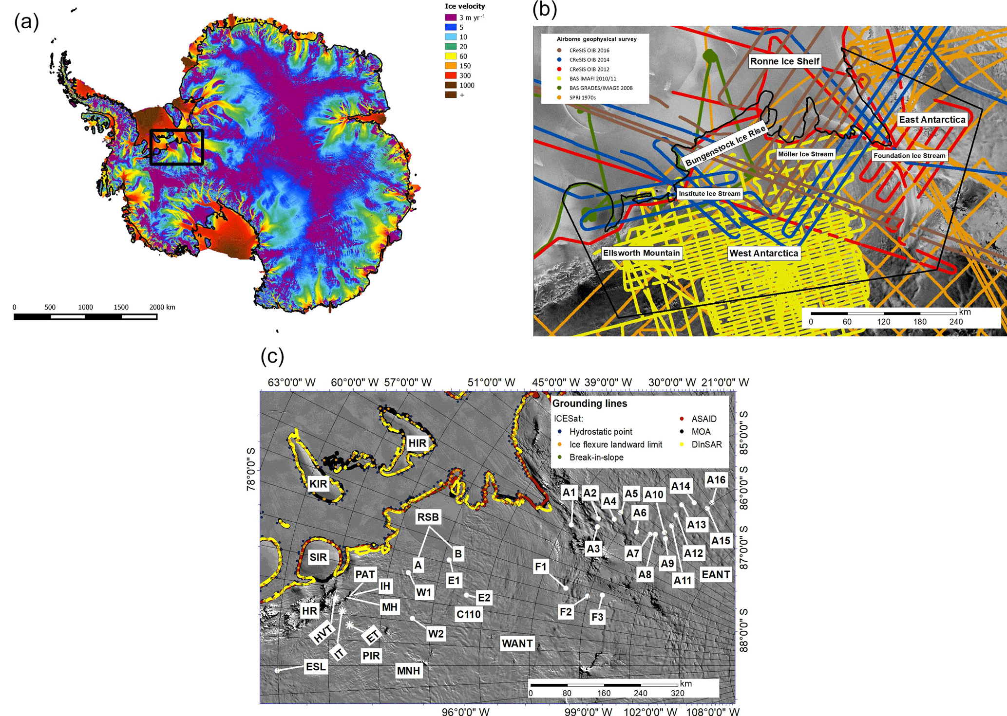
Figure 1 (a) Location of the study area overlain with InSAR-derived ice-surface velocities (Rignot et al., 2011d). (b) Aerogeophysical flight lines across the WS sector superimposed over RADARSAT (25 m) satellite imagery mosaic (Jezek, 2002); SPRI airborne survey 1969–1979 (orange); BAS GRADES/IMAGE survey 2008 (green); BAS Institute Ice Stream survey in 2010–2011 (IMAFI) (yellow); OIB 2012 (red); OIB 2014 (blue); and OIB 2016 (brown). (c) Map of the WS sector based on MODIS imagery (Haran et al., 2014) with grounding lines superimposed and denoted as follows: ICESat laser altimetry (blue: hydrostatic point; orange: ice flexure landward limit; green: break-in-slope) grounding line (Brunt et al., 2010), Antarctic Surface Accumulation and Ice Discharge (ASAID) grounding line (red line) (Bindschadler et al., 2011), Mosaic of Antarctica (MOA) grounding line (black line) (Bohlander and Scambos, 2007), and Differential Interferometry Synthetic Aperture Radar (DInSAR) grounding line (yellow line) (Rignot et al., 2011a). Annotations are as follows: KIR – Korff ice rise; HIR – Henry ice rise; SIR – Skytrain ice rise; HR – Heritage Range; HVT – Horseshoe Valley Trough; IT – Independence Trough; ET – Ellsworth Trough; ESL – Ellsworth Subglacial Lake; E1 – Institute E1 Subglacial Lake; E2 – Institute E2 Subglacial Lake; A1 – Academy 1 Subglacial Lake; A2 – Academy 2 Subglacial Lake; A3 – Academy 3 Subglacial Lake; A4 – Academy 4 Subglacial Lake; A5 – Academy 5 Subglacial Lake; A6 – Academy 6 Subglacial Lake; A7 – Academy 7 Subglacial Lake; A8 – Academy 8 Subglacial Lake; A9 – Academy 9 Subglacial Lake; A10 – Academy 10 Subglacial Lake; A11 – Academy 11 Subglacial Lake; A12 – Academy 12 Subglacial Lake; A13 – Academy 13 Subglacial Lake; A14 – Academy 14 Subglacial Lake; A15 – Academy 15 Subglacial Lake; A16 – Academy 16 Subglacial Lake; A17 – Academy 17 Subglacial Lake; W1 – Institute W1 Subglacial Lake; W2 Institute W2 Subglacial Lake; F1 – Foundation 1 Subglacial Lake; F2 – Foundation 2 Subglacial Lake; F3 – Foundation 3 Subglacial Lake; PAT – Patriot Hills; IH – Independence Hills; MH – Marble Hills; PIR – Pirrit Hills; MNH – Martin–Nash Hills; RSB – Robin Subglacial Basin; WANT – West Antarctica; EANT – East Antarctica.

3 Data and methods

The RES data used in this study were compiled from four main sources (Fig. 1a): first, SPRI data collected during six survey campaigns between 1969 and 1979 (Drewry, 1983); second, the BAS airborne radar survey accomplished during the austral summer 2006–2007 (known as GRADES/IMAGE: Glacial Retreat of Antarctica and Deglaciation of the Earth System/Inverse Modelling of Antarctica and Global Eustasy) (Ashmore et al., 2014); third, the BAS survey of the Institute and Möller ice streams, undertaken in 2010–2011 (Institute–Möller Antarctic Funding Initiative, IMAFI) (Ross et al., 2012); fourth, flights conducted by the Center for Remote Sensing of Ice Sheets (CReSIS) during the NASA OIB programme in 2012, 2014 and 2016 (Gogineni, 2012) supplement the data previously used in the Bedmap2 bed elevation product to accurately characterize the subglacial topography of this part of the WS sector.

3.1 Scott Polar Research Institute survey

The SPRI surveys covered a total area of 6.96 million km² (∼ 40 % of continental area) across West and East Antarctica (Drewry et al., 1980). The data were collected using a pulsed radar system operating at centre frequencies of 60 and 300 MHz (Christensen, 1970; Skou and Søndergaard, 1976) equipped on an NSF LC-130 Hercules aircraft (Drewry and Meldrum, 1978; Drewry et al., 1980; Jankowski and Drewry, 1981; Drewry, 1983). The 60 MHz antennas, built by the Technical University of Denmark, comprised an array of four half-wave dipoles, which were mounted in neutral aerofoil architecture of insulating components beneath the starboard wing. The 300 MHz antennas were composed of four dipoles attached underneath a reflector panel below the port wing. The purpose of this unique design was to improve the backscatter acquisition and directivity. The returned signals were archived on 35 mm film and dry-silver paper by a fibre optic oscillograph. Aircraft navigation was assisted using an LTN-51 inertial navigation system giving a horizontal positional error of around 3 km. Navigation and other flight data were stored on magnetic and analogue tape by an Airborne Research Data System (ARDS) constructed by the US Naval Weapons Center. The system recorded up to 100 channels of six-digit data with a sampling rate of 303 Hz per channel. Navigation, ice thickness and ice-surface elevation records were recorded every 20 s, corresponding to around 1.6 km between each data point included on the Bedmap2 product. The data were initially recorded on a 35 mm photographic film (i.e. Z-scope radargrams) and were later scanned and digitized, as part of a NERC Centre for Polar Observation and Modelling (CPOM) project, in 2004. Each film record was scanned separately and reformatted to form a single electronic image of a RES transect. The scanned image was loaded into an image analysis package (i.e. ERDAS Imagine) to trace the internal and the ice–bed interface which were then digitized. The digitized dataset was later standardized with respect to the ice surface.

3.2 BAS GRADES/IMAGE surveys

The GRADES/IMAGE project was conducted during the austral summer of 2006–2007 and acquired ∼ 27 550 km of airborne RES data across the Antarctic Peninsula, Ellsworth Mountains and Filchner–Ronne Ice Shelf. The BAS Polarimetric radar Airborne Science Instrument (PASIN) operates at a centre frequency of 150 MHz, has a 10 MHz bandwidth and a pulse-coded waveform acquisition rate of 312.5 Hz (Corr et al., 2007; Ashmore et al., 2014). The PASIN system interleaves a pulse and chirp signal to acquire two datasets simultaneously. Pulse data are used for imaging layering in the upper half of the ice column, whilst the more powerful chirp is used for imaging the deep ice and sounding the ice-sheet bed. The peak transmitted power of the system is 4 kW. The spatial sampling interval of ∼ 20 m resulted in ∼ 50 000 traces of data for a typical 4.5 h flight. The radar system consisted of eight folded dipole elements: four transmitters on the port side and four receivers on the starboard side. The receiving backscatter signal was digitized and sampled using a sub-Nyquist sampling technique. The pulses are compressed using a matched filter, and side lobes are minimized using a Blackman window. Aircraft position was recorded by an onboard carrier-wave global positioning system (GPS). The absolute horizontal positional accuracy for GRADES/IMAGE was 0.1 m (Corr et al., 2007). Synthetic aperture radar processing was not applied to the data.

3.3 BAS Institute–Möller Antarctic Funding Initiative surveys

The BAS data acquired during the IMAFI project consist of ∼ 25 000 km of aerogeophysical data collected during 27 flights from two field camps. A total of 17 flights were flown from C110, which is located close to Institute E2 Subglacial Lake, and the remaining 10 flights were flown from Patriot Hills (Fig. 1b). Data were acquired with the same PASIN radar used for the GRADES/IMAGE survey. The data rate of 13 Hz gave a spatial sampling interval of ∼ 10 m for IMAFI. The system was installed on the BAS de Havilland Twin Otter aircraft with a four-element folded dipole array mounted below the starboard wing used for reception and the identical array attached below the port wing for transmission. The flights were flown in a stepped pattern during the IMAFI survey to optimize potential field data (gravity and magnetics) acquisition (Fig. 1b). Leica 500 and Novatel DL-V3 GPS receivers were installed in the aircraft, corrected with two Leica 500 GPS base stations which were operated throughout the survey to calculate the position of the aircraft (Jordan et al., 2013). The positional data were referenced to the WGS 84 ellipsoid. The absolute positional accuracy for IMAFI (the standard deviation for the GPS positional error) was calculated to be 7 and 20 cm in the horizontal and vertical dimensions (Jordan et al., 2013). Two-dimensional focused SAR processing (Hélière et al., 2007) (see Sect. 4.1) was applied to the IMAFI data.

3.4 NASA OIB CReSIS surveys

The OIB project surveyed a total distance of ∼ 32 693, ∼ 52 460 and ∼ 53 672 km in Antarctica in 2012, 2014 and 2016, respectively, using the Multichannel Coherent Radar Depth Sounder (MCoRDS) system developed at the University of Kansas (Gogineni, 2012). The system was operated with a carrier frequency of 195 MHz and a bandwidth of 10 and 50 MHz in 2012 (Rodriguez-Morales et al., 2014) and 2014 onwards (Siegert et al., 2016b). The radar consisted of a five-element antenna array housed in a customized antenna fairing which is attached beneath the NASA DC–8 aircraft fuselage (Rodriguez-Morales et al., 2014). The five antennas were operated from a multichannel digital direct synthesis (DDS) controlled waveform generator enabling the user to adjust the frequency, timing, amplitude and phase of each transmitted waveform (Shi et al., 2010). The radar employs an eight-channel waveform generator to emit eight independent transmit chirp pulses. The system is capable of supporting five receiver channels with an Analog Devices AD9640 14 bit analogue-to-digital converter (ADC) acquiring the waveform at a rate of 111 MHz in 2012 (Gogineni, 2012). The system was upgraded in 2014 and 2016 utilizing six-channel chirp generation and supports six receiver channels with a waveform acquisition rate at 150 MHz. Multiple receivers allow array processing to suppress surface clutter in the cross-track direction which could potentially conceal weak echoes from the ice–bed interface (Rodriguez-Morales et al., 2014). The radar data are synchronized with the GPS and inertial navigation system (INS) using the GPS timestamp to determine the location of data acquisition.

4 Data processing

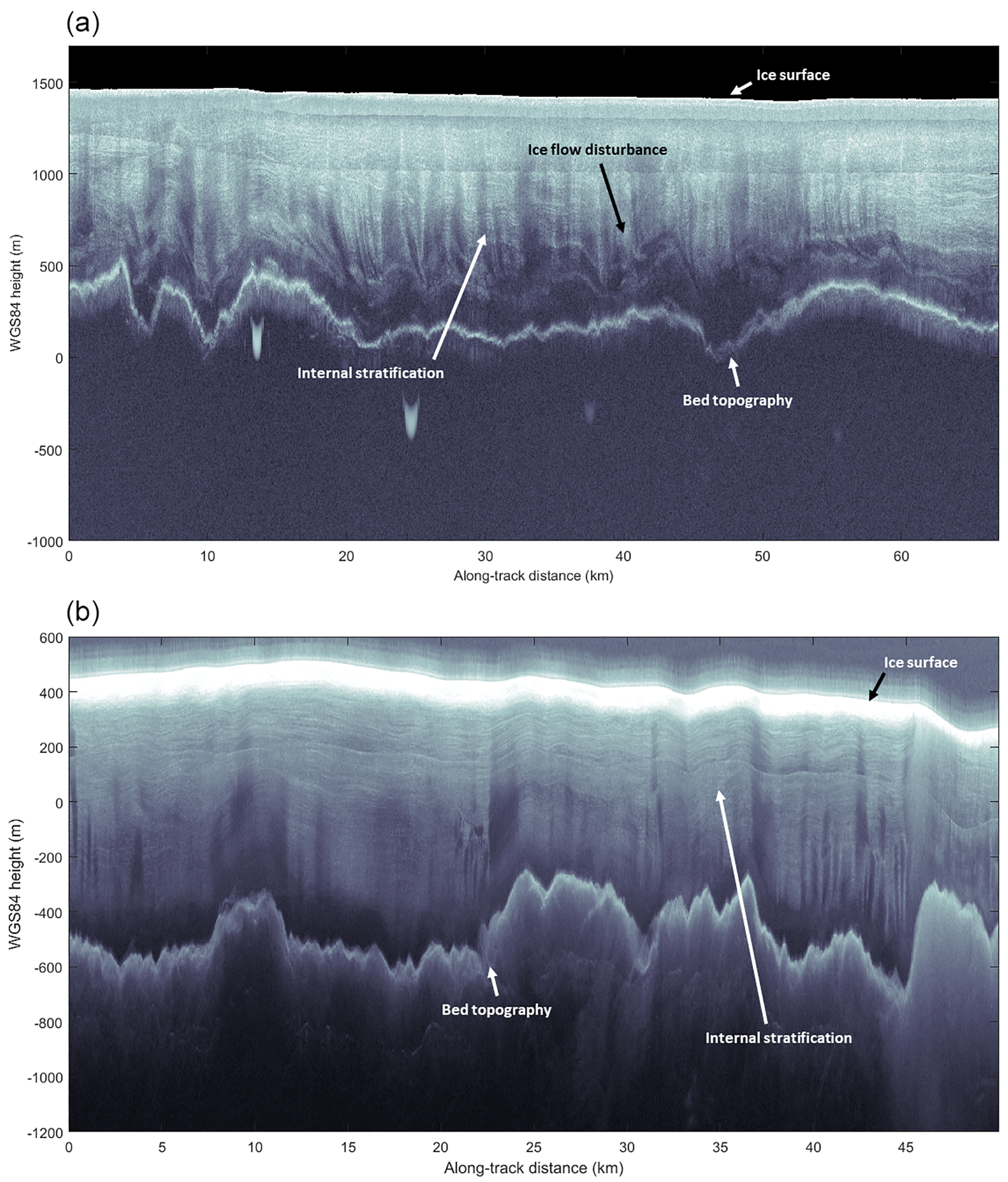
Figure 2 Two-dimensional synthetic aperture radar (SAR)-processed radargrams of (a) BAS IMAFI data and (b) OIB data.

We assume rain waves propagate through ice at a constant wave speed of 0.168 m ns⁻¹, which presupposes the ice to be homogenous (Gogineni et al., 2001, 2014; Lythe and Vaughan, 2001; Plewes and Hubbard, 2001; Dowdeswell and Evans, 2004). Low-density firn, ice chemistry and/or ice anisotropy (Diez et al., 2014; Fujita et al., 2014; Picotti et al., 2015; Shafique et al., 2016) violate this assumption, typically resulting in a depth bias of the order of ∼ 10 m. The radar pulse travels through a medium until it meets a boundary of differing dielectric constant, which causes some of the radio wave to be reflected and subsequently captured by the receiver antenna. The time travelled by the radar pulse between the upper and lower reflecting surface is measured and converted to ice thickness with reference to WGS 84 (Fig. 2). The digitized SPRI–NSF–TUD bed picks data are available through the BAS web page (https://data.bas.ac.uk/metadata.php?id=GB/NERC/BAS/AEDC/00326). The two-dimensional SAR-processed radargrams in SEG-Y format for the IMAFI survey are provided at https://doi.org/10.5285/8a975b9e-f18c-4c51-9bdb-b00b82da52b8, whereas the ice thickness datasets in comma-separated value (CSV) format for both GRADES/IMAGE and IMAFI are available via the BAS aerogeophysical processing portal (https://secure.antarctica.ac.uk/data/aerogeo/). The ice thickness data for IMAFI are provided in two folders: (1) the region of thinner ice (< 200 m) picked from the pulse dataset and (2) the overall ice thickness data, derived from picking of SAR-processed chirp radargrams. The data are arranged according to the latitude, longitude, ice thickness values and the pulse repetition interval radar shot number that is used to index the raw data. The OIB SAR images (level 1B) in MAT (binary MATLAB) format and the radar depth sounder level 2 (L2) data in CSV format are available via the CReSIS website (https://data.cresis.ku.edu/). The L2 data include measurements for GPS time during data collection, latitude, longitude, elevation, surface, bottom and thickness. For more information on these data, we refer the reader to the appropriate CReSIS guidance notes for each field season (i.e. https://data.cresis.ku.edu/data/rds/rds_readme.pdf).

4.1 GRADES/IMAGE and Institute–Möller Antarctic Funding Initiative data processing

The waveform was retrieved and sequenced according to its respective transmit pulse type. The modified data were then collated using MATLAB data binary files. Doppler filtering (Hélière et al., 2007) was used to remove the backscattering hyperbola in the along-track direction (Corr et al., 2007; Ross et al., 2012). Chirp compression was then applied to the along-track data. Unfocused synthetic aperture (SAR) processing was used for the GRADES/IMAGE survey by applying a moving average of 33 data points (Corr et al., 2007), whereas two-dimensional SAR (i.e. focused) processing based on the Omega-K algorithm was used to process the IMAFI data (Hélière et al., 2007; Winter et al., 2015) to enhance both along-track resolution and echo signal noise. The bed echo was depicted in a semi-automatic manner using ProMAX seismic processing software. All picking for IMAFI was undertaken by a single operator (Neil Ross). A nominal value of 10 m is used to correct for the firn layer during the processing of ice thickness, which introduces an error of the order of ±3 m across the survey field (Ross et al., 2012). This is small relative to the total error budget of the order of ±1 %. Finally, the GPS and RES data were combined to determine the ice thickness, ice-surface and bed elevation datasets. Elevations are measured with reference to WGS 84. The ice-surface elevation was calculated by subtracting terrain clearance from the height of the aircraft, whereas the bed elevation was computed by subtracting the ice thickness from the ice-surface elevation.

4.2 OIB data processing

The OIB radar adopts SAR processing in the along-track direction to provide higher-resolution images of the subglacial profile. The data were processed in three steps to improve the signal-to-noise ratio and increase the along-track resolution (Gogineni et al., 2014). The raw data were first converted from a digital quantization level to a receiver voltage level. The surface was captured using the low-gain data, microwave radar or laser altimeter. A normalized matched filter with frequency-domain windowing was then used for pulse compression. Two-dimensional SAR processing was used after conditioning the data, which is based on the frequency-wavenumber (F-K) algorithm. The F-K SAR processing requires straight and uniformly sampled data, however, which in the strictest sense are not usually met in the raw data since the aircraft's speed is not consistent and its trajectory is not straight. The raw data were thus spatially resampled along track using a sinc kernel to approximate a uniformly sampled dataset. The vertical deviation in aircraft trajectory from the horizontal flight path was compensated for in the frequency domain with a time-delay phase shift. The phase shift was later removed for array processing as it is able to account for the non-uniform sampling; the purpose is to maintain the original geometry for the array processing. Array processing was performed in the cross-track flight path to reduce surface clutter as well as to improve the signal-to-noise ratio. Both the delay-and-sum and minimum variance distortionless response (MVDR) beamformers were used to combine the multichannel data, and for regions with significant surface clutter the MVDR beamformer could effectively minimize the clutter power and pass the desired signal with optimum weights (Harry and Trees, 2002).

4.3 Quantifying ice thickness, bed topography and subglacial water flow

The new ice thickness DEM was formed from the RES data using the “Topo to Raster” function in ArcGIS, based on the Australian National University DEM (ANUDEM) elevation gridding algorithm (Hutchinson, 1988). This is the same algorithm employed by Bedmap2. The ice thickness DEM was then subtracted from the ice-sheet surface elevation DEM (from European Remote Sensing Satellite-1 (ERS-1) radar and Ice, Cloud and land Elevation Satellite (ICESat) laser satellite altimetry datasets, Bamber et al., 2009b) to derive the bed topography. The ice thickness, ice-sheet surface and bed elevations were then gridded at a uniform 1 km spacing and referenced to the polar stereographic projection (Snyder, 1987) to form the new DEMs. The Bedmap2 bed elevation product (Fretwell et al., 2013) was transformed from the gl04c geoid projection to the WGS 1984 Antarctic Polar Stereographic projection for comparison purposes. A difference map between the new DEM and the Bedmap2 product was computed by subtracting the Bedmap2 bed elevation DEM from the new bed elevation DEM. Crossover analysis for the 2006–2007 data onwards (including data acquired on flight lines beyond the extent of our DEM) shows the RMS errors of 9.1 m (GRADES/IMAGE), 15.8 m (IMAFI), 45.9 m (CRESIS 2012), 23.7 m (CRESIS 2014) and 20.3 m (CRESIS 2016).

Subglacial water flow paths were calculated based on the hydraulic potentiometric surface principle, in which basal water pressure is balanced by the ice overburden pressure as follows:

$$\begin{array}{}\text{(1)}& \mathit{\phi }=g({\mathit{\rho }}_{\mathrm{w}}y+{\mathit{\rho }}_{\mathrm{i}}h),\end{array}$$

where φ is the theoretical hydropotential surface; y is the bed elevation; h is the ice thickness; ρ_w and ρ_i are the density of water (1000 kg m⁻³) and ice (920 kg m⁻³), assuming ice to be homogenous, respectively; and g is the gravitational constant (9.81 m s⁻²) (Shreve, 1972). Sinks in the hydrostatic pressure field raster were filled to produce realistic hydrologic flow paths. The flow direction of the raster was then defined by assigning each cell a direction to the steepest downslope neighbouring cell. Sub-basins less than 200 km² were removed due to the coarse input of bed topography and ice thickness DEMs.

4.4 Inferring bed elevation using mass conservation (MC) and kriging

Relying on the conservation of mass (MC) to infer the bed between flight lines (Morlighem et al., 2011), we were able to investigate how the bed can be developed further in fast-flowing regions, using a new interpolation technique. To perform the MC procedure, we used InSAR-derived surface velocities (Fig. 1a) from Rignot et al. (2011b), surface mass balance from RACMO 2.3 (Regional Atmospheric Climate Model, Van Wessem et al., 2014), and assumed that the ice thinning–thickening rate and basal melt are negligible. We constrained the optimization with ground-penetrating radar from CReSIS, GRADES, IMAFI and SPRI, described above, and used a mesh horizontal resolution of 500 m.

5 Results

5.1 A new 1 km DEM of the WS sector

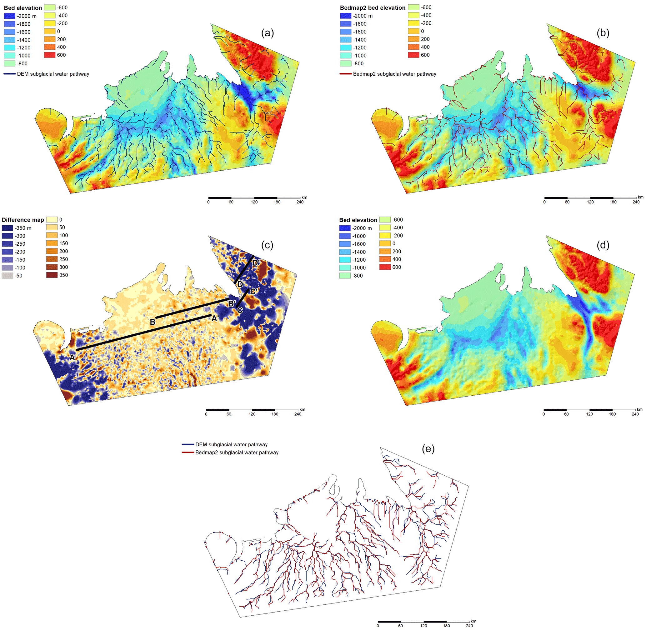
Figure 3 (a) The new bed DEM for the WS sector; (b) Bedmap2 bed elevation product (Fretwell et al., 2013); pathways of subglacial water are superimposed in (a) and (b). (c) Profiles A–A^′, B–B^′, C–C^′ and D–D^′ overlain by a map showing differences in bed elevation between the new DEM and Bedmap2; (d) bed DEM inferred using mass conservation and kriging; and (e) subglacial water pathways calculated with the new DEM (blue) and Bedmap2 (red).

We present a new DEM of the WS sector of West Antarctica (Fig. 3a). The Bedmap2 bed elevation and the difference map are shown in Fig. 3b and c, respectively. The new DEM contains substantial changes in certain regions compared with Bedmap2, whereas in others there are consistencies between the two DEMs, for example across the Bungenstock ice rise, where there are little new data. The mean error between the two DEMs is −86.45 m, indicating a slightly lower bed elevation in the new DEM data compared to Bedmap2, which is likely the result of deep parts of the topography (i.e. valley bottoms) not being visible in the fieldwork non-SAR-processed quality-control (QC) radargrams from the IMAFI project (e.g. Horseshoe Valley, near Patriot Hills in the Ellsworth Mountains; Winter, 2016). The bed elevation upstream of the Bungenstock ice rise and across the Robin Subglacial Basin shows a generally good agreement with Bedmap2, with only small areas across the Möller Ice Stream and Pirrit Hills significantly different from Bedmap2, with differences in bed elevation typically ranging between −109 and 172 m (Fig. 3c). There is, however, large disagreement between the two DEMs in the western region of Institute Ice Stream, across the Ellsworth Mountains (e.g. in the Horseshoe valley), the Foundation Ice Stream and towards East Antarctica where topography is more rugged. It is also worth noting the significant depth of the bed topography beneath the trunk of the Foundation Ice Stream, where a trough more than ∼ 2 km deep is located and delineated (Fig. 3a). The trough is ∼ 38 km wide and ∼ 80 km in length, with the deepest section ∼ 2.3 km below sea level. The new DEM shows a significant change in the depiction of Foundation Trough; we have measured it to be ∼ 1 km deeper and far more extensive relative to the Bedmap2 product.

In order to further quantify the differences between Bedmap2 and our new DEM, we present terrain profiles of both DEMs relative to four RES flight lines (Fig. 3c). The new DEM is consistent with the bed elevations from the RES data picks compared to Bedmap2 (Fig. 4a and b). The new DEMs show a correlation coefficient of 0.96 and 0.92 for Profile A and B, respectively. This is higher compared with Bedmap2 which is 0.94 (Profile A) and 0.91 (Profile B), with relative errors of 2 and 1 % for Profile A and B, respectively. Although inaccuracies of the bed elevation persist across the Foundation Ice Stream for both DEMs, the gross pattern of the bed elevation for the new DEM is more consistent with the RES transects relative to Bedmap2 (Fig. 4c and d), with correlation coefficients of 0.97 and 0.94 for Profile C and D, respectively. These values contrast with correlation coefficients from Bedmap2 of 0.87 for Profile C and 0.83 for Profile D, with relative errors of 12 and 13 %, respectively.

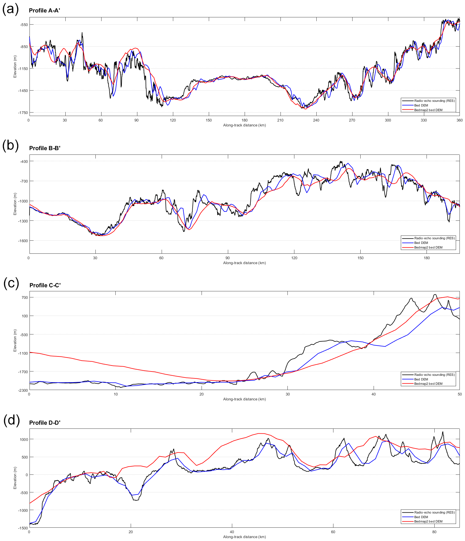
Figure 4 Bed elevations for RES transects (black), DEM (blue) and Bedmap2 (red) for (a) Profile A–A^′, (b) Profile B–B^′, (c) Profile C–C^′ and (d) Profile D–D^′.

The new DEM can be refined further to deal with bumps and irregularities associated with interpolation effects from along-track data in otherwise data-sparse regions. We used the (MC) technique to infer the bed elevation (Fig. 3d) beneath the fast-moving ice, similar to that employed in Greenland (Morlighem et al., 2017). In general, the bed elevation derived from MC and kriging is consistent with our new DEM. However, using MC, significant changes in the bed morphology beneath fast-flowing ice occur. For example, using MC, the tributary of the Foundation Ice Stream has been extended for ∼ 100 km further inland relative to our new DEM.

5.2 Hydrology

Computing the passageway of subglacial water beneath the ice sheet is critical for comprehending ice-sheet dynamics (Bell, 2008; Stearns et al., 2008; Siegert et al., 2016a). The development of subglacial hydrology pathways is highly sensitive to ice-surface elevation and, to a lesser degree, to bed morphology (Wright et al., 2008; Horgan et al., 2013). Figure 3e shows a comparison of subglacial hydrology pathways between our new bed DEM and the Bedmap2 DEM. The gross patterns of water flow are largely unchanged between the two DEMs, especially across and upstream of Institute and Möller ice streams. The similar water pathway pattern between both DEMs in these regions is also consistent with the small errors in bed topography (Fig. 3c). Despite large differences in bed topography across the Foundation Ice Stream and the Ellsworth Mountains region, the large-scale patterns of water flow are also similar between both DEMs, due to the dominance of the ice-surface slope in driving basal water flow in these regions (Shreve, 1972). Nonetheless, there are several local small-scale differences in the water pathways (Fig. 3e), which highlight hydraulic sensitivity. The subglacial water network observed in the new DEM across the Foundation Ice Stream appears to be more arborescent than that derived from Bedmap2. This is due to the introduction of new data, resulting in a better-defined bed across the Foundation Trough (Fig. 3a). The subglacial water pathway observed in the new DEM adjacent to the grounding line across the Möller Ice Stream is in good agreement with the position of sub-ice-shelf channels, which have been delineated from a combination of satellite images and RES data (Le Brocq et al., 2013).

Subglacial lakes discovered across the WS sector form an obvious component of the basal hydrological system (Wright and Siegert, 2012). These lakes exist due to sufficient amount of geothermal heating (50–70 m W m⁻²), which allows the base of the ice sheet to melt especially in areas of thick ice. In addition, the pressure exerted on the bed by the overlying ice causes the melting point to be lowered. West of the Ellsworth Mountains lies a body of the subglacial water known as Ellsworth Subglacial Lake. The lake measures 28.9 km² with a depth ranging between 52 and 156 m capable of carrying a water body volume of 1.37 km³ (Woodward et al., 2010). In some cases, ice-surface elevation changes have been linked with subglacial lake hydrological change (Siegert et al., 2016a) – referred to as “active” subglacial lakes. There are four known active subglacial lakes distributed across the Institute Ice Stream (Wright and Siegert, 2012): Institute W1 is located close to the Robin Subglacial Basin A whereas Institute W2 is located to the northeast of Pirrit Hills; Institute E1 and E2 are located to the southwest of Robin Subglacial Basin B and near the field camp of C110, respectively. There are three active subglacial lakes in the Foundation Ice Stream catchment: Foundation 1, Foundation 2 and Foundation 3 (Wright and Siegert, 2012). East of the Foundation Ice Stream, there are 16 active subglacial lakes distributed along the main trunk of Academy Glacier (Wright and Siegert, 2012).

5.3 Geomorphological description of the bed topography

The WS sector of WAIS is composed of three major ice-sheet outlets (Fig. 1a and b): the Institute, Möller and Foundation ice streams, feeding ice to the FRIS, the second largest ice shelf in Antarctica. Geophysical data in this area reveal features such as steep reverse bed slopes, similar in scale to that measured for upstream Thwaites Glacier, close to the Institute and Möller Ice Stream grounding lines. The bed slopes inland to a ∼ 1.8 km deep basin (the Robin Subglacial Basin), which is divided into two sections with few obvious significant ice-sheet pinning points (Ross et al., 2012). Elevated beds in other parts of the WS sector allow the ice shelf to ground, causing ice-surface features known as ice rises and rumples (Matsuoka et al., 2015).

Table 1 Data files and locations.

The Institute Ice Stream has three tributaries, within our survey grid, to the south and west of the Ellsworth Mountains, occupying the Horseshoe Valley, Independence and Ellsworth troughs (Fig. 1c) (Winter et al., 2015). The Horseshoe Valley Trough, around 20 km wide and 1.3 km below sea level at its deepest point, is located downstream of the steep mountains of the Heritage Range. A subglacial ridge is located between the mouth of the Horseshoe Valley Trough and the main trunk of the Institute Ice Stream (Winter et al., 2015). The Independence Trough is located subparallel to the Horseshoe Valley Trough, separated by the 1.4 km high Independence Hills. The trough is ∼ 22 km wide and is 1.1 km below sea level at its deepest point. It is characterized by two distinctive plateaus (∼ 6 km wide each) on each side of the trough, aligned alongside the main trough axis. Ice flows eastward through the Independence Trough for ∼ 54 km before it shifts to a northward direction where the trough widens to 50 km and connects with the main Institute Ice Stream. The Ellsworth Trough is aligned with the Independence Trough, and both are orthogonal to the orientation of the Amundsen–Weddell ice divide, dissecting the Ellsworth Subglacial Highlands northwest to southeast. The Ellsworth Trough measures ∼ 34 km in width, and is ∼ 2 km below sea level at its deepest point and is ∼ 260 km in length. It is considered to be the largest and deepest trough-controlled tributary in this region (Winter et al., 2015). The Ellsworth Trough is intersected by several smaller valleys aligned perpendicularly to the main axis, which are relic landforms from a previous small dynamic ice mass (predating the WAIS in its present configuration) (Ross et al., 2014). The Ellsworth Trough contains the ∼ 15–20 km long Ellsworth Subglacial Lake (Siegert et al., 2004a, 2012; Woodward et al., 2010; Wright and Siegert, 2012). It is worth noting that the lake is outside the grid of our DEM.

Satellite altimetry and imagery are able to estimate the grounding line that separates the grounded ice sheet from the floating ice shelf, based on surface changes due to tidal oscillations and the subtle ice-surface features. Such analysis is prone to uncertainty, however. There are currently four proposed grounding-line locations, based on different satellite datasets and/or methods of analysis (Bohlander and Scambos, 2007; Bindschadler et al., 2011; Brunt et al., 2011; Rignot et al., 2011c). Each of the grounding lines were delineated from satellite images but without direct measurement of the subglacial environment. This results in ambiguities for the grounding-line location (Jeofry et al., 2017a). In addition, RES data have demonstrated clear errors in the position of the grounding line with a large, hitherto unknown, subglacial embayment near the Institute Ice Stream grounding line. The subglacial embayment is ∼ 1 km deep and is potentially open to the ice shelf cavity, causing the inland ice sheet to have a direct contact with ocean water. Our RES analysis also reveals a better-defined Foundation Trough, in which the grounding line is perched on very deep topography around 2 km below sea level.

A previous study revealed a series of ancient large sub-parallel subglacial bed channels between Möller Ice Stream and Foundation Ice Stream, adjacent to the marginal basins (Fig. 1b) (Rose et al., 2014). While these subglacial channels are likely to have been formed by the flow of basal water, they are presently located beneath slow-moving and cold-based ice. It is thought, therefore, that the channels are ancient and were formed at a time when surface melting was prevalent in West Antarctica (e.g. the Pliocene).

The bed topography of the WS appears both rough (over the mountains and exposed bedrock) and smooth (across the sediment-filled regions) (Bingham and Siegert, 2007). Studies of bed roughness calculated using the fast Fourier transform (FFT) technique based on the relative measurement of bed obstacle amplitude and frequency of the roughness obstacles have indicated that the Institute Ice Stream and Möller Ice Stream are dominated by relatively low roughness values, less than 0.1 (Bingham and Siegert, 2007; Rippin et al., 2014), which was suggested as being the result of the emplacement of marine sediments as in the Siple Coast region (Siegert et al., 2004b; Peters et al., 2005). Radar-derived roughness analysis has evidenced a smooth bed across the Robin Subglacial Basin where sediments may exist (Rippin et al., 2014). The deepest parts of the Robin Subglacial Basin are anomalously rough, marking the edge of a sedimentary drape where the highest ice flow velocities are generated (Siegert et al., 2016b). As such, the smooth basal topography of the Institute and Möller Ice Stream catchments is less extensive than proposed by Bingham and Siegert (2007). The subglacial topography of the region between the Robin Subglacial Basin and the Pirrit and Martin–Nash Hills is relatively flat, smooth, and gently sloping and has been interpreted as a bedrock planation surface (Rose et al., 2015). Although the exact formation process of the planation surface is unknown, it is thought that this geomorphological feature formed due to marine and/or fluvial erosion (Rose et al., 2015).

6 Data availability

The new 1 km bed elevation product of the WS sector can be found at https://doi.org/10.5281/zenodo.1035488. We used four radar datasets to construct the 1 km ice thickness DEM, as follows: (1) digitized radar data from the 1970s SPRI–NSF–TUD surveys, in which the bed was picked every 15–20 s (1–2 km), recorded here in an Excel 97–2003 Worksheet (XLS), which can be obtained from the UK Polar Data Centre (UKPDC) website at https://data.bas.ac.uk/metadata.php?id=GB/NERC/BAS/AEDC/00326; (2) BAS GRADES/IMAGE and (3) BAS IMAFI airborne surveys, both available from the UKPDC Polar Airborne Geophysics Data Portal at https://secure.antarctica.ac.uk/data/aerogeo/; and (4) NASA Operation IceBridge radar depth sounder level 2 (L2) data, available from the Center for Remote Sensing of Ice Sheet (CReSIS) website at https://data.cresis.ku.edu/.

The 1 km ice-sheet surface elevation DEM was derived from a combination of ERS-1 surface radar and ICESat laser altimetry, which is downloadable from the National Snow and Ice Data Center (NSIDC) website at https://nsidc.org/data/docs/daac/nsidc0422_antarctic_1km_dem/. Newer surface elevation models (i.e. Helm et al., 2014) can easily be combined with our improved bed DEM.

Two-dimensional SAR-processed radargrams in SEG-Y format for the BAS IMAFI airborne survey and the NASA Operation IceBridge SAR images (level 1B) in MAT (binary MATLAB) format are provided at https://doi:10.5285/8a975b9e-f18c-4c51-9bdb-b00b82da52b8 and https://data.cresis.ku.edu/, respectively.

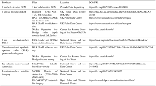
Ancillary information for the MEaSUREs InSAR-based ice velocity map of central Antarctica can be found at https://doi:10.5067/MEASURES/CRYOSPHERE/nsidc-0484.001 and the MODIS Mosaic of Antarctica 2008–2009 (MOA 2009) ice-sheet-surface image map is available at https://doi.org/10.7265/N5KP8037. The RADARSAT (25 m) ice-sheet-surface satellite imagery is accessible from the Byrd Polar and Climate Research Center website at https://research.bpcrc.osu.edu/rsl/radarsat/data/ (Byrd Polar and Climate Research Center, 2012). A summary of the data used in this paper and their availability is provided in the Table 1.

7 Conclusions

We have compiled airborne radar data from a number of geophysical surveys, including the SPRI–NSF–TUD surveys of the 1970s; the GRADES/IMAGE and IMAFI surveys acquired by BAS in 2006–2007 and 2010–2011, respectively; and new geophysical datasets collected by CReSIS from the NASA OIB project in 2012, 2014 and 2016. From these data, we produce a bed topography DEM which is gridded to 1 km postings. The DEM covers an area of ∼ 125 000 km² of the WS sector including the Institute, Möller and Foundation ice streams, as well as the Bungenstock ice rise. Large differences can be observed between the new and previous DEMs (i.e. Bedmap2), most notably across the Foundation Ice Stream where we reveal the grounding line to be resting on a bed ∼ 2 km below sea level, with a deep trough immediately upstream as deep as 2.3 km below sea level. In addition, improved processing of existing data better resolves deep regions of bed compared to Bedmap2. Our new DEM also revises the pattern of potential basal water flow across the Foundation Ice Stream and towards East Antarctica in comparison to Bedmap2. Our new DEM and the data used to compile it are available to download and will be of value to ice-sheet modelling experiments in which the accuracy of the DEM is important to ice flow processes in this particularly sensitive region of the WAIS.