the Creative Commons Attribution 4.0 License.
the Creative Commons Attribution 4.0 License.
 | 12 Mar 2018
A global space-based stratospheric aerosol climatology: 1979–2016
Nicholas Ernest
Luis Millán
Landon Rieger
Adam Bourassa
Jean-Paul Vernier
Gloria Manney
Beiping Luo
Florian Arfeuille
Thomas Peter
We describe the construction of a continuous 38-year record of stratospheric aerosol optical properties. The Global Space-based Stratospheric Aerosol Climatology, or GloSSAC, provided the input data to the construction of the Climate Model Intercomparison Project stratospheric aerosol forcing data set (1979–2014) and we have extended it through 2016 following an identical process. GloSSAC focuses on the Stratospheric Aerosol and Gas Experiment (SAGE) series of instruments through mid-2005, and on the Optical Spectrograph and InfraRed Imager System (OSIRIS) and the Cloud-Aerosol Lidar and Infrared Pathfinder Satellite Observation (CALIPSO) data thereafter. We also use data from other space instruments and from ground-based, air, and balloon borne instruments to fill in key gaps in the data set. The end result is a global and gap-free data set focused on aerosol extinction coefficient at 525 and 1020 nm and other parameters on an “as available” basis. For the primary data sets, we developed a new method for filling the post-Pinatubo eruption data gap for 1991–1993 based on data from the Cryogenic Limb Array Etalon Spectrometer. In addition, we developed a new method for populating wintertime high latitudes during the SAGE period employing a latitude-equivalent latitude conversion process that greatly improves the depiction of aerosol at high latitudes compared to earlier similar efforts. We report data in the troposphere only when and where it is available. This is primarily during the SAGE II period except for the most enhanced part of the Pinatubo period. It is likely that the upper troposphere during Pinatubo was greatly enhanced over non-volcanic periods and that domain remains substantially under-characterized. We note that aerosol levels during the OSIRIS/CALIPSO period in the lower stratosphere at mid- and high latitudes is routinely higher than what we observed during the SAGE II period. While this period had nearly continuous low-level volcanic activity, it is possible that the enhancement in part reflects deficiencies in the data set. We also expended substantial effort to quality assess the data set and the product is by far the best we have produced. GloSSAC version 1.0 is available in netCDF format at the NASA Atmospheric Data Center at https://eosweb.larc.nasa.gov/. GloSSAC users should cite this paper and the data set DOI (https://doi.org/10.5067/GloSSAC-L3-V1.0).
- Article
(18183 KB) - Full-text XML
- BibTeX
- EndNote


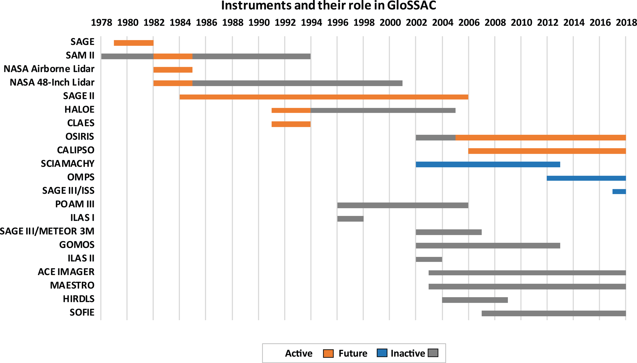
Figure 1Space-based sources for stratospheric aerosol extinction coefficient data and their status in GloSSAC. Two non-space instruments whose data are used in GloSSAC (NASA Airborne Lidar and NASA 48-inch lidar) are also shown.
Since the discovery of the stratospheric aerosol layer, there has been a continuing interest in the role of stratospheric aerosol in chemistry and climate. Stratospheric aerosol climatologies derived primarily from space-based observations of their optical properties have been key elements of the study of the effects of major volcanic events. Often, data sets covering the years following the 1991 eruption of Mount Pinatubo were developed based primarily on observations by the Stratospheric Aerosol and Gas Experiment (SAGE II)1 and other members of this series of instruments (see Fig. 1). We supplement SAGE observations with a variety of other space-based observations as well as ground- and balloon-based observations. These merged data have formed a part of a number of well-known aerosol climatologies including the Goddard Institute for Space Studies (GISS) Stratospheric Aerosol Optical Thickness forcing data set (Sato et al., 1993) and more extensive sets reported in Thomason et al. (1997b), Stenchikov et al. (1998), Bauman et al. (2003), SPARC (2006), and Arfeuille et al. (2013). These climatologies have been a part of a number of climate studies by individual users as well as larger group efforts such as the Climate Model Intercomparison Project (CMIP; Taylor et al., 2012).
Herein, we report on a global space-based stratospheric aerosol climatology (GloSSAC) that we developed to support the Coupled Model Intercomparison Project phase 6 (CMIP6; Morgenstern et al., 2017). GloSSAC is most closely related to the Assessment of Stratospheric Aerosol Properties (ASAP; SPARC, 2006) and CMIP phase 5 data sets (for papers related to this data set see Vernier et al., 2011, Solomon et al., 2011, and Mills et al., 2016) and follows the same basic paradigm that produce those versions. We build it primarily using space-based measurements by a number of instruments including the SAGE series, the Optical Spectrograph and InfraRed Imager System (OSIRIS; Rieger et al., 2015), the Cloud-Aerosol Lidar and Infrared Pathfinder Satellite Observation (CALIPSO; Vernier et al., 2011), Cryogenic Limb Array Etalon Spectrometer (CLAES; Massie et al., 1996), and the Halogen Occultation Experiment (HALOE; Thomason, 2012). We compile the data set in monthly depictions for 80∘ S to 80∘ N and from the tropopause to 40 km. We use the mean World Meteorological Organization tropopause (World Meteorological Organization, 1992) as a function of latitude and month as derived from MERRA for the SAGE II lifetime throughout this analysis. We preserve the tropopause data set within GloSSAC. The data set primarily consists of measurements by the instruments at their native wavelength and measurement type (e.g., extinction coefficient). However, every stratospheric bin in these monthly grids receives measured or indirectly inferred values for aerosol extinction coefficient at 525 and 1020 nm. Generally, when no data are available, bins are filled via simple linear interpolation in time only. The exceptions are in the SAGE I/II gap (1982–1984) where data from SAM II and ground-based and airborne lidar data sets are used. Ground-based lidar also supplements space-based data in the months following the Pinatubo eruption when much of the lower stratosphere was too optically opaque for SAGE II to measure. This data set includes total aerosol surface area density and volume estimates based on Thomason et al. (2008) (including size distribution parameters) though these should be interpreted as bounding values (low and high) rather than functional aerosol parameters that are produced from this and predecessor data sets by other users (Arfeuille et al., 2013). We have archived GloSSAC at NASA's Atmospheric Science Data Center and a digital object identifier (DOI) for GloSSAC (https://doi.org/10.5067/GloSSAC-L3-V1.0) is available.
Among the challenges to the creation of GloSSAC and its predecessors is the general inhomogeneity of the data sets. The source/instrument from which data are derived changes sometimes without overlap from earlier instruments. In addition, the various instruments measure in fundamentally different ways including limb occultation, limb scatter, and lidar backscatter. It is both obvious and important to note that none of the measurements form a complete set of observations of stratospheric aerosol from which any desired aerosol parameter can be derived without significant assumptions about aerosol composition and size distribution (Thomason et al., 2008). During periods in which aerosol extinction coefficient values at 525 and 1020 nm are not available, they are empirically derived from available observations rather than based on inferred size distributions or similar approaches. We identify and make an effort to exclude observations in which we infer the presence of polar stratospheric clouds and clouds near the tropopause (which is particularly important in the tropics) in an instrument specific manner. While cloud presence determination is generally robust, some variations in the aerosol climatology may arise due to differences in how effective these processes are from instrument to instrument that may depend on variations in the aerosol loading itself. While continuity in the data set is a key goal for GloSSAC, maintaining it over 35 years is challenging. We urge caution in using this data set for “off label” applications such as attempting to infer long-term changes in stratospheric aerosol background levels.
We do not make active use of every potential source of space-based aerosol observations in GloSSAC and we select instruments via a straightforward set of criteria. The CMIP6 stratospheric aerosol data set was finalized in early 2015 and GloSSAC v1.0 is simply an extension of that compilation. Therefore, we have avoided any changes in data sources and process for this release. In general, instruments with long records (many years) are preferred over those with short lifetimes, as are those that have a large latitude domain. Data must have been publicly available during the creation of the CMIP6 data set in late 2014. As a result, we excluded SCIAMACHY, which has since met this criterion (von Savigny et al., 2015). We will consider this data set for use in future versions of GloSSAC. In addition, the data must have a peer-reviewed validation paper for stratospheric aerosol products and this requirement currently excludes OMPS (Gorkavyi et al., 2013), MAESTRO (Kar et al., 2007), and SOFIE (Hervig et al., 2017). We also excluded data sets that do not fill a unique function in the data set particularly due to lifetime or spatial coverage (some of which also present additional use challenges). These include SAGE III/Meteor 3M (Thomason et al., 2007), POAM III (Randall et al., 2001), ACE Imager (Vanhellemont et al., 2008), ILAS I/II (Burton et al., 1999), ISAMS (Lambert et al., 1996), HIRDLS (Massie et al., 2010), and GOMOS (Vanhellemont et al., 2016; Robert et al., 2016). Generally, we have chosen to minimize the number of instruments to simplify the already complex problem of making a homogeneous composite data set and the value we place on some data sets is influenced by timeliness. For instance, it is likely that we would not use data from CLAES, whose lifetime was only 2.5 years, if its mission had taken place in the quiescent late 1990s instead of the crucial 1991 to 1993 period. Figure 1 summarizes significant space-based stratospheric aerosol observations and their status within GloSSAC.
Table 1All instruments whose data are used in various GloSSAC eras as a function of latitude.
In the following, we describe the basic construction of GloSSAC highlighting changes relative to previous versions. First, we describe the data set's construction in three primary periods. The core period consists almost exclusively of data from SAGE II (1984 to 2005) while an earlier period (the pre-SAGE II period) spans 1979 into 1984 rests upon SAGE I (1979 to 1981) and a diverse collection of ground and airborne observations. A third period consists of observations from OSIRIS and CALIPSO and spans from the end of the SAGE II mission in 2005 through 2016. Following the description of GloSSAC construction for these periods, we describe the filling processes that produce a gap-free data set for 1979 through 2016. This includes a basic interpolation process that is mostly relevant to the two SAGE periods, a new process for estimating grid values in high-latitude winter (SAGE periods), the production of the data set in the “SAGE-gap” period from late 1981 to late 1984, and gaps in the SAGE II data set between the Pinatubo eruption and mid-1993. The later gaps are due to the extreme opacity of the stratosphere following that event. Instrument use in time and latitude is shown in Table 1. We discuss the process for inferring aerosol extinction at 525 and 1020 nm from CLAES, HALOE, OSIRIS, and CALIPSO. We will describe the extensive effort to quality check the data set to remove data artifacts and the known limitations to the data set. Finally, we discuss the contents of the data set as archived and future plans.
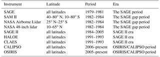
Figure 2Distribution of SAGE II observations throughout its lifetime with one dot per event. From October 1985 to July 2000, there are about 10 000 events per year. Due to an instrument fault, there are no events from August to October 2000 and the instrument operates on a half duty cycle (a mix of sunrise and sunset events) until the end of its mission in August 2005.
2.1 The “no fill” data set
The GloSSAC data set is a zonal data set in 5∘ latitude spanning 80∘ S to 80∘ N pseudo-month (1∕12 year) bins. The monthly period roughly spans the period for space-based solar occultation instruments such as SAGE and SAGE II to span the limits of their latitudinal coverage. Depending on season, details of the orbit, and observation requirements, this whole class of instruments provide data from equatorward of roughly 60∘ and require roughly a month to cover this latitude range. Similar instruments in sun-synchronous orbits, which have fixed equatorial cross times (generally preferred for nadir-viewing instruments), make measurements primarily poleward of 60∘ in both hemispheres. SAM II and POAM III are examples of instruments in this type of orbit. Figure 2 shows the measurement locations for SAGE II, the primary source of data between 1984 and 2005 that demonstrates the seasonal location of observations. From this figure, it is clear that no observations occur in the winter hemisphere poleward of 50∘ and observations at low latitudes have a much lower frequency of occurrence than measurements in midlatitudes. Given the space-based measurement latitude sampling, there really is not a “natural” latitude resolution on which to produce the data product grid. If there was an attempt to produce one, it would likely be finer in midlatitudes and broader in high- and low latitudes. A variable grid while perhaps more in-line with the observations is not a desirable format for any end-user of the data set and as such, we use a fixed grid resolution of 5∘ throughout the data set. It would be difficult to produce the analysis on a shorter timescale without relying almost solely on additional interpolation. However, it is possible that during the CALIPSO/OSIRIS era, a period significantly shorter than a month could be used, but at this point, for continuity's sake, the entire data set is produced in monthly bins.
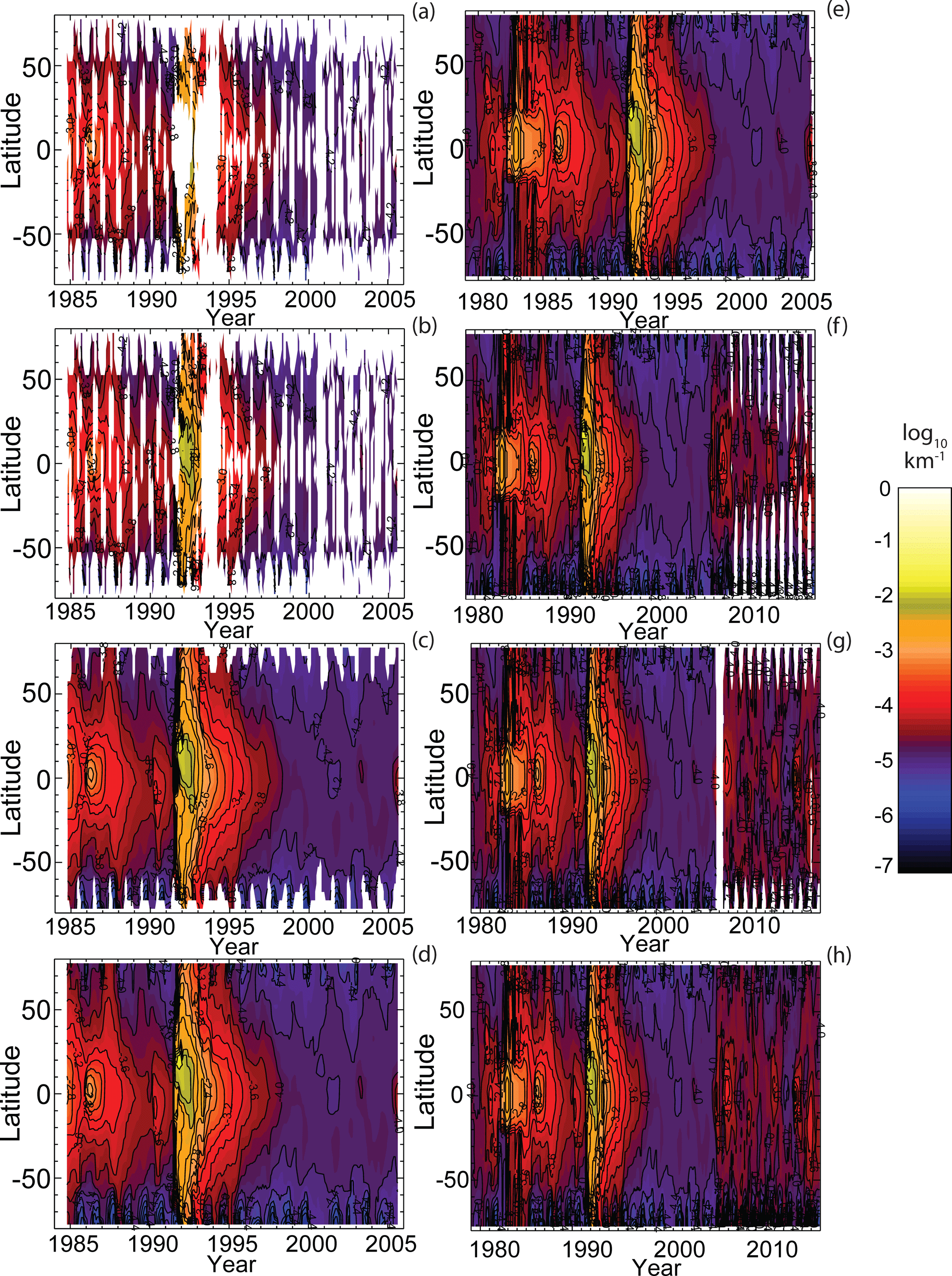
Figure 3Steps involved in the creation of the GloSSAC 1020 nm aerosol extinction coefficient climatology at 21 km: (a) 1984–2005 with SAGE II only, no interpolation; (b) with SAGE II, CLAES, HALOE, and ground based-lidar, no interpolation; (c) with interpolation; (d) with high-latitude reconstruction; (e) 1979–2005 with the pre-SAGE II era data from SAGE, SAM II, airborne and ground-based lidar; (f) 1979–2016 adding only OSIRIS; (g) 1979–2016 adding only CALIPSO; and (h) 1979–2016 adding both OSIRIS and CALIPSO and producing the final product. The plotting software tends to exaggerate white space in the plots particularly in (a) and (b).
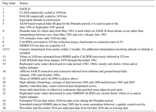
The initial step in producing GloSSAC is to produce gridded data sets for SAGE II at its four wavelengths (386, 453, 525, and 1020 nm) and HALOE and CLAES aerosol measurements at selected wavelengths. We assign each bin a flag that indicates its source and preserve both the number of data points used and the number identified as containing cloud. We show the complete set of flag values in Appendix B. The data are reported on a 0.5 km vertical grid from 5.0 to 39.5 km. This is the native SAGE II reporting resolution though its true vertical resolution is ∼ 1.0 km (Damadeo et al., 2013). This initial step in the GloSSAC development is shown in Fig. 3a for the 1020 nm extinction. Most other instruments used in this data set have a lower native vertical resolution and are interpolated to this grid. An exception is the CALIPSO backscatter coefficient data that have a vertical resolution of approximately 180 m in the lower stratosphere. However, as will be discussed later, the high measurement noise in this data set precludes reporting data at such a fine resolution. In general, differences in vertical resolution are only important in a few situations. Near the tropopause, the presence of clouds is sometimes inferred in the lower tropical stratosphere by instruments with coarse vertical resolution such as CLAES, HALOE, and OSIRIS (1.5–2.5 km) when the clouds are most likely tropospheric. There is also, generally, a strong gradient in aerosol extinction across the tropical tropopause (relatively low in the troposphere and higher in the stratosphere) that may be smeared out somewhat by a larger vertical resolution. Finally, strong vertical gradients are common in the aftermath of a volcanic injection of material into the stratosphere as the initial plume can be strongly stratified (Winker and Osborn, 1992). Broad vertical resolution tends to smear these edges out. Mixing data from instruments with different vertical resolutions during a strongly post-volcanic period can create some anomalous inferences regarding aerosol properties across edges of volcanic clouds by treating volcanic and non-volcanic observations as coincident observations. The most prominent period when this is a concern is the post Pinatubo period when SAGE II (∼ 1 km vertical resolution), CLAES, and HALOE (both with ∼ 2 km vertical resolution) are available. As a result, it is possible to have a variable degree in which the instruments capture an optically thick discrete layer. The presence of strong vertical gradients in an inference of aerosol size distribution or other parameter can be compromised and yield unpredictable and nonphysical results when using data with different vertical resolutions. Since we provide data from complete and often overlapping fields for these instruments, users need to exercise caution when using the data set in this period.
For a given latitude/month bin, we collect all aerosol extinction coefficient profiles within 5∘ of the latitude of the center of the bin (bins overlap by 2.5∘ with latitude bins to the north and south). In order to report a value, we require a minimum of five valid data points and that at least 50 % of the available profiles in that time/latitude are available at that altitude, otherwise the bin is marked as missing. We report the median value of valid points at each grid location. The monthly/latitude profile is continuous from 40 km down to at least the tropopause and often several kilometers below that level.
The processes that terminate SAGE II profiles control the lower extent of data and these vary among the four measurement wavelengths. Individual profiles are terminated by either high molecular extinction (at shorter wavelengths), optically dense clouds (all wavelengths), encountering the solid Earth (usually just for 1020 nm extinction profiles), and, during Pinatubo, very high aerosol extinction levels (all). We also exclude any observations in which we infer the presence of non-opaque clouds. We identify these clouds using the method described by Thomason and Vernier (2013) (a revision of an algorithm developed by Kent et al., 2003) and exclude those points from the analysis. We infer cloud presence almost exclusively in the troposphere; however, we occasionally infer the presence of clouds in the lower tropical stratosphere. In addition, we are able to detect and exclude ice polar stratospheric clouds (PSCs) but it is likely that saturated ternary solution (STS) and nitric acid trihydrate (NAT) PSCs slip by the cloud identification process. This occurs because the methodology relies on the dominating presence of “large” aerosol particles that are mostly lacking for these types of PSCs. Away from Pinatubo, 525 and 1020 nm extinction coefficients are available throughout the stratosphere. Profiles at 453 and 386 nm are available down to about 12 and 16 km, respectively. It should be noted that the aerosol data at 386 nm are biased low below 20 km and above the main aerosol layer and are at best of limited quality under all conditions and altitudes. Following Thomason et al. (2010), while the data are included in the data set, we recommend caution using SAGE II 386 nm data. Finally, we exclude any data below the highest altitude at which 1020 nm aerosol extinction coefficient exceeds 0.01 km−1 because of potential artifacts in SAGE II data at altitudes where the atmosphere is essentially opaque.
Both CLAES and HALOE flew aboard the Upper Atmosphere Research Satellite (UARS) and all UARS data are reported at pressure levels rather than altitude like SAGE II. Median-based extinction profiles on the native pressure grid are derived following rules similar to those used with SAGE II (profiles are terminated at the bottom if less than 5 data points are available or less than 50 % of the available profiles in that time/latitude are available at that altitude). We interpolate the profiles to the standard altitude grid using altitude-log pressure from the Modern-Era Retrospective Analysis for Research and Applications (MERRA; Rienecker et al., 2011) data that is used in SAGE II data processing. CLAES (October 1991 to April 1993) aerosol extinction data are used at 1257 cm−1 (7.8 µm) and 780 cm−1 (12.8 µm). While the information content from an aerosol perspective is essentially identical for these two channels, the wavelength dependence changes between sulfate aerosol and ice clouds and so changes in this ratio are used to identify measurements that are influenced by ice clouds and those measurements are excluded from further analysis. CLAES extinction coefficient data, while well behaved, have a bias between the channels and compared to other measurements (Massie et al., 1996), and it is difficult to determine based on physical arguments where the cut off between sulfate aerosol and ice clouds should occur. As a result, we use an empirical outlier approach in which the presence of cloud is identified when aerosol extinction at 1257 cm−1 is greater than 10−3 km−1 and the 780 to 1257 cm−1 extinction coefficient ratio is significantly larger than generally observed bounds as shown in Fig. 4. The points identified in this manner uniformly lie in the upper troposphere/lower stratosphere most often at lower latitudes and suggest influence by tropospheric clouds. When applied, this process removes what appear to be cloud artifacts without appreciably affecting the remainder of the analysis.
We use HALOE (October 1991 to 2005) data at 3.40 µm following the findings of Thomason (2012) and correct for NO2 absorption following the recommendations in that paper. This is based on the idea that sulfate aerosol extinction at 3.40 and 3.46 µm should be essentially identical (< 1 % differences). However, we observed particularly at low extinction that the extinction at 3.40 µm is usually greater than that at 3.46 µm. This difference correlates well with NO2 for which the 3.40 mm aerosol extinction coefficient product is not corrected in routine HALOE processing. Nominally, the aerosol at 3.46 µm is useful as reported above 20 km but not below that altitude, whereas 3.40 µm data are useful to the tropopause except for the NO2 artifact. To correct the 3.40 µm aerosol data, we use an empirical relationship between HALOE observations of NO2 and the difference between 3.40 and 3.46 µm aerosol extinction coefficient values where all three values are available and considered robust. This difference is applied to the 3.40 µm data wherever it and the HALOE NO2 molecular number density are available (generally down to about 15 km). The existence of HALOE NO2 observations is the limiting factor determining the lowest altitude for which HALOE aerosol data are usable. Only the corrected 3.40 µm aerosol extinction coefficient data are archived as a part of the data set. Figure 5 shows the relationship derived for the NO2 correction; the aerosol extinction coefficient correction can be as much as 10 %. There is no cloud clearing necessary for the HALOE data set since the corrected data are not available near or below the tropopause nor are they used within the winter polar vortex that would require clearing of PSCs.
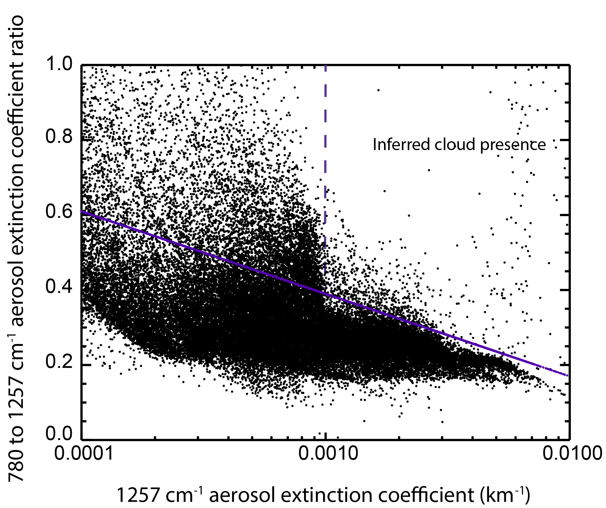
Figure 4The distribution of CLAES 780 to 1257 cm−1 aerosol extinction coefficient measurements as a function of 1257 cm−1 aerosol extinction coefficient. Areas about and to the right of the blue lines almost exclusively occur in the lower stratosphere and appear to be associated with the presence of clouds. These points are excluded from further analysis.
2.2 Filling gaps in the SAGE II data set: alternative data sets
One of the goals of GloSSAC is to have a continuous “gap-free” data set for 1979 through 2016 at both 525 and 1020 nm. The former is comparable to other long-term data sets like the GISS stratospheric aerosol optical depth record, while the latter is the most robust aerosol measurement available from the SAM/SAGE series and available wavelength for most of the “SAGE” era from 1979 to 2005. However, there are important gaps in the lower stratosphere from the eruption of Pinatubo in June 1991 well into 1993. In addition, a number of SAGE II profiles are compromised by short duration events. These events mostly occur in 1993 and are primarily sunrise events where measurement-taking was terminated before sufficient exoatmospheric data were taken for robust normalization to transmission. The events were temporarily shortened during a period in which the spacecraft batteries were rapidly degrading. Event durations were returned to their normal length in early 1994. As a result, complete 525 and 1020 nm records require the use of non-SAGE II data during this period.
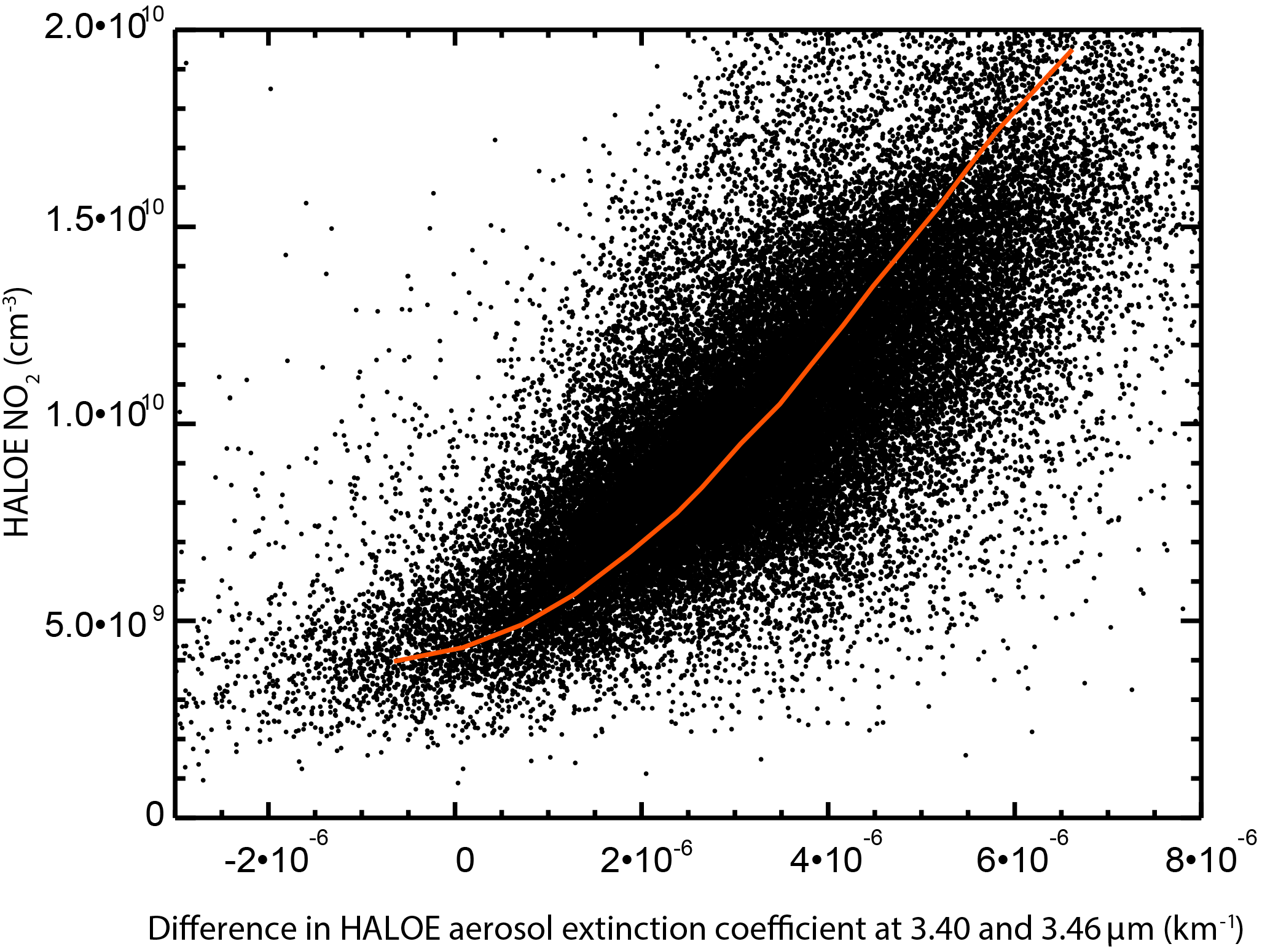
Figure 5All HALOE NO2 between 20 and 30 km plotted against the corresponding difference between HALOE aerosol extinction coefficient measured at 3.40 and 3.46 µm.
Following the general GloSSAC data use paradigm, while other data sets are available, CLAES and HALOE are shown below to be reasonably well-behaved and sufficient for the filling process. CLAES and HALOE data offer similar near-global coverage through most of this period (October 1991 and onwards) if the data can be transferred from the measurement wavelengths to SAGE II wavelengths in a robust manner. Figures 6 and 7 show the observed relationship between SAGE II extinction coefficient measurements and CLAES at 1257 cm−1 and the corrected HALOE data at 3.40 µm. In general, CLAES data are well correlated with SAGE II measurements. HALOE measurements are not as well correlated and, as a result, only used where neither SAGE II nor CLAES data are available. On the one hand, Thomason (2012) showed that HALOE and SAGE II during high to moderately volcanic periods generally follow expectations for sulfate aerosol distributed in submicron aerosol size ranges. On the other hand, Massie et al. (1995) argued that CLAES and SAGE II are biased relative to expectations by a factor of approximately 2 since it is difficult to imagine a sensible aerosol size distribution and composition that would produce the observed relationship. As a result, given the desire to avoid discontinuities within the data set, we use an empirical relationship between SAGE II at 1020 nm and both HALOE (corrected 3.40 µm) and CLAES (1257 cm−1) aerosol data to produce aerosol extinction at 1020 nm. We also produce a corresponding value of 525 nm aerosol extinction coefficient using the relationship observed between SAGE II at 1020 and 525 nm. We show the 525 to 1020 nm extinction coefficient relationship in Fig. 8. There are issues with the use of this relationship outside the SAGE II period that we discuss in detail below. The empirically derived data are placed in the 1020 and 525 nm aerosol extinction coefficient grid only where SAGE II data are missing because of a lack of measurements at a given latitude or the result of the loss of data due to the opacity of the Pinatubo volcanic aerosol layer. Since HALOE data are most robust at higher aerosol levels, we use them only between the start of its mission in October 1991 and the end of 1993 and only to fill altitudes in the lower stratosphere where both SAGE II and CLAES data are missing.
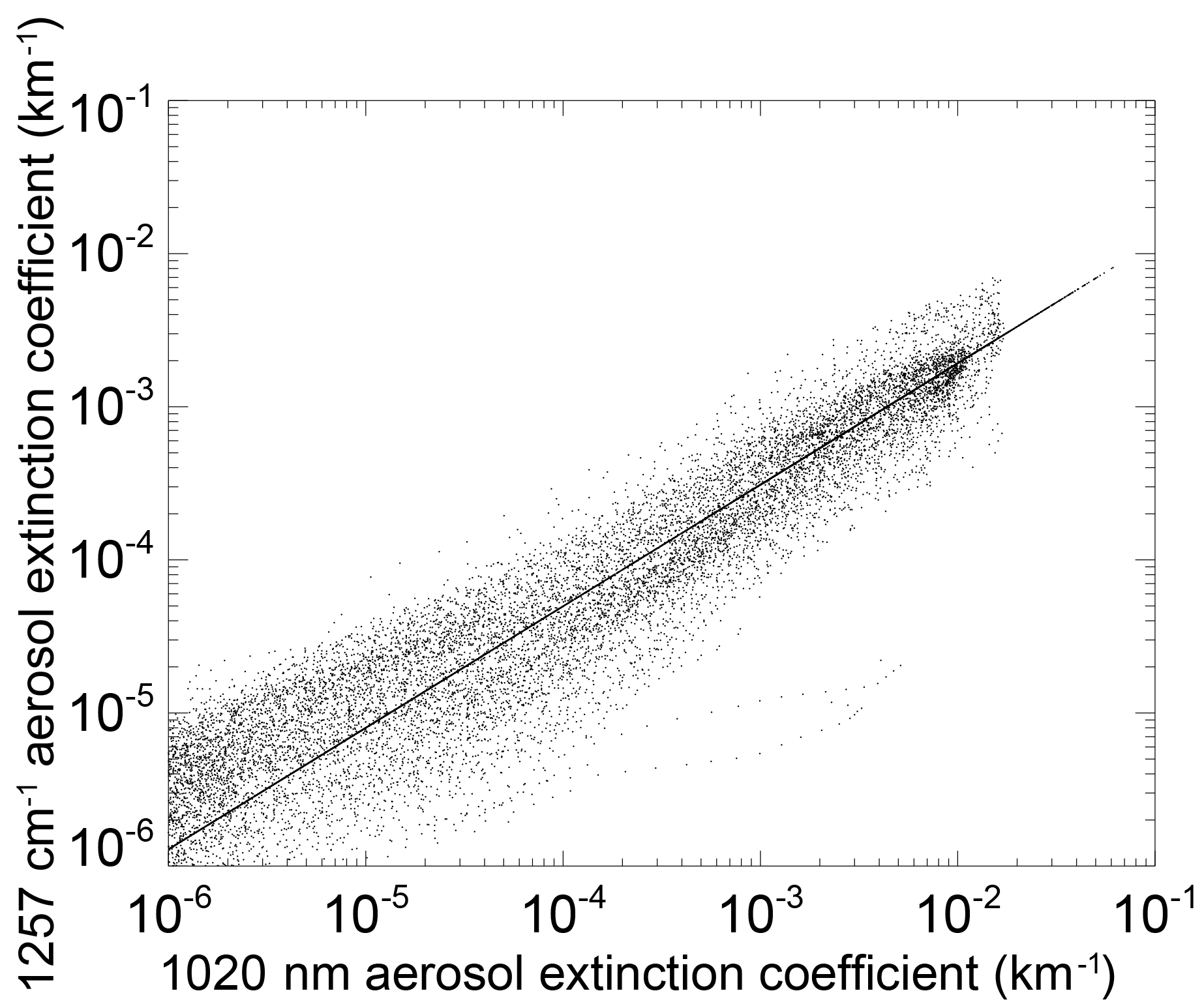
Figure 6Relationship between the gridded and cloud-cleared CLAES 1257 cm−1 aerosol extinction coefficient versus SAGE II gridded and cloud-cleared 1020 nm aerosol extinction coefficient. The solid line shows the conversion relationship used for converting CLAES to SAGE II 1020 nm extinction coefficient.

Figure 7Relationship between corrected HALOE 3.40 µm aerosol extinction coefficient and the observed gridded and cloud-cleared SAGE II observations at 1020 nm. The solid line is the empirical conversion used to infer 1020 nm aerosol extinction coefficient from HALOE observations at 3.40 µm.
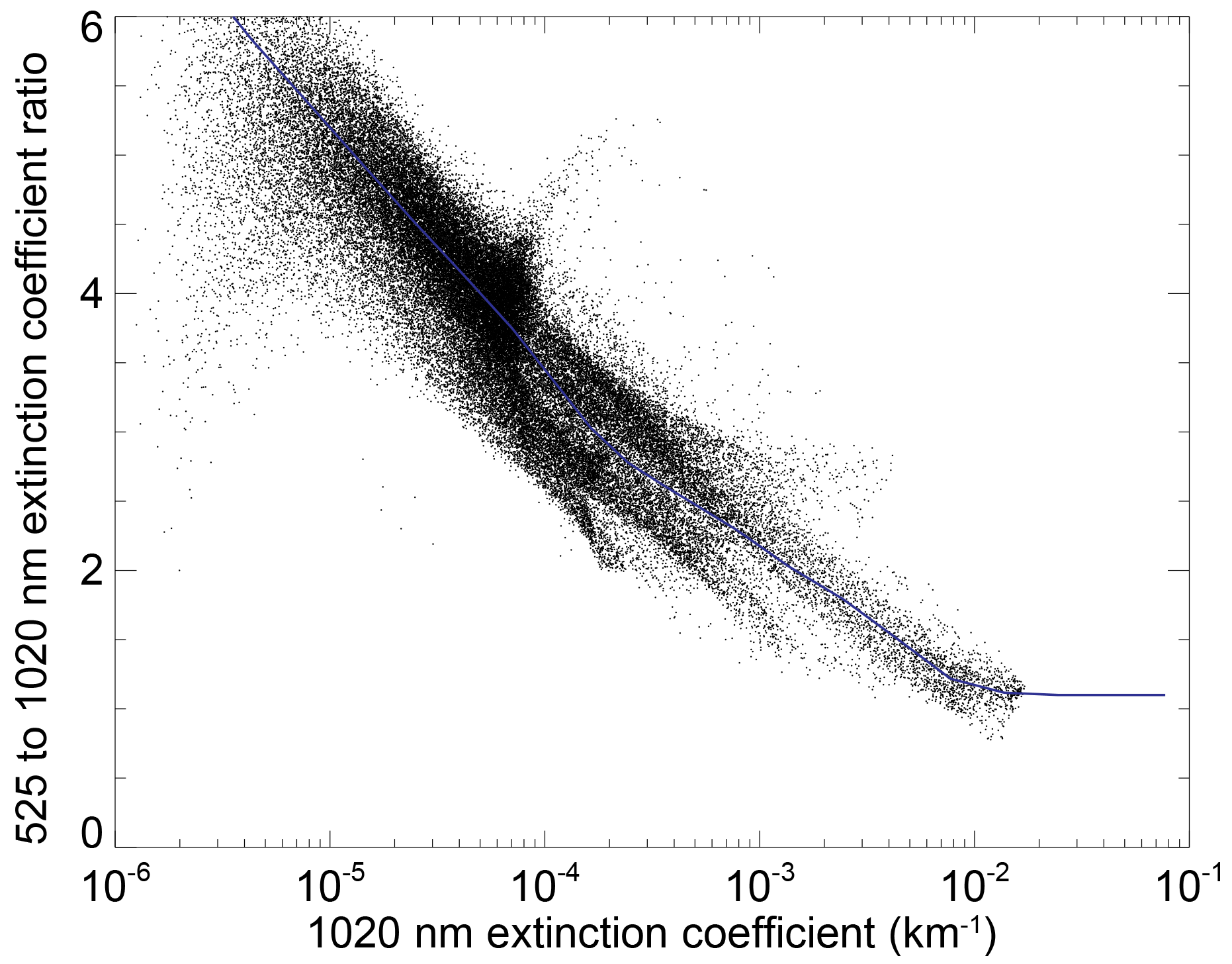
Figure 8Observed relationship between gridded and cloud-cleared SAGE II observations (below 30 km) as a function of SAGE II 1020 nm observations. The blue line is the conversion relationship used for 1020–525 aerosol extinction conversion throughout GloSSAC development.
The summer of 1991 presents special problems for the reconstruction while at the same time being a crucial period for the evaluation of the performance of chemistry-climate models. SAGE II data are missing at altitudes as high as 25 km after the eruption and UARS data are only available starting in October. An additional issue for this period is that there are no SAGE II observations (and no truly tropical data at all) in June 1991. In previous versions, SAGE II data were interpolated between May and July 1991 producing values with no observational basis in this month. For GloSSAC, we have replicated the missing data between 20∘ S and 20∘ N using data only from May 1991 so that only minor enhancements from the Pinatubo eruption appear in June 1991 and only poleward of 20∘ N. The massive enhancements in tropical aerosol levels do not appear in the GloSSAC data set until July 1991. For those who wish an enhancement at the time of the eruption, averaging GloSSAC for May 1991 and July 1991 data will produce a June 1991 analysis similar to that provided in early data sets. Another solution for users is to use GloSSAC data for May 1991 for May and June through the 14th and use data for July 1991 from 15 June (the date of the largest eruption) through July. Neither approach yields a fully satisfactory representation of the complexity of the initial volcanic aerosol distribution observed immediately after the eruption.
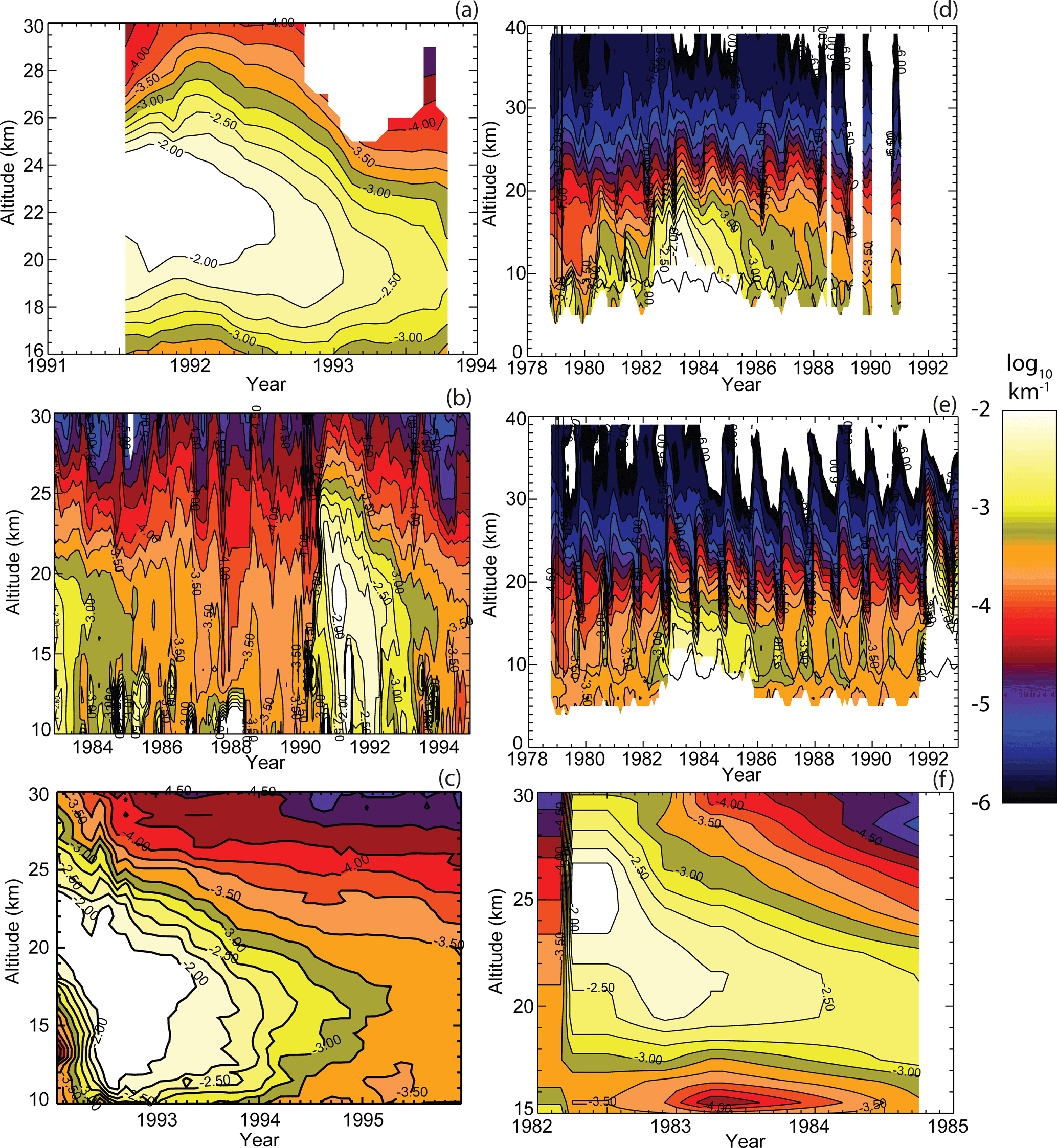
Figure 9Component contributors to GloSSAC or previous versions all shown in aerosol extinction coefficient at 1020 nm. They include: (a) the ASAP-based Camaguey–Mauna Loa “tropical” construction, (b) NASA LaRC 48-inch lidar record, (c) NIWA Lauder backscatter sonde Pinatubo record, (d) SAM II Southern Hemisphere, (e) SAM II Northern Hemisphere, and (f) the ASAP-derived airborne lidar/SAGE/SAGE II tropical reconstruction for 1982 to 1984.
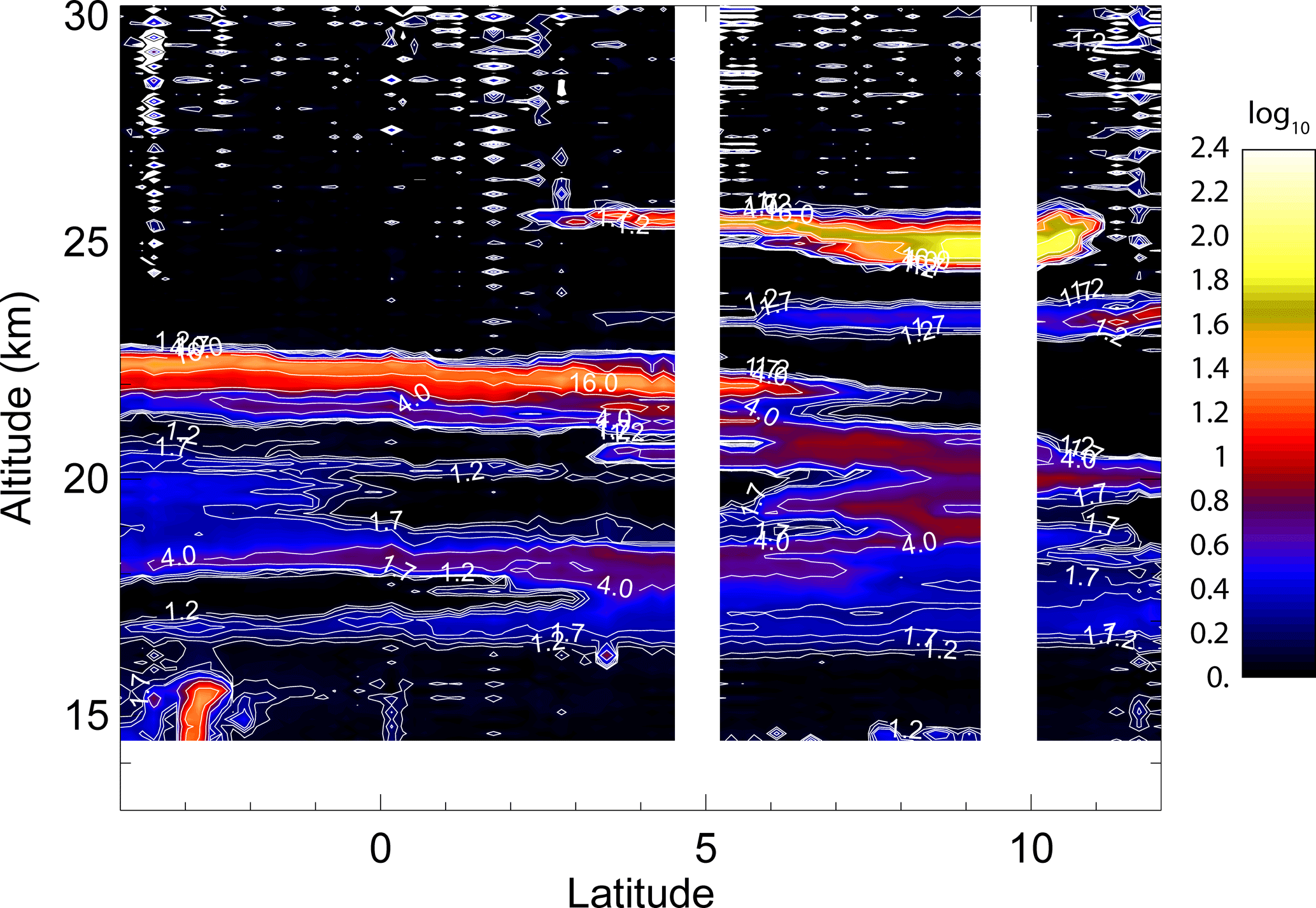
Figure 10Aerosol backscatter ratio from the July 1991 airborne lidar mission aboard the NASA DC-8. Contours are at 1.2 (dark blue), 1.4, 1.7, 2, 4, 8, 16, 32, 64 (orange) with a highest observed value at 82 (yellow). Above 17 km, all of the contours are associated with relatively fresh Pinatubo aerosol.
For July to September 1991, we make use of the tropical reconstruction created for the ASAP analysis, which is a combination of data from the lidar station operated by the Centro Meteorológico de Camagüey in Cuba (23∘ N) lidar data set (Antuña, 1996) and the NOAA ESRL lidar at Mauna Loa (19∘ N; Barnes and Hofmann, 1997). It is likely that neither station's data are representative of the equatorial aerosol levels following the Pinatubo eruption and are more likely to be too small than too large. Therefore, rather than averaging the two time histories, we used the maximum value observed during the month with the hope of reproducing the tropical enhancement using data from two subtropical sites. The reconstruction is shown in Fig. 9a. In ASAP Fig. 4.32, the reconstruction is shown to do a reasonable job of reproducing the SAGE II-observed tropical data in that summer (mostly above 23 km) and onwards, but it should be recognized that the potential for substantial error exists during this period. For the summer of 1991, we use SAGE II where it is available in the tropics (following standard gridding rules) and we use the ASAP lidar reconstruction where it is not. We weigh the lidar values in August (0.33/0.67) and September (0.67/0.33) with the CLAES/SAGE II October values to smooth across an otherwise discontinuous step. Users of GloSSAC should recognize that no monthly gridded product can do justice to the complexity of the initial development of the Pinatubo aerosol cloud. The cloud was highly stratified and spatially inhomogeneous throughout the summer of 1991. An airborne mission aboard the NASA DC-8 in mid-July 1991 included a lidar system that captured a view of this inhomogeneity. In Fig. 10, lidar backscatter ratio data from 12 July shows the aerosol cloud along a transit through the Caribbean that has multiple optically dense layers with backscatter ratios up to 80. For comparison, prior to the eruption the entire stratosphere had aerosol ratios less the 1.2, the smallest contour level on this plot.
With the addition of CLAES observations, midlatitudes no longer need patching by non-space-based data sources as in previous versions since there is little or no loss of data in mid- and high latitudes between the eruption of Pinatubo and the start of the CLAES mission. In previous versions, the primary method to fill missing data in the mid- and high-latitude lower stratosphere between June 1991 and mid-1993 were data from the NASA Langley 48-inch lidar facility (Osborn et al., 1995) and data from the University of Wyoming backscatter sonde (Rosen and Kjome, 1991; Rosen et al., 1997) deployed from the NIWA Lauder (New Zealand) facility. We show these data sets in Fig. 9b and c. Recently, we have recovered and archived data from NASA Langley airborne missions in July 1991 and May 1992 at the NASA Atmospheric Sciences Data Center,2 which may provide corroborative data to future versions. The addition of the CLAES, HALOE, and lidar data sets to the GloSSAC analysis is shown in Fig. 3b.
2.3 Filling the gaps: interpolation
At this point, there are still substantial gaps throughout the data set, mostly because of the spatial sampling pattern of a mid-inclination solar occultation instrument. Gaps are filled using linear interpolation in time but not in altitude or latitude. While we could interpolate and completely fill the grid, in practice, interpolation is limited to gaps of no more than 2 consecutive months. This works well in mid- and low latitudes except in late 2000 where SAGE II was off for several months due to an instrument error. In this case alone, interpolation is permitted to 4 months since it is a relatively benign period and there are few data available to provide alternative guidance. We do not believe that this seriously compromises the analysis. The most significant issue in this period is a poor depiction of the Antarctic polar vortex in austral spring, where it is effectively missing entirely. With the allowable degree of interpolation, the GloSSAC 1020 nm grid at 21 km is now filled except at high latitudes in winter as shown in Fig. 3c.
2.4 Filling the gaps: high latitudes
At high latitudes, the 2-month requirement leaves substantial gaps in the winter hemisphere at latitudes as low as 60∘. In the past (ASAP, CCMI), the temporal window was simply expanded and interpolations across gaps as large as 6 months were permitted. However, the winter poles are generally low (relative to midlatitudes) in aerosol (in the absence of PSCs) due to their isolation from midlatitudes and the diabatic subsidence within the polar vortex (Kent et al., 1985). As a result, the polar vortex, particularly in the Northern Hemisphere where SAGE II sampling is strongly affected by temporal/spatial sampling, is poorly represented in these earlier data sets. For GloSSAC, we have developed an alternative approach based on the observation that while there are large gaps in the analysis in latitude space, it is almost completely filled in equivalent latitude space thanks in part to the meridional asymmetry in the polar vortex commonly observed in both hemispheres as shown by Manney et al. (2007) and references therein. Figure 11a shows the aerosol extinction coefficient at 1020 nm and 21 km for the SAGE II lifetime as a function of time and latitude.3 We reconstruct the aerosol fields where data are missing in latitude space from those in equivalent latitude using the relationship
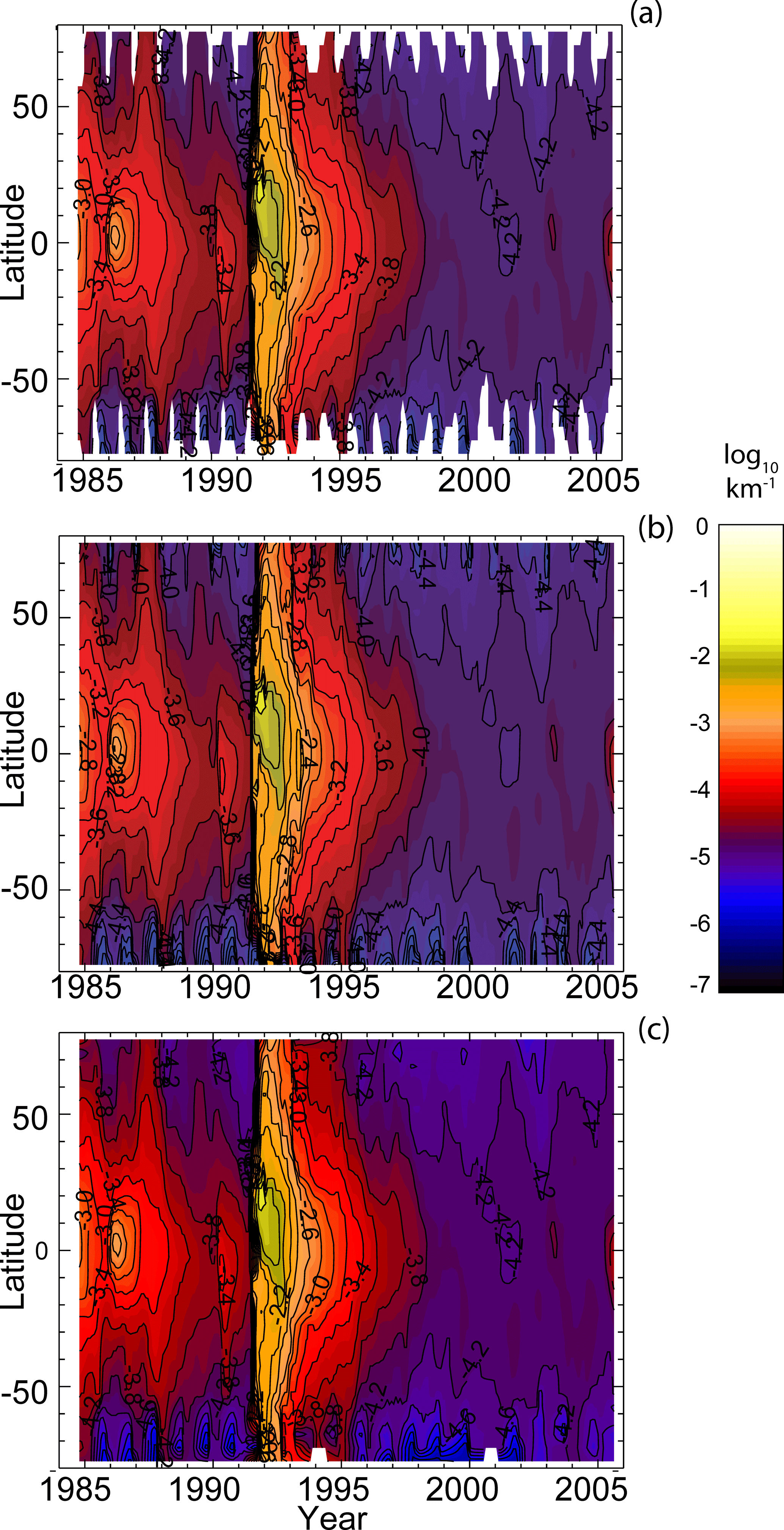
Figure 11GloSSAC analysis prior to using the equivalent latitude filling process (a) and afterwards (b). (c) Shows the use of brute temporal interpolation to fill high latitudes.
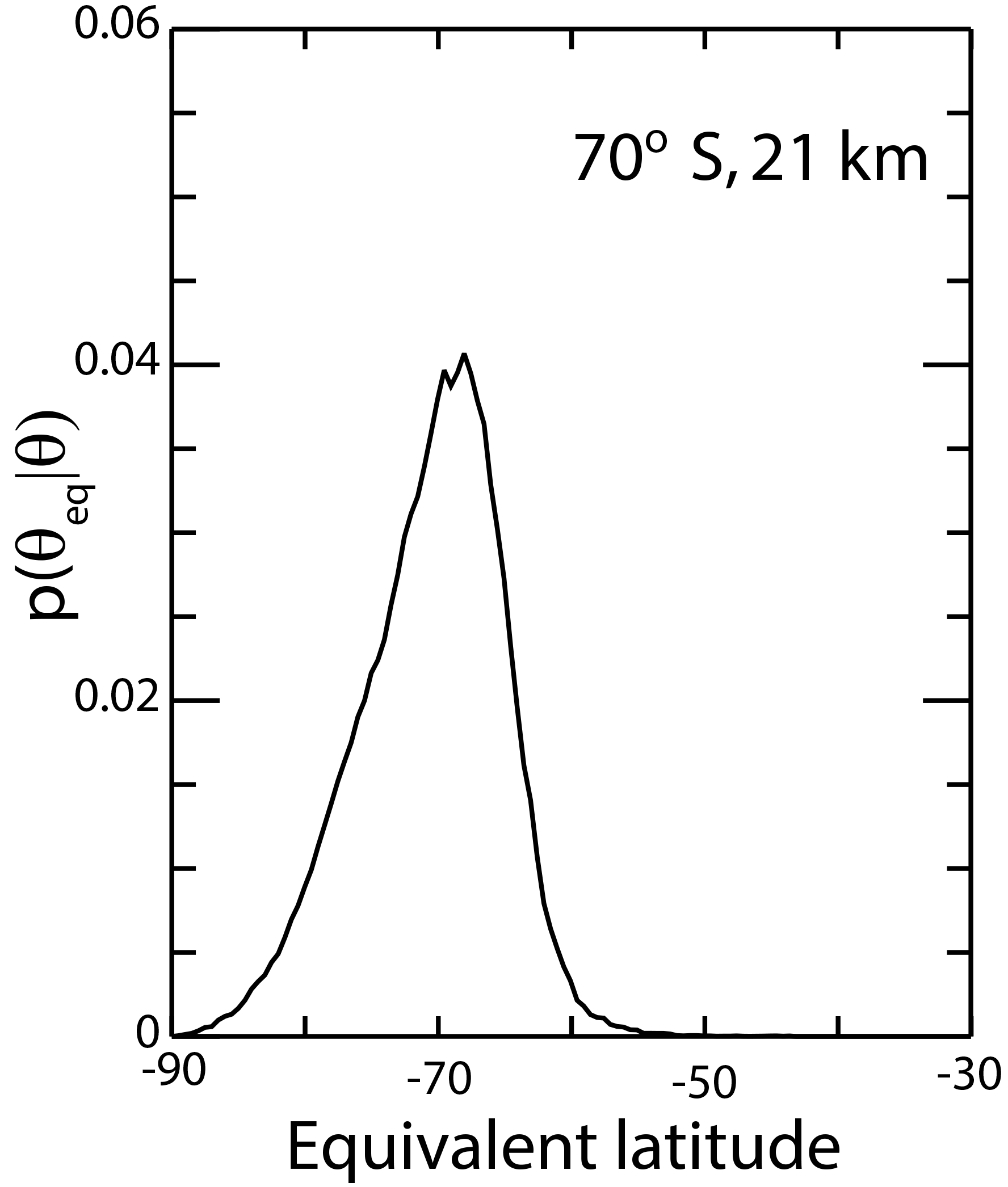
Figure 12Distribution of equivalent latitude (per degree) for August at 70∘ S and 21 km based on a 10-year average of MERRA observations for 2001 to 2010.
where kλ is extinction coefficient at wavelength λ at latitude/equivalent latitude θ or θeq at altitude z and time (month) t. The function p is the distribution of equivalent latitude in bins “n” at a given latitude. Using this approach, we can estimate extinction at latitudes not directly observed by SAGE II. The approach is analogous to the potential vorticity reconstruction process introduced by (Schoeberl et al., 1989; Manney et al., 1999, 2001, 2007; Randall et al., 2005), though in this case we are only interested in reconstructing the zonal mean. It assumes that the distribution of aerosol extinction coefficient at all levels is correlated with equivalent latitude. Averaging by latitude tends to smear out the vortex boundary compared to an equivalent latitude analysis (Manney et al., 1999, 2001) and thus increase the zonal standard deviation of the aerosol extinction coefficients. In practice, we find that the zonal variance in equivalent latitude space is about equal to or somewhat less than that observed in latitude space. This is particularly true near the vortex boundary where the reduction in zonal standard deviation is as much as one-third. The function p is derived from MERRA analyses for 2000 through 2010. An example of these distributions is shown in Fig. 12. Figure 11b (and Fig. 3d) shows an example of the reconstructed latitude analysis (20 km), while Fig. 11c shows the “brute force” interpolation across the wintertime gap (consistent with the analysis provided to CMIP5/CCMI). It is clear that the clean polar vortex is captured far more clearly, particularly in the Northern Hemisphere, in the reconstructed data. Considering that the scale of the vortex/extravortex differences, particularly in volcanic periods, can be as large as a factor of 10, the new approach of filling high latitudes is a vast improvement relative to previous versions.
3.1 The SAGE period (January 1979 to November 1981)
During the SAGE lifetime (January 1979 to November 1981), the 1000 nm aerosol extinction coefficient measurements form the basis of the overall analysis. We did not use the SAGE 450 nm measurements in this analysis since they are poor quality and not usable at all below 20 km (Thomason et al., 1997a). The SAGE data are supplemented by 1000 nm extinction measurements by the Stratospheric Aerosol Measurement (SAM II; 1978–1993), which provide data only at high latitudes (> 60∘). This data set enabled some of the earliest observations of PSC and a PSC climatology that remains valuable (Poole and Pitts, 1994). We do not use SAM II during the SAGE II period because comparisons with SAGE II suggest that SAM II is biased low by as much as 30 %. However, with the dearth of data in the 1979 to 1984 period, we had essentially no choice but to use these data. We have used only SAM II data that we identified as occurring outside the polar vortices similar to the procedure used by Bevilacqua et al. (1997). Unfortunately, this precludes capturing the clean wintertime vortex throughout this period. We made this decision since we were unable to adequately clear PSCs from the SAM II data and, rather than a clean vortex, a substantial enhancement in the winter hemisphere would result. The SAGE team expects to produce a new version of SAM II data in the near future and we will then reconsider the role of SAM II in future versions of GloSSAC. We create the data record up to the end of the SAGE mission in November 1981 using SAGE and SAM II 1000 nm data and the sampling and interpolation method described for the SAGE II period with no additional steps. Throughout the pre-SAGE period, we produce the data at 1020 nm and then infer the magnitude at 525 nm using the relationship from SAGE II shown in Fig. 8.
3.2 The SAGE gap period (December 1981 to September 1984)
The SAGE “gap” period from December 1981 to September 1984 is of critical interest since it encompasses the El Chichón eruption (March/April 1982). However, with very limited space-based measurements available4 and rather limited data of any sort, the analysis for the period from December 1981 to September 1984 is challenging. While additional data sets are available in this period, we follow the GloSSAC data use paradigm to use a few long-lived data sets and those with a unique spatial context such as the tropics. We follow the method described in ASAP (2006) with only minor changes to the process. To reconstruct the aerosol fields in this period, we have used the last full month of SAGE data (November 1981) for December through March 1982, which effectively preserves a fairly clean stratosphere up to the El Chichón eruption which occurred in late March. Beginning in April 1982 until the beginning of SAGE II observations in 1984, we used a composite of data consisting of SAM II, the NASA Langley 48-inch lidar system, lidar data from the NASA Langley Airborne Lidar System, and the October 1984 SAGE II data at 1020 nm to produce the monthly grids. This uses nearly all available long-term data sets available during this period.
In the Northern Hemisphere, the 1000 nm extinction record is filled with SAM II (shown in Fig. 9d and e) between 80 and 65∘ N. From 65 to 40∘ N, we have used a linear interpolation in latitude of the logarithm of extinction between the SAM II data and 1000 nm aerosol extinction derived from the NASA Langley 48-inch lidar system. From 40 to 25∘ N, the lidar 1000 nm data are used (shown in Fig. 9b). The lidar, in this period, operated at 694 nm (ruby) and measurements are converted to 1020 nm extinction using a value for extinction to backscatter ratio of 30 sr. This value gives reasonable agreement with SAM II extinction measurements (see below) and lies within reasonably accepted bounds for this value (Thomason and Osborn, 1992; Jager and Hofmann, 1991). Latitude bins between 25 and 80∘ S are filled using Southern Hemisphere SAM II data shifted in altitude as a function of latitude following zonally averaged potential temperature surfaces. We report data throughout the pre-SAGE II period down to the altitude bin containing a climatological mean tropopause height derived from MERRA data in the SAGE II era (this data set is contained in GloSSAC) and flaged as missing all data below this level.
At low latitudes and southern midlatitudes, virtually no data are available except from airborne lidar missions conducted by NASA between 1982 and 1984. Five airborne lidar missions were flown in July 1982 (13 to 40∘ N), October–November 1982 (45∘ S to 44∘ N), January–February 1983 (28 to 80∘ N), May 1983 (59∘ S to 70∘ N), and January 1984 (40 to 68∘ N).5 These data are also made at 694 nm and converted to 1020 nm extinction coefficient using an extinction to backscatter ratio of 30 sr. For April through July, the southernmost (13∘ N) airborne lidar profile from July 1982 is used. Following that period, we use a linear interpolation in time of the logarithm of 1000 nm aerosol extinction estimated from lidar profiles in July 1982, October 1982, May 1983, and the SAGE II tropical data in October 1984. The reconstruction is shown in Fig. 9f. We use the tropical reconstruction 10∘ S and 10∘ N and then interpolate with the mid-latitude data (SAM II in the south and 48-inch lidar in the north) between 10 and 25∘ in both hemispheres. Latitude bands where we employ the various data sets are set based upon where we believe, based on experience, they are most applicable. However, it is clear that this part of the construction is data sparse and we are compelled to use the available data in ways we would not in more data-rich periods. It is likely that unexploited sources of data exist and further study and perhaps historical data recovery efforts in this period would be worthwhile.
After the end of the SAGE II mission in August 2005, the stratospheric aerosol extinction coefficient climatology becomes solely dependent on aerosol measured by OSIRIS and CALIPSO. This represents not only a change in instrument but also the way in which aerosol is measured. OSIRIS measures limb scatter radiance from which aerosol extinction coefficients at 750 nm (and other parameters) are inferred. CALIOP is the CALIPSO platform's nadir-viewing lidar that produces a stratospheric backscatter aerosol coefficient product primarily at 532 nm. While these changes represent some challenges to the continuity of the overall climatology, they both produce near-global coverage on a daily basis. Though we have not exploited the potential for higher temporal resolution for GloSSAC v1.0, we are considering how to exploit the higher temporal resolution data for future versions.
4.1 OSIRIS
For GloSSAC, we used the OSIRIS aerosol extinction climatology as produced in (Rieger et al., 2015). This climatology provides monthly latitude- and altitude-resolved extinction converted to 525 nm and bias corrected to SAGE II. Although this climatology removes much of the bias between the two instruments, the methods used in Rieger et al. (2015) are slightly different than those used to create the SAGE II climatologies in this paper. For instance, the latitude bins are 5∘ wide rather than 10∘; therefore, the OSIRIS extinction data require some amount of further correction as described below. In future versions, we will adopt a more consistent approach to construction of the underlying climatologies.
4.2 CALIPSO
The primary issues associated with the use of backscatter data from CALIPSO are measurement calibration and noise. The noise can be reduced by averaging millions of profiles to obtain zonally averaged data in the stratosphere on a monthly basis. Rogers et al. (2011) showed that aircraft high spectral resolution lidar measurements and CALIOP data agreed within 2.7 % ± 2.1 % at midlatitudes. However, comparison between in situ balloon-borne backscatter data and CALIOP in the tropics suggest that the normalization level where purely molecular signal is assumed should be moved from 30–34 to 36–39 km (Vernier et al., 2009). For GloSSAC, we use CALIOP version 4 level 1 data where, unlike earlier versions, the backscatter signal is calibrated at the higher altitude range. We anticipate that the residual calibration error from aerosol presence at those altitudes to be about 2 %. Due to the details of the calibration process, we expect that the total relative error on the CALIOP scattering ratio to be around 5 % (between 50∘ S and 50∘ N). In order to derive extinction profiles from CALIOP backscatter data, a lidar ratio for stratospheric aerosol needs to be assumed. This ratio can vary between 30 and 60 sr in the stratosphere (Jäger et al., 1995) and represents the major source of uncertainty when converting backscatter into extinction. On a profile-by-profile basis, CALIPSO data are substantially noisier than any other data set used in GloSSAC. However, we find that the reduction from the 1 km horizontal resolution and 60 m vertical resolution to the GloSSAC resolution generally produces data with a roughly comparable level of noise as the other data sets.
We initially calculate mean total attenuated backscatter at 532 nm every 1∘ along each CALIPSO orbit track and correct for attenuation by ozone absorption and molecular scattering using data from the Goddard Earth Observing System Model Version 5. The presence of cloud is inferred whenever at least 3 of 5 consecutive data points in a profile have depolarization ratio values greater than 5 % below 20 km. All data at and below the detection of clouds is excluded (“cleared”) from further consideration. We eliminate data below clouds due to uncorrected cloud attenuation effects on the reported backscatter data. In polar winters, some enhancement of backscatter is nearly ubiquitous in much of the polar vortex due to the take up of nitric acid into the sulfate aerosol (e.g., STS). To maintain the data set as close to a purely aerosol characterization as possible, we eliminate all CALIPSO observations when the observed temperature is less than the NAT formation temperature plus 2 K. Following these steps, we further reduce the cloud-cleared data to the GloSSAC monthly 0.5 km by 5∘ of latitude resolution.
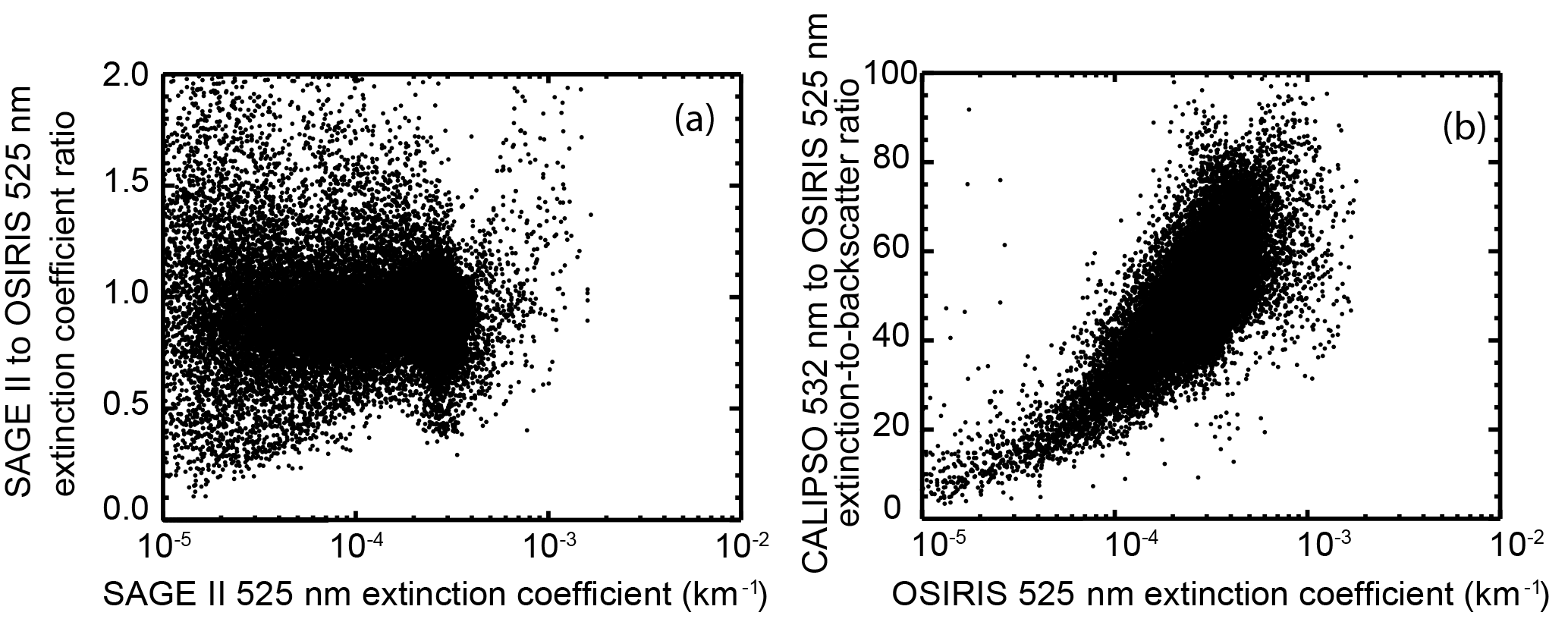
Figure 13(a) Scatter plots of observations that show the SAGE II to OSIRIS 525 nm aerosol extinction coefficient ratio where both exist in the GloSSAC data set. The average value is about 0.88. (b) Scatter plots of observations that show the CALIPSO 532 nm aerosol backscatter coefficient to the scaled OSIRIS 525 nm aerosol extinction coefficient ratio where both exist in the GloSSAC data set. The average value is about 53 sr.
4.3 Incorporating OSIRIS and CALIPSO into GloSSAC
We are fortunate to have roughly 4 years of overlap in the data from OSIRIS and SAGE II. This period is critical for understanding not only how OSIRIS and CALIPSO interrelate but also to use OSIRIS to infer indirectly how SAGE II relates to CALIPSO. Since clouds in the upper troposphere may have a deleterious impact on the measurement of aerosol extinction in the lower stratosphere (characteristic of limb measurements in general), we exclude all OSIRIS data in the lowest 2 km of the stratosphere. For the overlap period, we show, in Fig. 13a, the relationship between OSIRIS inferred 525 nm aerosol extinction coefficient and SAGE II measurements at that wavelength. Overall, the comparison is favorable; SAGE II and OSIRIS are well correlated with OSIRIS tending to be 10 to 20 % less than SAGE II (median 0.88) in a period that has the lowest aerosol loading observed between 1979 and 2016. If we use OSIRIS “as is” or scaled by the median ratio value between OSIRIS and SAGE II data sets, we observe a discontinuity at the August 2005 (SAGE II) and September 2005 (OSIRIS) boundaries. While in retrospect it may not have been the most satisfactory solution, we scaled OSIRIS to minimize an obvious discontinuity using a factor of 0.8. The switch from SAGE II to OSIRIS occurs a few months following the eruption of Manam (January 2005) that effectively signaled the end of the volcanically quiescent period that began in the late 1990s. The degree to which this event creates the discontinuity is not clear and further work on melding the SAGE II and OSIRIS records is necessary. Since OSIRIS is the only source of space-based observations between September 2005 and April 2006 we use it alone through this period. Some interpolation at mid- and high latitudes is required and we follow the interpolation method used for SAGE II observations to fill these gaps. In addition, the 2 km exclusion in the lower stratosphere leaves gaps that are only partly filled by temporal interpolation. Where bins remain unfilled, the lowest measured value in a latitude/time column is replicated down to the tropopause. This is rare and rarely for more than 1 or 2 altitude bins. As with the other periods, data in the OSIRIS-only period are flagged to indicate how we derived the value at each grid point.
It is particularly disappointing that SAGE II and CALIPSO data sets do not overlap. CALIPSO observations are always at the lower end of aerosol loading observed during the SAGE II lifetime. Fortunately, the OSIRIS/SAGE II overlap period is also primarily at low aerosol loading and permit the use of OSIRIS as a transfer medium for understanding the CALIPSO backscatter to SAGE-II-like extinction coefficient conversion. We show the ratio of CALIPSO 532 nm backscatter coefficient to scaled OSIRIS 525 nm extinction coefficient as a function of OSIRIS extinction in Fig. 13b. Nominally, we might expect some dependence on the ratio to extinction value due to a correlation between extinction magnitude and aerosol size. In fact, we do see a tail towards lower extinction-to-backscatter ratio with lower extinction values but the vast bulk of the data exists in an amorphous blob and the confidence in the observed relationship is low. Part of the lack of confidence is due to the relatively high noise exhibited by the CALIPSO data relative to the other instruments and the potential for bias associated with the normalization process used for all lidar instruments. As a result, we use the median value of this distribution (53 sr) as the sole extinction to backscatter ratio conversion factor. This value is well within expected values for extinction-to-backscatter ratio (roughly between 30 and 60 sr) and effectively maps CALIPSO observations to OSIRIS. If a conversion suggested by distribution shown in Fig. 13b were used, large extinction coefficients would tend to increase while smaller extinction coefficient values (∼ 10−5 km−1) could be as much as a factor of 2 smaller. If the relationship is found to be robust, then it suggests that some aerosol size information can be inferred that may improve estimates of extinction at other wavelengths (particularly 1020 nm) and inferences of aerosol size distribution. As a result, it is clear that further study on the conversion of CALIPSO backscatter to extinction coefficient is required, and improvements to this part of the GloSSAC product will be included in future versions.
Following April 2006, CALIPSO and OSIRIS are both available to the end to the record and beyond. Since we only use nighttime data from CALIPSO, and OSIRIS only acquires data in daytime, the data sets span the entire range of latitudes during all seasons, whereas one or the other would have high latitude gaps similar to those of SAGE II. Since we have forced considerable consistency into the OSIRIS and CALIPSO 525 nm extinction data sets, we mix these sets such that where both exist, we report the average of the two. When only one exists, we report that value. Overall, we do not observe discontinuities or other issues in this mixing process and the overall data set is pleasing. In Fig. 3f–h, we show the entire data set with OSIRIS only (panel f), CALIPSO only (panel g), and the two combined (panel h). With both data sets, the need for interpolation is mostly limited to only winters where the PSC clearing process for CALIPSO leaves some holes in the data set that we interpolate through as in other periods. While an argument can be made for whether STS is in fact simply a special case of aerosol which should be retained, at this time, GloSSAC attempts to remove all PSC effects as well as possible. Extinction at 1020 nm is estimated using the relationship shown in Fig. 8 (in reverse to its previous application). With these additions, the GloSSAC data set is complete from 1979 through 2016 (Fig. 3h).

Figure 14Final GloSSAC distribution for 525 nm extinction at 21 km using the same contouring intervals and coloring as in Fig. 2.
While the OSIRIS/CALIPSO segment of the data set is generally in good shape, we make two observations that users should consider. One is that, unlike the SAGE-only versions of this data set, the conversion of OSIRIS and CALIPSO data are strongly tied to 525 nm rather than 1020 nm (SAGE II's most robust channel). As this part of the data set is effectively a single channel data set, users should primarily make use of 525 nm data (shown in Fig. 14) after the end of the SAGE II mission in August 2005. This is critical because the post-SAGE II period is dominated by a series of small eruptions whereas the SAGE II record is dominated by the recovery from large eruptions by El Chichón and Ruiz/Nyamuragira (late 1985 and early 1986, respectively), and Pinatubo. The SAGE-based conversion between 1020 and 525 nm extinction coefficients (and vice versa) is dominated by large volcanic events. These characteristically correlate aerosol size and extinction magnitude such that large extinctions exhibit a 525 to 1020 nm extinction ratio as low as 1.0 (indicating extinction dominated by large particle sizes) and low extinctions show a ratio from 3 to 6 in the main aerosol layer (indicating extinction dominated by smaller aerosol). Even in the SAGE II record, we observe exceptions to this scenario following small eruptions by Kelut (1990), Ruang (2002), and Manam (2005). Figure 15 shows the 525 to 1020 nm extinction ratios from the tropics between 2000 and 2016. Prior to September 2005, the plot is based primarily on SAGE II measurements and we can see the impacts of the Ruang and Manam eruptions increasing the extinction ratio while extinction itself was also increased. This suggests that these eruptions effectively reduced the dominating particle size possibly by introducing new small aerosol that do not coagulate quickly. After August 2005, the plot is based on aerosol extinction at 525 nm inferred from OSIRIS/CALIPSO and the empirical relationship shown in Fig. 8. Between August and September 2005, there is a discontinuity in the extinction ratio indicating that the climatological conversion process does not capture the Manam event well. With a number of small volcanic events scattered throughout the OSIRIS/CALIPSO period, we believe it is likely that this disconnect with the SAGE II part of the record is a regular feature after 2005 and use of the 1020 nm data should be avoided. In future versions, we may be able to leverage some sizing information from a second OSIRIS channel, the CALIPSO/OSIRIS pairing, or by contributions from other instruments like SCIAMACHY to manage this issue in a more robust manner.
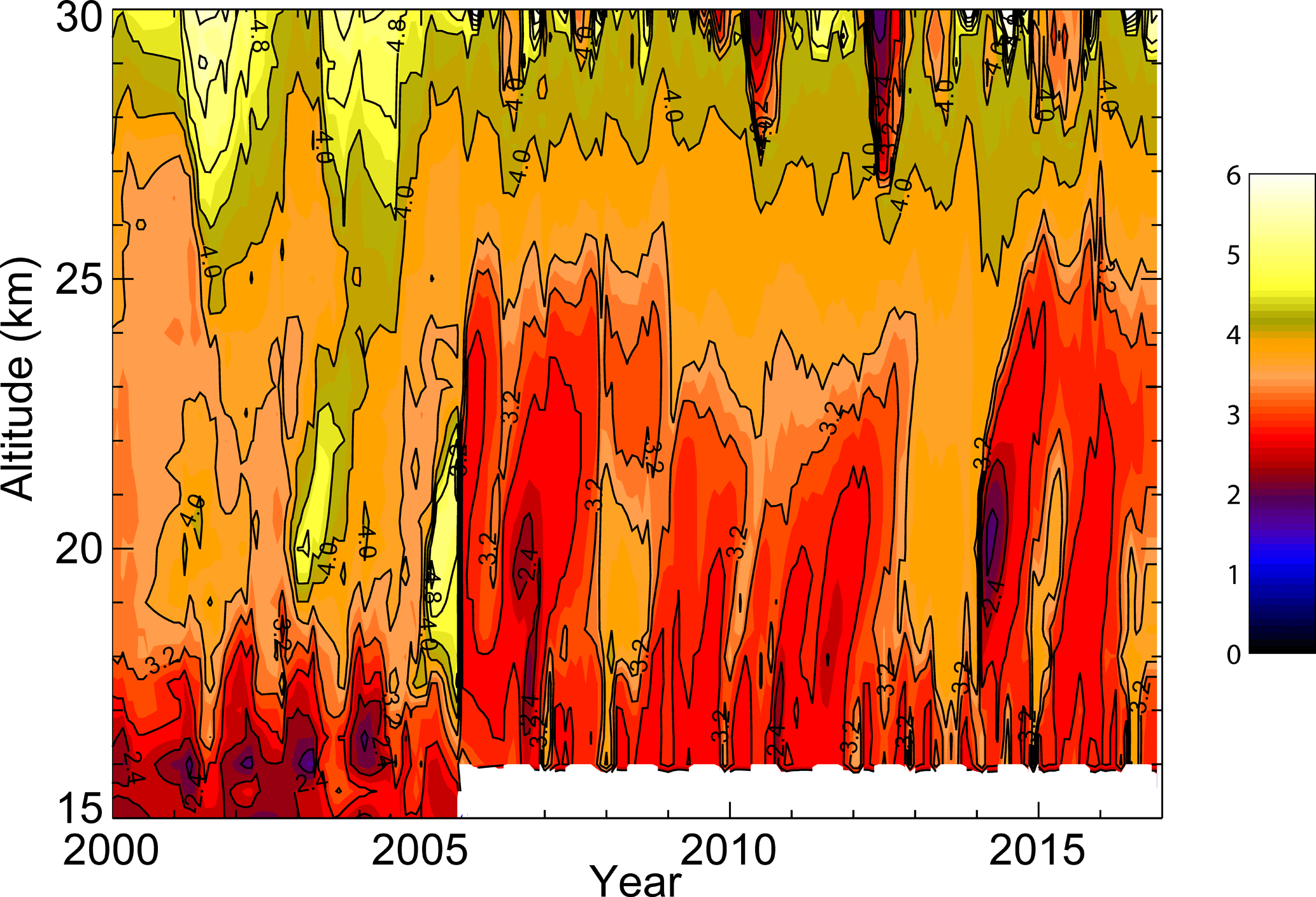
Figure 15Ratio of GloSSAC 525 to 1020 nm extinction coefficient at 2.5∘ N for 2000 to 2016. The switch from primarily SAGE II to OSIRIS occurs in mid-2005 with CALIPSO also contributing, beginning in mid-2006.
The second issue we observe in the OSIRIS/CALIPSO period is that aerosol extinction is higher in the lower stratosphere (below 20 km) in mid- and high latitudes of both hemispheres than typically observed in the similar SAGE II period leading up to that segment. It appears to be associated with data from both OSIRIS and CALIPSO and may simply be the outcome of regular volcanic events throughout this period. The primary sink for aerosol is through polar latitudes and enhancements in extinction are even expected following low latitude eruptions. However, the elevated levels appear to persist into less active periods and are manifested fairly equally in both hemispheres, while volcanic activity occurred mostly in the Northern Hemisphere. It is possible that the GloSSAC depiction is correct; however, an unexpected disconnect between SAGE II and OSIRIS/CALIPSO data is of concern and users should be aware of some issues in this time and region. For CALIPSO backscatter data, it is possible that improving the backscatter coefficient to extinction coefficient conversion may reduce the apparent discrepancy. In addition, with the beginning of SAGE III's mission aboard the ISS in 2017, we hope to use those new data to understand this issue. We also plan to examine SCIAMACHY and/or OMPS as contributors to this issue as well as to GloSSAC in general.
5.1 GloSSAC quality assessment
As a data product intended for use by the climate modeling community, it is critical to deal with as many issues in the data set as possible and not leave those issues for the users to discover on their own. While the data used in GloSSAC are generally robust, it is still common for occasional bad individual values or entire profiles to occur and have a deleterious impact on the data set if accepted as truth. As a result, we have implemented a quality assurance process to identify and remove low quality data from GloSSAC. Although we considered a number of automated schemes to identify “bad” data, the most effective means was a month-by-month visual examination of the data. In this case, we identify bad data points/profiles using our best scientific judgment and remove them from the data set. We only remove data when the impact is obvious and we apply it only to the final 1020 and 525 nm data products. While issues typically appear in both wavelengths, they occasionally occur at only one wavelength and we deal with these individually. The extinction products consist of a little more than 1 million individual values, and in quality assurance we identify less than 5000 bad data point or less than 0.5 % of all data values (roughly the equivalent of 2 months in 38 years). In the SAGE II period, these data points tend to occur at high latitude where we have noted (albeit rarely) data quality issues in the past. Once the bad data points are removed, we interpolate the data across any new gaps using the same approach used in other processes. Data replaced in this manner are flagged.
5.2 High altitude climatology for the OSIRIS/CALIPSO period
We have created a SAGE-II-based monthly climatology for altitudes above 30 km to replace OSIRIS and CALIPSO data. In general, neither of these data sets is consistent with SAGE II above that altitude (where extinction is very low), whereas SAGE II is generally robust to higher altitudes. In this climatology, we average all SAGE II data for each month except the years 1991 to 1994, where Pinatubo effects were obvious above 30 km. Any OSIRIS or CALIPSO data above 30 km at 525 and 1020 nm is replaced with the climatology and flagged.
5.3 Stratospheric background
A nominal stratospheric background is included as a part of the GloSSAC data set. It consists of the average of 1999, 2000, 2001, 2003, and 2004; we excluded 2002 because of the eruption of Ruang in September of that year. The year 2000 is the lowest aerosol extinction in the entire record and it could be used as a background level. However, there is a notable effect of the quasi-biennial oscillation (QBO) on aerosol extinction above 20 km (Thomason et al., 1997a) and using 2000 as the background year in a repeating series has discontinuities as large as a factor of 2 every January. The 5-year average, while generally slightly larger than 2000 levels, effectively removes most if not all QBO-related discontinuities.
5.4 Derived aerosol products
The focus of the GloSSAC data set is aerosol optical measurements; however, there is substantial interest in aerosol properties that are derivable from these properties, particularly aerosol surface area density and effective radius. As a result, we have included values for these parameters where SAGE II measurements are available. They are derived using the method described in Thomason et al. (2008) and consistent with the same properties included in the native SAGE II version 7 data set and designed to bracket the potential range in these parameters. These data are included for informational purposes and they should not be interpreted as canonical estimates for them.
5.5 GloSSAC parameter uncertainty
Measurement uncertainties are included in the data set only for the SAGE II portion of the data sets. In this regard for each latitude/time/altitude bin, we include the standard deviation of the measurements used (a combination of geophysical variability and measurement noise) and the median reported measurement uncertainty. Generally, SAGE II aerosol extinction coefficients in the lower stratosphere have uncertainties of less than 10 % and, during Pinatubo, often less than 5 %. The same uncertainty parameters for all space-based measurements, including new potential data sources SCIAMACHY and SAGE III/ISS, will be included in the next GloSSAC release. Beyond measurement uncertainty, the conversion of one measured quantity to another adds the potential for significant and variable bias to GloSSAC values at 525 and 1020 nm. The process we used to scale data from OSIRIS, CLAES, HALOE, and CALIPSO to the long-term 525 and 1020 nm data sets nominally eliminate bias from between the data sets and the spread of measurements is more or less the combined measurements uncertainty combined with geophysical variability. However, this is only the case where the data sets overlap. For CLAES/HALOE, their use in GloSSAC coincides with the massively volcanic Pinatubo period and their sole use is for altitudes/latitudes where SAGE II data does not exist. For CALIPSO/OSIRIS, their use is solely for the period after the SAGE II mission ends. A complicating factor for this period is that the overlap period between SAGE II and OSIRIS was volcanically quiescent while much of the period after 2005 consists of a steady drumbeat of small but significant volcanic events. There are few independent robust measurements for either the Pinatubo period (particularly in the tropics) or the post-SAGE II period. As a result, it is difficult to evaluate how well the conversion processes work and there is the potential for bias. We hope the new SAGE III mission in this mildly volcanic period will give insights into the potential for bias with both OSIRIS and CALIPSO as well as suggest mechanisms for migrating any issues. This is a focus for future developments in GloSSAC.
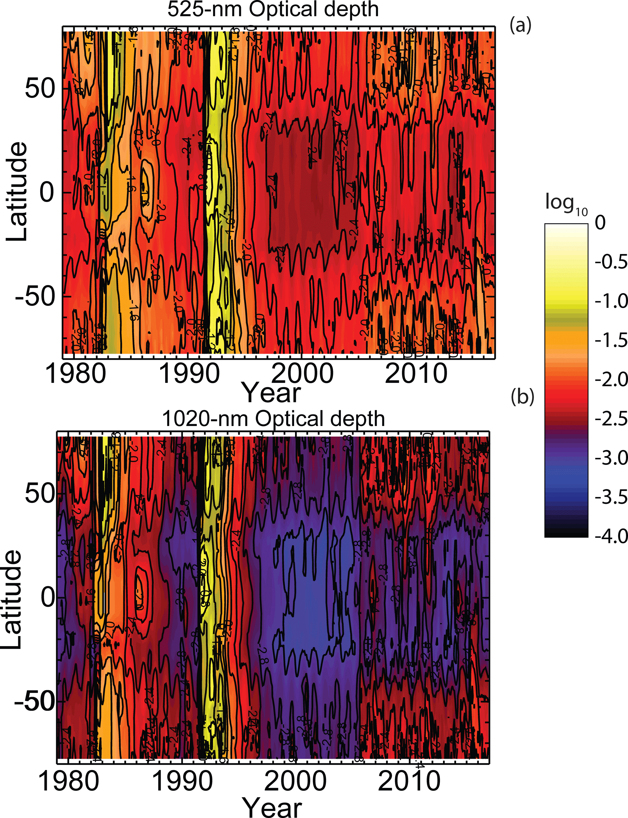
Figure 16Total GloSSAC stratospheric aerosol optical depth at 525 (a) and 1020 nm (b). We show contours at 0.0006, 0.0008, 0.001, 0.002, 0.004, 0.006, 0.008, 0.01, 0.02, 0.04, 0.06, 0.08, 0.1, 0.15, 0.2, and 0.4.
5.6 Stratospheric optical depth
Stratospheric optical depth at 525 and 1020 nm integrated from a base at the tropopause upwards can be easily computed using components of the GloSSAC data set. These are shown in Fig. 16. The GloSSAC minimum 525 nm optical depth in the tropics (0.0028) occurs in May 2001 as an extended period of very limited volcanic influence was terminated by the eruption of Ruang (Indonesia) in October 2002 and subsequent eruptions. The peak optical depth at 525 nm is 0.22 and occurs in the tropics several months after Pinatubo in November 1991. Although the delay is not an obvious outcome, several factors contribute to this feature. Given that the primary injection altitude was well above 20 km, there would be little loss of aerosol from the stratosphere in the first months following the eruption. Also, since a significant fraction of what would become sulfate aerosol entered the stratosphere as SO2 gas, the conversion for SO2 to H2SO4 (with nominally about a 30-day time constant) would tend to delay the peak in the mass of aerosol for a few months (Shen et al., 2015). It is also likely that there was significant formation of new and very small particles that would require some time for coagulation to increase their size sufficiently to affect visible wavelength extinction (≥ 0.1 µm).
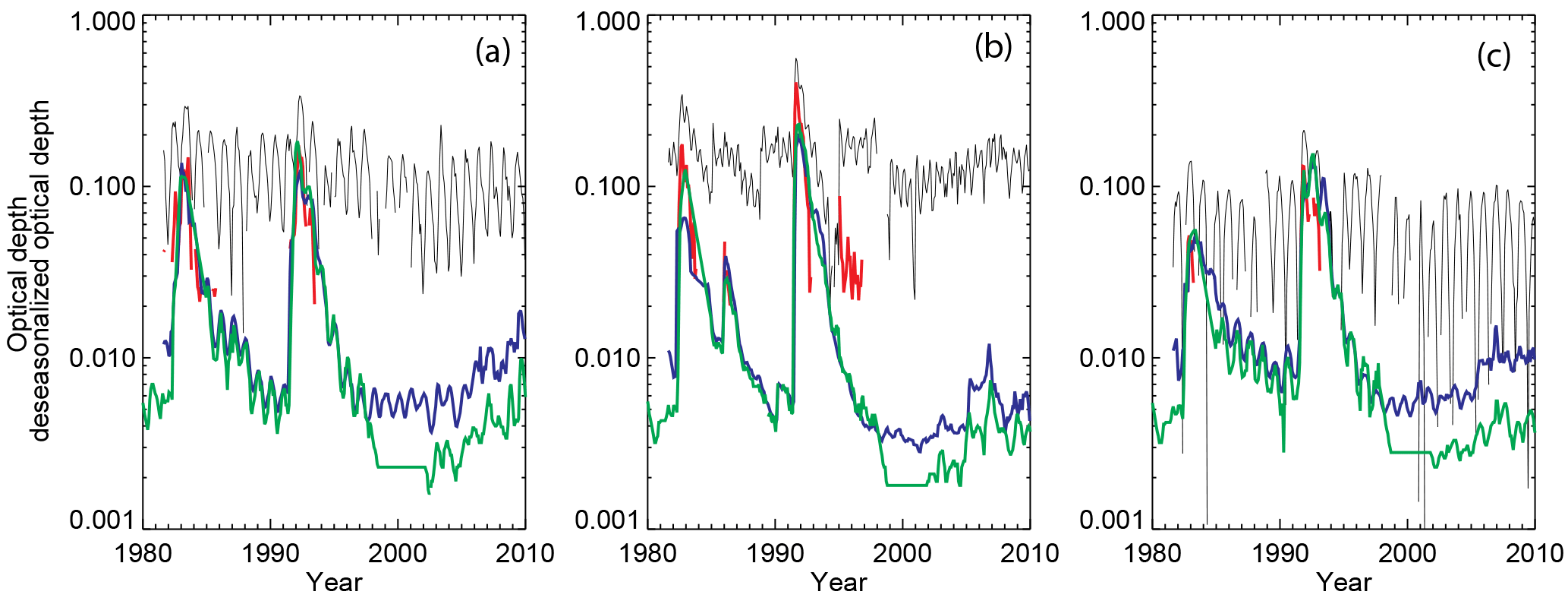
Figure 17Comparison of total stratospheric aerosol optical depth at northern midlatitudes, the tropics, and southern midlatitudes at 525 (SAGE II/GISS) and 550 nm (AVHRR). AVHRR is shown in black, AVHRR with a 28-year median annual cycle removed is red, GloSSAC is shown in blue, and the GISS data set is shown in green.
Figure 17 shows a comparison of GloSSAC 525 nm optical depth, Version 2.0 of the Advanced Very High Resolution Radiometer (AVHRR) total atmospheric aerosol optical depth (Zhao, 2013; Zhao and Chan, 2014), and the GISS stratospheric aerosol 500 nm optical depth (Sato et al., 1993). AVHRR provides a measurement of total atmospheric aerosol optical depth at 500 nm. Aerosol optical depth is usually dominated by tropospheric aerosol and variability in the stratosphere is not apparent. This is not the case following large volcanic events where the volcanic perturbation can be larger than the tropospheric component. For comparison purposes, we remove the 28-year median annual cycle from the long-term AVHRR record to highlight the impact of the Pinatubo and El Chichón eruptions. In addition, we plot AVHRR data only during the first years after both eruptions as AVHRR is unable to infer stratospheric effects once the stratospheric optical depth is much less than about 0.02. Figure 17 shows the AVHRR total and “stratospheric” optical depth. While there is reasonable agreement between the AVHRR and GloSSAC data products in midlatitudes, the tropical optical depths show a substantial difference for both eruptions. For Pinatubo, it suggests a tropical total optical depth in excess of 0.4 (at 500 nm), which is substantially larger than the corresponding value of 0.22 in the GloSSAC stratospheric optical depth. Some of the difference could be due to loading in the upper troposphere that is not a part of the GloSSAC stratospheric optical depth (integrated from the tropopause upward) but that AVHRR includes. It is also likely that setting a baseline is partly responsible for this issue. On the one hand, if only the few years prior to the Pinatubo eruption are used, the peak optical depth from AVHRR decreases to about 0.3. On the other hand, the optical depth after early 1993 is less than and becomes much less than the background values from the pre-Pinatubo period. At least in the tropics, it is also clear there are some discontinuities in the optical record that appear to be unrelated to geophysical phenomena. In any case, the AVHRR peak Pinatubo optical depth is between 50 and 100 % larger than that from GloSSAC.
In order for the AVHRR/GloSSAC difference to be due purely to stratospheric aerosol, the mostly likely GloSSAC-related culprit would be the conversion of CLAES infrared observations to SAGE II wavelengths. The correction from CLAES to SAGE would have to be in error by a factor of about 2. The correlation between SAGE II and CLAES observations (Fig. 6) is well behaved and provide little suggestion that an error on that scale is possible. Sun photometer measurements from sites in American Samoa, Mauna Loa, and other sites (Dutton et al., 1994; Stone et al., 1993; Russell et al., 1996; Dutton and Christy, 1992) suggest a peak mid-visible optical depth between 0.2 and 0.25 and perhaps as large as 0.3. The GloSSAC value is on the low end of these values but the Sun photometer measurements will also include volcanic aerosol in the troposphere. As a result, we believe that GloSSAC stratospheric optical depths for the Pinatubo period are reasonable. The GISS data set after 1979 is based on the data from the same instruments used in GloSSAC and a good level of agreement would be expected. In general, that is observed until at least 1998 (Fig. 17). There are some minor differences most likely related to updates in SAGE data products, changes in cloud clearing, and the filling process. After 1998, however, the GISS optical depth is uniformly about a factor of 2 less than GloSSAC values with an almost immediate transition from reasonable to poor agreement. The large differences between these data sets after 1998, particularly up to the end of the SAGE II period in 2005, are difficult to understand and the GISS values appear to be in error. Overall, we do not recommend the use of AVHRR or GISS for validating CCM estimates for stratospheric column optical depth. On the other hand, users of GloSSAC should be aware that there is almost certainly substantial aerosol in the upper troposphere particularly in the tropics during the several months if not a few years following the Pinatubo eruption. That material is not a part of the stratospheric GloSSAC data set yet may have significant climate influence.
GloSSAC version 1.0 is available in netCDF format at the NASA Atmospheric Data Center at https://eosweb.larc.nasa.gov/. GloSSAC users should cite this paper and the data set DOI (https://doi.org/10.5067/GloSSAC-L3-V1.0).
Despite some limitations, we believe that this is by far the best data set in this series of data sets (ASAP, CCMI). Compared to previous releases of the data set such as ASAP or the set for CCMI in 2014, we have implement a number of major improvements. These include the handling of the Pinatubo SAGE II saturation period in 1991 to 1993, the way in which missing values at high latitudes are filled during the entire SAGE II period, and how the post-SAGE II period is constructed using OSIRIS and CALIPSO. The data set is focused on providing as close to measured aerosol optical properties as possible. Recognizing the complexity of mixing data from many sources, unmodified source data are preserved in the data set at the GloSSAC resolution.
For users, we recommend the following practices for this data set:
-
For validation of aerosol properties derived within a chemistry-climate model, we suggest that the most robust comparisons are with the measurements directly. As a result, we suggest that they use the data flags to identify these values in the data set and compare model-derived parameters with those identified as measured, as opposed to indirectly inferred values.
-
We have not focused on the derivation of bulk aerosol properties within this data set though it is suitable for that process. Even though values are reported at 525 and 1020 nm for every grid box, it is critical to recognize when data are based on a single measurement wavelength. This includes everything outside the SAGE II period and some data gap periods within the SAGE II period associated with Pinatubo. Users who wish to use this data set for developing climatologies of aerosol properties are welcome to do so as well as distribute any products derived from your effort. We would appreciate attribution of the source material.
The summary of key issues associated with the data set are the following:
-
The summer of 1991 in the tropics is poorly resolved due to the loss of SAGE II in the lower stratosphere and because CLAES data do not become available until October of that year. In any case, the highly inhomogeneous state of the stratosphere in the several months following the Pinatubo eruption makes a monthly depiction of questionable validity.
-
The OSIRIS/CALIPSO period presents two issues. There is clearly an issue with converting measurements from 525 to 1020 nm and the later data should be used very cautiously. This is a one-wavelength period where only 525 nm values should be used. Also, there are high levels of aerosol extinction in the lower stratosphere throughout this segment of the data set. While we cannot exclude that it is correct, users should exercise caution with these data.
-
Data in the troposphere is only reported during the SAGE II period and only away from the Pinatubo eruption. It is likely that there is considerable aerosol in the upper troposphere during this period but we have little ability to produce values based on measurements in this period. While tropospheric aerosol is not the general area of concern for GloSSAC, it is likely that volcanic aerosol in the upper tropical troposphere plays a role in changing climate during the aftermath of the Pinatubo eruption.
We plan to release new versions in about a yearly cycle. Extensions of the data set using the current processing paradigm will be indicated by minor version number changes (ie., 1.0 to 1.1). If new data sources or significant processing changes occur, the version will change the major number (i.e., 1.0 to 2.0). Current plans are to release version 2.0 in 2018 with the addition of at least SAGE III/ISS data at the end of the record. We will also look at other newer data sets particularly the available SCIAMACHY data set but also aerosol products from OMPS and AerGOM. We may look into deriving data at a higher temporal resolution to more fully utilize the data afforded by OSIRIS and CALIPSO. For the SAGE period, we may examine the approach for deriving ozone variability described in Damadeo et al. (2014). Feedback from users will also be useful in updates to the data set.
In the past, this data product was mostly an “in-house” intermediate product not readily available to the science community. This new approach, and this paper, is an effort to make it more transparent and accessible to all potential users.
| ACE | Atmospheric Chemistry Experiment |
| AerGOM | an improved algorithm for stratospheric aerosol extinction retrieval from GOMOS |
| ASAP | Assessment of Stratospheric Aerosol Properties |
| AVHRR | Advanced Very High Resolution Radiometer |
| CALIPSO | Cloud-Aerosol Lidar and Infrared Pathfinder Satellite Observation |
| CCM | chemistry-climate model |
| CCMI | Chemistry-Climate Model Intercomparison SPARC actvity |
| CLAES | Cryogenic Limb Array Etalon Spectrometer |
| CMIP | Climate Model Intercomparison Project |
| ESRL | Earth System Research Laboratory |
| GEOS | Goddard Earth Observing System Model |
| GISS | Goddard Institute for Space Studies |
| GloSSAC | Global Space-based Stratospheric Aerosol Climatology |
| GOMOS | Global Ozone Monitoring by Occultation of Stars |
| HALOE | Halogen Occultation Experiment |
| HIRDLS | High Resolution Dynamics Limb Sounder |
| ILAS I/II | Improved Limb Atmospheric Sounder |
| ISS | International Space Station |
| MAESTRO | Measurements of Aerosol Extinction in the Stratosphere and Troposphere Retrieved by Occultation |
| MERRA | Modern-Era Retrospective analysis for Research and Applications, Version 2 |
| NASA | National Aeronautics and Space Administration |
| NAT | nitric acid trihydrate |
| NOAA | National Oceanographic and Atmospheric Administration |
| OMPS | Ozone Mapping Profiler Suite |
| OSIRIS | Optical Spectrograph and InfraRed Imager System |
| POAM III | Polar Ozone and Aerosol Measurement |
| PSC | polar stratospheric cloud |
| SCIAMACHY | SCanning Imaging Absorption spectrometer for Atmospheric CartograpHY |
| SAM | Stratospheric Aerosol Measurement |
| SAGE | Stratospheric Aerosol and Gas Experiment |
| SOFIE | Solar Occultation for Ice Experiment |
| SPARC | Stratospheric-tropospheric Processes and their Role in Climate |
| STS | saturated ternary solution |
| UARS | Upper Atmosphere Research Satellite |
| WMO | World Meteorological Organization |
The authors declare that they have no conflict of interest.
This article is part of the special issue “Chemistry–Climate Modeling Initiative (CCMI) (ACP/AMT/ESSD/GMD inter-journal SI)”. It is not associated with a conference.
The authors would like to thank Andrea Gettleman, editor, and Matthew Toohey
and Chaochao Gao, reviewers, for suggestions and comments that improved the
content of this paper.
Edited by: Andrew Gettelman
Reviewed by: Matthew Toohey and Chaochao Gao
Antuña, J. C.: Lidar measurements of stratospheric aerosols from Mount Pinatubo at Camagüey, Cuba, Atmos. Environ., 30, 1857–1860, https://doi.org/10.1016/1352-2310(95)00386-X, 1996.
Arfeuille, F., Luo, B. P., Heckendorn, P., Weisenstein, D., Sheng, J. X., Rozanov, E., Schraner, M., Brönnimann, S., Thomason, L. W., and Peter, T.: Modeling the stratospheric warming following the Mt. Pinatubo eruption: uncertainties in aerosol extinctions, Atmos. Chem. Phys., 13, 11221–11234, https://doi.org/10.5194/acp-13-11221-2013, 2013.
Barnes, J. E. and Hofmann, D. J.: Lidar measurements of stratospheric aerosol over Mauna Loa Observatory, Geophys. Res. Lett., 24, 1923–1926, https://doi.org/10.1029/97gl01943, 1997.
Bauman, J. J., Russell, P. B., Geller, M. A., and Hamill, P.: A stratospheric aerosol climatology from SAGE II and CLAES measurements: 1. Methodology, J. Geophys. Res.-Atmos., 108, 4382, https://doi.org/10.1029/2002jd002992, 2003.
Bevilacqua, R. M., Aellig, C. P., Debrestian, D. J., Fromm, M. D., Hoppel, K., Lumpe, J. D., Shettle, E. P., Hornstein, J. S., Randall, C. E., Rusch, D. W., and Rosenfield, J. E.: POAM II ozone observations in the Antarctic ozone hole in 1994, 1995, and 1996, J. Geophys. Res.-Atmos., 102, 23643–23657, https://doi.org/10.1029/97jd01623, 1997.
Burton, S. P., Thomason, L. W., Sasano, Y., and Hayashida, S.: Comparison of aerosol extinction measurement by ILAS and SAGE II, Geophys. Res. Lett., 26, 1719–1722, https://doi.org/10.1029/1999gl900359, 1999.
Damadeo, R. P., Zawodny, J. M., Thomason, L. W., and Iyer, N.: SAGE version 7.0 algorithm: application to SAGE II, Atmos. Meas. Tech., 6, 3539–3561, https://doi.org/10.5194/amt-6-3539-2013, 2013.
Damadeo, R. P., Zawodny, J. M., and Thomason, L. W.: Reevaluation of stratospheric ozone trends from SAGE II data using a simultaneous temporal and spatial analysis, Atmos. Chem. Phys., 14, 13455–13470, https://doi.org/10.5194/acp-14-13455-2014, 2014.
Dutton, E. G. and Christy, J. R.: Solar Radiative Forcing at Selected Locations and Evidence for Global Lower Tropospheric Cooling Following the Eruptions of El-Chichon and Pinatubo, Geophys. Res. Lett., 19, 2313–2316, https://doi.org/10.1029/92gl02495, 1992.
Dutton, E. G., Reddy, P., Ryan, S., and Deluisi, J. J.: Features and Effects of Aerosol Optical Depth Observed at Mauna-Loa, Hawaii – 1982–1992, J. Geophys. Res.-Atmos., 99, 8295–8306, https://doi.org/10.1029/93jd03520, 1994.
GloSSAC Team: Global Space-based Stratospheric Aerosol Climatology, Hampton, VA, USA: NASA Atmospheric Science Data Center (ASDC), https://doi.org/10.5067/GloSSAC-L3-V1.0, 2017.
Gorkavyi, N., Rault, D. F., Newman, P. A., da Silva, A. M., and Dudorov, A. E.: New stratospheric dust belt due to the Chelyabinsk bolide, Geophys. Res. Lett., 40, 4728–4733, https://doi.org/10.1002/grl.50788, 2013.
Eparvier, F. G., Rusch, D. W., Clancy, R. T., and Thomas, G. E.: Solar Mesosphere Explorer satellite measurements of El Chichón stratospheric aerosols: 2. Aerosol mass and size parameters, J. Geophys. Res., 99, 20533–20544, https://doi.org/10.1029/94JD01841, 1994.
Hervig, M. E., Bardeen, C. G., Siskind, D. E., Mills, M. J., and Stockwell, R.: Meteoric smoke and H2SO4 aerosols in the upper stratosphere and mesosphere, Geophys. Res. Lett., 44, 1150–1157, https://doi.org/10.1002/2016GL072049, 2017.
Jager, H. and Hofmann, D.: Midlatitude lidar backscatter to mass, area, and extinction conversion model based on in situ aerosol measurements from 1980 to 1987, Appl. Opt., 30, 127–138, https://doi.org/10.1364/AO.30.000127, 1991.
Jäger, H., Deshler, T., and Hofmann, D. J.: Midlatitude lidar backscatter conversions based on balloonborne aerosol measurements, Geophys. Res. Lett., 22, 1729–1732, https://doi.org/10.1029/95GL01521, 1995.
Kar, J., McElroy, C. T., Drummond, J. R., Zou, J., Nichitiu, F., Walker, K. A., Randall, C. E., Nowlan, C. R., Dufour, D. G., Boone, C. D., Bernath, P. F., Trepte, C. R., Thomason, L. W., and McLinden, C.: Initial comparison of ozone and NO2 profiles from ACE-MAESTRO with balloon and satellite data, J. Geophys. Res.-Atmos., 112, D16301, https://doi.org/10.1029/2006jd008242, 2007.
Kent, G. S., Trepte, C. R., Farrukh, U. O., and Mccormick, M. P.: Variation in the Stratospheric Aerosol Associated with the North Cyclonic Polar Vortex as Measured by the Sam-Ii Satellite Sensor, J. Atmos. Sci., 42, 1536–1551, https://doi.org/10.1175/1520-0469(1985)042<1536:Vitsaa>2.0.Co;2, 1985.
Kent, G. S., Trepte, C. R., Wang, P. H., and Lucker, P. L.: Problems in separating aerosol and cloud in the Stratospheric Aerosol and Gas Experiment (SAGE) II data set under conditions of lofted dust: Application to the Asian deserts, J. Geophys. Res.-Atmos., 108, 4410, https://doi.org/10.1029/2002jd002412, 2003.
Lambert, A., Grainger, R. G., Remedios, J. J., Reburn, W. J., Rodgers, C. D., Taylor, F. W., Roche, A. E., Kumer, J. B., Massie, S. T., and Deshler, T.: Validation of aerosol measurements from the improved stratospheric and mesospheric sounder, J. Geophys. Res.-Atmos., 101, 9811–9830, https://doi.org/10.1029/95jd01702, 1996.
Manney, G. L., Michelsen, H. A., Santee, M. L., Gunson, M. R., Irion, F. W., Roche, A. E., and Livesey, N. J.: Polar vortex dynamics during spring and fall diagnosed using trace gas observations from the Atmospheric Trace Molecule Spectroscopy instrument, J. Geophys. Res.-Atmos., 104, 18841–18866, https://doi.org/10.1029/1999JD900317, 1999.
Manney, G. L., Michelsen, H. A., Bevilacqua, R. M., Gunson, M. R., Irion, F. W., Livesey, N. J., Oberheide, J., Riese, M., Russell, J. M., Toon, G. C., and Zawodny, J. M.: Comparison of satellite ozone observations in coincident air masses in early November 1994, J. Geophys. Res.-Atmos., 106, 9923–9943, https://doi.org/10.1029/2000JD900826, 2001.
Manney, G. L., Daffer, W. H., Zawodny, J. M., Bernath, P. F., Hoppel, K. W., Walker, K. A., Knosp, B. W., Boone, C., Remsberg, E. E., Santee, M. L., Harvey, V. L., Pawson, S., Jackson, D. R., Deaver, L., McElroy, C. T., McLinden, C. A., Drummond, J. R., Pumphrey, H. C., Lambert, A., Schwartz, M. J., Froidevaux, L., McLeod, S., Takacs, L. L., Suarez, M. J., Trepte, C. R., Cuddy, D. C., Livesey, N. J., Harwood, R. S., and Waters, J. W.: Solar occultation satellite data and derived meteorological products: Sampling issues and comparisons with Aura Microwave Limb Sounder, J. Geophys. Res.-Atmos., 112, D24S50, https://doi.org/10.1029/2007JD008709, 2007.
Massie, S. T., Gille, J. C., Edwards, D. P., Bailey, P. L., Lyjak, L. V., Craig, C. A., Cavanaugh, C. P., Mergenthaler, J. L., Roche, A. E., Kumer, J. B., Lambert, A., Grainger, R. G., Rodgers, C. D., Taylor, F. W., Russell, J. M., Park, J. H., Deshler, T., Hervig, M. E., Fishbein, E. F., Waters, J. W., and Lahoz, W. A.: Validation studies using multiwavelength cryogenic limb array etalon spectrometer (CLAES) observations of stratospheric aerosol, J. Geophys. Res.-Atmos., 101, 9757–9773, https://doi.org/10.1029/95jd03225, 1996.
Massie, S. T., Gille, J., Craig, C., Khosravi, R., Barnett, J., Read, W., and Winker, D.: HIRDLS and CALIPSO observations of tropical cirrus, J. Geophys. Res.-Atmos., 115, D00H11, https://doi.org/10.1029/2009JD012100, 2010.
Mills, M. J., Schmidt, A., Easter, R., Solomon, S., Kinnison, D. E., Ghan, S. J., Neely, R. R., Marsh, D. R., Conley, A., Bardeen, C. G., and Gettelman, A.: Global volcanic aerosol properties derived from emissions, 1990–2014, using CESM1(WACCM), J. Geophys. Res.-Atmos., 121, 2332–2348, https://doi.org/10.1002/2015jd024290, 2016.
Morgenstern, O., Hegglin, M. I., Rozanov, E., O'Connor, F. M., Abraham, N. L., Akiyoshi, H., Archibald, A. T., Bekki, S., Butchart, N., Chipperfield, M. P., Deushi, M., Dhomse, S. S., Garcia, R. R., Hardiman, S. C., Horowitz, L. W., Jöckel, P., Josse, B., Kinnison, D., Lin, M., Mancini, E., Manyin, M. E., Marchand, M., Marécal, V., Michou, M., Oman, L. D., Pitari, G., Plummer, D. A., Revell, L. E., Saint-Martin, D., Schofield, R., Stenke, A., Stone, K., Sudo, K., Tanaka, T. Y., Tilmes, S., Yamashita, Y., Yoshida, K., and Zeng, G.: Review of the global models used within phase 1 of the Chemistry–Climate Model Initiative (CCMI), Geosci. Model Dev., 10, 639–671, https://doi.org/10.5194/gmd-10-639-2017, 2017.
Osborn, M. T., Decoursey, R. J., Trepte, C. R., Winker, D. M., and Woods, D. C.: Evolution of the Pinatubo Volcanic Cloud over Hampton, Virginia, Geophys. Res. Lett., 22, 1101–1104, https://doi.org/10.1029/95gl00815, 1995.
Poole, L. R. and Pitts, M. C.: Polar stratospheric cloud climatology based on Stratospheric Aerosol Measurement II observations from 1978 to 1989, J. Geophys. Res.-Atmos., 99, 13083–13089, https://doi.org/10.1029/94JD00411, 1994.
Randall, C. E., Bevilacqua, R. M., Lumpe, J. D., and Hoppel, K. W.: Validation of POAM III aerosols: Comparison to SAGE II and HALOE, J. Geophys. Res.-Atmos., 106, 27525–27536, https://doi.org/10.1029/2001jd000528, 2001.
Randall, C. E., Manney, G. L., Allen, D. R., Bevilacqua, R. M., Hornstein, J., Trepte, C., Lahoz, W., Ajtic, J., and Bodeker, G.: Reconstruction and Simulation of Stratospheric Ozone Distributions during the 2002 Austral Winter, J. Atmos. Sci., 62, 748–764, https://doi.org/10.1175/jas-3336.1, 2005.
Rieger, L. A., Bourassa, A. E., and Degenstein, D. A.: A merged SAGE II-OSIRIS stratospheric aerosol record, J. Geophys. Res., 120, 8890–8904, https://doi.org/10.1002/2015jd023133, 2015.
Rienecker, M. M., Suarez, M. J., Gelaro, R., Todling, R., Bacmeister, J., Liu, E., Bosilovich, M. G., Schubert, S. D., Takacs, L., Kim, G. K., Bloom, S., Chen, J. Y., Collins, D., Conaty, A., Da Silva, A., Gu, W., Joiner, J., Koster, R. D., Lucchesi, R., Molod, A., Owens, T., Pawson, S., Pegion, P., Redder, C. R., Reichle, R., Robertson, F. R., Ruddick, A. G., Sienkiewicz, M., and Woollen, J.: MERRA: NASA's Modern-Era Retrospective Analysis for Research and Applications, J. Climate, 24, 3624–3648, https://doi.org/10.1175/Jcli-D-11-00015.1, 2011.
Robert, C. É., Bingen, C., Vanhellemont, F., Mateshvili, N., Dekemper, E., Tétard, C., Fussen, D., Bourassa, A., and Zehner, C.: AerGOM, an improved algorithm for stratospheric aerosol extinction retrieval from GOMOS observations – Part 2: Intercomparisons, Atmos. Meas. Tech., 9, 4701–4718, https://doi.org/10.5194/amt-9-4701-2016, 2016.
Rogers, R. R., Hostetler, C. A., Hair, J. W., Ferrare, R. A., Liu, Z., Obland, M. D., Harper, D. B., Cook, A. L., Powell, K. A., Vaughan, M. A., and Winker, D. M.: Assessment of the CALIPSO Lidar 532 nm attenuated backscatter calibration using the NASA LaRC airborne High Spectral Resolution Lidar, Atmos. Chem. Phys., 11, 1295–1311, https://doi.org/10.5194/acp-11-1295-2011, 2011.
Rosen, J. M. and Kjome, N. T.: Backscattersonde: a new instrument for atmospheric aerosol research, Appl. Opt., 30, 1552–1561, 10.1364/AO.30.001552, 1991.
Rosen, J. M., Kjome, N. T., and Liley, J. B.: Tropospheric aerosol backscatter at a midlatitude site in the northern and southern hemispheres, J. Geophys. Res.-Atmos., 102, 21329–21339, https://doi.org/10.1029/97jd01486, 1997.
Russell, P. B., Livingston, J. M., Pueschel, R. F., Bauman, J. J., Pollack, J. B., Brooks, S. L., Hamill, P., Thomason, L. W., Stowe, L. L., Deshler, T., Dutton, E. G., and Bergstrom, R. W.: Global to microscale evolution of the Pinatubo volcanic aerosol derived from diverse measurements and analyses, J. Geophys. Res.-Atmos., 101, 18745–18763, https://doi.org/10.1029/96jd01162, 1996.
Sato, M., Hansen, J. E., Mccormick, M. P., and Pollack, J. B.: Stratospheric Aerosol Optical Depths, 1850–1990, J. Geophys. Res.-Atmos., 98, 22987–22994, https://doi.org/10.1029/93jd02553, 1993.
Schoeberl, M. R., Lait, L. R., Newman, P. A., Martin, R. L., Proffitt, M. H., Hartmann, D. L., Loewenstein, M., Podolske, J., Strahan, S. E., Anderson, J., Chan, K. R., and Gary, B.: Reconstruction of the Constituent Distribution and Trends in the Antarctic Polar Vortex from Er-2 Flight Observations, J. Geophys. Res.-Atmos., 94, 16815–16845, https://doi.org/10.1029/JD094iD14p16815, 1989.
Sheng, J.-X., Weisenstein, D. K., Luo, B.-P., Rozanov, E., Arfeuille, F., and Peter, T.: A perturbed parameter model ensemble to investigate Mt. Pinatubo's 1991 initial sulfur mass emission, Atmos. Chem. Phys., 15, 11501–11512, https://doi.org/10.5194/acp-15-11501-2015, 2015.
Solomon, S., Daniel, J. S., Neely III, R. R., Vernier, J. P., Dutton, E. G., and Thomason, L. W.: The persistently variable “background” stratospheric aerosol layer and global climate change, Science, 333, 866–870, https://doi.org/10.1126/science.1206027, 2011.
SPARC: Assessment of Stratospheric Aerosol Properties (ASAP), SPARC Report, WCRP-124, WMO/TD No. 1295, SPARC Report No. 4, 348 pp., 2006.
Stenchikov, G. L., Kirchner, I., Robock, A., Graf, H. F., Antuña, J. C., Grainger, R. G., Lambert, A., and Thomason, L.: Radiative forcing from the 1991 Mount Pinatubo volcanic eruption, J. Geophys. Res.-Atmos., 103, 13837–13857, https://doi.org/10.1029/98jd00693, 1998.
Stone, R. S., Key, J. R., and Dutton, E. G.: Properties and Decay of Stratospheric Aerosols in the Arctic Following the 1991 Eruptions of Mount-Pinatubo, Geophys. Res. Lett., 20, 2359–2362, https://doi.org/10.1029/93gl02684, 1993.
Taylor, K. E., Stouffer, R. J., and Meehl, G. A.: An Overview of Cmip5 and the Experiment Design, B. Am. Meteorol. Soc., 93, 485–498, https://doi.org/10.1175/BAMS-D-11-00094.1, 2012.
Thomason, L. W.: Toward a combined SAGE II-HALOE aerosol climatology: an evaluation of HALOE version 19 stratospheric aerosol extinction coefficient observations, Atmos. Chem. Phys., 12, 8177–8188, https://doi.org/10.5194/acp-12-8177-2012, 2012.
Thomason, L. W. and Osborn, M. T.: Lidar Conversion Parameters Derived from Sage-Ii Extinction Measurements, Geophys. Res. Lett., 19, 1655–1658, https://doi.org/10.1029/92gl01619, 1992.
Thomason, L. W. and Vernier, J.-P.: Improved SAGE II cloud/aerosol categorization and observations of the Asian tropopause aerosol layer: 1989–2005, Atmos. Chem. Phys., 13, 4605–4616, https://doi.org/10.5194/acp-13-4605-2013, 2013.
Thomason, L. W., Kent, G. S., Trepte, C. R., and Poole, L. R.: A comparison of the stratospheric aerosol background periods of 1979 and 1989–1991, J. Geophys. Res.-Atmos., 102, 3611–3616, https://doi.org/10.1029/96jd02960, 1997a.
Thomason, L. W., Poole, L. R., and Deshler, T.: A global climatology of stratospheric aerosol surface area density deduced from Stratospheric Aerosol and Gas Experiment II measurements: 1984–1994, J. Geophys. Res.-Atmos., 102, 8967–8976, https://doi.org/10.1029/96jd02962, 1997b.
Thomason, L. W., Poole, L. R., and Randall, C. E.: SAGE III aerosol extinction validation in the Arctic winter: comparisons with SAGE II and POAM III, Atmos. Chem. Phys., 7, 1423–1433, https://doi.org/10.5194/acp-7-1423-2007, 2007.
Thomason, L. W., Burton, S. P., Luo, B.-P., and Peter, T.: SAGE II measurements of stratospheric aerosol properties at non-volcanic levels, Atmos. Chem. Phys., 8, 983–995, https://doi.org/10.5194/acp-8-983-2008, 2008.
Thomason, L. W., Moore, J. R., Pitts, M. C., Zawodny, J. M., and Chiou, E. W.: An evaluation of the SAGE III version 4 aerosol extinction coefficient and water vapor data products, Atmos. Chem. Phys., 10, 2159–2173, https://doi.org/10.5194/acp-10-2159-2010, 2010.
Vanhellemont, F., Tetard, C., Bourassa, A., Fromm, M., Dodion, J., Fussen, D., Brogniez, C., Degenstein, D., Gilbert, K. L., Turnbull, D. N., Bernath, P., Boone, C., and Walker, K. A.: Aerosol extinction profiles at 525 nm and 1020 nm derived from ACE imager data: comparisons with GOMOS, SAGE II, SAGE III, POAM III, and OSIRIS, Atmos. Chem. Phys., 8, 2027–2037, https://doi.org/10.5194/acp-8-2027-2008, 2008.
Vanhellemont, F., Mateshvili, N., Blanot, L., Robert, C. É., Bingen, C., Sofieva, V., Dalaudier, F., Tétard, C., Fussen, D., Dekemper, E., Kyrölä, E., Laine, M., Tamminen, J., and Zehner, C.: AerGOM, an improved algorithm for stratospheric aerosol extinction retrieval from GOMOS observations – Part 1: Algorithm description, Atmos. Meas. Tech., 9, 4687–4700, https://doi.org/10.5194/amt-9-4687-2016, 2016.
Vernier, J. P., Pommereau, J. P., Garnier, A., Pelon, J., Larsen, N., Nielsen, J., Christensen, T., Cairo, F., Thomason, L. W., Leblanc, T., and McDermid, I. S.: Tropical stratospheric aerosol layer from CALIPSO lidar observations, J. Geophys. Res.-Atmos., 114, D00H10, https://doi.org/10.1029/2009jd011946, 2009.
Vernier, J. P., Thomason, L. W., Pommereau, J. P., Bourassa, A., Pelon, J., Garnier, A., Hauchecorne, A., Blanot, L., Trepte, C., Degenstein, D., and Vargas, F.: Major influence of tropical volcanic eruptions on the stratospheric aerosol layer during the last decade, Geophys. Res. Lett., 38, 12807, L12807, https://doi.org/10.1029/2011gl047563, 2011.
von Savigny, C., Ernst, F., Rozanov, A., Hommel, R., Eichmann, K.-U., Rozanov, V., Burrows, J. P., and Thomason, L. W.: Improved stratospheric aerosol extinction profiles from SCIAMACHY: validation and sample results, Atmos. Meas. Tech., 8, 5223–5235, https://doi.org/10.5194/amt-8-5223-2015, 2015.
Winker, D. M. and Osborn, M.: Airborne lidar observations of the Pinatubo volcanic plume, Geophys. Res. Lett., 19, 167–170, 1992.
World Meteorological Organization: International Meteorological Vocabulary, Genf, Geneva, Switzerland, 1992.
Zhao, X.: Climate Algorithm Theoretical Basis Document (C-ATBD) Aerosol Optical Thickness (AOT), CDR Program Document, NOAA, 2013.
Zhao, X. and Chan, P.: NOAA Climate Data Record (CDR) of AVHRR Daily and Monthly Aerosol Optical Thickness over Global Oceans, NOAA CDR Program, 2014.
A complete list of acronyms is included in Appendix A
https://eosweb.larc.nasa.gov/project/nasa_airborne_lidar_flights/nasa_airborne_lidar_flights_table
Equivalent latitude is tied to all SAGE II events using MERRA data and available to all users of that data set (Manney et al., 2007).
There is the potential for very valuable aerosol data for the El Chichón period from the Solar Mesospheric Explorer (October 1981 to April 1989; e.g., Eparvier et al., 1994). However, the current (non-released) aerosol product has a significant seasonal/latitudinal bias due to issues related to a very difficult accommodation for viewing geometry. Perhaps future efforts will yield a useful product from this instrument.
- Abstract
- Introduction
- The SAGE II period (October 1984 to August 2005)
- Pre-SAGE II period (January 1979 to September 1984)
- OSIRIS/CALIPSO period (September 2005 to December 2014)
- Additional GloSSAC components
- Data availability
- Notes concerning this data set and future plans
- Appendix A: Acronyms
- Appendix B
- Competing interests
- Special issue statement
- Acknowledgements
- References