Contiguous United States wildland fire emission estimates during 2003–2015

Wildfires are a major source of air pollutants in the United States. Wildfire smoke can trigger severe pollution episodes with substantial impacts on public health. In addition to acute episodes, wildfires can have a marginal effect on air quality at significant distances from the source, presenting significant challenges to air regulators' efforts to meet National Ambient Air Quality Standards. Improved emission estimates are needed to quantify the contribution of wildfires to air pollution and thereby inform decision-making activities related to the control and regulation of anthropogenic air pollution sources.

To address the need of air regulators and land managers for improved wildfire emission estimates, we developed the Missoula Fire Lab Emission Inventory (MFLEI), a retrospective, daily wildfire emission inventory for the contiguous United States (CONUS). MFLEI was produced using multiple datasets of fire activity and burned area, a newly developed wildland fuels map and an updated emission factor database. Daily burned area is based on a combination of Monitoring Trends in Burn Severity (MTBS) data, Moderate Resolution Imaging Spectroradiometer (MODIS) burned area and active fire detection products, incident fire perimeters, and a spatial wildfire occurrence database. The fuel type classification map is a merger of a national forest type map, produced by the USDA Forest Service (USFS) Forest Inventory and Analysis (FIA) program and the Geospatial Technology and Applications Center (GTAC), with a shrub and grassland vegetation map developed by the USFS Missoula Forestry Sciences Laboratory. Forest fuel loading is from a fuel classification developed from a large set (> 26 000 sites) of FIA surface fuel measurements. Herbaceous fuel loading is estimated using site-specific parameters with the Normalized Difference Vegetation Index from MODIS. Shrub fuel loading is quantified by applying numerous allometric equations linking stand structure and composition to biomass and fuels, with the structure and composition data derived from geospatial data layers of the LANDFIRE project. MFLEI provides estimates of CONUS daily wildfire burned area, fuel consumption, and pollutant emissions at a 250 m × 250 m resolution for 2003–2015. A spatially aggregated emission product (10 km × 10 km, 1 day) with uncertainty estimates is included to provide a representation of emission uncertainties at a spatial scale pertinent to air quality modeling. MFLEI will be updated, with recent years, as the MTBS burned area product becomes available. The data associated with this article can be found at https://doi.org/10.2737/RDS-2017-0039 (Urbanski et al., 2017).

1 Introduction

Annually, open biomass fires are estimated to burn in excess of 3 million km² (Giglio et al., 2013) and emit 46.6 Tg of particulate matter (36.6 Tg of fine particulate matter, PM_2.5) (van der Werf et al., 2017). Globally, the dominant biomass burning regions are sub-Saharan Africa, Brazil, and equatorial Asia (van der Werf et al., 2017; Wiedinmyer et al., 2011), regions where fire ignitions are driven by human activity (Andela et al., 2017). In many regions across the globe, biomass fires are a significant source of air pollution and can be a major hazard to public health (Johnston et al., 2012). Fresh biomass smoke is a rich mixture containing hundreds of gases (Hatch et al., 2015; Urbanski, 2014) and particulate matter diverse in size, composition, and morphology (Reid et al., 2005a, b). PM_2.5 is the smoke constituent presenting the primary public health hazard (Reisen et al., 2015). In addition to PM_2.5, the photochemical processing of the volatile organic compounds and nitrogen oxides present in smoke can also produce ozone (O₃) (Jaffe and Widger, 2012; Lindaas et al., 2017), another air pollutant which poses a public health threat (Nuvolone et al., 2018). The health impacts associated with exposure to wildfire smoke include increases in respiratory and cardiovascular morbidity and mortality (Fisk and Chan, 2017; Liu et al., 2015; Williamson et al., 2016).

While biomass burning in the contiguous United States (CONUS) is a small contributor to emissions globally, it is a significant source of air pollution in the US. Wildfire smoke has created severe air pollution episodes with substantial impacts on public health (Fann et al., 2018; Kochi et al., 2012; Rappold et al., 2014). In addition to public health impacts, wildfire smoke presents challenges for air regulators and land managers. Under the US federal Clean Air Act (CAA), the Environmental Protection Agency (EPA) has established National Ambient Air Quality Standards (NAAQSs) to protect public health and the environment (USEPA, 2018a). The NAAQSs include standards for PM_2.5 (24 h and annual) and O₃ (8 h). The CAA requires states to adopt plans to achieve NAAQSs and control emissions that may impact air quality in downwind states (USEPA, 2013). Thus, identifying the contribution of wildfires to air pollution, even marginal impacts at long distances from the fires, is important for air regulatory efforts. For example, Liu et al. (2016) have estimated that, on days that exceed regulatory PM_2.5 levels in the western US, wildfires account for >70 % of total PM_2.5 loading. Ozone production from wildfires impacting both rural and urban areas has been reported. At remote monitoring sites in the intermountain west US, Lu et al. (2016) found that 31 % of summertime O₃ exceedances (days when O₃ exceeded the 8 h NAAQS) were attributable to wildfires. However, given the complex processes involved in O₃ formation, quantifying the amount attributable to fire emissions in urban areas is particularly difficult (Gong et al., 2017; Brey and Fischer, 2016; Jaffe and Wigder, 2012). Air regulators need accurate emission inventories to quantify the contribution of wildfires to air pollution and thereby develop effective and efficient strategies to control anthropogenic air emission sources. Accurate emission inventories also improve the ability of state air regulators to properly identify wildfire-induced NAAQS exceedances, which qualify for treatment under the EPA exceptional events rule (USEPA, 2018b).

Several biomass burning emission inventories that include CONUS are available (van der Werf et al., 2017; Zhang et al., 2017; French et al., 2014; Larkin et al., 2014; Wiedinmyer et al., 2011). Of these, the global inventories Global Fire Emissions Database (GFED; van der Werf et al., 2017) and Fire INventory from the National Center for Atmospheric Research (NCAR) (FINN; Wiedinmyer et al., 2011) are probably the most widely used in atmospheric chemistry and air quality modeling. The Wildland Fire Emissions Information System (WFEIS; French et al., 2014) provides daily fire emission estimates for CONUS for 2001–2013. Given many options, why develop another emission inventory? In terms of wildfire emission estimates for CONUS, we believe the emission inventory presented in this paper, the Missoula Fire Lab Emission Inventory (MFLEI), may improve upon currently available inventories. We are able to employ comprehensive datasets on the distribution and assemblage of vegetation cover and fuel loading (biomass available for combustion) that are available only for CONUS. MFLEI uses a forest type map and a new forest fuel classification, both of which are based on a national forest inventory dataset, providing more accurate fuel loading estimates compared to the fuel layer used in WFEIS (Keane et al., 2013). The methodology used to develop MFLEI is similar to that employed to develop carbon emission estimates for Canadian wildland fires (Anderson et al., 2015; De Groot et al., 2007). As a retrospective inventory, MFLEI is able to leverage geospatial fire activity information including high-spatial-resolution burned area and burn severity products that are not available for real-time inventories (e.g., FINN). Additionally, much of the fire activity data used in MFLEI are produced by US land management agencies and are available only for US territory, and therefore are not used in global inventories. Our inventory is also able to use a large and growing body of published emission factor data to craft emission factors specifically for fire-prone CONUS ecosystems.

Improved CONUS emission estimates will help quantify the contribution of wildfires to air pollution and thereby inform decision-making activities related to the control and regulation of anthropogenic air pollution sources. The ability of states to properly identify wildfire-induced NAAQS exceedances, which qualify for treatment under the EPA exceptional events rule (USEPA, 2018b), may also be enhanced with an improved inventory. Further, given the benefit of improved fire activity information, retrospective emission inventories may help identify and diminish deficiencies of real-time emission inventories, which are used to forecast smoke impacts on air quality and reduce risks to public health.

Figure 1 Diagram of MFLEI biomass burning emission model methodology and datasets.

2 Methods

2.1 Biomass burning emission model

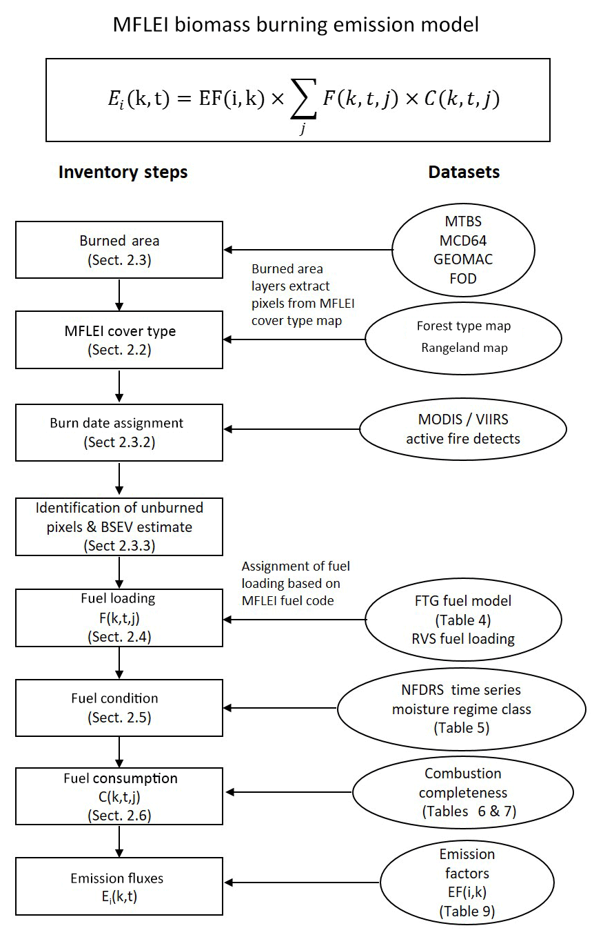
MFLEI provides estimates of daily emissions of CO₂, CO, CH₄, and PM_2.5 from wildland fires for CONUS. The MFLEI biomass burning emission model is based on Eq. (1), given below, and the implementation and datasets are summarized in Fig. 1. The inventory has a spatial resolution of 250 m, which is established by the MFLEI land cover map (Sect. 2.2). Burned pixels are identified and assigned nominal burn dates using a spatially resolved burned area dataset developed from four fire activity datasets (Sect. 2.3). The land cover classifications of the MFLEI map are used to assign fuel loading (biomass per unit area available for combustion) and combustion completeness to burned pixels. Fuel loading of forested pixels is based on a fuel classification system developed from forest inventory measurements (Sect. 2.4.1). A spatially explicit rangeland fuels map supplies fuel loading for pixels of herbaceous and shrub cover types (Sect. 2.4.2). The inventory estimates emission intensities for each 250 m grid cell (k) and day (t) using Eq. (1):

$$\begin{array}{}\text{(1)}& E_i(k,t)=\mathrm{EF}(i,k)\times \sum _{j}F(k,t,j)\times C(k,t,j),\end{array}$$

where E_i is the emission intensity of species i for grid cell k on day t in units of kg i m⁻² day⁻¹. The driving variables in Eq. (1) are the pre-fire dry fuel loading for fuel component j (F; kg m⁻²), combustion completeness, which is the fraction of fuel component j consumed by fire on the day the grid cell burned (C; day⁻¹), and the emission factor for species i, which is the mass of i emitted per mass dry fuel consumed (EF; kg i kg⁻¹). The inventory assumes that the burning and emissions for each burned grid cell occur on the estimated burn day (Sect. 2.3.2). Fuel loading (F), combustion completeness (C), and emission factors (EFs) all depend on grid cell properties. F is assigned based on a grid cell's forest type group or taken from a rangeland fuel loading map in the case of herbaceous and shrub cover types. C depends on fuel type and also on fuel moisture regime and burn severity classification for forest pixels (Sect. 2.6). EFs depend on the fuel type (Sect. 2.7). The mass of species i emitted on the day a grid cell burned (EM_i; kg i day⁻¹) is the product of the emission intensity (E_i) from Eq. (1) and the grid cell area (A), which is 62 500 m².

Table 1 MFLEI cover types and fuel codes.

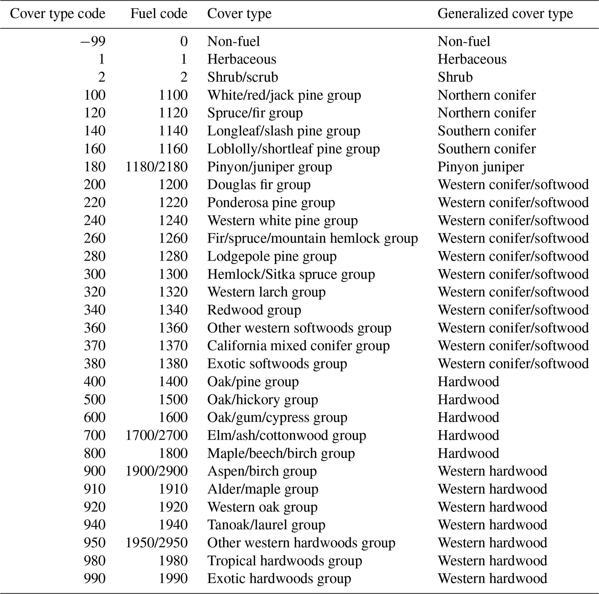
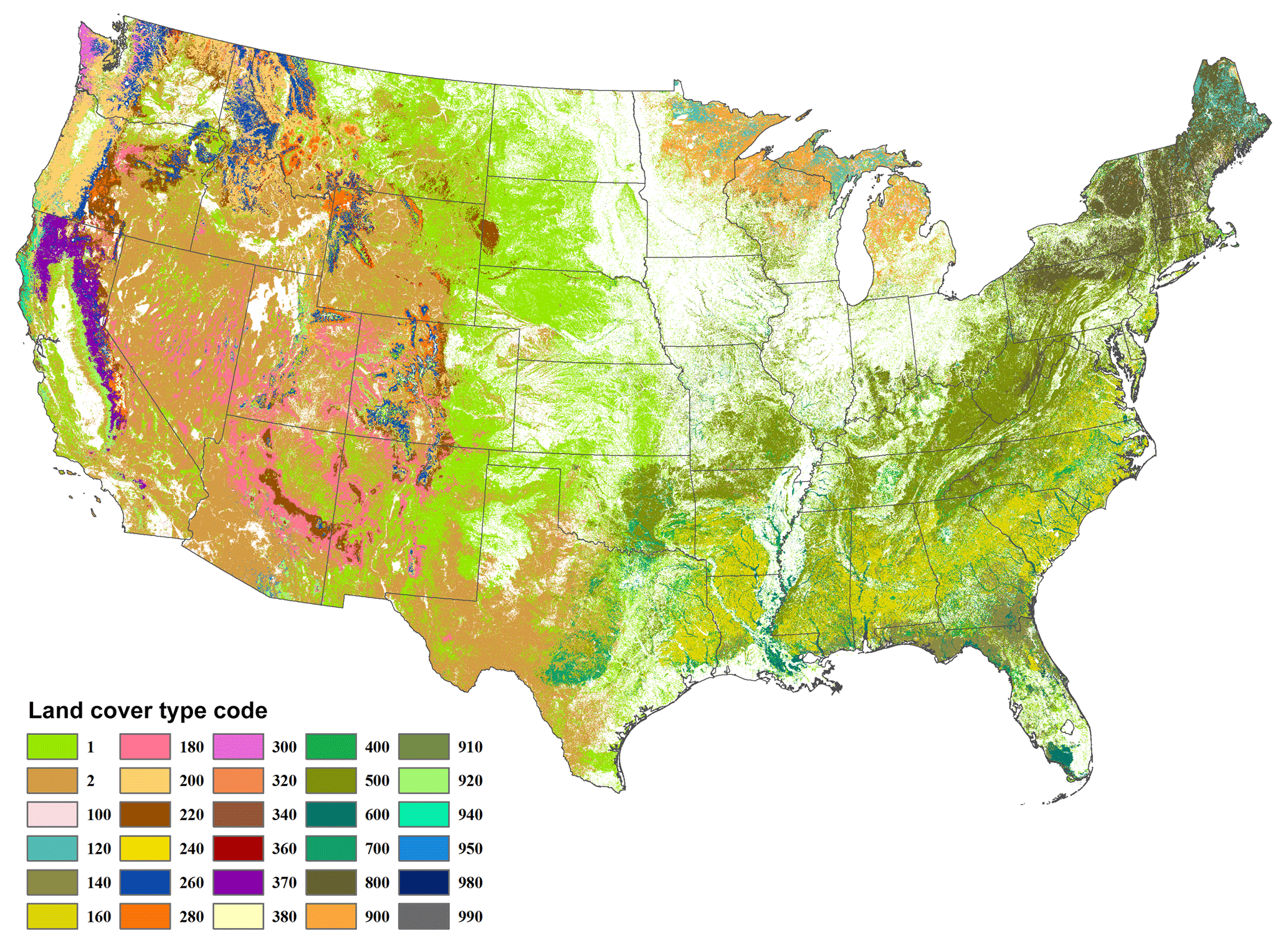
Figure 2 MFLEI land cover type map. White regions indicate the non-fuel cover type. Cover type codes are described in Table 1.

2.2 Land cover map

The MFLEI land cover map was created by combining a 250 m spatial resolution CONUS forest type group map with a rangeland map. The forest type group map, the USDA Forest Service (USFS) National Forest Type Dataset (Ruefenacht et al., 2008; available at https://data.fs.usda.gov/geodata/rastergateway/forest_type/), was used as the base map for the MFLEI land cover map. The forest classification accuracy of the USFS forest type group map is generally around 60 % to 70 % (Keane et al., 2013; Ruefenacht et al., 2008) with a forest/non-forest classification accuracy ranging from 80 % to 98 % (Blackard et al., 2008). Pixels mapped as non-forest in the forest type group map were then assigned a shrub, herbaceous, or non-fuel cover type using the CONUS rangeland product of Reeves and Mitchell (2011). The MFLEI cover type map is shown in Fig. 2 and the cover type descriptions are provided in Table 1. The LANDFIRE project (LANDFIRE, 2016) provides CONUS-wide maps for Fuel Characteristics Classification System (FCCS; Ottmar et al., 2007; McKenzie et al., 2012) and fuel loading models (FLMs; Lutes et al., 2009) fuelbed models, both of which are suitable for estimating fuel consumption and emissions. FCCS is used in both the National Emissions Inventory (NEI) (Larkin et al., 2014) and WFEIS (French et al., 2014) CONUS fire emission inventories. We assembled a new map based on the USFS forest type group map because it provides three important benefits over other land cover maps with respect to forests. First, the accuracy of the forest type group map is significantly better than either the FCCS or FLM maps (Keane et al., 2013). Second, it enabled us to use the fuel type group (FTG) surface fuel classification system (Sect. 2.4.1) which provides a more accurate estimate of average surface fuel loading than either the FCCS or FLM (Keane et al., 2013). Finally, because the USFS forest type group classification is an FIA plot variable, we are able to use the large (>27 000 plots) dataset of FIA fuel measurements estimate uncertainty in surface fuel loading and emissions (Sect. 2.9). During burned area mapping (Sect. 2.3.1), the land cover type codes of the MFLEI are used to assign the fuel codes listed in Table 1 to burned pixels. Three of the mapped cover types were forest type groups for which there was insufficient data to develop a fuel loading classification (Sect. 2.4.1). Therefore, during the burned area processing, the fuel codes associated with these cover types, 1380, 1980, and 1990, were recoded as 1360, 1950, and 1950, respectively. Also, during processing of the burned area data, the fuel codes of forest pixels in the eastern US that were classified as 1180, 1700, 1900, and 1950 were recoded to 2180, 2700, 2900, and 2950, respectively. This was done because the forest inventory surface fuel dataset used to develop fuel classifications (Sect. 2.4.1) indicated substantially different fuel loadings between eastern and western (11 western states) forests for these forest type groups. Burned grid cells classified as non-fuel in the land cover map were assigned a fuel load of 0 and did not produce emissions. In post-emission processing of the dataset, the non-fuel, zero-emission burned pixels were assigned a cover type classification from the National Land Cover Database 2011 (NLCD) (Homer et al., 2015). This was done to track wildfire impacts on agricultural and developed lands or identify possible agricultural burning. Pixels that were not classified as forest or rangeland in the MFLEI land cover map were fixed as “no data” when the NLCD dataset classification was forest, herb, or shrub.

The focus of MFLEI is wildfires, which are fires resulting from unplanned ignitions (e.g., lightning, arson, accidents). The other types of open biomass burning common in CONUS are prescribed fires and agricultural fires. We define agricultural fires as the burning of crop residue or preparation of fields for planting. Croplands are classified as non-fuel in the MFLEI land cover map and are assigned zero emissions in the inventory. Prescribed fires are intentionally ignited to achieve land management objectives (e.g., hazardous fuel reduction, ecosystem restoration, and preparation of rangeland for grazing). Prescribed fires are not excluded from MFLEI, although given the focus on wildfires, they are certainly underrepresented, as discussed in Sect. 3.5.

2.3 Burned area

Burned area was derived from MODIS- and Landsat-based burned area products, a dataset of fire perimeter polygons mapped to support fire management activities, and a fire occurrence database. Burn dates were primarily assigned based on the MODIS burned area product and active fire detection products from MODIS and the Visible Infrared Imaging Radiometer Suite (VIIRS). When a burn date could not be assigned from MODIS or VIIRS data, it was estimated from generalized fire activity cycles and the fire size and duration obtained from the fire occurrence database or other administrative records.

2.3.1 Burned area mapping

On an annual basis, potentially burned grid cells of the MFLEI land cover map were identified by an overlay of burned area polygons and rasters in ArcMap. Four burned area/fire activity datasets were used to extract potentially burned pixels: Monitoring Trends in Burn Severity (MTBS) fire boundaries (MTBS, 2017a; Eidenshink et al., 2007), the MODIS active-fire-based Direct Broadcast Monthly Burned Area Product MCD64A1 (MCD64) (MCD64A1, 2016; Giglio et al., 2009), incident fire perimeters from the Geospatial Multi-Agency Coordination wildland fire support archive (GEOMAC, 2015), and a spatial wildfire occurrence database (FOD) (Short, 2017).

The MTBS project maps fire boundaries and burn severity for large fires (>404 ha in the west and >202 ha in the east) across the US from 1984 to the present (Eidenshink et al., 2007; MTBS, 2017c). MTBS fire boundaries are polygons representing burned area detected from post-fire Landsat Thematic Mapper/Enhanced Thematic Mapper/Operational Land Imager (TM/ETM/OLI) imagery (Eidenshink et al., 2007). The polygon attributes for each MTBS boundary include a unique fire ID, fire start date, and fire name. The MTBS fire ID attribute was used to aggregate burned grid cells by fire events and to filter the FOD point dataset to avoid double counting of fires. The primary MTBS product is thematic burn severity rasters, which classify burn severity within the fire boundaries (Eidenshink et al., 2007; MTBS, 2017b). We used the MTBS burn severity rasters to identify unburned regions within MTBS fire boundaries and to develop scaling factors to approximate unburned patches for burned area mapped using MCD64, GEOMAC, and FOD, as described in Sect. 2.3.3.

The MCD64 product maps burned areas using 500 m MODIS imagery coupled with 1 km MODIS active fire detections (Giglio et al., 2009). MCD64 is a monthly 500 m resolution raster product that provides an estimated burn date for each pixel identified as burned. We used MODIS Collection 5.1 of MCD64A1 (MCD64A1, 2016). The most recent version of the MCD64A1 product, Collection 6, became available in January 2017 (Giglio et al., 2015). The MCD64 product is the primary burned area data source for the Global Fire Emission Database (GFED) (Giglio et al., 2013) during the MODIS era. Details for accessing the product can be found on the GFED website: http://www.globalfiredata.org/ (last access: 4 June 2018).

The GEOMAC dataset is a collection of fire perimeter polygons. For large fire events, fire perimeters are periodically mapped by incident management teams, typically using airborne infrared imagery. These incident perimeter polygons are produced to support fire management activities. Since their purpose is identifying the fire perimeter, not mapping the actual area burned, the area within a perimeter typically includes unburned regions. We attempt to compensate for this as discussed in Sect. 2.3.3. For these reasons, we give the MTBS dataset precedence over the GEOMAC. Further discussion regarding the use of incident perimeters as “ground-truth” burned area may be found in Urbanski et al. (2009) and Key and Benson (2006). Final fire perimeters from the GEOMAC dataset were checked against the MTBS fire boundaries using the products' fire name attributes to remove GEOMAC perimeters for fires present in the MTBS dataset.

FOD is a spatial database of wildfires that occurred in the United States from 1992 to 2015 generated from wildfire records acquired from the reporting systems of federal, state, and local fire organizations (Short, 2017). FOD provides a point location for each fire, not a spatial object that maps burned area. Other FOD dataset attributes used in our analysis include final fire area, discovery date, containment date, fire name, fire code, and the MTBS fire ID attribute from the MTBS perimeter dataset (MTBS fires only). We used the FOD dataset to capture fires not included in the MTBS, GEOMAC, or MCD64 datasets. We filtered the FOD dataset for fires contained in either the MTBS or GEOMAC datasets using the MTBS fire ID or the fire name and fire code attributes (for GEOMAC) from the datasets. Fires <4 ha in size were also removed due to their minor contribution to total burned area, while fires <4 ha accounted for 86 % of all fires in the FOD database for 2003–2015, they only comprised 1.5 % of total fire area. Finally, FOD fires with locations that fell within a distance D_f ($D_{\text{f}}=\mathrm{2}\sqrt{A}/\mathit{\pi }$, where A is the FOD fire area) of any grid cell identified as burned by either the MCD64 or GEOMAC datasets were removed. Following these filtering actions, MFLEI land cover map grid cells within a distance D_f∕2 of the FOD fire location were flagged as burned.

2.3.2 Burn date assignment

Of the four datasets used to map burned area, only MCD64 provides an estimated burn date, and these were assigned to MFLEI grid cells identified as burned by the MCD64 product. Grid cells identified as burned by the MTBS, GEOMAC, or FOD datasets were assigned an estimated burn date as follows. First, all (non-MCD64-sourced) grid cells were assigned a fire start date and, when available, a fire containment date, on a fire event basis. The MTBS, GEOMAC, and FOD datasets include fire event identifiers and fire start dates (or discovery dates) which were added as attributes to burned grid cells. The FOD dataset also includes a containment date for many fire events and it was added as an attribute to burned MFLEI grid cells when available. Most of the fires in the MTBS and GEOMAC dataset are also included in FOD. Fire event identifiers, MTBS Fire ID, and the fire name and fire code attributes from GEOMAC, were used to associate MTBS- and GEOMAC-sourced burned pixels with FOD fire events and thereby assign containment dates when available. Next, grid cells identified as burned by the MTBS, GEOMAC, or FOD datasets were assigned an estimated burn date using one of the following methods in order of precedence:

1. Grid cells within 500 m of a MCD64-sourced pixel were assigned that pixel's burn date.

2. Grid cell burn dates were assigned from MODIS active fire detections (MCD14) (Giglio et al., 2003) using spatial and temporal proximity criteria to associate active fire detections with burned grid cells. We assigned each active fire detection a spatial buffer, X_b, which defines the maximum distance at which it can be associated with a MFLEI grid cell for purposes of ascribing a burn date. MCD14 pixels have nominal dimensions of 1 km × 1 km; however, the actual size and location of a detected active fire are unknown. In consideration of this spatial uncertainty, we assigned X_b a default value of 2 km. The dimensions of MCD14 pixels are 1 km × 1 km at nadir but increase with distance off nadir, reaching 4.8 km (scan direction) × 2 km (track direction) on the edges of the MODIS scanning swath (Nishihama et al., 1997). For off-nadir pixels, X_b was set to the dimension of the scan direction when >2 km (pixel dimensions were among the attributes of the MCD14 product used in analysis). For each burned grid cell, we identified the nearest active fire detection located within a distance X_b and falling in the time frame (D_start−3 days) to (D_cont+3 days), where D_start and D_cont are the grid cell's fire start date and fire containment date attributes. The temporal criteria were used to eliminate any active fire detections from an unrelated fire that occurred during a different time period. For the years 2014 and 2015, VIIRS I-band active fire detections (Schroeder et al., 2014) were also used to assign pixel burn dates. The procedure was similar to that used with the MCD14 product, except that the VIIRS active fire detection spatial buffer, X_b, was set to 750 m, which is twice the spatial resolution (375 m) of VIIRS I-band pixels at nadir. Because the VIIRS I-band active fire detection product has significantly superior mapping capabilities compared to the MCD14 product (Schroeder et al., 2014), it was given precedence over MCD14 for assigning pixel burn dates. Burned grid cells not associated with MCD64 were assigned a burn date equal to the date of the nearest active fire detection meeting the above spatial and temporal criteria. The MCD14 and VIIRS I-band active fire data used were obtained from the USDA Forest Service Remote Sensing Application Center's Active Fire Mapping Program (https://fsapps.nwcg.gov/afm/gisdata.php, last access: 10 April 2017, USDA Forest Service, 2017).

3. For event-based extrapolation, following burn date assignment steps 1 and 2, 28 % of the burned grid cells were without burn dates. Overall, 46 % of these undated grid cells were associated with fire events which had some grid cells that did have burn dates. For these fire events, grid cells without burn dates were assigned the burn date of the nearest grid cell with a burn date.

4. The final step for assigning burn dates addressed burned grid cells of “dateless” fire events, those without any burn date associated with the grid cells. In order to assign estimated burn dates to these grid cells, which comprised 15 % of all the grid cells, we developed what we refer to as “burn-day distributions”. These are empirical distributions of the fraction of event total burned area as a function of days since ignition. One set of burn-day distributions was derived using MTBS fire events which had a containment date and also had >95 % of grid cells assigned a burn date in steps 1 or 2 above. From these fire events, burn-day distributions were created according to six fire size classes (in hectares): 200–625, 625–1250, 1250–3125, 3125–6250, 6250–12 500, and 12 500–25 000. The burn-day distribution for the 12 500–25 000 ha size class is shown in Fig. A1, and the distributions for all six size classes are provided in the Supplement dataset (file\Supplements\BurnDayDist.csv; see Sect. 4). The burned grid cells of dateless fire events >200 ha in size were assigned burn dates using the burn-day distribution for the appropriate size class. For fire events with a containment date, the burn-day distribution was truncated to correspond to the fire duration (containment date – fire start date) and normalized. When a dateless fire event was <200 ha and had a containment date, grid cell burn dates were assigned one at time cycling through the days between the fire start date and the containment date in chronological order until all grid cells were assigned. Fire events <200 ha and without containment dates were assigned durations using Table A1, and the burned grid cells were distributed one per burn day by cycling through the burn days in chronological order until all grid cells were assigned.

2.3.3 Unburned and lightly burned grid cells

Wildfires typically do not impact fuels uniformly across the landscape and it is not unusual for significant area within a fire perimeter to be unburned or only lightly burned (Kolden et al., 2012). MTBS burn severity thematic classifications were used to account for unburned or lightly burned regions (MTBS, 2017b). The MTBS burn severity thematic classifications were developed to represent fire effects on aboveground biomass (Eidenshink et al., 2007; Schwind, 2008). MTBS assigns six burn severity classifications (BSEVs) to pixels within fire boundaries: (1) unburned to low burn severity, (2) low burn severity, (3) moderate burn severity, (4) high burn severity, (5) increased green, and (6) no data. We elected to designate a BSEV 1 as unburned, which is consistent with MTBS program publications that describe this classification as areas which are either unburned or where visible fire effects occupy <5 % of the site at the time of observation (Schwind, 2008). The increased green classification may indicate unburned areas that exhibited more green at the time of the post-fire Landsat scene relative to the pre-fire scene. The increased green classification was assigned to just 0.3 % of MTBS pixels and thus has a negligible impact on our inventory. MFLEI burned grid cells associated with a fire analyzed by the MTBS project were compared against a coarse-scale MTBS thematic burn severity map (30 m original resampled to the MFLEI 250 m grid using majority sampling). Coarse-scale MTBS pixels classified as BSEV 5 or BSEV 6, increased green or no data, respectively, were randomly reassigned a value between 1 and 4. This reassignment was conducted on a fire event basis in proportion to the frequency of pixels originally classified BSEVs 1–4. MFLEI grid cells classified as BSEV 1, “unburned to low severity”, in the coarse-scale MTBS product were flagged as unburned. MFLEI burned grid cells not associated with a fire analyzed by the MTBS project were randomly assigned a BSEV value based on a generic cover type–BSEV empirical distribution developed from the CONUS-wide MTBS thematic classification maps for 2003–2013. The cover type–BSEV distribution is shown in Table 2.

Table 2 MTBS burn severity class percent distribution by generalized cover types for 2003–2013.

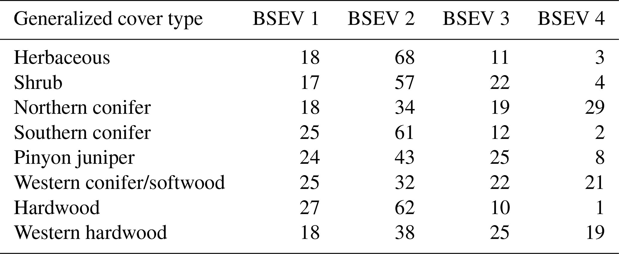
Table 3 Description of fuel components.

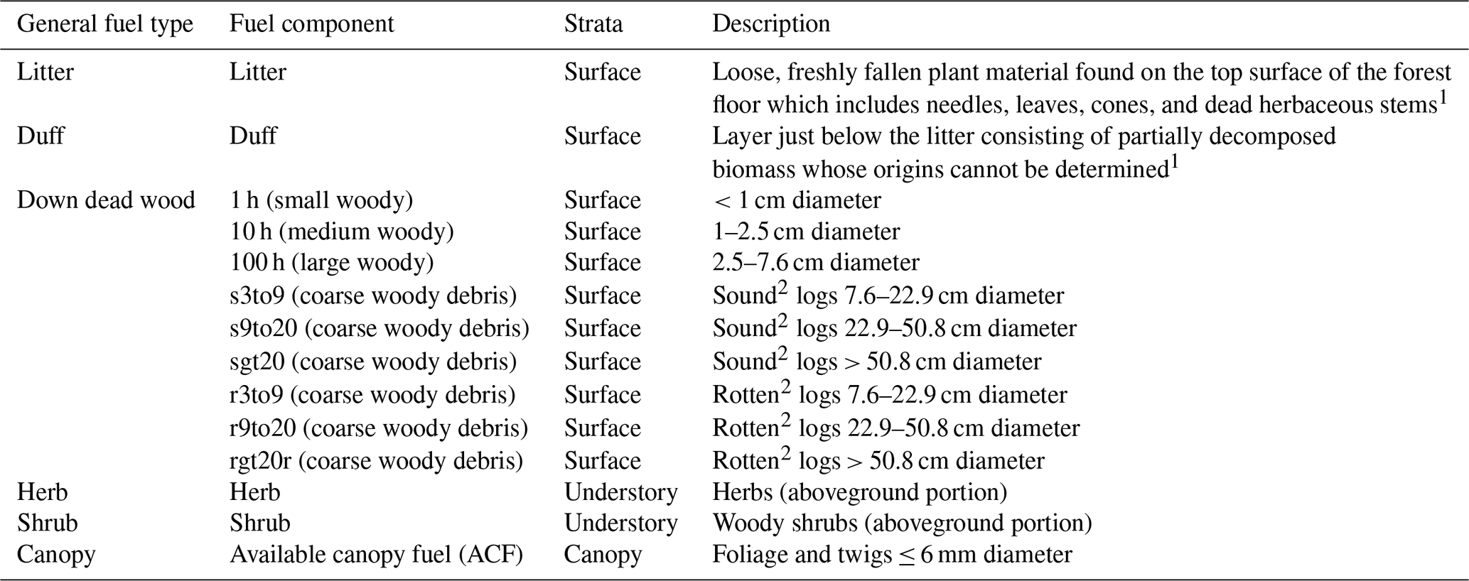
¹ O'Connell et al. (2016). ² Sound logs are logs assigned FIA decay classes 1, 2, or 3, and rotten logs are logs assigned FIA decay class 4 or 5 (O'Connell et al., 2016).

2.4 Fuel loading

Fuel loading was represented with the 14 fuel components in Table 3. Models of forest fuel loading were developed using data from the USFS Forest Inventory and Analysis (FIA) National Program as described in Sect. 2.4.1. The rangeland fuel product (Sect. 2.4.2) provided spatially explicit fuel loadings for grassland and shrub ecosystems.

Figure 3 Location of FIA plots used to develop surface fuel loading classifications.

2.4.1 Forest fuel loading

Surface fuel loadings

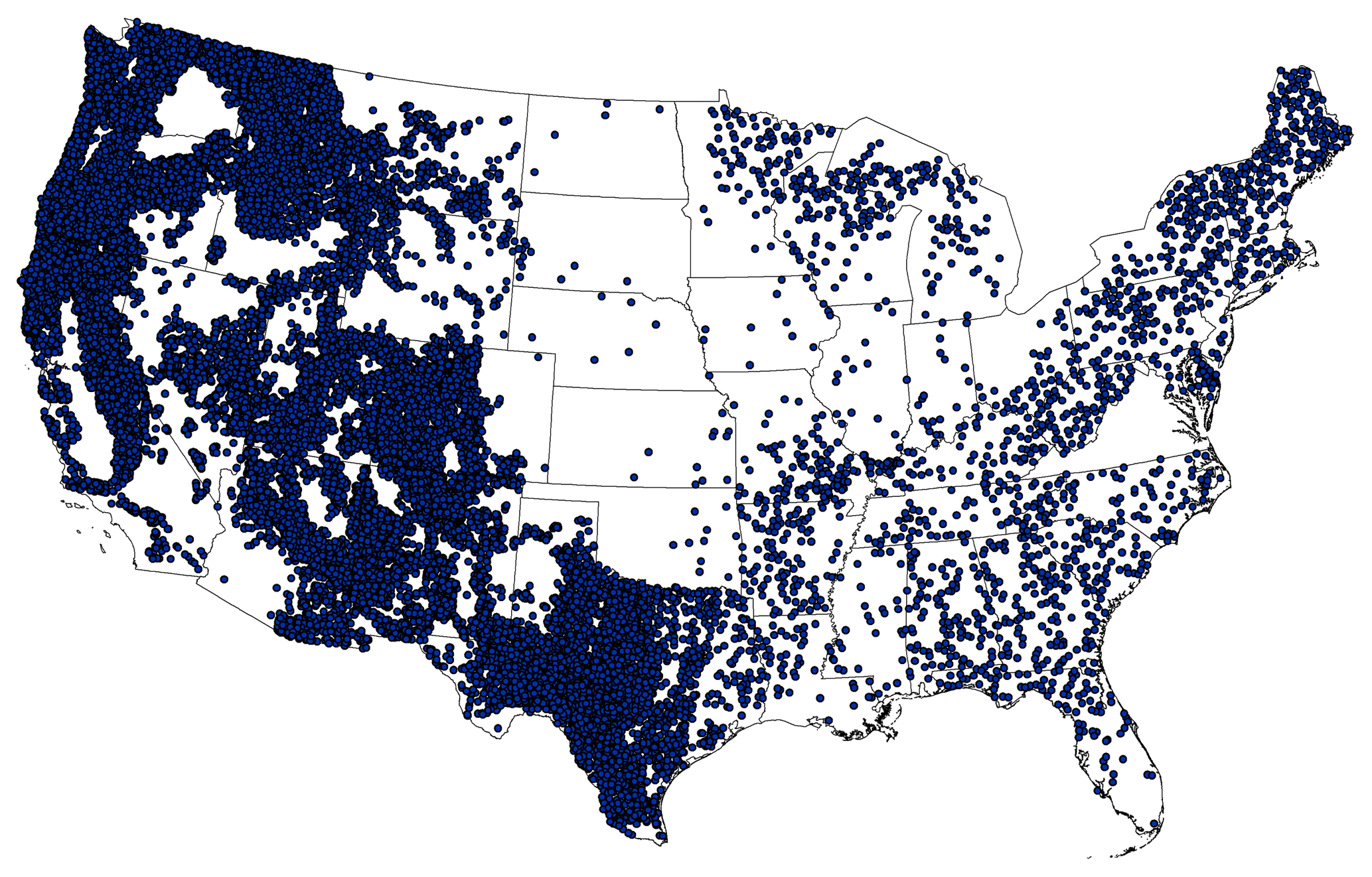
We developed an expanded version of the FTG fuel classification system assembled by Keane et al. (2013) using recently available FIA fuel data and also including plot data from the eastern US. The FIA inventory is comprised of three phases of data collection, as described in Bechtold and Patterson (2005). The inventory is designed to cover forested land (10 % stocked with tree species; see Bechtold and Patterson, 2005) of all ownership across the US. Phase 1 sampling provides information to stratify inventory ground plots and improve the precision of estimates of population totals (Bechtold and Patterson, 2005). In phase 2, measurements are taken on the standard FIA base grid, which has a density of approximately one sample location per ∼2428 ha (6000 acres). Phase 2 collects information such as height and diameter of standing trees and physiographic class and land ownership. Phase 3 involves sampling of forest health indicators, such as the down woody material (DWM) indicator. The DWM indicator estimates dead organic materials including downed woody debris, litter, and duff (Woodall and Monleon, 2008). The DWM indicator was used to estimate plot-level surface fuel loading as described below. Phase 3 sampling is conducted on a subset of phase 2 plots (approximately 1∕16 of phase 2 plots). In the western US, the FIA units began collecting the DWM indicator on all of their phase 2 plots in the early 2000s (Keane et al., 2013); thus, the density of surface fuel plots used to assemble the FTG classification is significantly higher in the west. Figure 3 maps the locations of the FIA plots used to develop the expanded FTG surface fuel classification for MFLEI.

Table 4 Fuel loading (kg m⁻²) by fuel component for the FTG classification. Litter and duff depth are in centimeters. See Table 3 for descriptions.

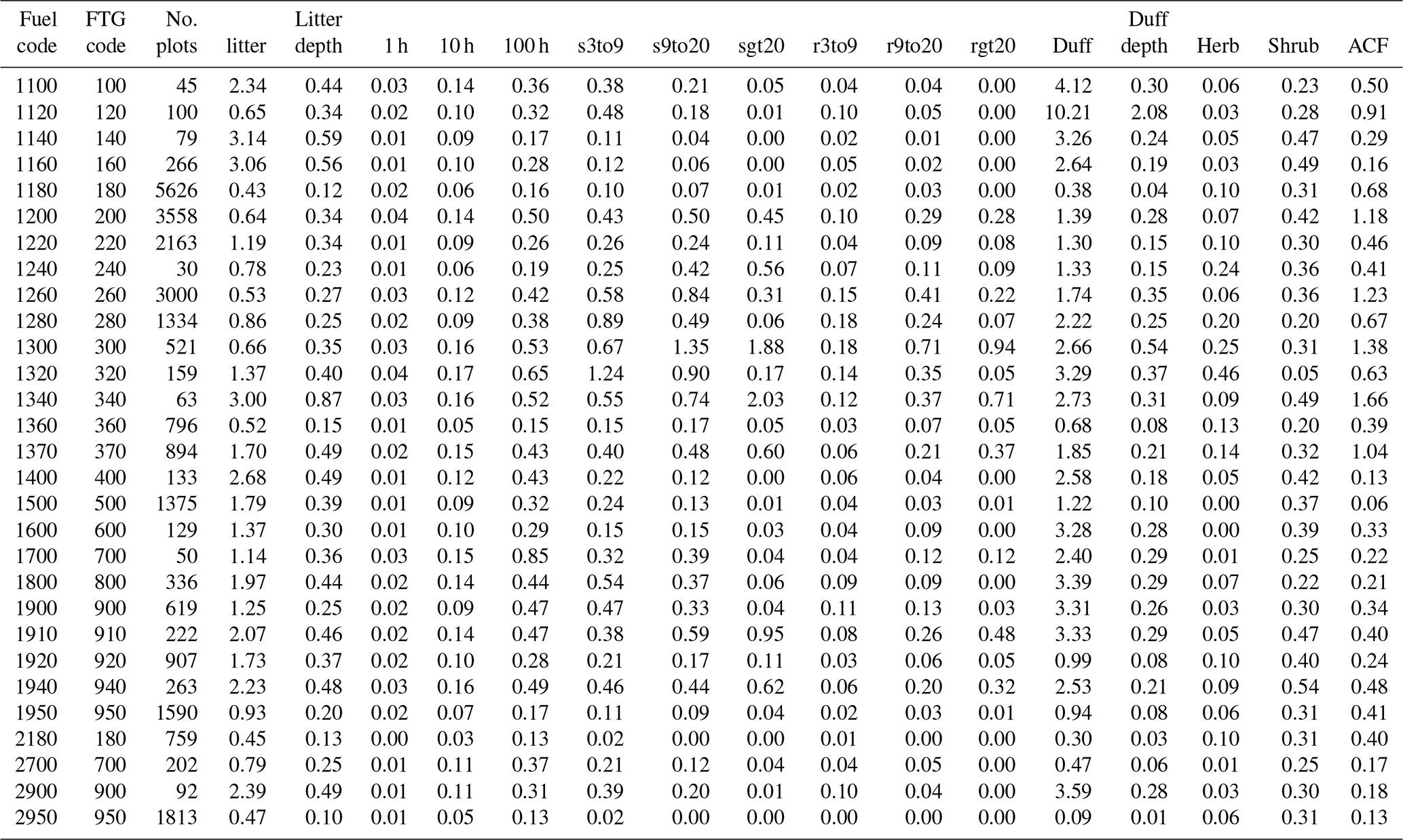
Our FTG classification is based on 27 124 plots compared with 13 138 used in Keane et al. (2013). We used only single condition plots, plots where all four subplots were the same condition (land class, reserved status, owner group, forest type, stand-size class, regeneration status, and stand density) (O'Connell et al., 2016). The FTG classification summarizes fuelbed component loadings (Table 3) by FIA forest type groups using fuel data from the FIA database acquired from the FIA DataMart website (https://www.fia.fs.fed.us/tools-data, last access: 10 April 2017; FIA, 2015). Five tables were accessed from the FIA dataset: REF_FOREST_TYPE, COND, PLOT, COND_ DWM_CALC, and DWM_COARSE_WOODY_DEBRIS. A detailed description of these tables is provided by O'Connell et al. (2016). For an in-depth description of the FIA sampling design, estimation, and analysis procedures, see Woodall and Monleon (2008), O'Connell et al. (2016), and Woodall et al. (2013), and for an abbreviated summary, see Keane et al. (2013). Data assembled from the COND_DWM_CALC table included loading (biomass per unit area) of fine woody debris by three size classes: small, medium, and large (Table 3); duff loading and depth; and litter loading and depth. Data from the DWM_COARSE_WOODY_DEBRIS table were assembled to provide loadings of coarse woody debris by eight size/decay class combinations (Table 3) following the methods described in Woodall and Monleon (2008). Best-estimate loadings of the surface fuel components were taken as the average values of all plots for each fuel classification and are shown in Table 4. The surface fuel loading data for the 27 124 plots used to develop Table 4 and to derive uncertainty estimates in the emission modeling (Sect. 2.9) are included in the MFLEI dataset (file\Supplements\Fuel_Load_Plot_Data.csv; see Sect. 4). The MFLEI land cover type map assigns an FTG to all forest pixels. Four FTGs (180, 700, 900, and 950) had significant fuel loading differences between western (11 western states) and eastern plots. Therefore, separate fuel classifications (west and east) were made for these FTGs and they are differentiated by the fuel code (Table 1) which is assigned during burned area mapping, as described in Sect. 2.2. As discussed in Keane et al. (2013), the variability of surface fuel loading within FTGs is quite large. Figure 4 plots the distribution of surface fuel loading for the FIA plots of three FTGs, loblolly/shortleaf pine (160), Douglas fir (200), and California mixed conifer (370). The surface fuel loading plot data have a lognormal-like distribution with long tails. The high variability in surface fuel loading is the primary source of uncertainty in the emission estimates for forest fires (Sect. 2.9).

Figure 4 The distribution of surface fuel loading for the FIA plots of three FTGs: loblolly/shortleaf pine (160), Douglas fir (200), and California mixed conifer (370).

Understory fuels

The loading of forest understory fuels, shrubs (vascular plants with woody stems that are not defined as trees by FIA phase 2), and herbs (non-woody vascular plants including but not limited to ferns, moss, lichens, sedges, and grasses) was derived from raster maps of forest understory carbon (Wilson et al., 2013). The raster maps of forest understory carbon were combined with the USFS FIA FTG map (Ruefenacht et al., 2008) to derive empirical distributions of understory fuel loading for each FTG class (assuming a biomass carbon content of 50 %). The fuel loading distributions were used to provide uncertainty estimates for the emission modeling (Sect. 2.9). Partitioning of the understory fuel loading between shrubs and herbs was based on herb-to-shrub ratios from the Fuel Characteristics Classification System (FCCS) and First Order Fire Effects Model (FOFEM) reference fuel models (Ottmar et al., 2007; Riccardi et al., 2007; Lutes, 2016a). The empirical distributions of understory fuel loading for all FTG classes are included in the MFLEI dataset (file\Supplements\Understory_Fuel_Dist.csv; see Sect. 4). Best-estimate loadings for herb and shrub fuel components were taken as the average values of all plots for each fuel classification and are shown in Table 4.

Canopy fuels

Available canopy fuel (ACF), the dry mass of canopy fuels likely to be consumed in a fully active crown fire (needles, lichen, moss, and live and dead branch wood ≤6 mm in diameter) (Scott and Reinhardt, 2001), was derived from FIA plot Treelist tables. FIA Treelist tables (which are named TREE in the FIA database) provide a detailed inventory of trees on FIA plots (O'Connell et al., 2017). FIA plots with Treelists are based on phase 2 sampling and are far more numerous than the phase 3 plots used to derive surface fuel loadings (see above). We used the Treelist table variables: species code (SPCD), diameter (D), crown class code (CCLCD), tree status (STATUSCD), and tree density (TPA) to estimate ACF associated with each Treelist table entry using empirical equations from the literature following the approach outlined in the FuelCalc user's guide (Lutes, 2016b). FuelCalc is a fuel management software system which can be used to calculate forest canopy characteristics at an inventory plot. For each of the 363 060 FIA plots with a Treelist, stand-level ACF was calculated using Eq. (2):

$$\begin{array}{}\text{(2)}& {\text{ACF}}_{\text{stand}}=\sum _i^N({\text{acf}}_i\times {\text{TPA}}_i),\end{array}$$

where the subscript i is the index for the softwood tree species in the stand, and acf_i and TPA_i are tree-level available canopy fuel and tree density. acf_i and TPA_i are calculated as described in the Supplement. ACF_stand values were aggregated by FTG (an FIA plot variable) and the mean was taken as the best estimate (listed in Table 4). The ACF_stand values aggregated by FTG were fit to Weibull probability distribution functions to derive uncertainty estimates for the emission modeling (Sect. 2.9). Best-estimate ACF and optimized parameters for fits to Weibull probability distribution functions (PDFs) are provided in Table B1.

Figure 5 Best-estimate (Table 4) forest fuel loading in canopy, understory, and surface fuels by fuel type.

Total forest fuel loading

Average forest fuel loading is dominated by the surface fuels for all forest fuel types (25 FTGs plus four eastern variants; see Sect. 2.2), as shown in Fig. 5. More than 70 % of total fuel loading resides in the surface fuels for 25 of the 29 forest fuel types. Surface fuel components (Table 3) are often grouped into litter, fine woody debris (fwd; down dead wood with diameter < 7.62 cm), coarse woody debris (cwd; down dead wood with diameter >= 7.62 cm), and duff. These groupings reflect the surface-to-volume ratio of the fuel particles, an important determinant in the rate of fire spread (Scott and Burgan, 2005), as well as the combustion characteristic of the fuels. Litter and fine woody debris tend to favor flaming combustion, while coarse woody debris, and duff especially, favor smoldering combustion processes (Urbanski, 2014). Figure 6 plots the fraction of total fuel load residing in duff, litter, fine woody debris, and coarse woody debris for the 29 forest fuel types.

Figure 6 Fraction of best-estimate (Table 4) total forest fuel loading in surface fuel loading groups by fuel type.

2.4.2 Rangeland fuel loading

Rangeland fuels were estimated using the Rangeland Vegetation Simulator (RVS) (Reeves, 2016) and began with delineating the spatial domain of rangeland in CONUS (land cover type codes 1 and 2 in Fig. 2), as described in Reeves and Mitchell (2011), and constrained using the forest type map developed by Blackard et al. (2008). If a forest type was indicated for a given pixel in the Blackard et al. (2008) map, no rangeland fuel data were estimated for that pixel. The vegetation form (herbaceous or shrub) and type (e.g., Chihuahuan mixed desert and thorn scrub) were assigned from the LANDFIRE (LF) project existing vegetation type (EVT) geospatial data layer (LANDFIRE, 2016). Different methods were used to quantify woody and herbaceous fuels (Fig. 7).

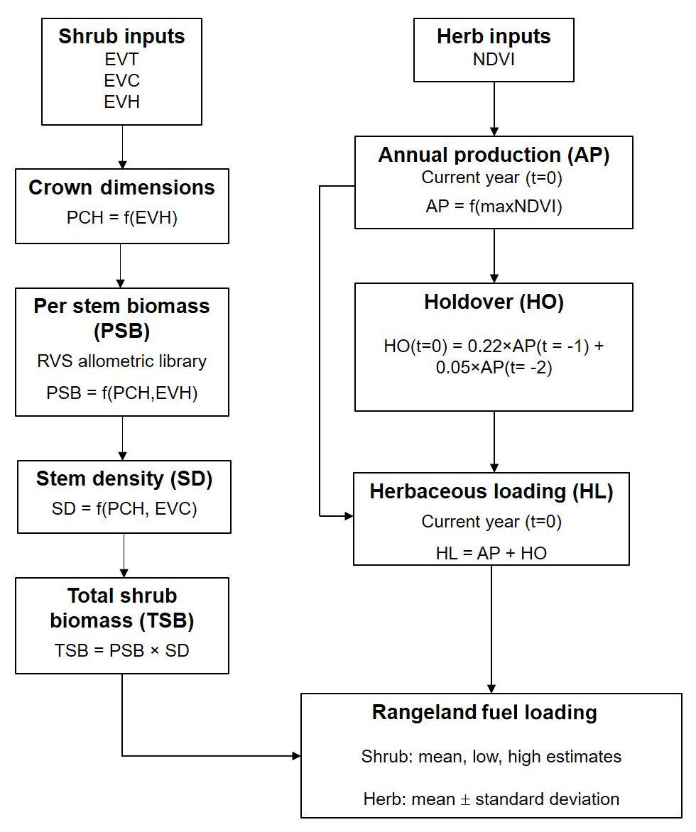
Figure 7 Abbreviated flow of data and actions in RVS to produce rangeland fuel loadings. EVT, EVC, and EVH are existing vegetation type, existing vegetation cover, and existing vegetation height from the LANDFIRE project.

Shrub

The derivation of shrub fuel loading used two LF products in addition to EVT as input: existing vegetation height (EVH) and existing vegetation cover (EVC). The height estimates at each pixel in the EVH product are thematic classes representing a range of potential heights (Table C1). The range of potential heights provided by the EVH enables three values of shrub fuels to be estimated at each pixel (median, maximum, and minimum). EVC represents the vertically projected percent cover of the live canopy.

Generation of shrub fuel loading data involves several steps (Fig. 7) which are briefly described here. Details of the approach are illustrated in Appendix C. First, crown dimensions are derived from EVH and the projected crown area on a horizontal surface (PCH), the latter of which is estimated using Eq. (3) (Frandsen, 1983):

$$\begin{array}{}\text{(3)}& {\log }_{\mathrm{10}}\left(\mathrm{PCH}\right)=-\mathrm{0.8471}+\mathrm{2.2953}{\log }_{\mathrm{10}}\left(\text{HT}\right),\end{array}$$

where PCH is in cm² and HT is the estimated height class of shrubs in centimeters at each pixel (from the EVH product). Crown dimensions are then used in one of 31 species-specific equations from the RVS allometric library to estimate per stem biomass (PSB; kg stem⁻¹). Next, the estimate of stem density (SD) at each pixel (stem ha⁻¹) is used to expand PSB to a per area basis. SD is estimated as

$$\begin{array}{}\text{(4)}& \text{SD}=(\text{PCH}/{\mathrm{10}}^{\mathrm{8}})\times \text{EVC},\end{array}$$

where SD is stem density, and the value 10⁸ cm² converts to a per hectare basis. In effect, the number of times PCH can be divided into a hectare is scaled by the canopy cover (EVC). The total shrub biomass (TSB; kg ha⁻¹) is the product of PSB and SD. This four-step process was conducted at each pixel using the minimum, maximum, and median shrub heights from EVH (Table C1) to provide lower, upper, and middle estimates of fuel loading, respectively.

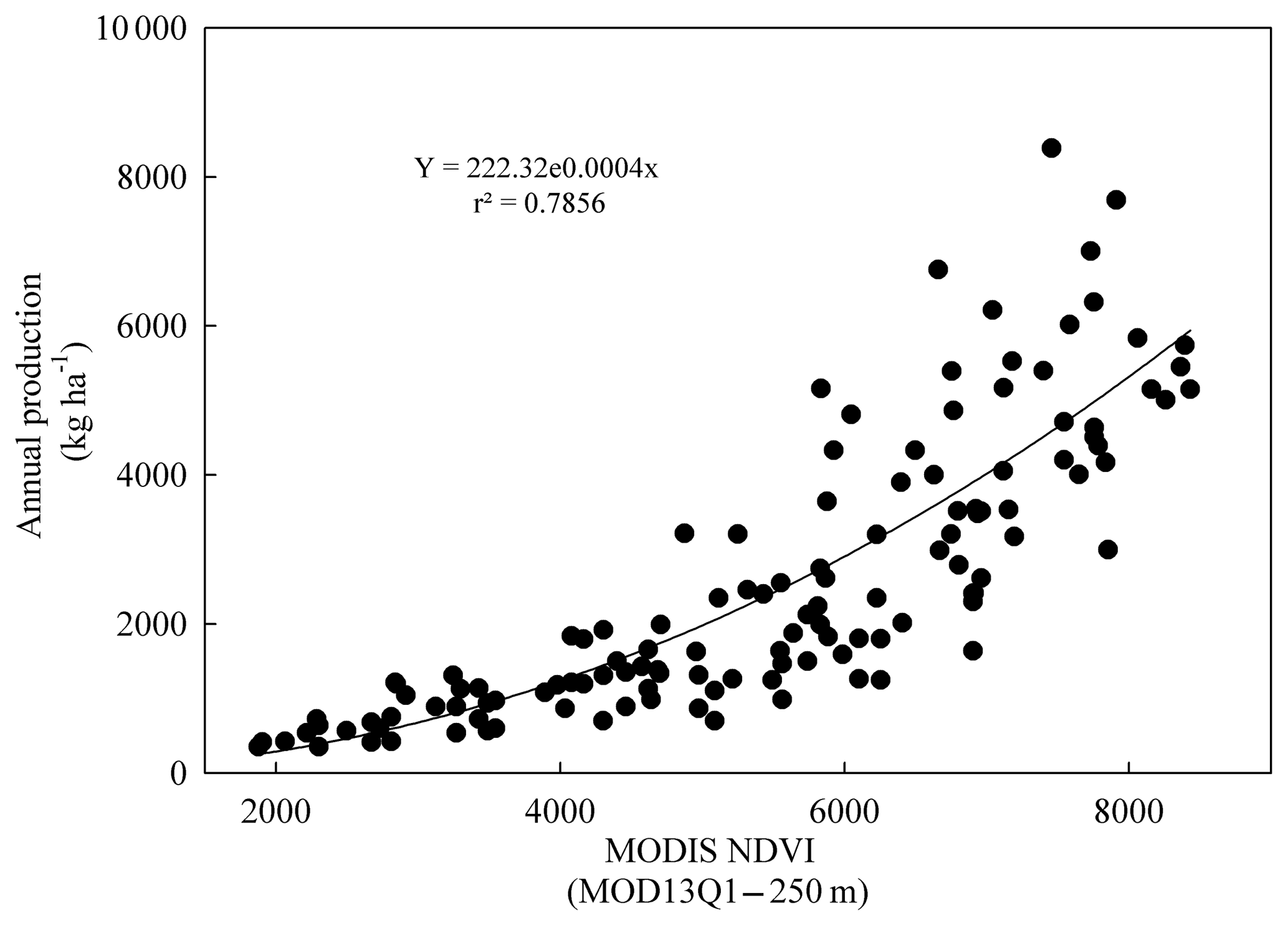
Figure 8 Relationship between annual production and annual maximum Normalized Difference Vegetation Index (NDVI) on 51 grassland vegetation types.

Herb

The derivation of herb fuel loading used the EVT and MODIS growing season maximum Normalized Difference Vegetation Index (NDVI) and the Soil Survey Geographic (SSURGO) annual productivity map, which consists of polygons with estimates of rangeland productivity (dry weight/area/year) for normal, favorable, and unfavorable production years (Soil Survey Staff, 2016). The SSURGO productivity data were derived from the USDA National Resource Conservation Service soil survey geographic database (Soil Survey Staff, 2016). Herbaceous biomass is estimated as a function of the annual maximum NDVI across 51 grassland vegetation types. The three SSURGO production values reported at each soil polygon were paired with the average, minimum, and maximum NDVI values (from 2000 to 2016) for each of the 51 vegetation types dominated by herbaceous species (Fig. 8). When this relationship is applied for each year in the time series between 2000 and 2016, an annual estimate of rangeland production can be made at every pixel. The present year's herbaceous production (from 2000 to 2016) is added to estimated standing dead herbaceous vegetation (“holdover”) resulting from previous growth (see below). Annual production added to the holdover from previous years creates the “herbaceous loading” (HL; Fig. 7) pool.

Estimating the previous year's standing dead or herbaceous litter material is based upon experimental (Irisarri et al., 2016) and anecdotal observations. This topic is not widely studied across multiple ecosystems and it is difficult and time consuming to derive experiments that track the fate of herbaceous growth, senescence and decomposition across multiple vegetation types. The paucity of suitable plot data for estimating the amount of standing dead material is therefore based on observations of various vegetation stands with significant herbaceous components throughout the western US. In addition, the USDA Agricultural Research Service (ARS) recently provided results from 10 years of grassland observations on shortgrass steppe near Cheyenne, Wyoming, and standing dead values averaged 22 % across treatments. This means that, on average, in shortgrass steppe, standing crop of the present year includes 22 % of the previous year's production plus the present annual production. The function used in the RVS to estimate the standing dead material is $y=\mathrm{100}{e}^{-\mathrm{1.495}x}$, which yields values of 22 % at year 1 and 5 % at year 2.

To capture the range of variability of the herbaceous response, the coefficient of variation (C.V. is the mean divided by the standard deviation of the annual production between 2000 and 2016) was applied at each pixel dominated by herbaceous life forms. This yields three potential values of herbaceous loading at each pixel (mean, mean ± C.V.). Likewise, the range of standing dead values over 2000–2016 was estimated using the mean ± C.V. At this stage, HL and total shrub biomass loading (TSB) have been produced and are mosaicked together to form a seamless depiction of fuels and are available for simulation of fuel consumption and emissions. Raster files of the herbaceous C.V. and the shrub minimum and maximum are included in the MFLEI dataset.

Figure 9 Map of best-estimate fuel loading for forest and rangeland in g m⁻².

2.4.3 Total fuel loading

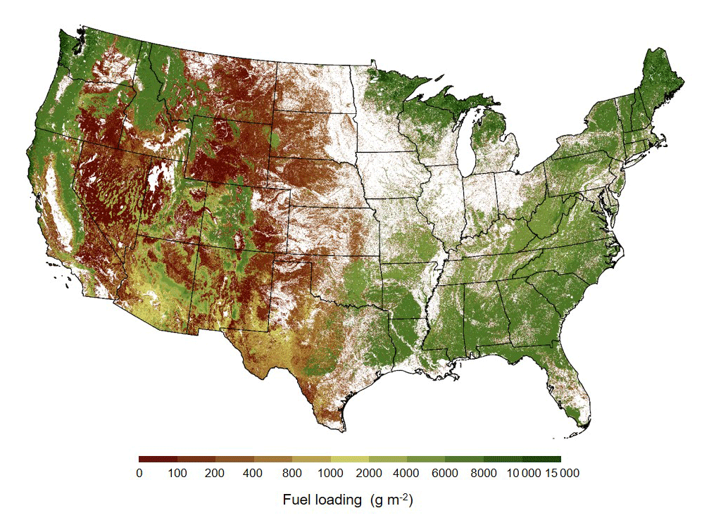
Best-estimate total fuel loading of both forests and rangeland are mapped in Fig. 9. Forest fuel loadings range from 1.3 to 13.3 kg m⁻² (Table 4, Fig. 5). Fuel loadings are considerably less for rangeland, varying from ∼0.1 to 5.2 kg m⁻², with a median value of 1.8 kg m⁻². Regions without a mapped fuel loading are classified as non-fuel and are largely agriculture, barren, developed lands, or water.

2.5 Fuel conditions

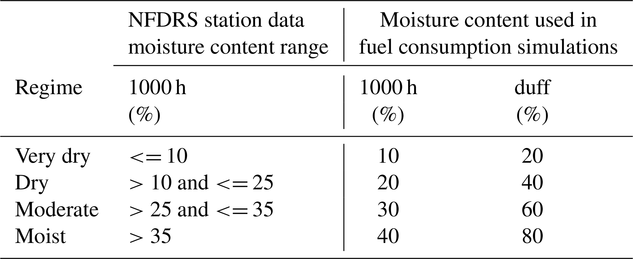
Fuel moisture content is a key driver of fuel consumption, especially for coarse woody debris and duff. The National Fire Danger Rating System (NFDRS; Cohen and Deeming, 1985) provides fuel moisture models that classify dead fuels by time lag intervals which are proportional to the fuel particle diameter. The NFDRS classifications for dead fuel moisture are 1, 10, 100, and 1000 h corresponding to diameters of <0.64, 0.64–2.54, 2.54–7.62, and >7.62 cm. The algorithms used to simulate surface fuel consumption require fuel moisture content for 1000 h time lag fuels and duff. Surface fuel consumption was simulated for the four fuel moisture regimes shown in Table 5. In the emission modeling, MFLEI grid cells were assigned the 1000 h time lag or 100 h time lag fuel moisture content of the nearest NFDRS station for the day of concern. The 1000 h fuel moisture content is considered a proxy for coarse woody debris (see Table 3). Data for NFDRS stations were obtained from the USFS Wildland Fire Assessment System (WFAS) (USDA Forest Service, 2015) data archive. Missing values were filled by linear interpolation across days. Duff moisture content was estimated using the 100 h fuel moisture content and empirical relationships of Harrington (1982).

Table 5 Fuel moisture regimes used for simulating fuel consumption.

2.6 Fuel consumption

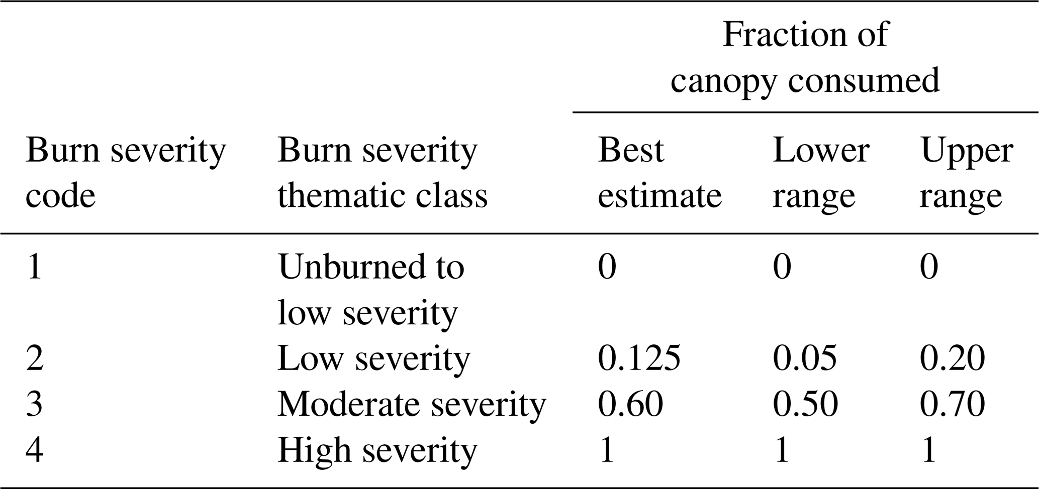
Best estimates and ranges of consumption (i.e., combustion completeness) for forest surface and understory fuels for the four moisture regimes used in the emission inventory are shown in Table 6. The best-estimate values are based on simulations using algorithms from the fire effects models CONSUME (Prichard et al., 2006) and FOFEM (Lutes, 2016a). The ranges, which were used to estimate uncertainty in the fuel consumption simulations, were assigned as 10 %–20 %. The best estimate and range for the fraction of forest canopy fuel consumed was based on each pixel's burn severity classification (Table 7), which was assigned as described in Sect. 2.3.3. Fuel consumption for shrub and herbaceous grid cells used the natural fuel equations from CONSUME (Prichard et al., 2006). The rangeland fuel consumption equations used do not include fuel moisture content and therefore were independent of the moisture regime.

Table 6 Best estimates and ranges of the combustion completeness by fuel component according to moisture regime and forest type group. Best estimates are based on cited references. Low and high ranges are assigned as approximately ±20 %.

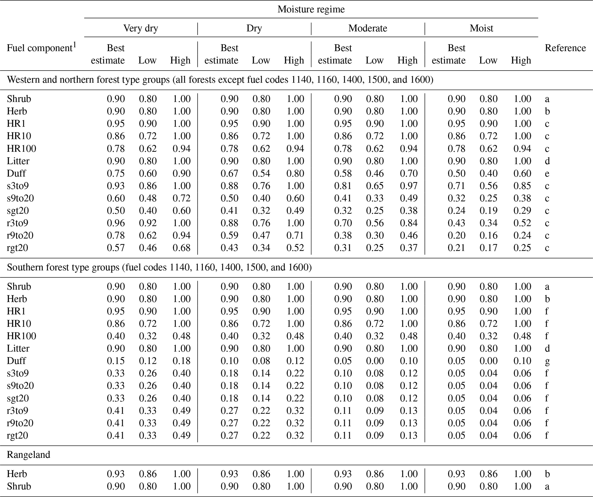
¹ See Table 3 for description.
References: (a) CONSUME natural fuel algorithm shrub stratum, adjusted to 0.90 (Prichard et al., 2006); (b) CONSUME natural fuel algorithm non-woody stratum, adjusted to 0.90 (Prichard et al., 2006); (c) CONSUME natural fuel algorithm – western woody equations (Prichard et al., 2006); (d) FOFEM default reduced to 0.90 (Lutes, 2016a); (e) Eq. (10) of Brown et al. (1985); (f) CONSUME natural fuel algorithm – southern woody equations (Prichard et al., 2006); (g) Hough (1978); (h) CONSUME natural fuel algorithm non-woody stratum (Prichard et al., 2006).

Table 7 Fraction of forest canopy consumed according to burn severity classification (after Miller and Yool, 2002).

2.7 Emission factors

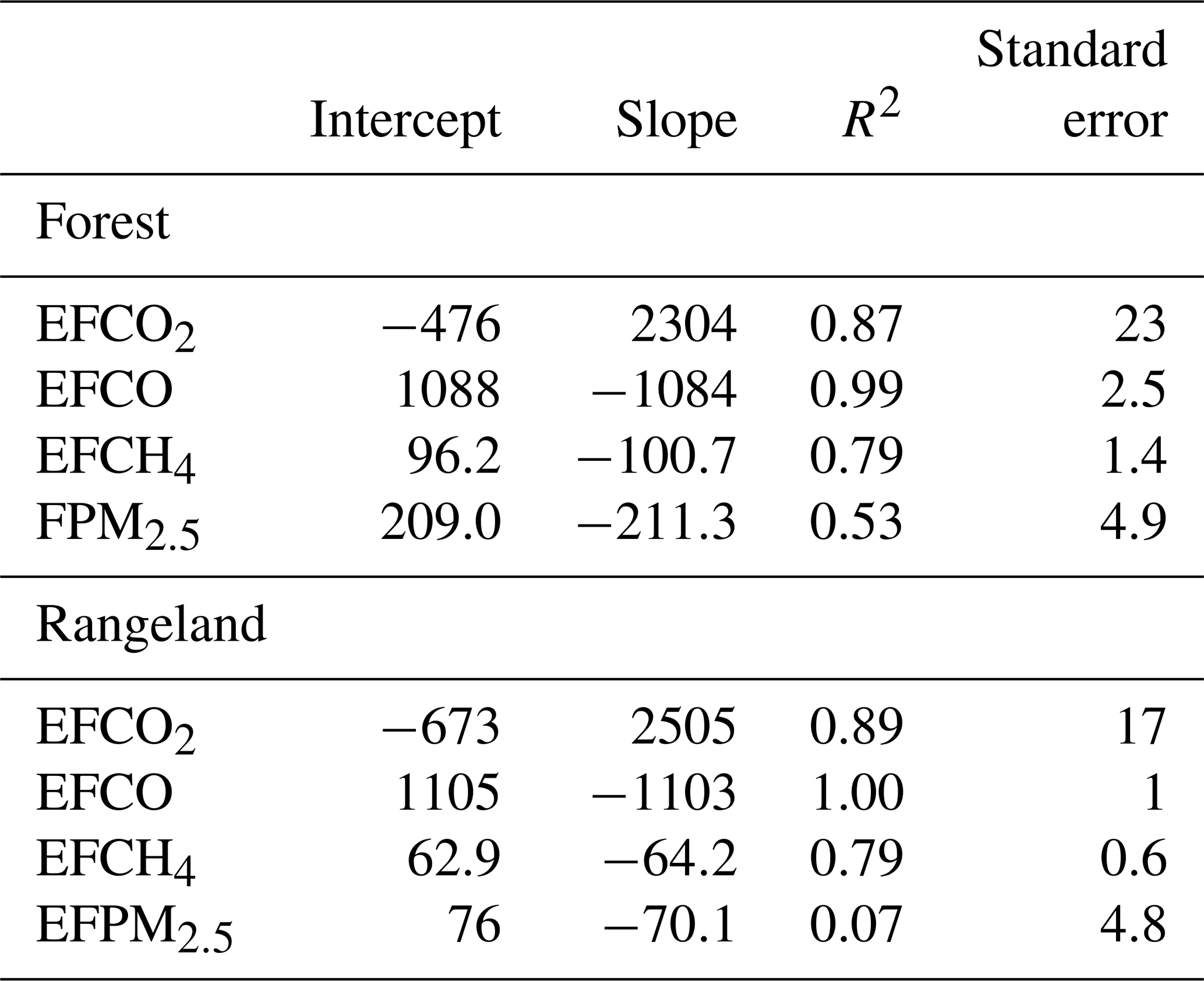
The composition and intensity of emissions produced by biomass burning varies with the relative mix of flaming and smoldering combustion. Modified combustion efficiency (MCE), the molar ratio of emitted CO₂ to the sum of emitted CO₂ and CO (MCE $=\mathrm{\Delta }{\mathrm{CO}}_{\mathrm{2}}/(\mathrm{\Delta }{\mathrm{CO}}_{\mathrm{2}}+\mathrm{\Delta }\mathrm{CO})$), is a widely used measure of the relative mix of flaming and smoldering combustion. Because the EFs of many species are correlated with MCE, it is a useful metric for extrapolating emission factors from one set of combustion conditions to another (Urbanski, 2014; Akagi et al., 2011). The MCE observed for wildland fires varies significantly across fire types; for example, average MCE values are around 0.94 and 0.93 for rangeland and southeastern forest fires, respectively, but ∼0.88 for wildfires in western forests (Urbanski, 2014). This difference in fire properties was accounted for in the emission inventory by using three sets of EFs (southern forests, western and northern forests, and rangeland). Data from several field studies (Table S4) were used to model EF as a linear function of MCE for forest and rangeland fires (Table 8). The linear functions were combined with best-estimate MCE values to derive the EF used in the inventory (Table 9). Since the focus of MFLEI is wildfires, the best-estimate MCE used for western and northern forests is based on western wildfires. Sufficient field measurement data of MCE and EF for southern wildfires could not be found in the literature. Therefore, the EFs used for southern forest fires are based on the large body of prescribed fire studies in the literature. The linear functions and their standard errors in Table 8 were combined with MCE values, sampled from a normal distribution to account for within-fuel-group uncertainty (Table 9), to provide an estimate of the uncertainty in the EF which was used in the emission modeling uncertainty analysis (Sect. 2.9).

Table 8 Statistics for the linear regression of EF as a function of MCE for field data from 78 forest fires and 20 rangeland fires (Table S4 and Figs. S1 and S2).

2.8 Emission estimates

The best estimates of fuel loading for the 14 fuel components (F_k,j, Table 3) were assigned to forest pixels using the mapped forest type group and associated fuel code (Sect. 2.2) and the FTG fuel classification system (Table 4). The fuel code, fuel moisture regime, and burn severity classification were used to designate combustion completeness by fuel component for each pixel (C_k,j) using the best estimates from Tables 6 and 7. Fuel loading for herbaceous and shrub pixels (F_k,j) was taken from the rangeland fuels map (Sect. 2.4.2). Herbs and shrubs were treated as single-component fuels with a combustion completeness that is independent of fuel moisture regime and burn severity classification. EF_k,i were selected from Table 9 based on the fuel type, and then the best-estimate emission intensities for CO₂, CO, CH₄, and PM_2.5 were calculated using Eq. (1).

Table 9 Best-estimate MCE and EF (g kg⁻¹) for generalized fire types from multiple field studies. The standard deviation for MCE is provided in parentheses. EFs are based on the linear fits in Table 8 at the fire type average MCE value. The MCE values are from Urbanski (2014).

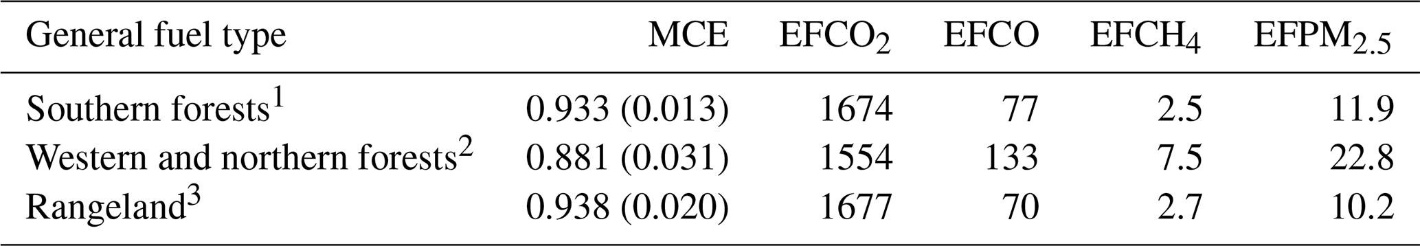
¹ Fuel codes 1140, 1160, 1400, 1500, and 1600. ² All forest fuel codes except 1140, 1160, 1400, 1500, and 1600. ³ Fuel codes 1 and 2.

2.9 Uncertainty estimates

A Monte Carlo style analysis following the general approach outlined in the IPCC Guidelines for National Greenhouse Gas Inventories (Eggleston et al., 2006) was used to estimate the uncertainty in emission intensities (kg m⁻²) at the pixel level. The method involved randomly selecting a sample of N input values (X_i, X_i+1, …, X_N) for the emission model (Eq. 1) and calculating emission intensities (E_i, E_i+1, …, E_N), where X_i is the array of input values needed for a single emission calculation: fuel loading by component (Table 3), combustion completeness (Tables 6 and 7), and EF (EFCO₂, EFCO, EFCH₄, EFPM_2.5), and E_i is the array of emission intensities for CO₂, CO, CH₄, and PM_2.5. The samples of input variables were generated based on each pixel's fuel code using the methods summarized in Table 10 and described in more detail below. The value of N was 500 for rangeland pixels. For forest pixels, N was taken as the greatest of 500 or N_plots, where N_plots is the number of plots in the FIA dataset for a given pixel's forest fuel code (Table 4). Next, quantiles (q=0.05, 0.10, 0.25, 0.50, 0.75, 0.90, 0.95) of the emissions (E_q,b) were calculated and saved. The process was repeated B times, yielding E_q,1, …, E_q,B, and mean values $\left(\sum _{\mathrm{1}}^B{E}_q/B\right)$ were calculated to provide uncertainty estimates of the emissions. Convergence of the distributions was achieved with B=2000.

Table 10 Sample generation methods employed in Monte Carlo style simulation of emission intensity uncertainty.

Forest surface fuels were generated by using fuel loading arrays sampled from the FIA plot data (included in the MFLEI dataset: file\Supplements\Fuel_Load_Plot_Data.csv; see Sect. 4); i.e., each element i used surface fuel components from a single FIA plot. This approach was chosen to preserve any correlations among surface fuel components. Uncertainty in the assigned moisture regime and burn severity classification, which are used to determine surface and canopy fuel consumption, respectively, were not considered in this analysis. Therefore, uncertainty analysis produced 464 sets of quantiles for forest pixels (29 forest fuel codes, four moisture regimes, and four burn severity classifications). Burned forest pixels were assigned sets of quantiles based on forest fuel code, moisture regime, and burn severity classification.

The variability in pixel-level shrub fuel loading was simulated using means and standard deviations based on the maps of the mean, minimum, and maximum loading (Sect. 2.4.2), with the standard deviation in loading estimated as half the range in maximum and minimum loading at each pixel. To reduce computational demands, shrub pixels were aggregated into bins of mean loading in 50 g m⁻² increments (50 to 5500 g m⁻²). For each 50 g m⁻² increment in mean loading, simulations were conducted using 25 increments of standard deviation, each corresponding to 10 percentage points of the mean loading value (10 % to 250 %), resulting in 2750 fuel loading elements (pairs of μ and σ). Similarly, pixel-level variability in herbaceous fuel loading was simulated based on pixel-specific mean and standard deviation from the maps of the mean and the coefficient of variation (C.V. = σ∕μ) of loading (Sect. 2.4.2). As with the shrub fuel loading, the herbaceous pixels were aggregated to reduce computational demands. Herbaceous pixels were grouped according to mean loading by 25 g m⁻² increments (25 to 500 g m⁻²). For each 25 g m⁻² increment in mean loading, simulations were conducted using 22 increments of standard deviation corresponding five percentage points of the mean loading value (from 5 % to 110 %), providing 440 fuel loading elements (pairs of μ and σ). Using the general approach described in the first paragraph of this section, a set of emission quantiles was produced for each of the 2750 shrub and 440 herbaceous fuel elements, with fuel loading simulated using a truncated normal distribution with the elements μ and σ, and the combustion completeness and EF using probability distributions described in Table 10. Since rangeland fuel consumption was estimated independent of moisture regime and burn severity classification, these variables were not considered in the uncertainty analysis. Each burned rangeland pixel was assigned a set of emission quantiles from the simulations based on its cover type (herb or shrub), fuel loading, and fuel load uncertainty.

The spatial and temporal resolutions required of fire emission inventory systems depend on the specific applications for which they are being used. For regulatory related air quality modeling, the EPA recommends a horizontal grid resolution of ≤12 km for O₃ and PM_2.5 NAAQS (USEPA, 2007). Therefore, the uncertainty estimation approach described above was applied aggregating burned pixels to a 10 km × 10 km grid. The resultant dataset at 1 day and 10 km spatial resolution provides a more relevant representation of the uncertainties of the emissions when used in typical air quality applications. The approach followed that outlined above, except that the emission intensities for each sample, E_i, were the sum of emission intensities for all pixels within each 10 km × 10 km grid cell on a given day. Only grid cell days with greater than four burned pixels were considered for this uncertainty analysis; this excluded 9 % of burned area over the 2003–2015 period.

Figure 10 Annual burned area, fuel consumed, and PM_2.5 emitted for 2003–2015.

3 Results

3.1 Annual, seasonal, and monthly

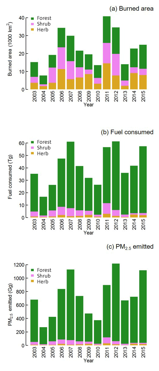
The MFLEI annual burned area, fuel consumed, and PM_2.5 emitted for 2003–2015 are shown in Fig. 10. The average area burned was 22 891 km² yr⁻¹; forests accounted for 44 % of burned area, with the balance split between herb (29 %) and shrub (27 %) cover types. The maximum annual burned area was 40 714 km² in 2011 which was >5 times the minimum of 7688 km² in 2004. The fuel consumed averaged 41.4 Tg yr⁻¹, with extremes of 16.6 Tg in 2004 and 61.2 Tg in 2012. The annual rank in fuel consumed differed from burned area due to the far greater fuel loading of forests (Sect. 2.4.3). While forests comprised only 44 % of burned area over the period, they accounted for 87 % of fuel consumed. Average PM_2.5 emissions were 733 Gg yr⁻¹ and, as with fuel consumed, 2004 and 2012 were the extreme years at 270 and 1216 Gg, respectively. There are slight differences in the ranking of annual fuel consumption and PM_2.5 emitted resulting from the different EFPM_2.5 used for southern and western/northern forests (Table 9). Maps of annual burned area, fuel consumed, and PM_2.5 emitted averaged over 2003–2015 are shown in Fig. 11. In the eastern two-thirds of the domain, fire activity and emissions are spread broadly across the southern tier, while being comparatively sparse in the north. In the west (western 11 states), fire activity has no latitudinal split, but there are large pockets where emissions are limited or absent. Many of the areas in the west without emissions are in desert regions of the southwest with sparse vegetation.

Figure 11 Annual burned area, fuel consumed, and PM_2.5 emitted averaged over 2003–2015.

Figure 12 Monthly distributions of burned area, fuel consumption, and PM_2.5 emitted over 2003–2015, broken down by cover type.

The monthly distributions of burned area, fuel consumption, and PM_2.5 emitted over 2003–2015, broken down by cover type, are plotted in Fig. 12. Burned area has a bimodal distribution with peaks in April and August. Summer (June, July, August) and spring (March, April, May) accounted for 49 % and 31 % of burned area, respectively. The ratio of herb and shrub to forest burned area was similar for summer (1.3) and spring (1.5) but differed considerably between the peak months of April (2.7) and August (1.0). August was the most significant month for emissions, accounting for 32 % PM_2.5 emitted, more than twice the share of the next highest month, which was July at 15 %. While April had the third highest burned area (15 % of total), it accounted for only 6.7 % of PM_2.5 emitted. The geographic distribution of emissions varies considerably by season, as may be seen in Fig. 13.

Figure 13 Seasonal PM_2.5 emitted average over 2003–2015.

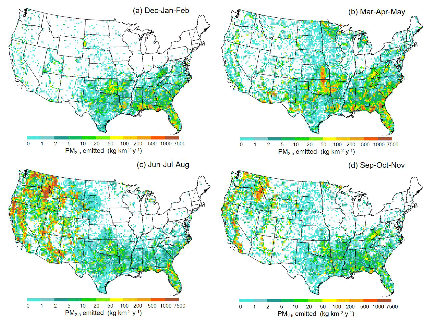
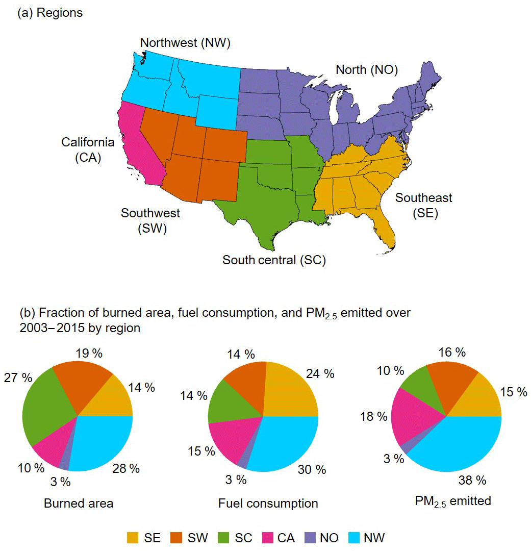
Figure 14 (a) Geographic regions. (b) Burned area, fuel consumption, and PM_2.5 emitted by region.

Understanding the spatiotemporal distribution of emissions is aided by aggregating the emissions according to six regions in Fig. 14. Roughly 8 % of fuel consumption and 6 % of PM_2.5 emissions occurred in the winter months (Fig. 12) and were largely limited to the southeast and south-central regions (Fig. 13). Winter PM_2.5 emissions comprised 25 % and 16 % of total PM_2.5 emissions in the southeast and south-central regions, respectively (Fig. 15). In the southeast, 74 % of winter emissions resulted from fire activity in Florida and along the Gulf Coast. The majority of southeast (52 %) and south-central (62 %) emissions occurred in the spring. Fires in the Flint Hills region of eastern Kansas and northeast Oklahoma accounted for 44 % of south-central spring emissions over the 13-year period. Summer was the most significant season for fuel consumption and emissions due to fire activity in the west (Fig. 13). The majority of CONUS-wide fuel consumption (51 %) and PM_2.5 emissions (59 %) occurred during the summer. On a regional basis, southwest emissions peaked during June (46 %) and during August in both the northwest (59 %) and California (40 %). Northwest emissions were concentrated in July–September (95 %), while California emissions were spread symmetrically across June–October (Fig. 15).

Figure 15 Monthly PM_2.5 emitted averaged over 2003–2015.

Figure 16 Fraction of regional 2003-2015 PM_2.5 emissions released on peak days.

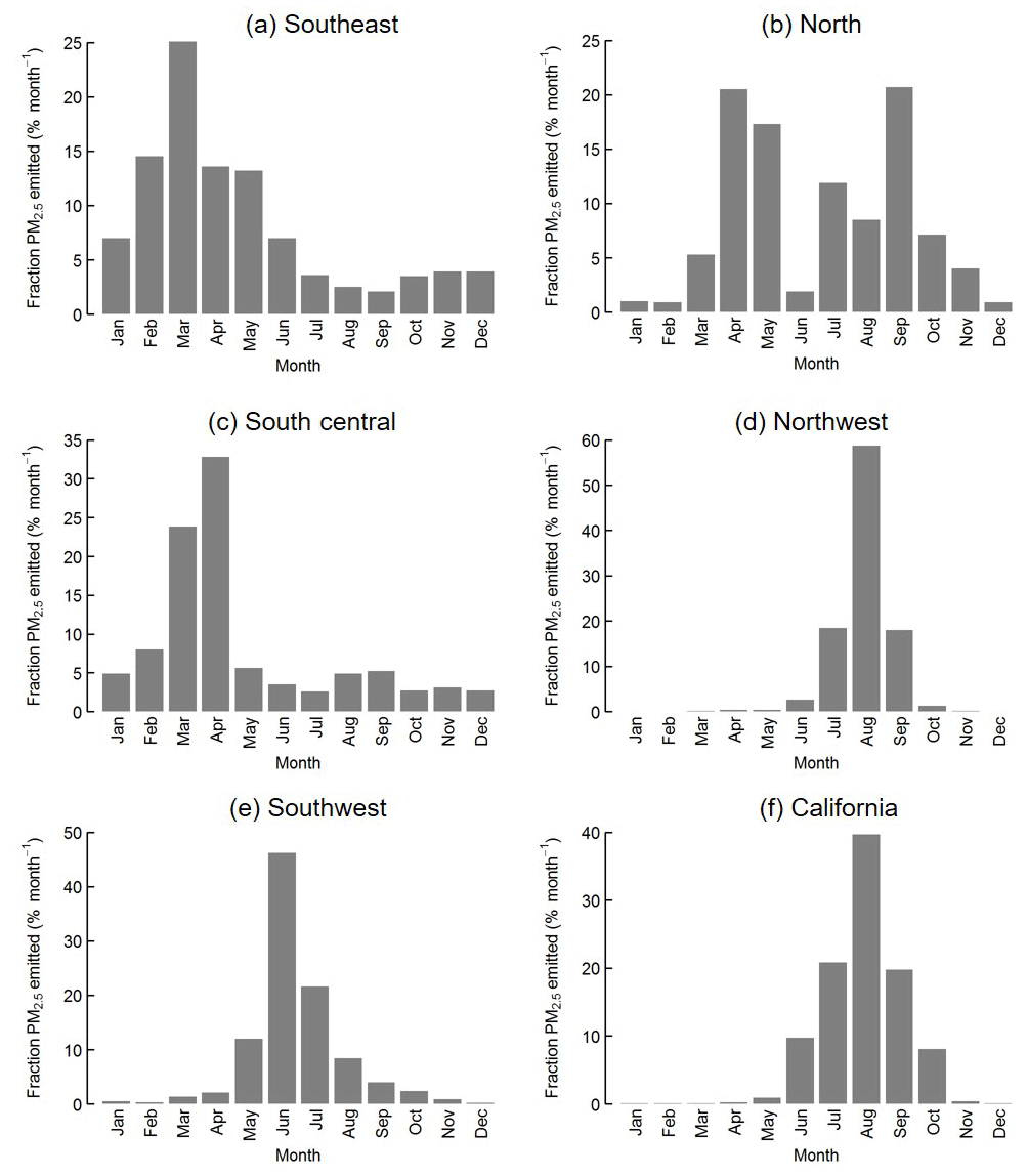
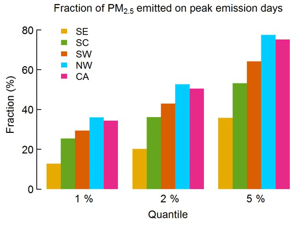
Figure 17 Cumulative distribution of daily PM_2.5 emissions aggregated on a 10 km × 10 km grid. The dashed line and dashed–dotted line mark 5 % and 10 % of grid cell days with emissions.

3.2 Daily

While regional-level summaries on a seasonal or monthly basis are useful for understanding the general spatiotemporal distribution of wildfire emissions, daily emissions are more relevant for appreciating the potential air quality impacts of fires. For instance, US NAAQS includes a 24 h standard for PM_2.5 and an 8 h standard for O₃ (the latter of which can be produced through photochemical processing of volatile organic compounds (VOCs) and NO_x present in smoke plumes (Jaffe and Wigder, 2012). Wildfires are highly episodic and even though they may persist for weeks, a significant share of a wildfire's emissions generally occur on a handful of days. For example, consider the typical large (>2000 ha) wildfire in the west: our inventory indicates more than half of its total PM_2.5 emissions occur on a single day. In the west, 1171 fires > 2000 ha in size accounted for ∼85 % of burned area and PM_2.5 emission from 2003 to 2015. To characterize wildfire temporal intensity, emissions of PM_2.5 were summed by region for each of the 4748 days of the inventory. Figure 16 plots the fraction of regional 2003–2015 PM_2.5 emissions released on peak emission days for the top first, second, and fifth quantiles of days. Since the north accounted for only 3 % of total wildfire emissions, it has been excluded from this analysis to simplify the discussion. Figure 16 shows that a small fraction of days (5 %) are responsible for the majority of wildfire PM_2.5 emissions in all regions except the southeast regions. In fact, the percent of PM_2.5 emissions during just the top 1 % of days was >33 % in California and the northwest, >25 % in the south-central and southwest, and ∼13 % in the southeast. The spatiotemporal concentration of emissions is further illustrated in Fig. 17, which plots the cumulative distribution of daily PM_2.5 emissions aggregated on a 10 km × 10 km grid. A total of 5 % of the grid cell days produced 69 % of total PM_2.5 emitted, and 10 % of grid cell days were responsible for 82 % of total PM_2.5 emitted. This analysis highlights the importance of quantifying wildfire emissions on a daily time step when assessing the potential impacts of wildfires on regional air pollution; assessments based on emissions aggregated seasonal, monthly, or even weekly time steps may significantly understate the likelihood of acute pollution episodes.

Figure 18 Annual PM_2.5 emitted in the west.

3.3 Comparison with non-fire emission sources

Next, we compare our wildfire PM_2.5 emissions with those from other sources as estimated in the EPA 2014 National Emission Inventory (NEI14; USEPA, 2014). We focus on the west (the 11 states of the northwest, southwest, and California regions; Fig. 14a) since this region accounts for 72 % of total wildfire PM_2.5 emissions (Fig. 14b), and the emissions are produced with a high temporal intensity (Figs. 15 and 16) and have resulted in severe air pollution episodes (Fann et al., 2018; Kochi et al., 2012; Rappold et al., 2014). Non-fire PM_2.5 emission estimates for the western states were extracted from the NEI14 Tier 3 summary state-level data (USEPA, 2018c). The NEI14 PM_2.5 emissions were limited to non-fire sources by excluding the Tier 3 source categories of “agricultural fires”, “forest wildfires”, and “prescribed burning”. The NEI14 provides annual emission estimates for 2014, which are plotted with the annual sum of MFLEI PM_2.5 emissions for the west for 2003–2015 in Fig. 18. The 2003–2015 annual average western wildfire PM_2.5 emitted is 525 Gg yr⁻¹ (range 126–1034 Gg yr⁻¹) compared with the non-fire source strength of 657 Gg yr⁻¹ in 2014. As discussed above, when inferring possible air quality impacts of wildfire emissions, 1 day is an appropriate timescale. Assuming the NEI14 emissions are a reasonable proxy for annual non-fire emissions across 2003–2015, and neglecting the seasonal variability of emissions, daily non-fire PM_2.5 emissions are 1.80 Gg d⁻¹. For all 4748 days of the MFLEI period, we calculated the wildfire-to-non-wildfire PM_2.5 emission ratio; the number of days the ratio exceeds certain thresholds is shown in Fig. 19. Across the west, wildfire emissions greatly exceed non-fire sources on active fire days. On ∼10 % of days, wildfire emissions are more than twice non-fire sources, and on 60 days, they were >10 times non-fire sources.

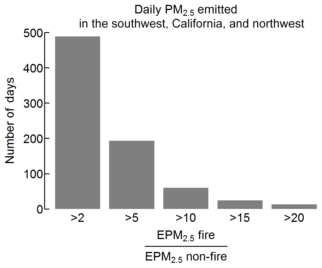
Figure 19 Number of days over 2003–2015 when the wildfire-to-non-wildfire PM_2.5 emission ratio in the west exceeds thresholds of 2, 5, 10, 15, and 20.

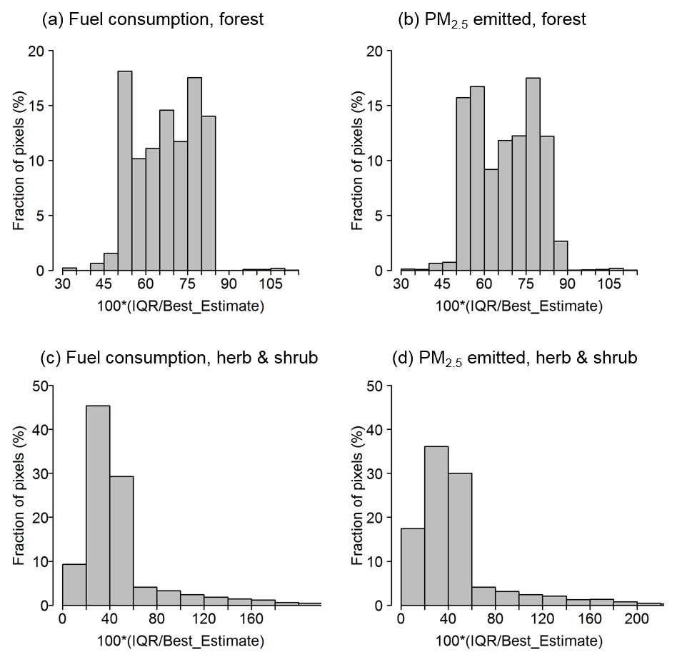
Figure 20 Distribution of relative interquartile range from pixel-level Monte Carlo style simulations.

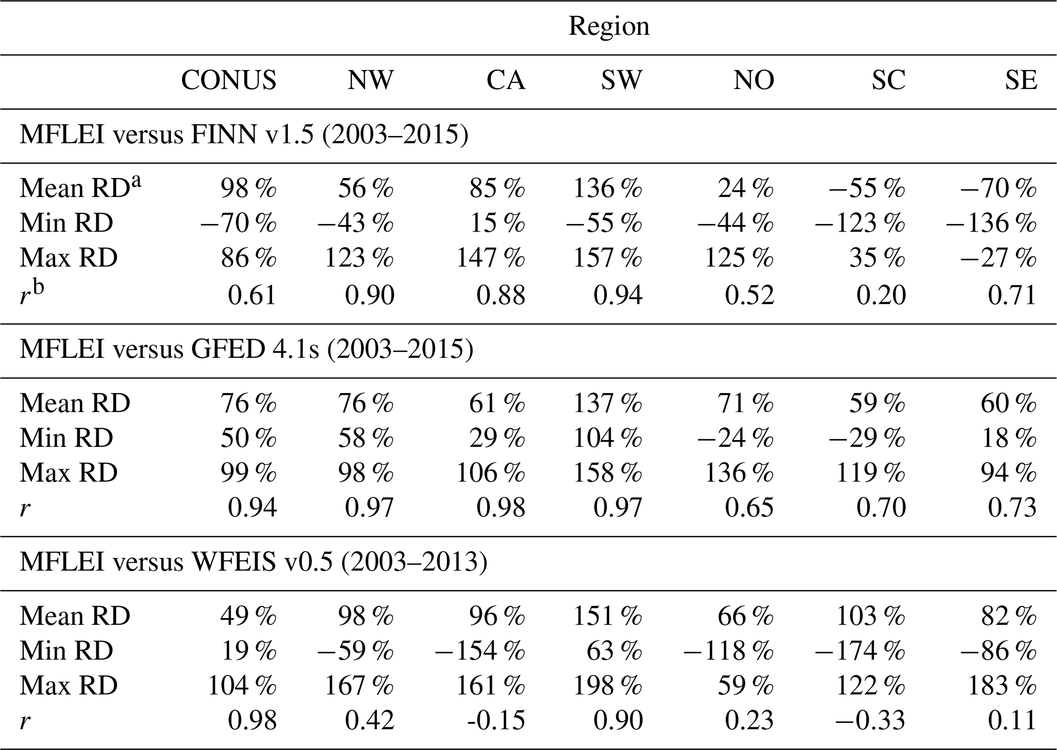
Table 11 Statistics for comparison of annual fuel consumption by region between MFLEI and FINN v1.5, GFED v4.1s, and WFEIS v0.5. Regions are as defined in Fig. 14a.

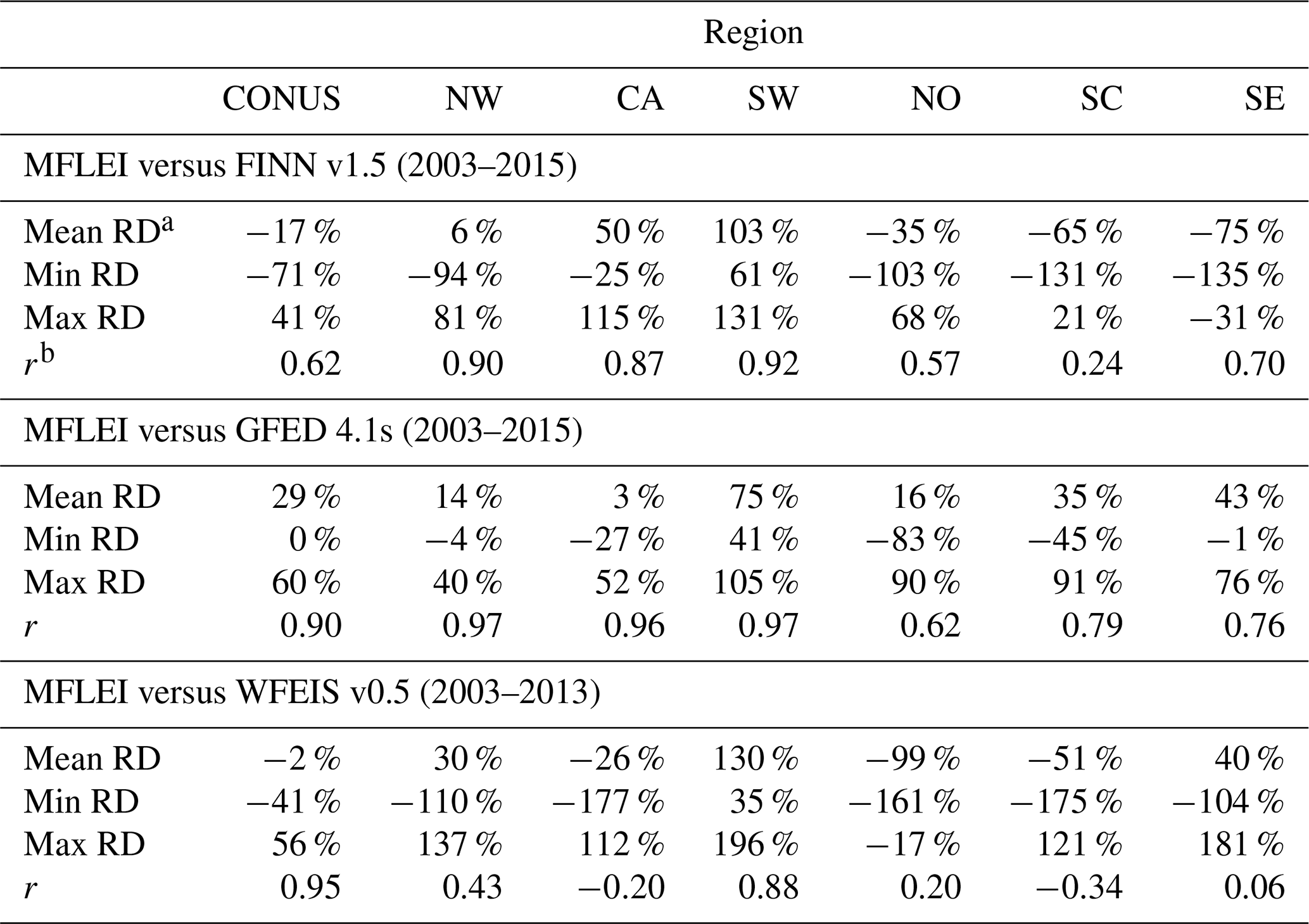
^a RD $=\mathrm{100}\times \frac{X(t{)}_{\text{MFLEI}}-Y(t{)}_i}{\mathrm{0.5}\times \left(X(t{)}_{\text{MFLEI}}+Y(t{)}_i\right)}$; X(t)_MFLEI= MFLEI fuel consumed in year =t; Y(t)_i=i fuel consumed in year =t, where i is FINN, GFED, or WFEIS. ^b r is the correlation coefficient.

3.4 Uncertainty

The MFLEI pixel-level best estimates of fuel consumption (FC) and emissions (ECO₂, ECO, ECH₄, EPM_2.5) were derived as described in Sect. 2.8, and the uncertainties in these estimates were characterized with quantiles (q=0.05, 0.10, 0.25, 0.50, 0.75, 0.90, 0.95) derived from Monte Carlo style simulations (Sect. 2.9). Here, we summarize the pixel-level uncertainty in terms of the relative interquartile range: RIQR $=(q_{\mathrm{75}}-q_{\mathrm{25}})/X$, where q₇₅ and q₂₅ are the 75 % and 25 % quantiles, and X is the best estimate of FC or EPM_2.5; the distributions are shown in Fig. 20. The mean RIQRs of both FC and EPM_2.5 are ∼67 % for forest cover type and ∼47 % for herb/shrub. At the pixel level, the uncertainty is driven by the variability in fuel loading. The difference in the uncertainty estimates between forest and herb/shrub cover types results primarily from the high variability in forest fuel loading (Fig. 4). The mean RIQRs are nearly 50 % higher for forest compared with herb/shrub; however, the latter does have a long positive tail with ∼11 % of pixels having RIQR > 90 %. These high-uncertainty non-forest pixels are shrub vegetation with low fuel consumption (<350 g m⁻²).

As discussed in Sect. 3.2, CONUS wildfire emissions are temporally and spatially concentrated. Considering this spatiotemporal concentration of emissions and the grid spacing typical of regional- and national-scale air quality modeling (4–12 km; USEPA, 2007; NOAA, 2018), we also estimated the uncertainty in daily MFLEI emissions aggregated on a 10 km × 10 km grid (Sect. 2.9). For purposes of air quality modeling and air regulatory activities, the uncertainty of these spatially aggregated emissions provides a more relevant metric than the pixel-level uncertainty presented above. Uncertainties in the daily aggregated FC and PM_2.5 emissions are shown in Fig. 21a–b, expressed in terms of the RIQR (calculated using the quantiles and best estimates for the spatially aggregated data). Compared with the pixel-level data, the RIQR is reduced for the aggregated emissions and a difference emerges between FC and EPM_2.5; the mean RIQR is 17 % for FC and 26 % for EPM_2.5. For the aggregated data, we also show, in Fig. 21c–d, the distribution of relative interdecile range, RIDR $=(q_{\mathrm{90}}-q_{\mathrm{10}})/X$, where q₁₀ and q₉₀ are the 10 % and 90 % quantiles (Monte Carlo style simulations; Sect. 2.9), and X is the best estimate for FC or EPM_2.5. The mean RIDR is 32 % for FC and 50 % for EPM_2.5.

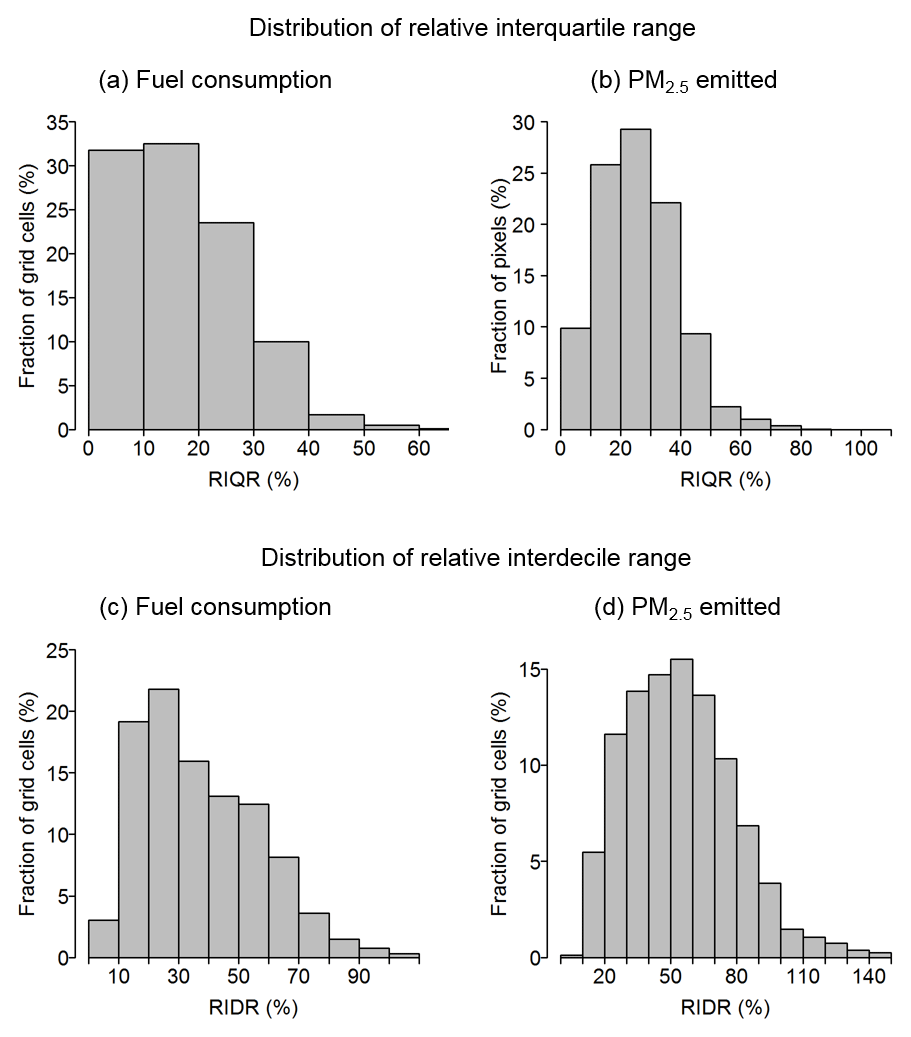
Figure 21 Distribution of relative interquartile range (a, b) and relative interdecile range (c, d) from 10 km × 10 km gridded Monte Carlo style simulations.

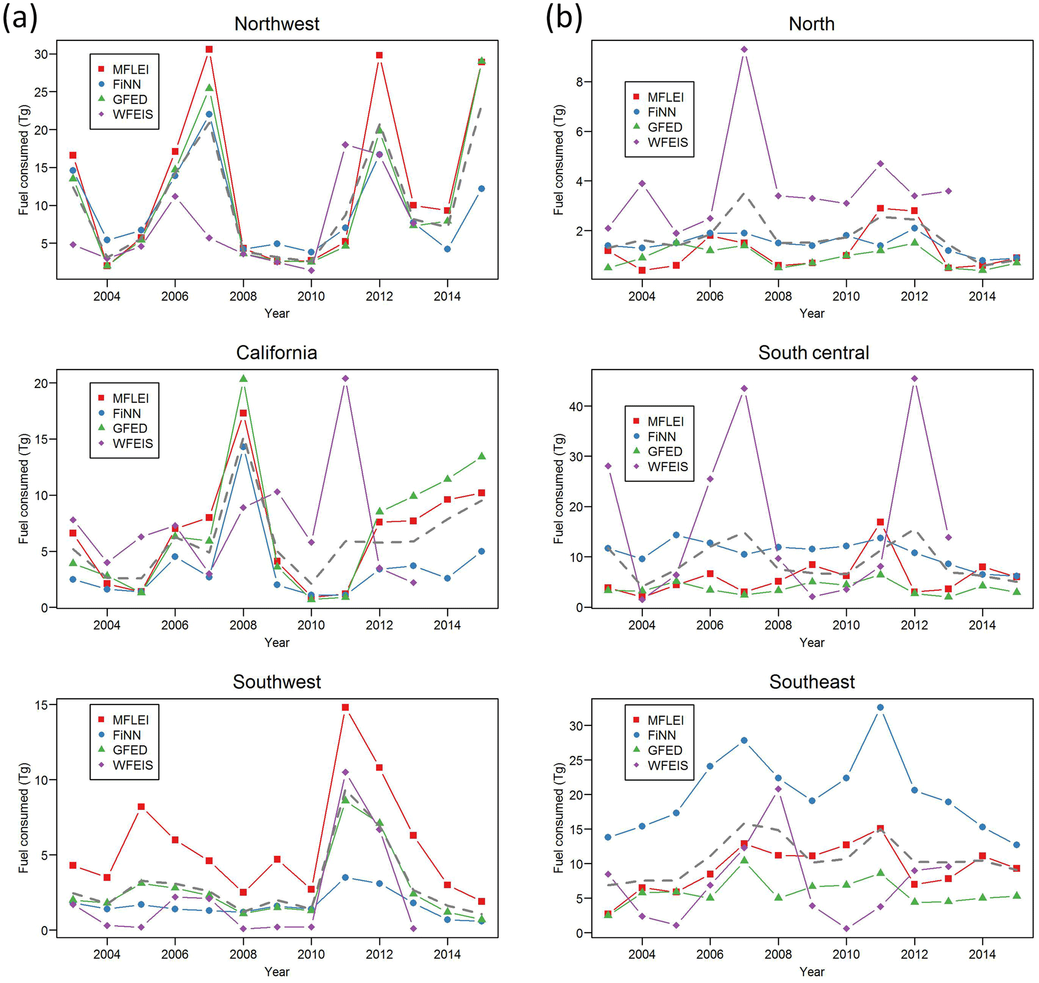
Figure 22 Annual fuel consumption from MFLEI, FINN v1.5, GFED v4.1s, and WFEIS v0.5 for (a) northwest, California, and southwest regions and (b) north, south-central, and southeast regions.

3.5 Prescribed fires

While the focus of MFLEI is wildfires, it does include an unquantified contribution from prescribed fires (fires intentionally ignited to achieve land management objectives). The MTBS product does contain large (>404 ha the west and >202 ha elsewhere) prescribed fires; over 2003–2015, ∼13 % of the MTBS burned area was due to fires classified as prescribed or unknown. Additionally, the MODIS burned area product (Giglio et al., 2015) used to supplement MTBS does not distinguish between wildfires and prescribed fires and likely includes some prescribed fire burned area. Information on prescribed fires by federal and state agencies indicates an average fire size of ∼60 ha (NIFC, 2018). Considering the large fire focus of MTBS and the fact that prescribed fires are often low-intensity understory burns, which are difficult to detect by satellite (Hawbaker et al., 2008), we believe prescribed fires account for a small share of total MFLEI emissions. Unfortunately, there is no nationwide database that inventories prescribed fire on federal, state, and private lands. The 2015 National Prescribed Fire Use Survey Report (Melvin, 2016), based on a 2014 comprehensive survey conducted by state forestry agencies, summarizes prescribed fire activity at national and regional levels. Melvin reported CONUS prescribed fire burned area as 35 222 km² in 2014. For the same year, the MTBS prescribed fire burned area was 11 954 km² (prior to reduction for unburned to low burn severity patches as described Sect. 2.3.3), suggesting MFLEI may be missing up to two-thirds of CONUS prescribed fire burned area. The regional summary in Melvin reports prescribed fire burned area of 25 049 km² in their southeast region (the southeast and south-central regions used in our study, excluding Kansas and Missouri). The 2014 MTBS data report only 4651 km² of prescribed fire burned area for the same region, indicating most of MFLEI underrepresentation in prescribed fire emissions occurs in these southern states.

Table 12 Statistics for comparison of annual PM_2.5 emitted consumption by region between MFLEI and FINN v1.5, GFED v4.1s, and WFEIS v0.5. Regions are as defined in Fig. 14a.

^a RD $=\mathrm{100}\times \frac{X(t{)}_{\text{MFLEI}}-Y(t{)}_i}{\mathrm{0.5}\times \left(X(t{)}_{\text{MFLEI}}+Y(t{)}_i\right)}$; X(t)_MFLEI= MFLEI PM_2.5 emitted in year =t; Y(t)_i=i PM_2.5 emitted in year =t, where i is FINN, GFED, or WFEIS. ^b r is the correlation coefficient.

3.6 Comparison with other emission inventories

Next, we compare the estimated fuel consumption and PM_2.5 emissions of MFLEI with three fire emission inventories: GFED v4.1s (GFED, 2018), FINN v1.5 (NCAR, 2018), and WFEIS v0.5 (MTRI, 2018). In this comparison, we have excluded fuel consumption and PM_2.5 emissions associated with agricultural burning from all three inventories. Regional annual fuel consumption from the four inventories is plotted in Fig. 22. Statistics comparing MFLEI regional annual fuel consumption versus the other inventories are given in Table 11. There is significant variability in the agreement between MFLEI and the other inventories. Across the west (NW, CA, SW), MFLEI annual fuel consumption is well correlated with both FINN and GFED (Table 11). MFLEI fuel consumption exceeds the mean of FINN, GFED, and WFEIS in nearly all years and is generally the highest in northwest and southwest regions (Fig. 22a). In the east regions (SC, SE, NO), MFLEI fuel consumption fluctuates about the FINN/GFED/WFEIS mean value (Fig. 22b). In terms of variability and mean absolute relative difference, MFLEI agrees best with GFED.

Regional annual PM_2.5 emissions are shown in Fig. 23 and statistics comparing MFLEI PM_2.5 emissions versus the other inventories are given in Table 12. As with fuel consumption, across the west (NW, CA, SW), MFLEI annual PM_2.5 emissions are well correlated with both FINN and GFED, while correlation with WFEIS is weak in most regions (Table 12). In the west, MFLEI annual PM_2.5 emissions are highest among the inventories in most years (Fig. 23a). The greater PM_2.5 emissions of MFLEI in the west are partly attributable to the use of a larger EFPM_2.5 for western forests (22.8 g kg⁻¹, Table 9) compared with FINN (12.9 g kg⁻¹), GFED (12.6 g kg⁻¹), and WFEIS (11.9 g kg⁻¹). Because WFEIS uses combustion-phase-dependent EFs applied in a non-transparent manner, we have taken EFPM_2.5 as the ratio of the sum of EPM_2.5 to the sum of fuel consumed for all western forests. MFLEI uses EFPM_2.5 from the synthesis of Urbanski (2014) that accounts for the lower MCE measured for wildfires in western conifer forests (Urbanski, 2013). FINN and GFED use EFPM_2.5 from Akagi et al. (2011), with updates from May et al. (2014), which are based on emission measurements of prescribed fires, most of which occurred in the southeast US. WFEIS employs EFPM_2.5 measured for prescribed burns of logging slash. The higher EFPM_2.5 used by MFLEI for wildfires in western forests is consistent with recent emission measurements of Liu et al. (2017). In a study of western US wildfires, Liu et al. (2017) reported an average EFPM₁ of 26.0 g kg⁻¹ (PM₁ is particulate matter with an aerodynamic diameter < 1 µm), more than 2 times the EF for prescribed fires.

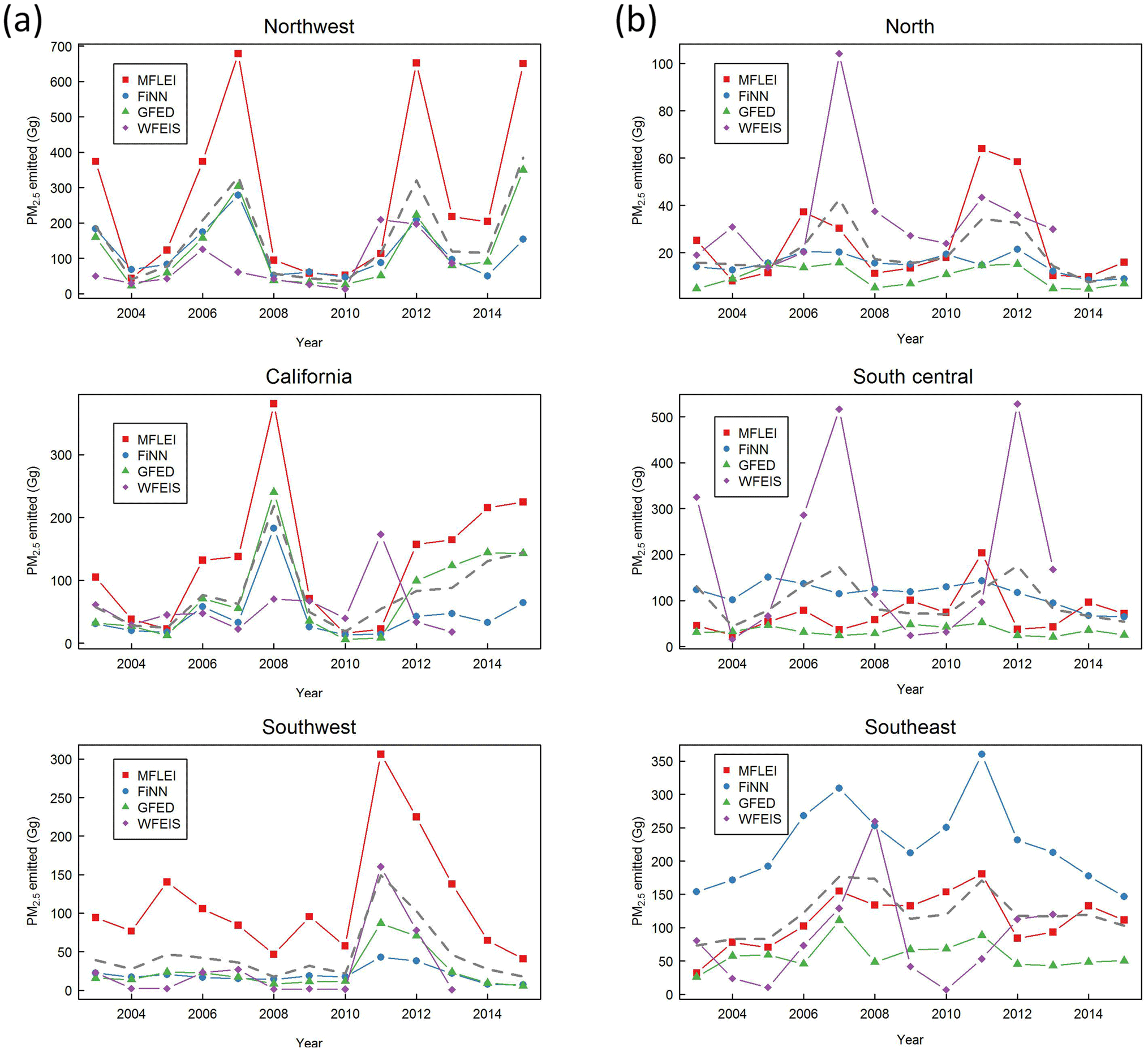
Figure 23 Annual PM_2.5 emitted from MFLEI, FINN v1.5, GFED v4.1s, and WFEIS v0.5 for (a) northwest, California, and southwest regions and (b) north, south-central, and southeast regions.

4 Data availability

MFLEI is archived and publicly available at the USDA Forest Service Research Data Archive with the DOI number https://doi.org/10.2737/RDS-2017-0039 (Urbanski et al., 2017).

5 Conclusions

We have presented the Missoula Fire Lab Wildfire Emission Inventory (MFLEI), a retrospective wildfire emission inventory for CONUS. MFLEI was developed from multiple datasets of fire activity and burned area, a newly developed wildland fuels map and an updated emission factor database. Daily burned area was constructed using a combination of Landsat-based burn severity data (MTBS), MODIS burned area and active fire detection products, VIIRS active fire detections, incident fire perimeters, and a spatial wildfire occurrence database. Forest fuel loading was based on a large set (> 27 000 sites) of forest inventory surface fuel measurements. Herbaceous fuel loading was estimated using site-specific parameters from a soil survey database with NDVI from MODIS. Shrub fuel loading was quantified by applying numerous allometric equations linking stand structure and composition to biomass and fuels, with the structure and composition data derived from geospatial data layers of the LANDFIRE project. MFLEI provides estimates of daily wildfire burned area, fuel consumption, and pollutant emissions at a 250 m × 250 m resolution for 2003–2015. The inventory includes a spatially aggregated emission product (10 km × 10 km, 1 day) with uncertainty estimates to provide a more relevant representation of emission uncertainties for use in air quality modeling. MFLEI will be updated with recent years as the MTBS data become available. The focus of MFLEI is wildfires and does not include most prescribed fire activity. In the southeast, where prescribed fire burned area is estimated to greatly exceed that of wildfires on average, the prescribed fire emissions not included in MFLEI are likely to be substantial.

MFLEI CONUS average wildfire fuel consumption and PM_2.5 emissions were estimated to be 41.4 Tg yr⁻¹ and 733 Gg yr⁻¹, respectively, over 2003–2015. Annual CONUS PM_2.5 emissions showed significant variability with a coefficient of variation of 0.41 and a maximum-to-minimum ratio of 4.5. Summer was the most active season; over half (59 %) of total PM_2.5 emissions occurred in the summer (June–August), with August alone accounting for 32 % of the total. Emissions were highly concentrated both temporally and spatially. Just 5 % of days accounted for 57 % of total PM_2.5 emitted over 2003–2015. At the spatial scale of the 10 km × 10 km grid, 69 % of total PM_2.5 originated from 5 % of grid cell days with fire activity. Fires in the west (western 11 states) accounted for 56 % of burned area, 60 % of fuel consumption, and 72 % of PM_2.5 emitted over 2003–2015. The southeast and south-central regions were largely responsible for the balance of burned area and emissions. The northern tier states across central and eastern CONUS produced <3 % of total PM_2.5 emissions. In the west, wildfire PM_2.5 emissions dwarfed those from non-fire sources during active fire periods. Comparison of MFLEI PM_2.5 emissions with the EPA 2014 National Emission Inventory indicated that, in the west, wildfires exceeded all non-fire primary sources of PM_2.5 by a factor of >5 on nearly 200 days over 2003–2015. Quantified with the relative interdecile range, the uncertainties in daily fuel consumption and PM_2.5 emissions, at the spatial scale of 10 km × 10 km, were estimated to be 32 % and 50 %, respectively. A regional comparison of MFLEI with three fire emission inventories, FINN v1.5, GFED v4.1s, and WFEIS v0.5, showed MFLEI predicted significantly greater PM_2.5 emissions across the west, in part due to the use of a larger EFPM_2.5 for wildfires in forests.

Appendix A

Table A1 Average small fire duration based on the fire discovery and containment dates from the years 2003–2015 of the Fire Occurrence Database (Short, 2017).

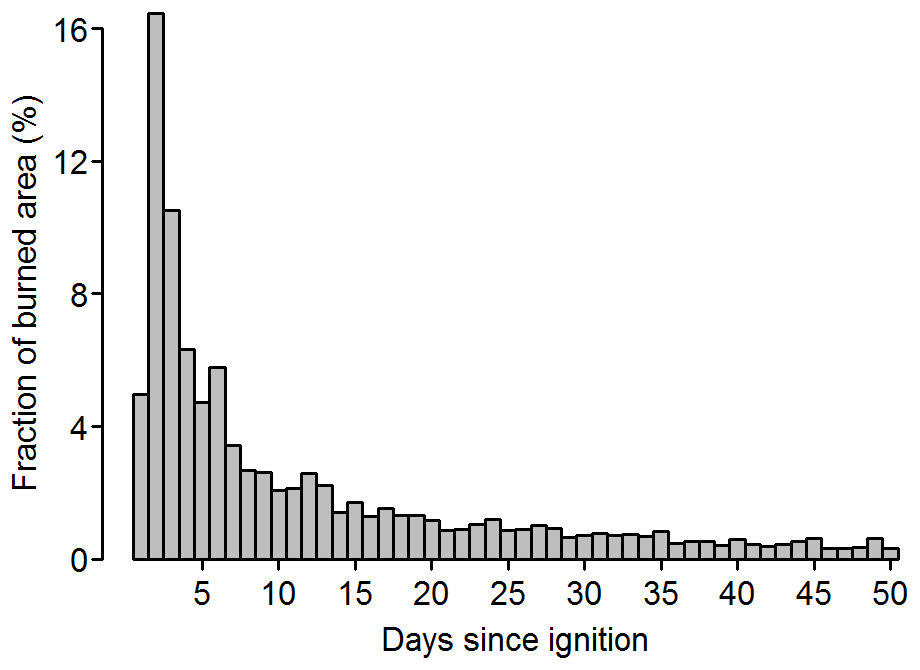
Figure A1 The burn-day distribution for the 12 500–25 000 ha size class. Distributions for all six size classes are provided in the Supplement dataset (file\Supplements\BurnDayDist.csv).

Appendix B

Table B1 ACF best estimates (see Sect. 2.4.1) and optimized parameters for Weibull PDF fits. Parameters predict ACF in units of t acre⁻¹.

¹ N is the number of FIA plots used in deriving best-estimate ACF and Weibull PDF fits. ² Values for fuel code 1990 are set to those for fuel code 1980 due to lack of data.

Appendix C

Table C1 Thematic classes representing shrub heights in the LANDFIRE EVH product and the associated height values represented in the RVS fuel modeling system.

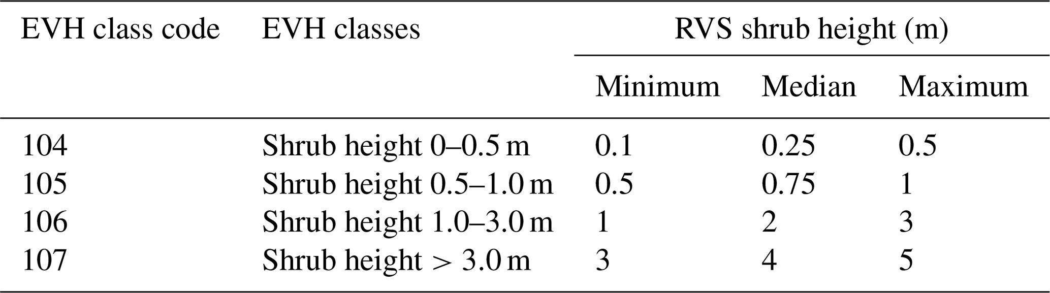
This appendix demonstrates the four-step process used to estimate shrub fuel loading. Three LF existing vegetation products are used: EVT, EVC, and EVH. The height estimates at each pixel in the EVH product are thematic classes representing a range of potential heights (Table C1) which enables three values of shrub fuels to be estimated at each pixel (average, maximum, and minimum). Likewise, the EVC product is thematic classes providing a 10-percentage-point range in potential vegetation cover (Table C2). However, the shrub fuel loading calculation simply uses the median value vegetation cover range. To illustrate, consider a pixel with an EVT of class of big sagebrush shrubland, an EVH class of 105, and an EVC class of 112; the fuel loading calculation proceeds as described below.

First, the crown volume is derived from the three EVH estimates (0.5, 0.75, and 1.0 m) as the product of these EVH values and the projected crown area on a horizontal surface (PCH), the latter of which is estimated using Eq. (C1) (Frandsen, 1983):

$$\begin{array}{}\text{(A1)}& {\log }_{\mathrm{10}}\left(\mathrm{PCH}\right)=-\mathrm{0.8471}+\mathrm{2.2953}{\log }_{\mathrm{10}}\left(\text{HT}\right),\end{array}$$

where PCH is the projected horizontal crown area in cm² and HT is the estimated shrub height in centimeters (from the EVH product). Per stem aboveground biomass estimates are then derived from the crown volume estimates using an allometric equation for sagebrush shrubs from the RVS allometry library:

$$\begin{array}{}\text{(A2)}& \text{PSB}=\mathrm{201.4062}+\mathrm{1.162}\times \text{VOL},\end{array}$$

where PSB is per stem biomass (g stem⁻¹) and VOL is crown volume (dm³). Next, the pixel stem density (SD; stem ha⁻¹) is estimated to expand PSB to a per area basis:

$$\begin{array}{}\text{(A3)}& \text{SD}=\left({\displaystyle \frac{\mathrm{1.0}\times {\mathrm{10}}^{\mathrm{8}}}{\mathrm{PCH}}}\right)\times \text{CC},\end{array}$$

where SD is stem density, CC is the fractional canopy cover from EVC (Table C2), and the value 1.0×10⁸ converts cm² to a per hectare basis. The total shrub biomass (TSB; kg ha⁻¹) is the product of PSB and SD. Figure C1 shows the TSB estimates for the pixel used in this example. This process was conducted at each pixel with a shrub EVT using the range of heights from EVH to provide lower, upper, and middle estimates of fuel loading. The allometric equation used to estimate PSB depends on the pixel EVT and is selected from 31 equations available in the RVS allometry library.

Table C2 Thematic classes representing shrub canopy in the LANDFIRE EVC product and the associated canopy cover used in the RVS fuel modeling system.

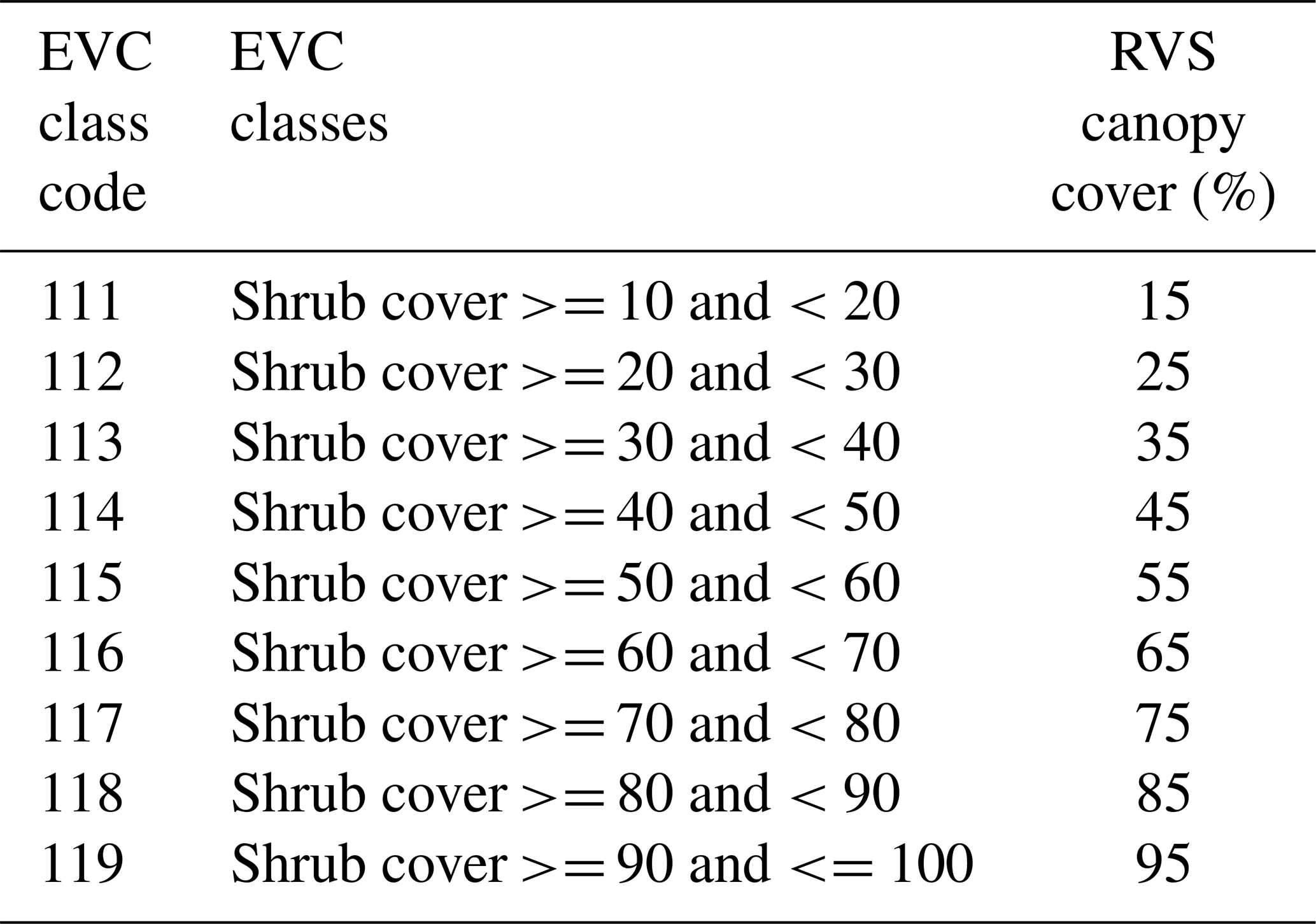
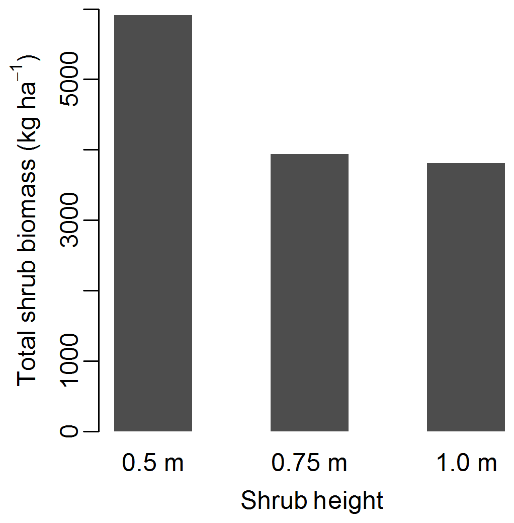
Figure C1 Total shrub biomass estimates for a pixel with EVT class of big sagebrush shrubland, EVH class of 105, and EVC class of 112 (see text).