A high-resolution air temperature data set for the Chinese Tian Shan in 1979–2016

The Chinese Tian Shan (also known as the Chinese Tianshan Mountains, CTM) have a complex ecological environmental system. They not only have a large number of desert oases but also support many glaciers. The arid climate and the shortage of water resources are the important factors restricting the area's socioeconomic development. This study presents a unique high-resolution (1 km, 6-hourly) air temperature data set for the Chinese Tian Shan (41.1814–45.9945^∘ N, 77.3484–96.9989^∘ E) from 1979 to 2016 based on a robust elevation correction framework. The data set was validated by 24 meteorological stations at a daily scale. Compared to original ERA-Interim temperature, the Nash–Sutcliffe efficiency coefficient increased from 0.90 to 0.94 for all test sites. Approximately 24 % of the root-mean-square error was reduced from 3.75 to 2.85 ^∘C. A skill score based on the probability density function, which was used to validate the reliability of the new data set for capturing the distributions, improved from 0.86 to 0.91 for all test sites. The data set was able to capture the warming trends compared to observations at annual and seasonal scales, except for winter. We concluded that the new high-resolution data set is generally reliable for climate change investigation over the Chinese Tian Shan. However, the new data set is expected to be further validated based on more observations. This data set will be helpful for potential users to improve local climate monitoring, modeling, and environmental studies in the Chinese Tian Shan. The data set presented in this article is published in the Network Common Data Form (NetCDF) at https://doi.org/10.1594/PANGAEA.887700. The data set includes 288 nc files and one user guidance txt file.

1 Introduction

Near-surface air temperature is the primary indicator of climate change and significantly impacts local as well as global water, energy, and matter cycles (e.g., Bolstad et al., 1998; Gao et al., 2012, 2014a; Prince et al., 1998). Air temperature is a necessary input variable for most hydrological and environmental models because it controls a large number of environmental processes. Long-term and high-resolution temperature data including historic, current, and future series are a prerequisite for accurate climate change assessment particularly on a regional scale (Gao et al., 2012; Minder et al., 2010; Maurer et al., 2002; Mooney et al., 2011; Pepin and Seidel, 2005). However, as the most common sources for air temperature time series, observational networks suffer from low station density in complex terrains, in particular high mountainous areas (Gao et al., 2014a). The installation and maintenance of stations in these regions are the main challenges (Kunkel, 1989; Rolland, 2003). To obtain spatially continuous temperature data, interpolation technologies such as natural neighborhood, inverse distance weighting, and a series of kriging methods are usually applied. However, these methods rely on the density of surface stations. The reliability of interpolated results decreases with increasing distance from the selected stations, particularly when using the inverse distance weighting method. Thus, interpolation approaches may induce large errors for a large region with a low density of stations (e.g., Vogt et al., 1997).

In contrast to the low availability of observations, reanalysis products provide long-term and spatially consistent data sets and have been increasingly applied for climate change assessment during the past 2 decades (e.g., Gao et al., 2014a; Mooney et al., 2011). Reanalysis is designed to estimate the state of real atmosphere and land surface characteristics by assimilating a large number of observations (Decker et al., 2012; Simmons et al., 2010). However, reanalysis contains uncertainties, such as observational changes and model misrepresentation (Simmons et al., 2010). With the development of a reanalysis assimilation system, the spatial resolution has been enhanced to 0.125^∘, for example ERA-Interim. However, local processes such as temperature inversions in deep valleys as well as snowpack accumulation and melting are still not explicitly considered. Furthermore, because of the heterogeneity over the land surface, many hydrological and climatic impact models use applications of high resolution, which tend to run on a scale of 0.1–1 km (Bernhardt and Schulz, 2010; Gao et al., 2012; Maraun et al., 2010). To this end, downscaling and correcting reanalysis data are necessary (Gao et al., 2012, 2014b, 2016).

Previous studies have shown that the elevation difference between the reanalysis grid point and the corresponding meteorological station leads to a large systematic bias (Gao et al., 2012, 2014a, 2016). Thus, an elevation correction scheme based on a lapse rate, which explains the empirical relationship between air temperature and altitude, can significantly reduce this bias. A constant lapse rate within a range of −6.0 to −6.5 ^∘C km⁻¹ (e.g., Dodson and Marks, 1997; Lundquist and Cayan, 2007; Marshall et al., 2007; Maurer et al., 2002) is commonly used. Monthly temperature gradients within the atmosphere are also widely applied in different regions (Kunkel, 1989; Liston and Elder, 2006). However, previous studies have shown that a fixed lapse rate may be problematic because the values of the lapse rate can significantly vary within short time periods of less than 1 month (Lundquist and Cayan, 2007; Minder et al., 2010; Rolland, 2003). To address this issue, using a lapse rate calculated from meteorological stations shows the best performance in many regions (e.g., Gao et al., 2012, 2017). However, the observed lapse rate completely relies on the density of sites, and it is not applicable for regions without observations, such as the high mountains.

Gao et al. (2012) introduced one other strategy that obtains temporal variability of lapse rates by calculating from temperatures and geopotential heights at different pressure levels of the ERA-Interim. For example, Γ_{500_700} represents the temperature lapse rate between the 500 and 700 hPa pressure levels. It is completely derived from ERA-Interim on internal pressure levels. It is therefore independent of local station observations. This method has been successfully applied in cases in the European Alps and on the Tibetan Plateau (Gao et al., 2012, 2017). Furthermore, this approach has the potential to be used to correct ERA-Interim temperature data for any other high mountainous areas. Following this approach, for the first time, $\mathrm{0.25}{}^{\circ }\times \mathrm{0.25}{}^{\circ }$, 6-hourly ERA-Interim 2 m temperature data from 1979 to 2016 were downscaled and corrected to 1 km, 6-hourly temperature data for the Chinese Tian Shan (also known as the Chinese Tianshan Mountains, CTM). The temperature data set presented here is extraordinarily unique because it covers such a large area of complex terrain with long-term continuous data both in space and time. The validation with observations from meteorological stations shows that this data set is generally reliable and suitable for climate change impact assessment as well as for hydrological and environmental modeling.

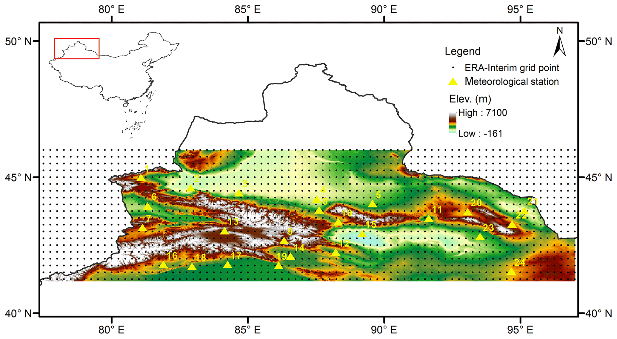
Figure 1 Location of the 24 meteorological stations (triangles) and ERA-Interim $\mathrm{0.25}{}^{\circ }\times \mathrm{0.25}{}^{\circ }$ grid points (dots). The elevation ranges from −161 m to 7100 m a.s.l., with a DEM resolution of 1 km.

Specific information regarding the CTM is described in Sect. 2. Used data including ERA-Interim and observations, elevation correction methods, and evaluation criteria are presented in Sect. 3. Section 4 provides the validation results, and the data accessibility is presented in Sect. 5. The discussion and conclusions are presented in Sect. 6.

2 Study area

The Tian Shan are among the seven major (and the largest) independent latitudinal mountain systems of the world. They span four countries including China, Kazakhstan, Kyrgyzstan, and Uzbekistan in the east–west direction. They stretch approximately 2500 km in length with an average width of 250–350 km (Chen et al., 2014; Hu, 2004; Wang et al., 2011). The eastern Tian Shan are termed the Chinese Tian Shan and extend over 1700 km into Xinjiang province, China (Fig. 1). They occupy approximately one-third of the entire area of Xinjiang province (∼ 570 000 km²). The CTM consist of three parallel mountain ranges (Hu, 2004; Wang et al., 2011). The north branch of the mountains mainly includes Ala Mount, Keguqin, Borokoonu, and Bogda mountains. The central branch includes Arakar, Nalati, Erwingen, and Hora mountains. The south branch mainly includes Kochsal, Khark, Lerke, and Karake mountains (Hu, 2004). The elevation decreases from west to east, with an average elevation of approximately 4000 m. The CTM also serve as a boundary between the northern and southern hillsides, as represented by the Junggar Basin and the Tarim Basin, respectively. Mt. Tomur is the highest peak of the Tian Shan at an elevation of 7443.8 m (Hu, 2004).

The Tian Shan have a special arid climatic regime because they are the furthest distance from the sea compared to that of other major mountain systems over the world. Many rivers such as the Syr, Chu, and Ili rivers originate in the Tian Shan (Chen et al., 2014, 2017; Hu, 2004). The CTM not only have a large number of desert oases in the basins, but also support a large number of glaciers. Statistically, there are 9035 glaciers in the CTM, with an area of 9225 km² and a volume of 1011 km³ (Shi, 2008; Shi et al., 2010). However, most of the glaciers in the CTM are in a state of rapid retreat because of global warming (e.g., Ding et al., 2006; Li et al., 2003, 2010). As a climatic transition zone, the CTM are known as a “wet island” in an arid region (Chen et al., 2015; Deng and Chen, 2017). The glaciers and snow cover in the high mountains are the most sensitive indicators of climate change. Global warming, particularly the impacts of significantly increased temperatures on the retreat of glaciers and the ablation of snow, further influences the regional water resources and ecological environment (Chen et al., 2014, 2017; Wang et al., 2011; Wei et al., 2008; Zhang et al., 2012).

Because of the special geographical location and complex terrain, the temperature changes on the northern and southern hillsides of the CTM are regionally and seasonally significant. Because of limited long-term observations in the CTM, the link between climate change and glacier variation remains unclear. During the past few decades, most studies have focused on Glacier No. 1 at the headwaters of the Urumqi River (e.g., Li et al., 2003). With the development of the geographic information system (GIS), remote-sensing (RS), and climatic reconstruction technologies, great progress has been made regarding glacier fluctuation investigations (e.g., Chen et al., 2012; Li et al., 2010). However, a reliable long-term series of temperature data is greatly needed to understand glacier variations under a warming and wetting climate (Chen et al., 2015).

3 Data and method

3.1 ERA-Interim data

The European Centre for Medium Range Weather Forecast (ECMWF) reanalysis product, ERA-Interim, was elevation corrected in this study. ERA-Interim provides data from 1979 onwards and continues in real time (Berrisford et al., 2009; Dee et al., 2011). Cycle 31r2 of ECMWF's Integrated Forecast System (IFS) was used for the ERA-Interim product. Compared to ERA-40, ERA-Interim significantly improved in terms of the representation of the hydrological cycle, the quality of the stratospheric circulation, and the handling of biases by using a four-dimensional variation analysis (Dee et al., 2011; Dee and Uppala, 2009; Simmons et al., 2006; Uppala et al., 2008). The ERA-Interim model in this configuration comprises 60 vertical levels, with the top level at 0.1 hPa. It uses the T255 spectral harmonic representation for basic dynamical fields and a reduced Gaussian grid (N128) with an approximately uniform spacing of 79 km (Dee et al., 2011; Uppala et al., 2008). ERA-Interim assimilates four analyses per day at 00:00, 06:00, 12:00, and 18:00 UTC (Dee et al., 2011; Uppala et al., 2008). Because of a usage limitation, 6-hourly assimilation data at 00:00, 06:00, 12:00, and 18:00 UTC from 1979 to 2016, projected on a grid of $\mathrm{0.25}{}^{\circ }\times \mathrm{0.25}{}^{\circ }$, were used. This grid was interpolated from the original reduced Gaussian grid. The used output variables are 2 m temperature, surface pressure, and temperature and geopotential height at the 925, 850, 700, 600, and 500 hPa pressure levels. The geopotential height is related to the variation in gravity with latitude and elevation and is calculated by the normalization of the geopotential over gravity (Gao et al., 2012).

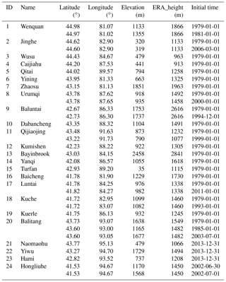
Table 1 Test sites information (ERA_height is the ERA-Interim grid height). The date format is year-month-day.

3.2 Observations

Daily air temperature records from 24 meteorological stations on the CTM from the China Meteorological Data Sharing Service System of the National Meteorological Information Center (CMA-CMDC, http://data.cma.cn/, last access: 16 November 2018) were used in the analysis. The observations include daily maximum temperature, minimum temperature, and mean temperature calculated from four observed records (6-hourly) from the previous 20:00 to the present 20:00 Beijing time. An overview of the observations is provided in Fig. 1 and Table 1. Some stations were relocated, which led to a different initial time (Table 1). The elevation was adjusted for station no. 24, but the coordinate was not changed. The quality of the observed data is strictly controlled by the National Meteorological Information Center of China. Therefore, 6-hourly ERA-Interim temperature is adjusted according to the time differences to match observations. Please note that only 7 out of the 24 meteorological stations are available for international users via the CMA-CMDC with registration. These 7 sites are a small part of the global exchange data set, which covers 194 sites starting during January 1951 over China for the global exchange program (http://data.cma.cn/en/?r=data/detail&dataCode=SURF_CLI_CHN_MUL_DAY_CES_V3.0, last access: 16 November 2018). These 7 sites are nos. 2, 5, 6, 8, 15, 18, and 23 in this study.

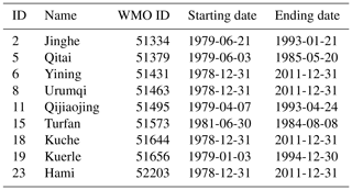
A very important but difficult to answer issue is that if some individual sites are assimilated by the ECMWF Integrated Forecast System, the ERA-interim predictions are not fully independent from the observed data which are subsequently used for calibration and validation. We investigated the ECMWF assimilation records and found that 9 of the 24 sites were possibly assimilated by the IFS. Table 2 shows the details of the assimilated sites. The long-term temperature records (1979–2011) from nos. 6, 8, 18, and 23 were assimilated. Only short-term observations (less than 15 years) from the other five sites were assimilated. According to the information from the ECMWF, it can be assumed that although 9 of the 24 sites were possibly assimilated, the other 15 sites were not used by ERA-Interim and therefore represent a fully independent data set. Furthermore, compared to the assimilated short-term observations, we tested a much longer time series. Thus, we cautiously believe that this issue does not affect the skill of ERA-Interim as well as the validation.

3.3 Elevation correction method

The original ERA-Interim temperature can be corrected via Eq. (1). T_{ERA_2m} is the original 6-hourly ERA-Interim 2 m temperature at a model height of a 0.25^∘ grid. The Γ value describes the lapse rate with a decrease in air temperature with elevation. The Δh value is the altitude difference between the 1 km digital elevation model (DEM) grid (resampled from 90 m of a Shuttle Radar Topography Mission (SRTM) DEM to 1 km) and the ERA-Interim grid model height.

$$\begin{array}{}\text{(1)}& T_i=T_{\mathrm{ERA}\mathrm{\_}\mathrm{2}\mathrm{m}}+\mathrm{\Gamma }\times \mathrm{\Delta }h\end{array}$$

Here, Γ represents the ERA-Interim internal lapse rates calculated from the temperatures and geopotential heights at different pressure levels. For example, Γ_{500_700} represents the temperature lapse rate between the 500 and 700 hPa pressure levels. Specifically, it is calculated by the temperature differences divided by height differences between the 500 and 700 hPa pressure levels. All variables and parameters are from ERA-Interim, which means this method is fully independent of observations. In the present study, Γ was defined according to the 1 km grid altitude. For example, if one 1 km DEM grid is 500 m in altitude, Γ_{850_925} will be applied based on the 850 and 925 hPa pressure levels, which represent an average height of 1500 and 150 m, respectively. If the DEM grid height is 4500 m, Γ_{500_600} between the 500 hPa (geopotential height ∼5000 m) and 600 hPa (geopotential height ∼4000 m) pressure levels will be used for the correction model. Normally, the zone higher than 4000 m in the CTM is mainly dominated by free airflow. In summary, Γ_{500_600}, Γ_{600_700}, Γ_{700_850}, and Γ_{850_925} were used for the DEM grids with heights of ≥4000, 3000–4000, 1500–3000, and ≤1500 m, respectively. More details regarding the correction method can be found in Gao et al. (2012, 2017).

Table 2 Assimilated sites in ERA-Interim. The date format is year-month-day.

3.4 Evaluation criteria

To evaluate the correction temperatures, two statistical accuracy measures were applied. The root-mean-square error (RMSE) was used for an assessment of the bias between the corrections and observations (Eq. 2). The Nash–Sutcliffe efficiency coefficient (NSE) evaluated the performance of the new data set using Eq. (3), which ranged from 1 (perfect fit) to minus infinity (worst fit) (Nash and Sutcliffe, 1970).

$$\begin{array}{}\text{(2)}& {\displaystyle }& {\displaystyle }\mathrm{RMSE}=\sqrt{{\displaystyle \frac{\mathrm{1}}{n}}\sum _{t=\mathrm{1}}^n{\left(T_{\mathrm{o}}-T_{\mathrm{d}}\right)}^{\mathrm{2}}},\text{(3)}& {\displaystyle }& {\displaystyle }\mathrm{NSE}=\mathrm{1}-{\displaystyle \frac{\sum _{t=\mathrm{1}}^n{\left(T_{\mathrm{o}}-T_{\mathrm{d}}\right)}^{\mathrm{2}}}{\sum _{t=\mathrm{1}}^n{\left(T_{\mathrm{o}}-\stackrel{\mathrm{‾}}{T_{\mathrm{o}}}\right)}^{\mathrm{2}}}},\end{array}$$

where T_o is the observed temperature at time t, T_d is the corrected temperature at time t, and n is the number of records in the same time series.

A measure of skill based on the probability density function (PDF) proposed by Perkins et al. (2007) was applied in this analysis. This skill score calculates the cumulative minimum intersections (or overlaps) between the two distribution binned values in the given PDFs. The skill score ranges from 0 to 1. A value of 1 means the PDF shape of the corrected temperature perfectly matched the observed PDF. The value 0 means there is no common area between the PDFs of observations and corrections. In other words, these two PDFs are completely independent. The PDF-based skill score was calculated via Eqs. (4) and (5):

$$\begin{array}{}\text{(4)}& {\displaystyle }& {\displaystyle }\mathrm{skill}\mathrm{score}=\sum _{\mathrm{1}}^m{P}_m,\text{(5)}& {\displaystyle }& {\displaystyle }{P}_m=\left\{\begin{array}{ll}{P}_{\mathrm{d}}^m,& P_{\mathrm{d}}^m<P_{\mathrm{o}}^m\\ P_{\mathrm{o}}^m,& P_{\mathrm{d}}^m\ge P_{\mathrm{o}}^m\end{array}(m=\mathrm{1},\mathrm{2},\mathrm{3}\mathrm{\dots }n),\right.\end{array}$$

where n is the number of bins for the PDF calculation, P_d is the frequency of values in a given bin from the corrected temperatures, and P_o is the frequency of the values in a given bin from the observations (Gao et al., 2016; Perkins et al., 2007). In this comparison, 1 ^∘C is used as the interval of bins for all the skill score calculations. The PDF-based evaluation method allows merging data from multiple stations across different time periods (Gao et al., 2016; Perkins et al., 2007). This evaluation method has been proven to show more credible climatic variations particularly for extreme values compared to those of the conventional mean-based assessment method (Gao et al., 2016; Mao et al., 2010). Furthermore, 1 % quantile and 5 % quantile temperatures are represented for extreme low temperatures, while 95 % quantile and 99 % quantile temperatures are selected for extreme high temperatures. A quantile function is more reliable than absolute minimum and maximum values, particularly for data sets in different time series. The corrected temperature is during the period of 1979–2016 and the observation is during the period of 1979–2013. These different durations of two data sets do not affect the comparison using a PDF-based skill score and quantile function.

Notably, the corrected temperature is accordingly averaged over nine grid points surrounding each meteorological station. This process was suggested by a referee when the authors evaluated the ERA-Interim temperature over the Tibetan Plateau (Gao et al., 2014a). The referee claimed that this approach can evaluate the ability of ERA-Interim over different topographies by selecting 3×3 grids with the station in the center grid. Thus, in this study we took this suggestion.

Here, we would like to emphasize that averaging nine grid points may lead to a systematic bias because the station elevation does not perfectly coincide with the mean elevation of the considered grid cells. However, the elevation differences among the averaged nine DEM grids and station elevations are quite small with an average of −8 m (Table S1 in the Supplement). Except for no. 9, the stations have less than a 50 m elevation difference. The elevation differences among the nine grids at a 1 km × 1 km grid resolution are very small (less than 2 m). From this point of view, a DEM generally matches the station elevations, and the systematic bias is very small. Thus, we believe this approach does not affect the validation.

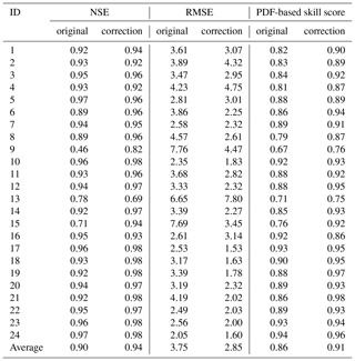
Table 3 Comparison of the original and corrected ERA-Interim temperature with daily observations. The NSE, PDF-based skill score, and RMSE in ^∘C are listed.

4 Results

4.1 Evaluation of original ERA-Interim temperature data

The correlation coefficient ranges from 0.949 to 0.995 with an average of 0.986 for all the stations (the detailed results not shown here). This high correlation coefficient indicates that the original ERA-Interim temperature captures the temporal variation in observations very well. However, the original ERA-Interim cannot capture the spatial characteristics at finer scales (Fig. S1). The very general spatial variation could be captured by the original ERA-Interim. The temperature is warmer in the lower basins in the southern and northern CTM and colder in the higher mountains in the central and western CTM. However, the temperature spatial variation is not captured at microtopographic scales because of the coarse resolution. The characteristics of temperature changes in the valleys and summits in the western and central CTM, such as the Ili River basin and Bogda Mountain, are not identified by the original ERA-Interim. This indicates that the original ERA-Interim is needed to correct for a finer spatial resolution. Table 3 shows a comparison of original ERA-Interim 2 m temperature data to daily observations from 24 meteorological stations. The NSE ranges from 0.46 to 0.97 for all stations. Only five stations (nos. 6, 8, 9, 13, and 15) have NSEs lower than 0.90. The average NSE of 0.90 for all stations shows that the ERA-Interim data reproduce observations very well. The lowest NSE is found at station no. 9 (Baluntai), while the highest NSE is found at no. 5 (Qitai) and no. 24 (Hongliuhe). The RMSE ranges from 2.05 to 7.76 ^∘C with an average of 3.75 ^∘C for all stations. Three stations (nos. 9, 13, and 15) have RMSEs higher than 5 ^∘C. As the NSE indicated, station no. 9 (Baluntai) has the largest RMSE (7.76 ^∘C), followed by station no. 15 (7.69 ^∘C). The smallest RMSE is found at station no. 24 (Hongliuhe).

Station no. 9 (Baluntai) is in a valley with an elevation of ∼1700 m, while the terrain height of the corresponding grid in ERA-Interim is 2616 m (Table 1). The approximate 900 m elevation difference may be responsible for the large RMSE. Station no. 13 (Bayinbrook) is in the hinterland of the CTM in the Kaidu River valley. The elevation difference between the site and the ERA-Interim grid is 383 m, which partly accounts for the large RMSE. Station no. 15 (Turfan) is in a basin on the southern hillside of the CTM at an elevation of only 35 m. The ERA-Interim grid height (1115 m) is much higher than the site, which may lead to a large bias. Figure 2 shows the comparison of observational and original ERA-Interim temperature data at station nos. 10, 24, 9, and 15. The ERA-Interim estimates both lower and higher temperatures quite well at station nos. 10 and 24 (Fig. 2a and b). The ERA-Interim underestimates observations for station nos. 9 and 15 because of their higher grid elevation, particularly for higher temperatures (Fig. 2c and d).

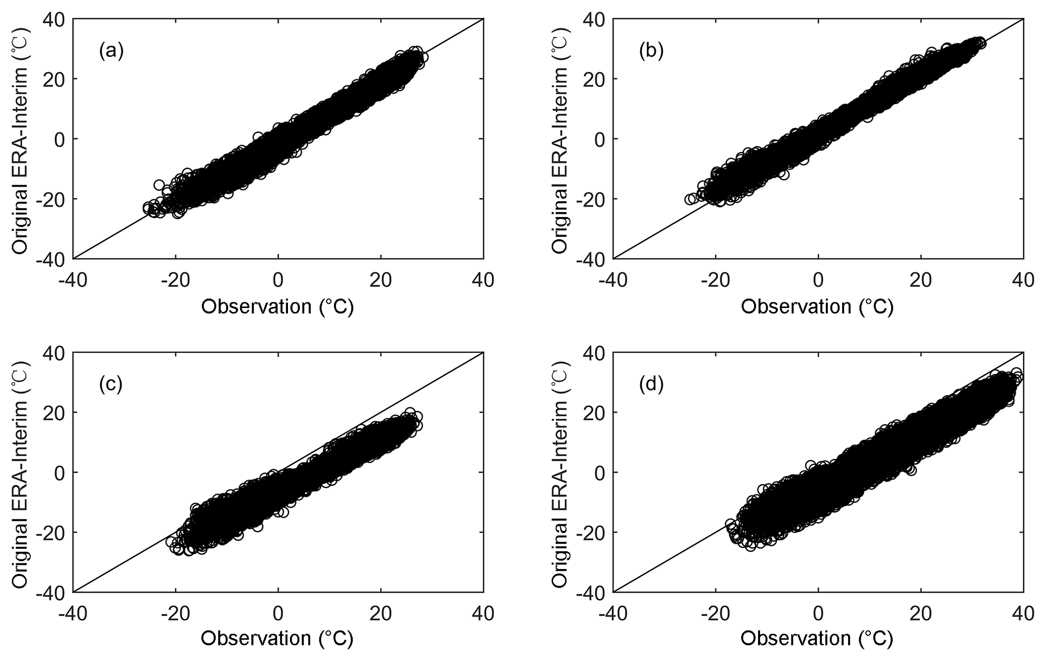
Figure 2 Scatter plots of observation and original ERA-Interim temperature data for (a) station no. 10, (b) station no. 24, (c) station no. 9, and (d) station no. 15. The corresponding RMSEs can be found in Table 3.

Figure 3 Probability density functions for observation, original ERA-Interim, and corrected ERA-Interim for (a) station no. 10, (b) station no. 24, (c) station no. 9, and (d) station no. 15. The corresponding PDF-based skill score can be found in Table 3.

The PDF-based skill score ranges from 0.67 to 0.94 with an average of 0.86 for all stations. Four stations (nos. 8, 9, 13, and 15) have skill scores less than 0.8. The highest skill score is found at station no. 24, while the smallest is found at station no. 9. Figure 3 shows greater detail particularly in terms of the temperature bins of the PDFs, which could help to easily identify how well ERA-Interim estimates lower and higher temperatures. For station no. 10, the original ERA-Interim captures the shape of the observed PDF very well, particularly in the range of 0–15 ^∘C. In the range of −10–0 ^∘C and higher than 20 ^∘C, the observed probability is higher than that of the original ERA-Interim. However, the probability of the original ERA-Interim is higher than that for observations at lower temperatures ($<-\mathrm{10}$ ^∘C). For station no. 24, the original ERA-Interim fits the shape of the observed PDF very well nearly for the entire temperature range. It only has a lower probability for temperatures lower than −10 ^∘C. For higher temperatures (>20 ^∘C), the probability of the original ERA-Interim is slightly higher than that for observation. For station no. 9, the shape of the PDF from original ERA-Interim is higher (higher probability) for the temperatures lower than 12 ^∘C and is lower (lower probability) for the temperatures higher than 12 ^∘C compared to the observed PDF. For station no. 15, the original ERA-Interim does not generally match the shape of observed PDF. The probability of the original ERA-Interim is much higher than that for the observational data for temperatures cooler than approximately 25 ^∘C, while it is much lower than that of the observational data for higher temperatures (>25 ^∘C). The aforementioned analysis indicates that although the original ERA-Interim captures the temporal variation in the observations very well, the large RMSE and poor performance for extreme temperatures suggest that a correction process of ERA-Interim is necessary for application at individual sites.

4.2 Temporal variability of lapse rates

Lapse rate shows the empirical relationship between temperature and altitude. However, it significantly changes over a short time and distance, particularly in a valley during winter, in which the lapse rate could reverse (Li et al., 2015). Previous studies (Gao et al., 2012, 2017) have tested the ERA-Interim internal lapse rates in the German and Swiss Alps as well as on the Tibetan Plateau. The results showed that in general the internal lapse rates could capture the variability in the observed lapse rates, although the performances were different for the different grid cells (large spatial variation). To illustrate the reliability of the ERA-Interim lapse rates in the CTM, Γ_{700_925} was calculated to compare to the observed lapse rate for the 24 sites. In previous studies (Gao et al., 2012, 2017), the observed lapse rate was calculated from two or three sites within the same ERA-Interim grid. Unfortunately, the sparse station distribution cannot support this calculation in the CTM. Thus, we investigate the lapse rate based on the temperature and elevational information from all 24 sites using a linear regression from 1979 to 2013. To ensure the site elevations (ranging from 35 to 2458 m) are in accordance with the ERA-Interim pressure height, Γ_{700_925} was calculated using the temperature and geopotential height at the 925 hPa (∼150 m) and 700 hPa (∼3000 m) pressure levels. Subsequently, the monthly lapse rates for the observational and ERA-Interim data from 1979 to 2013 were calculated, respectively.

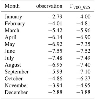
Figure 4 shows the temporal variability in the monthly lapse rates. In general, ERA-Interim (Γ_{700_925}) has a higher temperature gradient than that of the observation for the whole year. However, Γ_{700_925} captures the variability in observed lapse rate very well, particularly during the warmer months (May to August). The inter-monthly variability in the observed lapse rate is much higher than Γ_{700_925}, particularly from September to January. The temperature gradient significantly decreases from September onward, which represents the transition month from a warm to cold climatic regime. The temperature gradient significantly increases from March onward, which represents a climatic regime transfer from cold to warm conditions. Table 4 shows the average monthly lapse rates for all 24 sites during the period of 1979–2013. The lapse rate differences are small (less than 0.5 ^∘C km⁻¹) from May to August, while the differences are greater than 1 ^∘C km⁻¹ from September to December and during January.

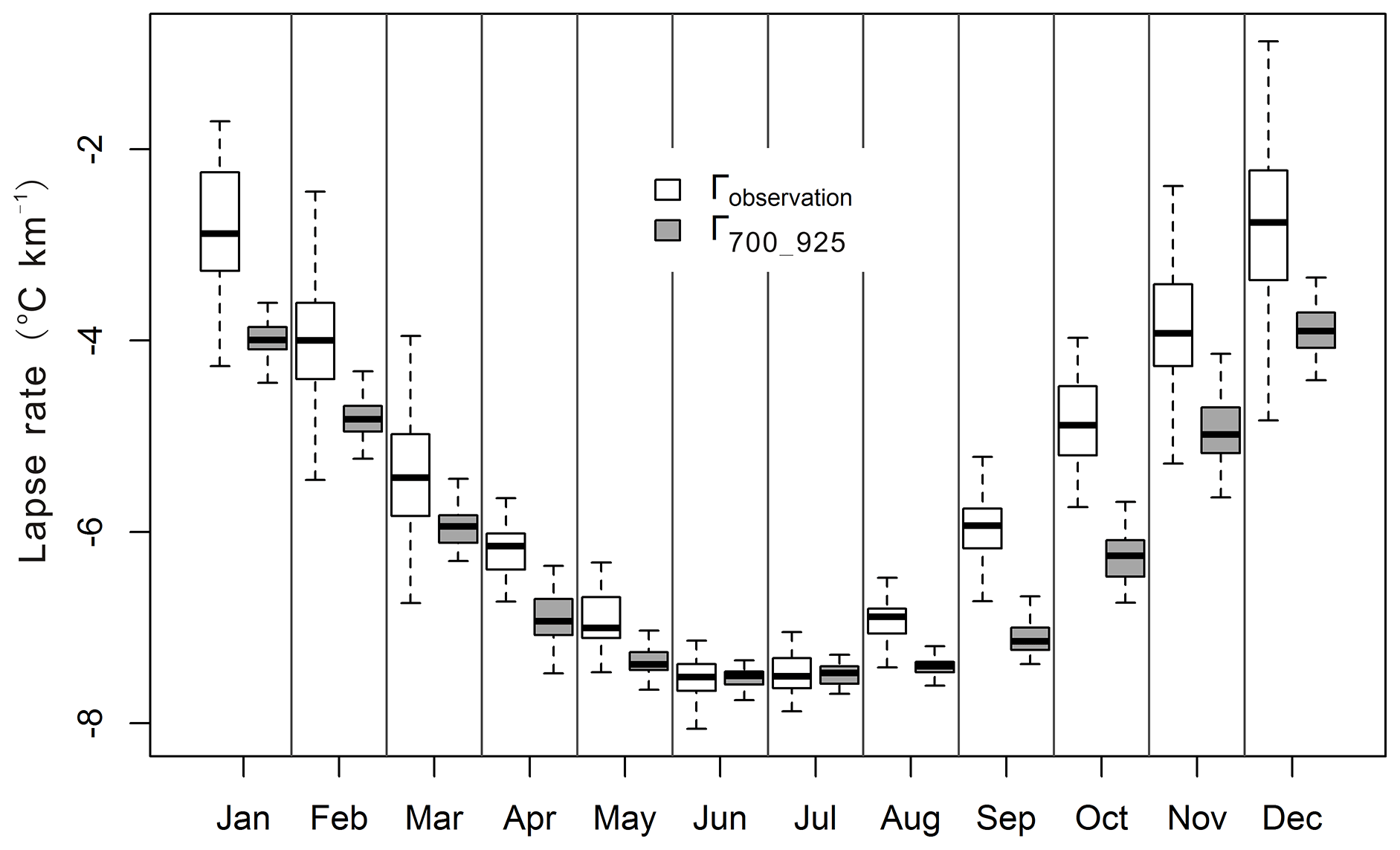
Figure 4 Box plots of monthly lapse rates for observation and ERA-Interim (Γ_{700_925}). Thick horizontal lines in boxes show the median values. Boxes indicate the inner-quantile range (25 % to 75 %) and the whiskers show the full range of the values.

In order to evaluate the intra-seasonal variations of lapse rate, the correlation between observed and modeled lapse rates for each month and season were analyzed (Table S4). The correlation ranges from 0.25 to 0.74 with an average of 0.45. The seasonal correlation is 0.62, 0.43, 0.41, and 0.32 for spring, summer, autumn, and winter, respectively. Except for April, May, and September, the correlation is lower than 0.5 for other months. Only spring has a higher correlation than 0.6 compared to other seasons. Although, the correlation is at a low level, it does not mean that the lapse rate of ERA-Interim does not work. There are several reasons for the nonsignificant statistical correlation. Firstly, the observed lapse rate was from the linear regression based on 24 sites. Secondly, the time series is only 35 years, which is relatively short for a temporal correlation analysis. The best way to compare observed and model lapse rate is the approach in Gao et al. (2012, 2017), which compared the two lapse rates in the same ERA-Interim grid cell. However, this analysis further indicates that more observations are really needed for evaluation.

4.3 Validation of corrected ERA-Interim temperature data

The average correlation coefficient changes from 0.986 to 0.987 for all stations (not shown here) with respect to the original and corrected ERA-Interim temperature data. Table 3 shows a comparison of corrected ERA-Interim 2 m temperature with daily observations from 24 meteorological stations. The NSE for the corrected ERA-Interim ranges from 0.69 to 0.98 for all sites. The average NSE enhances by 5 % from 0.90 to 0.94. The NSE significantly increases from 0.46 to 0.82 for station no. 9 and from 0.71 to 0.94 for station no. 15. Applying the elevation correction framework does not lead to an increased NSE at station nos. 2, 4, 5, and 13, particularly for station no. 13 (Bayinbrook). This indicates that other factors also affect the temperature changes, not only altitude. The RMSE of the corrected ERA-Interim changes is from 1.53 to 7.80 ^∘C. An average 0.9 ^∘C (24 %) RMSE is reduced from 3.75 to 2.85 ^∘C. The RMSE reduces at all sites except nos. 2, 4, 5, 13, and 16. The RMSE increases approximately 0.5 ^∘C for station nos. 2, 4, 5, and 16. RMSE increased by 1.15 ^∘C for station no. 13. RMSE reduced by 42 % and 55 % for station nos. 9 and 15, respectively. A total of 16 out of the 24 sites have RMSEs lower than 3.0 ^∘C following the correction process. Figure 5 shows a comparison of observational and corrected ERA-Interim temperature data at station nos. 9, 10, 15, and 24. The scatter plot shows a slight improvement (for higher temperature) at station nos. 10 and 24 compared to the original ERA-Interim data (Figs. 2 and 5). However, the scatter plot is more concentrated along the 1 : 1 line for station no. 9 and particularly no. 15 (Fig. 5c and d), which suggests that the correction procedure works well at these two stations.

Table 4 Average monthly lapse rates (^∘C km⁻¹) for the 24 sites in 1979–2013.

Temperature significantly varies during different seasons and different times of the day because of complex topography. For example, during the winter nights, the lapse rate possibly reverses (local inversion) from the bottom of the valley to the high mountains because of a “cold lake” (Gerlitz et al., 2014). To identify the limitations for end users, we tested the seasonal bias using the 24 sites. Table 5 shows the RMSE of the seasonal mean temperatures between the original ERA-Interim and corrected temperatures for all sites. The RMSE for spring ranges from 0.26 to 4.22 ^∘C with an average of 1.24 ^∘C. The performance for summer and autumn is similar at an approximately 1.4 ^∘C RMSE. Winter has the largest average RMSE (2.96 ^∘C) during the year. Different stations show significantly different performance. For example, station no. 13 shows the largest RMSE for winter and the smallest RMSE for summer. Station no. 9 shows the opposite performance, in that the summer has the largest RMSE (5.47 ^∘C) while the winter has the smallest RMSE (2.32 ^∘C). This further illustrates that the complex terrain of the CTM leads to complexity and diversity in climate. In general, the warmer season (May to September) is much better than the colder months.

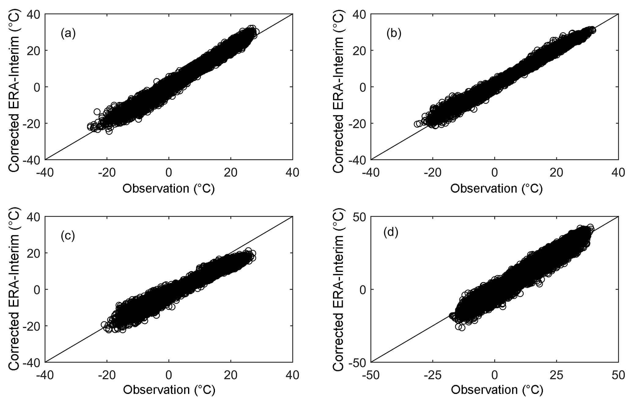
Figure 5 Scatter plots of observation and corrected ERA-Interim temperature data for (a) station no. 10, (b) station no. 24, (c) station no. 9 and (d) station no. 15. The corresponding RMSE can be found in Table 3.

The average PDF-based skill score increases from 0.86 to 0.91 for all stations (Table 3). The correction results show better probability distribution functions compared to the original ERA-Interim for all stations except no. 16 (Baicheng). Although five stations have increased RMSEs, the PDF-based skill score enhances at four of the five stations (station nos. 2, 4, 5, and 13). This indicates that the correction procedure reduces the PDF discrepancy between the original ERA-Interim and observational data. Figure 3 shows more details regarding correction performances for the four representative stations. For station no. 10, the PDF curve of the corrected ERA-Interim shifts right compared to that of the original, and it perfectly fits with observed PDF in a range of temperatures lower than −8 ^∘C. The probability of the corrected ERA-Interim is less than that of the observation at temperatures between −8 and 22 ^∘C (Fig. 3a). For station no. 24, the PDF shape of the corrected ERA-Interim shifts slightly left against the original and fits the observed PDF much better for temperatures higher than 0 ^∘C (Fig. 3b). For station no. 9, the probability of the corrected ERA-Interim is much higher than that of the observed temperature at a temperature lower than 15 ^∘C, particularly in the range of 0–15 ^∘C. It performs better than the original ERA-Interim for higher temperatures (>15 ^∘C). A much better agreement between the PDF curves of the corrected ERA-Interim and observational data is found at station no. 15 (Fig. 3d). The probability of the corrected ERA-Interim is much nearer the observational data compared to that of the original ERA-Interim in the range of 15–35 ^∘C. The correction procedure reduces a significant PDF discrepancy for station no. 15, which lies at a lower elevation (35 m). The validation suggests that the correction method is generally reliable and it could significantly reduce the RMSE and PDF discrepancy for most of the stations, although it does not perform well for some individual sites.

Table 5 RMSEs of seasonal temperatures between the original ERA-Interim and corrections for the 24 sites in 1979–2013.

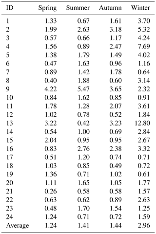
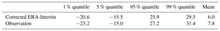
Table 6 Climatology of the entire CTM based on corrected ERA-Interim temperatures (1 km, 6-hourly, 1979–2016) and daily observations (daily, 1979–2013, ^∘C).

In order to evaluate whether the elevation correction approach captures important characteristics and processes in similar environments, the 24 sites were divided into 5 groups in different elevation ranges: 0–500 m (nos. 2, 3, 4, 15, 21), 500–1000 m (nos. 5, 6, 8, 11, 12, 17, 19, 23), 1000–1500 m (nos. 1, 10, 14, 16, 18), 1500–2000 m (nos. 7, 9, 20, 22, 24), and 2000–2500 m (no.13). The averaged NSE, RMSE, and PDF-based skill scores for different elevation groups were analyzed. Table S2 shows the averaged NSE, RMSE, and PDF-based skill scores between the original and corrected ERA-Interim temperatures for different elevation groups. Except the highest elevation group (2000–2500 m), NSE enhances and RMSE decreases significantly after elevation correction for other groups. However, it is arbitrary to judge that the correction method does not work for higher elevation sites. There are two main possible reasons. Firstly, there is only one site in this group (no. 13), which is not enough to evaluate the performance of correction method. Actually, Gao et al. (2012) showed that the higher sites (e.g., Zugspitze site, 2964 m) were better compared to the ground site. Secondly, the local topographical characteristics may affect the temperature changes at site no. 13. Table S3 shows the averaged RMSEs of seasonal temperatures between the original ERA-Interim and corrections for different elevation groups. Winter has the largest RMSE for the sites lower than 1500 m. These three groups applied the lapse rate Γ_{850_925}. RMSEs are relatively smaller than 1.5 ^∘C for these sites in spring, summer, and autumn. The group of 1500–2000 m has RMSEs lower than 2 ^∘C for the seasons. Again, the highest group (no. 13) has the largest RMSE for spring, autumn, and especially winter. However, it has the best performance for summer. Table 4 and Fig. 4 have shown an almost perfect lapse rate against observation. However, the mechanism of temperature changes in the winter should be further investigated.

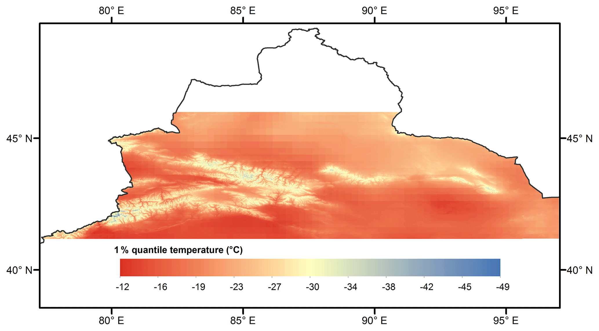
Figure 6 The 1 % quantile temperature of the entire CTM based on the high-resolution data set.

Figure 7 The 99 % quantile temperature of the entire CTM based on the high-resolution data set.

Figure 8 Mean temperature of the entire CTM based on the high-resolution data set.

4.4 Climatology of the Chinese Tian Shan based on the high-resolution data set

The low density of meteorological stations in the CTM may lead to uncertainty in the representation of the entire area's temperature climatology. Interpolation also carries a risk in representing the climatology because it is based on meteorological stations. Here, the entire area's climatology was investigated using the corrected high-resolution data set from 1979 to 2016. Quantile temperature is more reliable than absolute minimum and maximum temperatures if an outlier exists. Thus, the 1 % quantile and 99 % quantile of the long-term series were selected to represent the extreme cold and hot temperatures, respectively. Figure 6 shows a new comprehensive climatology of the extreme low temperature over the CTM based on the corrected ERA-Interim temperature data. The 1 % quantile temperature ranges from −49 to −12 ^∘C, which is consistent with the topography. The lower temperatures could be found at the Borokoonu, Bogda, and Khark mountains. The extreme cold temperatures ($<-\mathrm{40}$ ^∘C) are on the Tomur, Bogda, and Tianger peaks. The higher temperatures could be found in the Ili River valley and Junggar, Turfan, Hami, and Tarim basins. The extreme hot temperatures are found at the border of the Ili River valley and the western Tarim Basin.

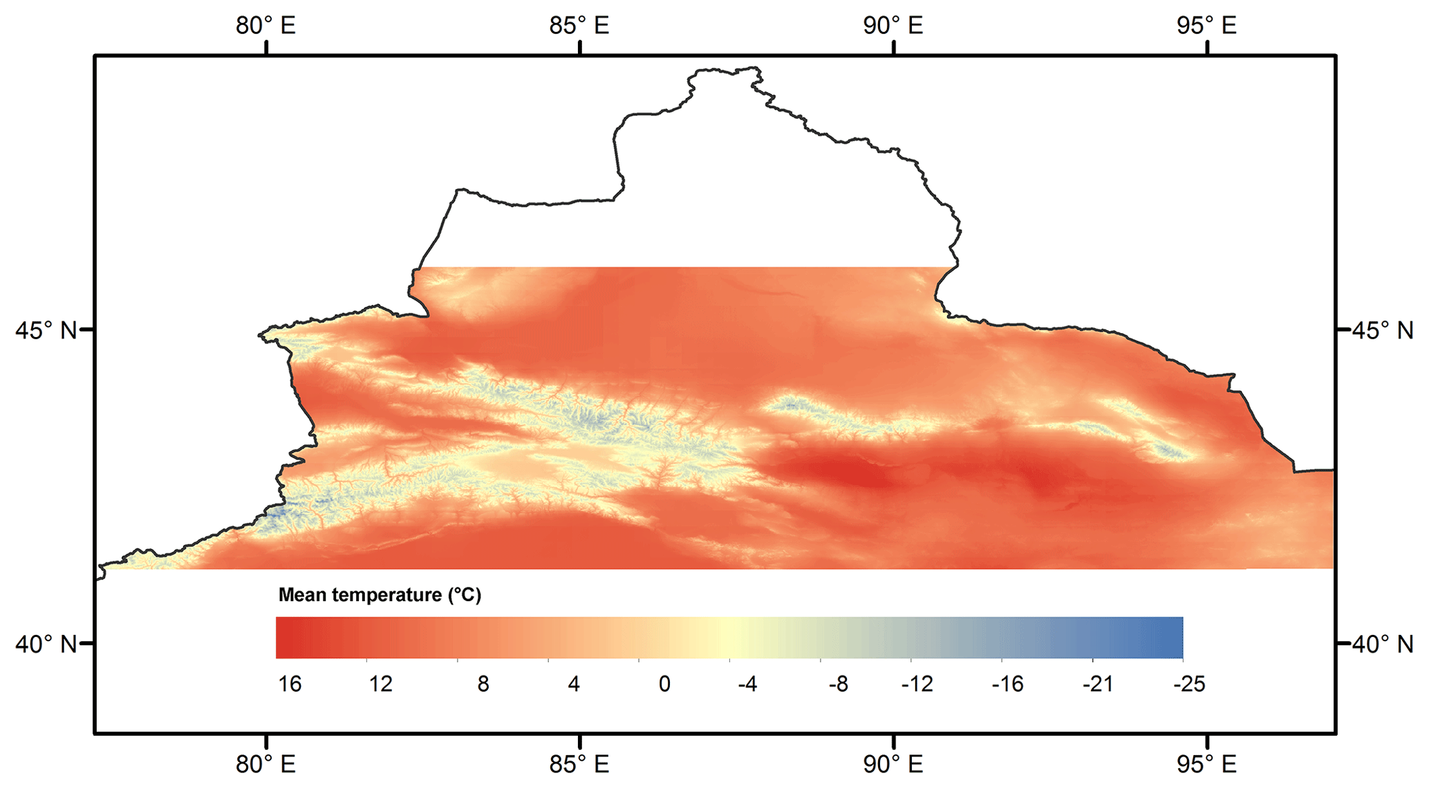
Figure 7 shows the 99 % quantile temperature which represents the extreme warm temperature in the CTM. The Turfan Basin and Hami Basin are the hottest areas over the entire CTM. The highest temperature can reach 45 ^∘C. The temperature in the high mountain areas such as Tomur Peak and Bogda Peak can be higher than 0 ^∘C. The minimum temperature of the 99 % quantile is approximately −3 ^∘C. Figure 8 shows the mean temperature in the CTM. The temperature ranges from −25 to 16 ^∘C. The mean temperature distribution is consistent with extreme cold and hot temperatures. It suggests that the topography has a significant impact on temperature.

Table 6 illustrates a climatological comparison for the entire CTM using corrected ERA-Interim temperature and 24 stations. The 1 % and 5 % quantile were selected to represent the colder temperatures while the 95 % and 99 % quantiles for the higher temperatures. Please note that these two data sets (corrections and observations) have different spatial resolution and time series and thus sample numbers. However, this does not affect the general climatological comparison very much. The new data set underestimates the observations except for the 1 % quantile, which suggests that it may be warmer than the observation during the cold season. Only a 0.5 ^∘C difference was found between the two data sets for the 5 % quantile. Temperatures of 1.3, 1.9, and 1.8 ^∘C were the underestimates by the new data set for the 95 % quantile, 95 % quantile, and mean temperature, respectively. It can be concluded that the new data set could generally capture the climatology of the entire CTM, particularly for warmer temperatures. Some researchers are more interested in maximum and minimum temperatures rather than 1 % and 99 % quantiles. Thus, the figures for spatial distribution of the maximum and minimum temperatures over the CTM are also provided in the Supplement (Figs. S2 and S3).

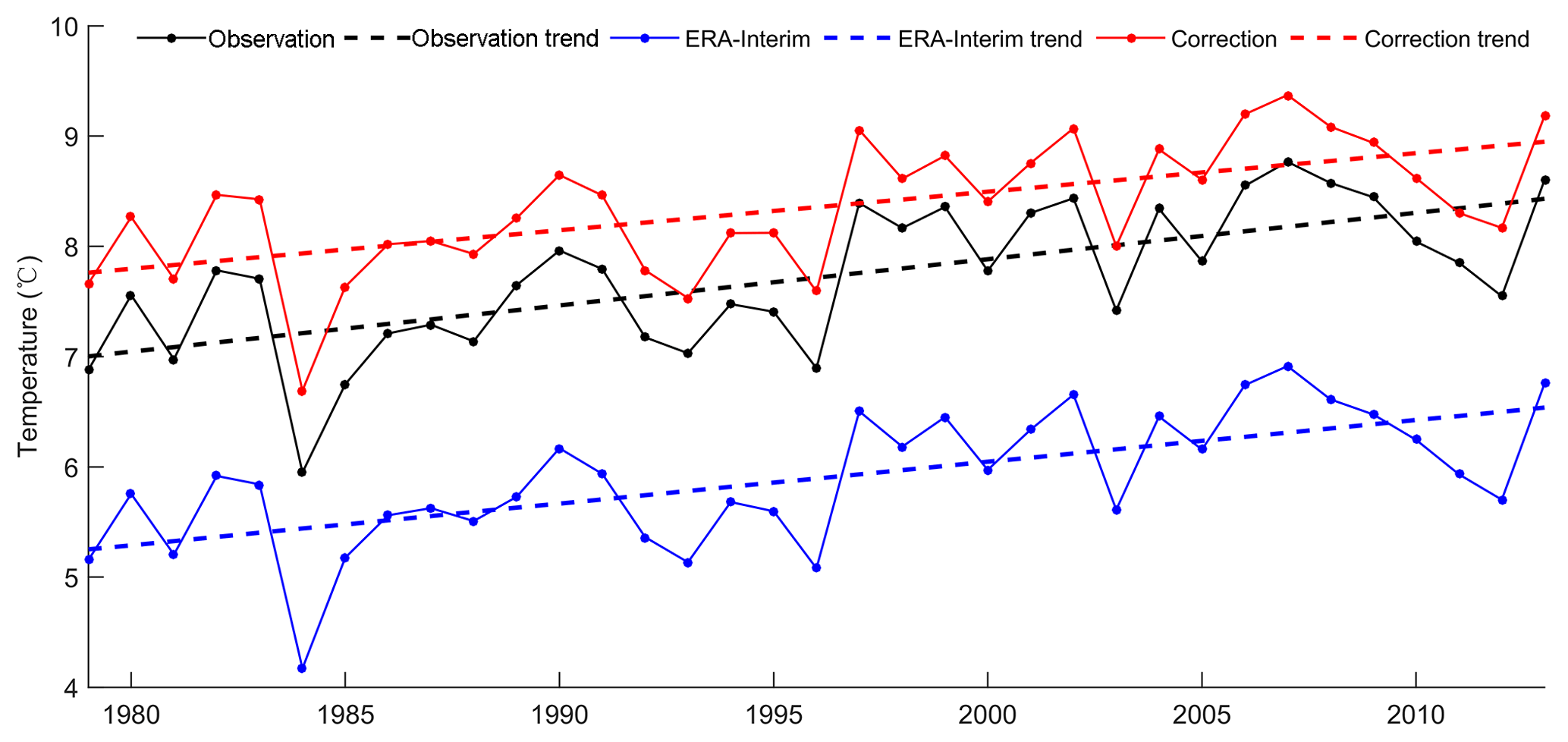
Figure 9 Temporal variations of annual temperatures for observation, original ERA-Interim, and the correction temperatures for the 24 sites in 1979–2013.

4.5 Trends of the annual and seasonal T_max, T_min, and diurnal temperature range (DTR) in the CTM

Previous studies have shown that the elevation dependent warming trend and the spatial and seasonal variations in the diurnal temperature range are very important features for an alpine climate (Gerlitz, 2014; Gerlitz et al., 2014; Sun et al., 2018; Shekhar et al., 2018). To better illustrate the limitations of the new data set, the daily maximum temperature (T_max), daily minimum temperature (T_min), and diurnal temperature range (DTR) from the original ERA-Interim and the corrected temperatures for the 24 sites during the period of 1979–2013 were analyzed.

Figure 10 Temporal variations of T_max from observation, original ERA-Interim, and correction temperatures for the 24 sites in 1979–2013.

The warming trends of observation, original ERA-Interim, and correction temperatures for the 24 sites during the period of 1979–2013 were compared (Fig. 9, Table 7). The original ERA-Interim significantly underestimated (approximately 2 ^∘C) the observations. However, the corrections overestimated by approximately 1 ^∘C. An annual warming trend with an increase rate of 0.420 ^∘C 10 a⁻¹ was found for the observation. Generally, the original ERA-Interim and corrected temperatures capture the warming trend very well with a rate of 0.378 and 0.349 ^∘C 10 a⁻¹, respectively. Table 7 shows the trends in seasonal temperatures for the 24 sites during the period of 1979–2013. Spring has the largest positive trend with a rate of 0.664 ^∘C 10 a⁻¹. The original ERA-Interim and corrected temperatures captured the warming trends for spring quite well with a rate of 0.659 and 0.638 ^∘C 10 a⁻¹, respectively. The correction temperatures showed better performance than the original ERA-Interim during summer. However, the ERA-Interim and corrections both underestimated the trend with nearly the same rate for the autumn trend. Unfortunately, the slight positive warming trend during winter is not captured by the original ERA-Interim and correction temperatures. These two data sets show similar negative trends.

Table 7 Trends (^∘C 10 a⁻¹) of annual and seasonal temperatures over the 24 sites in 1979–2013.

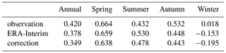
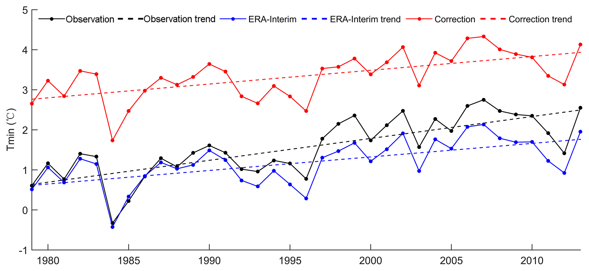
Figure 11 Temporal variations of T_min from observation, original ERA-Interim, and correction temperatures for the 24 sites in 1979–2013.

Figure 10 shows the temporal variations in T_max for the 24 sites during the period of 1979–2013. The bias of ERA-Interim is approximately 4 ^∘C compared to that of the observations. The corrections have a bias of less than 2 ^∘C. The variations are consistent with the similar warming trend. Table 8 shows the trends for seasonal T_max for the 24 sites during the period of 1979–2013. In general, the original ERA-Interim and corrections capture the warming trend quite well (∼0.370 ^∘C 10 a⁻¹). Observational data have the largest positive trend during spring with a rate of 0.693 ^∘C 10 a⁻¹, followed by autumn (0.528 ^∘C 10 a⁻¹). The warming trends are slightly overestimated by ERA-Interim and corrections during the summer. The original ERA-Interim and corrections capture the negative trend for winter, but at a higher magnitude than that of the observations.

Table 8 Trends (^∘C 10 a⁻¹) of annual and seasonal T_max over the 24 sites in 1979–2013.

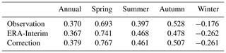
Figure 11 demonstrates the temporal variations in T_min for the 24 sites during the period of 1979–2013. The original ERA-Interim agrees with the observations very well at less than 1 ^∘C. The corrections have a bias of approximately 2 ^∘C compared to the observations. The original ERA-Interim and corrections underestimate the observed warming trend. Table 9 shows the specific values of the trends for seasonal T_min for the 24 sites during the period of 1979–2013. In general, the original ERA-Interim and corrections capture the warming trends for spring, summer, and autumn with lower rates, particularly for spring and autumn (Table 8). Observational data have the largest positive trend during spring with a rate of 0.700 ^∘C 10 a⁻¹, followed by autumn (0.661 ^∘C 10 a⁻¹). The observed warming trend for winter is positive with a rate of 0.209 ^∘C 10 a⁻¹. However, the ERA-Interim and corrections did not capture the positive trend.

Table 9 Trends (^∘C 10 a⁻¹) of annual and seasonal T_min over the 24 sites in 1979–2013.

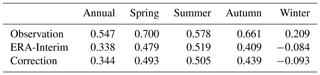
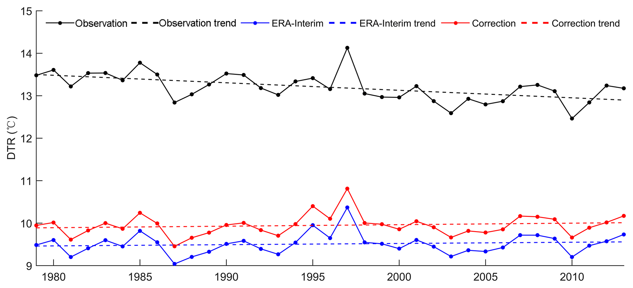
Figure 12 Temporal variations of DTR from observation, original ERA-Interim and correction temperatures for the 24 sites in 1979–2013.

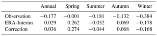
Figure 12 demonstrates the temporal variations in DTR for the 24 sites during the period of 1979–2013. The original ERA-Interim has a bias greater than 3 ^∘C DTR compared to that of the observations. The corrections reduce the DTR bias nonsignificance. The original ERA-Interim and corrections did not capture the significant decreasing trend of the DTR. Table 10 shows the specific values of the trends for seasonal DTR for the 24 sites during the period of 1979–2013. Decreasing trends are observed for annual and for seasonal DTR. Winter shows the largest decreasing rate at −0.384 ^∘C 10 a⁻¹. Spring shows an nonsignificant decreasing trend (−0.001 ^∘C 10 a⁻¹), which may result from the significant increasing rate of T_max. The original ERA-Interim and corrections capture the decreasing trends for summer and winter at smaller rates. However, they capture opposite trends for spring and autumn, particularly for spring (Table 10). The main reason is that the increasing rates for spring T_min are significantly underestimated by the original ERA-Interim and corrections (Table 9).

We would like to emphasize that we compared the DTR to the 24 observations rather than over the whole CTM. An analysis of the T_max, T_min, and DTR shows that the corrections can generally capture the annual trend, although not well at a seasonal scale. However, it is true that we need more observations to validate the performance of the new data set on DTR and spatial variations at local scales. At present, we are collecting more local observations from the CMA, particularly for specific subregions (for example, the Kaidu River basin) of interest to researchers.

Table 10 Trends (^∘C 10 a⁻¹) of annual and seasonal DTR over the 24 sites in 1979–2013.

5 Data availability

The data set presented in this article is published in the Network Common Data Form (NetCDF) at https://doi.org/10.1594/PANGAEA.887700 (Gao, 2018). The coverage of the data set is 41.1814–45.9945^∘ N, 77.3484–96.9989^∘ E. The grid point was derived from an SRTM DEM, which was resampled from 90 m to 1 km. The total number of grid points is 818 126. The time step is 6-hourly at 00:00, 06:00, 12:00, and 18:00 UTC. The time series is from 1979 to 2016. To reduce the size of each file, the grid points (818 126) are divided into 41 groups. Thus, each nc file contains 20 000 grid points, which is according to the grid point ID (see grid_points.nc). The time series also is divided into 5 years. The nc file name specifically shows the data information. For example, t2m_1979_1984_1_20000.nc means t2m_“beginning year”_“ending year”_“beginning grid point”_“ending grid point”.nc. The total number of nc files is 288. The disk usage of the data set is approximately 187 GB. Users can access the data via the DOI link to the PANGAEA web page (view data set as HTML under the Download Data item) by completing the following steps. (1) Download the grid_points.nc file, and then select the grid points for the target study area according to the coordinates. For example, a study area covers grid point IDs from 200 to 1000 and 14 000 to 25 000. The time series is supposed to be 1985 to 1989. (2) Download the data files t2m_1985_1989_1_20000.nc and t2m_1985_1989_20001_40000.nc. (3) Extract the temperature data according to the grid point IDs. (4) Analyze the data and plot figures. The data set that is organized in a monthly format (each month with all points in one nc file) will be accessible at PANGAEA in the future.

ERA-Interim data were supported by the ECMWF (https://www.ecmwf.int/en/forecasts/datasets/archive-datasets/reanalysis-datasets/era-interim/, last access: 16 November 2018). The meteorological data have been provided by China Meteorological Data Sharing Service System of the National Meteorological Information Center (http://data.cma.cn/, last access: 16 November 2018). The 7 out of 24 sites for global exchange are provided by CMDC (http://data.cma.cn/en/?r=data/detail&dataCode=SURF_CLI_CHN_MUL_DAY_CES_V3.0, last access: 16 November 2018).

6 Discussion and conclusion

Although the average temporal correlation (R=0.986) between the ERA-Interim and observations over the CTM is encouraging, an average RMSE of 3.75 ^∘C suggests that a correction process for ERA-Interim data is needed. Many factors may lead to errors, such as assimilated observational errors, the model background and operator errors in the ECMWF system. However, previous studies have shown that the elevation difference between the ERA-Interim grid and the individual site is a key factor for errors in high mountains such as the European Alps and on the Tibetan Plateau (Gao et al., 2012, 2014a, 2017). Therefore, it is possible to reduce such errors as well as correct (downscale) the grid value to a finer local scale using elevation-based methods.

Gao et al. (2012, 2017) claimed that the elevation correction method based on ERA-Interim internal, vertical lapse rates outperformed several conventional methods such as the use of fixed monthly lapse rates and observed lapse rates from meteorological stations in the European Alps and on the Tibetan Plateau. The performances were similar to the internal ERA-Interim vertical lapse rates derived from different pressure levels in the European Alps (Gao et al., 2012). Among these methods, using the lapse rate calculated from the pressure levels covering the highest and lowest meteorological stations has proven to be more accurate on the Tibetan Plateau (Gao et al., 2017). The most prominent advantage is that this method is fully independent from the observed data. Therefore, it provides a possibility to extrapolate ERA-Interim temperature data to any other high mountainous areas where no measurements exist.

Based on this hypothesis, the $\mathrm{0.25}{}^{\circ }\times \mathrm{0.25}{}^{\circ }$, 6-hourly ERA-Interim 2 m temperature data were corrected (downscaled) to a 1 km grid from 1979 to 2016 in the CTM, where there is serious lack of long-term temperature observations. To our knowledge, the presented data are the first data set (version 1.0) with high spatiotemporal resolution over such a long-term series for this region. To evaluate the quality of the new data set, observations from 24 meteorological stations were used for comparison. The average NSE was enhanced by 5 % from 0.90 to 0.94, and the average 0.9 ^∘C (24 %) RMSE was reduced from 3.75 to 2.85 ^∘C. The average PDF-based skill score increased from 0.86 to 0.91 after correction for all test sites. Except for a few sites, the correction method showed good performance for most of the sites, particularly for the site in the valley (no. 16 Baicheng). The PDF shape of the new high-resolution grid data fits the observed PDF much better in comparison to that of the original ERA-Interim temperature data. The validation indicates that the correction method is reliable and the RMSE and PDF discrepancy is significantly reduced for most stations.

The new data set captures the climatology of the entire CTM very well. It seizes the distribution characteristics, such as high temperature in the river valleys and basins and low temperature on the peaks. The bias is only 1.8 ^∘C between the corrected and observational values. Except for extreme cold temperatures, the new data set has a bias of less than 2 ^∘C compared to observations. In general, the corrected data set is appropriate for climate impact assessment and has the potential to be used for hydrological and environmental modeling. In general, the corrections capture the warming trend of annual mean temperature well (0.349 ^∘C 10 a⁻¹) compared to the observations (0.420 ^∘C 10 a⁻¹), except during winter. The corrections capture the T_max warming trend best for the annual and seasonal temperatures (∼0.370 ^∘C 10 a⁻¹). However, the new data set underestimates the T_min trend compared to the observations, particularly the opposite trend during winter. It also fails to reproduce the DTR trend for annual, spring, and autumn with a reverse trend. This indicates that the temperature significantly changes during winter. A temperature inversion layer may occur during the winter night in the valleys.

Certainly, some issues regarding the quality of the data set as well as the validation should be addressed here. The main hypothesis is that elevation plays the crucial role in temperature changes. This means that the temperature changes follow the lapse rate law in the vertical direction. However, in the horizontal direction, microtopographical features, such as aspect and mountain slope, possibly affect the temperatures in a short time. Temperature can be significantly different on a shady slope and a sunny slope. The lapse rate can sharply change or even inverse during the cold winter. This might be the main reason for the failure of the correction method at some sites, particularly during winter (e.g., no. 16 Baicheng). Figures 10, 11, and 12 have shown that the new data set still has a relatively large warm and cold bias (around 2 ^∘C) for T_min and T_max. The DTR is also underestimated. The potential users should be careful if they want to investigate the minimum and maximum temperature changes for complex regions, especially for winter. At present, T_min, T_max, and DTR are evaluated only at sites. The performances at subregions will be investigated to explore the mechanisms of local temperature changes with respect to microtopography characteristics such as aspect and slope based on more observations in the ongoing research. The grid height of the data set was derived from an SRTM DEM, which was resampled from 90 m to 1 km. As shown in Fig. 1, the highest altitude from the resampled SRTM is approximately 7100 m, which is approximately 300 m lower than the highest peak (Mount Tomur, 7443.8 m) in the CTM. Therefore, DEM bias may lead to a systematic error compared to observations. The number of meteorological stations for validation here was limited to 24. These stations are mainly in valleys and basins. Thus, it is difficult to evaluate the credibility of the data set in the high mountains where more glaciers occur. Other observational resources, such as remote-sensing data, are helpful for further validation. We are attempting to collect and apply more observations from the CMA to validate the new data set. However, at present, we have used the best available. We expect other researchers to validate our product using different data resources. More validation and applications are welcome. Because of the limitation in computational resources and the accessibility of data sources (only 6-hourly ERA-Interim temperature data are open access to the public), the resolution of this data set is limited to 6-hourly and 1 km grid spacing. However, the current data set (∼187 GB) is huge to process and store. The computational resource and disk usage of the data set will exponentially increase when the spatiotemporal resolution increases. For such a huge amount of data, storage and extraction are not convenient. Supercomputers and parallel computing are necessary in the future. Higher resolution, more validation, and correction method improvement (version 2.0) are topics of ongoing and future research.

We admit that the data set is not particularly friendly at present. We have attempted various means to make it easier to use for the end user. For example, we bundled all points together for a single year in a single NetCDF file, but it was still more than 5 GB. A normal desktop cannot read it. If we divided it into monthly or daily increments, the number of files would be huge (456 files for monthly). Thus, we prefer to provide the smaller parts with limited points and time series. The advantage is that potential users can download the data points according to the boundary of a study area. It is not necessary to download all data points. We are working on version 2.0, which will be friendlier to users. The accessibility of the data set (including data format) will also be improved in version 2.0.