Subglacial topography, ice thickness, and bathymetry of Kongsfjorden, northwestern Svalbard

Svalbard tidewater glaciers are retreating, which will affect fjord circulation and ecosystems when glacier fronts become land-terminating. Knowledge of the subglacial topography and bathymetry under retreating glaciers is important to modelling future scenarios of fjord circulation and glacier dynamics. We present high-resolution (150 m gridded) digital elevation models of subglacial topography, ice thickness, and ice surface elevation of five tidewater glaciers in Kongsfjorden (1100 km²), northwestern Spitsbergen, based on ∼1700 km airborne and ground-based ice-penetrating radar profiles. The digital elevation models (DEMs) cover the tidewater glaciers Blomstrandbreen, Conwaybreen, Kongsbreen, Kronebreen, and Kongsvegen and are merged with bathymetric and land DEMs for the non-glaciated areas. The large-scale subglacial topography of the study area is characterized by a series of troughs and highs. The minimum subglacial elevation is −180 m above sea level (a.s.l.), the maximum subglacial elevation is 1400 m a.s.l., and the maximum ice thickness is 740 m. Three of the glaciers, Kongsbreen, Kronebreen, and Kongsvegen, have the potential to retreat by ∼10 km before they become land-terminating. The compiled data set covers one of the most studied regions in Svalbard and is valuable for future studies of glacier dynamics, geology, hydrology, and fjord circulation. The data set is freely available at the Norwegian Polar Data Centre (https://doi.org/10.21334/npolar.2017.702ca4a7).

1 Introduction

Ocean waters around Svalbard are warming, which in combination with the overall atmospheric warming has made Svalbard's tidewater glaciers particularly vulnerable to climate change (Nuth et al., 2013). Air temperatures have increased steadily over the last 4 decades, similar to the rest of the Arctic (Overland et al., 2004). Summer temperatures have the strongest influence on Svalbard glacier mass balance (van Pelt et al., 2012), and the recent summer warming has led to increasing rates of mass loss (Kohler et al., 2007). The current overall mass balance for Svalbard glaciers is negative (Moholdt et al., 2010; Nuth et al., 2010; Wouters et al., 2008), with tidewater glaciers having the greatest retreat rates overall (Nuth et al., 2013). More than half of Svalbard's total land area of ∼60 000 km is covered by glaciers (König et al., 2014). Over 1100 glaciers are larger than 1 km², and of these, 163 (15 %) are tidewater glaciers. In terms of area, more than 60 % of all glacier fronts terminate at sea, and the total length of calving ice-cliffs around Svalbard is estimated to be ∼860 km (Błaszczyk et al., 2009). A significant portion of the meltwater is delivered to the ocean at calving glacier fronts. With further warming in the Arctic, we expect the Svalbard glaciers to continue to retreat, and concomitant declines in the number of tidewater calving glaciers and total length of calving fronts around Svalbard, providing a contribution to rising global sea levels.

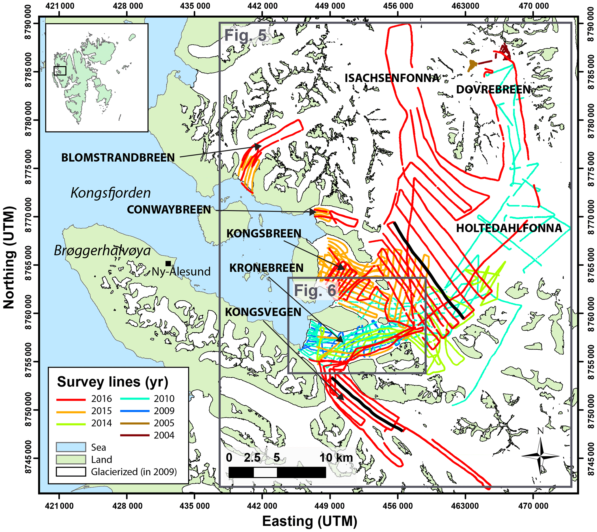
Figure 1 Radar survey lines collected between 2004 and 2016. Kongsfjorden, tidewater glaciers, icefields, the peninsula Brøggerhalvøya, and the research town Ny-Ålesund are marked in the map. The small inset map shows the location of Kongsfjorden in Svalbard. The blue areas are sea, green areas are land, and white areas are glacierized regions (in 2009). The black lines indicate the location of the profiles in Fig. 4 and the boxes show the coverage of Figs. 5 and 6. Grid projection is Universal Transverse Mercator Zone 33W.

Glacier front areas are important feeding areas for seabirds and marine mammals (Kovacs et al., 2011; Kovacs and Michel, 2011; Loeng et al., 2005; Lydersen et al., 2014). In summer, glacier meltwater flows on, in, and under the glacier towards the front. This meltwater is typically discharged below the seawater surface, often at the base of the calving front. The relatively low density of these fresh waters forces them to rise rapidly, entraining large volumes of ambient fjord water. These meltwater plumes can breach the surface, then flow outward towards the mouth of the fjord, further entraining subsurface water. In Svalbard, several bird species can be found in large numbers, up to thousands of individuals, at tidewater glacier fronts. The birds are often found in the so-called “brown zone”, the meltwater plume, which is ice-free and muddy due to upwelling suspended sediments and currents. These brown zones are also foraging hotspots for Svalbard's ringed seals and white whales (Lydersen et al., 2014). When the tidewater glaciers retreat so much that they become land-terminating, outflow into the fjord will only occur via surface drainage, just as with any un-glaciated fjord, with a cap of fresh river water flowing over the denser ocean water. This will lead to fewer nutrients and plankton being brought to the surface from the fjord bottom, which is likely to affect fjord ecosystems. Changes in freshwater flux from western Svalbard glaciers may also, in extreme climate warming scenarios, disturb deep-water production on the Svalbard shelf (Hagen et al., 2003). The amplified climatic warming at northern high latitudes (Serreze and Barry, 2011) makes Svalbard glaciers prime targets for understanding not only glacial dynamics but also the effects of ongoing climate change on glaciers, oceans, and ecosystems. To model future scenarios of fjord circulation and glacier dynamics, knowledge on the subglacial topography and bathymetry under the retreating glaciers is vital. Here, we present high-resolution (150 m gridded) digital elevation models (DEMs) of the subglacial topography, ice thickness, and elevation of five tidewater glaciers in Kongsfjorden, northwestern Spitsbergen, near Ny-Ålesund (78.9^∘ N, 12.4^∘ E).

2 Study area

Kongsfjorden is the southern branch of the Kongsfjorden–Krossfjorden system that merges towards the open sea, in a large submarine trough, Kongsfjordrenna, which channelled a fast-flowing ice stream during the last glacial maximum (Ingólfsson and Landvik, 2013; Ottesen et al., 2005). Kongsfjorden is ∼20 km long and between 4 and 10 km wide and covers an area of ∼200 km² and a water volume of ∼30 km³ (Ito and Kudoh, 1997). The maximum depth in the outer part of the fjord is 350 m and 100 m in the inner fjord. The mouth of the fjord lacks a well-defined sill and is therefore interconnected with neighbouring water masses on the West Spitsbergen Shelf, including Atlantic Water (Svendsen et al., 2002). Five tidewater glaciers terminate in Kongsfjorden (Fig. 1): Blomstrandbreen, Conwaybreen, Kongsbreen (with a north and south branch around Ossian Sarsfjellet), Kronebreen, and Kongsvegen. Kronebreen is among the fastest-flowing glaciers in Svalbard, with speeds up to ∼3 m d⁻¹ (Schellenberger et al., 2015). Upglacier from Kongsbreen and Kronebreen are two large icefields, Holtedahlfonna (named Dovrebreen in the upper part) and Isachsenfonna. In the following section, a short summary of the glacio-geomorphological setting of the study area is presented.

Glacio-geomorphological setting

The youngest deposits in Kongsfjorden are of Quaternary age and these landforms around Kongsfjorden are shaped by glacial activity (Ingólfsson and Landvik, 2013). Brøggerhalvøya and the areas to the north were probably completely ice-covered during the last Weichselian ice age. Compared to most other places in Svalbard, the Kongsfjorden area shows a more complete glacial sedimentary record dating back to before the last interglacial, the Eemian (Landvik et al., 2005). Together with Bellsund and Isfjorden, Kongsfjorden was one of the largest outlets for palaeo-ice streams in western Svalbard. The glaciers along the west coast of Svalbard had a complicated topographically controlled configuration during the Weichselian (Howe et al., 2003). The ice stream in Kongsfjordrenna was fed by ice draining through the deep fjord systems of Kongsfjorden and Krossfjorden, which drained a large section of the ice fields over northwestern Spitsbergen. Adjacent to the ice stream there were sharp boundaries to dynamically less active ice.

The glaciers started to retreat during the early Holocene and the region was likely largely ice-free until the neoglacial advance ∼4.5 thousand years ago. The bedrock has a relict subglacial, ice-scoured topography from the glacial re-advances of the Weichselian glaciation, with drumlins and glacial flutes common across the sea floor (Howe et al., 2003). Brøggerhalvøya shows four isostatically induced cycles of emergence out of the sea during the Weichselian glaciation (Miller et al., 1989), with beach ridges up to the marine limit at ∼80 m above sea level (a.s.l.). The current isostatic uplift rate is 8 mm y⁻¹ (Kierulf et al., 2009).

The bottom of inner Kongsfjorden has waveform morphology interpreted as moraines, partly originating from surges (Howe et al., 2003). Three glaciers are documented as surge type glaciers: Kronebreen–Kongsvegen surged around 1869 and 1897 (Bennett et al., 1999), Kongsvegen around 1948 (Liestøl, 1988; Woodward et al., 2002), and Blomstrandbreen, possibly between 1911 and 1928 (Burton et al., 2016), around 1960 (Hagen et al., 1993), and recently in 2010 (Mansell et al., 2012). Glacier surges lead to short-term reworking of sediments and deposition of sediment lobes containing massive glaciomarine muds with sedimentation accumulation rates up to 30 cm y⁻¹. Suspension settling from meltwater plumes and ice rafting are the dominant sedimentary processes, leading to the deposition of stratified glaciomarine muds with clasts from melting icebergs. The fjord topography has been smoothed by bottom currents.

3 Data and methods

We map the glacier beds with ice-penetrating radar (Dowdeswell and Evans, 2004). Our analysis builds on extensive radar campaigns conducted in the area from 2004 to 2016 (Fig. 1). Earlier campaigns (1988 to 2005) covered the upper parts of the glaciers, but the airborne radar failed to detect the bed in the lower reaches. This was caused by a too-high radar frequency (dictated by limitations on antenna size on an airplane) and too-high travel speed with respect to the data acquisition rate, as well as radar clutter from the rough surface, crevasses, and water within the glacier (Hagen and Sætrang, 1991). In recent years, radar surveys have successfully detected the bed in the lower parts of the glaciers using a lower frequency set-up mounted on a helicopter frame (Fig.  2). In the following sections, we describe the methods used to collect, process, and interpolate the radar data sets into the final products of gridded subglacial elevation and ice thickness. Surveys of crevassed glaciers from helicopters are less common (e.g. Blindow et al., 2012; Kennett et al., 1993; Langhammer et al., 2017; Rutishauser et al., 2016) than surveys from fixed-wing airplanes (e.g. Bamber et al., 2013; Fretwell et al., 2013; Morlighem et al., 2017). Therefore, we describe the set-up in detail.

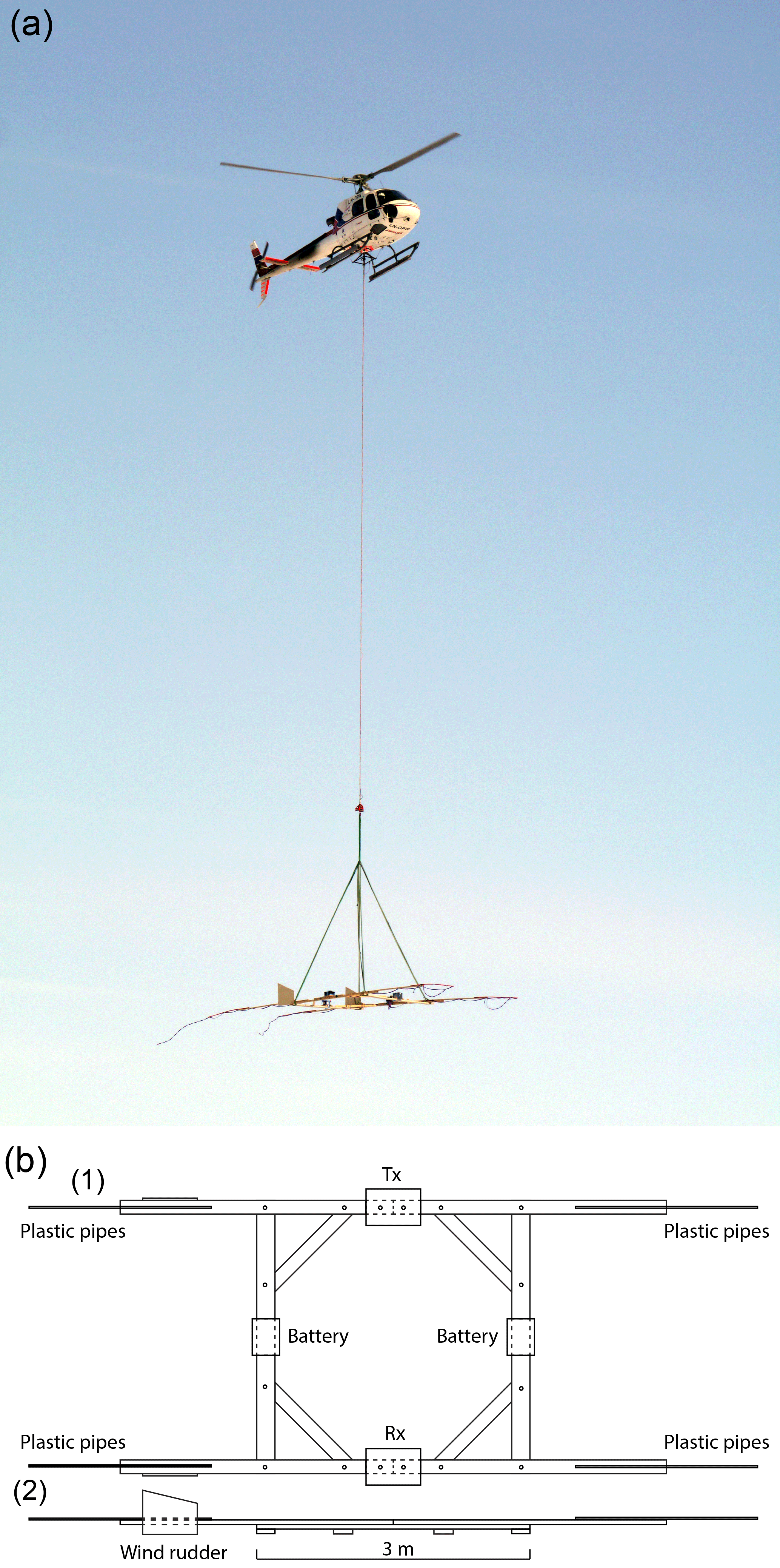
Figure 2 (a) Helicopter with radar frame. Photo: Nick Hulton. (b) Helicopter wooden frame (1) from above, with transmitter (Tx), receiver (Rx), two batteries and four plastic pipes for holding the antennas, and (2) from the side, with two fins on one side that function as wind rudders to prevent the frame from spinning. The antennas are connected to the Tx and Rx and fixed to the frame extending out on the plastic rods.

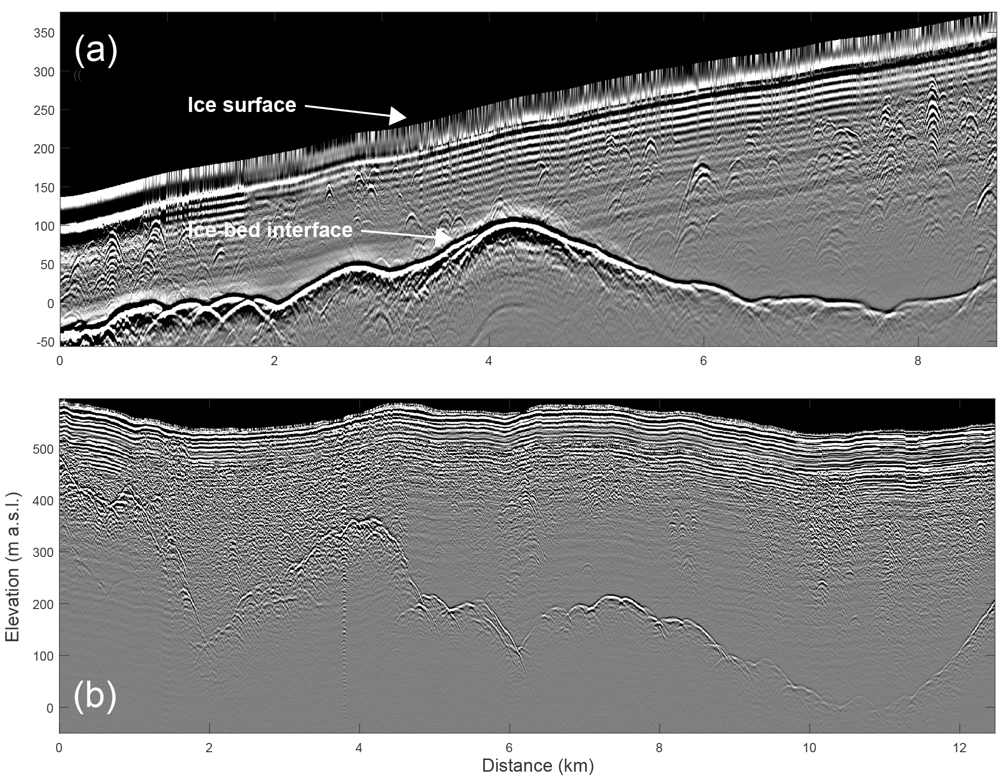
Figure 3 Examples of processed radar images collected on (a) Kongsvegen by snowmobile and (b) Holtedahlfonna by helicopter. Locations of the profiles are marked in Fig. 1 with black lines.

3.1 Radar systems and uncertainties

3.1.1 Radar data collected 2014 to 2016

During early spring (April to May) in 2014, 2015, and 2016 we collected ∼1300 km of common-offset radar profiles with an impulse radar system that was either suspended under a helicopter (for crevassed areas; Fig. 2a) or towed behind a snowmobile. The system is based on radar developed for surveying ice thickness on the Greenland ice sheet (Lindbäck et al., 2014). The radar system consisted of resistively loaded half-wavelength dipole antennas of 10 MHz centre frequency. We used a commercial off-the-shelf Kentech impulse transmitter with an average output power of 35 W and a pulse repetition frequency of 1 kHz. The trace acquisition was triggered by the direct wave pulse between transmitter and receiver. The 14-bit A/D converter sampled two channels at 125 MHz sampling frequency, with different sensitivity ranges. One channel was attenuated with 20 dB to record both the surface and the bed return.

Using the helicopter-based system, we surveyed the glaciers at a nominal speed of ∼40 km h⁻¹, along tracks separated by ∼0.5 to 1 km. By stacking 125 traces, a mean trace spacing of 4 m was achieved. We mounted the system on a 3×3 m wooden frame, with extended wooden arms and plastic rods for the antenna (Fig. 2b). The frame was suspended 20 m below the helicopter. The radar was controlled by wireless connection to a PC inside the helicopter. We used the ground-based system to survey the snowmobile-accessible Kongsvegen glacier. The system was mounted on two sleds and towed behind the snowmobile at a speed of ∼20 km h⁻¹. Stacking 125 traces resulted in a mean trace spacing of 2 m. We positioned the traces by using data from a code-phase global positioning system (GPS) receiver in 2014 and 2015 and a carrier-phase dual-frequency GPS receiver in 2016, mounted on the radar receiver box 1.5 m in front of the common mid-point along the travelled trajectory on the helicopter frame and 15 m from the common mid-point on the snowmobile. For the dual-frequency receiver we processed the data kinematically using the Canadian Spatial Reference System precise point positioning service (Natural Resources Canada, 2017).

We applied several corrections and filters to the radar data: (1) a Butterworth bandpass filter, with cut-off frequencies of 2 and 50 MHz, to remove unwanted frequency components in the data; (2) normal move-out correction to correct for antenna separation (including adjusted travel times for the trigger delay); (3) rubber-band correction to re-sample the data to a uniform trace spacing; and (4) two-dimensional frequency wave-number migration (Stolt, 1978) to collapse hyperbolic reflectors back to their original positions in the profile direction. On the high gain channel, we applied a spreading and exponential compensation (SEC) gain to amplify bed returns. The surface and bed returns were digitized semi-automatically with a cross-correlation picker (Irving et al., 2007) at the first break of the bed reflection. We calculated ice thickness from the picked travel times of the bed return using a constant radio-wave velocity of 169 m µs⁻¹ for ice. For the airborne profiles, we removed the travel times to the surface return using a constant radio-wave velocity of 300 µm s⁻¹ for air. We converted the GRS80 ellipsoidal heights to heights above sea level with a geoid model developed by the Norwegian Polar Institute, where the average geoid height is $\sim \mathrm{35}\pm \mathrm{0.5}$ m in the study area relative to the ellipsoid. Figure 3 shows examples of processed radar images.

3.1.2 Radar data collected 2004 to 2010

In addition to the data collected in this study, we used two additional data sets of unpublished radar data collected earlier by the Norwegian Polar Institute on (1) Dovrebreen in 2004 and 2005, and (2) Kronebreen and Holtedahlfonna in 2009 and 2010. We did not use additional data sets collected in Kongsvegen in 1988 (ice thickness; Hagen and Sætrang, 1991) and 1995 (subglacial elevation and ice thickness; Melvold and Hagen, 1998), because these data sets had large (>50 m) differences in subglacial elevation. This is because the data were collected over 20 years ago and possibly significant changes in glacier surface and subglacial sediment may hinder accurate estimates of subglacial elevations from these old ice-thickness data. Here follows a short summary of the two included data sets:

The Dovrebreen campaign. The data set consists of ∼ 22 km of radar profiles collected on the upper parts of Dovrebreen, during an ice coring campaign (Beaudon et al., 2013; Sjögren et al., 2007). The subglacial elevation and ice thickness were measured in April 2004 and 2005, with a 10 MHz centre frequency impulse radar. A single channel impulse radar based on a Narod transmitter (Narod and Clarke, 1994) and a 12-bit A/D converter in the receiver were used with restively loaded dipoles as antennas. The radar was operated at both 100 MHz sampling frequency and at 200, 300, and 500 MHz sampling frequency using repetitive sampling. The repetitive sampling gave a non-uniform sampling frequency in the scan, and the data had therefore been resampled to an equal time base between the samples with linear interpolation. An antenna separation of 20 m was used. The antennas were configured with the transmitter in the back and the receiver approximately 25 m behind a snowmobile. The profiles were positioned with a code-phase GPS receiver attached to the radar receiver and the position was recorded each second.

The Kronebreen and Holtedahlfonna campaign. The data consist of ∼340 km of radar profiles collected in 2009 to 2010, where both helicopter and snowmobiles were used. Data were collected with an impulse dipole radar comprising a Kentech pulser (average output power of 35 W), 10 MHz resistively loaded wire dipole antennas, and a 12-bit A/D converter. The helicopter and ground-based system was similar to the one previously described (see Sect. 3.1.1). The A/D converter sampled with two channels at 50 MHz sampling frequency. Five traces were stacked in flight, and further stacking was done during post-processing. Positioning was made with a code-phase GPS receiver attached to the radar receiver.

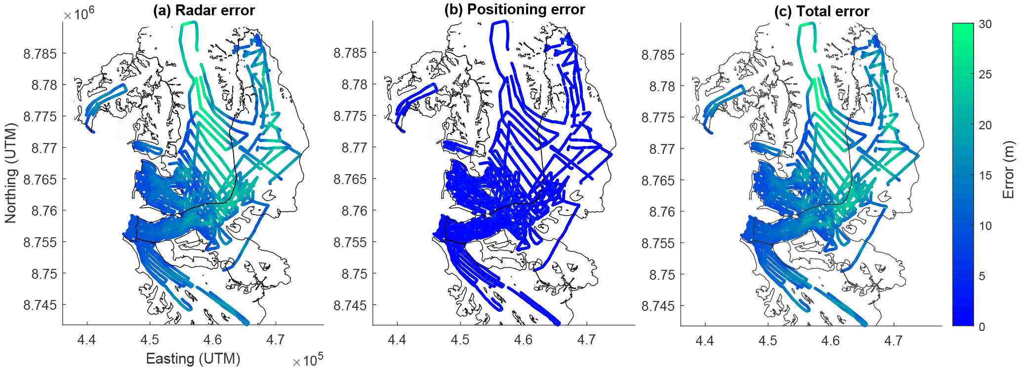
Figure 4 Errors in the subglacial elevation for each data point: (a) radar error consisting of the technical and theoretical capacity of the radar systems, (b) positioning error, and (c) the total error when combining radar and positioning errors. Grid projection is Universal Transverse Mercator Zone 33W.

3.1.3 Radar system errors and uncertainty

We used standard analytical error propagation methods (Lapazaran et al., 2016; Taylor, 1996) to calculate the error in subglacial elevation for each data point:

$$\begin{array}{}\text{(1)}& {\displaystyle }{\mathit{\epsilon }}_{\mathrm{bed}\mathrm{data}}=\sqrt{{\mathit{\epsilon }}_{\mathrm{radar}}^{\mathrm{2}}+{\mathit{\epsilon }}_{xy}^{\mathrm{2}}},\end{array}$$

where ε_radar was the error in the radar acquisition and ε_xywas the positioning error. The error in radar acquisition was calculated by the following:

$$\begin{array}{}\text{(2)}& {\displaystyle }{\mathit{\epsilon }}_{\mathrm{radar}}={\displaystyle \frac{\mathrm{1}}{\mathrm{2}}}\sqrt{v^{\mathrm{2}}\cdot {\mathit{\epsilon }}_t^{\mathrm{2}}+t^{\mathrm{2}}\cdot {\mathit{\epsilon }}_v^{\mathrm{2}}},\end{array}$$

where v was the radio-wave velocity used for time-to-depth conversation, t was the two-way-travel time of the radio wave and ε_t and ε_v were the errors in t and v respectively. We used a constant wave-propagation speed for the ground-based and airborne surveys (169 m µs⁻¹). Wave velocity can vary spatially, depending mostly on density. Profiles were collected in the ablation and accumulation zone with a snow and firn cover of up to 20 m thick in the upper parts of Dovrebreen (Beaudon et al., 2013; Woodward et al., 2003). We used a typical variation of 4 % of glacier ice density for the calculation of ε_v (Seligman, 1936). Variations in the wave velocity can also occur because of varying ice temperature and the presence of inhomogeneities and liquid water in the ice (Drewry, 1975). These effects are expected to have a small impact on the average velocity for the whole ice column, while water content in the ice can influence the velocity in a substantial way. In most parts of the study area the ice is cold (Beaudon et al., 2013; Woodward et al., 2003) and there are limited amounts of liquid water. We therefore neglect variations of velocity due to water content. The upper parts of Holtedahlfonna contain a firn aquifer (Christianson et al., 2015), but it comprises a small part of the total glacierized area, and is not accounted for. For ε_t we calculated the range resolution, which is the accuracy of the measurement of distance between the antenna and the bed and can be determined from the characteristics of the source pulse (i.e. bandwidth) and the digitization frequency. The range resolution for the data collected in this study was estimated at 8.5 m. We also included the vertical resolution, by taking the inverse of the radar frequency (Lapazaran et al., 2016). This results in values of ε_radar between 8.5 m (thin ice) and 30.5 m (thick ice) with a mean value of 14.3 m and standard deviation of 4.2 m (Fig. 4a). We calculated the positioning error ε_xy at each data point depending on the bed slope angle along the profile, following the method by Lapazaran et al. (2016). We assumed a helicopter-travel speed of 40 km h⁻¹, snowmobile-travel speed of 20 km h⁻¹, and T_GPS≤T_GPR (case a^′ in Appendix B of Lapazaran et al. 2016). This produced values of ε_xy between 0 (flat bed) and 76.0 m (steep bed $\sim \mathrm{90}{}^{\circ }$), with a mean value of 1.4 m and standard deviation of 2.1 m (Fig. 4b). The total error in subglacial elevation along the profiles (Eq. 2) varied between 8.5 and 78.0 m, with a mean of 14.5 m and standard deviation of 4.3 m (Fig. 4c).

To test the consistency between the data sets we also compared the crossover differences in the subglacial elevation estimates between different profiles and data sets. The data set collected in this study (2014 to 2016) had a median crossover misfit in subglacial elevation of 11.1 m with a standard deviation (σ) of 17.4 m based on 208 crossing points. The Dovrebreen campaign data set (2004 to 2005) had a median crossover misfit of 13.1 m (σ=12.7 m) based on 85 crossing points. The Kronebreen and Holtedahlfonna campaign data set (2009 to 2010) had a median crossover misfit of 3.9 m (σ=13.0 m) based on 136 crossing points. As the crossover analysis within the same data set does not capture systematic errors between the different data sets, we also did a comparison between the data sets. When we ran a crossover analysis between all the data sets the median misfit was 9.2 m (σ=15.7 m).

3.2 Surface and bathymetric elevation data

To obtain surface elevation for the study area that is most temporally consistent with the acquired helicopter thickness measurements, we used TanDEM-X monostatic radar images (Moreira et al., 2004) acquired on 20 December 2014. These images were processed by differential interferometry using Gamma Software (e.g. Neckel et al., 2013; Rankl and Braun, 2016) as precise orbital information is not publicly available. The monoscopic images were first co-registered to each other and to a previous baseline DEM derived from the TanDEM-X intermediate DEM (Wessel, 2016). After phase filtering, the differential phase was unwrapped using a minimum cost flow (MCF) algorithm and triangulation to provide elevation differences in metres between the intermediate DEM and that from the monoscopic images. Unwrapping was successful over the relatively flat terrain, with no apparent blunders even over steeper terrain. These differences were then added back to the TanDEM-X intermediate DEM to provide elevations from 20 December 2014 at a 12 m resolution. The obtained 2014 TanDEM-X elevations were for the underlying ice and ground surface as the X-band satellite radar wave can penetrate through the winter snowpack, providing a reflector from the ground and ice interface. On stable terrain surrounding the glaciers, the 2014 TanDEM-X DEM shows little bias, with a standard deviation of ∼4 m compared with the 2009 aerial-photogrammetric DEM from the Norwegian Polar Insitute (2014), which has a 5 m gridded resolution and a stated accuracy of ∼2 to 5 m. Elevation changes between 2009 and 2014 have mostly occurred close to the margins of the tidewater glaciers (<5 km), with up to 5 m of surface lowering (Cesar Deschemps, personal communication, 2017). This TanDEM-X DEM was merged with the NPI (2014) DEM to cover Blomstrandbreen, which is located outside of the TanDEM-X DEM, and downsampled to 150 m.

The offshore bathymetric DEM was compiled by the Norwegian Mapping Authority Hydrographic Service and is a publicly available data product (Kartverket, 2018). Data were acquired in 2000 with an EM 1002 multi-beam echo sounder. In 2007, 2010, and 2011 an EM 3002 multi-beam echo sounder was used. They derived the 50 m grid DEM in 2014 with the software QPS Fledermaus and CARIS HIPS/CARIS BathyDataBASE. The surface and bathymetric DEMs were point sampled and added to the subgrid of the radar data, described in detail below.

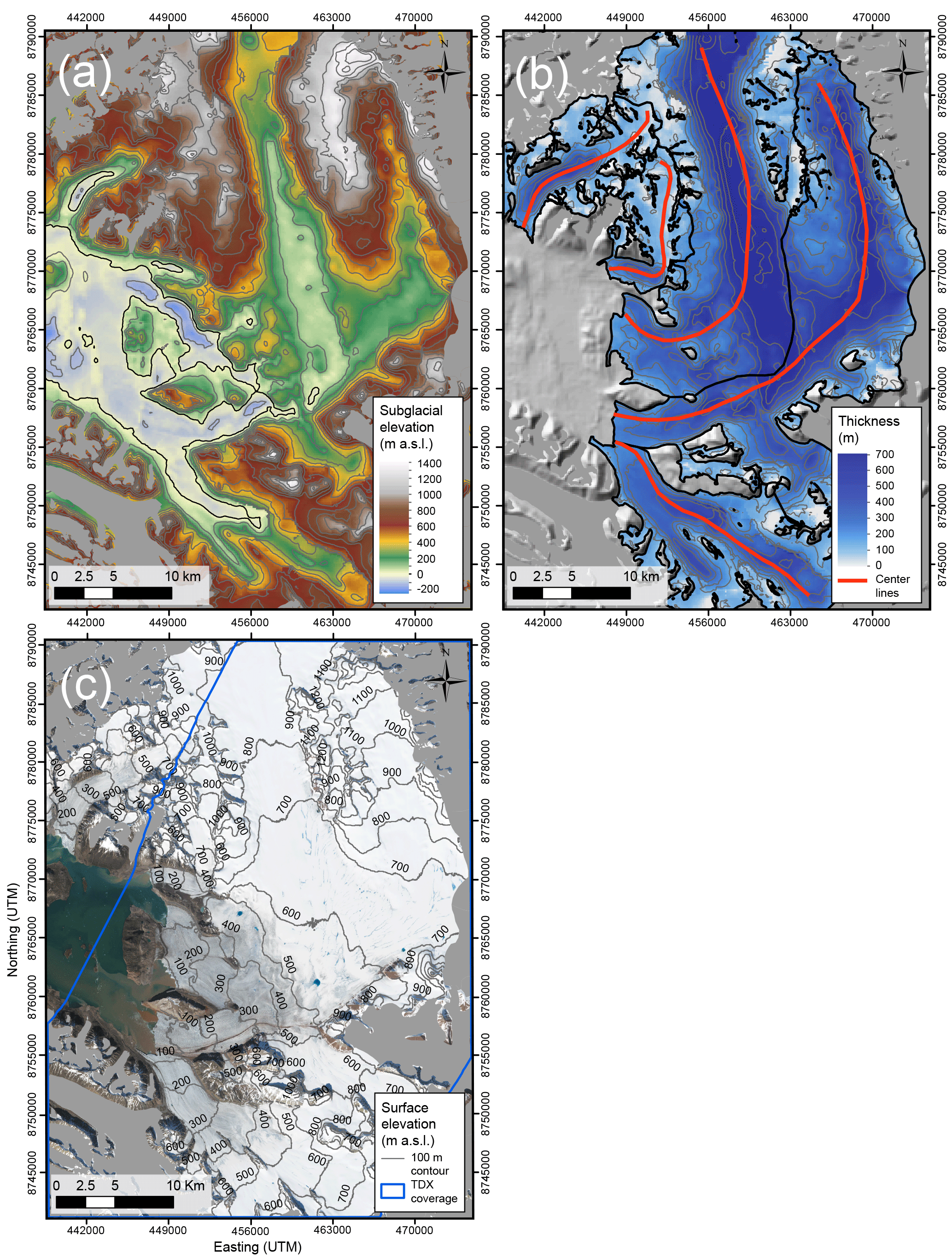
Figure 5 (a) Subglacial, bathymetric, and land elevation with 100 m elevation contours (grey lines). (b) Ice thickness in 2014 with 100 m elevation contours (grey lines) and glacier surface elevation catchments (black polygons). Hillshade image in the background from Fig. 5a. Statistics for each glacier are specified in Table 1. (c) Surface elevation in 100 m contours showing the extent of the TANDEM-X (TDX) DEM (blue polygon). Background image is Sentinel-2 satellite image taken on 10 July 2016 (Copernicus, 2016). Grey areas in all figures are glaciers not covered in the study. Grid projection is Universal Transverse Mercator Zone 33W.

3.3 Assimilation of the data sets

We combined the different data sets of subglacial, land, and bathymetry elevation to a final gridded elevation DEM. The measuring interval for the radar data sets are dense along the profiles, with a data point spacing of ∼5 m, compared with ∼50 to 1000 m spacing between individual profiles. As this non-uniform spacing is not optimal for gridding algorithms, we sub-gridded data sets into a 100 m pseudo-grid to reduce the data density along individual profiles. The subgrid was produced by calculating the median values for the points that fell within the distance of half the grid cell. To prevent steps at the borders between the subglacial and proglacial DEMs we point-sampled the land-topography and bathymetric DEMs outside the glacierized areas and added these points to the subgrid. We used a universal kriging algorithm (e.g. Isaaks and Srivastava, 1989) for the interpolation. To calculate glacier ice thickness in 2014, we subtracted the subglacial DEM from the combined TanDEM-X DEM and NPI DEM. We did this instead of using ice thickness measurement for each radio echo-sounding data set, to make the subglacial DEM more consistent over the area, as the ice thickness has changed since the first data were collected in 2004.

The subglacial DEM agrees well with a borehole study in Kronebreen in 2014 (How et al., 2017), with a measured subglacial elevation of −93 m a.s.l., where the gridded DEM predicts a depth of 90 m. To assess the error in interpolation we cross-validated the gridded data, which is a common validation technique to see how well an interpolated model is influenced by the observed data. By removing one observation from the data set, the remaining data were used to interpolate a value for the removed observation. This process was continued for 1000 random observations in the data, where the error is the residual between the observed and the interpolated value (Isaaks and Srivastava, 1989). The standard deviation of the residuals was estimated to be 18 m, and increases with distance from the profiles. To summarize, the total accuracy of the gridded subglacial elevation depends on: (1) the technical and theoretical capability of the radar systems, (2) positioning errors, and (3) interpolation errors. By assessing all these potential sources of error, we estimate the maximum vertical root-mean-squared uncertainty in the final subglacial and ice thickness DEMs to be approximately ±24 m.

4 Results

We present DEMs of subglacial topography (Fig. 5a), ice thickness (Fig. 5b), and ice surface elevation (Fig. 5c) of a 1100 km² area of Svalbard on a 150 m grid. The DEMs cover the tidewater glaciers Blomstrandbreen, Conwaybreen, Kongsbreen, Kronebreen, and Kongsvegen and are merged with bathymetric and land DEMs for the non-glaciated areas. The large-scale subglacial topography of the study area is characterized by a series of troughs and highs. The minimum subglacial elevation is −180 m a.s.l., the maximum subglacial elevation is 1400 m a.s.l., and the maximum ice thickness is 740 m. We estimate the maximum vertical root-mean-squared uncertainty in the subglacial and ice thickness DEMs to be approximately ±24 m. The statistics for each glacier are summarized in Table 1. For Kronebreen, which has a dense data coverage (Fig. 1), we also present a 50 m gridded subglacial DEM (Fig. 6). In the following paragraphs, we describe the main troughs and highs in the subglacial topography. Overdeepenings in Blomstrandbreen and Conwaybreen (−110 and −60 m a.s.l., respectively; Figs. 5a, 7a, and b) lie behind sills at the glacier front, which limit the extension of the fjord further upglacier; both overdeepenings will therefore likely be either filled with sediments or freshwater, as the glaciers retreat. Further south, Kongsbreen consists of two tributary outlets around the Ossian Sarsfjellet. Kongsbreen North has a deep trough beneath it with a minimum elevation of −180 m a.s.l (Figs. 5a and 7c). The continuation of the fjord (i.e. elevation beneath current sea level) extends 11 km inland from the current front to north of the nunatak Steindolpen, upglacier from Collethøgda. The fjord may possibly connect with Kronebreen in a 500 m wide embayment, with only 10 m deep waters. Kongsbreen South has a sill at its front, with a minimum elevation of 8 m a.s.l., preventing the embayment in front of the glacier connecting to Kongsbreen North.

Table 1 Statistics for each glacier with subglacial elevation and ice thickness.

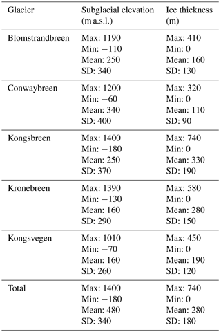
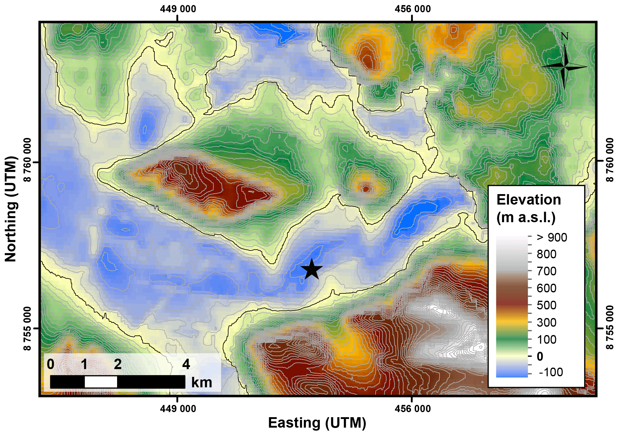
Figure 6 Subglacial, bathymetric, and land elevation of Kronebreen at 50 m gridded resolution with 20 m elevation contours. Location of the borehole study is marked with a black star (How et al., 2017). Grid projection is Universal Transverse Mercator Zone 33W.

Kronebreen, the fastest flowing glacier in the fjord (Schellenberger et al., 2015), has a trough beneath it with a minimum elevation of −130 m a.s.l (Figs. 5a, 6 and 7d). The trough continues 10 km inland, where it ends at a 350 m wide and 2 km long embayment with 20 m shallow waters. Upglacier from the embayment there is a steep sill, with a minimum elevation of 130 m a.s.l., which can also be seen at the glacier surface (Fig. 7d), where there is a steep and heavily crevassed ice fall. Further inland, the ice thickens again and there is a small overdeepening with a minimum subglacial elevation of −30 m a.s.l. The high-resolution subglacial DEM of Kronebreen has so far been used in studies of basal sliding, subglacial hydrology, and calving (How et al., 2017; Vallot et al., 2017, 2018).

The subglacial topography beneath Isachsenfonna consists of a 3 km wide flat valley with a minimum subglacial elevation of 40 m a.s.l (Figs. 5a and 7c). Holtedahlfonna has a 2 km wide valley with higher subglacial elevations, with a minimum elevation of 120 m a.s.l, and gradually higher elevations up on Dovrebreen (Figs. 5a and 7d). Finally, Kongsvegen, flowing in from the southeast towards Kronebreen, has a trough beneath it with a minimum subglacial elevation of −70 m a.s.l., which continues 9 km inland until just north of the nunatak Vorehaugen (Figs. 5a and 7e).

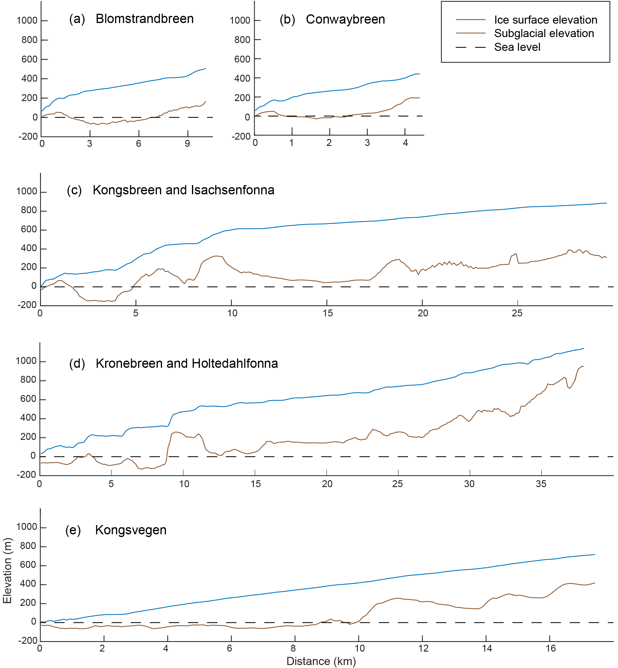
Figure 7 Glacier surface elevation in 2014 (blue line) and subglacial elevation (brown line) along the glacier ice flow centre lines (Fig. 5b) of (a) Blomstrandbreen, (b) Conwaybreen, (c) Kongsbreen and Isachsenfonna, (d) Kronebreen and Holtedahlfonna, and (e) Kongsvegen. Dashed black line is present-day sea level. Distance is measured from the present-day glacier front. Notice that the x axis scale varies between the plots.

5 Data availability

The compiled data sets of ground-based and airborne radar surveys are freely available at the Norwegian Polar Data Centre (https://doi.org/10.21334/npolar.2017.702ca4a7, Lindbäck et al., 2018). The data set will be updated when the quality of the data is improved or if new data sets become available.

6 Summary

Tidewater glaciers have a major influence on circulation in the water bodies in which they sit, particularly in constricted bays or fjords. In this study, we produced subglacial topography and ice thickness DEMs of five tidewater glaciers in Kongsfjorden on a 150 m grid. We also produced a 50 m gridded resolution DEM for Kronebreen, where the data coverage is dense. The subglacial elevation and ice thickness data consist of ∼1700 km common-offset radar profiles collected in 2004 to 2016 with an impulse radar system that was either suspended under a helicopter (for crevassed areas) or towed behind a snowmobile. We combined the data sets of subglacial elevation with land elevation and bathymetry elevation DEMs to a final gridded DEM. The large-scale subglacial topography of the study area is characterized by a series of troughs and highs, where the glaciers Kongsbreen, Kronebreen, and Kongsvegen have the potential to retreat by ∼10 km before they become land-terminating. The compiled data set covers one of the most studied regions in Svalbard and is valuable for future studies of glacier dynamics, geology, hydrology, and fjord circulation.