Estimating the thickness of unconsolidated coastal aquifers along the global coastline

Knowledge of aquifer thickness is crucial for setting up numerical groundwater flow models to support groundwater resource management and control. Fresh groundwater reserves in coastal aquifers are particularly under threat of salinization and depletion as a result of climate change, sea-level rise, and excessive groundwater withdrawal under urbanization. To correctly assess the possible impacts of these pressures we need better information about subsurface conditions in coastal zones. Here, we propose a method that combines available global datasets to estimate, along the global coastline, the aquifer thickness in areas formed by unconsolidated sediments. To validate our final estimation results, we collected both borehole and literature data. Additionally, we performed a numerical modelling study to evaluate the effects of varying aquifer thickness and geological complexity on simulated saltwater intrusion. The results show that our aquifer thickness estimates can indeed be used for regional-scale groundwater flow modelling but that for local assessments additional geological information should be included. The final dataset has been made publicly available (https://doi.pangaea.de/10.1594/PANGAEA.880771).

1 Introduction

Coastal aquifers provide fresh groundwater for more than 2 billion people worldwide (Ferguson and Gleeson, 2012). Multiple local and regional studies have shown that these fresh groundwater resources are threatened not only by natural disasters such as storm surges and tsunamis (Cardenas et al., 2015), but also increasingly by climate-induced sea-level rise (Carretero et al., 2013; Rasmussen et al., 2013; Sefelnasr and Sherif, 2014) and urbanization that lead to coastal aquifer over-exploitation combined with reduced groundwater recharge (Custodio, 2002).

Table 1 Statistics for individual GLIM classes in the coastal ribbon (200 km and less from the coastline). The population numbers are based on the 2015 global population count (CIESIN, 2017).

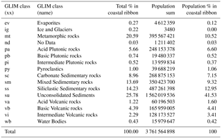
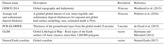
Table 2 Summary of the global datasets used for aquifer thickness estimation.

Comparing coastal aquifer vulnerabilities worldwide in a consistent manner requires a global-scale study (Döll, 2009). However, many necessary input datasets, both physical and societal, are only available on regional or local scales and can therefore only be used in coastal aquifer vulnerability investigations on a regional scale. Notable work on global coastal aquifer vulnerability are studies by Ranjan et al. (2009) and Michael et al. (2013) looking at coastal aquifer vulnerability to seawater intrusion and by Nicholls and Cazenave (2010) taking social–economic factors into account. Related observation-based studies are performed by van Weert et al. (2008) on global saline groundwater occurrence assessment and by Post et al. (2013) on the existence of offshore fresh or brackish groundwater. Lacking global information, the few global studies that attempted a modelling approach (i.e. Ranjan et al., 2009, and Michael et al., 2013) used globally or regionally homogenous hydraulic parameters, including aquifer thickness. Indeed, recent reviews concluded that most of the past modelling studies until the present day (on both local and global scales) considered a homogeneous aquifer system (Werner et al., 2013; Ketabchi et al., 2016). This pinpoints that there is still a large gap in our knowledge about coastal aquifer hydrogeological settings in many parts of the world. Since the local and regional hydrogeological conditions largely determine the coastal aquifer vulnerability to sea-level rise (Michael et al., 2013) and groundwater pumping (Ferguson and Gleeson, 2012), it is important to improve our insight into the local and regional coastal aquifer hydrogeology worldwide.

The goal of this study is to estimate the unconsolidated aquifer system thickness along the global coastline. This constitutes a first step towards a more complete hydrogeological characterization of coastal aquifers. Our focus is limited to aquifer systems formed by unconsolidated sediments (Table 1) that constitute around 25 % of the coastal ribbon (200 km far or less from the coastline) based on the GLIM (Global lithological map) dataset (Hartmann and Moosdorf, 2012). In contrast, more than 36 % is shaped by different types of sedimentary rocks where aquifers can also be expected. These sedimentary rock formations most probably form the coastal aquifer systems that are missed in this study. However, more than 40 % of people living in the coastal ribbon (CIESIN, 2017) are located on top of unconsolidated sediment aquifer systems (Table 1), while less than 30 % live in areas with sedimentary rock aquifers. This means that there is potentially more pressure on freshwater availability in areas with unconsolidated sediment aquifer systems.

To be globally applicable and comparable, our method of aquifer thickness estimation makes use of already available open-source global datasets (see Table 2). These datasets contain information on elevation, surficial lithology, regolith thickness and overall sedimentary thickness. What motivated this study is that none of the globally available thickness datasets are individually suited to representing coastal aquifer thickness. Two of these datasets only provide estimated regolith (surficial sediment layer) or soil thickness (Pelletier et al., 2016; Shangguan et al., 2017). The soil or regolith layer is only part of the aquifer system formed by unconsolidated sediments and therefore unfit to use in building a hydrogeological model representing the flow in the whole aquifer system. Conversely, the other two datasets (Whittaker et al., 2013; de Graaf et al., 2015) estimate the total porous media thickness without making a distinction between unconsolidated and consolidated sediments (rocks), and therefore tend to overestimate the unconsolidated aquifer system thickness.

The resulting dataset consists of 26 968 cross sections perpendicular to the global coastline with unconsolidated aquifer thickness estimated along each cross section. Additionally, the uncertainty ranges in aquifer thicknesses are provided for each cross section. In order to illustrate how to use the new dataset in a regional groundwater modelling setting, we will show the results of variable-density groundwater flow and coupled salt transport models for three distinctly different coastal cross sections. We also show the sensitivity of modelling results to varying the aquifer thickness and geological complexity.

2 Materials and methods

2.1 Coastal aquifer unconsolidated sediment thickness estimation

We collected state-of-the-art open-source global datasets (Table 2) that provide information on topography and bathymetry (Weatherall et al., 2015), regolith thickness estimation (Pelletier et al., 2016), global-scale aquifer thickness estimated by de Graaf et al. (2015), lithology (Hartmann and Moosdorf, 2012) and coastline position (Natural Earth, 2017). The core of our aquifer thickness estimation (ATE) method is to combine topographical and lithological information. This enables us to find the topographical slope of outcropping bedrock formations and to determine the coastal plain extent. The latter is defined by a low topographical slope (Weatherall et al., 2015), a lithology consisting of unconsolidated sediments (Hartmann and Moosdorf, 2012) and a regolith thickness thicker than 50 m (Pelletier et al., 2016). This is the first study that directly combines lithology and topographic information to estimate the coastal unconsolidated sediment aquifer systems thickness at global scale.

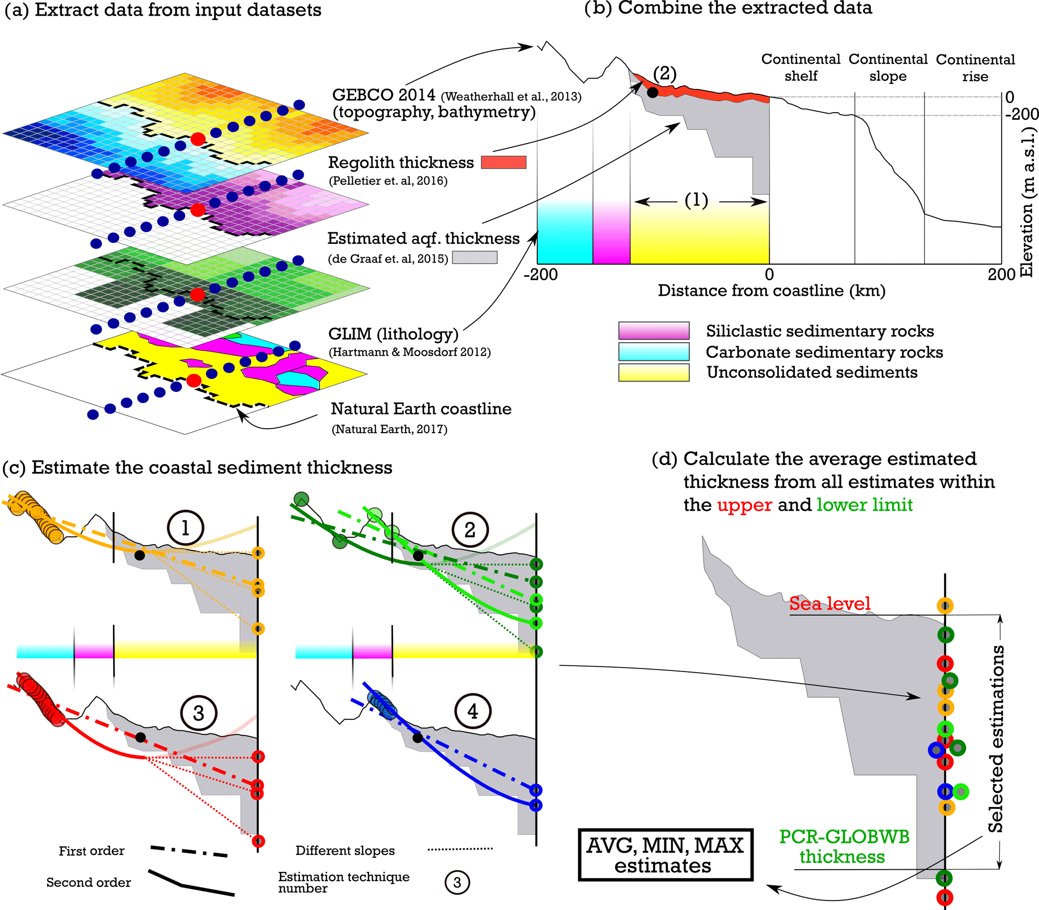
Figure 1 Schematization of the ATE method using available open-source global datasets. (a) Combining input datasets and extracting the values at cross-section points along a perpendicular cross section to the coastline running through a coastal point (red dot), only a few are schematized in the figure (in reality 800 per cross section). (b) Determine the extent of the coastal plain (1) and position of the anchor point (2). Extent of the cross section is set to 200 km landward and offshore; (c) the estimation is performed via topographical points selected based on the coastal plain extent, the position of the anchor points and the lithological classes from the GLIM dataset. The second-order estimation line is not used for estimation in case its minimum is reached before the coastline (transparent). (d) Final step of calculating the average, minimum and maximum estimated values.

Given the large variety of coastal environments, ranging from steep cliffs to extensive deltaic flat areas, it is important to develop a robust method that distinguishes between these different coastal types and also takes into account variations of inland bedrock formations. To achieve this, the coastal zones are represented as perpendicular cross sections to the coastline and are placed equidistantly (5 km) along the coastline. The intersections between the cross sections and the coastline are called coastal points. Along the cross section, a set of equidistant points (0.5 km) is positioned (cross-section points) and marks the locations where values from the datasets listed above are extracted (Fig. 1a). The cross sections span 200 km both inland and offshore from the coastal point to capture the bathymetrical and topographical profile. This distance was chosen to safely cover the necessary stretch both landward and offshore for groundwater flow and coupled salt transport modelling. Recent studies dealing with the latter set the landward boundary less than 200 km from the coastline even in deltaic areas (Delsman et al., 2014; Larsen et al., 2017; Nofal et al., 2016). Similarly, previous studies showed that submarine groundwater discharge can occur more than 100 km offshore (Kooi and Groen, 2001; Post et al., 2013).

Figure 1b shows an example of a cross section running through a coastal point. All the necessary values from the individual datasets are aggregated and used to determine the coastal plain extent and the anchor point position. The inland boundary point of the coastal plain is defined as a cross-section point that has a lithological class different than a water body (to take into account e.g. lagoons and bays) or unconsolidated sediments based on the GLIM dataset. Hartmann and Moosdorf (2012) state that uncertainty in the GLIM dataset is still significant based on the amount of mixed sediment class (∼15 % of the world area), so it is likely that some unconsolidated sediment coastal areas have been missed in our study.

Figure 2 Histogram of coastal plain extents and anchor point distance to coastline values.

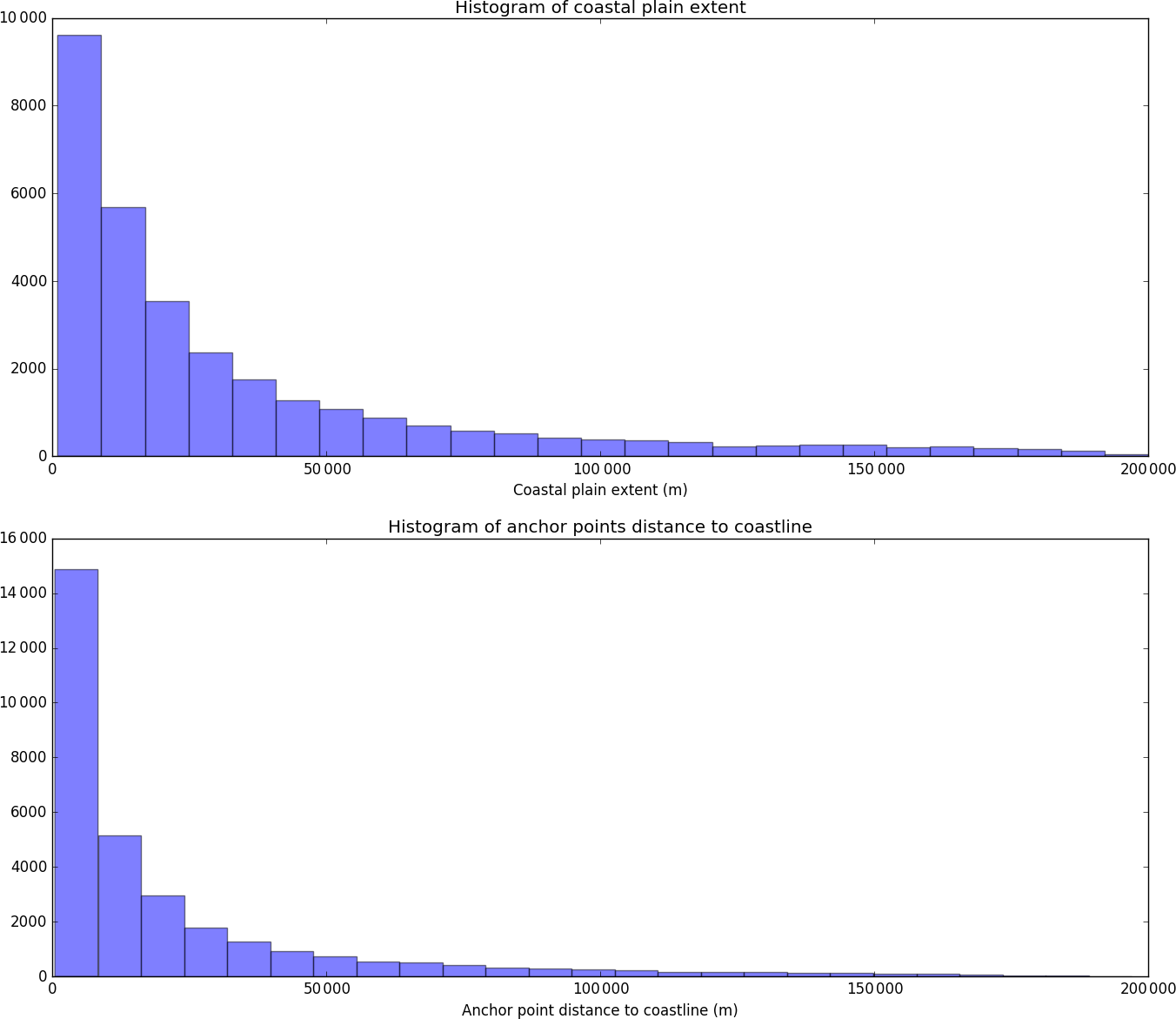
Once the coastal plain extent is known, the next step is to define the anchor point using the regolith thickness dataset (Pelletier et al., 2016). Taking note of the fact that the Pelletier et al. (2016) dataset generally has increasing thickness values towards the coast in case of unconsolidated sediments and that a thickness larger than 50 m is not mapped, we define the anchor point as the last cross-section point (moving from land to coast) with soil and sedimentary deposit thickness smaller than 50 m. Pelletier et al. (2016) state that areas with low relief, such as coastal plains, generally have a thicker sedimentary layer (>50 m) than hillslopes, so the transition zone between these two relief types is modelled with acceptable accuracy on global scale. The anchor point represents the last point where soil and sedimentary deposit thickness is known and is located below ground at the indicated depth by this dataset. A histogram of anchor point distances to coastline and of total coastal plain extent values is shown in Fig. 2. The ATE is then performed for all cross-section points located between the anchor point and the coastline.

Due to a large variety in the coastal plain extent, topography and geological diversity of the coastal cross sections worldwide, four different estimation techniques are proposed to increase the overall estimation method robustness. The differences between these techniques are in the topographical points' selection; these points are used to simulate the bedrock slope (Fig. 1c). The anchor point is added to the set of topographical points in every estimation technique.

The first technique selects all cross-section point elevation values of the first peak located prior to the coastal plain, regardless of lithological class. The second technique selects all the cross-section point elevation values of the highest peak located in a bedrock formation (any other class than unconsolidated sediments). The third selection technique consists of selecting all cross-section point elevations located between the coastal plain end and the bedrock formation end. The last technique selects only the local minimum and maximum points of every peak located behind the coastal plain. This diversity in selecting cross-section points based on lithological and topographical information combinations allows for a more robust method that is fit for various coastal environments.

For each selection technique described above, a first- and second-order curve fitting is performed to simulate the bedrock formation slope (Fig. 1c). If the minimum point of the second-order curve is situated before the coastline, we use three different linear function types to extend the bedrock slope simulation and estimate the sediment thickness by extending it beyond the coastline. All three lines start at the minimum point of the second-order estimation and run through the coastline. The first line is a constant horizontal line, the second simulates the average continental shelf slope (defined as shallower than −200 m b.s.l.) and the last line simulates the average slope of the whole 200 km cross-section offshore segment.

The global-scale aquifer thickness estimated by de Graaf et al. (2015) is chosen as the lower boundary since it tends to overestimate the coastal aquifer thickness because its underlying method is more fit for the inland areas and uses river networks and basins as a basis for thickness estimates (de Graaf et al., 2015). Finally, all the points are used to estimate the mean, minimum and maximum aquifer thicknesses at the coastline and the mean coastal profile for the unconsolidated sediment extent. The dataset that is stored contains per coastal cross section the mean profile as well as the maximum and minimum depth and the depth at the coastline standard deviation. For each coastal cross section, the anchor point position and depth are also included.

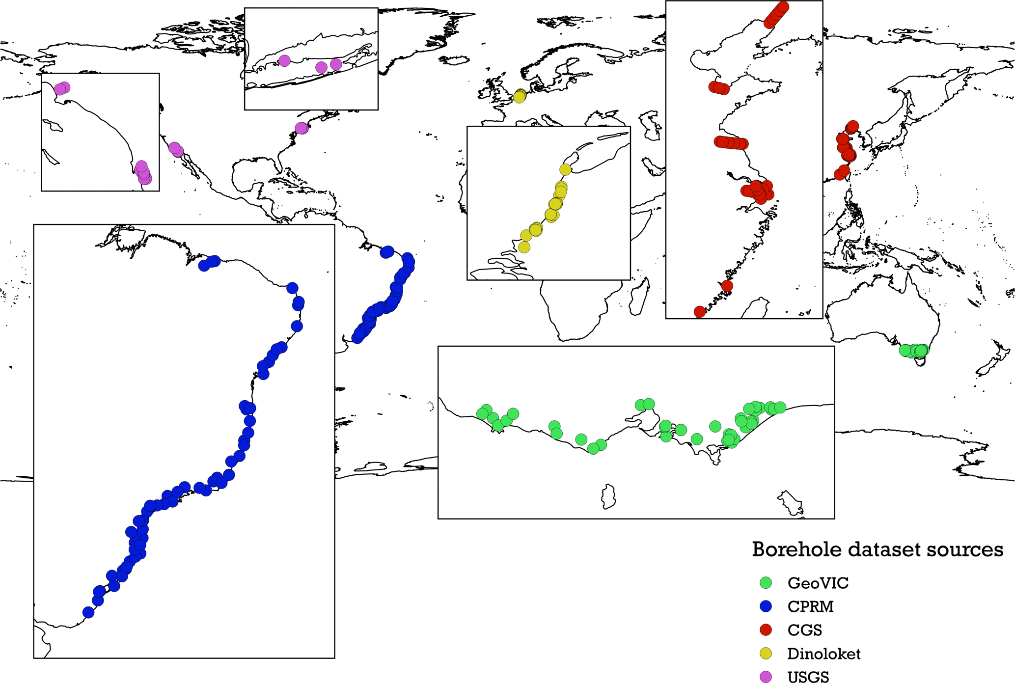
Figure 3 Location of the borehole data used as a validation dataset; sources are listed in Table S3. The borehole information in Brazil and Australia was manually digitized, while the subsurface information in China was gathered by interpreting the cross section provided in the hydrogeological maps.

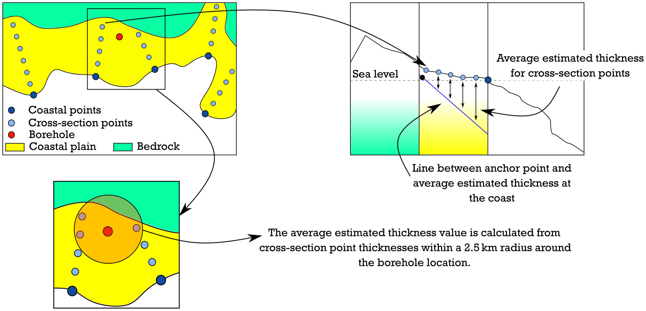
Figure 4 Schematization of the borehole validation process. A set of points lying within a given distance is selected for each borehole and their estimated sediment thickness is averaged. The final comparison between these average values and measured values from the boreholes is shown in Fig. 3 in the main article.

2.2 Validation methods

Two different validation approaches are applied to test the fit of our estimated aquifer thicknesses with measured values. First, the results are compared with information from available open-source geological borehole datasets. The second validation method consists of comparing the average estimated aquifer thickness with measured values gathered via a literature review.

A dataset incorporating 168 geological borehole descriptions was collected and sorted out from open-source datasets and web services, mostly located in the Netherlands, the USA, Brazil and Australia. After digitizing the borehole reports, we translated the geological information into overall unconsolidated sediment thickness to compare it to our final thickness estimates. This means that all the unconsolidated sediment types such as sand, clay or silt were merged into the same stratigraphic unit and their overall thickness is taken as the final sediment thickness. Figure 3 shows the collected borehole location, and the data sources are presented in Table S1 in the Supplement. Since some boreholes are not located in direct proximity to the coastline, we chose to extrapolate the estimated sediment thickness by calculating the estimated sediment thickness for each cross-section point. This was done by creating a line between the anchor point depth and the estimated sediment depth at the coastline (Fig. 4). Next, the average cross-section point thickness in a circle with radius of 2.5 km around the borehole is compared to the thickness in the borehole.

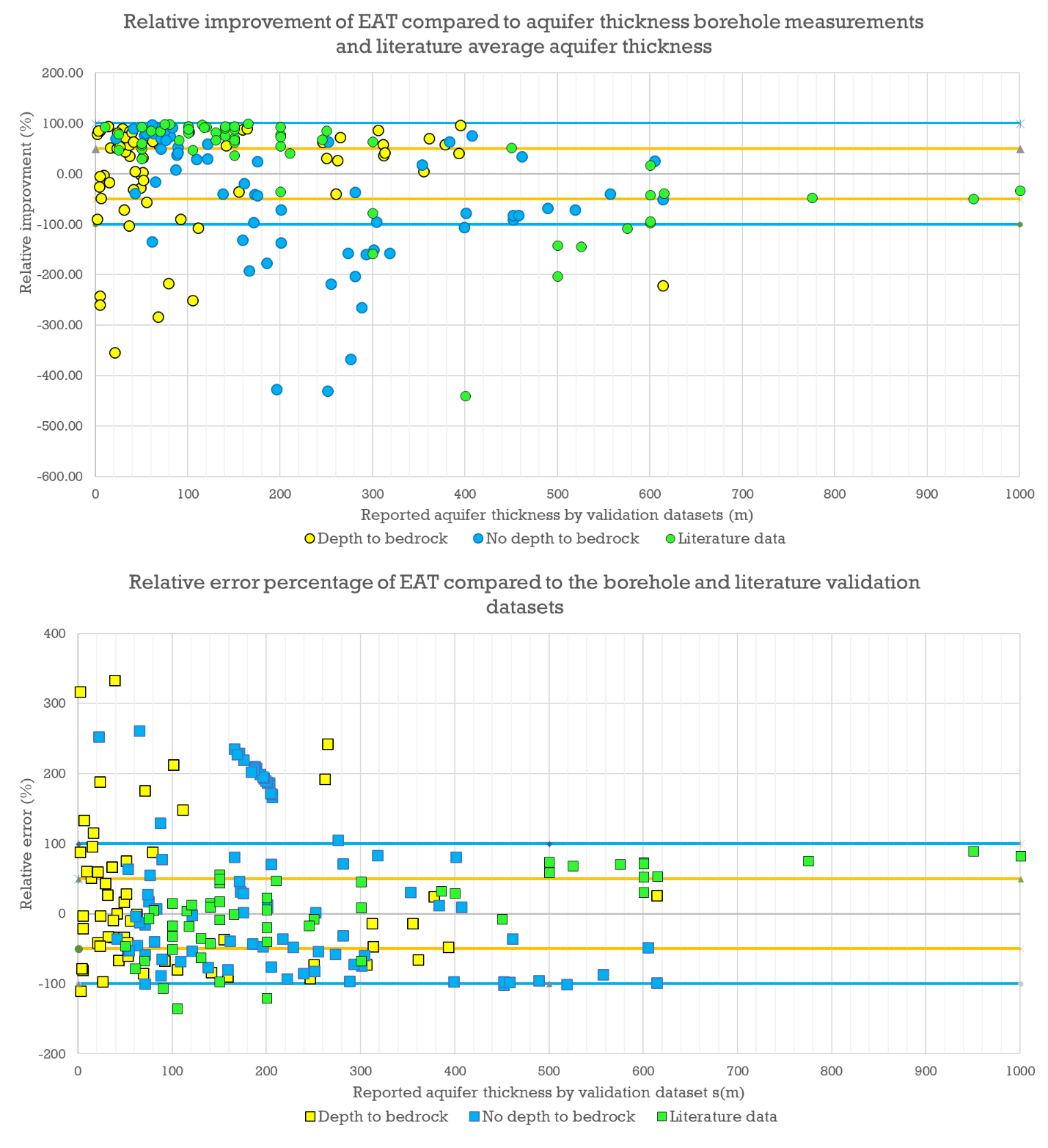
The final literature validation set is composed of maximum, minimum and/or average aquifer thickness values (unconsolidated sediment) for 64 coastal areas worldwide. However, not all the literature sources provide the average unconsolidated sediment thickness. In the cases where it does not, it is calculated as half the maximum indicated thickness in case only the maximum value is provided. If both maximum and minimum thicknesses are given, the average thickness is set to be halfway between these two values. The table with literature source references and the sediment thickness values provided by these sources are listed in Tables S2 and S3. The final estimated average sediment thickness values were compared with the literature dataset and evaluated based on the relative error and relative improvement compared to the overall average thickness value from all literature sources. The relative error is based on the following equation:

$$\begin{array}{}\text{(1)}& {\displaystyle }\text{RE}={\displaystyle \frac{Z_{\mathrm{est}}-Z_{\mathrm{lit}}}{Z_{\mathrm{lit}}}},\end{array}$$

where Z_est is the ATE by our method and Z_lit is the average thickness given by the literature. The RE can be either positive or negative, which implies that the ATE over- or under-estimates the aquifer thickness respectively (compared to values indicated by the literature). The percentage relative error is calculated as

$$\begin{array}{}\text{(2)}& {\displaystyle }\text{PRE}=\text{RE}\cdot \mathrm{100}.\end{array}$$

The average global aquifer thickness value based on all literature sources was calculated using the equation below:

$$\begin{array}{}\text{(3)}& {\displaystyle }{Z}_{{\mathrm{lit}}_{\mathrm{avg}}}={\displaystyle \frac{\mathrm{1}}{N}}{\sum }_{i=\mathrm{1}}^n{Z}_i,\end{array}$$

where $Z_{{\mathrm{lit}}_{\mathrm{avg}}}$ is the overall average value of all literature values Z_i.

The mean absolute error was then calculated for both the overall average value and the estimated average thickness values suggested by our method; see the equations below:

$$\begin{array}{}\text{(4)}& {\displaystyle }& {\displaystyle }{\text{MAE}}_{\mathrm{lit}}={\displaystyle \frac{\mathrm{1}}{N}}{\sum }_{i=\mathrm{1}}^n\mathrm{|}{Z}_{{\mathrm{lit}}_{\mathrm{avg}}}-Z_i\mathrm{|},\text{(5)}& {\displaystyle }& {\displaystyle }{\text{MAE}}_{\mathrm{est}}={\displaystyle \frac{\mathrm{1}}{N}}{\sum }_{i=\mathrm{1}}^n\left|Z_{\mathrm{est}}-Z_i\right|.\end{array}$$

Subsequently, the relative improvement rate and percentage relative improvement are calculated as follows:

$$\begin{array}{}\text{(6)}& {\displaystyle }& {\displaystyle }\text{RI}={\displaystyle \frac{{\text{MAE}}_{\mathrm{lit}}-{\text{MAE}}_{\mathrm{est}}}{{\text{MAE}}_{\mathrm{lit}}}},\text{(7)}& {\displaystyle }& {\displaystyle }\text{PRI}=\text{RI}\cdot \mathrm{100}.\end{array}$$

The same validation criteria are calculated using the borehole data.

2.3 Groundwater flow and salt transport modelling

The main motivation behind building numerical models simulating the groundwater flow and salt transport as part of this study is to examine the effects of varying aquifer thickness and its geological complexity (absence or presence of low permeable aquitard layers) on simulated saltwater intrusion. Better understanding of these sensitivities will help create improved large-scale hydrogeological models in coastal areas, which in turn will lead to more accurate present and future fresh groundwater volume predictions. To achieve that, a set of variable-density groundwater flow models with varying aquifer thickness and geological complexity (heterogeneous versus homogeneous systems) is created. To evaluate the sensitivity of saltwater intrusion to aquifer thickness and geological complexity, we compare, at a fixed time, the salinity profiles of all simulations as well as the freshwater cell percentage in the coastal zone.

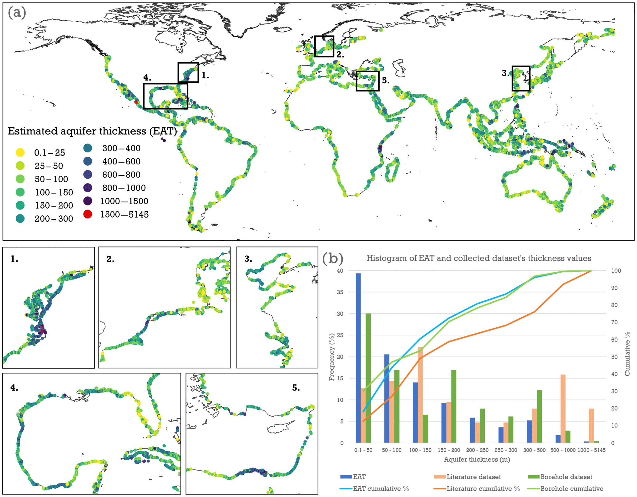
Figure 5 (a) Global map of EAT at the coastline and zoomed areas (1–5) showing regional variations of estimated thickness in various coastal zones around the world. The coastal points are magnified, giving the impression that more than the stated 20 % of the global coastline is covered, which is not the case (see the plain black line). (b) Histogram of EAT values with cumulative frequency in %.

The models with different parameter settings were set up for three cross sections located in Italy in the Versilia plain (Pranzini, 2002), the coast of Virginia in the USA (Trapp Jr. and Horn, 1997) and in the Mediterranean aquifer in Israel (Yechieli et al., 2010). We use these studies to build the heterogeneous geological scenarios based on provided cross sections indicating the exact position of low permeable aquitard layers. This was done to evaluate the relative importance of aquifer thickness to the effect of geological complexity. Since the main motivation of this numerical modelling study is to investigate the sensitivity to aquifer thickness and geological complexity, we kept both the aquifer and aquitard layer hydraulic conductivities constant for all simulations (see Table S4). The hydraulic conductivity values were based on the GLHYMPS dataset by taking the highest value of the unconsolidated sediment class as the hydraulic conductivity of the aquifer and the lowest value (fine grained) as the aquitard hydraulic conductivity (Gleeson et al., 2014). To build these models we use the SEAWAT code (Guo and Langevin, 2002) and the Python Flopy library (Bakker et al., 2016). The model schematizations and input parameter values list are presented in Fig. S3 and Table S4.

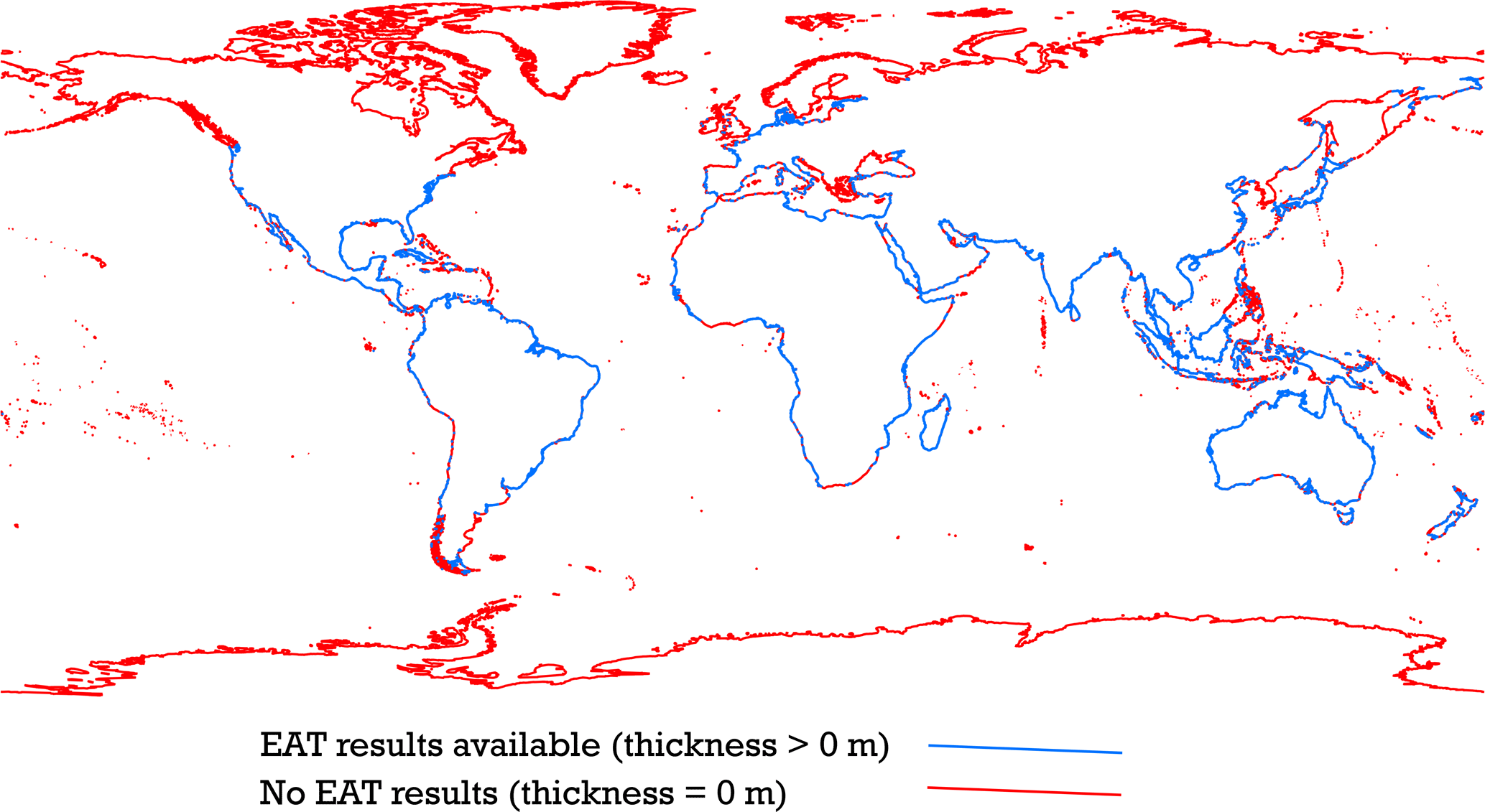
Figure 6 Map showing the spatial distribution of EAT values (unconsolidated sediment aquifer thickness >0 m) and areas where the unconsolidated sediment aquifer thickness is 0 m.

Figure 7 Overall borehole and literature validation results of the EAT results.

3 Results

3.1 Sediment thickness estimation

The aquifer thickness is estimated for 26 968 coastal points around the globe, which cover roughly one-fifth of the global coastline. The rest of the global coastline is covered by other lithological types than unconsolidated sediments and is not taken into account by the ATE method. The overall estimated aquifer thickness (EAT) results are presented in Fig. 5a. It shows that the aquifer thickness estimates range between 0.1 and 5145 m, with a mean value close to 170 m. In total 87 % out of all the EAT values predict a thickness lower than or equal to 300 m (see Fig. 5b). A slightly different result is observed in the literature source analysis, where 69 % of the studied areas have an aquifer thickness lower than or equal to 300 m. This difference is explained by the fact that a disproportionally large number of deltaic areas with thick sediment layers is included in the literature validation dataset. Figure 6 shows the areas where there are no EAT results, largely due to the absence of unconsolidated sediments.

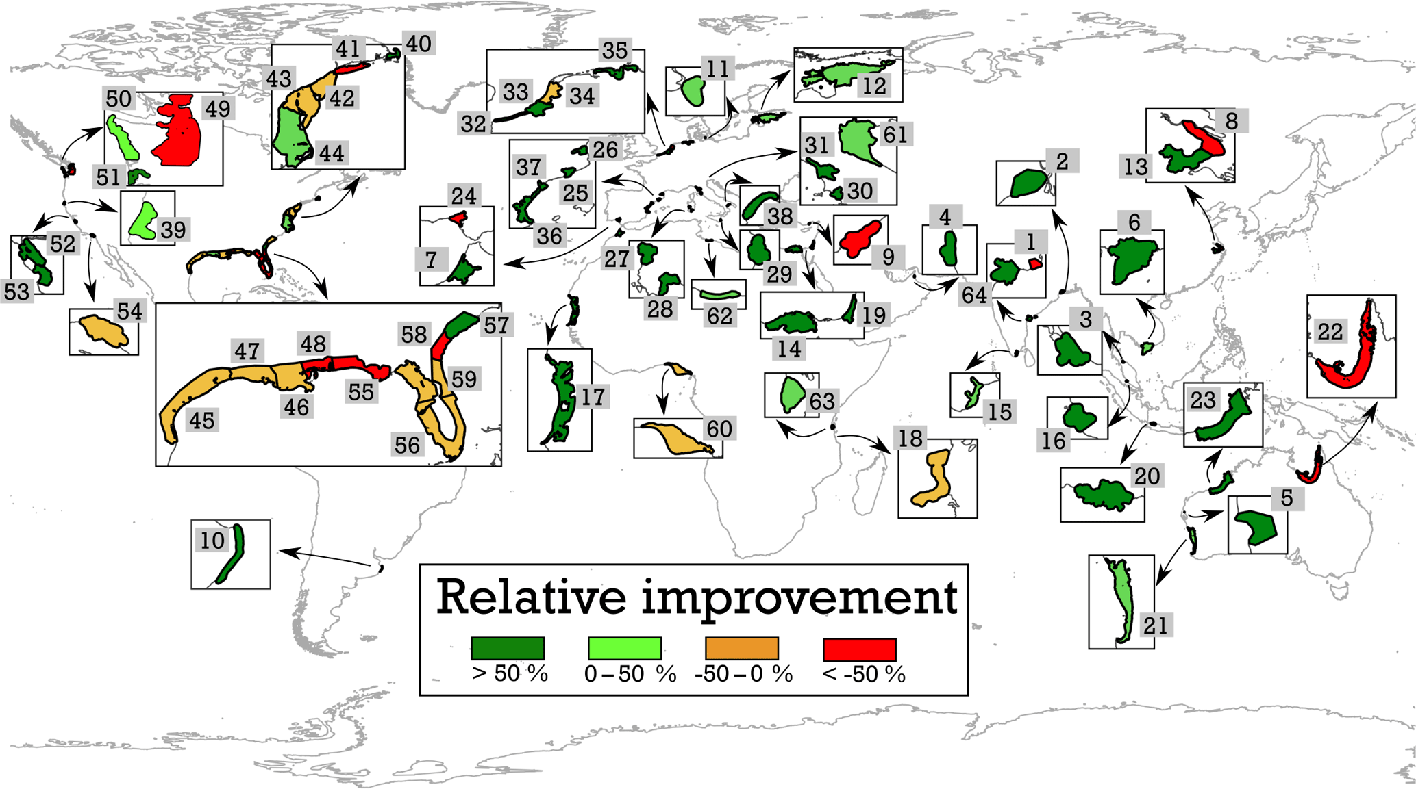
Figure 8 Relative improvement of our estimated sediment thickness compared to using the overall average thickness value from all literature sources.

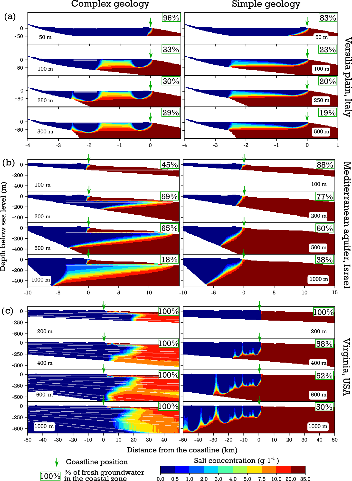
Figure 9 Simulation results as salinity concentration profiles for the cross sections located in the (a) Versilia plain, Italy, (b) Mediterranean aquifer, Israel, and (c) Virginia, USA, with varying aquifer thicknesses and two geology scenarios. The local geological information for each area, (a) Pranzini (2002), (b) Yechieli et al. (2010), and (c) Trapp Jr. and Horn (1997), was implemented (left column) together with a homogeneous aquifer system (right column) to investigate the effects of geological complexity and aquifer thickness on simulated salinity profiles.

3.2 Validation of EAT results

When comparing our EAT with the information collected from the borehole dataset, it is clear that our ATE method provides estimates in the right order of magnitude, but it cannot capture local variations of aquifer thickness. Figure 7a shows that the majority of EAT have relative error values (Eq. 1) lower than 100 %, meaning that our results are of the same order of magnitude as observed values from the borehole dataset. However, the relative improvement of the EAT, as compared with using the average of the borehole thicknesses as an estimate (Eq. 6), is inconclusive as the number of positive values is nearly equal to the total negative values (Fig. 7b).

The results of the validation with the coastal sediment thickness values gathered via a literature review show a more positive result compared to the borehole validation. The overall average thickness of the literature dataset is 353 m, with 69 % of all studied areas having a sediment thickness of 300 m or lower. The relative improvement of sediment thickness estimates using our method is about 22 % compared to the overall thickness value average as indicated by the literature (see Table S3). The relative improvement for individual literature validation areas is shown in Fig. 8. The majority of the areas show an improvement, while estimates for the large coastal plains of the eastern and southern coasts of the USA suggest the opposite. This will be discussed further in Sect. 4. However, in coastal zones that have an average sediment thickness of 300 m or less, the relative improvement of our method is around 59 %. Since our results suggest that 87 % of the global coastline that is composed of unconsolidated sediments has an average thickness of 300 m or lower, the higher relative improvement achieved by our method gains extra importance.

Overall, about 48 % of the validation areas have the absolute relative error percentage below 50 %, while 35 % of validation areas have the absolute relative error percentage between 50 % and 100 % (Fig. 7b). Still, 17 % of the validation areas show an absolute relative error percentage higher than 100 %. A closer look at Fig. 7b reveals that the majority of these validation areas have the average thickness (based on the literature) lower than 100 m. However, the overall results for validation areas with average thickness lower than 300 m show that 59 % have a relative error percentage lower than 50 %: this is an 11 % increase compared to the overall validation dataset.

3.3 Groundwater flow and salt transport modelling

Figure 9 presents a sample of simulated salinity profiles for selected aquifer thickness values for the three test cases. The complete set of the simulated salinity profiles together with the model conceptualization and model parameters and variables is given in Figs. S3 to S6 and Table S5. While comparing the salinity profiles for different aquifer thicknesses, it is apparent that aquifer thickness variations for homogenous geological conditions (figures on the right) do not have large effects on the fresh–saline distribution, except for the lowest aquifer thickness value (Fig. 9a, c). Figure 9b shows that the thicker the aquifer at the coastline, the more saline water intrudes inland and, in some cases, upconing under low-lying areas can be observed (Fig. 9c).

The implementation of complex geological conditions based on the literature description that existed about these sites consisted mainly of introducing low conducting layers (aquitards). As Fig. 9 shows, an aquitard has a substantial effect on the final salinity profile when compared to the salinity profile for homogenous geological conditions with the same aquifer thickness. The aquitard position combined with varying aquifer thicknesses has a large effect on the salinity profile and potential fresh (or brackish) groundwater offshore reserves (Fig. 9b, left column). In particular, the simulations with larger aquifer thickness values show fresh (or brackish) offshore groundwater below the aquitard layer. Similar patterns can be observed in the last test case (Fig. 9c), where the aquitard layers prevent saline water from intruding inland and show large offshore brackish water volumes.

Comparison of fresh groundwater cell percentage within the coastal zone of all three test cases (Fig. 9) shows a trend where the geological scenario (homogenous versus complex) has a larger effect on the amount of estimated fresh groundwater reserves than varying aquifer thickness. For the same geological scenario, the largest differences are observed between the aquifer thickness extreme values (thinnest versus thickest).

4 Data availability

The final output data provide both the EAT at the coastline and the location and depth of the corresponding anchor points. These data are given as shapefile and comma separated value files. The data can be downloaded via https://doi.pangaea.de/10.1594/PANGAEA.880771.

5 Discussion and conclusion

Although in the right order of magnitude (Fig. 7a), the ATE validation with borehole measurements is worse than literature dataset validation. The large scale discrepancy between our global estimated aquifer thickness (EAT) dataset and boreholes is the most obvious cause of this. It shows that our approach is not detailed enough to estimate very local variations in aquifer thickness as picked up by boreholes. Boreholes will generally lie between profile locations, which means that local variation also results in spatial dislocation errors, even though spatial averaging is used to bridge the scale gap (Fig. 4). Still, even when compared to boreholes, we observe an overall ATE method performance improvement for coastal areas with measured thicknesses between 100 and 300 m. The comparison between literature values comes out more favourably, because the data synthesis in the form of spatial statistics and geological profiles is a spatial aggregation form that better matches the ATE method scale. We have used the validation data that could be collected during the course of this study, but the validation set is far from exhaustive. The validation dataset should be expanded and continuously improved to achieve better EAT along the global coastline.

Our method tends to underestimate the aquifer thickness in deeper systems, such as large complex deltaic sedimentary structures with measured average aquifer thicknesses larger than 500 m (Fig. 7). This could be due to the limited cross-section length that spans at most 200 km inland and offshore from the coastline depending on the coastal plain extent. If the latter exceeds this maximum length, then no bedrock formation is found and thus no aquifer thickness is estimated. In case the bedrock formation is only partially taken into account (e.g. only the foothills of a mountain range), its topographical slope will be lower, which leads to lower EAT values at the coastline. The opposite happens for coastal areas with measured average thicknesses lower than 100 m. In these cases, our average EAT values tend to be overestimated (Fig. 7). This could again be caused by the input datasets' resolution (see Table 2) which creates larger errors on local scale and for shallow systems which by themselves have a smaller size than more extensive coastal plains. Compared to the other two datasets providing thickness estimates (de Graaf et al., 2015; Pelletier et al., 2016) the lowest EAT values correspond to the range of values provided by Pelletier et al. (2016). The histogram in Fig. 5b suggests that nearly 20 % of coastal areas covered by our study have EAT between 0 and 50 m. On the other side of the spectrum, our maximum EAT value is 5145 m, which is of the order of magnitude of the de Graaf et al. (2015) dataset.

The numerical modelling results show that only the simulations with extreme EAT values give substantially different results from the simulations with average or close to average EAT values. More variation in the fresh groundwater cells fraction in the coastal zone can be observed in the test case with intermediate aquifer thickness (Fig. 9b). In the other two test cases (Fig. 9a and c) the variation in the fresh groundwater cells fraction is very low for both geological scenarios. On the other hand, the model results also show that geological complexity (multi-layering) has a big impact on the results. Thus, for locally meaningful results, the aquifer thickness is but a first result, and a global estimate of multi-layering (aquifers and aquitards) is a necessary next step. Werner et al. (2013) stress that accounting for geological heterogeneities is important to accurately simulate the saline groundwater distribution in coastal areas. Previous regional- to global-scale studies (e.g. Michael et al., 2013; Solórzano-Rivas and Werner, 2018; Knight et al., 2018) considered the geological conditions (permeability and aquifer thickness) to be homogeneous and our EAT dataset could provide a first constraint on unconsolidated sediment thickness for these types of studies.

When comparing our numerical modelling output (with the complex geology incorporated) with the salinity profiles reported from the individual studies (Pranzini, 2002; Yechieli et al., 2010; Trapp Jr. and Horn, 1997) we find that differences for the cases (a) and (b) are small and a 2-D schematization suffices. However, for cross section (c) the differences are considerable. This is most likely due to the presence of strong alongshore flows in the area, a more complex upper hydrological system and the groundwater withdrawal distribution in the area. This shows that the 2-D modelling approach does not always suffice to estimate coastal groundwater flow.

In conclusion, we showed that it is possible to obtain, at first order, coastal aquifer thickness estimates by using available global datasets and a simple methodology consisting of simulating the bedrock slope from the geological outcrops. Our dataset complements the existing datasets listed in Table 2 by providing an estimate of the complete unconsolidated part of coastal aquifer systems. In such a way it is now possible to build more detailed and vertically stratified regional- and global-scale hydrogeological models based on the herein provided dataset. By combining our dataset with existing sedimentary thickness estimates by e.g. de Graaf et al. (2015) we can distinguish the unconsolidated aquifer system (our dataset) overlaying the sedimentary rocks. However, our dataset is not suitable for building detailed local hydrogeological models, as in such a case additional local geological information should be included. Furthermore, the local-scale geological complexity seems to play a larger role in simulated salinity concentration profiles than aquifer thickness (except for extreme values). Thus, our EAT dataset provides a satisfactory first step towards a global coastal aquifer characterization that should be followed by the assessment of the coastal aquifers' geological complexity for local application.