Probabilistic reconstruction of sea-level changes and their causes since 1900

Coastal communities around the world are increasingly exposed to extreme events that have been exacerbated by rising sea levels. Sustainable adaptation strategies to cope with the associated threats require a comprehensive understanding of past and possible future changes. Yet, many coastlines lack accurate long-term sea-level observations. Here, we introduce a novel probabilistic near-global reconstruction of relative sea-level changes and their causes over the period from 1900 to 2021. The reconstruction is based on tide gauge records and incorporates prior knowledge about physical processes from ancillary observations and geophysical model outputs, allowing us, for the first time, to resolve individual processes and their uncertainties. We demonstrate good agreement between the reconstruction and satellite altimetry and tide gauges (if local vertical land motion is considered). Validation against steric height estimates based on independent temperature and salinity observations over their overlapping periods shows moderate to good agreement in terms of variability, though with larger reconstructed trends in three out of six regions. The linear long-term trend in the resulting global-mean sea-level (GMSL) record is 1.5 ± 0.19 mm yr⁻¹ since 1900, a value consistent with central estimates from the 6th Assessment Report of the Intergovernmental Panel on Climate Change. Multidecadal trends in GMSL have varied; for instance, there were enhanced rates in the 1930s and near-zero rates in the 1960s, although a persistent acceleration (0.08 ± 0.04 mm yr⁻²) has occurred since then. As a result, most recent rates have exceeded 4 mm yr⁻¹ since 2019. The largest regional rates (>10 mm yr⁻¹) over the same period have been detected in coastal areas near western boundary currents and the larger tropical Indo-Pacific region. Barystatic mass changes due to ice-melt and terrestrial-water-storage variations have dominated the sea-level acceleration at global scales, but sterodynamic processes are the most crucial factor locally, particularly at low latitudes and away from major melt sources. These results demonstrate that the new reconstruction provides valuable insights into historical sea-level change and its contributing causes, complementing observational records in areas where they are sparse or absent. The Kalman smoother sea-level reconstruction dataset can be accessed at https://doi.org/10.5281/zenodo.10621070 (Dangendorf, 2024).

1 Introduction

Sea-level rise is one of the most impactful consequences of a warming climate, threatening hundreds of millions of people in low-lying coastal areas (Hinkel et al., 2014). Many of the world's coastal areas are already actively experiencing the impacts of rising sea levels. Along the East and Gulf coasts of the United States, rising seas have resulted in an exponential increase of chronic flooding (Sweet et al., 2022, 2022; Li et al., 2023; Sun et al., 2023), affecting people's daily lives on a now-regular basis. Larger than global rates of sea-level rise around the low-lying Solomon Islands in the Western Pacific have led to severe shoreline recession and the submergence of several islands since the 1930s (Albert et al., 2016). For individual extreme events, such as Superstorm Sandy (New York) or Hurricane Katrina (New Orleans), the underlying (anthropogenic) sea-level rise since the late 19th century has caused significant excess flooding, resulting in more severe impacts than would have occurred in an undisturbed climate (Irish et al., 2014; Strauss et al., 2021). In Africa, 20 % of the heritage sites of Outstanding Universal Value are currently at risk of a 1-in-100-year coastal extreme event, and the number of sites is projected to triple by 2050 under continued sea-level rise (Vousdoukas et al., 2022). These examples underscore that understanding historical sea-level rise and its individual contributing factors is critically important to better project future climatic changes and the resulting impacts along the coast.

Since 1992, radar altimeters on board of satellites have continuously monitored sea-surface height changes with near-global coverage and an accuracy of 2–3 cm locally (Ablain et al., 2015). The resulting record of global-mean sea-level (GMSL) change indicates a significant increase of about 3.4 mm yr⁻¹ since 1993, with an underlying acceleration of about 0.09 mm yr⁻² (Nerem et al., 2018). Moreover, the magnitude of the spatial variability in the rates of rise can be significantly larger in some regions than the GMSL estimate (Wahl and Dangendorf, 2022), indicating that for local coastal-planning-and-adaptation purposes, local sea-level information, as provided by satellites, is of the utmost importance. However, the current satellite record has three major limitations. First, it is only available for 30 years, a period that is still too short to unambiguously detect the emergence of climatic trends and accelerations at a local level (Haigh et al., 2014). Second, sea-surface measurements are more accurate in the open ocean than close to the coast (e.g., Cazenave et al., 2022). Third, its measurements only provide information about changes within the ocean itself (i.e., the absolute sea level), not the coastal land. The combination of absolute sea level and vertical land motion (VLM) (i.e., the relative sea level), however, is the most relevant to decision makers in the coastal zone. Measurements of relative sea level over periods longer than the satellite record are provided by tide gauges, including those in some locations such as Amsterdam (van Veen, 1945), Stockholm (Ekman, 1988), or Brest that have records spanning several hundred years (Woodworth et al., 2010). Tide gauges have been measuring sea level at several thousand locations worldwide, and, with the exception of a few island locations, these records are limited to the coastal zones of the continents (Church and White, 2011).

Scientists have therefore developed mathematical approaches to reconstruct the geometry of sea level from the sparse tide gauge records. One approach, which is based on reduced spatial optimal interpolation (RSOI), determines the spatial patterns of sea-surface height from satellite altimetry via empirical orthogonal functions and then fits the leading patterns to the sparse tide gauge record, providing a spatiotemporal reconstruction of sea level with the same spatial resolution as satellite altimetry and a length similar to tide gauge records (e.g., Church et al., 2004; Church and White, 2006; Church and White, 2011; Ray and Douglas, 2011; Meyssignac et al., 2012). The second approach, which uses a Bayesian framework and ensemble Kalman smoothing (Hay et al., 2013, 2015, 2017), employs spatial patterns of individual sea-level contributors known a priori, such as ice melt (the so-called fingerprints of gravitation, rotation, and deformation: GRD), glacial isostatic adjustment (GIA), and the modeled sterodynamic (i.e., the combination of steric expansion and ocean circulation changes) sea level from climate models that are fitted to the tide gauge records. Both approaches provide GMSL estimates that agree well with satellite altimetry trends over the overlapping periods since 1993, but their GMSL estimates differ before the 1970s. The Kalman-smoother-based technique indicates a lower trend (∼1.2 ± 0.2 mm yr⁻¹) than the RSOI-based techniques (1.6–1.9 mm yr⁻¹) before 1990, thus leading to a larger acceleration over the entire 20th century (Hay et al., 2015). Recent assessments based on different reconstruction techniques have indicated that the distinct treatment of VLM at tide gauges may be a plausible explanation of the inconsistent trends before 1990 (Dangendorf et al., 2017; Frederikse et al., 2020). While VLM unrelated to GIA was not accounted for in earlier RSOI reconstructions (Church et al., 2004, 2006; Church and White, 2011; Ray and Douglas, 2011; Meyssignac et al., 2012), the Kalman-smoother-based approach accommodates possible VLM unrelated to GIA as local effects in a residual term that does not affect the final estimation of GMSL (Hay et al., 2017).

Both approaches are also affected by distinct types of uncertainties related to the representation of regional sea-level variability. While the RSOI reconstructions often provide a good representation of interannual variability (Calafat et al., 2014; Dangendorf et al., 2019), they have limitations that are rooted in the assumption that major modes of variability can be robustly determined by the short satellite record and that the corresponding spatial patterns remain stationary in time (Christiansen et al., 2010, Calafat et al., 2014). It is now well established that modes of variability can extend over periods much longer than the satellite record (Chambers et al., 2012; Dangendorf et al., 2014b) and that different contributing factors to sea level, such as sterodynamic changes or ice melt, vary in space and time (Marzeion et al., 2012; Frederikse et al., 2020). Consequently, the resulting regional trends over their overlapping period from 1960 to 2007 vary widely between available RSOI reconstructions (Carson et al., 2017). The Kalman smoother generally overcomes the non-stationary modes in the RSOI-based technique by estimating the individual GRD fingerprints directly from the tide gauge record at each time step and by using sterodynamic priors from the ocean components of climate models. However, the GRD fingerprints co-vary between different source regions such that, especially in the presence of large sterodynamic variability (Dangendorf et al., 2021), their separation becomes a low signal-to-noise challenge (Hay et al., 2017). This limitation is further exacerbated by the fact that the sterodynamic priors from climate models are not in phase with observations, since climate models all start from their own initial conditions (Fasullo and Nerem, 2018). Thus, there is limited skill in reducing the noise for the detection of GRD fingerprints at interannual to decadal scales. While this has been demonstrated to have minor effects on the estimation of GMSL, the inability to separate the various GRD fingerprints propagates into the resulting regional fields and hampers the separation into individual sea-level contributors (Hay et al., 2017).

Here, we introduce a new reconstruction that leverages the strengths of both approaches. Since the original publications of the Kalman smoother approach (Hay et al., 2013, 2015), independent estimates of historical GRD fingerprints and corresponding uncertainties have become available (Frederikse et al., 2018, 2020, and references therein), making their estimation from tide gauge records no longer mandatory. Instead, we pre-describe the entire history of contemporary barystatic GRD fingerprints (glaciers, ice sheets, and terrestrial sources) and their uncertainties with an ensemble based on Frederikse et al. (2020). We also consider inverse barometer effects (IBEs) and prescribe the priors of the spatial pattern of sterodynamic sea-level change by using an ensemble of RSOI reconstructions from tide gauges after the removal of GRD, GIA, and IBE estimates. The adjustments have two main advantages: first, the reconstruction of sea level at regional and global scales is reduced to the sterodynamic component (and associated residual effects that are not properly captured by the other components), effectively avoiding any co-variance and low signal to noise associated with distinguishing the individual fingerprints. Second, the approach enables the estimation of the individual contributors and sea-level change as constrained by tide gauges. As such, we derive a novel global and regional-mean sea-level reconstruction at annual resolution covering the period from 1900 to 2021, extending the reconstructions from Hay et al. (2015) and Dangendorf et al. (2019) by 11 and 6 more years, respectively. We demonstrate that the new reconstruction accurately reconstructs sea level from satellite altimetry and tide gauges and provides a novel estimate of the sterodynamic component that is independent of temperature and salinity observations.

2 Methodology and data

2.1 Methodology

Hay et al. (2013, 2015, 2017) developed a Kalman smoother approach that calculates posterior estimates of GMSL and associated regional sea-level fields from sparse tide gauge records. In the following, we closely follow the methodological description in Hay et al. (2017), which is also summarized in Fig. 1. The Kalman smoother is conditioned on a set of different prior sea-level fields that represent the individual processes contributing to relative sea-level change (sterodynamic sea level, barystatic GRD, and GIA) and can be divided into three analysis steps: a forward-filtering pass, a backward smoother pass, and a multi-model ensemble component (Hay et al., 2017). The Kalman filter incorporates several equations that can be separated into two groups of time and measurement update equations (Kalman, 1960). In the time update equations, a prior estimate of sea level at time step k is estimated based on the state of the system at time k−1. The state vector ${\widehat{\mathit{x}}}_k$ and the associated covariance P_k are predicted moving forward in time using the state transition matrix φ and the control input parameters Bu_t:

$$\begin{array}{}\text{(1)}& {\displaystyle }{\widehat{\mathit{x}}}_k^{-}=\mathit{\phi }{\widehat{\mathit{x}}}_{k-\mathrm{1}}+{\mathbf{Bu}}_k\text{(2)}& {\displaystyle }{\mathbf{P}}_k^{-}=\mathit{\phi }{\mathbf{P}}_{k-\mathrm{1}}{\mathit{\phi }}^T+\mathbf{Q}.\end{array}$$

Here, Q is the process noise covariance, and the superscript minus sign indicates that the estimates are based on the prior state of the system from the time update. The state vector ${\widehat{x}}_k$ contains estimated sea levels at 516 tide gauge sites (see Sect. 2.2 for more details on the selection of input data), 74 742 satellite altimetry locations, and an estimate of globally uniform GMSL change. The reduction of the vector to only one globally uniform GMSL estimate is the first modification to Hay et al. (2015, 2017), where the vector also contained estimates of 21 melt rates from mountain glaciers and ice sheets. The second modification is related to the input control parameters, which comprised modeled estimates of sea-level contributions from GIA and ocean dynamics in Hay et al. (2015, 2017). Here, we replace the input control parameters by a combination of model estimates of GIA (Caron et al., 2018), total barystatic GRD (Frederikse et al., 2020), IBEs, and sterodynamic sea-level change. The sterodynamic component is pre-calculated using an ensemble of RSOI reconstructions (Calafat et al., 2014) that take the 10 leading modes of variability from empirical orthogonal functions estimated from satellite altimetry and fit them to a subset of tide gauge records. Both the satellite altimetry and tide gauges are corrected for the effects of GIA, barystatic GRD, and IBEs before performing the RSOI, therefore reducing the RSOI reconstructions to solely the sterodynamic component of sea-level change (and possible residual processes that are not properly captured by the other processes). Note that the RSOI is performed without the spatially uniform zero matrix (introduced by Church et al., 2004, to preserve the long-term trend in GMSL), as we are solely interested in reconstructing regional and global variability. Low-frequency changes (including the trend) of global mean steric sea-level change are estimated in the Kalman smoothing process. The resulting sterodynamic sea-level fields are then used as input parameters for the Kalman smoother. The state transition matrix φ describes prior beliefs about how sea-level rates vary from one time step k to another. It also contains information about the spatial patterns of sea-level change that connect the global mean to any given locality.

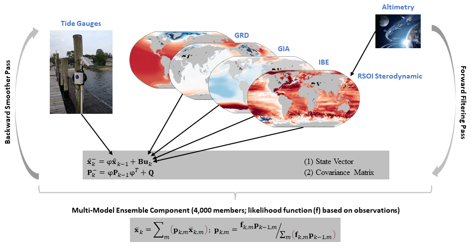
Figure 1 Schematic representation of the Kalman smoother and the respective inputs used for the reconstruction of sea level and its causes. Both photographs were taken from https://creativecommons.org (last access: 24 May 2024) and are in the public domain. The altimetry photo (provided by NASA JPL) can be found at https://flic.kr/p/CbBqMG (last access: 24 May 2024). The tide gauge photo (taken by Monique Lafrance Bartley, URI GSO) can be found at https://flic.kr/p/yqS6fK (last access: 24 May 2024).

During the measurement update, prior estimates of ${\widehat{\mathit{x}}}_k$ and P_k are conditioned upon tide gauge observations stored in z_k at time step t_k to identify a linear combination of the prior estimate ${\widehat{\mathit{x}}}_k^{-}$ and a weighted difference between observations and predictions ${\widehat{\mathbf{H}\mathit{x}}}_k^{-}$, where H is a matrix that maps the state vector and covariance into the observation space:

$$\begin{array}{}\text{(3)}& {\widehat{\mathit{x}}}_k={\widehat{\mathit{x}}}_k^{-}+{\mathbf{K}}_k({\mathbf{z}}_k-\mathbf{H}{\widehat{\mathit{x}}}_k^{-})\end{array}$$

and

$$\begin{array}{}\text{(4)}& {\mathbf{P}}_k=(\mathbf{I}-{\mathbf{K}}_k\mathbf{H}){\mathbf{P}}_k^{-}.\end{array}$$

I is the identity matrix, and K_k is the Kalman gain matrix, defined as follows:

$$\begin{array}{}\text{(5)}& {\mathbf{K}}_k={\mathbf{P}}_k^{-}{\mathbf{H}}^T({\mathbf{HP}}_k^{-}{\mathbf{H}}^T+\mathbf{R}{)}^{-\mathrm{1}},\end{array}$$

where R is the observation noise covariance matrix (Kalman, 1960). The observation noise covariance matrix R is calculated using an expectation-maximization approach, which identifies the covariance for all 516 tide gauge records in the presence of data gaps using an iterative maximum likelihood estimate (Schneider, 2007). To avoid large biases due to data gaps, the algorithm is only applied to data after 1955, after which data gaps significantly decrease. Further details on the calculation of R can be found in the supplementary information of Hay et al. (2013).

After the forward pass, the filter is run backwards in time, and a linear combination of the forward and backwards passes is calculated to ensure that the posterior estimates of the state vector and its covariance over the entire time window (here 1880 to 2021, although we only present results since 1900 to avoid drifts, following Hay et al., 2015) are conditioned upon all observations (Gelb, 1974).

The last step comprises the ensemble multi-model component, in which the forward and backwards passes are calculated for all possible prior combinations. Here, we consider 40 different GIA models, 100 GRD realizations, and 1 IBE product, resulting in a total of 4000 different combinations (i.e., also 4000 different RSOI realizations) considered in the multi-model component. The likelihood of each combination of models is calculated based on available observations (see Hay et al., 2013, for details), and a weighted sum of results is obtained. It is this weighted sum that represents the final ensemble multi-model Kalman smoother GMSL estimate and the associated regional field. As outlined in Hay et al. (2013, 2017), a residual term in the Kalman smoother allows the modeling of local effects at individual tide gauge sites (e.g., VLM unrelated to GIA or possible datum shifts), but this term is not included in the computation of GMSL and the associated regional field.

The Kalman smoother provides a rigorous probabilistic framework for the propagation of observational and model errors. In this current version, uncertainties σ are determined by P_k for each individual tide gauge and the resulting GMSL estimates. The uncertainty at each of the 74 742 grid points of the regional sea-level fields is determined by the underlying ensembles of the 4000 different sea-level contributor fields, considering their probability weights plus the spatially uniform uncertainty from the GMSL estimation. Further details on the Kalman smoother technique can be found in Hay et al. (2013, 2015, 2017). Readers who are interested in further details of the RSOI technique are referred to Calafat et al. (2014).

2.2 Data

We use 516 globally distributed annual tide gauge records from the online portal of the Permanent Service for Mean Sea Level (PSMSL) in Liverpool (Holgate et al., 2013) that provide at least 20 years of data and are located south of 67° north (thus ignoring the uncertain records in the Russian Arctic; Hamlington and Thompson, 2015). We also performed an additional visual screening of the records that fulfill the former criteria. Sites that are obviously affected by strong nonlinear VLM due to either earthquakes (e.g., many sites around Japan or Ko Lak in Thailand after the 2004 tsunami) or fluid withdrawals (e.g., in Louisiana and Texas) are either entirely discarded or only portions of their records are considered (e.g., Manila before the 1960s). All tide gauges, along with their geographical locations and temporal availability, are shown in Fig. 2.

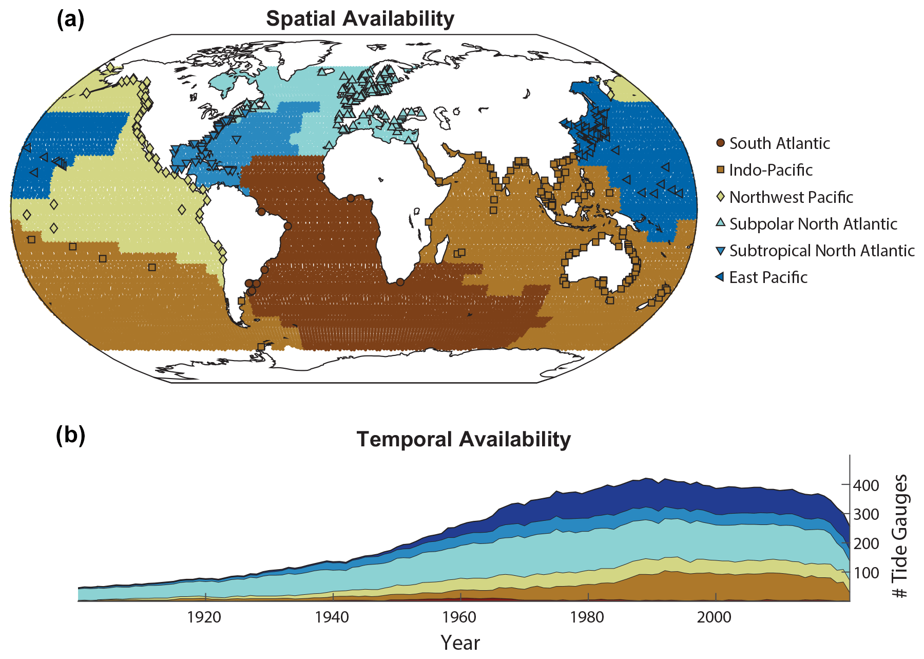
Figure 2 Global map of tide gauges used in this study and their net availability over time. (a) Tide gauges are shown as black-edged markers with colors representing different regions. The colored areas on the map represent the six regions used for basin-scale averages described in Thompson and Merrifield (2014). (b) The corresponding availability as a function of time, differentiated for each region.

For GIA, we consider 40 models taken from the ensemble published by Caron et al. (2018), who calculated GIA uncertainties using Bayesian techniques for an ensemble of 128 000 forward models based on varying 1-dimensional Earth structures and ice histories. Thirty of the GIA models were selected based on similar statistics of the large ensemble; that is, they were selected such that their median and standard deviation matches that of the large ensemble (Lambert Caron, personal communication, 2023). We also added the 10 best-performing models based on their likelihoods, as inferred from a comparison to a global navigation satellite system (GNSS) and relative sea-level records in Caron et al. (2018). We consider the relative sea level (for tide gauge records) and sea-surface height outputs (for satellite altimetry) from the models.

Instead of calculating melt rates from tide gauge records within the Kalman smoother framework, we incorporate recently published barystatic GRD estimates from Frederikse et al. (2020). The estimates have been updated to 2020 (Thomas Frederikse, personal communication, 2023); therefore, the data were extrapolated to the year 2021 based on a linear fit to the last 5 years at each grid point (using either a linear or a quadratic fit does not significantly affect the extrapolation over 1 year). The GRD ensemble consists of 100 representative members (again, these were chosen such that they have a similar median and standard deviation to the 5000-member ensemble from Frederikse et al., 2020) that combine mass changes from glaciers (Parkes and Marzeion, 2018; Zemp et al., 2019), ice sheets (Kjeldsen et al., 2015; IMBIE team, 2018; Bamber et al., 2018; Adhikari et al., 2019; Mouginot et al., 2019), and terrestrial water storage, including hydrology (Humphrey and Gudmundsson, 2019), water impoundment in artificial reservoirs (Chao et al., 2008), and groundwater depletion (Döll et al., 2014; Wada et al., 2016). Here, the sum of the individual contributions is considered.

IBE variations are derived from sea-level pressure data from atmospheric reanalysis models, specifically the 20th Century Reanalysis v3 covering the period from 1900 to 2015 (Slivinski et al., 2019) and the NCEP-NCAR reanalysis 1 (Kalnay et al., 2018) from 2016 to 2021. Both reanalyses are interpolated from different global grids onto the 74 742 grid points for the regional sea-level fields considered in the Kalman smoother. They are combined after adjusting them to the same mean at each grid point over the 5 overlapping years between 2011 and 2015. The choice of using the 20th Century Reanalysis v3 is based on its availability over long periods. Other datasets (e.g., HADSLP) are not considered, as the IBEs make only a very minor contribution compared to other processes, and every additional dataset would double the total ensemble size considered here. IBEs are calculated from the combined and interpolated sea-level pressure fields as follows:

$$\begin{array}{}\text{(6)}& {\mathit{\mu }}^{\text{IBE}}=-{\displaystyle \frac{P_{\mathrm{a}}-{\stackrel{\mathrm{‾}}{P}}_{\mathrm{a}}}{\mathit{\rho }g}},\end{array}$$

where μ^IBE is the inverted barometer contribution to sea level, P_a is the atmospheric pressure at sea level (the overbar represents the spatial average over the global ocean surface: ∼1013 hPa), ρ is a constant reference ocean density, and g is the acceleration due to gravity (Ponte, 2006).

Satellite altimetry is required for the calculation of the RSOI reconstruction of residual sea level, which is interpreted as sterodynamic. Here we use monthly sea-surface height fields from the Copernicus Marine Environment Monitoring Service (CMEMS) (Copernicus Climate Change Service, Climate Data Store, 2018), which are available on a global grid of 0.25° resolution and cover the period from 1993 to 2021. To make the satellite data comparable to the relative sea level at tide gauges, we add the dynamic atmospheric correction that represents IBE variations at timescales longer than 20 d (Ponte and Ray, 2002) and the deformational component of barystatic GRD (Frederikse et al., 2020). We also correct the satellite record for a globally uniform drift of about −1.5 mm yr⁻¹ (from the TOPEX mission) before 1999 following WCRP Global Sea Level Budget Group (2018). At higher latitudes, we fill data gaps due to seasonal sea ice using a data interpolating empirical orthogonal function (DINEOF) approach (in addition to Coulsen et al., 2022; Beckers and Rixen, 2003) if the records provide at least 50 % data coverage over the entire period. We then build annual averages based on the gap-filled monthly data. For computational reasons, we only consider every fourth grid point, leaving us with a total of 74 742 locations.

3 Results

3.1 Validation

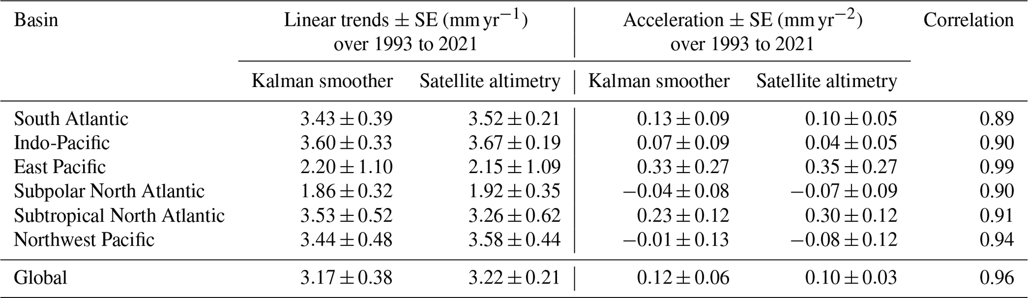
The GMSL and basin-scale averages (based on basin definitions following Thompson and Merrifield, 2014) of the new reconstruction of relative sea level and its individual contributors are presented in Fig. 3. Overlaid are the global and regional averages from satellite altimetry. We note that covariance information from satellite altimetry was used to determine the sterodynamic component in the reconstruction, and, as such, the validation here is not fully independent. The correlations between (detrended) basin-scale averages of the reconstruction and satellite altimetry observations are all larger than r=0.89, with maximum values of r=0.99 in the eastern Pacific (Table 1). The high level of agreement between both products also holds at the local level, which is demonstrated by the correlation map in Fig. 2a. The median correlation over all of the oceans worldwide is about r=0.87, with more than 95 % of all grid points having a correlation coefficient of 0.7 or higher. In general, correlations are highest closer to the coast and in tropical latitudes in the Pacific and Indian oceans. The higher correlation along coasts may be related to propagating signals that induce coherence over large distances and are often linked to large-scale modes of variability (Hughes et al., 2019). The high correlations in tropical latitudes in the Pacific and Indian oceans are due to the dominant influence of Pacific climate variability (the El Niño–Southern Oscillation and Pacific Decadal Oscillation) on regional sea levels worldwide (Hamlington et al., 2013). The lowest correlations are found, as is common in other spatiotemporal reconstructions (Carson et al., 2017; Dangendorf et al., 2019), along the pathways of major ocean circulation systems such as the Gulf Stream, the Kuroshio, or the Antarctic Circumpolar region. This is because those areas are characterized by considerable small-scale variability due to the presence of mesoscale eddies, which reduces, in combination with the sparse sampling of tide gauges, the skill of the reconstruction. The reconstruction is also meant to primarily capture large-scale patterns by reducing it to the 10 major modes. However, this eddy-related noise averages out at the basin scale, leading to consistently larger correlation coefficients (Table 1).

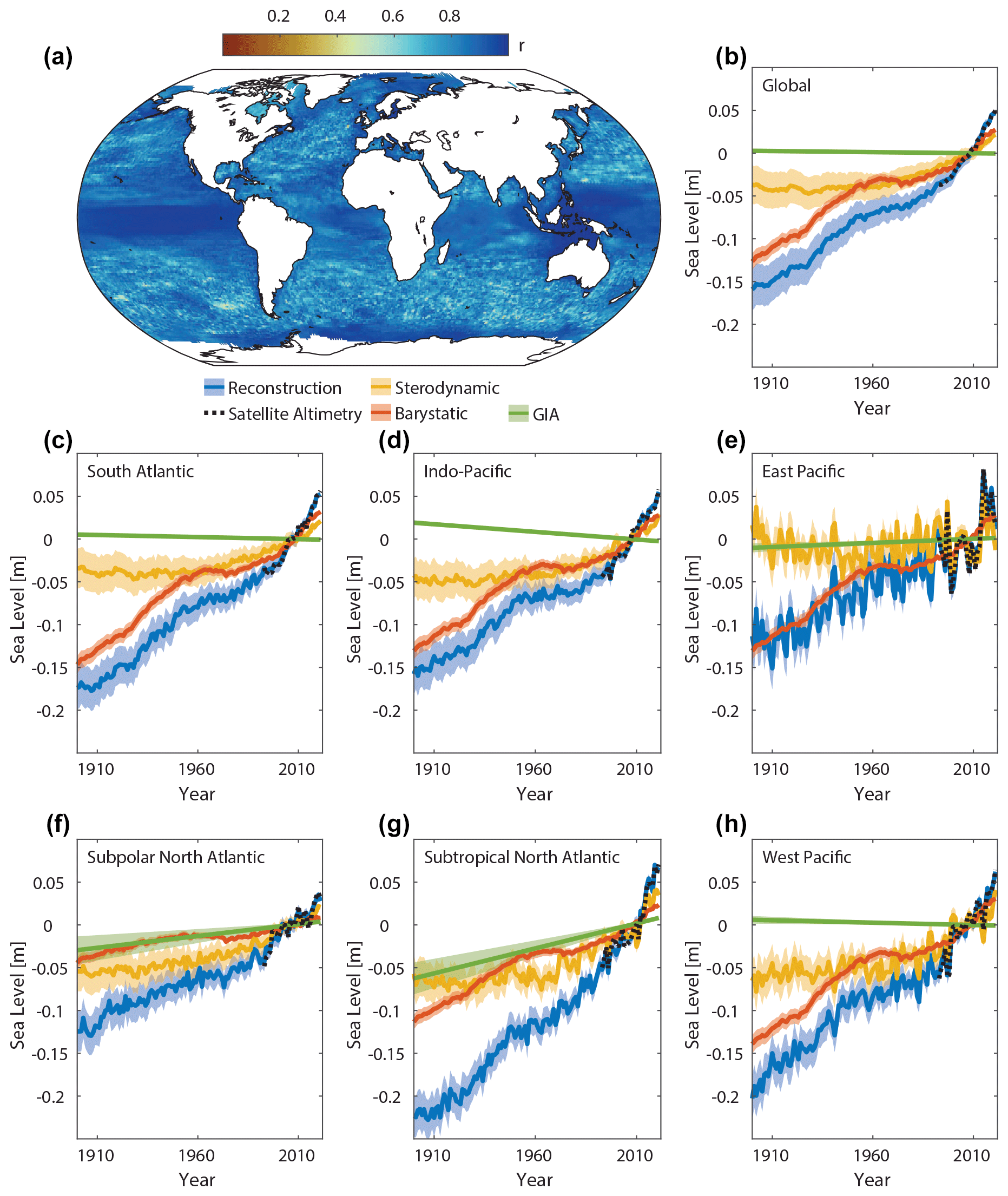
Figure 3 Global and regional reconstructed sea-level changes, their contributing causes, and a comparison to observations from satellite altimetry. Shown are the Pearson correlation coefficient between the (detrended) new reconstruction and (detrended) satellite altimetry at each grid point over the world's oceans over the overlapping period from 1993 to 2021 (a) and the time series of global (b) and regional (basin-scale) (c–h) sea levels and their causes. In (b–h), the satellite altimetry record is shown for comparison as well. Uncertainties are shown as shaded regions.

Table 1 Linear trends in global and basin-scale sea levels from the Kalman smoother and satellite altimetry over 1993 to 2021. All trends have been calculated based on ordinary least-squares regression. Trend uncertainties are presented as the standard errors (SEs) calculated assuming that the residuals are autocorrelated and can be reasonably well approximated by an autoregressive process of order 1. They also contain the reconstruction uncertainty. Also shown are the respective correlation coefficients calculated from the detrended global and basin-scale averages.

The good correspondence between the new reconstruction and satellite altimetry is not only limited to the variability; it is also visible in the linear trend and acceleration maps (including the solid-earth component of barystatic GRD and relative sea-level signals of GIA as determined by the Kalman smoother, which has been added to the satellite altimetry) over their overlapping period from 1993–2021 (Fig. 4). The spatial pattern correlation between the two resulting maps for trends and acceleration coefficients (both estimated via ordinary least squares) is r=0.97 and r=0.92, respectively. There is no systematic bias between observed and reconstructed trends and accelerations, which is reflected in median differences of about 0.04 mm yr⁻¹ and −0.01 mm yr⁻², respectively. A total of 95 % of all locations worldwide show differences in trends and accelerations that are smaller than absolute values of 0.85 mm yr⁻¹ and 0.26 mm yr⁻², respectively (Fig. 4). The majority of the trends (98.9 % of the entire ocean area) and accelerations (96.5 % of the entire ocean area) in the residuals (satellite observations minus reconstruction) are also not statistically significant, and the few that are statistically significant do not cluster in a specific region. Again, at the basin scale, those differences are even smaller (Fig. 3, Table 1).

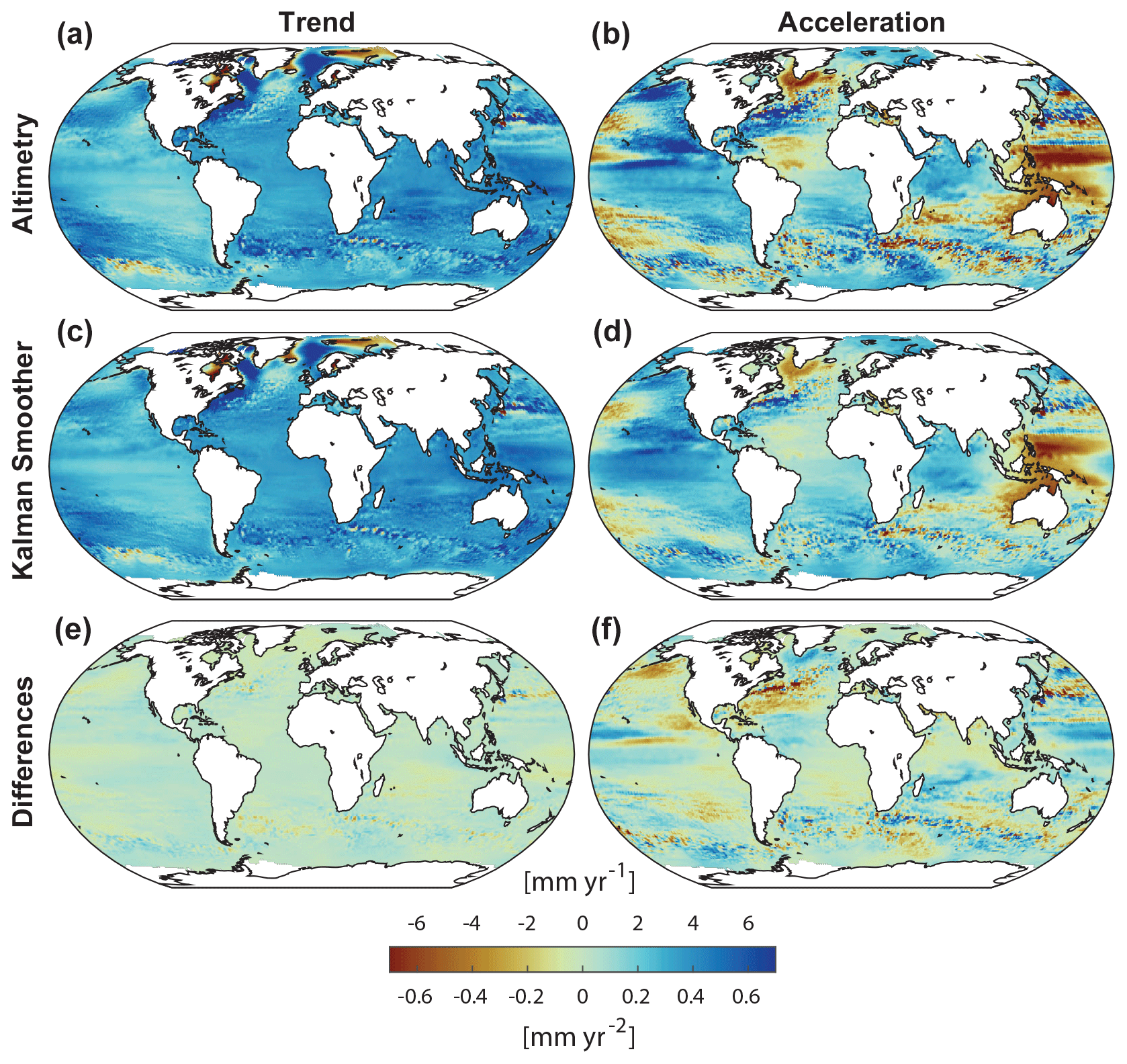
Figure 4 Trends and accelerations from satellite altimetry and the reconstruction over 1993 to 2022. Trends (a, c, e) and accelerations (b, d, f) as determined by satellite altimetry (a, b) and the reconstruction (c, d). Also shown are the differences between the two products (satellite altimetry minus reconstruction: e, f). Note that all trend maps show relative sea-level trends and thus include the relative sea-level change signal of GIA as determined within the Kalman smoother reconstruction. The pattern correlation between the two trend maps is r=0.97, and that between the two acceleration maps is r=0.92. The rms difference is 0.43 mm yr⁻¹ and 0.13 mm yr⁻², respectively. Note that the trend and acceleration differences are insignificant over 98.9 % and 96.5 % of the global ocean, respectively.

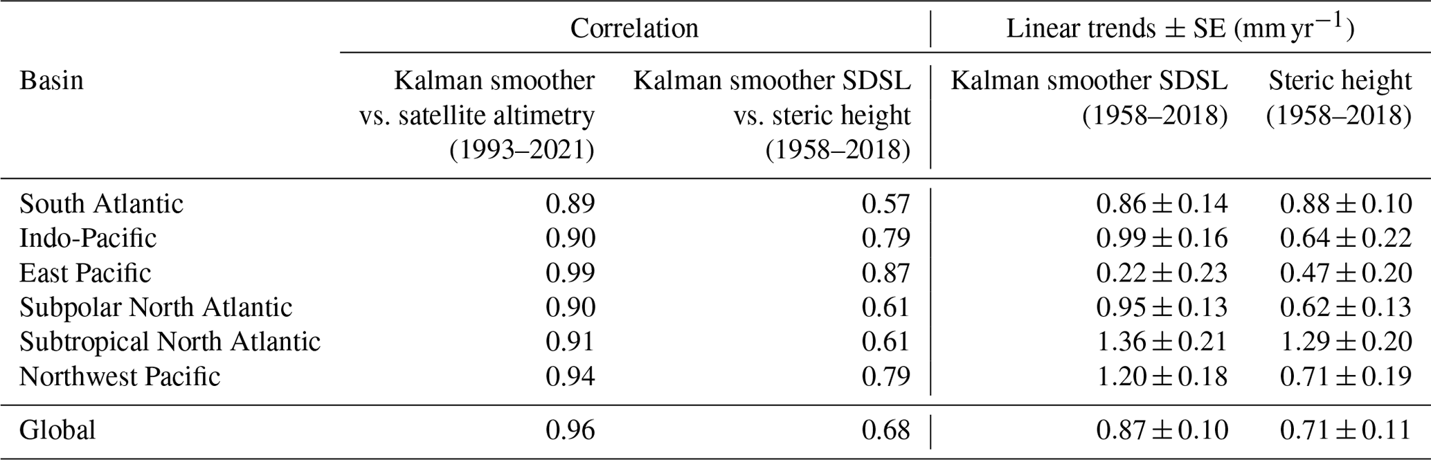
An additional independent way of testing the performance of the new reconstruction is by assessing the inferred sterodynamic component against independent estimates of steric height as derived from temperature and salinity observations. Here we make use of various global (WCRP Global Sea Level Budget Group, 2018; Frederikse et al., 2020; Camargo et al., 2020) and basin-scale (Frederikse et al., 2020) estimates, all of them based on ensembles of different products. An important consideration here is that a comparison between steric and sterodynamic height is only straightforward at basin or global scales, as the former does not contain any manometric signals due to ocean circulation changes (Bingham and Hughes, 2012; Dangendorf et al., 2021). At the basin scale, manometric sea-level changes (that manifest in the ocean-bottom pressure) are thought to be a minor contribution at interannual and longer timescales (Frederikse et al., 2020), while they entirely cancel out at the global scale. The results of the comparison are summarized in Fig. 5 and Table 2. Linear trends agree within their respective uncertainties everywhere during the overlapping period from 1958 to 2018 (considering 95 % confidence levels, i.e., 2 times the standard error given in Table 1), except for the northwest Pacific and the subpolar North Atlantic, where the Kalman smoother reconstruction produces (mean) sterodynamic trends that are 169 % (0.49 mm yr⁻¹ difference) and 153 % (0.33 mm yr⁻¹) larger than those from the steric height fields based on temperature and salinity observations. Although they agree within their uncertainties, trends in the Indo-Pacific region are also overestimated by 154 % (0.35 mm yr⁻¹) by the Kalman smoother reconstruction. There are several possible reasons for that mismatch. The reconstruction in the northwestern Pacific primarily relies on tide gauges that are situated in areas of high seismic activity (Oelsmann et al., 2024). While we have screened the dataset before its inclusion in the reconstruction, we cannot rule out that residual signals propagate into the reconstruction of the spatial portion of the sterodynamic component as determined by the RSOI. Furthermore, both regions, and specifically the subpolar North Atlantic, contain large shallow continental-shelf seas in which ocean-bottom pressure changes (i.e., manometric sea-level changes) dominate the sterodynamic variability (Landerer et al., 2007). Thus, the larger trends may also indicate an increase in wind-driven manometric changes on the shallow shelf that would not be seen in the steric height alone. Indeed, large portions of the northwestern European shelves have experienced positive trends due to shifts in the North Atlantic Oscillation and the corresponding westerly winds over the second half of the 20th century (Dangendorf et al., 2014a; Gräwe et al., 2019). As a test, we calculated the basin average in the subpolar North Atlantic with and without the northern European shelf. The trend without the northern European shelf was ∼0.1 mm yr⁻¹ smaller than the trend with it, thus explaining a maximum of ∼30 % of the total difference. A similar test in the northwestern Pacific did not yield any significant trend differences. Finally, we use the outputs from 1-dimensional GIA models (Caron et al., 2018) within the Kalman smoother framework, which may perform reasonably on a global scale but are characterized by larger uncertainty locally (Thompson et al., 2023). Thus, a fraction of the mismatch in the subpolar North Atlantic might also arise from the propagation of uncertainties in GIA models into the sterodynamic reconstruction. Lastly, we note that temperature- and salinity-based steric-height products are deeply uncertain as well (e.g., MacIntosh et al., 2017; Rietbroek et al., 2016; Cheng et al., 2017) and contain only very little information about the deep ocean below 2000 m. Overall, however, the agreement between the two products is therefore reasonable. This is also reflected in correlations which range from r=0.57 in the South Atlantic to r=0.87 in the East Pacific, indicating a moderate to strong agreement in the variability in all basins (Table 2). Similar conclusions can be drawn for the global mean. The linear trends between the Kalman smoother reconstruction and different steric-height estimates agree within their respective uncertainties (the central trend in the Kalman smoother reconstruction is only 0.17 mm yr⁻¹ larger than the ensemble mean from Frederikse et al., 2020), and the variability is significantly correlated (r=0.68) over the period from 1958 to 2018. Before 1958, the global average from Frederikse et al. (2020) is based on only one available reconstruction from Zanna et al. (2019). Both show some similarities in the first decades of the 20th century, although the steric-height estimate from Zanna et al. (2019) exhibits slightly stronger and more enhanced warming in the 1930s than the Kalman smoother estimate from tide gauges (Fig. 5a). Again, those differences are largely within the respective error bars.

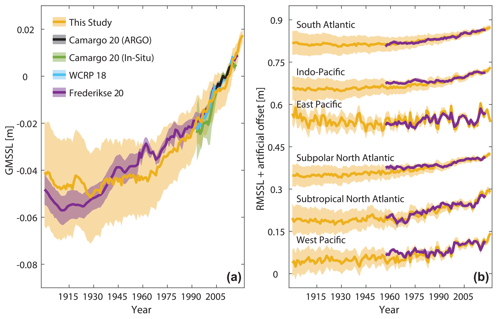
Figure 5 Comparison between observed steric and reconstructed sterodynamic global and regional mean sea levels. (a) Global mean (thermo-)steric sea levels from different observational products based on temperature observations versus the new estimate from the reconstruction. (b) Basin-scale regional averages of steric height from observational products (Frederikse et al., 2020), and the new sterodynamic estimate from the reconstruction. Uncertainties are shown as shaded regions.

Table 2 Performance metrics of the Kalman smoother reconstruction. Shown are the linear correlation coefficients between detrended basin-scale and global averages of sea level from the Kalman smoother reconstruction and satellite altimetry as well as the sterodynamic sea-level (SDSL) component from the Kalman smoother reconstruction and the steric height from Frederikse et al. (2020) (left). Also shown are the linear trends in the latter two over their overlapping period from 1958–2018. Trend uncertainties are shown as standard errors calculated assuming that the residuals are autocorrelated and can be reasonably well approximated by an autoregressive process of order 1. They also contain the reconstruction uncertainty.

Next, we look at individual tide gauge sites and compare them with the time series of the nearest-neighbor grid point from the weighted fields of the Kalman smoother reconstruction and satellite altimetry. Figure 6a–g show seven sites distributed worldwide: San Francisco (United States), Brest (France), Nagasaki (Japan), Honolulu (Hawaii), La Libertad (Ecuador), Fremantle (Australia), and Chuuk, Moen Island (Micronesia). We note that the nearest-neighbor time series from the weighted fields of the Kalman smoother do not contain the residual term from the Kalman smoother and are thus purely the result of the known modeled processes (i.e., the sum of sterodynamic sea level, barystatic GRD, IBEs, and GIA) at each location (Hay et al., 2017). At all seven locations, the nearby reconstruction provides a good representation of the interannual variability, which is reflected in strong correlation coefficients that range from r=0.75 in Brest to r=0.91 in Weno. Linear trends over their overlapping periods agree within their respective uncertainties, and trend differences are smaller than 0.6 mm yr⁻¹ everywhere. We note that the agreement between satellite altimetry and the Kalman smoother reconstruction is consistently better than with the tide gauge records. This is because the Kalman smoother best represents large-scale processes (with small-scale processes being absorbed by the residual process), but it also reflects the dependence of the reconstruction on the quality of the satellite altimetry in the coastal zone. The latter may miss some fundamental processes that take place close to the shore (e.g., Cazenave et al., 2022), such as coastally trapped signals from wind (Calafat and Chambers., 2013) and river discharge (Piecuch et al., 2018) or nonlinear VLM rates (Oelsmann et al., 2024), and is also known to present degraded quality due to correction issues in the coastal zone (e.g., Passaro et al., 2018; Vignudelli et al., 2019). This limitation is evident upon comparing satellite altimetry observations and the reconstruction during individual peaks such as the 1997–1998 El Niño, where the reconstruction underestimates the amplitude compared to the tide gauge record at San Francisco (Fig. 6a).

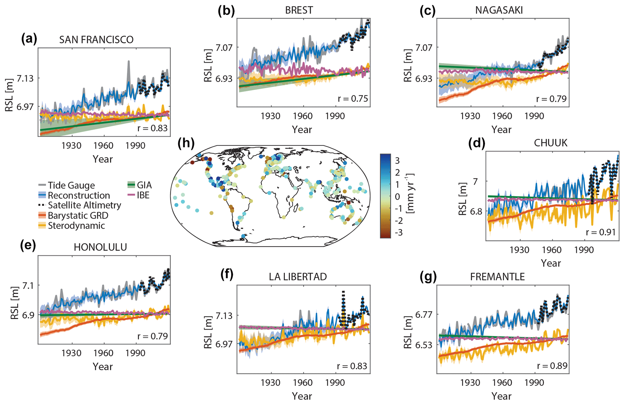
Figure 6 Estimates of relative mean sea level (RSL) and individual contributing factors at tide gauge locations and related biases. Shown are tide gauge and satellite altimetry records (with the GIA added from the reconstruction) at seven selected locations (a–g), together with the new reconstruction and the estimates of individual contributing factors. Uncertainties are shown as shaded regions. Correlations between the reconstruction and the tide gauge records are shown in the lower right of each panel. (h) Differences between the linear trends estimated from tide gauge records and the new reconstruction over the overlapping period between 1900 and 2022.

Figure 6h shows the linear-trend differences between tide gauge records and the nearest-neighbor time series of the weighted fields of the Kalman smoother reconstructions at all 516 sites during the overlapping period at each location. The median difference over all sites is 0.1 mm yr⁻¹, with a standard deviation of 1.8 mm yr⁻¹. This suggests that while there is only a minor systematic bias (0.1 mm yr⁻¹) between tide gauge observations and the reconstruction, there are many sites where the observed trends cannot solely be explained by the sum of individual components. A total of 64 % of all sites show trend differences below 1 mm yr⁻¹, while a trend difference of about 0.5 mm yr⁻¹ or less is observed at 33 % of all sites. The largest and sometimes systematic differences occur in the GIA hotspots of Scandinavia and the North American west coast, in parts of the Gulf of Mexico, and on the Pacific coast of South America. There are several possible explanations for those larger differences. First, our process estimates may have larger uncertainties than implied in the pre-described ensembles, including those resulting from the limitations of 1-dimensional GIA modeling (Thompson et al., 2023). Second, there may be processes that affect tide gauges at the coast (such as nonlinear VLM) but that are not explicitly included as priors in the Kalman smoother fields. While those can, in principle, be captured by the residual term at individual tide gauge sites, they are not part of the global and regional sea-level reconstructions (Hay et al., 2015, 2017).

The good agreement between the reconstruction and both satellite altimetry and steric height at the basin scale, however, suggests that both the sum and individual components are generally well captured by the reconstruction. Indeed, when compared to the 516 tide gauge records over the satellite period from 1993 to 2021, trend differences are on the order of 0.2 ± 2.17 mm yr⁻¹ (median ± standard deviation). The trend differences are −0.06 ± 0.42 mm yr⁻¹ when considering satellite altimetry at the same locations. Thus, there may indeed be other processes, such as residual VLM unrelated to GIA, that are captured by tide gauges but not included within the weighted fields of the Kalman smoother reconstruction. To test this hypothesis, we downloaded GNSS-derived VLM rate estimates provided by SONEL (URL7A from Gravelle et al., 2023), which are available for 601 locations worldwide that provide a minimum observation length of 7 years. Not all GNSS locations align with the tide gauge sites in our assessment. Accordingly, we only consider VLM estimates from locations that have a maximum distance of 8 km (this is the number below which results remain essentially unchanged) to the tide gauge records and where at least 75 % of the period since 1993 is covered by the tide gauge record. This results in 90 sites worldwide. At those 90 locations, we replace the weighted GIA estimate from the Kalman smoother reconstruction by the VLM estimate. To avoid double counting the VLM effects related to contemporary GRD, we remove the linear-rate estimate of its deformational component since 1993 from GNSS estimates. We also add the GIA sea-surface height component from the weighted Kalman smoother GIA fields to the GNSS estimates (Tamisiea, 2011). The trend comparison is performed over the period 1993 to 2021 to ensure that the time window relative to GNSS observations is comparable. The trend differences between observed tide gauge records, the nearby weighted Kalman smoother fields, and the nearby weighted Kalman smoother fields with GNSS-based VLM are shown in Fig. 7 as spatial maps (Fig. 7a and b) and empirical distributions (Fig. 7c). The trend differences for the 90 selected sites, 0.27 ± 1.67 mm yr⁻¹, are not significantly different from those obtained at all 516 sites (0.1 ± 1.8 mm yr⁻¹). However, replacing the GIA crustal rates with the GNSS-based VLM at the 90 sites significantly reduces the trend differences to −0.13 ± 1.00 mm yr⁻¹ (i.e., a reduction of 40 % in the standard error). Applying the same test to the entire period over which tide gauges provide data results in very similar results (a reduction in standard error from 1.5 to 1 mm yr⁻¹ at 119 sites). The reduction is most prominent at the locations of former ice sheets in Scandinavia and North America, but it is also visible at sites that are known to be affected by residual VLM, such as along the Japanese coastline. Thus, some of the observed differences from tide gauge observations are likely related to unaccounted-for VLM (in addition to shorter-term variations; for instance, those associated with near-coastal processes that are captured by neither satellite altimetry nor the reconstruction). This result also indicates that the Kalman smoother framework is robust against potential biases caused by these residual processes. Future work might assess the suitability of the framework for assessing nonlinear VLM at individual tide gauge sites (Kopp et al., 2014; Dangendorf et al., 2021).

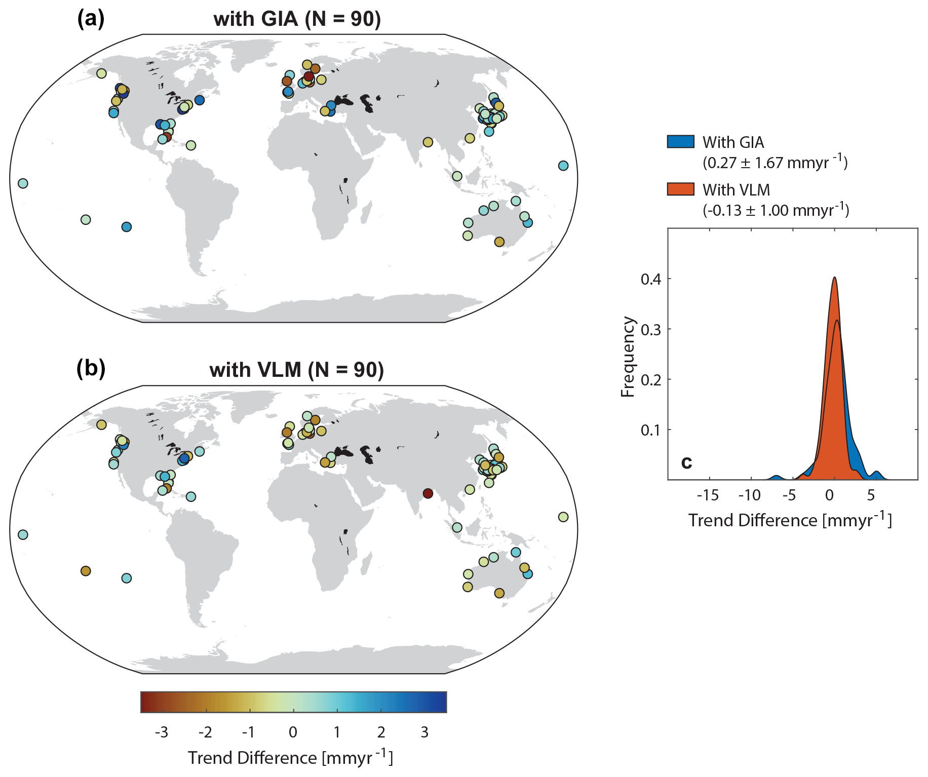
Figure 7 Linear-trend biases at tide gauge sites and the role of VLM. Shown are (a) the linear-trend differences between tide gauge records and the new reconstruction over the overlapping period between 1993 and 2021, which were obtained considering the reconstructed GIA as VLM, and (b) an alternative estimate where the reconstruction is combined with the observed VLM from a GNSS (corrected for the VLM from contemporary GRD and with sea-surface height changes due to GIA added). The corresponding kernal density estimates of trend differences between tide gauge records and the reconstruction over their overlapping period from 1993 to 2021 is shown in (c).

3.2 Trends and variability in GMSL

After demonstrating the performance of the new reconstruction, we now turn our attention to the modeled changes over the 20th century. Again, the respective global and basin-scale time series of sea level and individual contributors are shown in Fig. 3, with their respective linear trends summarized in Table 3. In the new reconstruction, GMSL has been increasing by a linear rate of about 1.5 ± 0.2 mm yr⁻¹ since 1900. This is lower than the 1.7 ± 0.2 mm yr⁻¹ reported by Church and White (2011) and the 2.10 ± 0.3 mm yr⁻¹ reported by Jevrejeva et al. (2014) for the period from 1900 to 2009, but it is consistent with more recent reconstructions that consider the spatial patterns of individual sea-level processes as prior estimates in the reconstruction process (Hay et al., 2015; Dangendorf et al., 2017, 2019; Frederikse et al., 2020).

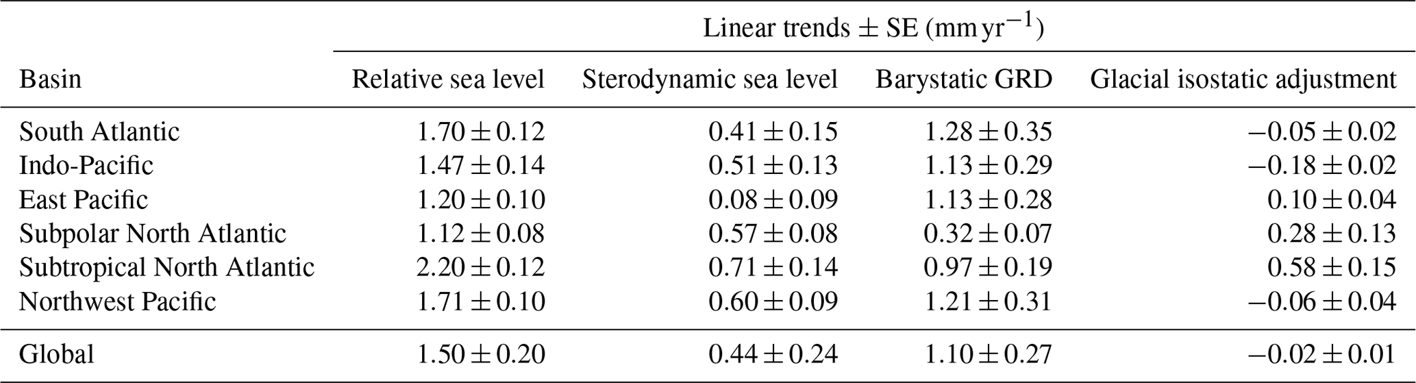
Table 3 Linear trends in global and regional sea levels and individual contributors over 1900 to 2021. All trends have been calculated based on ordinary least-squares regression. Trend uncertainties are presented as standard errors calculated assuming that the residuals are autocorrelated and can be reasonably well approximated by an autoregressive process of order 1. They also contain the reconstruction uncertainty.

It is well known that the reconstructions generally agree well for the 1970s on, while they diverge before that period (Oppenheimer et al., 2019; Palmer et al., 2021). Frederikse et al. (2020) estimated the GMSL but also compared it to the sum of independently measured/modeled contributions. While the long-term trends in both over 1900 to 2018 agreed within their respective uncertainties (1.56 ± 0.2 mm yr⁻¹ for GMSL compared to 1.52 ± 0.2 mm yr⁻¹ for the sum of individual contributions), some differences between both curves appear between the 1920s and early 1950s. All former GMSL reconstructions, including the curve from Frederikse et al. (2020), show enhanced rates peaking in the 1940s and 1950s, while the sum of individual contributions peaks in the 1930s. This is illustrated in Fig. 8b, in which rates of GMSL rise were calculated using a singular spectrum analysis with an embedding dimension of 15 (thereby smoothing the time series to timescales longer than 30 years; Moore et al., 2005); not that the error bars consider the reconstruction uncertainty. Interestingly, in the new reconstruction, rates peak earlier and closely resemble the sum of individual components from Frederikse et al. (2020). We attribute this behavior to the inclusion of barystatic estimates in the new Kalman smoother framework, which changes the regional sea-level fields near major melt sources and then propagates these into the estimation of residual sterodynamic fields. This becomes visible when examining the differences between the regional sea-level rates from this study and those from Dangendorf et al. (2019) over the period from 1930 to 1939 (Fig. 9). Notable differences occur in the vicinities of major melt sources (i.e., Greenland, Svalbard, and Alaska), confirming that the original Kalman smoother framework is not able to properly assign the sea-level signal during this period to its individual barystatic components, given the available number of tide gauges and their locations in the far field of melt sources (Hay et al., 2017). Here, this problem is overcome by pre-describing the melt signals in the initial prior estimates. We also find significant differences in the Pacific region, indicating that the inclusion of the barystatic estimates impacts the estimation of the spatial pattern of sterodynamic sea-level change. In Dangendorf et al. (2019), RSOI was applied to the full sea-level signal and therefore also included potential short-term effects of barystatic GRD processes, while here, RSOI is solely applied to residual signals after accounting for all other budget components.

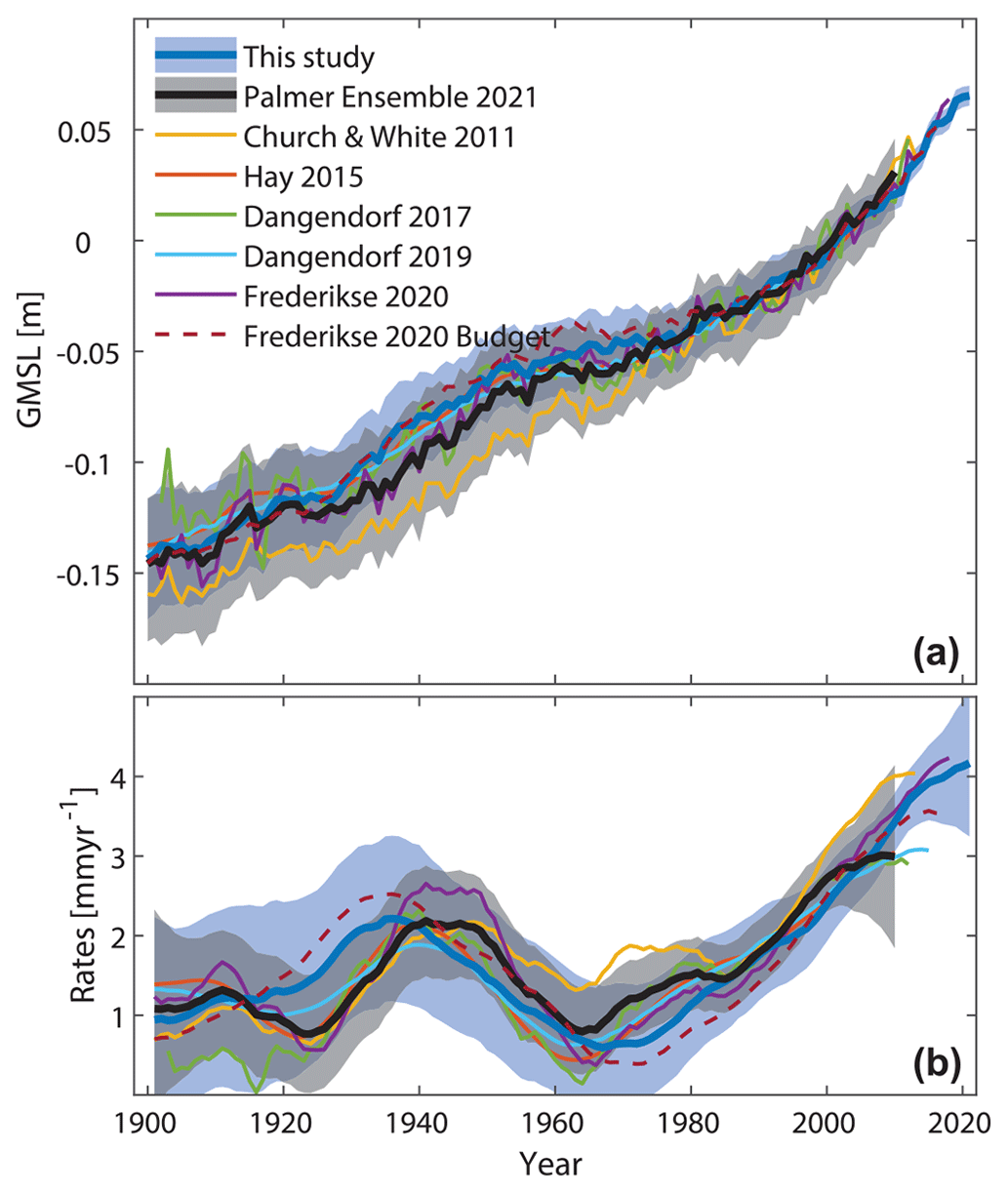
Figure 8 GMSLs and nonlinear rates in comparison to former reconstructions. (a) Shown are the GMSL time series from this study (1900 to 2022) in comparison to selected former reconstructions. All time series have been adjusted to a common mean of zero over the overlapping period from 1993 to 2010. (b) The corresponding nonlinear trends as determined by a singular spectrum analysis with an embedding dimension of 15, which extracts signals that are representative of timescales longer than 30 years. Uncertainties are shown as shaded regions and represent 95 % confidence intervals.

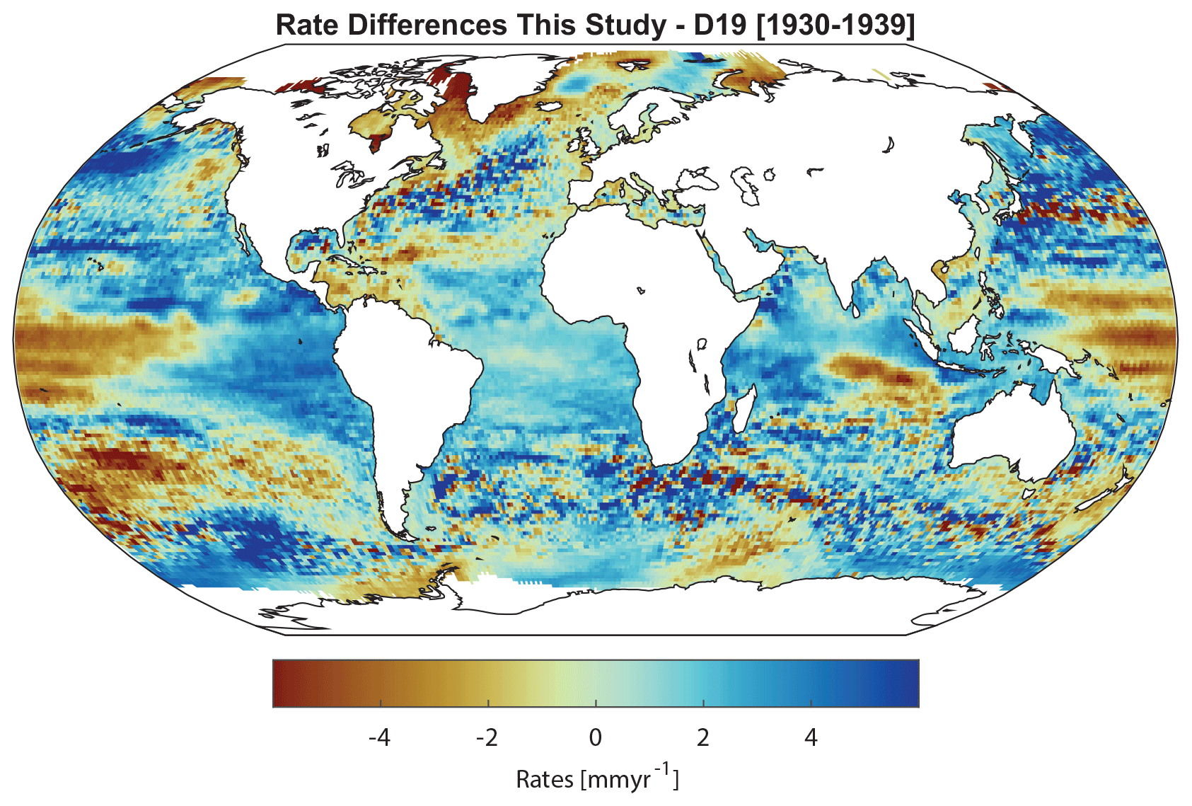
Figure 9 Rate differences between this study and the regional sea-level fields from D19 in Dangendorf et al. (2019) over the period from 1930 to 1939. Differences have been calculated between GIA-corrected fields and thus primarily reflect differences in impact between GRD, the sterodynamic sea level, and IBEs.

We note, however, that the overall evolution of multidecadal rates in GMSL remains generally consistent with moderate rates at the beginning of the 20th century, enhanced rates in the 1930s, a slowdown with a low in the 1960s, and a persistent increase in the rate of rise thereafter (Dangendorf et al., 2019). Consequently, central estimates of multidecadal trends have exceeded 4 mm yr⁻¹ since 2019 for the first time in the observational history, leading to an overall acceleration of about 0.08 ± 0.04 mm yr⁻² since 1970 (Fig. 8b). Over the shorter altimetry period since 1993, acceleration coefficients are slightly larger but consistent within the error, with values of 0.1 ± 0.06 and 0.12 ± 0.1 mm yr⁻² for satellite altimetry and the Kalman smoother reconstruction, respectively.

The steric and barystatic components have contributed about one-third and two-thirds to the increase in GMSL since 1900, respectively (Table 3). For the steric contribution, rates of sea-level rise have been consistently increasing from slightly negative rates in 1900 to rates close to 2 mm yr⁻¹ in 2021 (Fig. 10). The negative rates in the early 20th century are consistent with the steric reconstruction from Zanna et al. (2019) and global atmospheric mean-surface-temperature reconstructions (Lenssen et al., 2019), indicating that both the ocean and the atmosphere were globally in a cooling phase during that period. Barystatic contributions to sea level have been more variable than the steric height, with peak rates occurring in the 1930s (consistent with accelerated warming at high latitudes of the Northern Hemisphere; see Hergerl et al., 2018) and since the early 2000s and near-zero rates occurring in the late 1960s and early 1970s (Fig. 10). This period of low rates has previously been attributed to the increased activity in dam building at that time (Frederikse et al., 2020), which prevented freshwater from flowing into the ocean. The increase in the rate since the early 1970s (which is consistent with former reconstructions summarized in Palmer et al., 2021) was initially driven by the steric contribution and later by the barystatic component of sea-level rise. Overall, barystatic sea-level change is the dominant factor behind the acceleration since 1970 (Fig. 11), although this perspective would change upon considering individual sources of the barystatic sea level (i.e., glaciers, the Greenland ice sheet, the Antarctic ice sheet, and hydrology); in that case, the steric height would be the single most important driver of acceleration since 1970, consistent with Dangendorf et al. (2019).

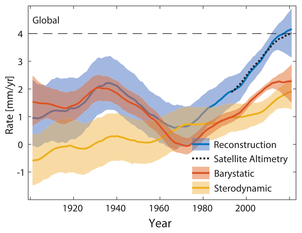
Figure 10 Rates of GMSL rise and its causes. Shown are the nonlinear rates of GMSL rise and its individual contributors as determined from the Kalman smoother framework and satellite altimetry. Rates have been calculated with a singular spectrum analysis using an embedding dimension of 15 (equal to a cutoff period of 30 years).

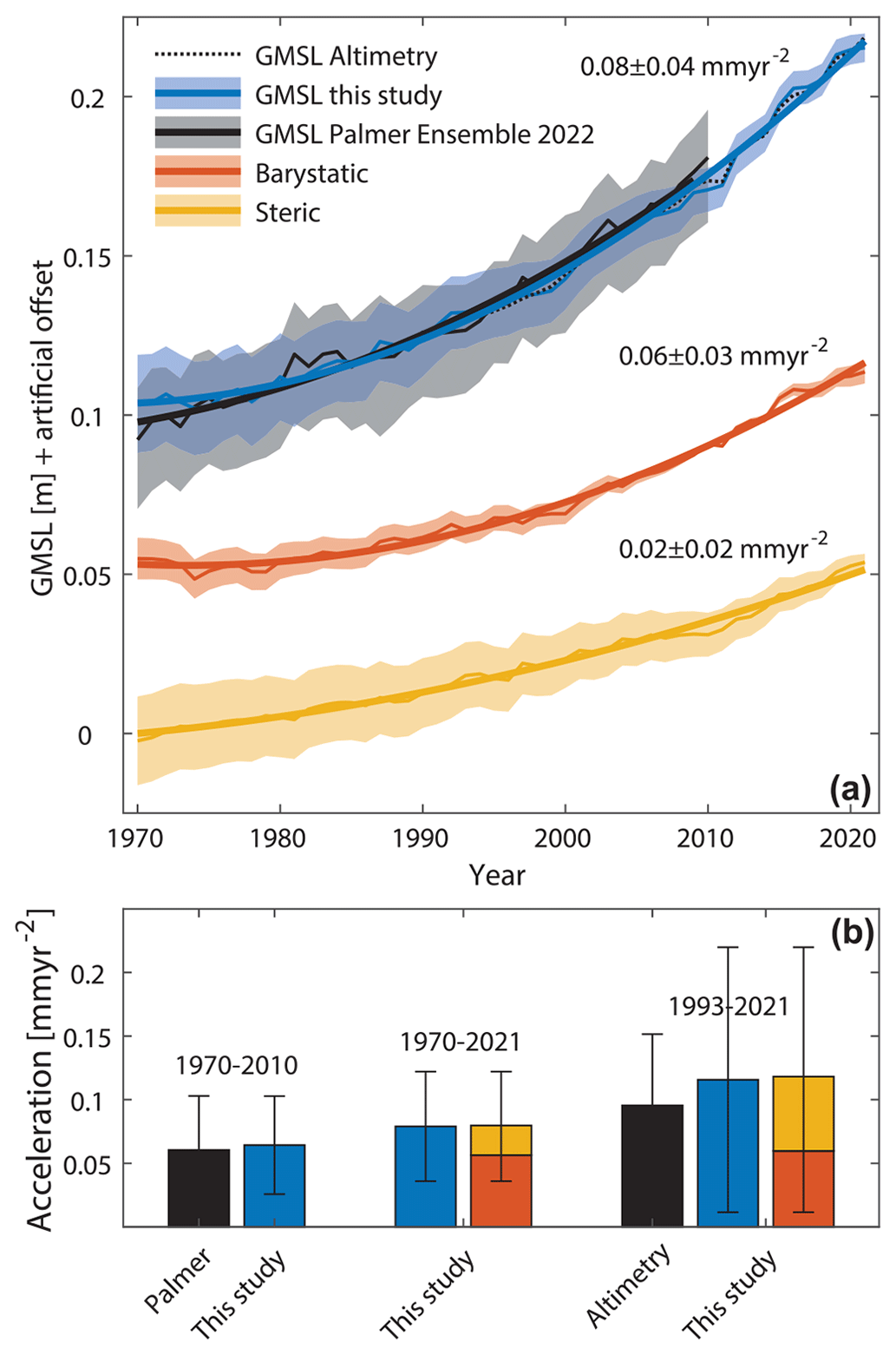
Figure 11 GMSL acceleration since 1970 and individual contributors. (a) Time series of GMSL and the steric and barystatic contributions to it since 1970. Also shown for comparison is the GMSL ensemble estimate based on previous reconstructions, as assembled by Palmer et al. (2021). Thin lines show the annual reconstructions, thick lines represent a quadratic fit. (b) Quadratic coefficients estimated over different periods and using different individual contributors.

3.3 Trends and variability in regional sea level

At the basin scale, the trends as well as the relative contributions of individual components can vary significantly (Table 3). Most notably, in the subtropical North Atlantic, relative sea level has increased 146 % faster than GMSL, leading to rates of about 2.2 ± 0.12 mm yr⁻¹. While barystatic GRD contributions have been slightly below the global average due to their proximity to Northern Hemispheric melt sources, sterodynamic and GIA contributions have been rising at faster rates than anywhere else. This is qualitatively consistent with the results from Frederikse et al. (2020) for the shorter period since 1958 and reflects, in terms of the sterodynamic component, the above-average increase in ocean heat content in the Subtropical Gyre (Cheng et al., 2022). The lowest trends over the 20th century occurred in the subpolar North Atlantic, with rates of about 1.12 ± 0.08 mm yr⁻¹. These lower trends are foremost a result of the reduced contributions of barystatic GRD, which has been increasing at a pace 71 % less than the global mean (0.32 ± 0.07 mm yr⁻¹ compared to 1.1 ± 0.27 mm yr⁻¹).

An important feature of the new reconstruction is that it provides not only global and basin-scale estimates but also local sea-level changes, including estimates of the individual contributors (Fig. 6). This is a major advance relative to earlier studies, particularly with respect to the representation of dynamic redistribution processes within the sterodynamic component. Previous studies of sea-level budgets based on conventional steric height products from temperature and salinity profiles pointed to the difficulty of properly estimating the manometric sea-level contribution in the coastal zone (Cabanes et al., 2001; Miller and Douglas, 2004; Frederikse et al., 2018; Dangendorf et al., 2021). In contrast, here, the sterodynamic signal is entirely determined by coastal signals as measured by tide gauges. This enables us to perform more sophisticated analyses of past trends and accelerations at a global level, with a focus on individual budget contributions.

Figure 12 shows linear trend maps for relative sea level and individual sterodynamic, barystatic GRD, GIA, and IBE contributions since 1900, including 5° latitudinal averages of the corresponding trends. Linear trends in the reconstruction range from −4.2 to 11.7 mm yr⁻¹ for relative sea levels (Fig. 12a). Negative trends are primarily located in centers of postglacial uplift where former ice sheets were located (Scandinavia and North America) and are therefore caused by the GIA signal and, to lesser extent, GRD in response to modern melting (Fig. 12d). The largest positive trends appear in eddy-rich regions near western boundary currents such as the Kuroshio, the Gulf Stream, and the Agulhas system and are related to changes in ocean circulation (i.e., the sterodynamic component; Fig. 12b). Those changes are more localized and can reverse sign over a few hundreds of kilometers, and they are generally very uncertain due to the paucity of tide gauge records in those regions. Larger geographical areas characterized by strong positive trends are also found along the US East and Northwest coasts; in both cases, this is related to GIA and, specifically, the postglacial subsidence of peripheral bulges (Fig. 12d). There is also a strong trend gradient in sea level across the central Pacific (negative to neutral trends in the east; strong positive trends in the west that also persist into portions of the Indian Ocean), possibly caused by wind-driven (Merrifield, 2011) and buoyancy-driven (Piecuch and Ponte, 2012) sterodynamic processes linked to Pacific decadal climate variability (Fig. 12b). For instance, the Southern Oscillation Index, which measures sea-level pressure differences between Darwin and Tahiti, indicates a weakening over the 20th century (Power and Kociuba, 2011). Similarly visible is the meridional gradient in the South Pacific, discussed in greater detail, albeit for shorter time periods, in Volkov et al. (2017) and Dangendorf et al. (2019). Both studies found a link between sea level in this region and wind-forcing-linked changes in the intensity and position of Southern Hemispheric westerlies. However, more research is warranted to clarify the role of these processes on a centennial timescale, as represented here by the linear trends. Barystatic GRD trends are spatially smoother (Fig. 12c), with strong spatial gradients occurring only in the vicinity of major 20th-century melt sources. Latitudinal averages (Fig. 12a) indicate a general tendency towards larger trends in lower latitudes, with local maxima around ∼40° north and south. This pattern is largely dominated by the barystatic GRD terms and results from the fact that most major melt sources in the 20th century were in high (northern) latitudes. The local maxima around ∼40° north and south are due to the sterodynamic contribution and reflect gyre dynamics. IBE contributions are minor everywhere except at latitudes south of 50° S, where trends of up to 0.8 mm yr⁻¹ are visible. These trends stem from atmospheric pressure changes linked to a hemispheric-scale intensification and poleward shift of the westerlies in this area (Swart et al., 2015), although we caution that the IBE is based on only one atmospheric-reanalysis dataset here. Atmospheric reanalyses are generally known for their uncertainty in this region (Piecuch et al., 2016).

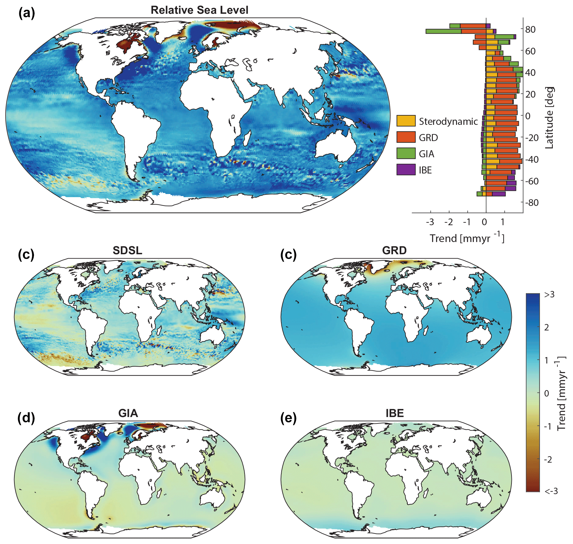
Figure 12 Linear trends in reconstructed sea level and the individual contributing factors over 1900 to 2021. Shown are the linear-trend maps for relative sea level (a), sterodynamic sea level (b), the effects of gravitation, rotation, and deformation (GRD; c), glacial isostatic adjustment (GIA; d), and inverse barometer effects (IBEs; e). In (a), linear trends are presented for all contributors averaged over 5° latitude bands.

Next, we turn our attention to the spatial acceleration pattern since 1970 (Fig. 13). The choice of this period is based on the persistent acceleration visible in the GMSL rise since 1970 (Fig. 11). There is large spatial variability in acceleration coefficients, which range from negative values (i.e., deceleration) as low as −0.8 mm yr⁻² to positive accelerations as large as 1.17 mm yr⁻². Thus, even over this 52-year period since 1970, the regional acceleration coefficients can vary by an order of magnitude relative to the global mean value (0.08 mm yr⁻²). This indicates that acceleration coefficients are very sensitive to regional redistribution processes and natural climate variability, hampering the robust and timely detection of more-persistent forced long-term signals (Haigh et al., 2014; Dangendorf et al., 2014a, b; Hamlington et al., 2022). Decelerations in the rate of sea-level rise primarily occur as a result of barystatic GRD effects in the vicinity of major melt sources, particularly around Greenland (Fig. 13a and c). There is also one larger spot of pronounced deceleration coefficients in the South Pacific Ocean south of 50° S. Previous studies have indicated that this deceleration is related to an increased amplitude and localized northward shift of Southern Hemispheric westerlies in the South Pacific (Volkov et al., 2017; Dangendorf et al., 2019). As a result, upper-ocean warm water has moved northwestward, leading to a deceleration of the sterodynamic signal southward (Fig. 13b) and, at the same time, the initiation of an acceleration hotspot in the central subtropical South Pacific. Note that IBE contributions have slightly compensated for these sterodynamic effects due to changes in sea-level pressure (Fig. 13e). The acceleration in the tropical South Pacific further extends into both the equatorial western Pacific and large parts of the tropical Indian Ocean, making it the largest continuous area affected by accelerating sea levels over this period worldwide. This trend is also supported by the latitudinal averages in Fig. 13a, thus bolstering results from earlier studies based on different techniques (Merrifield et al., 2009) or earlier versions of the Kalman smoother that used different priors (Dangendorf et al., 2019), which indicated an important role of tropical regions and the Southern Hemisphere in driving the recent acceleration in GMSL. Again, barystatic GRD effects (Fig. 13c) are spatially smoother than their sterodynamic counterparts (Fig. 13b), and they contribute coherently positively to the acceleration, making them the most dominant contribution to latitudinal averages south of 30° N (Fig. 13a).

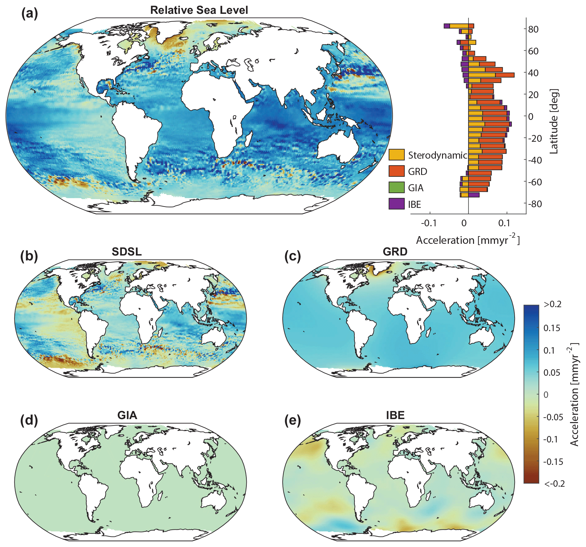
Figure 13 Acceleration coefficients for reconstructed sea level and the individual contributing factors over 1970 to 2021. Shown are the acceleration coefficient maps for relative sea level (a), sterodynamic sea level (b), the effects of gravitation, rotation, and deformation (GRD; c), glacial isostatic adjustment (GIA; d), and inverse barometer effects (IBEs; e). In (a), acceleration coefficients are presented for all contributors averaged over 5° latitude bands.

To better place some of the observed decelerations and accelerations into a historical context, we select five case-study sites in areas of strong deceleration or acceleration (the purple boxes in Fig. 14a). Around Greenland, relative sea levels have been alternating around zero since 1900, with positive rates peaking in the 1920s and late 1980s and negative lows in the 1930s and the 2010s (Fig. 14b). The transition from increasing rates in the 1970s and 1980s to negative rates in the 2000s has led to a deceleration in this area, which is largely driven by barystatic GRD effects (Coulsen et al., 2022). However, we note that the low rates in the 2000s are still slightly higher than the lows in the 1930s and are thus not unprecedented. Sterodynamic sea level has risen steadily in this area, with an average rate of ∼0.6 mm yr⁻¹, which is qualitatively consistent with Spada et al. (2014). The largest uncertainties in the total rates are related to the GIA contributions, likely due to ice histories and assumptions made about the Earth's rheology in modeling (Spada et al., 2014). In the South Pacific, sea levels have been decelerating over this period as well (Fig. 14c), but the decomposition into individual components is very different compared to the Greenland example. Here, the sterodynamic component has been the dominant source of multidecadal variability in the rates. Over the entire period, sterodynamic sea level has been decreasing by an average rate of ∼1 mm yr⁻¹. Minima in the signal occurred in the 1940s and the late 2000s, but they have been partially counterbalanced by barystatic GRD and IBE contributions. In the Gulf Stream (Fig. 14d) and Kuroshio (Fig. 14e) regions, rates have been rising faster than elsewhere, with average rates of approximately 2.7 and 1.9 mm yr⁻¹, respectively. This rise is clearly dominated by sterodynamic contributions. In the larger Kuroshio region (Fig. 14e), rates have consistently increased from 1 mm yr⁻¹ in 1980 to 5.8 mm yr⁻¹ in the most recent years, while the increase began later (in the late 1990s) in the larger Gulf Stream region, with the rate rising from 3.1 mm yr⁻¹ in 1999 to 7 mm yr⁻¹ in 2021. In both regions, accelerations have also been reported along the adjacent coastlines of Japan (Usui and Ogawa, 2022) and the Southeast of the United States (Dangendorf et al., 2023; Yin, 2023; Steinberg et al., 2024), with rates exceeding 10 mm yr⁻¹ locally. In both regions, sterodynamic variability has been the most dominant contributor to variations in the rates, while barystatic GRD contributed a smoother but consistently positive signal over most of the 20th century. Due to the geographic proximity to the Laurentide ice sheet, GIA adds more uncertainty to the total rates of relative sea-level rise in the Gulf Stream region than to those in the Kuroshio region (Fig. 14d and e). In the tropical western Pacific, sea levels have also been rising faster (2 mm yr⁻¹) than the GMSL (1.6 mm yr⁻¹) (Fig. 14f). High rates (close to 5 mm yr⁻¹) occurred in the early 1900s and the late 1990s. Both peaks were dominated by the sterodynamic component and were coeval with minima in the Southern Oscillation Index (representing sea-level pressure differences between Tahiti and Darwin). While sterodynamic rates slightly decreased after the peak in 1999, rates of relative sea-level rise plateaued due to increasing contributions from barystatic GRD. Both the GIA and IBE contributions play a minor role in these areas. In general, we find that the sterodynamic contribution mostly dominates nonlinear rates locally at timescales of up to a few decades, while the barystatic contribution becomes more important at larger spatial and temporal scales.

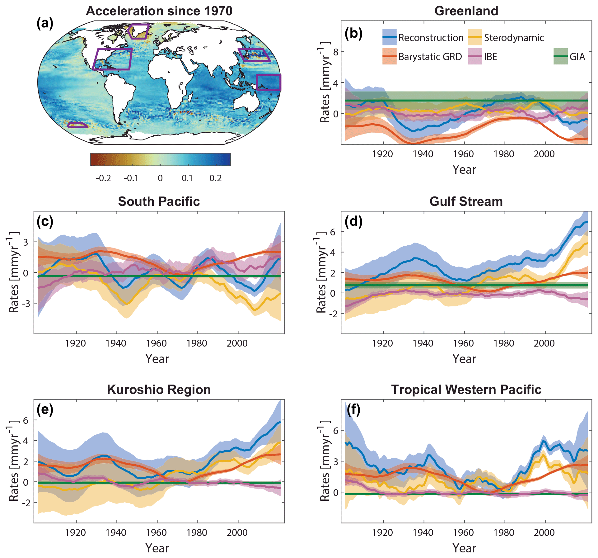
Figure 14 Acceleration since 1970 and nonlinear rates in selected hotspot regions around the world. (a) Map of acceleration coefficients determined over the period from 1970 to 2022 (the same as for Fig. 6) together with selected areas (purple boxes) for which the average rates of sea-level rise are shown in (b–f). Rates of nonlinear relative sea-level rise and individual contributing factors as determined by the new reconstruction are shown for Greenland (b), the South Pacific (c), the Gulf Stream Extension region (d), the Kuroshio Extension region (e), and the tropical western Pacific (f). Nonlinear rates were determined with a singular spectrum analysis with an embedding dimension of 15, producing trends that are representative for timescales longer than 30 years. Uncertainties are shown as shaded regions and represent 95 % confidence intervals.

Overall, these results underscore the importance of embedding recent accelerations into a historical context. The new Kalman smoother reconstruction provides interesting new insights into the causes of sea-level changes at a near-global coverage that complements tide gauge and satellite observations and can motivate more detailed assessments in case-study regions that are beyond the scope of this study.

4 Code and data availability

We provide access to the full sea-level reconstruction, including all contributing processes and related uncertainties. The data are archived as MATLAB and netcdf files and can be accessed via Zenodo at the following link: https://doi.org/10.5281/zenodo.10621070 (Dangendorf, 2024). Data are provided as a spatiotemporal field for each individual component with 74 742 grid points, a separate uncertainty field, and the associated global- and basin-scale averages and their related uncertainties. Codes for the analysis of the sea-level fields and the production of the figures are also provided. The code for the Kalman smoother reconstruction is currently still being prepared for publication but is available from the main author upon request. We intend full publication of the Kalman smoother approach with the next version of the reconstruction in a future release with cleaned-up and annotated codes.

5 Discussion and conclusions

Here, we have introduced a new Kalman-smoother-based estimate of global and regional sea-level changes and their causes over the period from 1900 to 2021. Innovations compared to earlier versions (Hay et al., 2015; Dangendorf et al., 2019) are our adoption of adjusted estimates of GIA, observation-based and reconstructed barystatic GRD (as a combination of the contributions from glaciers, ice sheets, hydrology, and terrestrial water sources), IBE contributions, and (reconstructed) sterodynamic variability. As a result, the new reconstruction moves beyond global and regional sea-level estimates to resolve the individual contributing processes locally over the entire 20th and early 21st centuries.

The new reconstruction provides 6 more years of data than our earlier works using different techniques (Dangendorf et al., 2019; the RSOI approach was used in that study as a post-processing step at timescales smaller than 30 years, while RSOI is integrated directly into the Kalman smoother framework for the reconstruction of the sterodynamic sea level here). The reconstruction shows excellent agreement with satellite altimetry in terms of variability (median r∼0.86 over all the oceans), trends (median differences of 0.02 ± 0.42 mm yr⁻¹), and accelerations (median differences of −0.01 ± 0.13 mm yr⁻²) over their overlapping period from 1993 to 2021. We also find moderate to good agreement between the reconstructed sterodynamic sea level and independent steric-height estimates from temperature and salinity fields in terms of correlation, but we note that three out of six ocean basins show trends that are larger than those in steric-height fields. Compared to tide gauge records extending back to the early 20th century, reconstruction at a nearby site utilizing a sum of the barystatic GRD, sterodynamic sea level, IBEs, and GIA often underestimates the absolute trends. However, we demonstrate that for 90 sites equipped with a nearby GNSS, the resulting trend error can be reduced by ∼40 % when the VLM from the GNSS is considered in the comparison. This indicates that unaccounted-for residual VLM that is induced, for instance, by fluid withdrawals or tectonics (Shirzaei et al., 2021) and has not been explicitly included as a prior is a significant driver of these differences. It also indicates that the Kalman smoother framework is robust against such local processes.

Over 1900 to 2021, our GMSL record shows a long-term trend of about 1.5 mm yr⁻¹, a value that is consistent with the central estimate provided by the Intergovernmental Panel on Climate Change 6th Assessment Report (Oppenheimer et al., 2019; Fox-Kemper et al., 2021). The barystatic sea level and steric expansion have contributed approximately two-thirds and one-third to this increase, respectively. Multidecadal nonlinear trends in GMSL rise indicate four phases of varying rates: moderate rates in the early 20th century (∼1 mm yr⁻¹), enhanced rates at the end of the 1930s and the beginning of the 1940s (∼2 mm yr⁻¹), reduced rates in the 1960s (∼0.5 mm yr⁻¹), and a persistent acceleration thereafter. While this pattern generally agrees with previous estimates of GMSL change (Church and White, 2011; Hay et al., 2015; Dangendorf et al., 2017, 2019; Frederikse et al., 2020; Palmer et al., 2021), the peak in the late 1930s occurs almost a decade earlier than in other reconstructions. This earlier occurrence is more consistent with the sum of individual components from Frederikse et al. (2020) and is primarily the result of considering pre-described barystatic GRD estimates in the Kalman smoother. More research is needed to clarify the extent to which uncertainties in the barystatic GRD estimates (Malles and Marzeion, 2021) may affect the budget and the Kalman smoother estimates of total GMSL change. The persistent acceleration after the low rates in the 1960s has led to central estimates of nonlinear rates since 2019 that, for the first time, exceed 4 mm yr⁻¹ on a multidecadal timescale (Fig. 10). The exceedance of this 4 mm yr⁻¹ level may mark an important threshold change. For instance, it has recently been reported that a widespread retreat of coastal habitats such as tidal marshes and mangroves is likely under sustained sea-level rise rates of 4 mm yr⁻¹ (Saintilan et al., 2023). The fact that the GMSL has now exceeded that threshold means that a large portion of the ocean is already being impacted by those rates. While the acceleration was initiated by steric expansion in the 1960s and early 1970s, it has been the mass loss from glaciers and ice sheets that has dominated the acceleration over the last few decades. Spatially, the highest coastal trends since 1900 have occurred in the vicinity of western boundary currents and tropical regions. Since 1970, the acceleration has been highest in the Kuroshio region, the subtropical North Atlantic (Dangendorf et al., 2023; Yin et al., 2023), and (sub)tropical regions of the Indo-Pacific, consistent with earlier studies (Merrifield et al., 2009; Dangendorf et al., 2019). In contrast to the GMSL, the varying rates of sea-level rise in those regions have been dominated by sterodynamic processes at timescales of ∼30 years. This reinforces our conclusion that improving the understanding and prediction of local sea levels at decadal timescales requires a fundamentally deeper understanding of sterodynamic variability (Dangendorf et al., 2021).

Our new reconstruction may be relevant for several applications. First, it extends the satellite record back to 1900, adding more than 4 times the original data. Thus, the reconstruction can be used to better characterize natural variability in local sea levels and provide more robust detection of emerging trends and accelerations from the satellite record. Trend and acceleration detection techniques have recently been used for making decadal predictions and trajectories (Hamlington et al., 2022; Sweet et al., 2022) as a decision-making support tool in the realm of dynamic-adaptation pathways (Haasnoot et al., 2013). The new reconstruction also provides important information on sea level and its contributing factors in otherwise data-sparse regions such as South Asia and Africa (Woodworth et al., 2010), complementing the sparse tide gauge records that exist and serving as a benchmark for datum homogenization procedures for uncertain observations (Hogarth et al., 2020). The reconstruction can also be used as a boundary condition for global (Muis et al., 2020) and regional storm tide modeling (e.g., Arns et al., 2015) to incorporate possible dependencies and changes through time or to serve as a basis for high-resolution sea-level reconstructions for impact assessments (Treu et al., 2024). Last, we note that an earlier version of our reconstruction (Dangendorf et al., 2019) was partially based on the use of historical climate model outputs as priors. This prevented the IPCC from more detailed comparisons with climate model outputs over the historical period in addition to tide gauges (Oppenheimer et al., 2019; Fox-Kemper et al., 2021). The new reconstruction is entirely based on observational products and is thus independent of climate model simulations. Thus, more detailed comparisons as well as detection and attribution assessments are now possible.