the Creative Commons Attribution 4.0 License.
the Creative Commons Attribution 4.0 License.
 | 20 Nov 2026
The ICOS Ecosystem Station Loobos: a pine forest site exposed to atmospheric pollution
Michiel K. van der Molen

Henk Snellen
Rupert Holzinger
Johannes G. M. Barten
Hong Zhao
Laurens Ganzeveld
Julie Fry
Wouter Peters
Maarten Krol
Jordi Vila-Guerau de Arrellano
Bart Kruijt
The Loobos Ecosystem Station (ICOS: NL-Loo) is in a pine forest on sandy soil, the most dominant forest type in the Netherlands. The station was first built in 1995 and the first atmospheric flux measurements were taken in 1997. The station was one of the first in EuroFlux and FLUXNET. Between 2021 and 2023, the station was rebuilt to meet the ICOS standards as an Ecosystem Class 2 station. The initial purpose of the station was to measure fluxes of heat, water and carbon dioxide. Over time, interest has increased in better understanding the forest water use and ecosystem dynamics and its interaction with air quality. This has resulted in additional concentration and flux measurements of ozone and volatile organic compounds. In the near future, we intend to include measurements of nitrogen species (ammonia and nitrogen oxides) to exploit Loobos' unique location downwind of major anthropogenic emission hotspots. Documenting the instrumentation and exploring the quality of the data is important to understand the observational data. This paper therefore describes the station in terms of geography, ecosystem and instrumentation. DOIs to all described data are provided in the data availability section.
- Article
(17692 KB) - Full-text XML
-
Supplement
(970 KB) - BibTeX
- EndNote


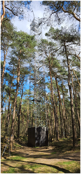
The Loobos station (52.166581° N, 5.743556° E, 24 m above mean sea level) is in a pine forest in the Veluwe area, the largest nature area in the Netherlands, where pine is the most dominant species. In 1995, a first tower was built in Loobos to measure water and carbon dioxide fluxes (Dolman et al., 1998; Zhao et al., 2026). As such, it was one of the 17 first FLUXNET stations globally (FLUXNET, 2010), providing a 25-years (1996–2021) observational dataset of meteorology, turbulent fluxes and net ecosystem exchange at the forest (Zhao et al., 2026). In 2018 a grant from the Dutch Science Fund (Ruisdael Observatory, 2026; NWO, 2026a) allowed the station to be rebuilt with modern instrumentation in a taller tower according to ICOS instructions (Sabbatini and Papale, 2017; Rebman et al., 2018). This second tower was built in March 2021 in the form of a robust 36 m tall scaffolding tower, accessible with stairs, and it was equipped in subsequent months. The main changes required for ICOS labelling include a taller tower, a change from open path to enclosed path CO2 and H2O sensor in the eddy covariance setup, a CO2 profile with many more levels and more extensive ecosystem characterisation. In May 2023, the station was officially labelled as one of 40 ICOS (Integrated Carbon Observing System, ICOS Carbon Portal, 2026) ecosystem stations. Documenting measurement stations is important for understanding and interpreting the resulting data. Therefore, this paper describes the geographic history of the site, its ecosystem and the new station's current and planned extension of instrumentation. We focus on long-term continuous and recurring measurements, and briefly mention experimental campaigns. We demonstrate our capability to measure diurnal cycles of CO2 exchange with eddy covariance and a profile system at the station. This paper describes the instrumentation of the second tower. The first tower's instrumentation is described in Zhao et al. (2026).
1.1 Geographic history
In Pleistocene times, before the last ice ages (> 238 kyr before present, BP), the Dutch landscape was formed by riverine deposits of sand, gravel and clay, hundreds of meters thick, by the rivers Rhine, Meuse and a few smaller rivers from Germany. In the pre-last ice age, the Saalian, 238–126 kyr BP, the northern part of the Netherlands was covered by ice sheets, which formed glacier tongues towards the South (Berg and Beets, 1987; van der Wateren, 1995; Benneth, 2001). Two glacier tongues formed in the (then) Rhine and Meuse river valley, which are the current IJssel valley and Eem valley. The maximum extension of the glacier tongues occurred around 150 kyr BP. The weight of the ice tongues, which were hundreds of meters thick, pushed up the parent material into push moraines, creating the distinct Veluwe massive topography visible in Fig. 1. The sideway motion caused the originally horizontal layers of riverine deposits to be pushed up diagonally, while smearing clay layers, thus creating (semi)impermeable layers (aquitards) (Bakker and van der Meer, 2023). Boulder loam/glacial till was left behind by the glaciers in the valleys.
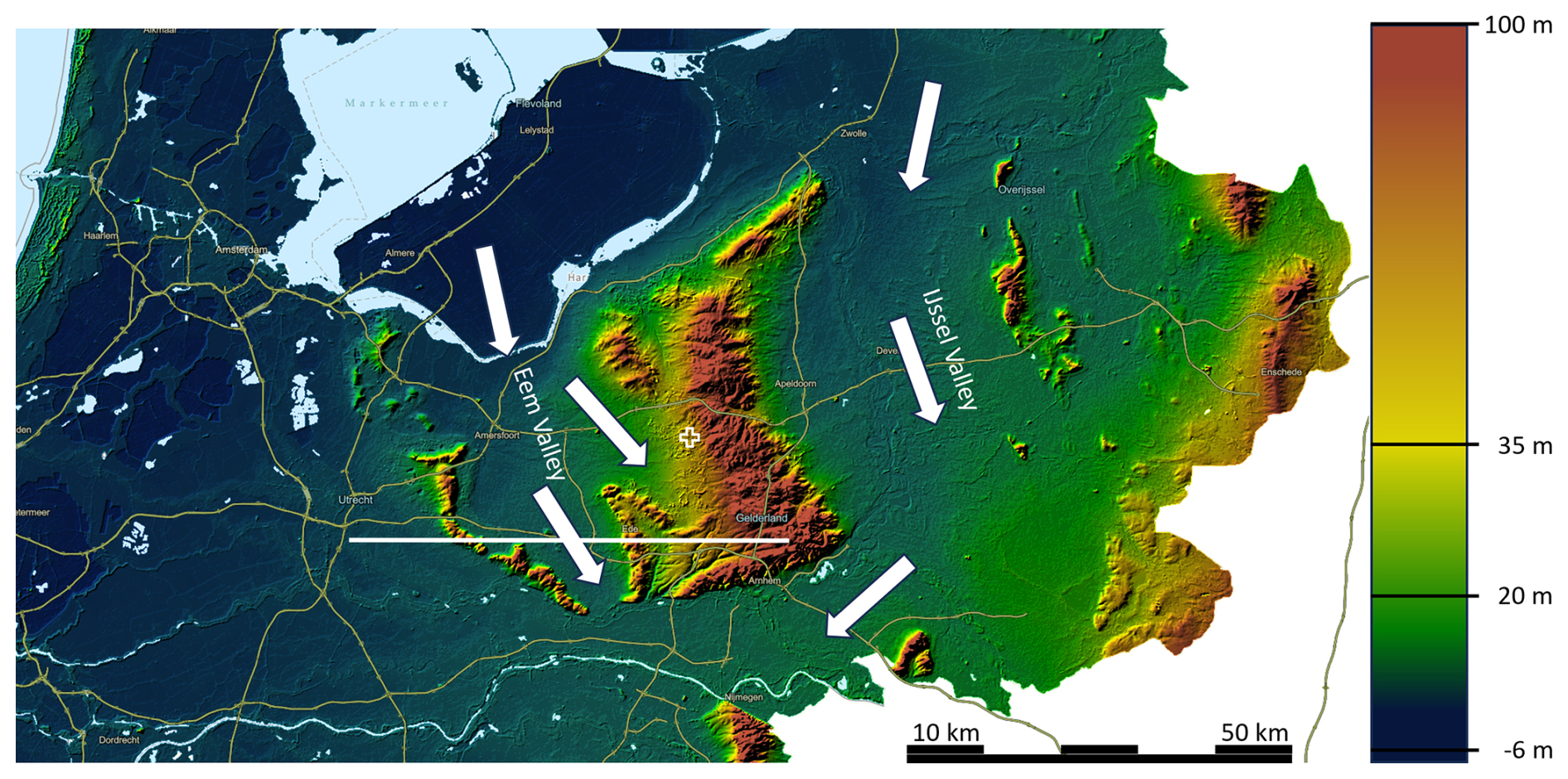
Figure 1General topography of the center of the Netherlands, with the Veluwe massive in the center as a remnant of the push moraines of the Saalian ice wedges in the Eem Valley and the IJssel valley. White arrows indicate the direction of the ice wedges. The + mark indicates the location of the station (Source: Esri Nederland, AHN | Powered by ESRI, https://apps.arcgisonline.nl/hoogteviewer/AHN4/DTM/hillshade, last access: 13 October 2026, kleur/@191242.7204296306,457399.1388867902,3 annotated by authors).
In the Saalian and during the transition to the Eemian interglacial period (126–116 kyr BP), the glacier tongues melted, eroding much of the push moraines, while creating meltwater brooks and Sandr plains (Fig. 2) (see also Fig. 2 in Ruegg, 1983).
In the subsequent last ice age (Weichselian, 116–11.7 kyr BP), the Scandinavian ice sheets did not reach Netherlands. However, in the governing steppe climate, the landscape developed to a polar desert. The sea level was low and the prevailing Westerly winds deposited 15–30 m of wind-blown fine sand from the dry North Sea basin (Data and Information on the Dutch Subsurface, 2026). The Veluwe push moraine was a barrier, and the majority of the sand was thus deposited in the Eem Valley and on the Western flanks of the Veluwe massive.
In the Holocene, (starting 11.7 kyr BP), the climate became warmer. The loam deposits in the former glacier valleys caused those areas to be poorly drained and peat formation occurred. On the push moraines, the diagonally tilted clay layers still slow down the outflow of ground water towards the sides, causing the main direction of ground water flow to be South to North, thus preventing fast discharge and maintaining higher ground water tables than without. The push moraines were covered by dense forests.
For long, the Veluwe area remained forested, but starting early in the Middle Ages (ca. 700 AD), the forest was gradually cut for the iron industry and iron- and coppice coal production (Spek and Kleine Koerkamp, 2022), agriculture, and later for wood production for building construction and commercial and military shipping. The poor soil (“Veluwe”, in old Dutch “Vale Ouwe” is Germanic for “fallow lands”) was, however, not very useful for agriculture, so farmers herded sheep to graze on the heather fields and collected the dung in stables where the sheep remained overnight (pot stall system). Overgrazing caused bare soil to be exposed and wind erosion to occur on large scale.
The wind erosion started from the Western flanks of the Veluwe massive (East of the current N310 road shown in Fig. 2). The peat area further West was too wet. On the East side of the N310 road, sand dunes formed (Fig. 2), which increase in height towards the East. At the location of the station, the dunes are 2 to 10 m tall. The sand dunes were most likely deposited on top of former agricultural lands. Some soil cores taken in the soil campaign (Sect. 2.8.3) suggest evidence for this.
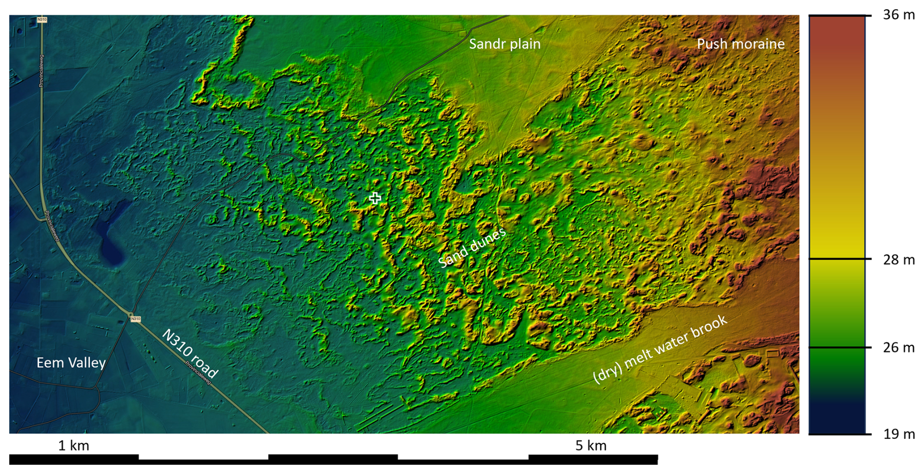
Figure 2Zoom in on the immediate area around the Loobos station. The increasing height of the sand dunes towards the East of the N310 road is clearly visible. (Source: ESRI Nederland, AHN | Powered by Esri, https://apps.arcgisonline.nl/hoogteviewer/AHN4/DTM/hillshade, last access: 13 October 2026, kleur/@180225.44839508645,463590.4012693153,8 annotated by authors). The plus mark indicates the location of the station.
For centuries, citizens and governments fought the wind erosion and sandstorms, unsuccessfully (Witte, 2016). Finally, starting in 1906, the area was planted with predominantly pine trees, starting along the N310 road and moving towards the East. The patch where the Loobos tower is located was planted in 1911 (Topo Time Travel, Kadaster, 2026).
As a result of the (pre-)historic developments, the area has a wind-blown fine sandy soil. The soil was purely mineral before the trees were planted, hence very poor in nutrients. The trees were planted with a turf of peat, but according to conversations with local people, these trees grew very little until after WWII. On multi-annual timescales, the water table currently varies between 2.5 and 4.5 m below the surface in the valleys between the dunes. It is likely that during the young phase, the water tables were closer to the surface, because large-scale drainage systems were not yet installed to facilitate farming in the Eem Valley. From the 1950's onward, when livestock farming became more intensive, NH3 emission from the Eem Valley caused deposition in the forest. CLO (2026) provided estimates that the country average deposition rates peaked at 38 kg N ha−1 yr−1 (24 kg N-NHy and 14 kg N-NOx) in the 1990's and decreased afterwards to 21 kg N ha−1 yr−1 (15.4 kgN-NHy and 5.6 kg N-NOx) in 2023. Regionally, e.g. in the former Eem Valley, deposition rates may be more than double this rate. Melman et al. (2025) estimate the ammonia deposition at 11.6 kg N-NH3 ha−1 yr−1 at Speuld in 2010, a nearby experimental site, which is somewhat less exposed to agricultural deposition than Loobos. Melman et al. (2026), using an open-path ammonia sensor in eddy covariance mode at Loobos, measured a NH3 deposition of 33.3 ± 4.7 kgN ha−1 yr−1. Such deposition rates are among the highest in Europe, and signify substantial acidification of the forest soil (de Vries and Du, 2024).
The continuous high nitrogen deposition and input of acidity may cause microbes and fungi to only slowly decompose the deposited pine needles. As a result, a 5–25 cm thick organic layer has formed on top of the mineral soil. In the 2024 soil campaign, we found very few macro-organisms in the soil, no worms. The soil is classified as Podzol according to the international classification of Mantel et al. (2023).
A tree core campaign in 2010 showed that the trees, whose core had been reached, then had 67 to 97 rings (86 on average). Ring widths grew by about 1.25 mm yr−1 until the early 1960's. After then, the growth rate was variable between 1 and 3 mm yr−1, with maxima in the mid 1960's, mid 1970's and late 1980's and an average of 2 mm yr−1. From about the year 2000, the area was invaded by Prunus serotina, an exotic broadleaf shrub species. The deposited leaves decompose slowly, because of the absence of endemic species feeding on them.
Despite the accumulation of organic material, the ecosystem respiration seems to decrease over time, while one would expect it to increase with more organic matter present. This could be caused by the increasing acidity over time and associated reduced microbial activity.
This historical and geomorphological perspective explains how the pine forest now grows on originally nutrient poor fine sandy soil which has developed to a Podzol (Fig. 3) under influence of poorly decomposable needles and continuing deposition of reactive nitrogen and associated acidification.
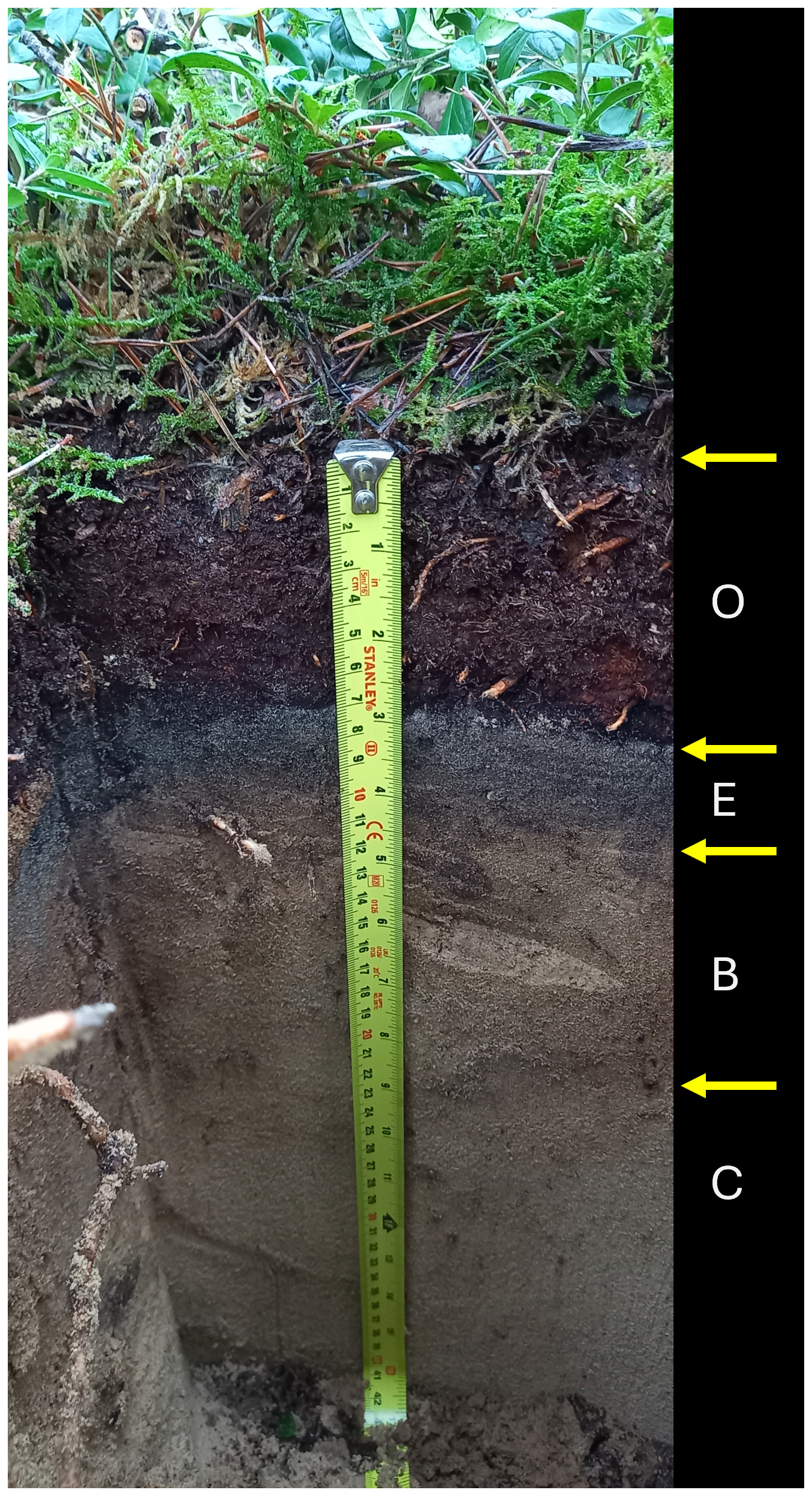
Figure 3Picture of a Podzol soil pit according to the international classification of Mantel et al. (2023), showing understory vegetation consisting of mosses and vaccinium, a 7 cm thick organic (O) layer, 3 cm thick grey leaching layer (E), a 10–12 cm yellow-red illuviation layer (B), and below the yellow-white parent material (C). Note that the boundary between organic and mineral soil is very sharp, which is a sign of absence of mixing by (micro-)organisms. Picture taken at SP-I_12 (see Sect. 2.8.3) on 24 January 2024.
1.2 Ecosystem composition and above ground carbon content
As part of the ICOS labelling procedure (ICOS ETC, 2026), a tree inventory was performed in spring 2023, the results of which provide information about ecosystem composition and provides an estimate of the above ground biomass (Gielen et al., 2017).
1.2.1 Tree inventory
In two Continuous Plots (CP) with a 25 m radius and 20 Spatial sampling Plots (SP) with a 15 m radius (Papale and Nicolini, 2016), all trees with a diameter larger than 5 cm at 1.3 m height were identified. Their GPS locations were measured with a sensitive GNSS receiver (EMLID, Hungary), which, below the canopy, was accurate to within 10 cm. The tree species, diameter and height were identified as well as the health status (Healthy, Minor diseases, Major diseases, Dead, Fallen). All trees were tagged with a unique ID. Tree stumps that fork at or below 1.3 m, were treated as individual trees sharing a common stump. The locations of the CP and SP locations are shown in Fig. 4. The inventory resulted in a database with 1063 trees. The inventory was first done in spring 2023 and according to ICOS instructions will be repeated every 3 years at the CP's and every 10 years at the SP's.
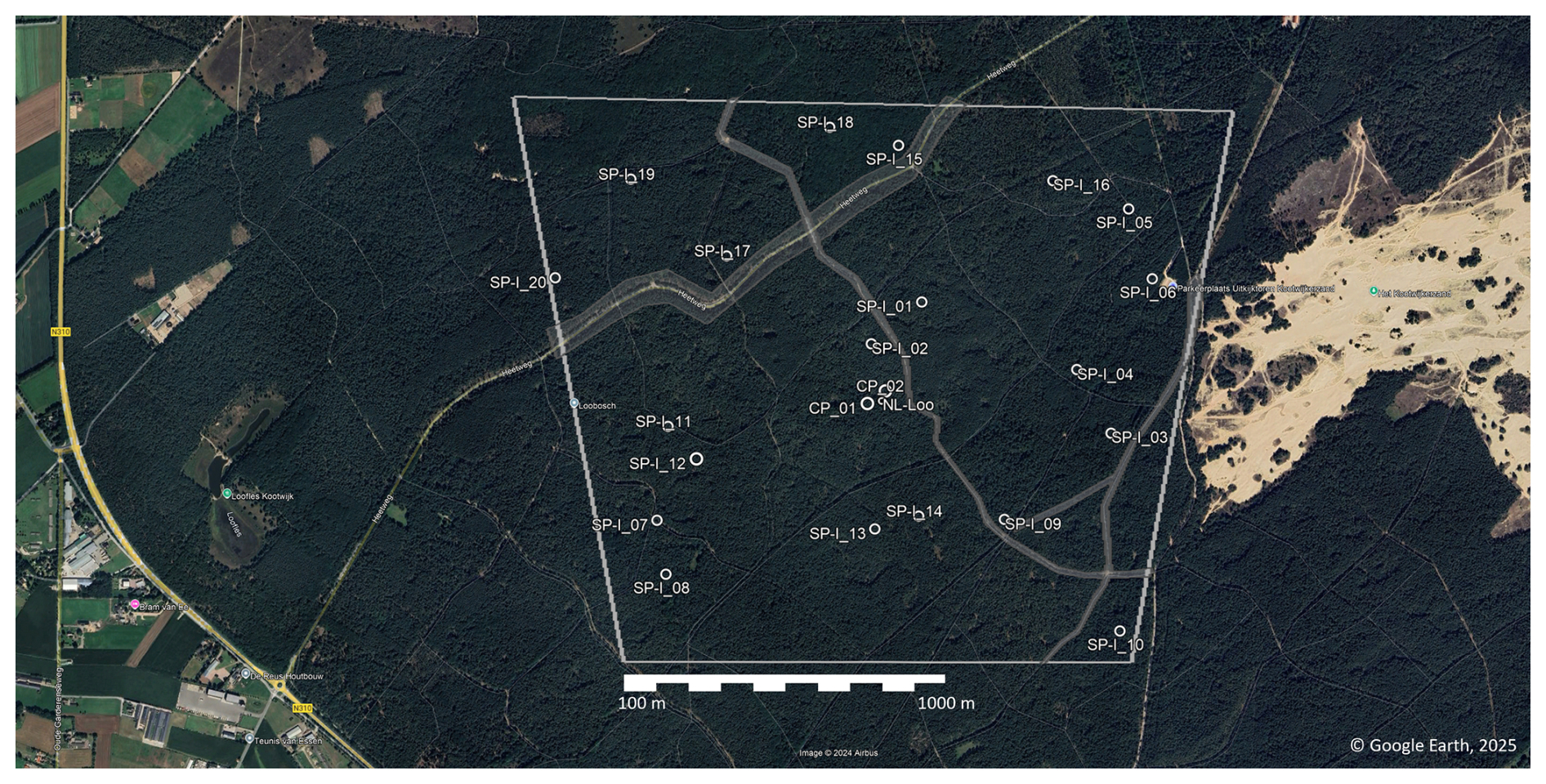
Figure 4Location of the study area, including the target area (grey box) and the Spatial sampling plots (SP-I). The grey shaded surfaces indicate the location of roads and horse tracks excluded from potential selection for SP locations. The location of the tower is indicated by the “o” sign marked “NL-Loo”. The CP's are located in the immediate location of the tower, with CP_01 west of the tower and CP_02 northeast of the tower. The “target area” is the area of which we aim to understand the carbon and water fluxes and other processes (Map data © 2026 Google).
1.2.2 Species composition
Pinus sylvestris L. is by far the most dominant species sampled, with 651 of all 1063 trees. Table 1 lists the total list of species and their health status (Iserbyt et al., 2026). The “health status” has 6 categories:
-
“Healthy”: no visual indication of damage, but healthy leaves are still present;
-
“Minor diseases”: visual indication of the crown being affected by diseases, herbivory, storm damage. The crown is affected by less than 50 %;
-
“Major diseases”: visual indication of the crown being affected by diseases, herbivory, storm damage. The crown is affected by more than 50 %;
-
“Dead” trees: are the ones still standing;
-
“Fallen” are the ones fallen over.
-
“Removed”: this category did not occur in Loobos.
Here “damage” is defined as by branches that have lost leaves or where leaves have changed colour. These definitions are according to the ICOS Instruction for ancillary vegetation measurements in forest (2021).
Table 1List of species observed in the 2023 inventory in the CP's and SP's (Fig. 4) and their health status.
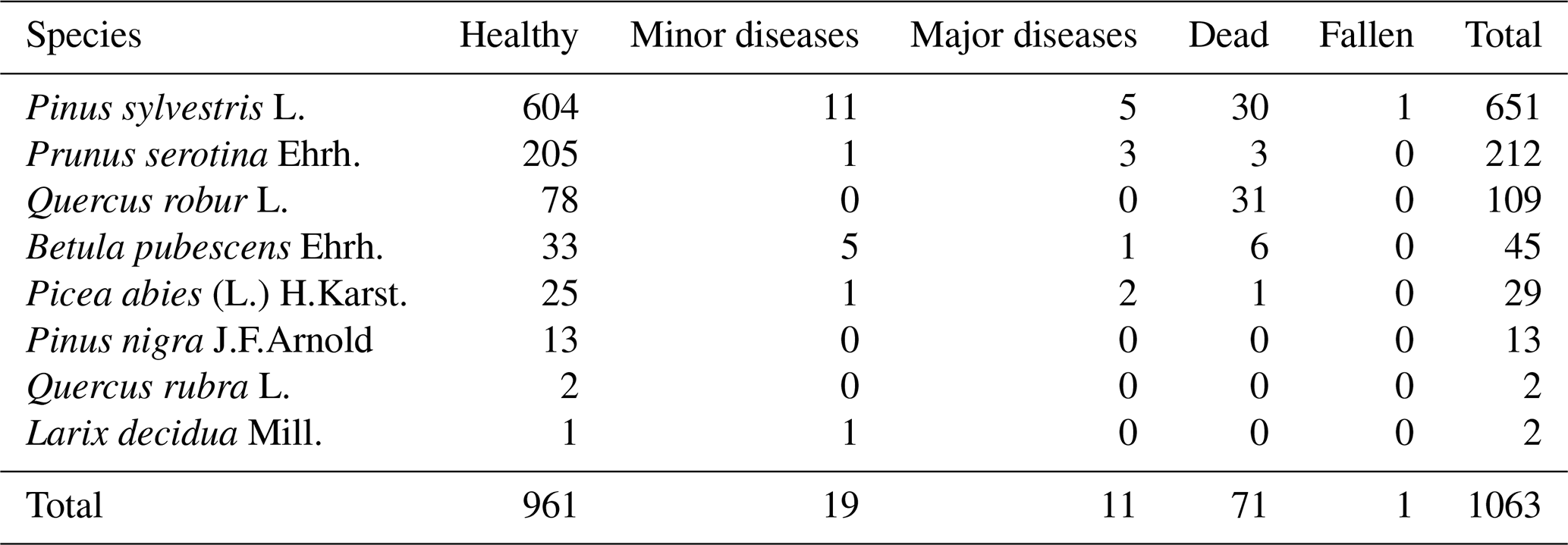
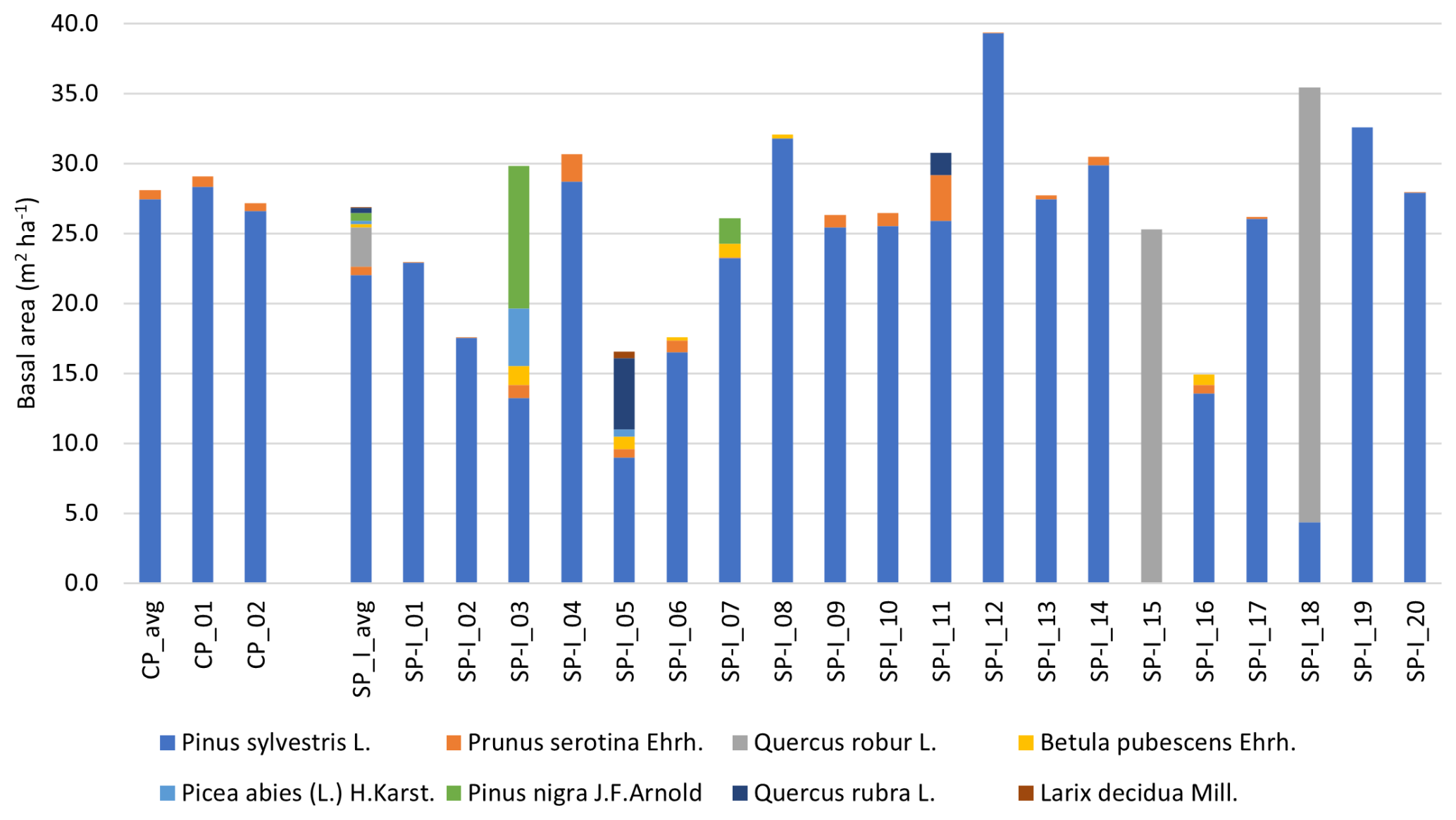
The Prunus Serotina Ehrh. is an exotic invasive species common in the area. It grows below the Pine canopy often in small shrubs (max 3 m tall), sometimes growing in a tree-like shape up to 7 m tall. The species is not managed and was found to be encroaching the area from about 2000 onwards. Recently, in some parts of the footprint of the tower, the majority of the Prunus shrubs have died, perhaps as a result of extreme drought conditions in 2018 and 2023 and a relatively shallow rooting zone. Another theory is that endemic fungi species such as Taphrina farlowii have started growing on the Prunus serotina (Dutch Mycological Association, 2017). However, this Prunus dying did not largely impact their biomass in the CP's and SP's yet. The Quercus robur L. were all observed in SP-I_15 and SP-I_18, where they are almost the only tree species. It is unknown if these oak trees were planted around the same time as the Pine trees. Apart from these two oak plots, the species composition is comparable between the CP's and SP's (Fig. 5). The average tree density is 478 trees ha−1 in the CP's and 568 trees ha−1 in the SP's (505 when excluding SP_I-03), so the area weighted average tree density is 499.1 trees ha−1 in 2023.
The basal area is 27 m2 ha−1 on average over all plots (Figs. 5 and 6). SP-I_05 and SP-I_16 are in a more open part of the forest, which has been potentially subject to thinning. The basal area is dominated by Pine there too. In 2002 an inventory based on 36 randomly selected trees in the same target area resulted in a basal area of 21.4 m2 ha−1, suggesting an increase of 30 % in 21 years.
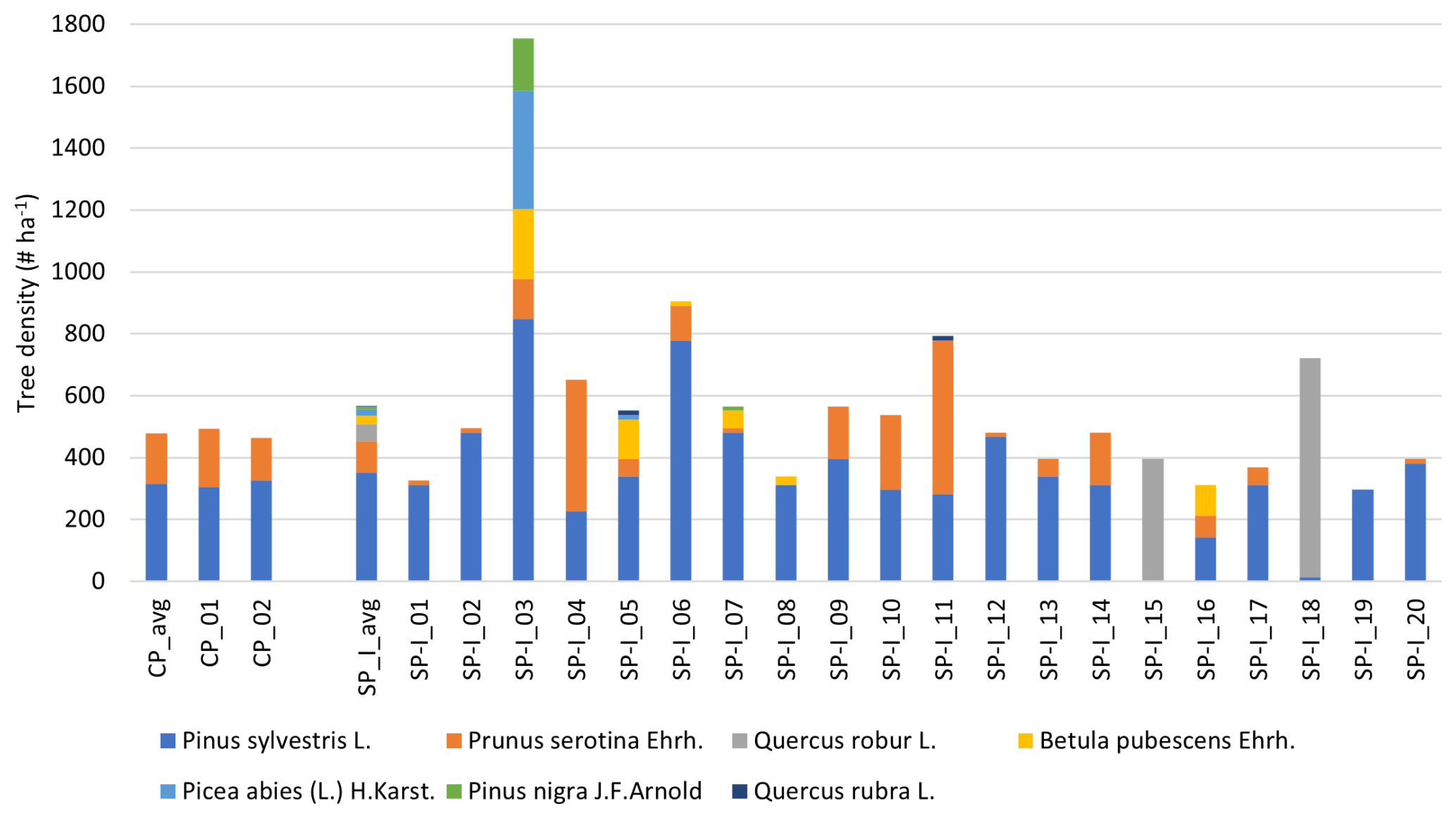
Figure 5Ecosystem species composition in terms of live tree density (# ha−1) in the CP's and SP's, according to the inventory in spring 2023.
1.2.3 Diameter and height distributions
Figure 7 shows the relative diameter at 1.3 m distribution (Iserbyt et al., 2026). It indicates that the trees dominating the total above ground biomass have a diameter centred around 30 cm (Pinus sylvestris L.) and 20 cm (Quercus rubur L.). The Prunus serotina Ehrh. shrubs and Betula pubescens Ehrh. have diameters centred around 10 cm. The average diameter is 21.3 cm for all trees and 25.0 cm for all non-Prunus serotina trees. Earlier tree inventories in the same target area, but with less samples, show a somewhat larger diameter (Table 5 in Zhao et al., 2026) and an average increase of 0.20 cm yr−1.
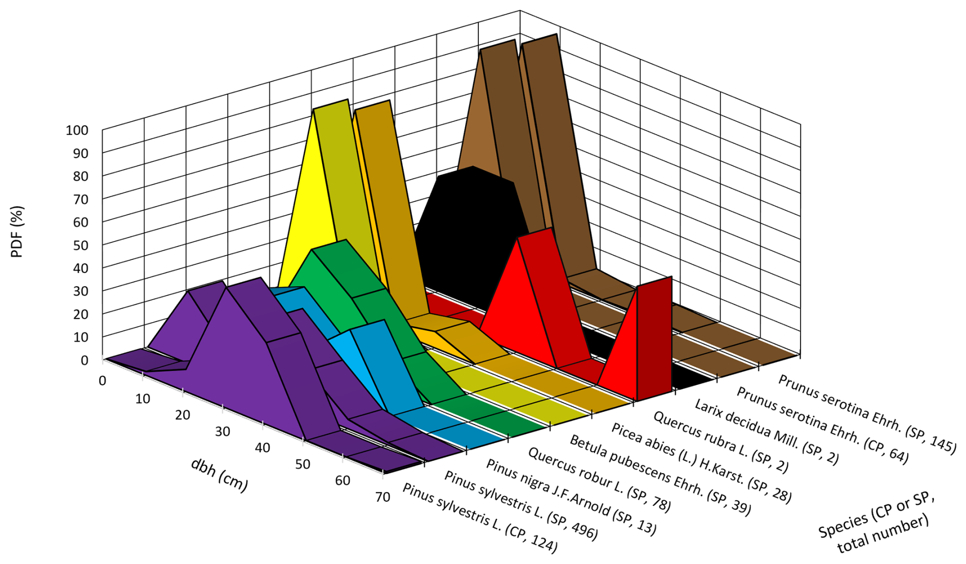
Figure 7Relative distribution of dbh per species in CP's and SP's. The centre of the 10 cm wide diameter classes is shown on the x-axis. The text labels on the y-axes indicate the species and in parentheses the plot type (CP or SP) and the total number of trees in that category. Dbh (cm) denotes diameter at 1.3 m height, and pdf (%) denotes probability density function.
Table 2 shows the average tree height (Iserbyt et al., 2026). It must be noted that the top of the canopy is smoother than the surface topography, because the tree height is inversely related to the dune height, i.e. trees on dunes are shorter than trees in valleys between the dunes, based on airborne lidar data collected in 2022. Since the tower's base is in a valley and many of the trees around it are on dune slopes and tops, the average canopy height appears to be a height of 20 to 22 m relative to the tower.
Table 2Average tree height (m) ± 1 standard deviation in the CP's and SP's in 2023.
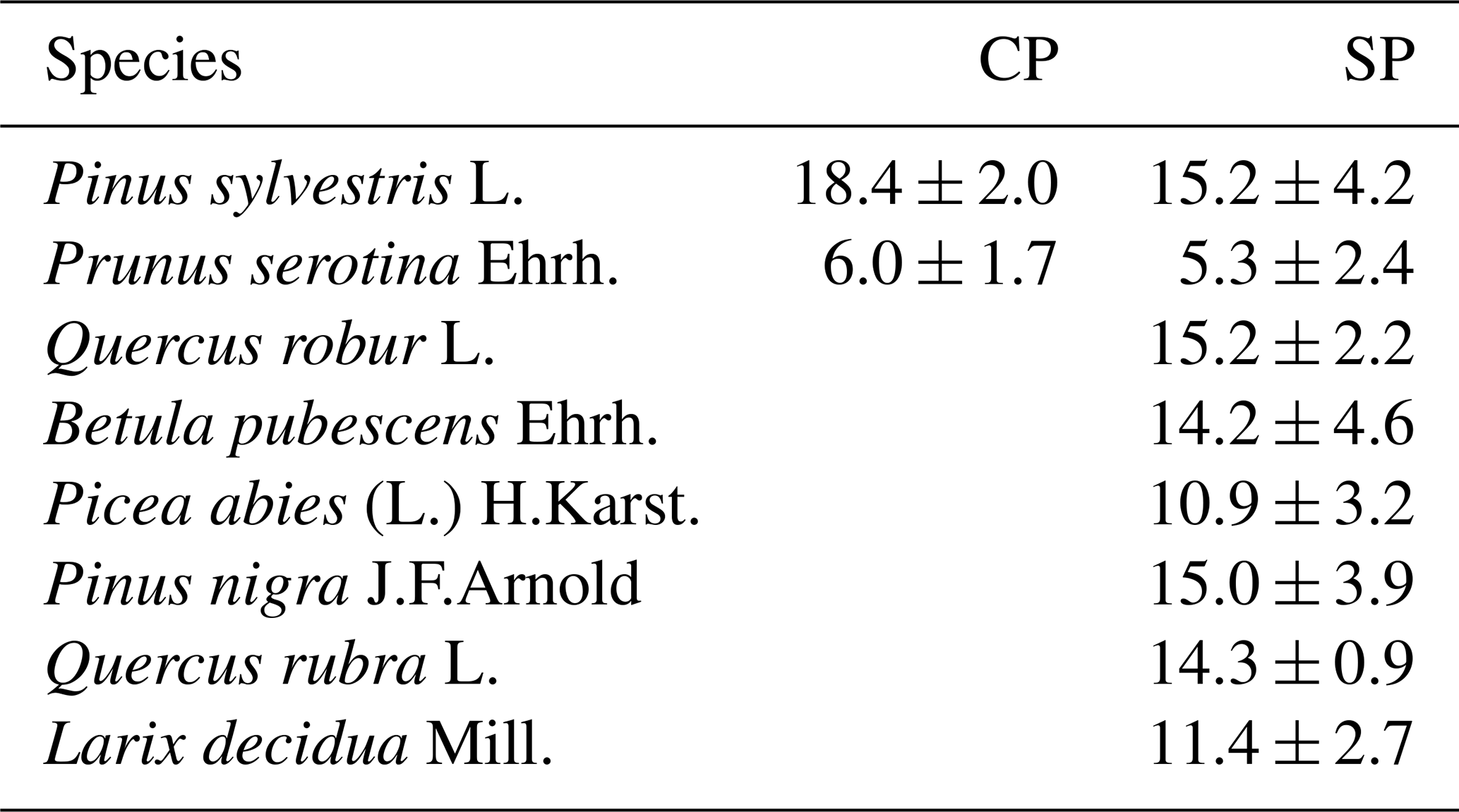
This tree height matches well with tree height measured another plot in the target area in earlier years (Table 4 in Zhao et al., 2026). These data suggest a growth rate of 16 cm yr−1. This would extrapolate to an average height of 19.6 m in 2023, which is somewhat taller than the observed height in 2023. However, the diameters reported for these trees are larger too. We hypothesize that the difference is caused by the difference in sample size and geographic distribution of the plots. However, this should be studied in more detail in the near future.
1.2.4 Allometric relations and biomass
To estimate the biomass from the tree diameter, height and species, we used allometric relations. We adopted the relations used in the 7th Dutch Forest Inventory (Schelhaas et al., 2022). The inventory uses Eq. (1) to estimate the mass of stem wood and bark:
Where mstem+bark refers to the mass of stem wood and bark in kg, ρw refers to the wood density, dtree and htree to the tree diameter at 1.3 m and the tree height. α, β and γ are specie-specific parameters, the values of which can be found in Table 3. The mass of branches (living and dead), leaves and roots is estimated with Eq. (2):
where mX is the mass in kg dry biomass and X refers to the categories “branches”, “leaves” and “roots”. κ, λ and μ are species and category dependent parameters (Table 3). Note that the ICOS biomass inventory (Iserbyt et al., 2026) focuses only on aboveground biomass, so we will omit the biomass of roots (although giving the parameters for completeness).
Table 3Parameters to Eqs. (1) and (2) for estimating tree biomass.
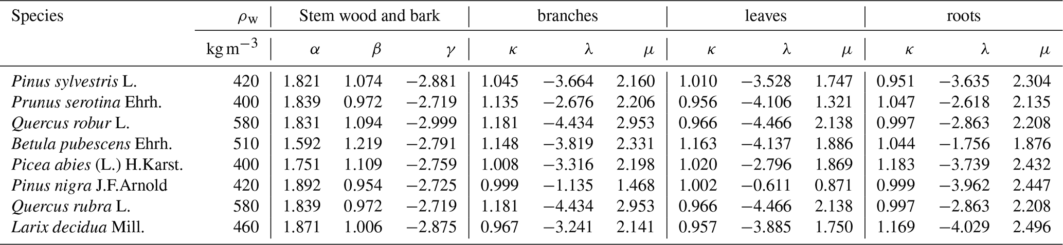
Table 4Mean ± standard deviation of dry above ground biomass in t ha−1 of live trees estimated using the 2023 tree inventory and allometric relations given above. The means and standard deviations are calculated over 2 CP's and 20 SP's. The dead above ground biomass is not part of the “Total” (van der Molen et al., 2026a).
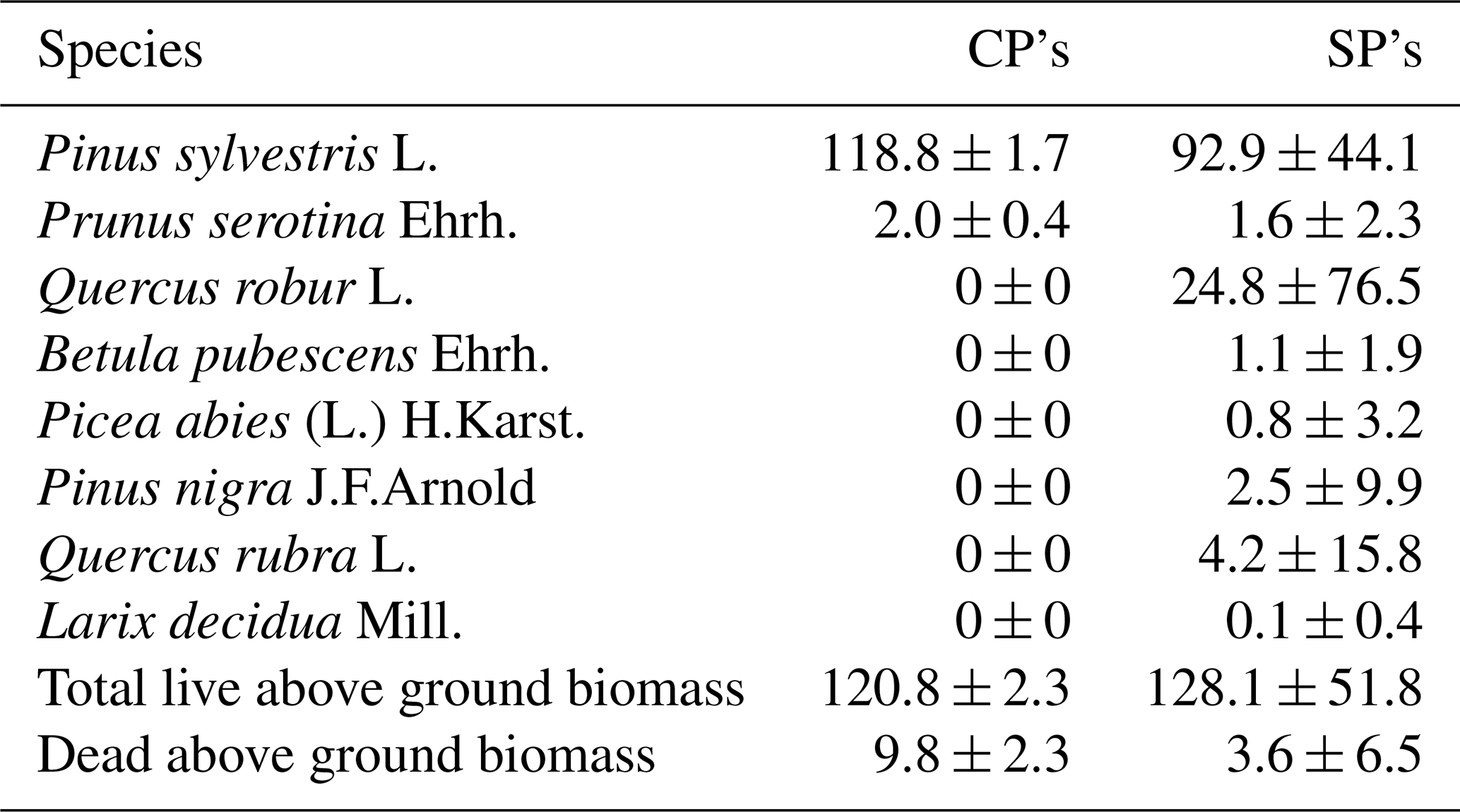
In a separate plot used in earlier inventories, the above ground biomass was estimated at 121 t ha−1 in 2000, increasing to 151 and 173 t ha−1 in 2012 and 2025 (Table 6 in Zhao et al., 2026). Their data suggests a larger biomass, based on fewer trees (N = 56–103), than the 2023 inventory (N = 1000 trees). Nevertheless, their estimated biomass is comparable, albeit at the larger end of the range of the estimates for the SP's.
The accuracy of those estimates depends on the number of trees measured and the spatial variability, the quality of the measurements, the quality of the allometric relations and the associated parameters. At present, a detailed uncertainty analysis is not available. It is remarkable that the 1996–2025 biomass estimates show a consistent increase, whereas the 2023 estimate (based on more trees in a wider footprint) results in a 35 t ha−1 lower aboveground biomass. The standard deviation of above ground biomass between the SPs is 51.8 t ha−1 and the contribution of standing dead trees is 9.8 t ha−1 in the CPs (3.6 in the SPs). This suggests that spatial variability and dying trees could be responsible for the difference in the 1996–2025 and 2023 ICOS inventories. The accuracy of the allometric relations applied will affect the absolute value of the above ground biomass estimates more than changes in time.
As such, Loobos has a somewhat lower dry above ground biomass than the average in Dutch forests of 177.3 t dry above ground biomass ha−1 (Schelhaas et al., 2022, Table 13.1). However, it is rather similar to the biomass estimated at the ICOS station in Brasschaat, Belgium (BE-Bra), which has a comparable pine ecosystem and a biomass of 117 t ha−1 in the CP's in 2023 and 102 t ha−1 in the SP's in 2020, based on the ICOS conform tree inventory at that station.
In this section we describe the tower and its instrumentation in separate sections for (1) infrastructure, (2) radiation measurements, (3) soil measurements, (4) meteorological measurements, (5) ICOS eddy covariance measurements, (6) vertical profile measurements, (7) additional concentration and flux measurements of VOC's and ozone, (8) intermittent ecosystem measurements and (9) occasional campaigns. We summarise the instruments and the variables per section in a table. The table contains the instrument type, manufacturer and model, the serial number (SN), the instrument height, eastward and northward distance with respect to the centre of the tower's base and the names of the variables measured.
According to the ICOS instructions, the variable names have subscripts H, V and R, where H refers to the horizontal index number, V to the vertical index number and R to the replication index number. For example, in a single vertical soil profile, each instrument has the same H index and consecutive V indices. If a sensor is added in proximity to another one measuring the same variable, the R index is raised. A second soil profile has a higher H index and can have the same V-indices.
2.1 Infrastructure: Tower, power and internet connection
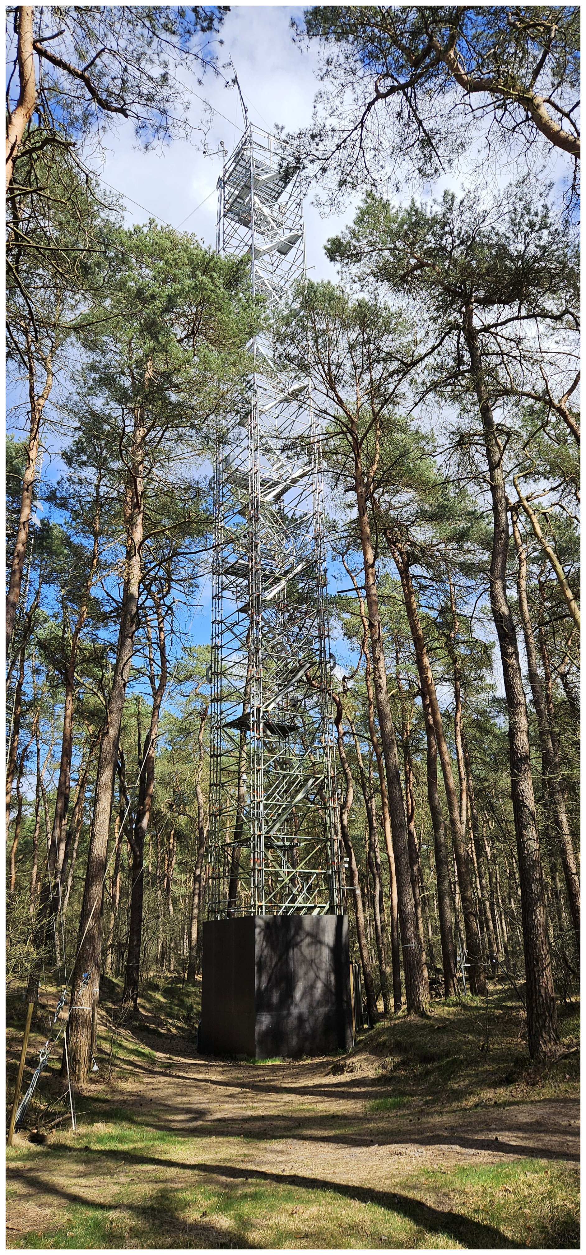
The tower is built of scaffolding material (Layher) with a surface spanning 2.57 m × 2.57 m. Stairways lead one up the tower. The highest platform is at 36 m (Fig. 8). In that picture, the left corner points towards the North and the right one to the South. The station coordinates in the WGS 84 system are: Latitude 52.16644722° N and Longitude 743555° E. The UTC offset is equal to +01 h and the elevation is 24 m a.s.l. The site is marked by the following climate characteristics: mean annual (above canopy) temperature 10.2 °C, mean annual precipitation 900 mm and mean annual global incoming radiation 114 W m−2, positioning it in the temperate oceanic climate (Cfb) Köppen-Geiger climate classification (Geiger, 1954). Next to the tower (Fig. 8) a shipping container is placed, where electricity is available (3×25 A, 19 kW). A local area network is present, with a 4G connection to the internet.
2.2 Radiation measurements and PhenoCam
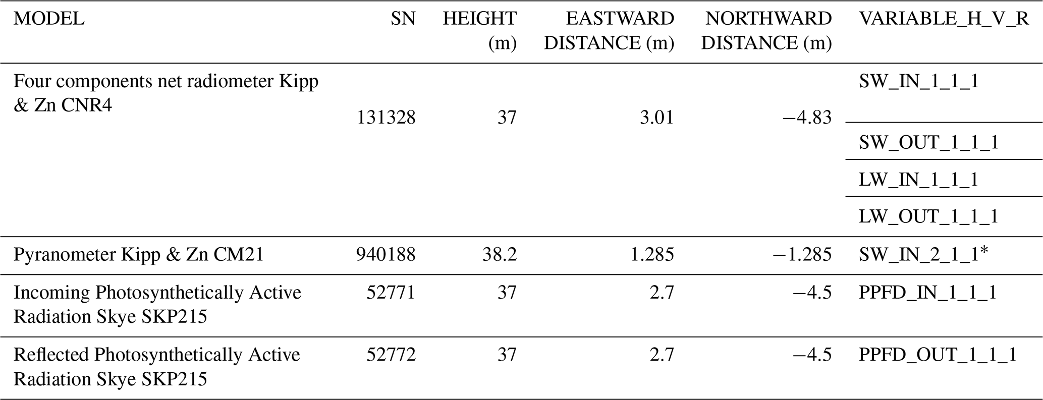
Four component (shortwave and longwave, incoming and reflected/outgoing) radiation measurements are made with a CNR4 radiometer (Kipp & Zonen, Table 5). The instrument is mounted on a 3.52 m long pole pointing towards the southwest from the southern point of the tower at a height of 37 m, 15 m above the canopy top. The instrument is equipped with a level (roll and pitch), which are logged with the data and used to level the instrument after cleaning. A backup global radiometer (CM21, Kipp & Zonen) was installed at the top of the tower at 38.2 m.
Incoming and reflected photosynthetically active radiation are measured with two SKP215 PAR Quantum sensors, mounted on the same pole as the CNR-4 (Table 5). The PAR sensors are sensitive to radiation of wavelengths between 400 and 700 nm.
The CNR4 and PAR instruments measuring incoming radiation do not suffer from shadows cast by the tower or other structures. The backup global radiometer is exposed to a daily shadow from the lightning deflector. The instruments measuring reflected/outgoing radiation have the tower in about 10 % of its field of view. All radiometer data are sampled and stored at an interval of 2 s. These data are available via the ICOS Carbon Portal (van der Molen et al., 2026b, c, f, g).
Table 5Specification of radiometers. * SW_IN_2_1_1 is part of the backup meteorology system (Sect. 2.4). The heights, east and westward distances are defined relative to the reference point, which is the centre of the tower's base.
A StarDot Netcam SC5 IR was installed at 35 m height in the tower facing the North. Images are collected hourly from 10:30 to 17:30 CET. Until 28 May 2026, images we automatically uploaded to “PhenoCam, an Ecosystem Phenology Camera Network” operated by the Northern Arizona University (Richardson et al., 2018) and automatically analysed for green chromatic coordinate (GCC) and normalised difference vegetation index (NDVI). All images and results can be viewed via PhenoCam (2026) (Richardson et al., 2018; Seyednasrollah et al., 2019). The GCC and NDVI time series show similarity with the LAI measurements (Zhao et al., 2026), i.e. a peak in August and low values between November and April. After 28 May 2026, ICOS took over the function of the phenocam network in Europe. Data are now uploaded to the ICOS Carbon Portal (2026) and the resulting analyses via Iserbyt et al. (2026). Content-wise, nothing has changed in the data processing and analysis.
2.3 Continuous soil measurements
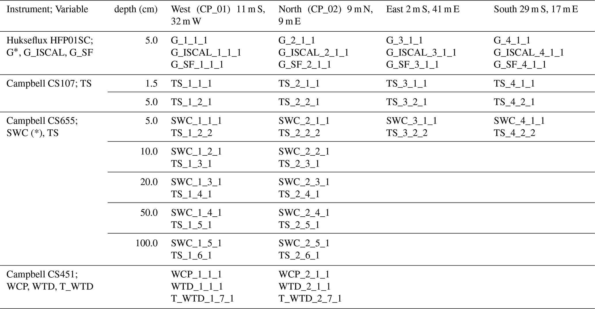
Continuous soil measurements are taken at 4 plots around the tower (Fig. S1). At each plot, the soil heat flux (G) is measured at 5.0 cm depth along with soil temperature (TS) at 1.5 and 5.0 cm deep (Campbell CS107), as well as soil water content (SWC). Only at the West and North locations, water table depth (WTD) and a deeper profile of SWC and TS are measured, at depths of 5, 10, 20, 50 and 100 cm. Table 6 provides a complete overview over which variables are measured at which plot with what instrument model. The West plot is on the SE facing flank of a dune, the North plot is on top of a 2 m high dune underneath the first tower, within centimetres from the soil sensors associated with the first tower, to continue the first tower's time series. The East and South plots are in a valley between the dunes.
The soil heat flux plates (Hukseflux HFP01SC) are self-calibrating. One of the plates self-calibrates every third hour in a N-E-S-W rotation starting at midnight. During the self-calibration, the flag variable G_ISCAL is set to 1. The latest sensitivity factor is stored in the variable G_SF.
The WTD sensor measures the pressure of the soil water column above it and hence the reading depends on the installation depth. The West WTD sensor's head is 8.88 m below the tower's base and the North sensor's head 9.59 m. Hence it follows that WTD_1_1_1 (m) is related to WCP_1_1_1 (Pa) as:
and WTD_2_1_1 (m) is related to WCP_2_1_1 (Pa) as:
with ρw = 998.2 kg m−3 at 20 °C and g = 9.81 m s−2. ETC processes these data following these equations, and the meta information needed, such as the installation depths, are reported via a standard protocol (BADM). All soil variables are logged by a single Campbell CR1000X datalogger at a sample interval of 1 min. These data are available via van der Molen et al. (2026b, c, f, g).
Table 6Continuous soil measurements. G: Soil heat flux (W m−2), G_ISCAL: Flag for measurements during self-calibration (1 = yes, 0 = no), G_SF: Sensitivity Factor (V/(W m−2)), TS: Soil Temperature (°C), SWC: Soil Water Content (m3 m−3), WCP: Water Column Pressure (Pa), WTD: Water Table Depth (m), T_WTD: Soil Temperature from WTD sensor. The header row indicates the location of the plots relative to the centre of the tower. The variables marked with * are logged as raw voltages too.
2.4 Precipitation, air pressure, temperature, humidity and backup system
Precipitation (P_1_1_1) is measured with a MPS TRwS 4E15 weighing rain gauge. The rain gauge is installed in a separate tower 57.7 m North and 25.7 m East of the tower's base at a height of 15.3 m. As such it is located in a small opening in the forest where the surrounding trees function as a wind shield. The horizontal distance to the tree tops is 2 to 4 times the height difference (i.e. the angles are between 14 and 26.5°).
Air pressure is measured with a Bosch BMP390 at a height of 35 m in the tower. The height difference between the sensor and the tower base is not corrected for, nor is the pressure converted to sea level pressure.
Air temperature (TA_1_1_1) and relative humidity (RH_1_1_1) are measured at the top of the tower at 38.2 m with a mechanically ventilated and sun shielded Vaisala HMP155 (Sect. 2.6 describes their vertical profiles). The sample collection and storage interval are both 20 s.
A backup meteorological system is installed, intended to measure a few variables, key for applying the ICOS gapfilling procedure (ONEFLUX, Pastorello et al., 2020), in case a power or system failure occurs. The backup system operates entirely independently from the other systems and is powered by a battery. It consists of a Campbell CR1000X datalogger, powered by a battery, which is charged from a separate group in the electrical distribution box. The datalogger logs the signals of the Kipp & Zn CM21 Pyranometer (SW_IN_2_1_1, 38.2 m, Sect. 2.2), a second Vaisala HMP155 sensor (TA_3_1_1 and RH_2_1_1, 38.2 m, Sect. 2.6) and a Young 52203 rain gauge (P_2_1_1, 37.7 m). Each of these instruments is installed at the top of the tower. The backup rain gauge is not shielded, which causes the observed precipitation to be underestimated by about 10 % relative to the precipitation observed by the weighing rain gauge, shielded by the tree tops (P_1_1_1). The sample collection and storage interval are 20 s. These data are available via van der Molen et al. (2026b, c, f, g).
2.5 ICOS compliant eddy covariance measurements
Turbulent flux measurements are carried out with the eddy covariance technique using a Gill HS-50 ultrasonic anemometer and a Li-COR LI7200RS enclosed CO2 and H2O gas analyser mounted on top of the tower at 38.2 m, ∼ 16 m above the forest canopy. The horizontal head of the anemometer is directed towards the prevailing wind direction (SW), 1.75 m outside the tower structure. The gas analyser is mounted downwind from the anemometer and draws in air from just outside the anemometer's sample volume via a 0.71 m long 6 W heated tube with an inner diameter of 5.33 mm and a flow rate of 10 L min−1. The anemometer measured three components of wind velocity and sonic temperature at 50 Hz. The gas analyser measures CO2 and H2O concentration at 20 Hz. Signals from both instruments are collected by a Li-COR Smartflux2 system, which co-locates both data streams with GPS time to an output with frequency 20 Hz (Fratini et al., 2018). This setup is compliant with the ICOS instructions (Sabbatini and Papale, 2017). More specifications are provided in Table 7.
The 20 Hz data are collected in zipped 30 min CSV files. These files are sent to the ICOS Carbon Portal for further processing of the raw data into fluxes, quality assurance and gap filling. The raw as well as the processed data can be retrieved from the ICOS Carbon Portal (2026) and in van der Molen et al. (2026d, h).
Figure 9 shows the climatological footprint of the eddy covariance fluxes around the tower, where the 50 %, 70 %, 80 % and 90 % cumulative footprint isopleths (Kljun et al., 2015) are shown with respect to the target area in unstable () and stable () conditions. The typical radius of the 80 % isopleth is 270 m in unstable conditions and 500 m in stable conditions. Even the 90 % footprint is almost entirely within the target area. The flux data are available via van der Molen et al. (2026d, e, f, i).
Table 7Technical specifications of the eddy covariance system.
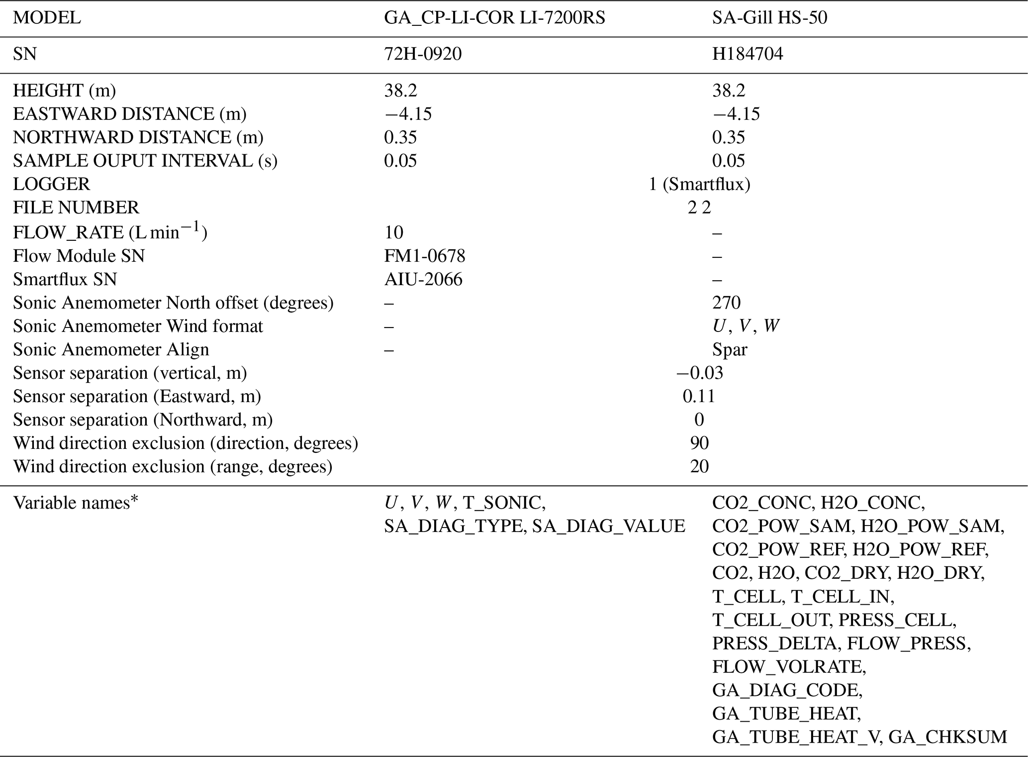
* These variable names do not follow the _H_V_R notation.
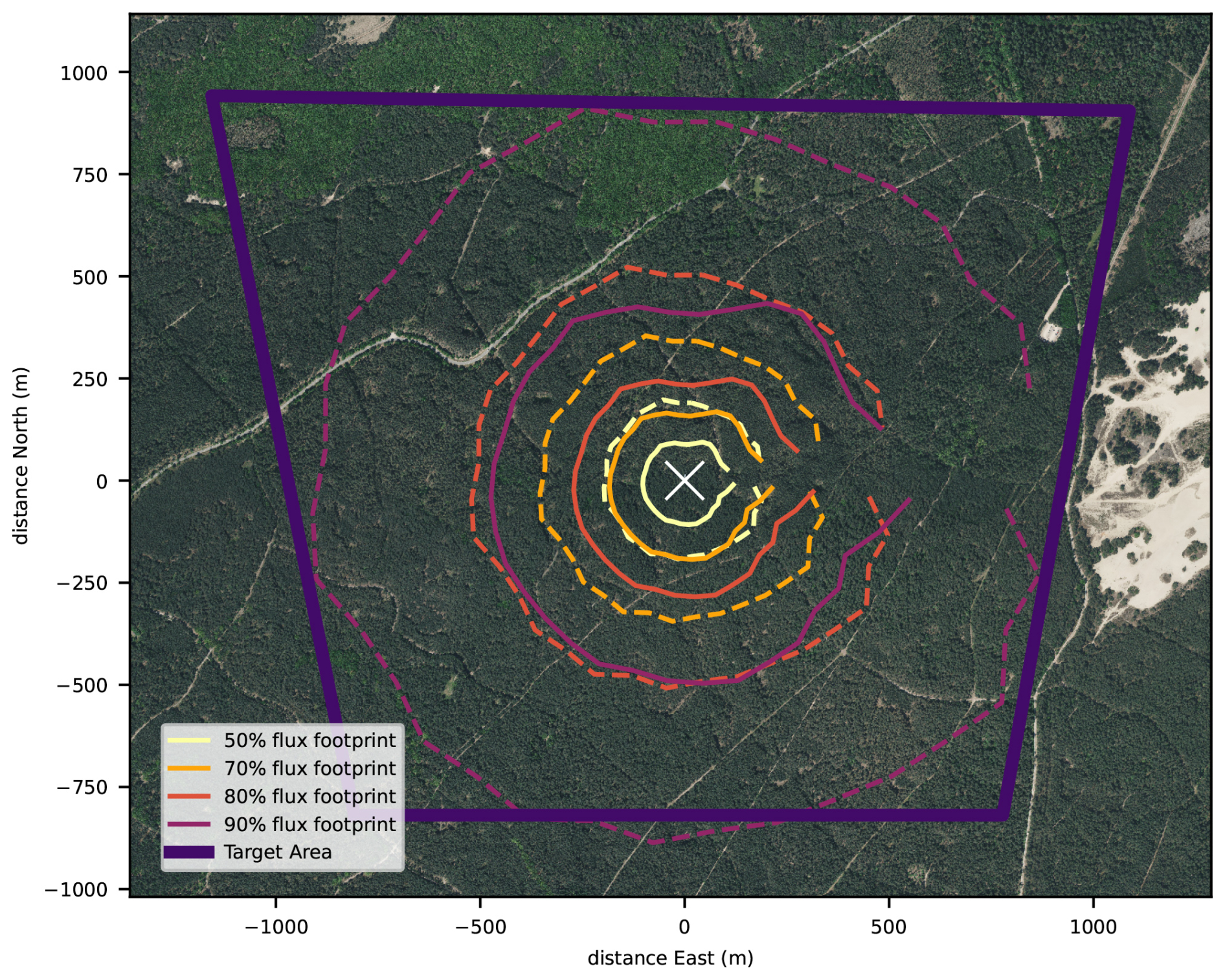
Figure 9Footprint climatology of the turbulent fluxes measured at the EC tower in relation to the extent of the target area. The 50 %, 70 %, 80 % and 90 % cumulative contribution isopleths are shown. The solid lines represent the footprint area in unstable conditions () and the dashed lines in stable conditions (). The white crossmark in the center indicates the location of the tower. The isopleths are interrupted towards the east, because this area is excluded from flux calculations, as the tower may distort the wind flow and the turbulence field characteristiscs from those areas. (Background aerial photograph 8 cm RGB, pdok.nl, 2026).
2.6 Vertical profiles of CO2 and H2O concentrations, temperature, wind speed and direction and leaf wetness
The eddy covariance system is installed at a height of 38.2 m, while the tree canopy is densest roughly between 16 and 22 m. Hence in stable atmospheric conditions, turbulence may not be strong enough to mix air from the ground and canopy space to the height of the eddy covariance system. Hence emissions (or deposition) of gases, moisture and heat, may lead to the accumulation (or depletion) of concentrations and heat in the below-canopy space and remain (partially) undetected as turbulent fluxes by the eddy covariance system. After transitioning to an unstable atmosphere, the gases, moisture and heat will be mixed to the level of the eddy covariance system again and cause a delayed response. Assuming no net horizontal advection, the sum of accumulation in stable conditions and release in unstable conditions over a day is supposedly zero over 24 h (strictly speaking between well mixed moments, e.g., afternoons of consecutive days).
To quantify the below-canopy storage of CO2, water vapour and heat, these variables are measured along a vertical profile along the tower. CO2 and H2O mixing ratios are measured at 11 levels and temperature at 5 levels (Table 8). In addition, we also measure wind speed and direction at 5 levels in order to characterise below-canopy wind flow. The wind speed and direction profile measurements are not mandatory for ICOS, but still submitted to the carbon portal. The number of 11 levels is chosen such that interpolation errors do not account for more than 5 % of the relative flux. The distribution of levels follows a logarithmic profile, which is slightly adapted to the levels of the platform in the tower to access the instruments. From the change in concentrations and temperature in time and the thickness of the representative air space, the accumulated CO2, water vapour and heat are calculated as:
where F represents the so-called storage flux, dt the integration time (30 min in this study), z the height along the tower, hEC the height of the eddy covariance system (38.2 m), and X the variable (i.e., CO2, H2O or temperature). The storage fluxes are calculated by ICOS ETC after submission of daily data. Analysis of measurements along a profile in the first tower (Zhao et al., 2026) shows that storage fluxes of CO2 may be in the order of −5 and +3 µmol m−2 s−1, hence making up a relatively large part of the total fluxes. For water vapour and heat, the contribution of the storage fluxes is considerably smaller. Hence the resolution of the CO2 (and H2O) profile is finer than for temperature.
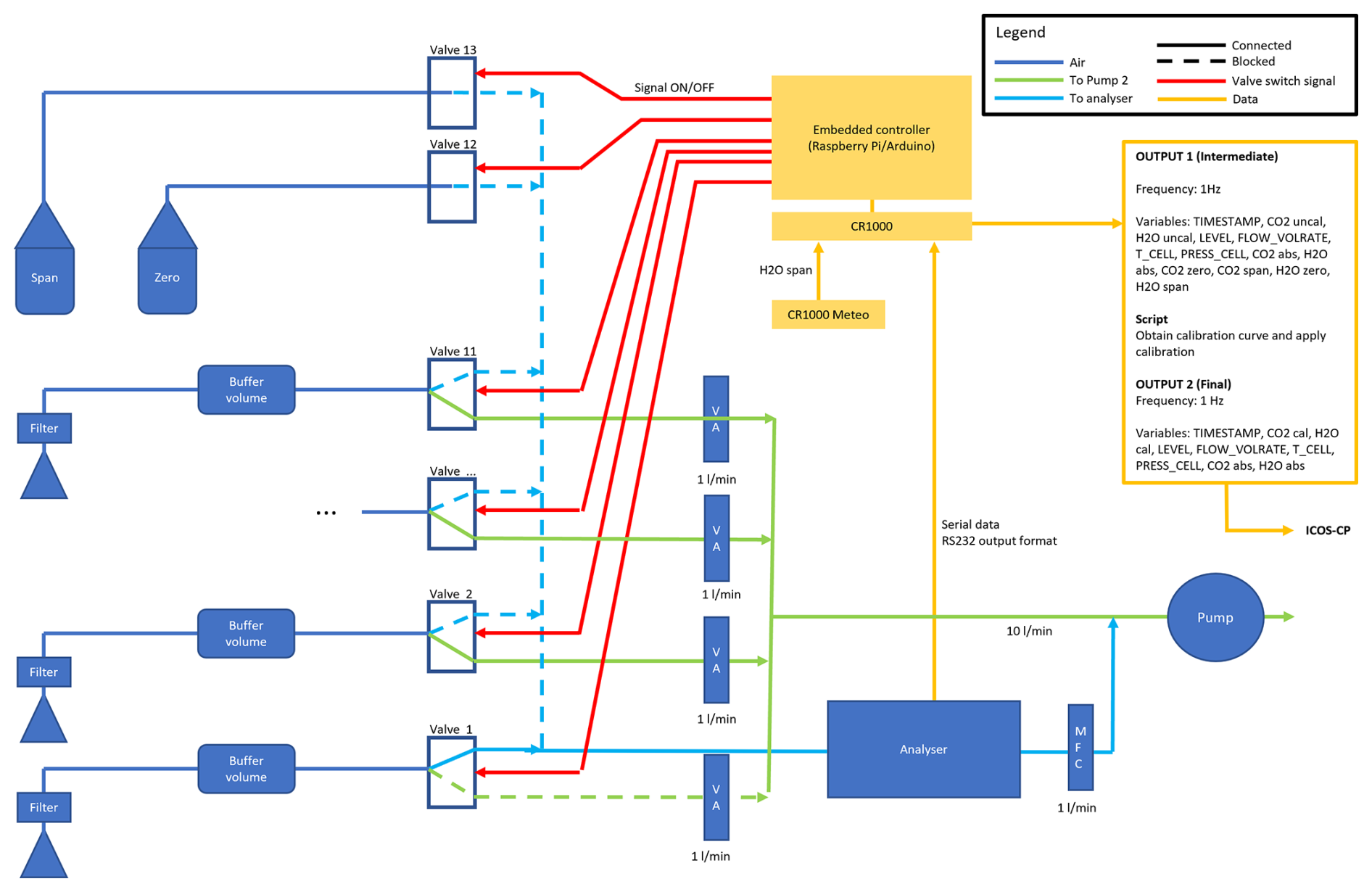
A single Li-COR LI-850 gas analyser is employed to sequentially measure the concentrations at each of the 11 levels (Fig. 10). The inlets are protected with precipitation shields. At the inlets, an air suction filter (ZFC 050-04B, SMC, Japan) is installed to filter out particulate matter (5 µm, 95 % filtration efficiency) and to reduce pressure to about 80 kPa to prevent condensation in the tubing. The air is then drawn to a 3.5 L buffer volume (DURAN™ GLS 80™) to dampen short-term variations in concentrations. Behind the buffer volumes, the tubes are connected to 3-way pneumatic solenoid valves (EVT317V-6DZ-02). One end of each outlet is connected to a mass flow regulator (EL-FLOW Base F-201CB, Bronkhorst, the Netherlands), which maintains a constant flow rate of 1 L min−1 in each line. The other end of each outlet is connected to the gas analyser, behind which is the same type of mass flow regulator, maintaining 1 L min−1 through the gas analyser as well. All tubes are Teflon (PTFE) with an inner diameter of 4 mm. The use of Teflon was preferred over PUR (Polyurethane) tubes (SMC TU0604B-20), which appeared to incur condensation more than Teflon tubes. All fittings are one-touch fittings (SMC Metric Size KQ2). A 200 L min−1 vacuum pump (Pfeiffer Vacuum HiScroll 12 ATEX) draws the air through each of the lines.
Table 8Vertical profile measurements of CO2 and H2O concentrations, temperature (T), wind speed (WS) and wind direction (WD), relative humidity (RH) and their heights. The third row indicates the instrument model, the fourth row the sample collection frequency and the subsequent rows indicate the variable names. In the case of CO2 and H2O, the variable name is the same for all levels, where a separate variable (LEVEL) indicates the level number. * TA_3_1_1 and RH_2_1_1 are part of the backup meteorology system (Sect. 2.4).
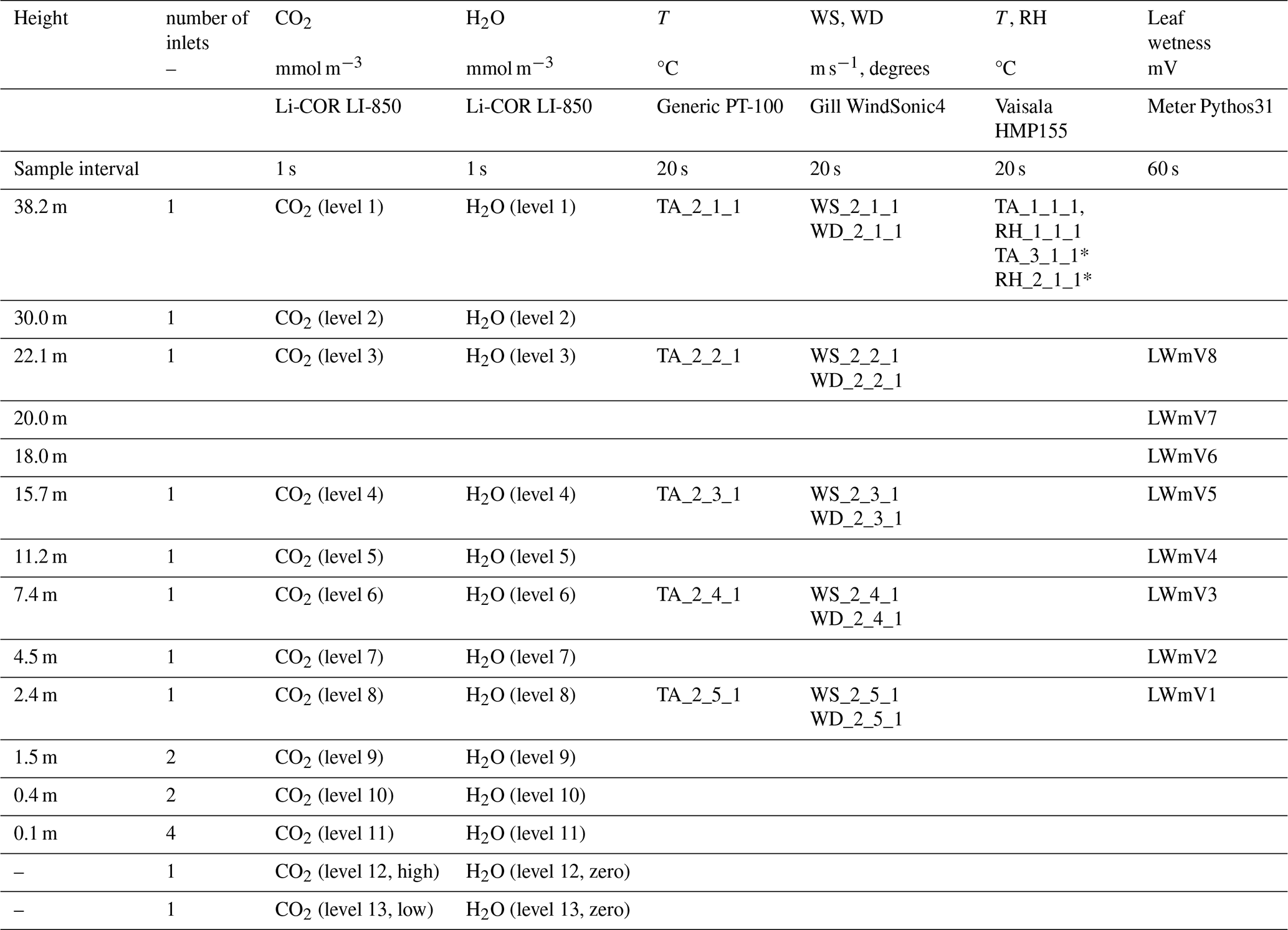
The levels 12 and 13 are connected to gas cylinders with known gas concentrations (464.64 ppm and 367.93 ppm CO2, zero H2O). The two lowermost are ramified with two inlets at 1.5 and 0.4 m and 4 inlets at 0.1 m. The levels below 5 m are installed in a separate mast next to the main tower, as the tower is fenced off with solid multiplex boards (Fig. 8). The tubing is led underground to the buffer volumes. The underground parts are heated about 1 °C above the soil temperature to prevent condensation in the tubes.
A Campbell Scientific CR1000X datalogger logs the gas analyser's digital 1 Hz output. Besides CO2 and H2O concentrations, the volume flow rate (FLOW_VOLRATE), cell temperature and pressure (T_CELL, PRESS_CELL) are sampled. The datalogger also controls the switches via a Raspberry Pi embedded controller. The switches are set every 30 s to sample each of the lines 1 to 11 sequentially. The two calibration gasses (levels 12 and 13) are sampled at midnight (00:00 CET) and noon (12:00 CET) each day for 30 s each. As a result, all levels are sampled with a return time of 5.5 min (6.5 min including calibration levels). A linear least squares regression is used to calibrate the CO2 concentration measurements for the next 12 h. The calibration coefficients are stored. The slopes are typically between 0.95 and 1.05 over a longer period (2 years) and vary with an amplitude less than 0.02 over a month. The instrument's water vapour response is calibrated a few times per year with a Li-COR LI-610 dew point generator. The temperature profile is measured using mechanically ventilated generic PT-100 Class 1/3 DIN thermometers at the 5 levels (Table 8). Gill Windsonic4 at the same 5 levels measure wind speed and wind direction. The profile system is complemented with air temperature and relative humidity measurements with two Vaisala HMP155 sensors, one “regular” (TA_1_1_1 and RH_1_1_1) and one backup (TA_3_1_1 and RH_2_1_1, Sect. 2.4) at the top of the tower. The data are available via the ICOS Carbon Portal (van der Molen et al., 2026a, b, c, d, f, g, h).
A profile of 8 leaf wetness sensors (Meter Environment Pythos31) was installed along the tower in August 2023 (Table 8), from the canopy top downward. The sensors measure the electrical conductance on an artificial leaf surface, which increases with the wetness of the leaves. The sample interval is 1 min. Being non-ICOS standard, these data are only accessible at MAQ-Observations (2026) and especially relevant for analysis of the role of canopy wetness in the exchange of reactive compounds such as nitrogen compounds, ozone and BVOCs.
2.7 Additional eddy covariance measurements of VOC and ozone
Volatile Organic Compound (VOC) and Ozone (O3) concentrations and fluxes are measured at the station since the year 2022 and 2025, respectively. These species interact with the ecosystem's canopy conductance, carbon uptake and transpiration. Regional emissions of reactive oxidized nitrogen, NOx, reactive reduced nitrogen, NHy, and VOCs affect the ozone and reactive nitrogen species chemistry, concentrations and deposition, which influence nutrient availability for plant growth and acidity. We first describe the methods to measure concentrations and then briefly outline the methods of flux calculations. Note that these observations are not standard ICOS measurements.
2.7.1 Concentration measurements
VOC concentrations are measured with a Proton-transfer-reaction mass-spectrometer (PTR-MS). The instrument was installed in November 2022. Ambient air is sampled through a 56 m long PFA tubing (inner diameter = 6 mm) from close by the sonic anemometer at 38.2 m above the ground (Sect. 2.5) to the instrument which is placed in the shipping container (Sect. 2.1). Between the tower and the shipping container the line is led trough a PVC tubing buried 20–30 cm below the ground. Since 14 November 2024, the underground part is heated by a self-regulating tube heating (QUINTEX GmbH, ILLW172CT/QX) to avoid condensation especially during summer. The flow rate is regulated at ∼10 L min−1 (at 0 °C) by a needle valve and the tubing is protected by a filter (PTFE coated quartz fibre filter, 90 mm diameter, in a PFA filter holder ) which is positioned ∼38 m above the ground approximately 2 m from the sonic anemometer. The filter is replaced once every 2–6 weeks to prevent slight flow reductions due gradual buildup of aerosol on the filter. Mixing ratios of VOC's of more than 500 individual masses with a mass-to-charge ratio <1000 Th are measured and recorded at a 2 Hz rate. Each hour, the air is diverted through a heated Pt-filter that burns all VOCs to CO2 and H2O during 10 min, hence reducing the concentrations to zero. This procedure serves as an effective zeroing method. In December 2024 a fast response dry chemiluminescence ozone analyser (Fast Ozone Sensor, Sextant Technologies) was installed. The instrument was installed in a heat insulated box in the tower at 35 m with a 5.5 m long 4 mm diameter Teflon tube to an inlet close to the sonic anemometer at 38.2 m height (Sect. 2.5). The flow is managed by an internal pump at a rate of 4.3 L min−1. The instrument measures the intensity of light emitted during a chemiluminescent reaction between ozone in the reactor cell and a coumarin target with a highly sensitive photomultiplier. The instruments output is sampled at a rate of 20 Hz. The output voltage is directly proportional to the ozone concentration. However, the readings are sensitive to air pressure, temperature, humidity and flow rate and, over time, the coumarin target gradually becomes exhausted. Our experience is that the mV over ambient concentration signal decreases to about 25 % of its original value after 2 to 3 weeks. Therefore, frequent calibrations are necessary. Initially, we did this by cross-calibrating the mean signal with the nearby national air quality monitoring network station “Wekerom” (Air Quality Measuring Network, 2026), 6.6 km to the Southeast of the Loobos station. Although this makes the comparison somewhat dependent on wind direction, the coefficient of determination r2 values are larger than 0.90 on a daily basis with hourly averaged concentrations. In March 2025 we installed a UV photometric Thermo 49C ozone analyser in the tower to improve the absolute concentration measurement and calibration procedure. The instrument is installed in the shipping container at the bottom of the tower. Air is drawn in via the same inlet as the one towards the PTR-MS instrument and ozone concentrations are measured at a rate of 1 min−1.
2.7.2 Flux calculation
The inlets of the tubes drawing air to the PTR-MS-ToF and Fast Ozone Sensor are located close to the sonic anemometer. This allows their signals to be correlated to the vertical velocity to quantify vertical fluxes. To validate the calculated fluxes, we perform two checks: (1) quantification and verification of the delay time caused by gas transport through the tubes (2) verification of the power spectra.
First, based on the tube diameter, length and flow rate, the expected travel time in the tubes is calculated (Table 9). The actual delay time may vary over time, because the flow rate may not be constant in time. The actual delay time may be estimated using the covariance optimisation method (Aubinet et al., 2012):
where F is the vertical flux density, w′ the vertical velocity deviation from the mean and C′ the concentration deviation from the mean. t represents the measurement time and tshift the delay time, which is determined by trying a range of delay times and selecting the one with the optimal (most positive or most negative) F. For VOC's we smoothed the covariance as a function of delay time by applying a moving average of 11 timesteps of 0.5 s, because for some species the covariance function occasionally showed ill-defined peaks. In addition, the fluxes were calculated at a default delay time of 1 s for ozone and the delay time of monoterpenes for VOC's. Both w and C are subject to linear detrending. Because w is sampled at 20 Hz and VOC at 2 Hz, we subsampled the w signal to 2 Hz, respectively, when calculating VOC fluxes.
Table 9Specifications of the tubes drawing air to the VOC and ozone sensors.

Figure 11 shows a typical example of the resulting VOC and ozone fluxes as a function of the applied delay time. The examples show that the detected delay time is close to the theoretical delay time. For each of the 4 VOC species, the detected delay times are between 6 and 8 s, which is close to the theoretical 9.5 s value. It must be noted that the time in VOC data recorder's time drifts by about 7 s in 17 d with respect to UTC and right after a time reset, the delay time is close to 10 s. In general, the automatic detection of the optimal delay time works best if the fluxes are large. The detection does not work as well for species and/or time period without a strong local source or sink, the procedure may fail. However, the delay time is not expected to change significantly over time. For ozone the automatic detection works well. Here the detected delay time (1.1–1.2 s) is again close to the theoretical one (0.96 s). We anticipate that for future definitive flux calculations, it would be best to apply an automatic time delay detection, while setting quite strict limits to the deviation from the most frequently detected and theoretical delay times. If the detected delay time is out of limits, the flux at the most frequently detected delay time will be flagged. In general, these results show that the VOC and ozone concentrations have sufficient quality to be used for flux calculation purposes.
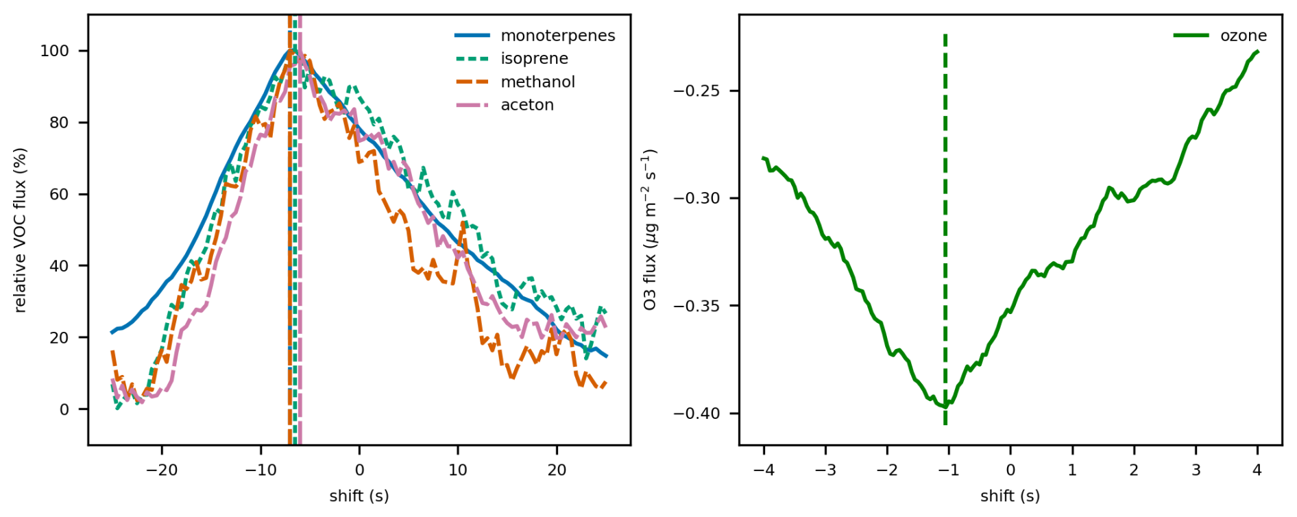
Figure 11VOC (left, 8 July 2023 15:30 CET) and ozone (right, 7 December 2024, 11:30 CET) fluxes calculated for varying delay times between the vertical velocity and concentrations. The vertical dashed lines indicate the time when the maximum absolute flux occurs. The molar masses of the selected VOC's are monoterpenes: 137.132 Th, isoprene: 69.069 Th, methanol: 33.031 Th, acetone: 59.049 Th. For VOCs, the fluxes are normalised by dividing by the maximum absolute flux for that compound.
Second, an important question is if the VOC and ozone concentrations are collected at a sufficiently fast rate, close enough together and with small enough tube damping to not miss the high frequency part of the turbulence spectrum. As a first test, we calculate CO2 fluxes, where we numerically reduce the sample rate from 20 to 0.2 Hz. We do this by applying a block average to the CO2 signal with block widths in a range between 1 and 1000 samples (averaging time s). Note that this represents a worst-case scenario, where we assume that a slower sampling frequency implies longer averaging times instead of less frequently collecting samples with a truly short sample collection time. The results show that applying block averages up to 2 s hardly change the calculated fluxes during this day and in most cases even an averaging time of 4 s still yields similar results as the original (Fig. 12). This shows that, given the roughness of the forest and the high measurement location (38.2 m, 16 m above the canopy), the dominant eddies have a time scale longer than seconds and that the VOC and ozone sample collection frequencies of 2 and 20 Hz are fast enough for calculating turbulent fluxes Faurès et al. (2026), confirm the small impact of frequency corrections over forests. In subsequent analyses of spectra it may be relevant to remember that VOC's and ozone are reactive species, where the complexity of the reactions may affect the mixing lengths and shape of the spectra (Jonker et al., 2004).
We verify this statement by inspecting the power spectra and co-spectra of VOC and ozone concentrations and fluxes (Fig. 13) in relation to those of temperature, water vapour and CO2 measured by the EC system (Sect. 2.5). The shape of the power spectra are as expected (dashed line) for water vapour, while temperature and CO2 concentration are subject to more variance at high frequencies than expected and ozone and particularly VOC concentrations show signs of high frequency noise, Nyquist folding and or low signal to noise ratio. The spectra have a better-defined shape when the fluxes are larger (e.g., T and CO2 in July vs January). In principle, high frequency noise does not necessarily affect the calculated fluxes. Indeed, the co-spectra (bottom row in Fig. 13) show that only waves up to a frequency of about 0.1–0.5 Hz contribute to co-variance. Higher frequency variations in concentrations are not correlated to vertical velocity. This corresponds to the results of our initial block averaging experiment (Fig. 12), which showed that even averaging up to 2–5 s (0.5–0.2 Hz) does not significantly affect the calculated fluxes. Since our EC measurements are sampled at 20 and 2 Hz (Table 7), we are confident that we measure at sufficiently high rates for flux calculations. Nevertheless, the reason behind this high frequency noise should be studied in more detail. For isoprene, methanol and acetone the co-spectra are slightly negative between 0.1 and 1 Hz, the magnitude and shape of these fluxes appear to depend somewhat on the imposed delay time.
The analysis above verifies that the EC measurements of VOCs and ozone are of good quality and can be processed to fluxes. The concentration data will be processed to fluxes similar to the ICOS methodology (Sabbatini et al., 2018; Dumont et al., 2026). Methods of calibrating the absolute concentration, non-linear sensitivity (Muller et al., 2010; Zahn et al., 2012; Dumont et al., 2026) and noise suppression (Aslan et al., 2021) will be described in more detail in future publications. The first version of the ozone concentration and flux data is available as van der Molen et al. (2026j).
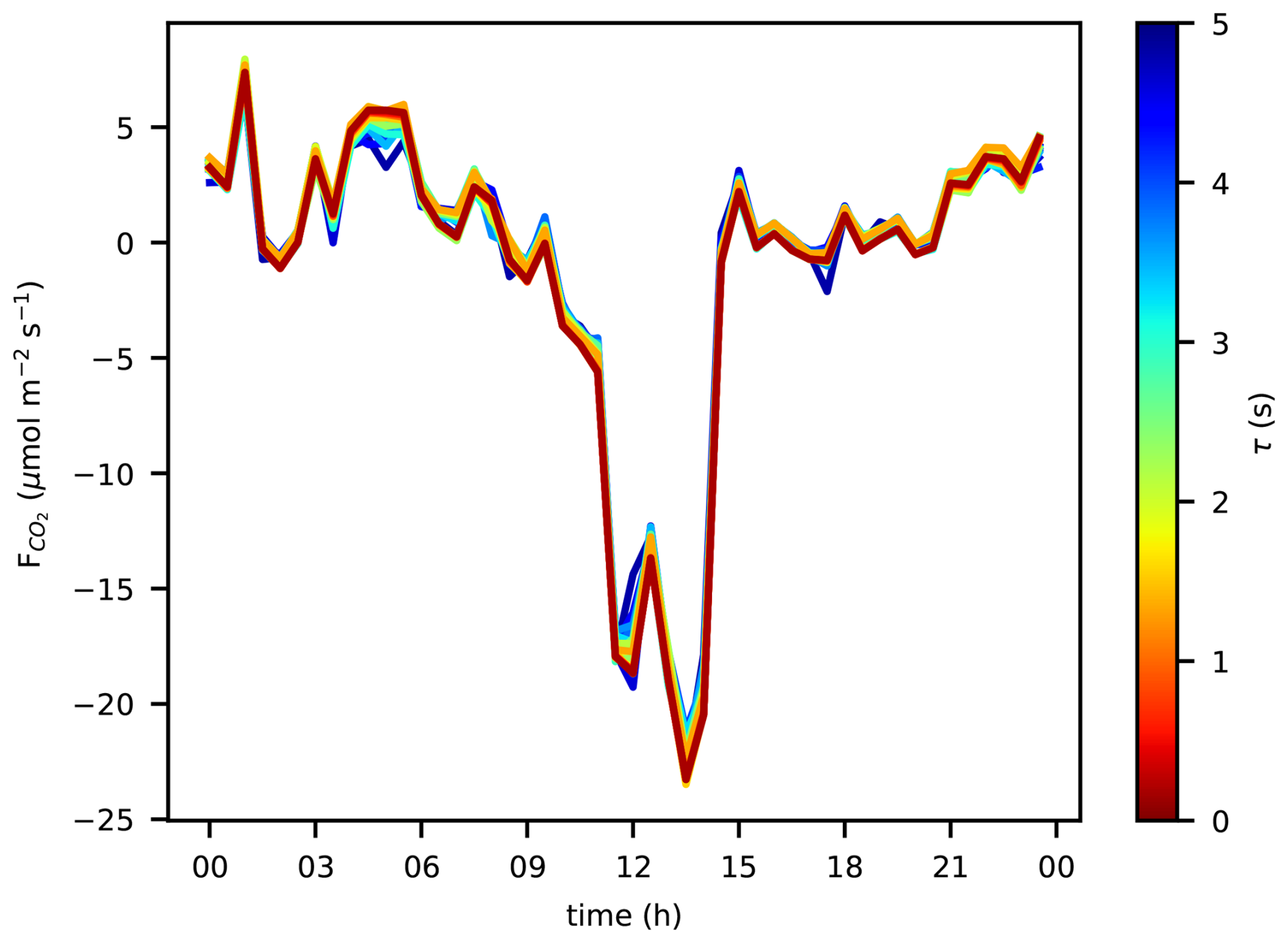
Figure 12Diurnal time series of CO2 fluxes calculated with a block average applied to the CO2 signal with 26 block widths representing an averaging time τ between 0.05 and 5 s. The date is 28 June 2023.
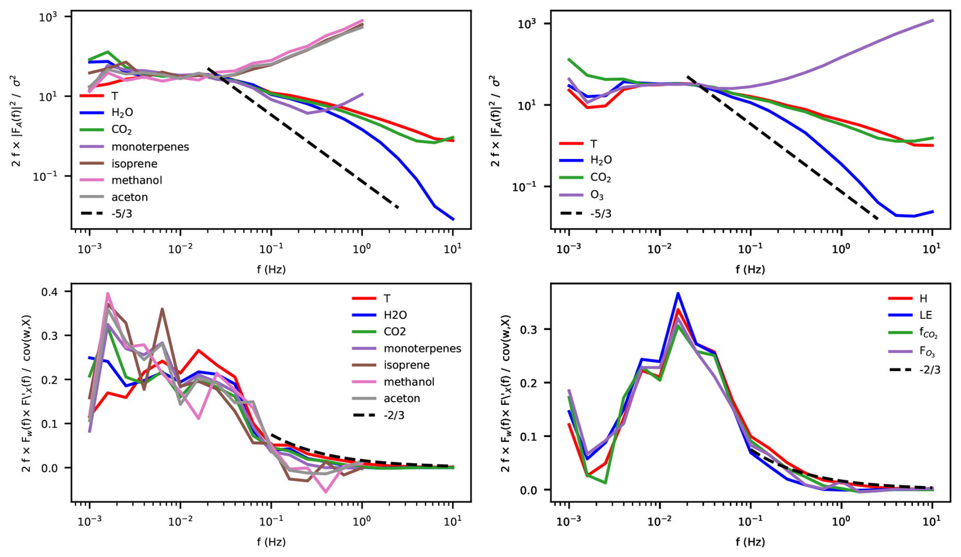
Figure 13Spectra (top) and co-spectra (bottom) of VOCs on 7 July 2023 11:00–13:30 CET (left) and ozone on 17 May 2025 12:00–14:30 CET (right). All (Co)Spectra include temperature (T), water vapor and CO2. The dashed lines show the lines with (top) and (bottom) slopes, along which the spectra would be expected to develop in the inertial subrange.
2.8 Intermittent ecosystem characterisation
2.8.1 Digital Hemispheric Photography
To measure spatial and temporal variability in Green Area Index, digital hemispheric photographs (DHP) are taken. At the continuous measurement plots (CP's) photographs are taken every second month in a 9 point raster. At the 20 SP's photographs were taken once in a 5 point raster (Fig. S2 in the Supplement). The pictures are taken in conditions without direct sunlight, without rain or snow in the air or on the branches and leaves, not close to stems, branches or leaves. A Canon EOS 700D camera with a Sigma 4.5 lens with aperture F8, ISO 200 and shutter time < s was used, which was installed level using a tripod. The photographs are stored in CR2 format, uploaded to ICOS and automatically processed. The procedure is explained in more detail in the ICOS Ecosystem Thematic Centre (ETC) “Instructions for ancillary vegetation measurements in forest” (Gielen et al., 2017). For the first year's results (Summer 2023–Summer 2024), the LAI is estimated to vary between 2.2 and 2.8 m2 m−2 , which is considerably larger than the earlier estimates (Figs. 5 and 6 in Zhao et al., 2026) using a Li_Cor LAI-2000 sensor. To explain this difference, the earlier measurements will be repeated with the original instrument at the original locations and the DHP locations.
2.8.2 Leaf area and nutrient content
Each winter, needles are collected for foliar analysis. In each CP the 6 trees with the largest diameter are selected. From each of these trees, 2 or 3 twigs of the current year's cohort are collected, 30 in total. From 10 needles of each twig, the leaf area is measured with a flatbed scanner. Leaf mass is measured after oven drying the needles at 65 °C for 48 h using a microscale.
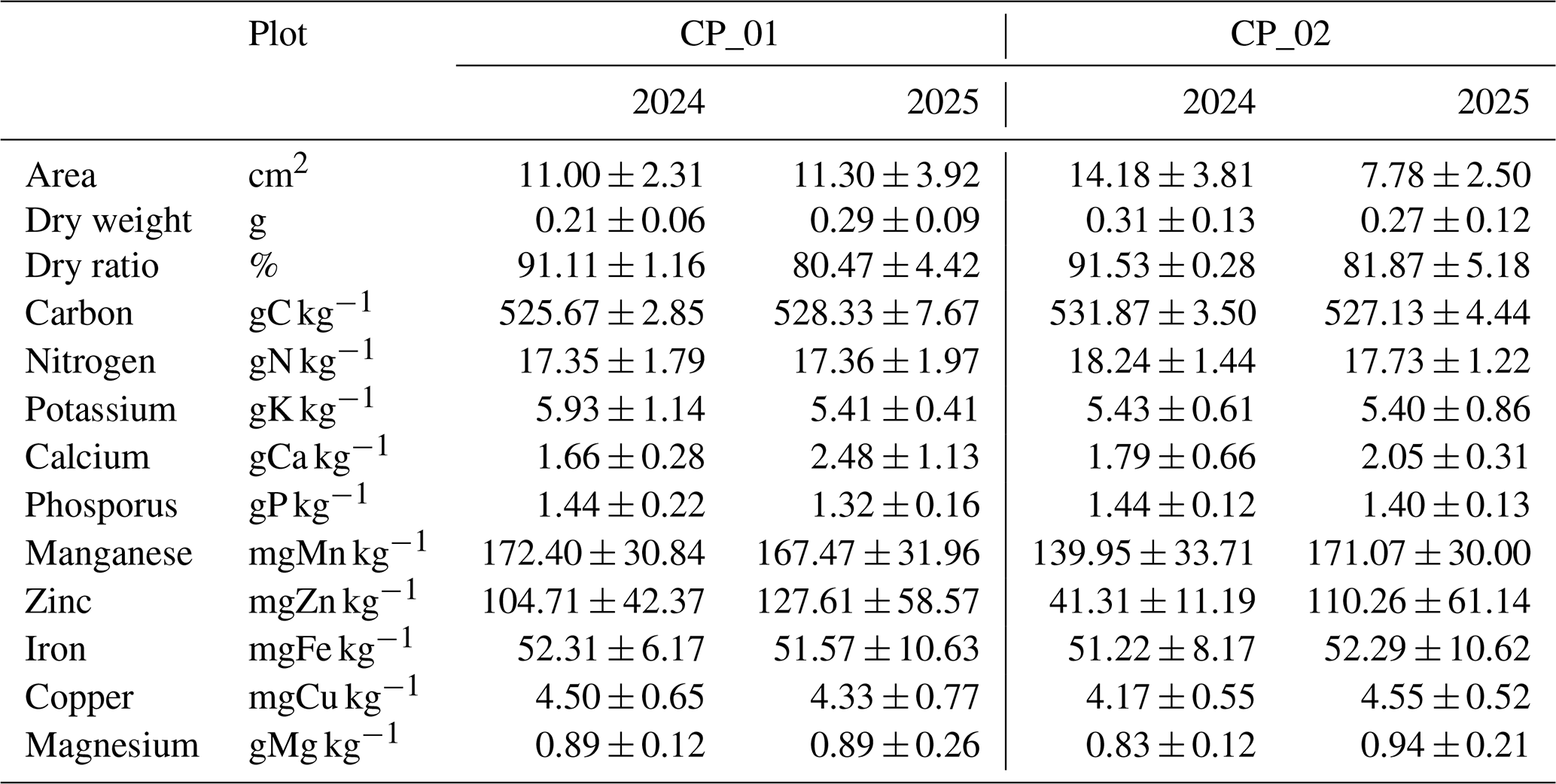
From the same twigs, 20–30 g of needles are collected, dried at room temperature for 2–3 d and send to the ICOS Central Plant Analysis Laboratory, Villenave d'Ornon, France, for nutrient analysis, including N, C, P, K, Ca, Mg, Cu, Fe, Mn and Zn concentrations. Here we follow the ICOS ETC `instructions for foliar samples collection and leaf mass to area ratio determination' (Loustau et al., 2017). The results of the 2024 and 2025 campaign are listed in Table 10. The area, dry weight and C, N and P concentrations shown in Table 10 are in line with sampling campaigns performed in 1998, 1999, 2000, 2003 and 2012 (Table 7 in Zhao et al., 2026), although the variability between years is significant.
Table 10Mass, area and nutrient concentrations of foliar samples in 2024 and 2025. In each Continuous Plots 15 foliar samples were collected from 6 trees (in total 30 samples in two CP's). Each sample consists of 10 needles. The samples were dry weighed at 65 °C, the area measured, then submitted to the ICOS lab in France, where they were dried at 103 °C and analysed for nutrient concentrations. The samples were collected in March 2024/2025. The area and dry mass refer to the total over the 10 needles in a sample. The dry ratio is the ratio of mass at 103 °C and at 65 °C. The mean and standard deviation are calculated over the 15 samples per CP.
2.8.3 Soil inventory
A soil inventory was carried out in Spring 2024 as part of the standard ICOS procedure. At each of the 20 SP's, 5 locations were randomly assigned, 100 in total. At each location, first the organic layer was collected from a 25 × 25 cm area. Then an 8 cm diameter 100 cm deep soil core was taken. The core was divided into 5 sections: 0–5, 5–15, 15–30, 30–60 and 60–100 cm. Photographs were taken from the core and/or a soil pit. The soil in each section was collected in a plastic bag. The samples were fresh weighed, dried, dry weighed, split into dead and life biomass (organic samples) and mineral soil and plant residue (mineral samples) to determine soil dry bulk density. The 600 samples have been sent to the ICOS ETC European Soil Samples Conservatory in Orléans, France to be analysed for soil organic carbon and nitrogen content. A more detailed description of the procedure can be found in the ICOS ETC Instructions for soil sampling and preparation (ICOS ETC, 2026). The results of the 2024 campaign are not available yet. The soil inventory will be repeated with a 10-year interval.
2.9 Measurement campaigns and experiments
The renewed and extended infrastructure has been home to several intensive field campaigns and experiments. On 17–18 May 2022, an extensive campaign was held within the Ruisdael Observatory project (https://ruisdael-observatory.nl/, last access: 4 February 2026). The aim was a characterization of the vertical and horizontal variability of meteorology and atmospheric constituents between grassland (Cabauw site) and the Loobos forest site. Besides the regular measurements, radio soundings were released to measure profiles of temperature, humidity and wind speed and direction. An aircraft (Sun et al., 2023) was flown over the area several times per day to measure temperature, humidity, CO2 concentration at a high frequency (50 Hz), which enabled the calculation of turbulent fluxes at different levels in the atmospheric boundary layer. Flasks were filled with air to be analysed for δ() ratio, CO, COS, CH4, and the stable isotope concentrations δ13C in CO2 and δ18O in H2O. Manual measurements were performed at leaf level to measure photosynthesis rates and surface conductance. These data have been analysed for the relative contribution of surface and atmospheric signals, placing special emphasis on the individual contributions of processes that control the boundary layer development dynamics (Faassen et al., 2025).
The Loobos forest is immediately downwind from an area of major agricultural ammonia emissions. During two separate periods, an HT8700 open path ammonia analyser (Healthy Photon, inc.) was installed in combination with a miniDOAS to measure variations in NH3 concentration and its absolute concentration. The experiment was held to test the setup, its applicability for eddy covariance flux calculations and if the setup could be installed operationally. The experiment and results are described in a paper by Melman et al. (2026).
A collaborative group consisting of researchers from Helmholtz Centre Potsdam, GFZ German Research Centre for Geosciences, TU Delft, Department of Geoscience and Remote Sensing, and University of Twente, ITC installed global navigation satellite system (GNSS) sensors at the top of the tower and at 5 locations underneath the canopy in an experiment to measure Vegetation Optical Depth (VOD). The data collection, analysis and verification is ongoing. GNSS data from GFZ systems is available upon request to Benjamin Brede (Contact: https://www.gfz.de/en/staff/benjamin.brede/sec14, last access: 13 October 2026).
On 28 August 2024, a multi-scale experiment was performed using ground observations of Sun Induced Fluorences (SIF, ESA FloX), CO2 fluxes and 10 Hz multiband incoming and outgoing radiation intensities installed at 8 different levels in the tower, an airborne Flying Laboratory of Imaging Systems (HyPlant and CzechGlobe), consisting of hyperspectral sensors CASI-1500, SASI-600 and TASI-600, and a LMS Q780 airborne full-waveform laser scanner. The measurement suite is complemented with TROPOMI satellite retrievals of SIF (Köhler et al., 2018). The purpose is to compare the retrieved data at different scales to work towards better understanding of ground, airborne and satellite observed data. Data inquiries via the corresponding authors.
A distributed temperature sensing (DTS) system is employed by the Civil Engineering & Geosciences, Water Resources group of Delft University of Technology (Schilperoort et al., 2024). Currently, the system aims at experimentally measuring dry and wet bulb temperatures along the tower in order to better understand transpiration and evaporation. Contact: Miriam Coenders (https://www.tudelft.nl/staff/a.m.j.coenders/, last access: 13 October 2026).
In this section, we demonstrate some of the capabilities of the station to measure the CO2 fluxes. Section 3.1 shows how the total CO2 flux is composed of a turbulent flux and a storage flux, and how the distribution over the two depends on the degree of turbulence. Section 3.2 shows how the CO2 fluxes measured in the second tower (described in this paper) compare with the fluxes measured in the first tower (Zhao et al., 2026).
3.1 Distribution over turbulent and storage fluxes
The CO2 flux measurements are composed of an eddy covariance part (Sect. 2.5) and a storage fluxes part (Sect. 2.6). Here we test if the combination of those systems is well-capable to measure the total flux. As mentioned, in sufficiently turbulent conditions, the entire flux is measured by the eddy covariance system, because the below canopy air is well-mixed with the surface layer, this is confirmed in Fig. 14 below. In conditions with low turbulence intensity, such as may occur in calm, stable nights, the CO2 respired from the ecosystem is hardly mixed to above canopy air and accumulates in the air below the canopy. We demonstrate this behaviour in Fig. 14 or three nights in a row in September 2024, when the first night is very turbulent, the second night medium turbulent and the third night calm. The air temperatures are roughly similar each night, although the first night 1–2 °C colder than the other two.
In daytime conditions, the CO2 gradient is typically less than 10 ppm from the top of the tower down to the forest floor. In the first night, the CO2 profile is still relatively well mixed, m s−1 and the atmosphere only slightly stable with .1–0.2 (both u* and are derived from the eddy covariance measurements at 38.2 m). The CO2 gradient between the lowest (0.1 m) and second (0.4 m) is about 10 ppm and the gradient from 0.4 m to the top of the tower (38.2 m) is another 10 ppm. Hence, there is hardly any accumulation of CO2 below the canopy. Hence the storage flux is close to 0 and the autotrophic and heterotrophic CO2 respiration flux is properly measured by the eddy covariance system (about 5 µmol m−2 s−1).
In the second night, turbulence intensity decreases, u* decreases from 0.4 to 0.15 m s−1 and increases from 0.1 to > 0.5. The turbulence is not sufficiently strong to mix all of the respired CO2 to above the canopy. The CO2 gradient is 120 ppm at the end of the night, with the average vertical 17 ppm per level between the surface and 11.2 m high, which, incidentally, shows that the height of the levels is well-chosen. Between 15.7 and 38.2 m the total gradient is 5 ppm, which suggests that the gradient is built up from the soil surface upward. In this situation, the total flux is a mix of eddy covariance flux and storage flux, and the sum of both terms is roughly equal to the 5 µmol m−2 s−1 measured in the night before.
In the third night, the turbulence intensity is even smaller, m s−1 until 06:00 in the morning, when it increases. The stability is expressed by in the evening and early night, afterwards it becomes unreliable under influence of small fluxes. The CO2 strongly accumulates in the below canopy air, with the highest concentrations (730 ppm) near the ground, a total gradient of 230 ppm, which is distributed nearly even over the levels (∼ 23 ppm level−1), although the 15.7 m level exhibits concentrations closer to the 22.1 m level, suggesting respiration from the canopy crown contributes to CO2 accumulation too. In this situation, the eddy covariance flux is indeed 0 and the total respiration – again roughly 5 µmol m−2 s−1 – is entirely represented by the storage flux. The onset of turbulence is at 06:00 in the morning, when the storage flux becomes negative (depletion of CO2) and the eddy covariance flux becomes positive (upward flux). Later in the morning, photosynthesis becomes an important term. Interestingly, complete removal of the stored CO2 below the canopy by photosynthesis takes until 09:00 in the morning, three hours after the onset of mixing at 06:00. This figure also indicates that the below canopy air returns to well-mixed conditions at daytime again. Hence, ignoring the storage flux will not affect the daily total fluxes measured by the eddy covariance system, but it will affect its distribution over the day. Note that u* filtering would flag most of the nocturnal data, particulary in the 3rd night.
The above shows that the profile system is capable of measuring the buildup of vertical gradients below the eddy covariance system, thus complementing each other for the purpose of measuring the total CO2 flux. However, horizontal advective fluxes may disturb the relation between the buildup of vertical gradients and the actual respiration flux. We did not measure advective fluxes, but it may be interesting to inspect the horizontal wind speeds above and below the canopy. In the first night, the windspeed at 38.2 m is 3.5 ± 1 m s−1, 1.5 m s−1 at 22.1 m (canopy level), decreasing to below 1 m s−1. Below the canopy, the windspeeds are 0.5 m s−1 or lower. In the second night, the 38.2 m windspeed decreases from 4 to 2 m s−1, the 22.1 m windspeed decreases from 1 to 0.5 m s−1 and the below canopy windspeeds decrease from 0.5 to below 0.2 m s−1. In the third night, the 38.2 m windspeed is intermittently between 0.5 and 1.0 m s−1 and between 1 and 2.5 m s−1. The windspeeds at 22.1 and below are mostly in the order of 0.1 m s−1, although the 22.1 m windspeed sometimes increases with the 38.2 m windspeed.
It appears that only in more calm and stable conditions, the windspeeds drop considerably below 1 m s−1, in less calm nights the windspeed could be large enough to cause horizontal CO2 advection. With a distance of 1.8 km to the nearest edge of the (spatially quite homogeneous) forest and a windspeed of 1 m s−1, it would take 30 min for the wind to move from the forest edge to the station, during which horizontal gradients induced by the transition to forest may not be entirely settled. So, although there is no indication of an imbalance of the sum of turbulent and storage flux and the expected total flux of 5 µmol m−2 s−1, we cannot guarantee that advective fluxes are absent at the site.
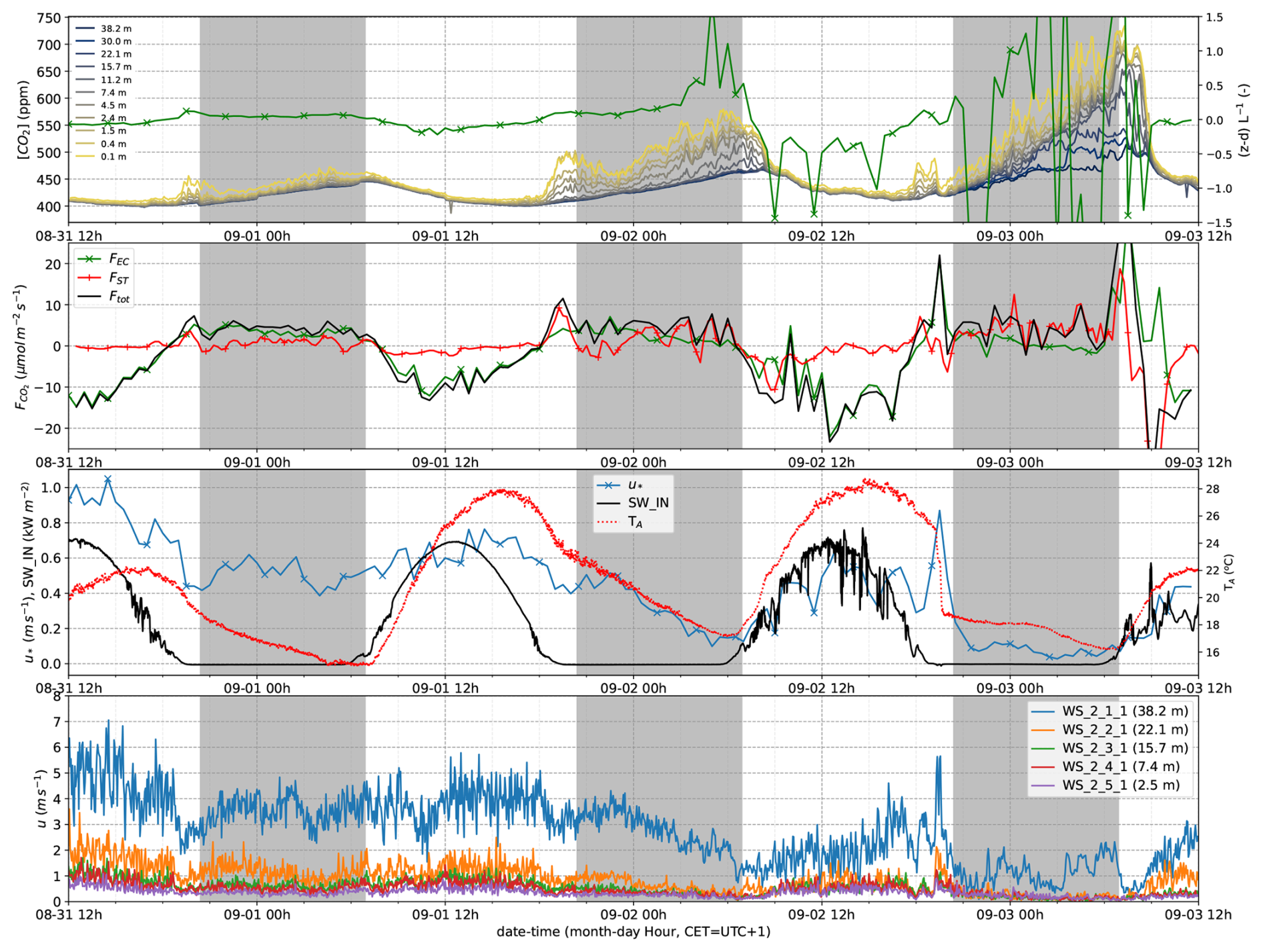
Figure 14Top: CO2 concentrations measured in the profile along the tower. Second: Eddy covariance flux, storage flux and total flux (NEE). Here we show the eddy covariance fluxes without post-processing (u* filtering and gapfilling) as output from EddyPro. Third, left axis: u* and incoming shortwave radiation, right axis: air temperature at 2.4 m. Bottom: Wind speed profile (3 min block average). These data were measured between 31 August–3 September 2024. The shaded areas represent the time between sunset (20:24 CET) and sunrise (06:54 CET).
3.2 Continuity of NEE timeseries from the first tower to the second
The second tower (since 2021) is intended to continue the first tower measurements (1996–2023) and to build a continuous long-term timeseries. Since the measurement heights and instrumentation (open path and closed path gas analyser) were different, it is relevant to verify if the fluxes measured by the systems in the two towers match. Unfortunately, the gas analyser in the first tower suffered a breakdown for a long period after the second tower's eddy covariance system was installed. However, we do have a 2 month period of overlapping data in between 28 July–29 September 2021. Despite a small distance (< 20 m) between the two towers, the flux footprints of the two towers overlap and cover the same vegetation type. The total ecosystem respiration does not vary with footprint distance (Fig. 18). Figure 15 shows the level to which the two datasets agree. The diurnal cycles show much agreement in the four days shown, even at nighttime, when below sensor storage could be different for the two systems. With a r2 of 0.74 there is some random variability between the datasets, but the slope is close to 1 and the offset small relative to the magnitude of the fluxes. Quality flags quantify the quality of the flux data (Vitale et al., 2000). Here only data with quality flag 0 have been selected, representing the best quality data. Selecting data with quality flags 1 and/or 2 will result in a significantly worse match. Since the second tower was not yet labelled as an ICOS site, we use our own EddyPro results in this comparison. Figure S3 in the Supplement, however, shows that there is a near 1:1 correspondence between our own EddyPro calculations and the ICOS ETC L2 and Near Real Time (NRT) results. Differences could occur due to differences between sensors, different heights of the sensors, affecting flux footprint, frequency corrections, and different flux processing.
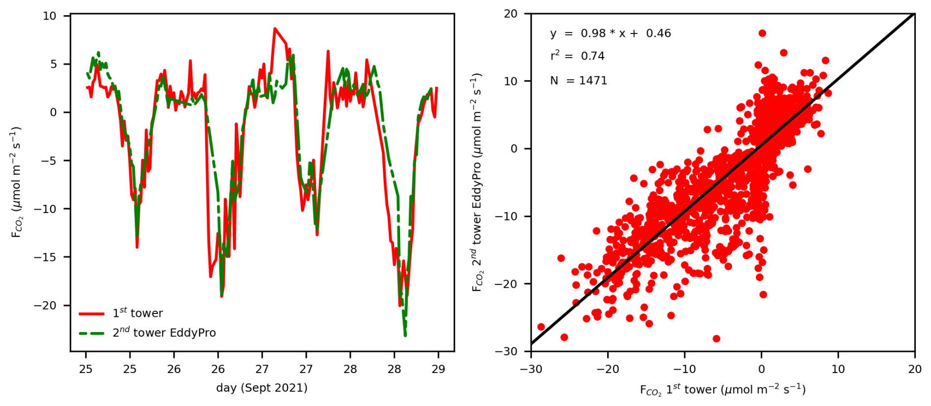
Figure 15Comparison of the eddy covariance CO2 fluxes measured by the first tower (Zhao et al., 2026) and the second tower. Left: the diurnal cycles over a subset of the two month period. Right: the correlation between the two datasets. Here only data with quality flag 0 have been selected.
Looking at a longer timescale, van der Molen et al. (2026k, Fig. 1), however, show a discontinuity in monthly mean total ecosystem respiration around the time of the transition from the first to the second tower. In the supporting information, they attempt to explain the discontinuity by (1) a change in eddy size distribution with increasing the measurement height from z = 27 m to z = 38.2 m (In the first tower, z−d changes from 16.8 m in 1997 to 13.5 m in 2021, in the second tower z−d is 24.7 m, where d is the zero-plane displacement height, taken as rd of the canopy height): the frequency loss correction factors are only in the order of max 4 % for m s−1 (Fig. 16) and hence cannot explain the larger discontinuity; (2) by a change in flux footprint: the footprint is homogeneous (Fig. 9, Sect. 1.2) and the respiration rate does not depend on footprint size (see Fig. 18); or by (3) a change in effective threshold u* value with decreasing effective measurement height: implementing a variable threshold value does not change the fluxes considerably. Their conclusion is that they cannot yet explain the discontinuity with the second tower's dataset still too short to know if the observed trend continues.
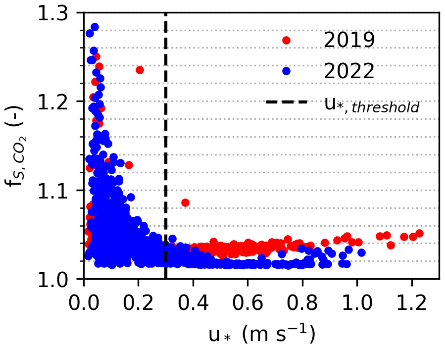
Figure 16Spectral correction factors for nighttime CO2-fluxes as a function of u*, measured at 23 m in 2019 (on top of the first tower) and at 38.2 m in 2022 (on top of the second tower), both with the second tower's eddy covariance setup. In both years we used data in June and July. The vertical dashed line indicates the u* threshold value.
Interestingly, from 15 May–7 September 2019, before we built the second tower, we did a test run of the new tower's eddy covariance system in the first tower, alongside the first tower's own eddy covariance setup (Zhao et al., 2026). Both systems were installed at a height of 27 m, within 2.5 m from each other. In Fig. 17, we show three hourly mean fluxes with selection criteria qc_co2_flag = 0 or 1 (best), m s−1, global radiation >10 W m−2 for daytime and <2.0 W m−2 for nighttime data. Although not too many half hours pass the selection criteria, the agreement between the two measurement systems is satisfactory. Confusingly, the 2nd system now has somewhat smaller fluxes than the 1st tower system (as opposed to Fig. 1 in van der Molen et al., 2026k).
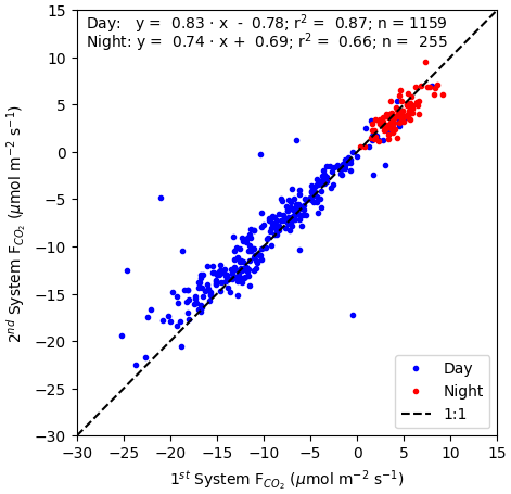
Figure 17Comparison of CO2 fluxes measured at the top of the first Loobos tower (27 m), with the 1st tower's eddy covariance system (x-axis) and the 2nd tower's eddy covariance system (y-axis), between 15 May–7 September 2019 with selection criteria qc_co2_flag = 0 or 1 (best), m s−1, global radiation >10 W m−2 for daytime and <2.0 W m−2 for nighttime data.
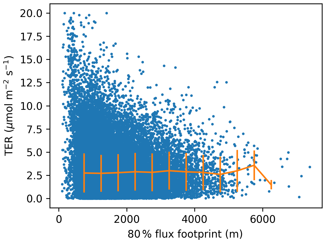
Figure 18Total Ecosystem Respiration (TER) as a function of flux footprint distance in the second tower. The orange line with errorbars indicates the mean and standard deviation. Although the apparent variability in TER is larger with smaller footprint size, the mean and standard deviation are constant, because there are more data points at smaller distances.
In addition to the trends in TER (van der Molen et al., 2026k, Fig. 1), we show the corresponding trend in Gross Primary Production (GPP, Fig. 19). The discontinuity observed in TER is not visible in GPP. A positive trend is visible in GPP, particularly in fall. GPP is clearly lower in the dry years 2003, 2013 and 2018. Figure 20 shows the corresponding trends in latent heat flux (LE). Here again a discontinuity is observed after the transition to the second tower.
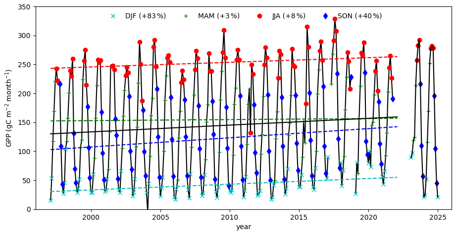
Figure 19Trend in GPP per season. The markers show monthly sums. The colours combine the months into seasons as indicated in the text within the figure. The dashed lines indicate the linear regression lines of seasonally mean GPP. The percentages shown in the legend indicate the change in GPP from 1997 to 2021 relative to 1997. From 1997 to 2021, the GPP from NEE partitioning is shown (Zhao et al., 2026). The post 2021 data represent GPP from the ICOS FLUXNET half-hourly product from 2023 to 2024 (van der Molen et al., 2026l).
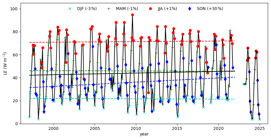
Figure 20Trend in Latent Heat flux (LE) per season. The markers show monthly means. The colours combine the months into seasons as indicated in the text within the figure. The dashed lines indicate the linear regression lines of seasonally mean LE. The percentages shown in the legend indicate the change in LE from 1997 to 2021 relative to 1997. From 1997 to 2021, the gapfilled LE from Zhao et al., 2026) is shown. The post 2021 data represent LE (LE_F_MDS) from the ICOS FLUXNET half-hourly product from 2023 to 2024 (van der Molen et al., 2026l).
These results combined suggest that the flux measurements of the first and second tower correspond to a high degree when comparing half-hourly data, but when looking at long-term trends, additional work is necessary to explain apparent discontinuities in TER and LE. It is interesting to note that Jung et al. (2024) detected long-term discontinutities in NEE and LE for 20 %–25 % of the sites in FLUXNET. They carefully point towards instrumentation changes if ecosystem disturbances cannot explain the discontinuity.
The data collected with the infrastructure we describe in this paper are available for interested people via a CC-BY-4.0 license. We distinguish data collected according to ICOS instructions and non-ICOS data.
The ICOS data are
-
the radiation data described in Sect. 2.2. Note that the Phenocam data are available via the NAU Phenocam Network site until May 2026 and via the ICOS Carbon Portal afterwards;
-
the continuous soil measurements in Sect. 2.3;
-
the precipitation, air pressure, temperature, humidity and backup measurements (Sect. 2.4);
-
The ICOS compliant eddy covariance measurements of CO2 and H2O (Sect. 2.5);
-
The vertical profiles of CO2, H2O and temperature and windspeed (Sect. 2.6), except the leaf wetness data;
-
The intermittent ecosystem measurements (Sect. 2.8);
All ICOS data are available via the ICOS Carbon Portal (https://www.icos-cp.eu, last access: 13 October 2026), more specifically the Loobos ecosystem site's page https://meta.icos-cp.eu/resources/stations/ES_NL-Loo (last access: 13 October 2026). In general, ICOS publishes
-
level 0 data: the raw data we submitted,
-
level 1 data: The Near-Real Time (NRT) data, which represents intermediate observational data, quality controlled and updated on a daily basis
-
level 2 data: the final quality observational controlled data. Level 2 data are updated on an annual basis.
ICOS offers downloads for all data and previews of key variables in the level 1 and 2 data.
Our own https://MAQ-Observations.nl (last access: 4 February 2026) offers download and visualisation of the ICOS level 0 data, including eddy covariance fluxes processed with EddyPro. Additionally, it provides the vertical profile leaf wetness data (Sect. 2.6).
Other non-ICOS data include the ozone and VOC concentration and flux data and NO2 concentration concentration data. The processed ozone concentration and flux data are available via https://doi.org/10.17887/WUR01-6UGU9F (van der Molen et al., 2026j) and will be updated on an annual basis. The VOC data will be made available via the same yoda.wur.nl platform as the ozone data. Raw (20 Hz) ozone and VOC data and all other data not (yet) available via the ICOS Carbon Portal or MAQ-Observations.nl is available upon request via the authors.
In general, we advice to download data preferably from the ICOS Carbon Portal as level 2 data if available, otherwise as level 1 data or level 0 data, because ICOS offers high-quality quality control and gap filling and provides persistent data identifiers.
All data described in Sect. 2.2–2.4 and 2.6 are uploaded to https://MAQ-Observations.nl (last access: 4 February 2026) every 30 min and to the ICOS Carbon Portal (2026) on a daily basis. Our data is available in near real-time, including customizable charts, at MAQ-Observations. The data are available for use according to a CC-BY 4.0 data licence. Any used data must be cited accordingly, please refer to https://maq-observations.nl/maq-data-license/ (last access: 4 February 2026) and https://www.icos-cp.eu/how-to-cite (last access: 4 February 2026). On the ICOS Carbon Portal we recommend to look for the L2 product for previous years and to the Near-Real-Time (NRT) data product for the ongoing year. The PhenoCam data are accessible via https://phenocam.nau.edu/webcam/sites/nlloobs/ (last access: 4 February 2026). All data described in other sections are available for use according to the same licenses too, please contact the authors of this paper to obtain access.
ICOS Level 2 (L2) products can be downloaded via the ICOS Carbon Portal:
-
ETC L2 Archive from Loobos 2023-01-01–2025-10-01, DOI: https://doi.org/11676/RBbGtSvPuyjgktNpRDUq5fpw (van der Molen et al., 2026a)
-
ETC L2 Meteosens from Loobos 2022-12-31–2025-09-30: DOI: https://doi.org/11676/ue7IUwhI1eSbNEsFZtbvWjur (van der Molen et al., 2026b)
-
ETC L2 Meteo from Loobos 2022-12-31–2025-09-30, DOI: https://doi.org/11676/7OvfpkiXvumy_vSHQ6ds3Zbo (van der Molen et al., 2026c)
-
ETC L2 Fluxes from Loobos 2022-12-31–2025-09-30, DOI: https://doi.org/11676/Ww4zYPNKHkBUcjZxNS4CXN1j (van der Molen et al., 2026d)
-
ETC L2 Auxdata from Loobos 2023-05-10–2025-10-01, DOI: https://doi.org/11676/N3zBxhFvmOdlkXIW8jwryl-A (van der Molen et al., 2026e)
ICOS Near Realtime Observational Data (NRT, Level 1) can be downloaded via the ICOS Carbon Portal:
-
ETC NRT Meteosens from Loobos, 2025-09-30–2026-10-13, DOI: https://doi.org/11676/vht9qQfacM_WjZ24HUnUjOhJ (van der Molen et al., 2026f)
-
ETC NRT Meteo from Loobos, 2025-09-30–202610-13, DOI: https://doi.org/11676/TDS7X7R-Uoubk21p19vLGkP8 (van der Molen et al., 2026g)
-
ETC NRT Fluxes from Loobos, 2025-09-30–2026-10-13, DOI: https://doi.org/11676/76WMKzUWq6oHD8qiwAs1sL1h (van der Molen et al., 2026h)
-
DOI: ETC NRT AuxData from Loobos, 2025-09-30–2026-10-13, https://doi.org/11676/jP_yJ8wTKCcVQkJMzqAHlt5O (van der Molen et al., 2026i)
-
ICOS Forest ancillary data are available via: https://icos.uantwerpen.be/Content/AncillaryReports/NL-Loo_Ancillary_Report.html (Iserbyt et al., 2026) (will be merged with ICOS-cp.eu)
-
The Ozone concentration and flux data will be published as annual archives. The 2025 data are available via https://doi.org/10.17887/WUR01-6UGU9F (van der Molen et al., 2026j). Intermediate data are available upon request.
The Python codes for processing the data and plotting Figs. 9, 11–15 and S.3 can be found at https://git.wur.nl/molen050/loobos-second-tower-reference-paper (last access: 13 October 2026).
With the infrastructure and instruments outlined in this paper, we aim to establish Loobos as a flagship site within the international scientific community, a forefront ecosystem site for long-term, interdisciplinary ecosystem and atmospheric research. Our ambition is to contribute cutting-edge data and insights that inform both science and policy at national and global scales.
-
Advancing Carbon Cycle Science. The installation of a second flux tower at Loobos marks a major step toward its labelling as an ICOS Class 2 Ecosystem Station. This enables us to extend the long-term carbon sequestration record initiated in 1996 (Zhao et al., 2026), capturing the forest's response to gradual, abrupt, and intermittent climate variability – including heatwaves, droughts, and pollution episodes. The combination of flux measurements and vegetation characterisation makes a significant contribution to the advance of carbon cycle science. Our data feed into the ICOS Carbon Portal, supporting a wide range of continental and global carbon budget assessments. Being part of an international infrastructure will increase the station's visibility and facilitate our ambitions by providing robustness, standardisation, a long-term horizon and international collaboration. We are in the process of collecting a long-term dataset. An example of its analysis can be found in van der Molen et al. (2026k) who analyse the long-term trend in total ecosystem respiration.
-
Linking Air Quality and Ecosystem Functioning. By integrating measurements of VOCs, NOx, O3, and NH3, we investigate how fertilization, acidification and air pollution influence carbon uptake and forest health. Loobos is uniquely positioned downwind of one of the world's largest nitrogen-emitting regions, making it an ideal site to monitor the effects of evolving emission policies. Together with ICOS stations in Cabauw and Lutjewad, Loobos forms a strategic transect for studying sectoral emission impacts. We have installed instrumentation for O3 and VOC fluxes and are in the process of developing operational data processing tools. Ammonia fluxes were experimentally measured from 24 August 2023–5 September 2024, which resulted in a much higher estimate of the deposition rate (Melman et al., 2026). We are applying for funding to measure NH3 and NOx fluxes on an operational basis to establish a timeseries quantifying the effect of expected nitrogen emission policy changes and to provide data needed for improvements of deposition models. A PhD position starts in August 2026 to explore microplastics concentration and flux measurements. A fast response Portable Optical Particle Spectrometer (POPS) particulate matter sensor is on loan from Delphine Farmer (Colorado State University).
-
Quantifying Forest Water Dynamics. We are measuring the forest's water consumption and yield to address growing concerns about hydrological imbalances in the Veluwe region, a critical source of drinking water. Our observations will provide a scientific foundation for advising policymakers on the role of forest type and management in sustainable water harvesting. We are currently partner in the public-private “Recharge” project (https://tki-recharge.nl/, last access: 13 October 2026) with drinking water companies and water authorities to study groundwater recharge in the Veluwe area and the relation with climate and ecosystem types.
-
Enabling Fundamental Ecosystem-Atmosphere Research. Loobos serves as a platform for advanced research into canopy-atmosphere exchange processes. Faassen et al. (2025) show how boundary layer concentrations are affected by the interaction of surface and entrainment fluxes. Understanding the interactions between canopy processes and boundary layer dynamics is essential for improving weather and climate models, especially those incorporating dynamic vegetation (Boussetta et al., 2013). We aim to deepen our understanding of radiation, heat, water, momentum, and trace gas fluxes – particularly the role of in-canopy gradients in shaping photosynthesis, stomatal behaviour, and deposition dynamics.
Our goal is to generate comprehensive datasets for validating next-generation multi-layer canopy models, including large-eddy simulations of turbulent exchange (Pedruzo-Bagozfgoitia et al., 2023) and the MLC-CHEM model (Ganzeveld et al., 2002; Visser et al., 2022). The observations and model development will be (partly) supported by the Ruisdael Observatory Virtuel Research Environment (ROVRE) awarded by NWO (2026b).
-
Supporting Satellite and Aircraft Observations. Loobos plays a key role in satellite retrieval validation, in synergy with the Ruisdael/WUR research aircraft (PH-WUR), enhancing the accuracy of remote sensing products. We are a partner in the recently awarded ASCENT project (Advancing hyperSpectral imaging for Cross-scale Ecosystem fuNctioning and vegeTation research, NWO, 2026c), where a consortium of Dutch universities will measure and upscale hyperspectral data, such as Sun-Induced-Fluoresence radiation on leaf, ecosystem and regional scales. Loobos, as an ICOS station, also plays its role as ground truth in regional remote sensing studies, such as the NUBICOS associated to ICOS (ICOS Carbon Portal, 2026).
-
Experimental DTS setup. The infrastructure is attractive to test experimental setups, such as the Distributed Temperature Sensing setup, installed by Delft University (Miriam Coenders and Gijs Vis). We are applying for funding to enhance our activities in this field.
-
Hosting Targeted Field Campaigns. With its extensive infrastructure, Loobos is a prime location for field campaigns focused on boundary layer exchange and remote sensing calibration. Recent and ongoing campaigns include the canopy – boundary layer exchange experiment (Faassen et al., 2025), a 2024 HyPlant mission and GNSS studies by Delft, Twente, and Potsdam Universities.
-
Fostering Interdisciplinary Collaboration. Loobos brings together expertise from carbon cycle science, hydrology, ecology, soil science, forestry, meteorology, and air quality. This interdisciplinary approach is vital for understanding ecosystem services – such as carbon storage, water regulation, and biodiversity – under increasing anthropogenic pressure and climate change.
The supplement related to this article is available online at https://doi.org/10.5194/essd-18-8637-2026-supplement.
MvdM is the station PI. He conceptualized the study and wrote the manuscript. HS is the station technician, he conducted sampling, collected the manual data and maintained the site. RH, JF and LG is responsible for the VOC, ozone and NO2 measurements, JB and HZ are responsible for data storage, data processing and data verification. WP, MK, JV, LG and BK have been and are responsible for continuity of the station in terms of finances, proposal writing and scientific output. All authors reviewed and revised the manuscript.
The contact author has declared that none of the authors has any competing interests.
Publisher's note: Copernicus Publications remains neutral with regard to jurisdictional claims made in the text, published maps, institutional affiliations, or any other geographical representation in this paper. The authors bear the ultimate responsibility for providing appropriate place names. Views expressed in the text are those of the authors and do not necessarily reflect the views of the publisher.
The station is built on land owned by the Dutch National Forest Service (Staatsbosbeheer). We acknowledge payment of the ICOS station fees by the Ministry of Infrastructure and Water Management.
The PhenoCam was kindly supplied by Yunpeng Luo (Ecosystems Ecology, Forest Dynamics group, Swiss Federal Institute for Forest, Snow and Landscape Research WSL) as part of the Velux project (https://veluxstiftung.ch, last access: 13 October 2026). Data used in this research were provided by the PhenoCam Network, which has been supported by the National Science Foundation, the Long-Term Agroecosystem Research (LTAR) network which is supported by the United States Department of Agriculture (USDA), the U.S. Department of Energy, the U.S. Geological Survey, the Northeastern States Research Cooperative, and the USA National Phenology Network. We thank the PhenoCam Network collaborators, including station PIs and technicians, for publicly sharing the data that were used in this paper.
We acknowledge the help and support from ICOS ETC staff during installation, verification of file formats and data submission. Part of this paper follows the structure of the ICOS ETC Labelling report written for Loobos.
We acknowledge the support of staff and students from Wageningen University during the tree and soil inventory field campaigns and lab analysis.
We thank Roel Dijksma (Hydrology and Environmental Hydraulics, Wageningen University) for explaining the geological history and verifying the description.
We used Microsoft Copilot to help better structure Sect. 4 of the manuscript. We did not use AI to write or rewrite other sections. We take full responsibility for the text in the full manuscript and supplements.
This research has been supported by the Nederlandse Organisatie voor Wetenschappelijk Onderzoek, Exacte en Natuurwetenschappen (Ruisdael Observatory (grant no. 184.034.015)).
This paper was edited by Kirsten Elger and reviewed by Holger Lange and one anonymous referee.
Air Quality Measuring Network: Luchtmeetnet (EN: Air Quality Measuring Network), https://www.luchtmeetnet.nl/meetpunten?station=NL10738&component=O3 (last access: 13 October 2026), 2026.
Aubinet, M., Vesala, T., and Papale, D. (Eds.): Eddy Covariance, Springer Netherlands, Dordrecht, https://doi.org/10.1007/978-94-007-2351-1, 2012.
Aslan, T., Peltola, O., Ibrom, A., Nemitz, E., Rannik, Ü., and Mammarella, I.: The high-frequency response correction of eddy covariance fluxes – Part 2: An experimental approach for analysing noisy measurements of small fluxes, Atmos. Meas. Tech., 14, 5089–5106, https://doi.org/10.5194/amt-14-5089-2021, 2021.
Bakker, M. A. J. and van der Meer, J. J. M.: Structure of a Pleistocene push moraine revealed by GPR: the eastern Veluwe Ridge, The Netherlands, Geol. Soc. Lond. Spec. Publ., 211, 143–151, https://doi.org/10.1144/GSL.SP.2001.211.01.12, 2023.
Benneth, M. R.: The morphology, structural evolution and significance of push moraines, Earth Sci. Rev., 53, 197–236, https://doi.org/10.1016/S0012-8252(00)00039-8, 2001.
Berg, M. W. and Beets, D. J.: Saalian glacial deposits and morphology in the Netherlands, in: Tills and Glaciotectonics, Balkema, Rotterdam, 223–251, ISBN 90-6191-731-0, https://www.dehondsrug.nl/wp-content/uploads/2022/01/VandenBergBeets1987.pdf (last access: 26 October 2026), 1987.
Boussetta, S., Balsamo, G., Beljaars, A., Panareda, A.-A., Calvet, J.-C., Jacobs, C., van den Hurk, B., Viterbo, P., Lafont, S., Dutra, E., Jarlan, L., Balzarolo, M., Papale, D., and van der Werf, G.: Natural land carbon dioxide exchanges in the ECMWF integrated forecasting system: Implementation and offline validation, J. Geophys. Res.-Atmos., 118, 5923–5946, https://doi.org/10.1002/jgrd.50488, 2013.
CLO: CBS Statistics Netherlands, The Hague, PBL Netherlands Environmental Assessment Agency, The Hague, RIVM National Institute for Public Health and the Environment, Bilthoven, and Wageningen University and Research, Wageningen, Stikstofdepositie, (EN: Nitrogen deposition, 1990–2025) (indicator 0189, version 23, 14 October 2026), https://www.clo.nl/indicatoren/nl018923-stikstofdepositie-1990-2025 (last access 13 October 2026), 2026.
Data and Information on the Dutch Subsurface: II v2.2.2 and draw a cross section (NL: doorsnede) using the menu on the right, select BRO REGIS, https://www.dinoloket.nl/en/subsurface-models/map (last access: 13 October 2026), 2026.
de Vries, W. and Du, E.: Chapter 1 – Nitrogen deposition and its impacts on forest ecosystems: A global perspective, in: Atmospheric Nitrogen Deposition to Global Forests Enzai, Academic Press, 1–13, https://doi.org/10.1016/B978-0-323-91140-5.00013-0, 2024.
Dolman, A. J., Moors, E. J., Elbers, J. A., and Snijders, W.: Evaporation and surface conductance of three temperate forests in the Netherlands, Ann. Forest Sci., 55, 255–270, https://doi.org/10.1051/forest:19980115, 1998.
Dumont, C., Verreyken, B. W. D., Schoon, N., Bergmans, B., Heinesch, B., and Amelynck, C.: Multi-year observations of BVOCs and ozone: concentrations and fluxes measured above and below the canopy in a mixed temperate forest, Earth Syst. Sci. Data, 18, 617–654, https://doi.org/10.5194/essd-18-617-2026, 2026.
Dutch Mycological Association: Parasitaire schimmel op Amerikaanse vogelkers verovert Nederland (EN: Parasitic fungus on Prunus Serotina conquers the Netherlands, Nature Today, https://www.naturetoday.com/intl/nl/nature-reports/message/?msg=23523 (last access: 13 October 2026), 2017.
Faassen, K., González Armas, R., Koren, G., Adnew, G. A., van Asperen, H., Botía, S., Hartogensis, O., Hutjes, R., Miller, J., van der Molen, M., Luijkx, I. T., and Vilà-Guerau de Arellano, J.: Tracing diurnal variations of atmospheric CO2, O2 and δ13CO2 over a tropical and a temperate forest, Geophys. Res. Lett., 52, https://doi.org/10.1029/2025GL118016, 2025.
Faurès, A., Fratini, G., Nicolini, G., Papale, D., Sabbatini, S., and Heinesch, B.: Spectral versus co-spectral correction of eddy-covariance fluxes: a multi-site assessment across the ICOS network, Atmos. Meas. Tech., 19, 6037–6074, https://doi.org/10.5194/amt-19-6037-2026, 2026.
FLUXNET: LaThuile Data Summary, https://fluxnet.org/data/la-thuile-dataset/lathuile-data-summary/ (last access: 13 October 2026), 2010.
Fratini, G., Sabbatini, S., Ediger, K., Riensche, B., Burba, G., Nicolini, G., Vitale, D., and Papale, D.: Eddy covariance flux errors due to random and systematic timing errors during data acquisition, Biogeosciences, 15, 5473–5487, https://doi.org/10.5194/bg-15-5473-2018, 2018.
Ganzeveld, L. N., Lelieveld, J., Dentener, F. J., Krol, M. C., and Roelofs, G. J.: Atmosphere-biosphere trace gas exchanges simulated with a single-column model, J. Geophys. Res.-Atmos., 107, ACH-8, https://doi.org/10.1029/2001JD000684, 2002.
Geiger, R.: “Klassifikation der Klimate nach W. Köppen” [Classification of climates after W. Köppen], Landolt-Börnstein – Zahlenwerte und Funktionen aus Physik, Chemie, Astronomie, Geophysik und Technik, alte Serie, Vol. 3. Berlin, Springer, 603–607, 1954.
Gielen, B., Iserbyt, A., Op de Beeck, M., Michilsens, F., and Papale, D.: ICOS Ecosystem Instructions for Ancillary Vegetation Measurements in Forest (Version 20260201), ICOS Ecosystem Thematic Centre, https://doi.org/10.18160/4ajs-z4r9, 2017.
Jonker, H. J. J., Vilà-Guerau de Arellano, J., and Duynkerke, P. G.: Characteristic Length Scales of Reactive Species in a Convective Boundary Layer, J. Atmos. Sci., 61, 41–56, https://doi.org/10.1175/1520-0469(2004)061<0041:CLSORS>2.0.CO;2, 2004.
Jung, M., Nelson, J., Migliavacca, M., El-Madany, T., Papale, D., Reichstein, M., Walther, S., and Wutzler, T.: Technical note: Flagging inconsistencies in flux tower data, Biogeosciences, 21, 1827–1846, https://doi.org/10.5194/bg-21-1827-2024, 2024.
ICOS Carbon Portal: Standardised Greenhouse Gas Measurements Throughout Europe, https://www.icos-cp.eu (last access: 13 October 2026), 2026.
ICOS ETC: Instructions and Guidelines, https://www.icos-etc.eu/icos/documents/instructions (last access: 13 October 2026), 2026.
Iserbyt, A., Trotta, C., Op de Beeck, M., and Gielen, B.: Summary Ancillary Data for NL-Loo, 2026, https://icos.uantwerpen.be/Content/AncillaryReports/NL-Loo_Ancillary_Report.html, last access: 13 October 2026.
Kljun, N., Calanca, P., Rotach, M. W., and Schmid, H. P.: A simple two-dimensional parameterisation for Flux Footprint Prediction (FFP), Geosci. Model Dev., 8, 3695–3713, https://doi.org/10.5194/gmd-8-3695-2015, 2015.
Köhler, P., Frankenberg, C., Magney, T. S., Guanter, L., Joiner, J., and Landgraf, J.: Global retrievals of solar-induced chlorophyll fluorescence with TROPOMI: First results and intersensor comparison to OCO-2, Geophys. Res. Lett., 45, 10456–10463, https://doi.org/10.1029/2018GL079031, 2018.
Loustau, D., Aluome, C., and Papale, D.: ICOS Ecosystem Instructions for Foliar Samples Collection and LMA Ratio Determination (Version 20180415), ICOS Ecosystem Thematic Centre [data set], https://doi.org/10.18160/k7qg-hg2a, 2017.
Mantel, S., Dondeyne, S., and Deckers, S.: World reference base for soil resources (WRB), in: Encyclopedia of Soils in the Environment, edited by: M. Goss, J. and Oliver, M., 2nd Edn., Elsevier, Vol. 4, 206–217, https://doi.org/10.1016/B978-0-12-822974-3.00161-0, 2023.
MAQ Observations: https://MAQ-Observations.nl (last access: 13 October 2026), 2026.
Melman, E. A., Rutledge-Jonker, S., Frumau, K. F. A., Hensen, A., van Pul, W. A. J., Stolk, A. P., Wichink Kruit, R. J., and van Zanten, M. C.: Measurements and model results of a two-year dataset of ammonia exchange over a coniferous forest in the Netherlands, Atmos. Environ., 344, https://doi.org/10.1016/j.atmosenv.2024.120976, 2025.
Melman, E. A., Wintjen, P., Zhang, J., Rutledge-Jonker, S., Hensen, A., Felter, K., van der Molen, M. K., Snellen, H., de Boer, J., Eijkelboom, M., Haaima, M., van der Hoff, R., van Mansom, H., Voorneveld, M., Vilà-Guerau de Arellano, J., Wichink Kruit, R. J., and van Zanten, M. C.: On the efficiency of biosphere–Atmosphere ammonia exchange processes over a Scots pine forests and its link to ecosystem activity, Agr. Forest Meteorol., 389, https://doi.org/10.1016/j.agrformet.2026.111358, 2026.
Muller, J. B. A., Percival, C. J., Gallagher, M. W., Fowler, D., Coyle, M., and Nemitz, E.: Sources of uncertainty in eddy covariance ozone flux measurements made by dry chemiluminescence fast response analysers, Atmos. Meas. Tech., 3, 163–176, https://doi.org/10.5194/amt-3-163-2010, 2010.
NWO: Nederlandse Organisatie voor Wetenschappelijk Onderzoek (EN: Dutch Organisation for Scientific Research), https://www.nwo.nl (last access: 13 October 2026), 2026a.
NWO: ROVRE: 30.5 million euros granted for the upgrading of Large-scale Research Infrastructure, https://www.nwo.nl/en/news/305-million-euros-granted-for-the-upgrading-of-large-scale-research-infrastructure (last access: 13 October 2026), 2026b.
NWO: ASCENT: Consortium awarded 3.2 million euros for space-based vegetation research, https://www.nwo.nl/en/news/consortium-awarded-32-million-euros-for-space-based-vegetation-research (last access: 13 October 2026), 2026c.
Papale, D. and Nicolini, G.: ICOS Ecosystem Instructions for Setting Up the Spatial Sampling Scheme (Version 20170802), ICOS Ecosystem Thematic Centre [data set], https://doi.org/10.18160/c5q7-z877, 2016.
Pastorello, G., Trotta, C., Canfora, E., et al.: The FLUXNET2015 dataset and the ONEFlux processing pipeline for eddy covariance data, Sci. Data, 7, 225, https://doi.org/10.1038/s41597-020-0534-3, 2020.
Pedruzo-Bagazgoitia, X., Patton, E. G., Moene, A. F., Ouwersloot, H. G., Gerken, T., Machado, L. A. T., Martin, S. T., Sörgel, M., Stoy, P. C., Yamasoe, M. A. and Vilà-Guerau de Arellano, J.: Investigating the diurnal radiative, turbulent, and biophysical processesin the Amazonian canopy-atmosphereinterface by combining LES simulationsand observations. J. Adv. Model. Earth Sy.,15, e2022MS003210, https://doi.org/10.1029/2022MS003210, 2023.
PhenoCam: An Ecosystem Phenology Camera Network, https://phenocam.nau.edu/webcam/sites/nlloobs/ (last access: 13 October 2026), 2026.
Rebmann, C., Aubinet, M., Schmid, H., Arriga, N., Aurela, M., Burba, G., Clement, R., De Ligne, A., Fratini, G., Gielen, B., Grace, J., Graf, A., Gross, P., Haapanala, S., Herbst, M., Hortnagl, L., Ibrom, A., Joly, L., Kljun, N., Kolle, O., Kowalski, A., Lindroth, A., Loustau, D., Mammarella, I., Mauder, M., Merbold, L., Metzger, S., Molder, M., Montagnani, L., Papale, D., Pavelka, M., Peichl, M., Roland, M., Serrano-Ortiz, P., Siebicke, L., Steinbrecher, R., Tuovinen, J.-P., Vesala, T., Wohlfahrt, G., and Franz, D.: ICOS eddy covariance flux-station site setup: a review, Int. Agrophys., 32, 471–494, https://doi.org/10.1515/intag-2017-0044, 2018.
Richardson, A. D., Hufkens, K., Milliman, T., Aubrecht, D. M., Chen, M., Gray, J. M., Johnston, M. R., Keenan, T. F., Klosterman, S. T., Kosmala, M., Melaas, E. K., Friedl, M. A., and Frolking, S.: Tracking vegetation phenology across diverse North American biomes using PhenoCam imagery, Sci. Data, 5, 180028, https://doi.org/10.1038/sdata.2018.28, 2018.
Ruegg, G. H. J.: Glaciofluvial and glaciolacustrine deposits in the Netherlands, in: Glacial Deposits in North-West Europe, edited by: Ehlers, J., Balkema, Rotterdam, 279–392, https://doi.org/10.1017/S0016756800030338, 1983.
Ruisdael Observatory: The Ruisdael Observatory for atmospheric science, https://Ruisdael-Observatory.nl (last access: 13 October 2026), 2026.
Sabbatini, S. and Papale, D.: ICOS Ecosystem Instructions for Turbulent Flux Measurements of CO2, Energy and Momentum (Version 20240119), ICOS Ecosystem Thematic Centre [data set], https://doi.org/10.18160/qwv4-639g, 2017.
Sabbatini, S., Mammarella, I., Arriga, N., Fratini, G., Graf, A., Hörtnagl, L., Ibrom, A., Longdoz, B., Mauder, M., Merbold, L., Metzger, S., Montagnani, L., Pitacco, A., Rebmann, C., Sedlák, P., Šigut, L., Vitale, D., and Papale, D.: Eddy covariance raw data processing for CO2 and energy fluxes calculation at ICOS ecosystem stations, Int. Agrophys., 32, 495–515, https://doi.org/10.1515/intag-2017-0043, 2018.
Schelhaas, M. J., Teeuwen, S., Oldenburger, J., Beerkens, G., Velema, G., Kremers, J., Lerink, B., Paulo, M. J., Schoonderwoerd, H., Daamen, W., Dolstra, F., Lusink, M., van Tongeren, K., Scholten, T., Pruijsten, I., Voncken, F., and Clerkx, A. P. P. M.: Zevende Nederlandse Bosinventarisatie: Methoden en resultaten (Seventh Dutch Forest Inventory: Methods and results), WOt-report, No. 142, 127 pp., WOT Natuur & Milieu, https://doi.org/10.18174/571720, 2022.
Schilperoort, B., Jiménez Rodríguez, C., van de Wiel, B., and Coenders-Gerrits, M.: A distributed-temperature-sensing-based soil temperature profiler, Geosci. Instrum. Method. Data Syst., 13, 85–95, https://doi.org/10.5194/gi-13-85-2024, 2024.
Seyednasrollah, B., Young, A. M., Hufkens, K., Milliman, T., Friedl, M. A., Frolking, S., and Richardson, A. D.: Tracking vegetation phenology across diverse biomes using version 2.0 of the phenocam dataset, Sci. Data, 6, 222, https://doi.org/10.1038/s41597-019-0229-9, 2019.
Spek, T. and Kleine Koerkamp, K.: Middeleeuwse ijzer- en houtskoolproductie op de Veluwe. Nieuw onderzoek van een productielandschap in het bosgebied 't Asselt bij Rheden (Veluwezoom) [Medieval iron and charcoal production on the Veluwe. New research of a production landscape in the forest area 't Asselt near Rheden (Veluwezoom)], Tijdschrift voor Historische Geografie (Journal for Historical Geography) 7, 3–25, https://doi.org/10.5117/THG2022.1.001.SPEK, 2022 (in Dutch with English Abstract).
Sun, Y., Jia, L., Chen, Q., Lin, X., Sude, B., Quan, Z., and Hutjes, R. W. A: Construction of a spatially gridded heat flux map based on airborne flux Measurements using remote sensing and machine learning methods, Agr. Forest Meteorol., 334, https://doi.org/10.1016/j.agrformet.2023.109424, 2023.
Topo Time Travel, Kadaster: More than 200 years of topography and aerial photographs in the Netherlands, https://topotijdreis.nl/kaart/1911/@179163,464208,8.71 (last access: 13 October 2026), 2026.
van der Molen, M., Barten, S., Kruijt, B., Lootens, R., Snellen, H., and Zhao, H.: ETC L2 Archive from Loobos 2023-01-01–2025-10-01, ICOS RI [data set], https://doi.org/11676/RBbGtSvPuyjgktNpRDUq5fpw, 2026a.
van der Molen, M., Barten, S., Kruijt, B., Lootens, R., Snellen, H., and Zhao, H.: ETC L2 Meteosens from Loobos 2022-12-31–2025-09-30, ICOS RI [data set], https://doi.org/11676/ue7IUwhI1eSbNEsFZtbvWjur, 2026b.
van der Molen, M., Barten, S., Kruijt, B., Lootens, R., Snellen, H., and Zhao, H.: ETC L2 Meteo from Loobos 2022-12-31–2025-09-30, ICOS RI, https://doi.org/11676/7OvfpkiXvumy_vSHQ6ds3Zbo, 2026c.
van der Molen, M., Barten, S., Kruijt, B., Lootens, R., Snellen, H., and Zhao, H.: ETC L2 Fluxes from Loobos 2022-12-31–2025-09-30, ICOS RI [data set], https://doi.org/11676/Ww4zYPNKHkBUcjZxNS4CXN1j, 2026d.
van der Molen, M., Barten, S., Kruijt, B., Lootens, R., Snellen, H., and Zhao, H.: ETC L2 Auxdata from Loobos 2023-05-10–2025-10-10, ICOS RI [data set], https://doi.org/11676/N3zBxhFvmOdlkXIW8jwryl-A, 2026e.
van der Molen, M., Barten, S., Kruijt, B., Lootens, R., Snellen, H., and Zhao, H.: ETC NRT Meteosens from Loobos, 2025-09-30–2026-10-13, ICOS RI [data set], https://doi.org/11676/vht9qQfacM_WjZ24HUnUjOhJ, 2026f.
van der Molen, M., Barten, S., Kruijt, B., Lootens, R., Snellen, H., and Zhao, H.: ETC NRT Meteo from Loobos, 30 September 2025–13 October 2026, ICOS RI [data set], https://doi.org/11676/TDS7X7R-Uoubk21p19vLGkP8, 2026g.
van der Molen, M., Barten, S., Kruijt, B., Lootens, R., Snellen, H., and Zhao, H.: ETC NRT Fluxes from Loobos, 30 September 2025–13 October 2026, ICOS RI [data set], https://doi.org/11676/76WMKzUWq6oHD8qiwAs1sL1h, 2026h.
van der Molen, M., Barten, S., Kruijt, B., Lootens, R., Snellen, H., and Zhao, H.: ETC NRT AuxData from Loobos, 30 September 2025–13 October 2026, ICOS RI [data set], https://doi.org/11676/jP_yJ8wTKCcVQkJMzqAHlt5O, 2026i.
van der Molen, M. K., Barten, J. G. M., and Ganzeveld, L.: NL-Loo_O3_2025: Ozone concentration and flux observations at Loobos, NL – 2025, ICOS RI [data set], https://doi.org/11676/jP_yJ8wTKCcVQkJMzqAHlt5O, 2026j.
van der Molen, M. K., van der Sande, M., in't Zandt, M., Saccomandi, T., Baartman, S. L., Zhao, H., and Vila-Guerrau-de Arellano, J.: Declining Ecosystem Respiration Linked to Nitrogen Deposition: Insights from a 26-year FLUXNET record, Glob. Change Biol., 32, e70849, https://doi.org/10.1111/gcb.70849, 2026k.
van der Molen, M., Barten, J., Kruijt, B., Lootens, R., Snellen, H., and Zhao, H.: ETC L2 Fluxnet (half-hourly) from Loobos, 31 December 2022–31 December 2025, ICOS RI [data set], https://doi.org/11676/v7pbR5OY2J4fAvWuLvmxj0ac, 2026l.
van der Wateren, F. M.: Structural geology and sedimentology of push moraines: processes of soft sediment deformation in a glacial environment and the distribution of glaciotectonic styles, Mededelingen Rijks Geologische Dienst (Memo's of the National Geological Service), 54, 1–168, https://doi.org/10.1016/S0277-3791(98)00120-6, 1995.
Visser, A. J., Ganzeveld, L. N., Finco, A., Krol, M. C., Marzuoli, R., and Boersma, K. F.: The combined impact of canopy stability and soil NOx exchange on ozone removal in a temperate deciduous forest, J. Geophys. Res.-Biogeo., 127, e2022JG006997, https://doi.org/10.1029/2022JG006997, 2022.
Vitale, D., Fratini, G., Bilancia, M., Nicolini, G., Sabbatini, S., and Papale, D.: A robust data cleaning procedure for eddy covariance flux measurements, Biogeosciences, 17, 1367–1391, https://doi.org/10.5194/bg-17-1367-2020, 2020.
Witte, C.: Stuifzandbestrijding op de Veluwe 1500-1884, De invloed van gewestelijk overheidsbeleid op het functioneren van de buurschap Harskamp als collectieve institutie (Drift sand control on the Veluwe 1500–1884, The influence of regional government policy on the functioning of the Harskamp neighbourhood as a collective institution). MSc Thesis Groningen University, https://www.rug.nl/research/kenniscentrum-landschap/voor-studenten/masterscripties/masterscripties (last access: 13 October 2026), 2016.
Zahn, A., Weppner, J., Widmann, H., Schlote-Holubek, K., Burger, B., Kühner, T., and Franke, H.: A fast and precise chemiluminescence ozone detector for eddy flux and airborne application, Atmos. Meas. Tech., 5, 363–375, https://doi.org/10.5194/amt-5-363-2012, 2012.
Zhao, H., Dolman, H., Elbers, J., Jans, W., Kruijt, B., Moors, E., Snellen, H., Vila-Guerau de Arellano, J., Peters, W., Krol, M. C., Hutjes, R., and van der Molen, M.: The Loobos ecosystem first tower dataset: meteorology, turbulent fluxes and net ecosystem exchange (1996 to 2021), Earth Syst. Sci. Data, 18, 2023–2045, https://doi.org/10.5194/essd-18-2023-2026, 2026.
- Abstract
- Introduction
- Instrumentation
- Demonstration of data
- Data availability
- Code availability
- Outlook: Positioning Loobos as a Leading Ecosystem Observatory in a Changing Climate
- Author contributions
- Competing interests
- Disclaimer
- Acknowledgements
- Financial support
- Review statement
- References
- Supplement
- Abstract
- Introduction
- Instrumentation
- Demonstration of data
- Data availability
- Code availability
- Outlook: Positioning Loobos as a Leading Ecosystem Observatory in a Changing Climate
- Author contributions
- Competing interests
- Disclaimer
- Acknowledgements
- Financial support
- Review statement
- References
- Supplement