the Creative Commons Attribution 4.0 License.
the Creative Commons Attribution 4.0 License.
 | 20 Nov 2026
4D Aviation Emission Inventory Data of China estimated with QAR data in 2023 (4D-AEID-2023)
Binbin Lu
Lingkun Shi
Chun Wang

Huabo Sun
Qinli Guo
Xinbo Wang
Xuhui Wang
Accurate aviation emission inventories provide the fundamental basis for environmental impact assessment, yet existing estimates typically rely on idealized trajectory assumptions and generic aircraft performance models. Here, we present a high-resolution, four-dimensional aviation emission inventory for purely domestic civil aviation flights within mainland China in 2023, built directly from onboard Quick Access Recorder (QAR) measurements covering 4.52 million flights (∼96.8 % of national commercial movements). Integrating 1 Hz per-engine fuel-flow measurements with observed flight trajectories, ambient temperature and pressure, and specific humidity profiles via the Boeing Fuel Flow Method 2 and atmospheric corrections, this dataset yields temporally and spatially explicit emission estimates for CO2, NOx, SO2, PM, CO, and HC. In 2023, domestic civil aviation consumed 23.7 Mt of fuel, emitting 74.6 Mt CO2, 311.84 kt NOx, 73.5 kt CO, 6.02 kt HC, 23.69 kt SO2, and 2.00 kt PM. Monte Carlo uncertainty propagation and Shapley variance decomposition demonstrate that physical observations constrain activity and fuel-flow uncertainties, narrowing the coefficients of variation (CV) to 1.5 %–20.0 % across pollutants and revealing that residual inventory variance is now dominated by emission-index parameterizations. At the process level, 1 Hz resolution successfully resolves transient operational dynamics obscured by phase-averaged models; for instance, low-power ground taxiing accounts for 21.9 % of total HC and 23.3 % of total CO emissions. Spatially, emissions are highly concentrated, with the top 10 % of 0.1°×0.1° grid cells accounting for 76.7 % of national CO2 emissions and exhibiting strong spatial clustering (Global Moran's I=0.4227, p<0.05) along trunk corridors and terminal areas. Ultimately, this dataset provides a robust empirical baseline for improving total emission estimates and offers a physical foundation for regional and near-airport air-quality assessments. The dataset is publicly available at https://doi.org/10.5281/zenodo.23334964 (Lu et al., 2026).
- Article
(6061 KB) - Full-text XML
-
Supplement
(657 KB) - BibTeX
- EndNote


The robust recovery of aviation demand has positioned the air transport industry as a key driver of economic development in the post-pandemic era (IATA, 2024). However, its expanding environmental footprint presents a formidable challenge to achieving global carbon neutrality goals (Grewe et al., 2021; Johansson et al., 2025). Aircraft engines release a variety of emissions, including carbon dioxide (CO2), nitrogen oxides (NOx), carbon monoxide (CO), and non-volatile particulate matter (nvPM). These emissions may alter the Earth's radiation balance through the greenhouse effect and contrail cirrus (Schumann et al., 2012), significantly contributing to anthropogenic radiative forcing and climate change (Dannet et al., 2025; Lee et al., 2021). Furthermore, they pose serious threats to public health by deteriorating air quality across multiple spatial scales (Yim et al., 2013). While emissions at cruise altitudes contribute to large-scale background air pollution and premature mortality globally (Barrett et al., 2010), low-altitude emissions during landing and take-off (LTO) operations directly degrade near-surface air quality in densely populated airport vicinity areas (Yim et al., 2015). Given the pronounced spatiotemporal heterogeneity of aviation activities across flight phases and altitudes, accurately quantifying aircraft emissions and clarifying their complex distributions serve as the scientific foundation for targeted emission control and environmental impact assessment (Lu et al., 2024).
Aviation emission inventories provide the fundamental basis for quantifying emission loads, evaluating mitigation strategies, and supporting atmospheric modeling (Simone et al., 2013; Stettler et al., 2013). Depending on data availability and target application scales, inventory compilation methods are generally categorized into top-down and bottom-up approaches. The top-down approach estimates aggregate emissions primarily from global or national jet fuel sales statistics (e.g., from the IEA). While computationally straightforward and sufficient for macro-level carbon accounting or coarse-grid global modeling, top-down inventories cannot resolve sub-grid spatial gradients or operational dynamics. Consequently, higher spatiotemporal resolution becomes essential when the objective shifts toward reducing aggregation biases in total emission estimates, characterizing emission hotspots along busy flight corridors, or supporting regional and local air quality assessments around airport terminal areas. To meet these demands, compilation methods have increasingly shifted toward the bottom-up approach, which estimates fuel consumption and emissions by aggregating individual flight activities across space and time, thereby providing both improved estimation fidelity and fine-grained spatiotemporal resolution (Cui et al., 2022).
Nevertheless, conventional bottom-up models typically rely on simplified assumptions by presuming that flights follow ideal great circle (GC) routes and adopt optimal cruise altitude and speed profiles (Baughcum et al., 1996; European Environment Agency, 2023; Wilkerson et al., 2010). This idealization usually overlooks horizontal and vertical trajectory deviations in real-world flights caused by airspace control, meteorological conditions, and flight conflict. Such simplifications lead to a systematic underestimation of flight distance, fuel consumption, and emissions (Seymour et al., 2020; Tian et al., 2020). Studies show that estimates based on GC routes may underestimate flight distance by approximately 5 %–9 % and omit about 20 %–25 % of NOx emissions (Yang et al., 2018).
In recent years, the proliferation of Automatic Dependent Surveillance-Broadcast (ADS-B) technology has facilitated a shift from grid-level to trajectory-level inventories. ADS-B provides high-frequency three-dimensional position information. This enables the precise resolution of track deviations, altitude changes, and phase durations, thereby improving the spatiotemporal resolution of activity data (Teoh et al., 2024). However, ADS-B records only kinematic variables such as position and speed. It lacks essential environmental parameters and fuel flow (FF) data (Zhao et al., 2024). Consequently, existing ADS-B-based studies still rely on generic aircraft performance models (e.g., Base of Aircraft Data (BADA)) combined with meteorological reanalysis data (Graver et al., 2019; ICAO, 2017; Nuic et al., 2010). Although this “trajectory + model” approach adds four-dimensional information, it generally struggles to capture individual aircraft performance differences and instantaneous operational fluctuations. This leads to persistent systematic biases between estimated and actual fuel consumption (Quadros et al., 2022; Teoh et al., 2024; Zhang et al., 2019). Uncertainties are particularly pronounced during the high-altitude cruise phase when quantifying NOx and nvPM emissions, as these are highly sensitive to combustion conditions (Kim et al., 2007). Therefore, incorporating airborne observations to characterize engine operating states is crucial. Developing an observation-constrained four-dimensional emission inventory is a critical challenge for reducing estimation uncertainties (Wang et al., 2024).
Quick Access Recorder (QAR) data has been widely regarded as the source with the highest physical fidelity for flight operations quality assurance and emission estimation (Wang et al., 2014; Dong et al., 2022). It directly records a variety of aircraft avionics data, including fuel flow, N1/N2 rotational speeds, exhaust gas temperature, pressure altitude, and ambient temperature. QAR data captures transient thrust fluctuations caused by pilot operations (Koudis et al., 2017) and performance degradation due to engine model differences (Abrahamson et al., 2016). This capability eliminates dependence on generic performance models, realizing a transition from model-parameterized estimation to the use of measured flight operational parameters. Current public research mostly focuses on short-term samples from single routes or airports, lacking systematic analysis at the national scale (Ma et al., 2024; Xu et al., 2020). Consequently, the potential of QAR data to correct biases in macroscopic inventories has not yet been fully exploited.
To address these limitations, this study constructs a national-scale aviation emission inventory for China's domestic civil aviation sector using 1 Hz QAR records from approximately 4.52 million flights operated in 2023. Synthesizing measured per-engine fuel flow with airborne thermodynamic parameters and reanalysis humidity profiles, we derive a four-dimensional inventory of CO2, NOx, SO2, PM, CO, and HC emissions, and examine how input uncertainties propagate across QAR, ADS-B, and schedule-based frameworks. This observation-based dataset constrains activity and fuel-flow uncertainties in national emission accounting, resolves phase-level and terminal-area emission patterns relevant to regional and near-airport air-quality assessments, thereby establishing an empirical constraint for regional exposure assessments and evaluating legacy assumptions in lower-resolution models.
2.1 Research Framework
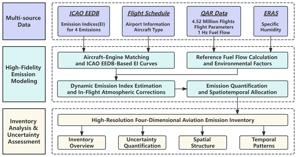
Figure 1 presents the technical framework of this study, comprising three sequential stages. The first stage integrates multi-source data, including 1 Hz QAR records with fuel-flow and flight/ambient parameters from 4.52 million flights in 2023, flight schedule and aircraft information, the ICAO Engine Emissions Databank (EEDB), and ERA5 meteorological data. In the second stage, these datasets are integrated into a high-fidelity emission modeling framework. Aircraft are matched to specific engine types to identify the corresponding EEDB-based emission-index (EI) curves, while QAR-derived fuel-flow measurements are converted to reference fuel flow and combined with environmental factors. Dynamic EIs are then estimated and corrected for in-flight atmospheric conditions using the Boeing Fuel Flow Method 2 (BFFM2), with the corrected EIs combined with instantaneous fuel flow to derive second-level emission rates (DuBois and Paynter, 2006; Yoder, 2007). For particulate matter (PM), the First Order Approximation (FOA) method is further applied to distinguish and quantify its major components. These second-level emissions are subsequently aggregated along flight trajectories in space and time to construct a high-resolution four-dimensional aviation emission inventory. The third stage evaluates the resulting inventory in terms of overall emission characteristics, uncertainty, spatial structure, and temporal patterns.
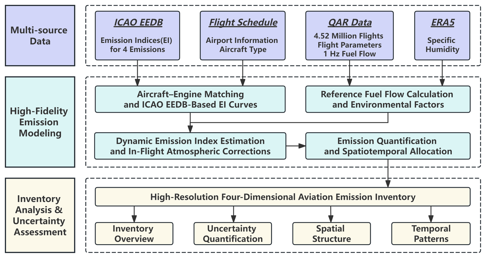
Figure 1Technical framework of this study, including three stages: data integration, core calculation models, and inventory analysis.
2.2 Data Description
2.2.1 QAR Data
The data foundation of this study stems from a massive airborne QAR dataset provided by the Civil Aviation Flight Quality Monitoring Base Station of China. The initial archive contained approximately 4.85 million flight records for the entire year of 2023. As this study aims to construct a civil aviation emission inventory for strictly domestic flights within mainland China, flights with departure or arrival airports outside mainland China, as well as flights involving Hong Kong, Macao, and Taiwan, were excluded. After flight-scope screening and the removal of invalid records, approximately 4.52 million valid domestic flight records were retained, accounting for 93.2 % of the original archive (details of the initial data screening are provided in Table S1 in the Supplement). All retained flights contained complete FF records for the subsequent emission calculations.
The QAR data contains over 2000 parameters throughout the full flight at a frequency of 1 Hz recorded via the airborne Flight Data Acquisition Unit (FDAU) (Dong et al., 2022). Beyond latitude, longitude, and altitude, the QAR data fully covers key thermodynamic parameters such as Fuel Flow (FF), engine rotational speeds (N1/N2), and Exhaust Gas Temperature (EGT). Moreover, it captures real-world environmental parameters, including static air temperature, static pressure, and wind speed (Table 1). Compared to studies relying on generic performance models like BADA, the direct use of airborne measured parameters significantly reduces fuel estimation biases caused by idealized assumptions (Wilkerson et al., 2010; Yanto and Liem, 2018).
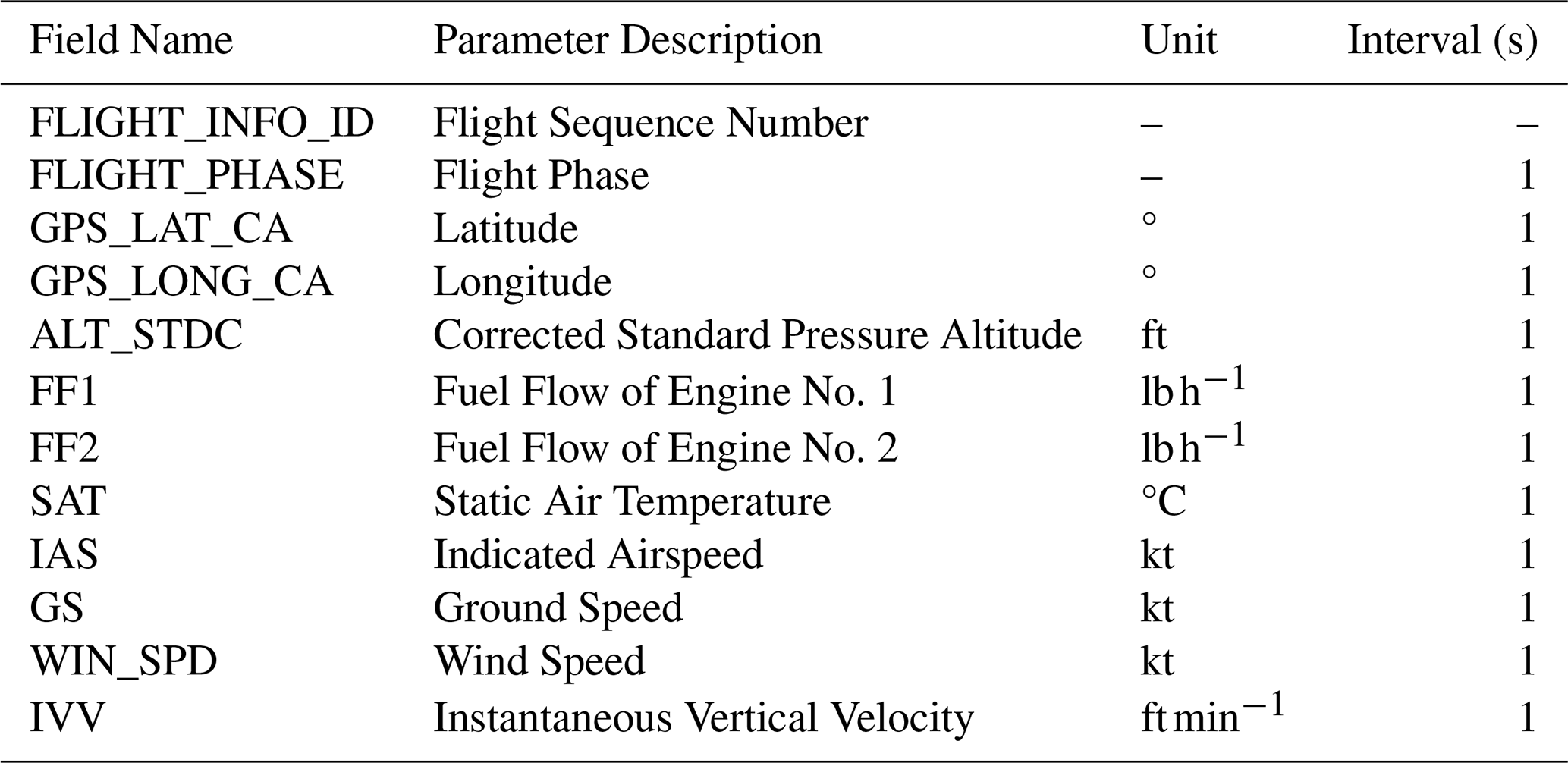
To ensure consistency among the 1 Hz QAR parameters, a common observation index was used as the temporal reference, and all target variables were aligned on this native 1 Hz sequence. Missing observations arising from incomplete QAR records were identified at the observation level, while values violating parameter-specific physical constraints were treated as invalid and converted to missing observations. The screening included negative fuel-flow values, altitudes above 15 000 m, and SAT values outside the physically plausible atmospheric range, together with corresponding constraints for other target variables (Gariel et al., 2011). The observation-level missing rates were then calculated from the combined effects of originally missing and quality-control-screened observations, providing the basis for subsequent missing-data reconstruction.
Following the identification of missing observations, a stepwise reconstruction procedure was applied according to the duration and position of individual gaps. Internal gaps of no more than 30 s, bounded by valid observations on both sides, were recovered using local linear interpolation on the native 1 Hz observation sequence. Remaining gaps, including longer gaps and leading or trailing gaps without valid observations on both sides, were reconstructed using historical similar-flight matching. Historical records from the same route and engine type were preferentially searched, followed by same-route records when no qualified engine-specific match was available; the first-ranked matched flight was then used to reconstruct the missing observations. At the flight level, 68.4 % of the retained flights required no reconstruction, 21.2 % were fully resolved by short-gap interpolation, and 10.4 % additionally required historical-flight matching after the interpolation step. The detailed 1 s observation-level reconstruction proportions for all critical parameters are comprehensively summarized in Table S2.
The effects of the reconstruction procedures were evaluated using point-level mask-based validation. For each variable, known valid 1 s observations were masked according to the observed missing rate while preserving the gap structure of the corresponding missing observations. The masked observations were then reconstructed using the same interpolation and historical-flight matching procedures applied to the operational data. The reconstructed values were compared with the original observations at the masked locations using R2, RMSE, and bias. The reconstructed variables were subsequently propagated through the complete emission calculation framework, and the resulting total emissions were compared with those calculated from the original observations. The validation results and corresponding total emission deviations are presented in Table S3, with the absolute deviations in total emissions remaining below 0.01 % for all evaluated pollutants.
To support subsequent phase-resolved emission calculation, the FLIGHT_PHASE field was mapped to numerical codes following the flight phase classification standard of the China Academy of Civil Aviation Science and Technology (CAST). Because FLIGHT_PHASE labels can be imprecise near phase transitions, we cross-validated the segmentation using auxiliary kinematic parameters, including Ground Speed (GS), Indicated Airspeed (IAS), and Inertial Vertical Velocity (IVV), to correct boundary misclassification. This yielded 12 flight phases representing a nominal flight profile; phase definitions are provided in Table S4, and the corresponding baseline altitude trends are shown in Fig. S1 in the Supplement.
2.2.2 ICAO Emission Factor Database
This study adopted the ICAO Engine Emissions Databank (EEDB v31) (EASA, 2025) as the baseline data source for emission calculations. For each engine model identified in the QAR dataset, we established a dedicated emission index mapping table, directly extracting reference Emission Indices (EIs) for NOx, CO, HC, and nvPM at four standard thrust settings (7 %, 30 %, 85 %, and 100 %). For CO2 and SO2, which are excluded from the EEDB, emissions were calculated based on the carbon and sulfur content of the fuel using the Mass Balance Principle. To overcome the limitation that EEDB data characterize only steady-state LTO emissions under standard atmospheric conditions, we used the extracted reference EIs as anchor points to fit emission characteristic curves. Furthermore, we applied the atmospheric correction of emission indices by integrating second-level measured fuel flow and environmental parameters (temperature, pressure, humidity) provided by QAR. This process successfully transformed static standard emission data into dynamic EIs covering the full-flight phase (including LTO and CCD), achieving high-resolution quantification of instantaneous aircraft emissions under real-world meteorological conditions.
2.2.3 Flight Schedule Data
The flight schedule data were also obtained from the 2023 annual operational archive of the Civil Aviation Flight Quality Monitoring Base Station of China (maintained by the China Academy of Civil Aviation Science and Technology, CAST) and cover scheduled civil aviation flights operated within mainland China, excluding Hong Kong, Macao, and Taiwan, throughout 2023. The dataset provides basic flight information, including airport identifiers, aircraft type, engine type, and departure and arrival times (Table 2).
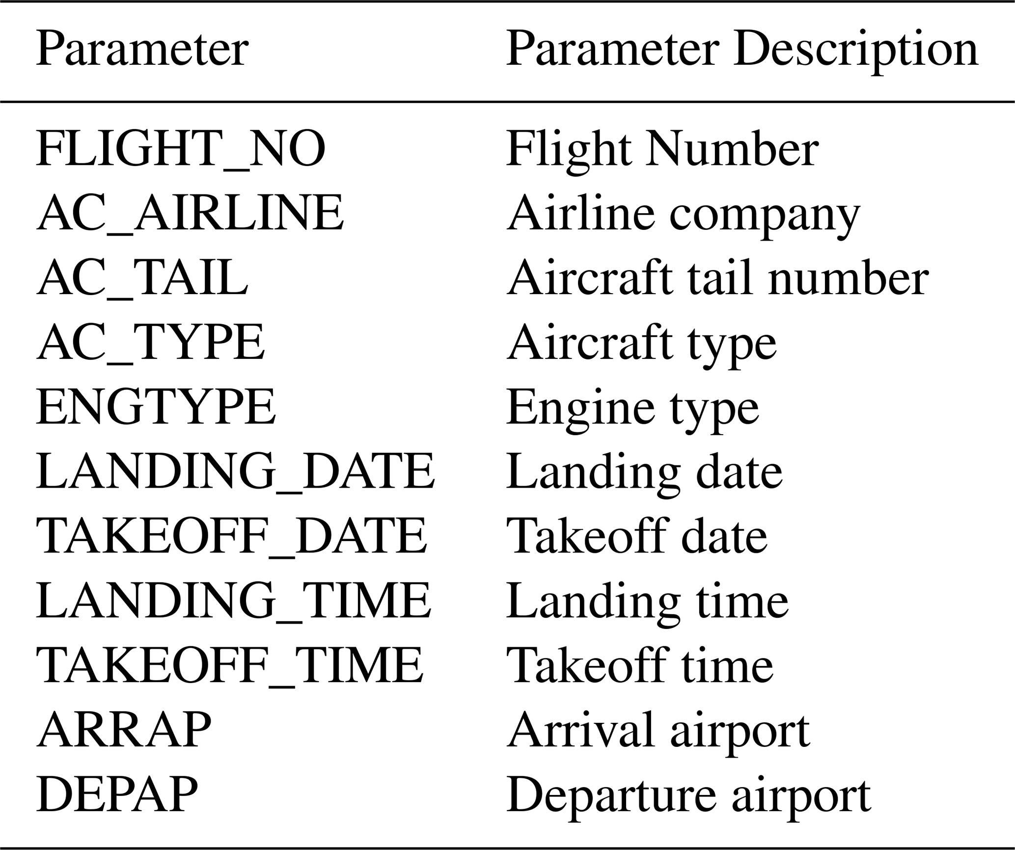
The original time fields were recorded in Coordinated Universal Time (UTC) and were converted to China Standard Time (UTC+8). Because both the QAR data and the flight schedule dataset are exported from the same centralized monitoring platform, the unique flight sequence identifier (FLIGHT_INFO_ID) is natively shared across both original datasets. The processed schedule data were therefore directly linked to the QAR records using FLIGHT_INFO_ID, providing basic flight attributes for the QAR records. The matching of engine types in the schedule data with the International Civil Aviation Organization (ICAO) Engine Emissions Databank (EEDB) is described in Sect. 2.3.1.
2.2.4 Meteorological Reanalysis Data (ERA5)
Aircraft engine NOx emissions are sensitive to ambient atmospheric humidity. In the Boeing Fuel Flow Method 2 (BFFM2) framework, the atmospheric correction of NOx emission indices requires specific humidity in addition to ambient temperature and pressure. Since the QAR data provide in-flight measurements of static pressure and static air temperature but not specific humidity, the ERA5 reanalysis dataset from the European Centre for Medium-Range Weather Forecasts (ECMWF) was incorporated into the emission calculation (Hersbach et al., 2020). For the spatial and temporal domain of this study, ERA5 meteorological data were extracted for the bounding rectangle covering mainland China throughout 2023. Monthly vertical profiles of specific humidity (ω) were obtained for 12 months, with 10 selected pressure levels for each month. The resulting dataset describes the seasonal and vertical variations in atmospheric water vapor over the study region.
The extracted ERA5 specific-humidity data were subsequently matched with the QAR trajectories at the individual observation-point level. For each QAR observation, the flight month was identified from its timestamp, while the QAR-recorded standard pressure altitude was used to determine the corresponding pressure level. The horizontal position of each QAR observation was also associated with the corresponding ERA5 grid location. Based on the month, horizontal grid location, and pressure level, a specific humidity value (ω) was assigned to each QAR observation.
2.3 High-Precision Civil Aviation Emission Model
2.3.1 Engine Matching and EEDB Emission Curve Fitting
Building upon the basic flight attributes linked via the shared FLIGHT_INFO_ID in Sect. 2.2.3, the aircraft registration number (AC_TAIL) and aircraft type (AC_TYPE) were extracted for each flight record and linked to the 2023 Civil Aircraft Static Database maintained by CAST and the Civil Aviation Flight Quality Monitoring Base Station of China (synchronized with official CAAC fleet registration records) to identify the installed engine types. Because engine nomenclature varied across the databases, we developed a seven-level hierarchical matching procedure to link the identified engine types with the International Civil Aviation Organization (ICAO) Aircraft Engine Emissions Databank (EEDB). The procedure was applied sequentially, with the next level activated only when the preceding level failed to return an acceptable match. The corresponding coverage rates for each matching level are summarized in Table S5, while the detailed criteria for the seven-level matching procedure are explicitly documented in the table notes. Among the 4.52 million retained flight records, 98.7 % were assigned two engines, whereas the remaining 1.3 % corresponded to aircraft types inherently equipped with a single engine. More than 82.0 % of the successfully resolved records were obtained through exact or standardized exact matching. A small number of unresolved records were subsequently verified against aircraft registration records and corrected manually. This procedure established an engine-specific reference assignment for the retained QAR records.
Following engine identification, the corresponding reference emission indices (EIs) were extracted from the EEDB and parameterized as continuous functions of per-engine fuel flow. The QAR system records fuel flow independently for each engine at 1 Hz resolution, providing the engine-specific fuel-flow input required for the emission-index parameterization described below. Following a fuel mass-balance formulation, CO2 and SO2 emissions were calculated using fixed EIs rather than thrust-dependent EEDB curves. In accordance with the values adopted in previous aviation emission inventories, fixed EIs of 3150 g kg−1 for CO2 and 1 g kg−1 for SO2 were used (Chen et al., 2021; Howitt et al., 2011). The EEDB reference data were therefore used to parameterize the EIs of NOx, CO, HC, and non-volatile particulate matter (nvPM), whose emission characteristics vary with engine operating conditions.
For the gaseous pollutants, the EEDB provides per-engine reference data at four standardized thrust settings corresponding to 7 %, 30 %, 85 %, and 100 % of maximum rated thrust. These certification points are used as the reference basis for establishing continuous EI–fuel-flow relationships under the fuel-flow-based emission modeling framework (DuBois and Paynter, 2006). Following the established log-log parameterization used in fuel-flow emission models, different fitting strategies were applied according to the observed characteristics of the emission indices. For CO and HC, a bilinear relationship was constructed in log-log space. The first segment was defined by the 7 % and 30 % certification points, while the second segment was represented by a horizontal line at the mean EI level of the 85 % and 100 % points; the two segments were extended to their intersection to form the complete reference curve. For NOx, a point-to-point piecewise linear relationship was established between adjacent certification points in log-log space.
The available EEDB nvPM data were treated separately from the classical BFFM2 gaseous-emission formulation. The EEDB reports engine-specific nvPM mass and number EIs at the same four ICAO certification points for applicable engine types. In this study, the available nvPM reference points were connected using a local point-to-point interpolation scheme in log-log space to provide a continuous empirical EI–fuel-flow relationship over the valid 7 %–100 % reference range. This treatment preserves the local variation represented by the certification data without imposing a single global functional form on the nvPM emission profile. The resulting engine-specific reference EI relationships were subsequently combined with the instantaneous per-engine fuel-flow measurements from QAR to determine the reference EIs corresponding to actual flight operating conditions.
2.3.2 Equivalent Reference Fuel Flow Calculation
To maintain consistency between the QAR observations and the EEDB-based reference curves, the instantaneous fuel flow was first converted to an equivalent reference-condition fuel flow, denoted as Wff, following the fuel-flow normalization procedure of the Boeing Fuel Flow Method 2 (BFFM2).
The ambient static temperature was directly obtained from the Static Air Temperature (SAT) recorded by QAR. For ambient pressure, the QAR-recorded Pressure Altitude was used to derive the corresponding atmospheric pressure based on the standard barometric relationship. Specifically, the ambient pressure (Pamb) was calculated as:
where Pb and Tb are the reference baseline pressure and temperature, L is the temperature lapse rate of the troposphere, h is the pressure altitude recorded by QAR, hb is the baseline height, g0 is the gravitational acceleration, M is the molar mass of Earth's atmosphere, and R is the universal gas constant. The pressure and temperature ratios required by BFFM2 (δamb and θamb) were then calculated by dividing the instantaneous ambient pressure (Pamb) and temperature (Tamb, which is the QAR-recorded SAT) by their respective standard sea-level reference values.
The measured fuel flow for each engine (Wf) was then independently converted to its corresponding reference-condition fuel flow according to the BFFM2 formulation:
where Ma is the instantaneous flight Mach number. This formulation accounts for the effects of ambient pressure, temperature, and flight speed when transforming the fuel flow from flight conditions to the reference condition. The resulting Wff represents the fuel flow corresponding to the observed operating point after normalization to the reference conditions.
2.3.3 Atmospheric Correction of Emission Indices
For each QAR observation, the reference emission indices (EIref) were dynamically determined from the equivalent reference fuel flow (Wff) calculated in Sect. 2.3.2 and the engine-specific emission-index relationships established from the ICAO EEDB in Sect. 2.3.1. The calculated Wff was matched to the corresponding EEDB fuel-flow range, and the fitted relationships were used to determine the reference emission indices of CO, HC, nvPM and NOx at the corresponding operating condition. To avoid extrapolation beyond the empirical EEDB range, Wff values falling outside the available range were constrained to the nearest EEDB boundary before evaluating the corresponding emission-index relationship. The resulting reference emission indices were subsequently corrected for the ambient atmospheric conditions associated with each QAR observation to obtain the flight-condition emission indices (EIflight).
For gaseous pollutants, the Boeing Fuel Flow Method 2 (BFFM2) atmospheric correction was applied. The corrected emission indices of CO and HC were calculated as:
where θamb and δamb are the ambient temperature and pressure ratios defined in Sect. 2.3.2. The NOx emission index was corrected for both temperature and pressure effects and ambient humidity:
where ω is the ambient specific humidity. For particulate matter, the total particulate emission index was resolved into non-volatile particulate matter (nvPM), volatile organic particulate matter, and volatile sulfate particulate matter. The nvPM component was determined from the engine-specific EEDB-based parameterization using the equivalent reference fuel flow (Wff), whereas the volatile components were estimated following the First Order Approximation (FOA) framework (ICAO, 2011). The total particulate emission index was therefore expressed as Eq. (7):
The volatile organic particulate component was estimated from the flight-condition HC emission index using the phase-specific empirical relationship adopted in the FOA methodology:
where EIHC is the HC emission index under actual flight conditions (in g kg−1 fuel) and δm is the phase-specific empirical ratio (in mg g−1). The values of δm are 115, 76, 56.3, and 6.2 for take-off, climb-out, approach, and taxi, respectively. These phase-specific ratios relate the volatile organic particulate emission index to the HC emission index for the corresponding operating mode.
The volatile sulfate particulate emission index was estimated from the fuel sulfur content and the sulfur conversion fraction following the FOA-based formulation:
where FSC is the fuel sulfur content, prescribed as 500 ppm by mass, and ε is the fraction of fuel sulfur converted from S(IV) to S(VI), which was set to 0.024 following the value adopted in the FOA methodology. and MWS are the molecular weights of sulfate and sulfur, respectively, with values of 96 and 32.
For nvPM, the dynamically determined reference emission index (EInvPM,ref) was obtained from the engine-specific EEDB-based parameterization using the equivalent reference fuel flow calculated for each QAR observation. The reference nvPM emission index was then corrected to flight conditions using the Aircraft nvPM Mission Emissions Estimation Methodology, Version 2 (MEEM2) of Ahrens et al. (2025):
where EInvPM,ref is the engine-specific reference nvPM emission index and δamb and θamb are the ambient pressure and temperature ratios, respectively. The MEEM2 correction accounts for the effects of ambient conditions on nvPM emissions through fuel-flow- and altitude-dependent relationships consistent with the BFFM2-based treatment of flight conditions.
2.3.4 Emission Calculation and 4D Grid Aggregation
Following the atmospheric correction of emission indices, pollutant emissions were quantified at the individual-engine level using the 1 Hz QAR observations. The instantaneous emission mass for a given pollutant x during each sampling interval (Δt=1 s) is inherently the product of the recorded fuel flow rate and the corresponding flight-condition emission index. Accordingly, the total emission mass (Mx) generated by an individual flight was obtained by integrating these second-by-second emissions across all operating engines and the complete flight period:
where Neng is the number of operating engines, T is the total number of 1 Hz observations, FFi,t is the actual fuel flow rate of engine i at time t, and is the flight-condition emission index. This engine-level temporal integration allows the emission contribution of each engine to be quantified independently according to its transient operating conditions.
The second-by-second emission records were subsequently aggregated into a four-dimensional spatiotemporal emission grid. The horizontal domain was discretized at a resolution of 0.1°×0.1°, while the vertical dimension was divided into 1000 m altitude layers. The temporal dimension was aggregated by calendar month. For each 1 Hz QAR observation, the calculated emission mass was assigned to the corresponding horizontal grid cell, altitude layer, and calendar month based on the actual aircraft longitude, latitude, and pressure altitude. Emissions from all trajectory observations falling within the same spatiotemporal grid cell were then summed.
The resulting dataset contains monthly four-dimensional emission fields for CO2, SO2, NOx, PM, CO, and HC. This bottom-up aggregation retains the spatial and temporal distribution of individual flight trajectories while converting the high-frequency emission estimates into a standardized 4D emission inventory.
2.4 Uncertainty Propagation
To characterize the propagation of prescribed input uncertainties through the aircraft emission calculation chain described in Sect. 2.3, Monte Carlo simulations were conducted for the QAR-, ADS-B-, and SFD-based inventory frameworks. The prescribed uncertainties were grouped into four major sources: fuel-flow uncertainty (FF), environmental uncertainty (Env), emission-index uncertainty (EI), and operational uncertainty (Ops). For strictly positive multiplicative variables, such as fuel-flow bias, distance and time factors, and emission indices, mean-normalized log-normal distributions were used to avoid non-physical negative values. Ambient temperature was perturbed using an additive Gaussian distribution. For fuel-flow uncertainty, the bias was combined with temporally correlated multiplicative and additive perturbations. The temporal correlation of these perturbations was represented using first-order autoregressive AR(1) processes, allowing the simulated fuel-flow uncertainty to vary along the flight profile while retaining temporal dependence between consecutive observations. The corresponding uncertainty parameters for the QAR-, ADS-B-, and SFD-based frameworks are summarized in Table 3.
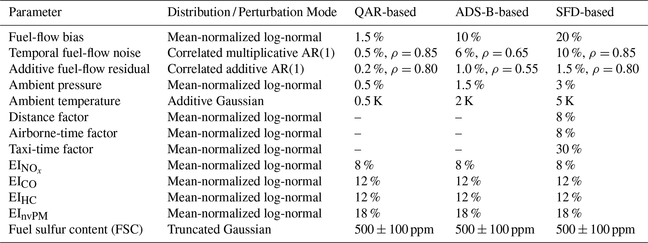
The fuel-flow uncertainties were parameterized according to the measurement or reconstruction procedures used in each framework. For the QAR-based approach, a 1.5 % systematic bias was assigned, slightly exceeding the typical fuel-flow sensor accuracy of ±1 % (Baumann et al., 2021). The temporally correlated component was set to 0.5 %, consistent with the 0.2 %–0.5 % average dynamic errors reported in the same study. An additional 0.2 % additive residual was prescribed to account for unresolved measurement variability. For the ADS-B-based approach, fuel flow is reconstructed from trajectory-derived aircraft states and performance models. Krajček Nikolić et al. (2024) reported phase-dependent errors reaching 17.2 % during initial climb and −53.5 % during approach, although the mean whole-flight error was 1.2 % (standard deviation: 1.3 %) based on five flights. Considering these phase-dependent discrepancies, a 10 % systematic bias was adopted as a conservative modelling allowance. The 6 % temporal component and 1.0 % additive residual were prescribed to represent time-varying reconstruction errors and unresolved local discrepancies. For the SFD-based approach, a 20 % systematic bias was adopted, informed by the approximately 17.7 % standard deviation of flight-level fuel-burn errors reported for schedule-derived trajectories by Lee (2005). The 10 % temporal component and 1.5 % additive residual were prescribed to represent additional uncertainties in the generalized fuel-flow profile.
Environmental uncertainties were specified according to the data sources used in each framework. For QAR, pressure and temperature perturbations were set to 0.5 % and 0.5 K, respectively, representing small allowances for onboard measurement uncertainty. For ADS-B, which uses ERA5 meteorological fields, these values were increased to 1.5 % and 2 K. The 2 K temperature perturbation provides a conservative allowance relative to the approximately 0.57–1.66 K upper-air temperature observation errors reported for ERA5 (Hersbach et al., 2020), while the pressure perturbation was prescribed to account for residual meteorological uncertainty. For SFD, pressure and temperature perturbations were further increased to 3 % and 5 K, respectively, to reflect the absence of flight-specific meteorological information (ICAO, 1993). Distance and airborne time were assigned 8 % perturbations to represent differences between scheduled and actual operations, while taxi time was assigned a larger 30 % perturbation to account for operational variability (Simaiakis and Balakrishnan, 2016; Teoh et al., 2024).
Uncertainties in the emission indices of NOx, CO, HC, and nvPM were set to 8 %, 12 %, 12 %, and 18 %, respectively, and applied consistently across the three frameworks. These values represent prescribed residual uncertainties in engine-specific emission parameters and their application to in-service conditions (Kim et al., 2007; Wasiuk et al., 2015). Koopmann et al. (2014) reported approximately ±10 % uncertainty for BFFM2 calculations under non-reference conditions, as well as engine-to-engine variability of ±16 %, ±23 %, and ±54 % for NOx, CO, and HC, respectively. The adopted values therefore represent residual perturbations after engine-type matching, rather than the full range of engine-to-engine variability. The 18 % nvPM perturbation was prescribed to account for uncertainties in particulate emission parameters. Fuel sulfur content was sampled from a truncated Gaussian distribution to represent its variability and influence on SO2 and sulfate emissions (Kapadia et al., 2016). The resulting input uncertainties were propagated through 10 000 Monte Carlo simulations, and output uncertainty was quantified using the coefficient of variation (CV), defined as the ratio of the standard deviation to the mean of the simulated emissions.
To quantify the relative contribution of different uncertainty sources without assigning residual variance subjectively, a Shapley-based variance decomposition was further applied. Four uncertainty sources (FF, Env, EI, and Ops) were considered as players in the variance attribution. For each framework, all 24=16 possible combinations of these uncertainty sources were evaluated using independent Monte Carlo simulations. Let V(S) denote the variance of the simulated emission estimates when the subset S of uncertainty sources is activated. The Shapley contribution of source k was calculated as:
where N denotes the complete set of uncertainty sources and n=4. This formulation accounts for the marginal contribution of each uncertainty source across all possible source combinations and therefore incorporates the effects of interactions among uncertainty sources. The resulting contributions were normalized by the total output variance to obtain the relative variance contribution of each source.
3.1 Overview of the 2023 China Aviation Emission Inventory
Derived from 1 Hz operational observations across approximately 4.52 million QAR-recorded flights, this study compiled a four-dimensional emission inventory for purely domestic civil aviation flights within mainland China in 2023, excluding flights involving Hong Kong, Macao, and Taiwan as well as international inbound and outbound operations. Under this system boundary, total annual fuel consumption is estimated at 23.7 Mt, corresponding to total emissions of 74.6 Mt for CO2, 311.84 kt for NOx (reported as NO2 mass equivalent), 73.5 kt for CO, 6.02 kt for HC, 23.69 kt for SO2, and 2.00 kt for PM. To evaluate the macroscopic consistency of the inventory, the QAR-based fuel consumption was compared against official industry statistics released by the Civil Aviation Administration of China (CAAC, 2024). Based on the annual transport turnover and average fuel efficiency reported by the CAAC, national domestic fuel consumption in 2023 is estimated at approximately 25.03 Mt, yielding a relative difference of 5.3 % compared with our bottom-up summation. Here, the CAAC statistical value serves as an independent national-scale benchmark of overall magnitude. While the retained QAR archive captures approximately 96.8 % of the commercial flight movements reported by the CAAC, flight-count coverage does not correspond directly to fuel-burn coverage because individual flights vary in aircraft type, stage length, and payload. Overall, the 5.3 % difference indicates good agreement in magnitude between the integration of 1 Hz onboard fuel-flow measurements and top-down statistical accounting. The statistical distribution of major engine models and departure airports comprising this domestic fleet is detailed in Fig. S2. Furthermore, monthly variations in flight activity and emission totals across the six species are presented in Fig. S3.
Compared with previous aviation inventories, the estimates in this study demonstrate strong macroscopic alignment in species directly proportional to fuel burn. Our total fuel consumption of 23.7 Mt and the corresponding CO2 emissions of 74.6 Mt are broadly consistent with top-down statistical baselines and recent discrete-flight assessments for the national fleet. In that CO2 generation is strictly governed by stoichiometric fuel mass balance, this baseline agreement validates the comprehensive capture of flight activities and the overall representation of route network intensity.
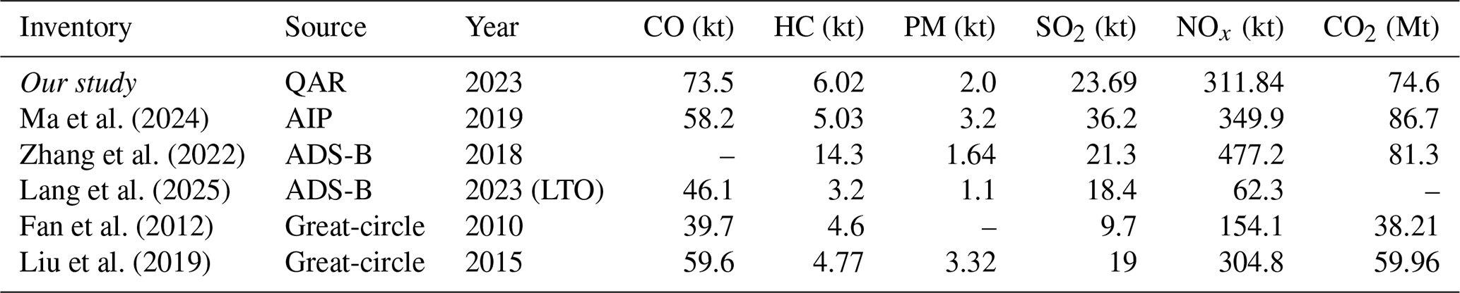
Building upon this validated baseline, meaningful divergences emerge in thermodynamically sensitive pollutants and incomplete combustion products (Table 4). Specifically, the estimated CO emissions (73.5 kt) are higher than previous full-flight values (39.7–59.6 kt), whereas NOx emissions (311.84 kt) are substantially lower than trajectory-modeled upper estimates (up to 477.2 kt). Rather than mere methodological noise, these discrepancies highlight the inherent limitations of relying on idealized operating profiles. Schedule- and trajectory-based models often underrepresent prolonged low-power ground operations, such as extended taxiing and holding which disproportionately elevate CO generation due to incomplete combustion. Conversely, generic performance models frequently assume maximum rated thrust during takeoff and climb, leading to a systematic overestimation of peak combustor temperatures and thermal NOx formation (Koudis et al., 2017). By coupling 1 Hz measured fuel flow with actual in-flight ambient temperature, pressure, and specific humidity, our QAR-based framework directly captures real-world transient operations (e.g., reduced-thrust takeoffs) and dynamic environmental effects. This approach transitions the emission estimates from model-parameterized approximations to a physically constrained operational baseline, with the corresponding uncertainty propagation formally evaluated in Sect. 3.2.
Table 4Comparison of estimated annual civil aviation emissions in China across different inventory studies.
3.2 Uncertainty Propagation and Contributions of Uncertainty Sources
Figure 2 presents the Monte Carlo distributions obtained by propagating the prescribed uncertainty distributions through the three parallel inventory frameworks. For CO2, the resulting CVs strictly scale with the fidelity of the activity data, yielding 1.5 %, 10.2 %, and 23.2 % for the QAR-, ADS-B-, and SFD-based frameworks, respectively. Because CO2 generation is directly governed by a stoichiometric mass balance, its variance serves as a baseline indicator of macroscopic fuel-flow uncertainty, isolated from complex combustion physics. The horizontal comparison across the three frameworks clearly demonstrates the value of physical observations: compared to the SFD framework, which relies heavily on generic assumptions, the high-frequency measurements in the QAR framework effectively constrain the fundamental activity and fuel-flow uncertainties.
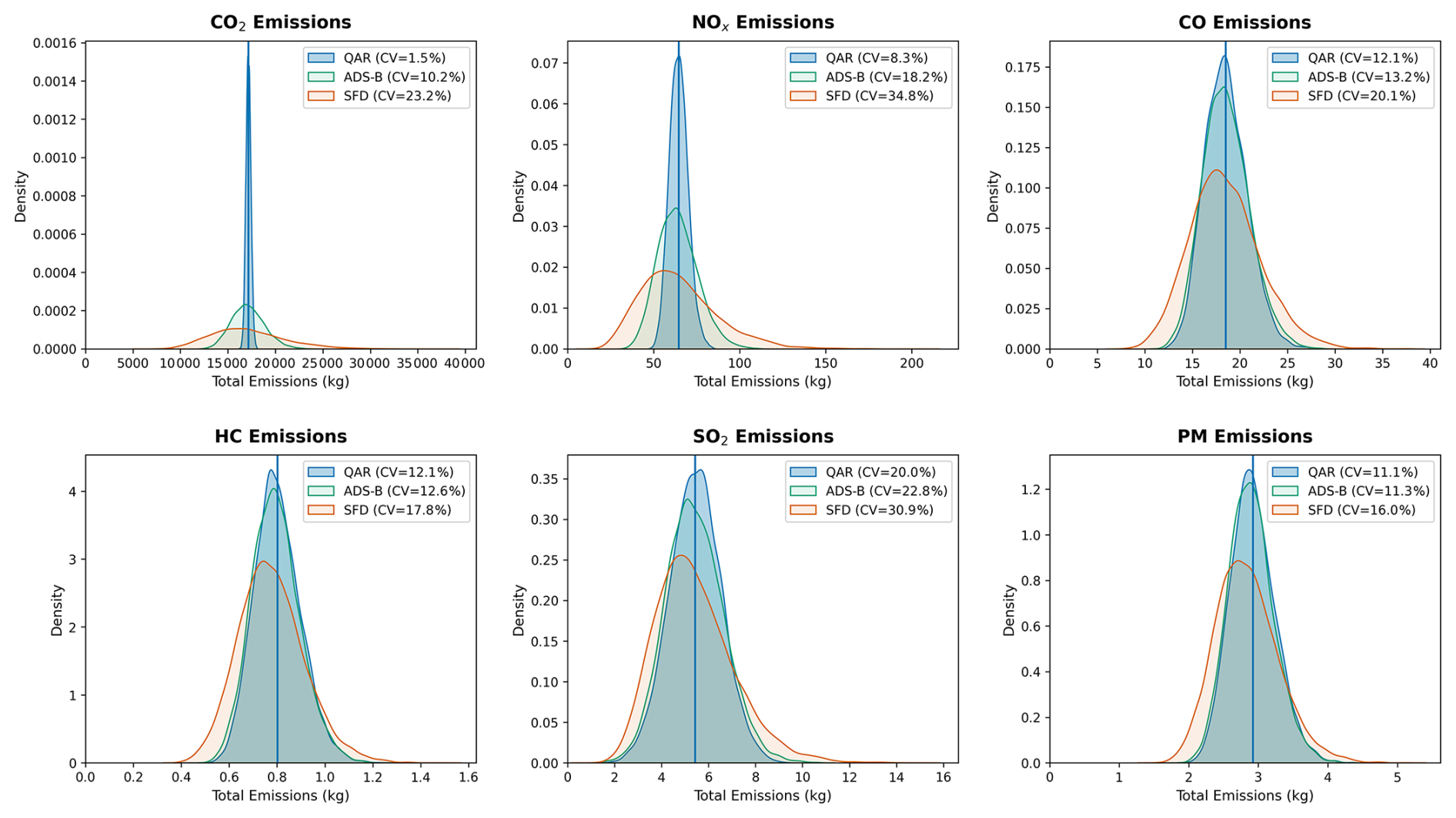
Figure 2Monte Carlo uncertainty distributions of the estimated totals for six pollutants across the different inventory compilation frameworks.
This error-constraining capability is particularly critical for thermodynamically sensitive pollutants. For NOx, the CVs increase substantially to 8.3 %, 18.2 %, and 34.8 % for the QAR, ADS-B, and SFD frameworks, respectively. Unlike CO2, NOx formation is highly non-linear and extremely sensitive to peak combustor temperature and ambient humidity. In the SFD and ADS-B frameworks, errors in reconstructed thrust profiles compound with biases in coarse meteorological reanalysis data during the atmospheric correction process. Conversely, the QAR framework couples instantaneous fuel flow with concurrent onboard pressure and temperature observations (Olsen et al., 2013), largely eliminating this compounded meteorological and operational variance and tightly bounding the NOx estimates.
However, this substantial reduction in variance does not apply equally to all species. For incomplete-combustion products (CO, HC) and non-volatile particulate matter (PM), the uncertainty distributions plateau. The CVs for CO, HC, and PM decrease from the SFD framework (20.1 %, 17.8 %, and 16.0 %) to the ADS-B framework (13.2 %, 12.6 %, and 11.3 %), but improve only marginally under the QAR framework (12.1 %, 12.1 %, and 11.1 %). Similarly, the SO2 CV drops from 30.9 % to 20.0 %, ultimately bounded by the prescribed fuel sulfur content variation. This horizontal plateau indicates that for pollutants governed by complex localized combustion inefficiencies and soot nucleation, resolving trajectory and fuel-flow errors is insufficient to eliminate overall inventory uncertainty.
The Shapley-based variance decomposition (Fig. 3) provides the mathematical mechanism underlying this plateau, using CO as a representative case. In the SFD framework, uncertainty is distributed across multiple confounding sources, with emission-index (EI) parameterization, fuel-flow/environmental, and operational uncertainties accounting for 36.4 %, 35.0 %, and 28.7 % of the variance, respectively. Consistent with the limitations of generic performance modeling, the larger prescribed uncertainties in reconstructed fuel-flow and operational variables make these kinematic sources increasingly important, resulting in a highly distributed uncertainty structure (Akçelik and Besley, 2003). However, once actual flight trajectories and onboard thermodynamic states are constrained by QAR observations, the combined variance contribution of these activity and environmental sources collapses to 1.4 %. Consequently, the inherent uncertainty within the EEDB-based EI parameterization emerges as the dominant constraint, accounting for 98.6 % of the residual variance in the QAR framework. This source-level attribution demonstrates a fundamental shift in the rate-limiting step of inventory precision: while high-fidelity onboard measurements successfully resolve kinematic and environmental errors, further accuracy improvements for non-linear pollutants are now strictly bottlenecked by the empirical emission-index models.
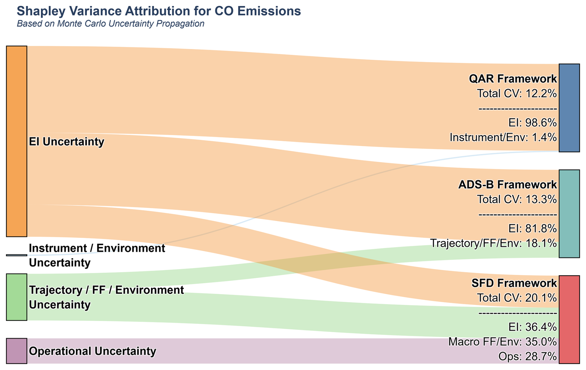
Figure 3Shapley-based variance decomposition of CO emissions across the QAR, ADS-B, and SFD inventory frameworks. The flow widths indicate the relative contribution of each corresponding uncertainty source to the total propagated variance.
3.3 Temporal Evolution Characteristics
Figure 4 shows the relative contribution of each flight phase to total emissions in the 2023 QAR dataset. The Cruise phase dominates cumulative emissions for most pollutants, reflecting its share of total flight duration: it accounts for 43.3 % of total fuel consumption (and, correspondingly, CO2 and SO2), 27.7 % of HC, 34.5 % of CO, 36.1 % of NOx, and 42.8 % of PM.
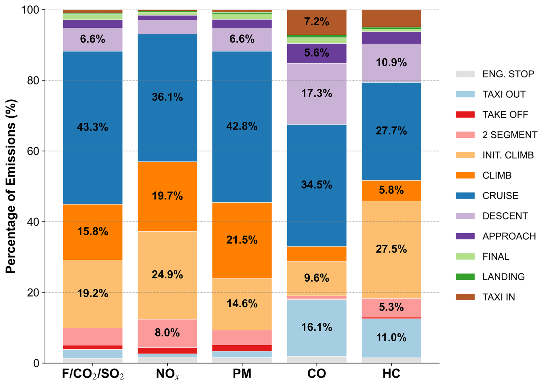
Figure 4Distribution proportions of fuel consumption and pollutant emissions across twelve refined flight phases.
This duration-driven dominance does not hold for pollutants governed by combustion efficiency rather than fuel throughput. HC and CO formation increases as combustion efficiency falls (Liu et al., 2019), so both are concentrated during low-power ground operations: taxiing contributes 21.9 % of total HC (11.0 % Taxi Out, 10.9 % Taxi In) and 23.3 % of total CO (16.1 % Taxi Out, 7.2 % Taxi In) with CO showing a larger Taxi-Out contribution than Taxi-In, while HC exhibits nearly equal contributions from Taxi-Out and Taxi-In. Under idle thrust, lower combustor temperature and pressure impair fuel atomization and mixing, sharply raising HC and CO generation rates (Lee et al., 2010; Ma et al., 2025).
PM exhibits a strong dependence on high-thrust flight operations, with Cruise, Climb, and Initial Climb accounting for 42.8 %, 21.5 %, and 14.6 % of total PM emissions, respectively, consistent with the soot formation mechanism described by Lobo et al. (2020), in which high-temperature and high-pressure combustion during high-thrust operations promotes soot nucleation and growth. Taken together, these phase-resolved contributions show that the dominant emission phases differ across pollutants: fuel-scaling species (CO2 and SO2) are strongly associated with fuel-consuming flight duration, CO and HC show substantial contributions from low-power ground and approach-related operations, whereas PM is more strongly associated with high-thrust flight phases. This distinction is only resolvable through phase-level QAR segmentation and provides important insights into the spatial and operational distribution of aviation emissions, particularly for near-airport operations.
To examine the temporal variations in aircraft emissions under changing flight conditions, a representative B737-800 flight was selected to construct a second-by-second emission profile (Fig. 5). The six pollutants exhibit distinct temporal patterns across the different flight phases, with more pronounced fluctuations during takeoff, descent, approach, and taxiing.
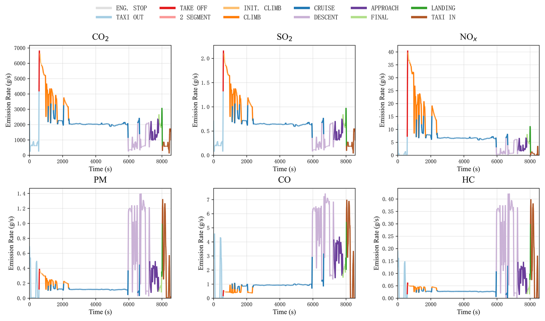
During takeoff and climb, CO2 and SO2 closely follow the fuel-flow profile, with elevated emission rates during high-power operation. NOx also increases substantially during these phases, reflecting its sensitivity to combustion conditions. CO, HC, and PM show more pronounced short-term fluctuations, indicating their stronger response to changes in engine operating conditions. The variations during climb also show repeated short-term changes rather than a smooth monotonic trend.
During cruise, the emission rates of CO2 and SO2 become relatively stable, while NOx also remains comparatively steady. CO and HC decrease substantially compared with the takeoff and low-power phases but remain at low non-zero levels throughout cruise. This reflects the continuous fuel consumption and the non-zero emission indices obtained from the EEDB-based parameterization. The PM emission rate likewise remains relatively low and stable during most of the cruise phase.
A clear transition occurs during descent and approach. As engine power decreases, CO and HC emission rates increase and exhibit frequent short-duration fluctuations. PM shows a similar increase in variability, inherently linked to the HC-dependent volatile organic particulate component described in Sect. 2.3.3. These features indicate that low-power operating conditions produce substantially more variable emissions of incomplete-combustion products and particulate matter than the relatively stable cruise condition.
During landing and taxi-in, CO, HC, and PM continue to exhibit pronounced transient variations, while CO2 and SO2 remain strictly coupled with changes in fuel flow. Concurrently, thrust reverser deployment at landing produces a distinct transient emission spike, corresponding directly to the rapid thrust transition and associated combustion dynamics (Schürmann et al., 2007). Overall, the full-flight profile demonstrates that second-by-second QAR observations successfully resolve short-duration emission peaks during phase transitions and low-power operations. These acute, high-intensity emission events, which are largely smoothed out in temporally aggregated average-factor models, are critical components for accurately characterizing near-airport air quality and human exposure (Woody et al., 2011).
3.4 Spatial Dimension Analysis
3.4.1 Reconstruction of 3D Flight Trajectories and Emission Characteristics for Typical Routes
Using high-frequency QAR data with 0.001° longitude/latitude precision, ∼0.03 m (0.1 ft) altitude precision, and 1 s temporal resolution, we reconstructed three-dimensional flight trajectories and vertical profiles for all flights between Beijing Capital International Airport (ZBAA) and Chengdu Tianfu International Airport (ZUTF) in March 2023. This route was selected as a representative case for detailed trajectory-level analysis: it is one of the trunk corridors identified in the network-level analysis above, its ∼1600 km stage length is long enough to capture a full climb–cruise–descent profile without truncation by short-haul operating constraints, and both endpoints are high-frequency hub airports, providing a large and consistent sample within a single month.
The observed three-dimensional tracks depart substantially from the ideal great-circle route, forming multi-segment polylines (Fig. 6a). Divergence and distortion are concentrated in the terminal areas around both airports, where trajectory bundles spread across a wider range of headings during low-altitude approach and departure, which is consistent with sequencing and holding operations under air traffic control guidance (del Pozo Domínguez et al., 2023). Figure 6b shows a corresponding fine structure in the vertical dimension: outbound and inbound cruise altitudes are strictly stratified, consistent with the odd/even altitude allocation under RVSM rules (ICAO, 2001).
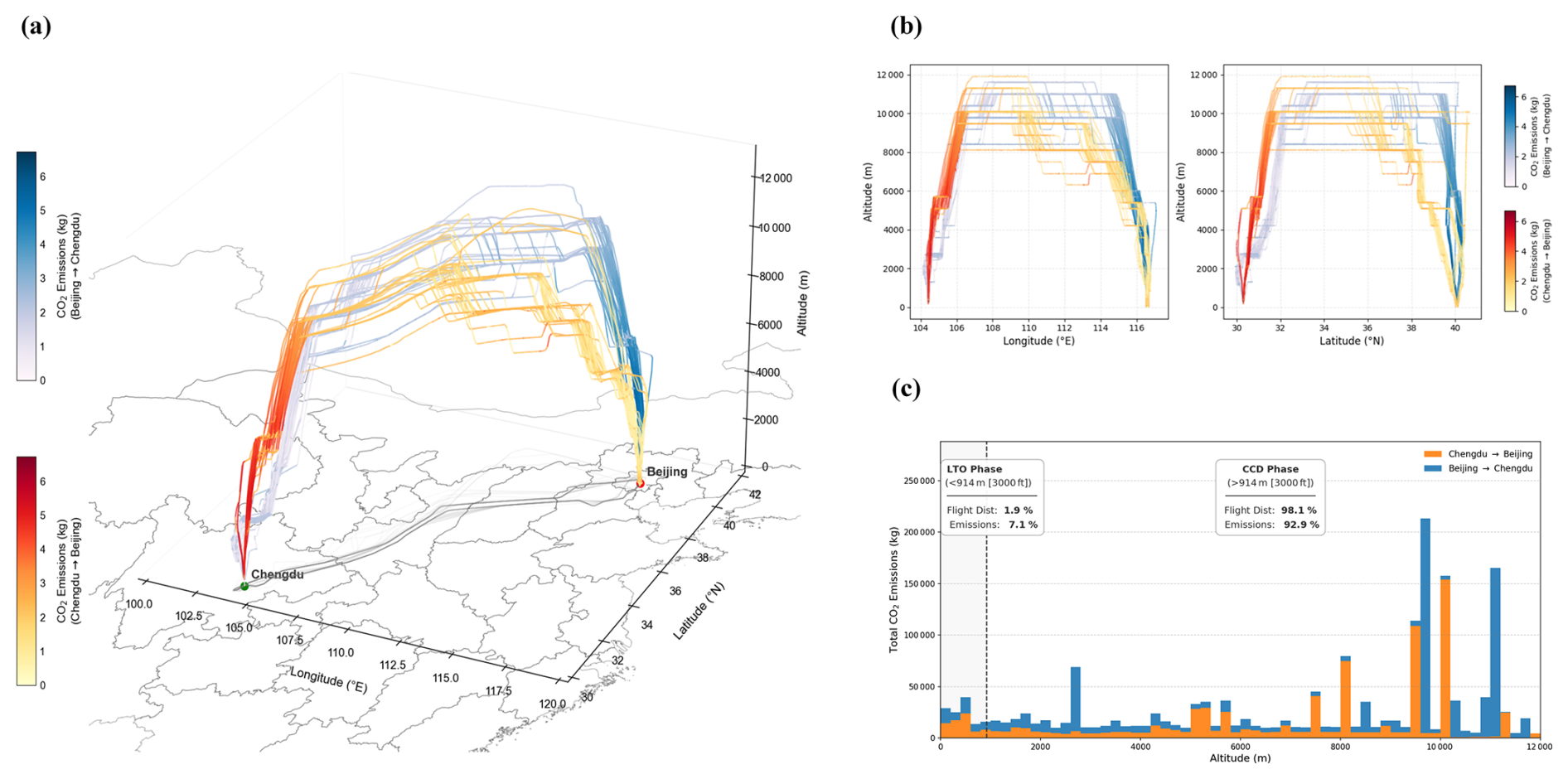
Figure 6(a) Three-dimensional visualization of real-world flight trajectories between Beijing (ZBAA) and Chengdu (ZUTF), colored by instantaneous CO2 emission rates. (b) Orthogonal projections of flight trajectories for the ZBAA–ZUTF route onto longitude-altitude and latitude-altitude planes, where blue and orange-red spectra denote outbound (to Chengdu) and inbound (to Beijing) flights, respectively. (c) Vertical profile of total accumulated CO2 emissions for the ZBAA–ZUTF route, aggregated in 200 m altitude bins.
The vertical distribution of CO2 emissions along the Chengdu–Beijing and Beijing–Chengdu routes exhibits pronounced phase-specific characteristics (Fig. 6c). Using 3000 ft (approximately 914 m) as the boundary between the LTO and CCD phases, the LTO phase accounts for only 1.9 % of the total flight distance but contributes 7.1 % of total CO2 emissions. In contrast, the CCD phase above 914 m accounts for 98.1 % of the flight distance and 92.9 % of total CO2 emissions. The disproportionately higher emission share of the LTO phase relative to its distance share reflects the elevated fuel burn rates per unit distance associated with takeoff, initial climb, approach, taxi, and other low-altitude operations. The vertical distribution also exhibits pronounced emission peaks at several cruise altitudes, particularly around 9600–10 000 m, reflecting the concentration of flight operations within assigned cruise flight levels. Here, the resolved CO2 profile serves as a direct indicator of fuel-burn intensity and vertical operational clustering. Because the intense low-altitude fuel burn during the LTO phase occurs near airports and populated terminal areas, the co-emitted criteria pollutants (specifically NOx and PM) within this layer are of particular relevance as inputs for subsequent dispersion modeling and local air-quality assessments (Unal et al., 2005; Wang et al., 2023).
3.4.2 Analysis of High-Resolution Spatial Pattern of Aviation Carbon Emissions in China
The spatial distribution of aviation carbon emissions closely tracks China's economic geography, characterized by a pronounced east-west gradient (Fig. 7a). The Beijing-Tianjin-Hebei, Yangtze River Delta, and Pearl River Delta agglomerations are linked by a dense route network that produces continuous high-flux coverage across the eastern coastal and central regions. The western region, by contrast, shows a sparser, radial pattern centered on regional hubs such as Urumqi and Kunming, consistent with the concentration of air transport demand in areas of higher economic activity and population density.
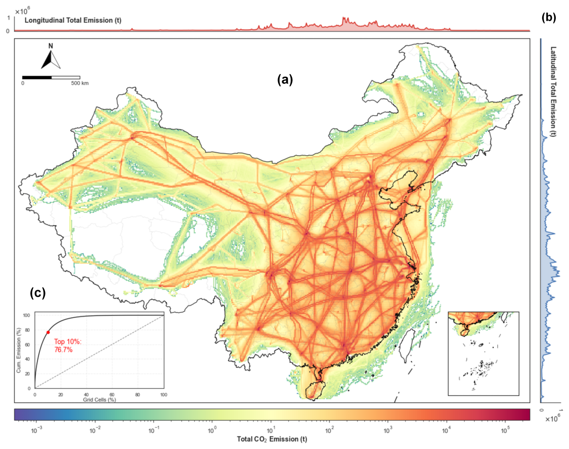
Figure 7(a) Spatial intensity map illustrating the geographical distribution of emission loads. (b) Latitudinal and longitudinal marginal cumulative profiles, depicting the directional accumulation of emissions. (c) The Lorenz curve quantifies the spatial inequality and concentration of emissions.
At finer spatial resolution, this pattern resolves into a hub-and-corridor structure. Continuous high-value pixels trace national trunk routes such as Beijing-Shanghai, Beijing-Guangzhou, and Shanghai-Chengdu, corresponding to the steady fuel consumption of the cruise (CCD) phase at high altitude. The localized emission hotspots at route endpoints instead reflect the accumulation of high-thrust, high-frequency LTO operations in near-ground airspace. Cruise emissions therefore appear as continuous linear flux along corridors, while LTO emissions appear as point-like concentrations at airports.
Figure 7b quantifies this east-west inequality: the meridional cumulative curve rises sharply east of 100° E, and the zonal curve peaks near 30° N, consistent with the role of the Yangtze River Economic Belt as the primary corridor linking eastern, central, and western air traffic. Figure 7c shows that emissions are highly concentrated at the grid level, with the top 10 % of grid cells accounting for 76.7 % of total CO2 emissions. This concentration indicates that a small number of trunk corridors and hub airports account for a disproportionate share of aviation's carbon footprint, which is relevant to where operational or routing interventions would have the greatest effect on total emissions.
To assess whether the hub-and-corridor pattern identified above is statistically significant, we conducted a spatial autocorrelation analysis on 0.1°×0.1° gridded emissions. Figure 8a shows pronounced spatial clustering: High-High units align closely with trunk routes such as Beijing–Shanghai, Beijing-Guangzhou, and Shanghai-Chengdu, connecting the hub cities of Beijing, Shanghai, Guangzhou, and Chengdu, while Low-Low units cover most of the non-route areas in the northwest and interior. Emissions are therefore not spatially diffuse but organized along the route network itself.
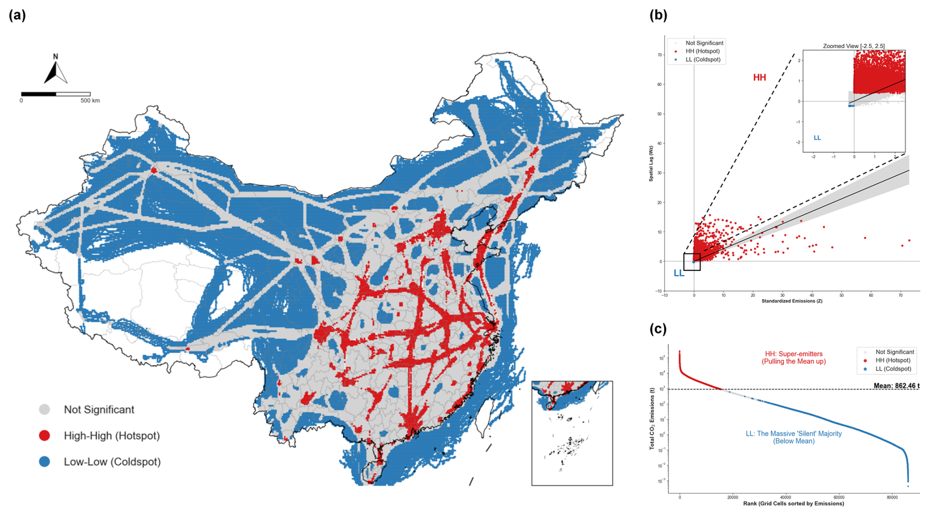
Figure 8(a) LISA (Local Indicators of Spatial Association) cluster map showing local spatial agglomeration types. (b) Moran's scatter plot illustrating global spatial auto correlation. (c) Rank-size distribution plot revealing the heavy-tailed characteristic of emission intensity across grid cells.
This clustering is confirmed by the global Moran's I (0.4227, p<0.05) and by the quadrant distribution in Fig. 8b, where samples concentrate almost entirely in the High-High and Low-Low quadrants, with very few falling in the High-Low or Low-High transition quadrants. The scarcity of transition cases is consistent with the physical constraint that air traffic is confined to narrow, fixed-width corridors: emissions drop sharply outside a route's footprint rather than tapering gradually, leaving little room for intermediate grid values.
Figure 8c shows that grid-level emissions follow a power-law distribution, with a small number of high-load grid cells accounting for a disproportionate share of the cumulative total. Combined with the LISA results, this indicates that China's aviation emissions are concentrated both structurally, along a limited set of corridors and hubs and statistically, in a small subset of grid cells that dominate the national total.
The high-resolution 4D gridded aviation emission inventory dataset generated in this study is freely available at Zenodo via https://doi.org/10.5281/zenodo.23334964 (Lu et al., 2026). The dataset is provided in NetCDF format with a horizontal spatial resolution of 0.1°×0.1° and a vertical resolution of 1000 m, including emission fields for CO2, NOx, SO2, PM, CO, and HC.
This study developed a four-dimensional aviation emission inventory for China's domestic civil aviation sector in 2023, built from onboard Quick Access Recorder (QAR) measurements across approximately 4.52 million flights (representing ∼96.8 % of commercial flight movements reported by the CAAC). Incorporating 1 Hz per-engine fuel flow with observed flight trajectories, onboard ambient temperature and pressure measurements, and ERA5 specific humidity profiles, the inventory characterizes aviation emissions under actual operating conditions rather than relying solely on schedule-based or performance-model proxies.
For 2023, total fuel consumption from purely domestic flights within mainland China is estimated at 23.7 Mt, corresponding to 74.6 Mt CO2, 311.84 kt NOx, 73.5 kt CO, 6.02 kt HC, 23.69 kt SO2, and 2.00 kt PM. While fuel consumption, CO2, and SO2 show good consistency with official CAAC statistics and previous inventories, larger differences are observed for CO, HC, NOx, and PM. These differences reflect the high sensitivity of non-linear combustion species to engine matching, reference fuel-flow conversion, EEDB curve parameterization, and in-flight atmospheric corrections.
The Monte Carlo uncertainty propagation and Shapley variance decomposition clarify how input uncertainties behave across different inventory frameworks. Replacing schedule-based (SFD) and performance-modeled (ADS-B) fuel-flow estimates with onboard QAR measurements substantially reduces the output uncertainty for fuel- and environment-sensitive species, narrowing the coefficient of variation (CV) from 23.2 % (SFD) and 10.2 % (ADS-B) to 1.5 % (QAR) for CO2, and from 34.8 % (SFD) and 18.2 % (ADS-B) to 8.3 % (QAR) for NOx. However, for incomplete-combustion products, particulate matter, and sulfur species, the CVs under the QAR framework – 12.1 % for CO, 12.1 % for HC, 11.1 % for PM, and 20.0 % for SO2 – are only modestly lower than those under the ADS-B framework (13.2 %, 12.6 %, 11.3 %, and 22.8 %, respectively). As demonstrated by the Shapley attribution, once flight trajectories and fuel flow are constrained by observations, the remaining uncertainty is dominated by the prescribed uncertainties in the EEDB emission-index parameterizations (contributing 98.6 % of the variance for CO in the QAR framework) and fuel sulfur content. This indicates that while QAR observations effectively eliminate activity- and fuel-model uncertainties, further reductions in total emission uncertainty depend primarily on refining engine emission-index models rather than activity inputs alone.
At the process level, the 1 Hz phase-resolved analysis highlights distinct emission regimes across flight phases. Cruise operations dominate cumulative fuel consumption (43.3 %), (43.3 %), PM (42.8 %), and NOx (36.1 %), whereas incomplete-combustion products show substantial contributions from low-power ground operations, with taxiing accounting for 23.3 % of total CO and 21.9 % of total HC emissions. Second-by-second flight profiles further capture transient emission fluctuations during climb thrust adjustments, descent, and landing roll that are smoothed out in phase-averaged estimates.
Spatially, domestic aviation emissions are vertically stratified by cruise flight-level allocation – with the LTO phase below 914 m (3000 ft) accounting for 1.9 % of flight distance but 7.1 % of CO2 emissions along representative trunk routes – and horizontally concentrated along major economic corridors. At the 0.1°×0.1° grid level, the top 10 % of grid cells account for 76.7 % of national CO2 emissions, exhibiting strong spatial autocorrelation (Global Moran's I=0.4227, p<0.05) centered on the Beijing–Tianjin–Hebei, Yangtze River Delta, Pearl River Delta, and Chengdu–Chongqing regions.
Overall, integrating QAR observations into aviation emission accounting constrains activity- and fuel-flow-related uncertainties, reveals the dominant role of emission-index parameterizations in residual inventory uncertainty, and resolves transient operational and terminal-area emission features. Ultimately, this dataset provides a robust empirical baseline for improving national total emission estimates and offers a high-resolution physical foundation for regional and near-airport air-quality assessments.
The supplement related to this article is available online at https://doi.org/10.5194/essd-18-8617-2026-supplement.
LB and SL: Conceptualization, visualization and writing (original draft preparation). WC and WX: Data curation, Funding acquisition and Project administration. SH: Writing (review and editing). GQ and WX: Investigation and Validation.
The contact author has declared that none of the authors has any competing interests.
Publisher's note: Copernicus Publications remains neutral with regard to jurisdictional claims made in the text, published maps, institutional affiliations, or any other geographical representation in this paper. The authors bear the ultimate responsibility for providing appropriate place names. Views expressed in the text are those of the authors and do not necessarily reflect the views of the publisher.
Research presented in this paper was funded by National Natural Science Foundation of China (NSFC: 42571480) and an open grant from Key Laboratory of Green Airport, CAAC.
This paper was edited by Yuqiang Zhang and reviewed by Jingran Zhang and one anonymous referee.
Abrahamson, J. P., Zelina, J., Andac, M. G., and Vander Wal, R. L.: Predictive model development for aviation black carbon mass emissions from alternative and conventional fuels at ground and cruise, Environ. Sci. Technol., 50, 12048–12055, https://doi.org/10.1021/acs.est.6b03749, 2016.
Ahrens, D., Kim, B., Méry, Y., Zelina, J., Dudebout, R., and Miake-Lye, R. C.: The Aircraft nvPM Mission Emissions Estimation Methodology, Version 2 (MEEM2), SAE Technical Paper 2025-01-6000, https://doi.org/10.4271/2025-01-6000, 2025.
Akçelik, R. and Besley, M.: Operating cost, fuel consumption, and emission models in aaSIDRA and aaMOTION, in: 25th Conference of Australian Institutes of Transport Research (CAITR 2003), Adelaide, South Australia, https://www.sidrasolutions.com/learn/publications/operating-cost-fuel-consumption-and-emission-models-aasidra-and-aamotion (last access: 18 November 2026), 2003.
Barrett, S. R. H., Britter, R. E., and Waitz, I. A.: Global mortality attributable to aircraft cruise emissions, Environ. Sci. Technol., 44, 7736–7742, https://doi.org/10.1021/es101325r, 2010.
Baughcum, S. L., Tritz, T. G., Henderson, S. C., and Pickett, D. C.: Scheduled Civil Aircraft Emission Inventories for 1992: Database Development and Analysis, NASA Contractor Report 4700, NASA Langley Research Center, Hampton, VA, https://ntrs.nasa.gov/api/citations/19960038445/downloads/19960038445.pdf (last access: 30 December 2025), 1996.
Baumann, S., Neidhardt, T., and Klingauf, U.: Evaluation of the aircraft fuel economy using advanced statistics and machine learning, CEAS Aeronaut. J., 12, 669–681, https://doi.org/10.1007/s13272-021-00508-8, 2021.
CAAC: 2023 Civil Aviation Industry Development Statistical Bulletin, Civil Aviation Administration of China, https://www.caac.gov.cn/XXGK/XXGK/TJSJ/202405/t20240531_224333.html (last access: 30 December 2025), 2024 (in Chinese).
Chen, B., Yakovlev, A. A., and Moshkov, P. A.: Fast prediction method of aircraft noise with distributed propulsion in the far field, J. Phys. Conf. Ser., 1925, 012007, https://doi.org/10.1088/1742-6596/1925/1/012007, 2021.
Cui, Q., Chen, B., and Lei, Y.: Accounting for the aircraft emissions of China's domestic routes during 2014–2019, Sci. Data, 9, 383, https://doi.org/10.1038/s41597-022-01494-0, 2022.
Dannet, G., Bellouin, N., and Boucher, O.: Airspace restrictions due to conflicts increased global aviation's carbon dioxide emissions in 2023, Commun. Earth Environ., 6, 52, https://doi.org/10.1038/s43247-024-01956-w, 2025.
del Pozo Domínguez, M., Leonés, J. L., Morales, M. P., and Astorga, R. V.: Assessing the environmental impact of Continuous Descent Operations based on Quick Access Recorder and surveillance data, in: 2023 IEEE/AIAA 42nd Digital Avionics Systems Conference (DASC), 1–9, https://doi.org/10.1109/DASC58513.2023.10311191, 2023.
Dong, J., Wang, C., and Sun, H.: Estimation of China's civil aviation flight emission inventory based on QAR, Acta Sci. Circumst., 42, 1–11, https://doi.org/10.13671/j.hjkxxb.2022.0224, 2022 (in Chinese).
DuBois, D. and Paynter, G. C.: “Fuel Flow Method 2” for estimating aircraft emissions, SAE Trans., 115, 1–14, https://doi.org/10.4271/2006-01-1987, 2006.
EASA: ICAO Aircraft Engine Emissions Databank, European Union Aviation Safety Agency, https://www.easa.europa.eu/en/domains/environment/icao-aircraft-engine-emissions-databank, last access: 30 December 2025.
European Environment Agency: EMEP/EEA air pollutant emission inventory guidebook 2023: Technical guidance to prepare national emission inventories, Publications Office of the European Union, Luxembourg, https://doi.org/10.2800/795737, 2023.
Fan, W., Sun, Y., Zhu, T., and Wen, Y.: Emissions of HC, CO, NOx, CO2, and SO2 from civil aviation in China in 2010, Atmos. Environ., 56, 52–57, https://doi.org/10.1016/j.atmosenv.2012.03.052, 2012.
Gariel, M., Srivastava, A. N., and Feron, E.: Trajectory clustering and an application to airspace monitoring, IEEE T. Intell. Transp., 12, 1511–1524, https://doi.org/10.1109/TITS.2011.2160628, 2011.
Graver, B., Zhang, K., and Rutherford, D.: CO2 emissions from commercial aviation 2018, International Council on Clean Transportation (ICCT), Washington, DC, https://theicct.org/publication/co2-emissions-from-commercial-aviation-2018/ (last access: 12 November 2025), 2019.
Grewe, V., Gangoli Rao, A., Grönstedt, T., Xisto, C., Linke, F., Melkert, J., Middel, J., Ohlenforst, B., Blakey, S., Christie, S., Matthes, S., and Dahlmann, K.: Evaluating the climate impact of aviation emission scenarios towards the Paris agreement including COVID-19 effects, Nat. Commun., 12, 3841, https://doi.org/10.1038/s41467-021-24091-y, 2021.
Hersbach, H., Bell, B., Berrisford, P., Hirahara, S., Horányi, A., Muñoz-Sabater, J., Nicolas, J., Peubey, C., Radu, R., Schepers, D., Simmons, A., Soci, C., Abdalla, S., Abellan, X., Balsamo, G., Bechtold, P., Biavati, G., Bidlot, J., Bonavita, M., De Chiara, G., Dahlgren, P., Dee, D., Diamantakis, M., Dragani, R., Flemming, J., Forbes, R., Fuentes, M., Geer, A., Haimberger, L., Healy, S., Hogan, R. J., Hólm, E., Janisková, M., Keeley, S., Laloyaux, P., Lopez, P., Lupu, C., Radnoti, G., De Rosnay, P., Rozum, I., Vamborg, F., Villaume, S., and Thépaut, J.-N.: The ERA5 global reanalysis, Q. J. Roy. Meteor. Soc., 146, 1999–2049, https://doi.org/10.1002/qj.3803, 2020.
Howitt, O. J. A., Carruthers, M. A., Smith, I. J., and Rodger, C. J.: Carbon dioxide emissions from international air freight, Atmos. Environ., 45, 7036–7045, https://doi.org/10.1016/j.atmosenv.2011.09.051, 2011.
IATA: IATA Annual Review 2024, International Air Transport Association, Geneva, Switzerland, https://www.iata.org/contentassets/c81222d96c9a4e0bb4ff6ced0126f0bb/iata-annual-review-2024.pdf (last access: 18 November 2025), 2024.
ICAO: Manual of the ICAO Standard Atmosphere (extended to 80 kilometres (262 500 feet)), Doc 7488-CD, International Civil Aviation Organization, Montreal, Canada, https://ndls.org.cn/standard/detail/452e2def8828aae0231a0d5e1adde77c (last access: 25 November 2025), 1993.
ICAO: Guidance Material on the Implementation of a 300 m (1000 ft) Vertical Separation Minimum (VSM) in the EUR Region, EUR Doc 009, International Civil Aviation Organization, Paris, France, https://www.icao.int/sites/default/files/EURNAT/Documents/EUR%20and%20Nat%20Docs/EUR%20Documents/EUR%20Documents/009%20-%20RVSM%20Implementation%20v3/009-RVSM-Implementation.pdf (last access: 18 November 2026), 2001.
ICAO: Airport Air Quality Manual, Doc 9889, International Civil Aviation Organization, Montreal, Canada, https://www.icao.int/zh-hans/publications/doc-9889 (last access: 5 December 2025), 2011.
ICAO: ICAO Carbon Emissions Calculator, International Civil Aviation Organization, https://www.icao.int/environmental-protection/environmental-tools/icec (last access: 30 December 2025), 2017.
Johansson, D. J. A., Azar, C., Pettersson, S., Sterner, T., Stettler, M. E. J., and Teoh, R.: The social costs of aviation CO2 and contrail cirrus, Nat. Commun., 16, 8558, https://doi.org/10.1038/s41467-025-64355-5, 2025.
Kapadia, Z. Z., Spracklen, D. V., Arnold, S. R., Borman, D. J., Mann, G. W., Pringle, K. J., Monks, S. A., Reddington, C. L., Benduhn, F., Rap, A., Scott, C. E., Butt, E. W., and Yoshioka, M.: Impacts of aviation fuel sulfur content on climate and human health, Atmos. Chem. Phys., 16, 10521–10541, https://doi.org/10.5194/acp-16-10521-2016, 2016.
Kim, B. Y., Fleming, G. G., Lee, J. J., Waitz, I. A., Clarke, J.-P., Balasubramanian, S., Malwitz, A., Klima, K., Locke, M., Holsclaw, C. A., Maurice, L. Q., and Gupta, M. L.: System for assessing Aviation's Global Emissions (SAGE), Part 1: Model description and inventory results, Transport. Res. D-Tr. E, 12, 325–346, https://doi.org/10.1016/j.trd.2007.03.007, 2007.
Koopmann, J., Solman, G. B., Dinges, E., Biederman, A., Rickel, D., Tran, E., Augustine, S., Baker, J., and White, T.: Aviation Environmental Design Tool (AEDT): Uncertainty Quantification Supplemental Report: Version 2a Service Pack 2 (SP2), U. S. Department of Transportation, Federal Aviation Administration, Office of Environment and Energy, Report No. DOT-VNTSC-FAA-14-10, https://rosap.ntl.bts.gov/view/dot/12060 (last access: 14 December 2025), 2014.
Koudis, G. S., Hu, S. J., North, R. J., Majumdar, A., and Stettler, M. E. J.: The impact of aircraft takeoff thrust setting on NOX emissions, J. Air Transp. Manag., 65, 191–197, https://doi.org/10.1016/j.jairtraman.2017.06.009, 2017.
Krajček Nikolić, K., Papoči, P., Nikolić, D., and Antulov-Fantulin, B.: Fuel burn method assessment using automatic dependent surveillance–broadcast and European reanalysis data: Limited flight sample analysis, Aerospace, 11, 154, https://doi.org/10.3390/aerospace11020154, 2024.
Lang, J., Yang, Z., Zhou, Y., Wen, C., and Cheng, X.: Four-dimensional aircraft emission inventory dataset of the landing-and-takeoff cycle in China (2019–2023), Earth Syst. Sci. Data, 17, 2489–2506, https://doi.org/10.5194/essd-17-2489-2025, 2025.
Lee, D. S., Pitari, G., Grewe, V., Gierens, K., Penner, J. E., Petzold, A., Prather, M. J., Schumann, U., Bais, A., Berntsen, T., Iachetti, D., Lim, L. L., and Sausen, R.: Transport impacts on atmosphere and climate: Aviation, Atmos. Environ., 44, 4678–4734, https://doi.org/10.1016/j.atmosenv.2009.06.005, 2010.
Lee, D. S., Fahey, D. W., Skowron, A., Allen, M. R., Burkhardt, U., Chen, Q., Doherty, S. J., Freeman, S., Forster, P. M., Fuglestvedt, J., Gettelman, A., De León, R. R., Lim, L. L., Lund, M. T., Millar, R. J., Owen, B., Penner, J. E., Pitari, G., Prather, M. J., Sausen, R., and Wilcox, L. J.: The contribution of global aviation to anthropogenic climate forcing for 2000 to 2018, Atmos. Environ., 244, 117834, https://doi.org/10.1016/j.atmosenv.2020.117834, 2021.
Lee, J. J.: Modeling aviation's global emissions, uncertainty analysis, and applications to policy, PhD thesis, Department of Aeronautics and Astronautics, Massachusetts Institute of Technology, https://hdl.handle.net/1721.1/28917 (last access: 22 December 2025), 2005.
Liu, H., Tian, H., Hao, Y., Liu, S., Liu, X., Zhu, C., Wu, Y., Liu, W., Bai, X., and Wu, B.: Atmospheric emission inventory of multiple pollutants from civil aviation in China: Temporal trend, spatial distribution characteristics and emission features analysis, Sci. Total Environ., 648, 871–879, https://doi.org/10.1016/j.scitotenv.2018.07.407, 2019.
Lobo, P., Durdina, L., Brem, B. T., Crayford, A. P., Johnson, M. P., Smallwood, G. J., Siegerist, F., Williams, P. I., Black, E. A., Llamedo, A., Thomson, K. A., Trueblood, M. B., Yu, Z., Hagen, D. E., Whitefield, P. D., Miake-Lye, R. C., and Rindlisbacher, T.: Comparison of standardized sampling and measurement reference systems for aircraft engine non-volatile particulate matter emissions, J. Aerosol Sci., 145, 105557, https://doi.org/10.1016/j.jaerosci.2020.105557, 2020.
Lu, B., Dong, J., Wang, C., Sun, H., and Yao, H.: High-resolution spatio-temporal estimation of CO2 emissions from China's civil aviation industry, Appl. Energ., 373, 123907, https://doi.org/10.1016/j.apenergy.2024.123907, 2024.
Lu, B., Shi, L., Wang, C., Sun, H., Guo, Q., Wang, X., and Wang, X.: 4-D aviation emission inventory data of China estimated with QAR data in 2023 (4D-AEID-2023), Version V2.0, Zenodo [data set], https://doi.org/10.5281/zenodo.23334964, 2026.
Ma, S., Wang, X., Han, B., Zhao, J., Guan, Z., Wang, J., Zhang, Y., Liu, B., Yu, J., Feng, Y., and Hopke, P. K.: Exploring emission spatiotemporal pattern and potential reduction capacity in China's aviation sector: Flight trajectory optimization perspective, Sci. Total Environ., 951, 175558, https://doi.org/10.1016/j.scitotenv.2024.175558, 2024.
Ma, S., Lin, S., Han, B., Zhang, C., Wei, Z., Xue, L., Zhao, J., Wang, K., Yu, J., and Hopke, P. K.: Revealing considerable emissions reduction potential in flight operations: A real-time emission perspective, Transport. Res. D-Tr. E, 143, 104745, https://doi.org/10.1016/j.trd.2025.104745, 2025.
Nuic, A., Poles, D., and Mouillet, V.: BADA: An advanced aircraft performance model for present and future ATM systems, Int. J. Adapt. Control, 24, 850–866, https://doi.org/10.1002/acs.1176, 2010.
Olsen, S. C., Wuebbles, D. J., and Owen, B.: Comparison of global 3-D aviation emissions datasets, Atmos. Chem. Phys., 13, 429–441, https://doi.org/10.5194/acp-13-429-2013, 2013.
Quadros, F. D. A., Snellen, M., Sun, J., and Dedoussi, I. C.: Global Civil Aviation Emissions Estimates for 2017–2020 Using ADS-B Data, J. Aircraft, 59, 1394–1405, https://doi.org/10.2514/1.C036763, 2022.
Schumann, U., Mayer, B., Graf, K., and Mannstein, H.: A Parametric Radiative Forcing Model for Contrail Cirrus, J. Appl. Meteorol. Clim., 51, 1391–1406, https://doi.org/10.1175/JAMC-D-11-0242.1, 2012.
Schürmann, G., Schäfer, K., Jahn, C., Hoffmann, H., Bauerfeind, M., Fleuti, E., and Rappenglück, B.: The impact of NOx, CO and VOC emissions on the air quality of Zurich airport, Atmos. Environ., 41, 103–118, https://doi.org/10.1016/j.atmosenv.2006.07.030, 2007.
Seymour, K., Held, M., Georges, G., and Boulouchos, K.: Fuel Estimation in Air Transportation: Modeling global fuel consumption for commercial aviation, Transport. Res. D-Tr. E, 88, 102528, https://doi.org/10.1016/j.trd.2020.102528, 2020.
Simaiakis, I. and Balakrishnan, H.: A Queuing Model of the Airport Departure Process, Transport. Sci., 50, 94–109, https://doi.org/10.1287/trsc.2015.0603, 2016.
Simone, N. W., Stettler, M. E. J., and Barrett, S. R. H.: Rapid estimation of global civil aviation emissions with uncertainty quantification, Transport. Res. D-Tr. E, 25, 33–41, https://doi.org/10.1016/j.trd.2013.07.001, 2013.
Stettler, M. E. J., Boies, A. M., Petzold, A., and Barrett, S. R. H.: Global Civil Aviation Black Carbon Emissions, Environ. Sci. Technol., 47, 10397–10404, https://doi.org/10.1021/es401356v, 2013.
Teoh, R., Engberg, Z., Shapiro, M., Dray, L., and Stettler, M. E. J.: The high-resolution Global Aviation emissions Inventory based on ADS-B (GAIA) for 2019–2021, Atmos. Chem. Phys., 24, 725–744, https://doi.org/10.5194/acp-24-725-2024, 2024.
Tian, Y., He, X., Xu, Y., Wan, L., and Ye, B.: 4-D Trajectory Optimization of Commercial Flight for Green Civil Aviation, IEEE Access, 8, 62815–62829, https://doi.org/10.1109/ACCESS.2020.2984488, 2020.
Unal, A., Hu, Y., Chang, M. E., Odman, M. T., and Russell, A. G.: Airport related emissions and impacts on air quality: Application to the Atlanta International Airport, Atmos. Environ., 39, 5787–5798, https://doi.org/10.1016/j.atmosenv.2005.05.051, 2005.
Wang, J., Zu, L., Zhang, S., Jiang, H., Ni, H., Wang, Y., Zhang, H., and Ding, Y.: Recent Advances and Implications for Aviation Emission Inventory Compilation Methods, Sustainability-Basel, 16, 8507, https://doi.org/10.3390/su16198507, 2024.
Wang, L., Wu, C., and Sun, R.: An analysis of flight Quick Access Recorder (QAR) data and its applications in preventing landing incidents, Reliab. Eng. Syst. Safe., 127, 86–96, https://doi.org/10.1016/j.ress.2014.03.013, 2014.
Wang, Y., Li, H., Zheng, R., and Song, K.: Estimation of aircraft pollution emissions based on QAR data, in: 2023 International Conference on Computer Applications Technology (CCAT), 196–200, https://doi.org/10.1109/CCAT59108.2023.00043, 2023.
Wasiuk, D. K., Lowenberg, M. H., and Shallcross, D. E.: An aircraft performance model implementation for the estimation of global and regional commercial aviation fuel burn and emissions, Transport. Res. D-Tr. E, 35, 142–159, https://doi.org/10.1016/j.trd.2014.11.022, 2015.
Wilkerson, J. T., Jacobson, M. Z., Malwitz, A., Balasubramanian, S., Wayson, R., Fleming, G., Naiman, A. D., and Lele, S. K.: Analysis of emission data from global commercial aviation: 2004 and 2006, Atmos. Chem. Phys., 10, 6391–6408, https://doi.org/10.5194/acp-10-6391-2010, 2010.
Woody, M., Baek, B. H., Adelman, Z., Omary, M., Lam, Y. F., West, J. J., and Arunachalam, S.: An assessment of Aviation's contribution to current and future fine particulate matter in the United States, Atmos. Environ., 45, 3424–3433, https://doi.org/10.1016/j.atmosenv.2011.03.041, 2011.
Xu, H., Xiao, K., Cheng, J., Yu, Y., Liu, Q., Pan, J., Chen, J., Chen, F., and Fu, Q.: Characterizing aircraft engine fuel and emission parameters of taxi phase for Shanghai Hongqiao International Airport with aircraft operational data, Sci. Total Environ., 720, 137431, https://doi.org/10.1016/j.scitotenv.2020.137431, 2020.
Yang, X., Cheng, S., Lang, J., Xu, R., and Lv, Z.: Characterization of aircraft emissions and air quality impacts of an international airport, J. Environ. Sci., 72, 198–207, https://doi.org/10.1016/j.jes.2018.01.007, 2018.
Yanto, J. and Liem, R. P.: Aircraft fuel burn performance study: A data-enhanced modeling approach, Transport. Res. D-Tr. E, 65, 574–595, https://doi.org/10.1016/j.trd.2018.09.014, 2018.
Yim, S. H. L., Stettler, M. E. J., and Barrett, S. R. H.: Air quality and public health impacts of UK airports. Part II: Impacts and policy assessment, Atmos. Environ., 67, 184–192, https://doi.org/10.1016/j.atmosenv.2012.10.017, 2013.
Yim, S. H. L., Lee, G. L., Lee, I. H., Allroggen, F., Ashok, A., Caiazzo, F., Eastham, S. D., Malina, R., and Barrett, S. R. H.: Global, regional and local health impacts of civil aviation emissions, Environ. Res. Lett., 10, 034001, https://doi.org/10.1088/1748-9326/10/3/034001, 2015.
Yoder, T. A.: Development of aircraft fuel burn modeling techniques with applications to global emissions modeling and assessment of the benefits of reduced vertical separation minimums, PhD thesis, Massachusetts Institute of Technology, Cambridge, MA, USA, https://dspace.mit.edu/handle/1721.1/39713 (last access: 28 December 2025), 2007.
Zhang, J., Zhang, S., Zhang, X., Wang, J., Wu, Y., and Hao, J.: Developing a High-Resolution Emission Inventory of China's Aviation Sector Using Real-World Flight Trajectory Data, Environ. Sci. Technol., 56, 5743–5752, https://doi.org/10.1021/acs.est.1c08741, 2022.
Zhang, X., Chen, X., and Wang, J.: A number-based inventory of size-resolved black carbon particle emissions by global civil aviation, Nat. Commun., 10, 534, https://doi.org/10.1038/s41467-019-08491-9, 2019.
Zhao, Y., Zhu, M., Zhou, L., Gao, M., Xu, Z., Zhong, S., Pan, K., and Chen, L.: Evaluating high-resolution aviation emissions using real-time flight data, Sci. Total Environ., 951, 175429, https://doi.org/10.1016/j.scitotenv.2024.175429, 2024.