the Creative Commons Attribution 4.0 License.
the Creative Commons Attribution 4.0 License.
 | 18 Nov 2026
Agricultural land management practices in the conterminous United States from 1980–2023
Lauren Hoskovec

Stephen M. Ogle
F. Jay Breidt
Alisa R. Keyser
Teng Liu
Yesar Ahmed Oshan
Shannon L. Spencer
Stephen Williams
Agricultural land management practices affect environmental variables including water quality, carbon and nitrogen cycles, and greenhouse gas emissions. To better understand agricultural land management practices, we compiled a land management history for the conterminous United States (CONUS) from 1980–2023. We used the National Resources Inventory as the basis for our sample-based approach to impute planting and harvest dates, synthetic N fertilizer and manure N and C application rates and timing, tillage systems and intensity, and cover crop adoption on major commodity croplands. We aggregated the imputations to a 0.25° grid and compiled a comprehensive data set detailing the management practices used on agricultural lands across CONUS. From 1980–2023, cotton and spring wheat were planted an average of 12 and 9 d later, respectively, while soybeans were planted an average of 12 d earlier. Nationally, average synthetic N fertilizer rates for corn increased from 122.5 kg N ha−1 in 1980 to 150.9 kg N ha−1 in 2023. Similar increases occurred for cotton and wheat. Synthetic fertilization rates climbed steadily from 1980–2000 and then stabilized from 2000–2023. Conversely, manure N amendment rates increased slowly from 1980–2000 and then more rapidly from 2000–2023. Rates for corn, which had the highest use of manure N amendment, increased from 14.9 to 20.7 kg N ha−1 from 1980–2023. On average, no-till and reduced-till practices for row crops increased by 19.2 % and 26.5 %, respectively, across CONUS, while full till practices decreased by 47.2 %. Cover crop adoption increased across CONUS from 1980–2023, with the highest level of adoption occurring in the Eastern US and covering 10 %–13 % of cropland area in these regions by 2023. The results from this product align with previously published histories, although our work provides a more comprehensive representation of cropland management practices than previous works. Our data set is available on Dryad under public domain license (https://doi.org/10.5281/zenodo.23987242, Hoskovec, 2026) and can be used to inform studies of agricultural lands that evaluate processes such as greenhouse gas emissions, environmental impacts, and food production.
- Article
(14919 KB) - Full-text XML
- BibTeX
- EndNote


Practices used to manage agricultural lands have short- and long-term impacts on many features of the landscape and atmosphere including greenhouse gas (GHG) emissions (Roe et al., 2021), nutrient cycles (Lombardozzi et al., 2020), and water quality (Ullrich and Volk, 2009). Over the past few decades, the conterminous United States (CONUS) has witnessed significant transformations in its agricultural landscape, driven in part by technological advancements and enhanced awareness of the effects of agriculture on soil conservation, water quality, and air pollution (Farooq and Siddique, 2015). For example, management of soils has recently been shown to have major impacts on GHG emissions (Paustian et al., 2016). Some agricultural practices, such as tillage management, influence GHG emissions to the atmosphere over several decades (West and Post, 2002; Ogle et al., 2019), and other practices, such as nitrogen (N) fertilization, can significantly alter emissions within a growing season (Shcherbak et al., 2014). Water quality is also influenced by agricultural management practices such as N fertilization, tillage, and cover crops (Ullrich and Volk, 2009; Taylor et al., 2016; Singh et al., 2023). Consequently, there is a need to elucidate the history of agricultural land management practices to understand the effects on water quality, GHG emissions, carbon (C) and N cycles, and to inform climate change policy.
Several histories of agricultural land management practices have been compiled in recent studies, each using a variety of data sources and methods. For example, Sacks and Kucharik (2011) interpolated crop planting dates using USDA crop progress reports and developed a time series of planting dates for corn and soybeans in the US Corn Belt region from 1980–2005. A history of the key components of state-level N fertilizer use (consumption, application rates, and timing) was constructed in Cao et al. (2018) by combining national- and state-level data from multiple sources and applying statistical approaches such as nearest neighbor, distance weighting, interpolation, and regression to fill in data for missing years. Adalibieke et al. (2023) combined statistical data and gridded geospatial data from previous studies along with climate data to develop a global crop-specific data set for N fertilization rates, type, and placement for 1961–2020. A history of manure N application rates from 1860–2017 was constructed in Bian et al. (2021) by calculating county-level manure N production based on livestock populations, weights, and distribution. To better understand patterns in tillage practices, Yu et al. (2020) constructed annual tillage intensity maps by combining crop distribution and crop rotation maps with nation-wide commercial survey data. The commercial survey data was used to estimate the percentage of each tillage intensity type (no-till, conventional till, and conservation till) for corn and soybean crop areas in USDA Crop Reporting Districts (CRD). The CRD percentages were then used along with soil erodibility characteristics to assign tillage intensity types to grid cells.
Agricultural land management data sets are important for assessing spatial and temporal patterns in land use and management. They can also be used for estimating the effects of land management practices, crop production, water quality, GHG emissions, and other features of agroecosystems. For example, Lu et al. (2022b) combined the agricultural land management histories developed in Cao et al. (2018), Bian et al. (2021), and Yu et al. (2020) to estimate N2O emissions associated with agricultural soil management. These data sets are also useful for C cycle modeling. For example, Lombardozzi et al. (2020) incorporated agricultural management into an earth system model to assess the impact on global C dynamics. Ogle et al. (2023) used management practice data sets to assess the influence of these practices on soil organic C stock changes in US agricultural lands. Taylor et al. (2016) used data on crop types, fertilizer rates, planting and harvest dates, and tillage practices to simulate a baseline for a watershed in Eastern England, and to evaluate the effect of management alternatives on water quality. Developing a history of agricultural land use and management is critical to understanding how land use and management practices affect environmental variables and patterns, which can lead to improved environmental and agricultural policy.
Constructing agricultural land management histories is challenging due to changes in the way data are collected over time, varying spatial resolutions, and complex survey designs. Data sources such as an agricultural census tend to have consistent reporting methods, but data are only available at 4- or 5-year intervals, so methods must be used to gap-fill the missing years. Combining data sources with different spatial resolutions requires up-scaling or down-scaling approaches and merging data sets together to provide full coverage for the region of interest. Complex surveys are often developed for internal purposes and then provided to other organizations for use in research. In this case, the data structure may not meet the needs of the researchers given the way the survey was designed, which may complicate inferences on the patterns and rates of practice adoption.
In this study, we developed a crop-specific agricultural land management data set for major commodity croplands across CONUS from 1980–2023. The crops included in the data set are corn, cotton, sorghum, soybeans, wheat, barley, and oats. The focal management activities included planting and harvest dates; synthetic N fertilization rates and timing; manure N and C amendment rates, timing, and animal type; tillage intensity and timing; and cover crop use. We combined multiple data sources from varying temporal and spatial resolutions and applied statistical prediction and imputation techniques to predict field-level management practices on nearly 300 000 National Resources Inventory (NRI) survey locations spanning CONUS from 1980–2023. Realistic imputed values were ensured via data-driven top-down constraints as well as statistical model constraints. We evaluated our imputations using state-level and field-level survey data and model prediction metrics. The field-level imputations were aggregated to a 0.25° grid to preserve confidentiality of the NRI survey locations and associated practices, yet still produce a spatially explicit product useful for agricultural modeling. The gridded product is a wall-to-wall spatial data set of agricultural cropland management practices for CONUS from 1980–2023. Our product enhances the existing works in this field by providing a cohesive data set involving a broad range of management activities, detailed information on tillage intensity and timing that has not been presented before, and a gridded aggregation of practices on the field-level NRI survey data set.
We implemented a sample-based approach to develop the wall-to-wall agricultural land management activity data set. Figure 1 provides an overview of the data assimilation process. The basis for the sample was the NRI, which is a survey conducted by the Natural Resources Conservation Service (NRCS), an agency of the United States Department of Agriculture (USDA), to assess conditions and trends of soil, water, and other natural resources on non-Federal lands in the United States (Nusser and Goebel, 1997). As a longitudinal survey, the NRI dates to the 1930s, but the 1977 survey is considered the starting point for the current NRI program. The NRI data set provides some information on agricultural land management practices and useful survey location-level covariates that may be used to predict land management practices. In addition, survey coordinates are known and can be used to extract management data from other data sets. Specifically, the NRI covariates include: crop type, irrigation (irrigated or not), latitude, longitude, number of acres the survey point represents (i.e. area weight), soil texture class, soil texture group, flood class, minimum slope of the land, and maximum slope of the land. Major Land Resource Areas (MLRA) were also provided in the NRI data and used as a spatial variable in the imputation analysis to capture relationships among groups of survey locations (USDA-NRCS, 2025). MLRAs are geographic areas defined by the USDA that share similar climate, soils, topography, water resources, and land use (Fig. A1). While the NRI survey locations and associated data are confidential, we were able to leverage our access to these data to impute field-level management directly on the NRI survey locations and then aggregate to a grid to present this information publicly. In our analysis, we used a total of 299 570 distinct NRI survey locations. The number of locations per year varied from 216 349 locations in 1980 to 168 409 locations in 2023 due to variations in land use over time.
Other data sources were used to inform spatial and temporal trends of cropland management practices and to impute management practices on the NRI sample. In Table 1, we summarize the data sources used to inform each management practice and the spatial and temporal scales covered. The Conservation Effects and Assessment Project (CEAP) conducted surveys on a variety of land management practices at a subsample of the NRI survey locations. The management practices surveyed include planting and harvest dates; tillage implements, intensity, and timing; and nutrient application rates and timing. CEAP data were collected in two surveys: CEAP survey 1 (NRCS, 2012) contains data from 2001–2006 and CEAP survey 2 (NRCS, 2022) contains data from 2013–2016. CEAP also provides a geographical classification of 12 agricultural regions that was an important level of stratification for several of the management practices in our data product (Fig. A2). The CEAP data set used in our analysis spanned CONUS and contained detailed management data for a total of 21 342 distinct NRI survey locations from 2001–2006 and 2013–2016.
The Conservation Technology Information Center (CTIC) collected information on tillage activities across CONUS from 1989–2004 (CTIC, 2004). Surveys were conducted by experts in each county through observations of field conditions in half-mile to mile intervals. Tillage data were summarized as no-till, ridge till, mulch till, conventional till with 0 %–15 % residue cover, and conventional till with 15 %–30 % residue cover. We classified ridge till and mulch till as reduced till systems, and the two conventional till classes as full till systems for our analysis.
The Operational Tillage Information System (OpTIS) is a spatial data set with tillage practices derived using a machine learning algorithm based on remotely sensed vegetation data, other covariates, and ground observations of practices (Hagen et al., 2020). The primary satellite data are from Landsat thematic mapper missions (Landsat 5, Landsat 7, and Landsat 8). To improve temporal resolution and guard against sensor failure, the OpTIS system uses MODIS data streams from Terra, Aqua, Sentinel 2A, and Sentinel 2B. OpTIS is also informed by precipitation data from the PRISM climate group to account for soil and vegetation moisture effects on imagery (PRISM Climate Group, 2018). The algorithm uses these data to quantify crop residue cover as a proxy for tillage intensity. OpTIS maps four tillage categories based on percent of field area with crop residue presence: conventional tillage with 0 %–15 % residue area (also referred to as full tillage), reduced tillage (low residue) with 16 %–30 % residue area, reduced tillage (high residue) with 31 %–50 %, and no-till with > 50 % residue cover. We combined the two reduced tillage classes for our analysis. We combined two OpTIS products and aggregated the data to the state-level for use in our imputation process. OpTIS 1 included data for Colorado, Illinois, Indiana, Iowa, Kansas, Kentucky, Michigan, Minnesota, Missouri, Nebraska, North Dakota, Ohio, Oklahoma, South Dakota, Tennessee, and Wisconsin from 2009–2014. OpTIS 2 included data that spanned CONUS from 2015–2022.
The Agricultural Resources Management Survey (ARMS) is a USDA survey conducted by the National Agricultural Statistics Service (NASS) and Economic Research Service (ERS) that collects comprehensive data on farm production practices and economic indicators, such as synthetic N fertilizer applications and manure amendments (USDA-ERS, 2020). We used data from the 2013 survey, which spans 1996–2013, and the 2022 survey, which spans 2001–2021. ARMS contains annual crop-specific state-level data on the percent of cropland area applying synthetic N fertilizer and manure amendments, as well as the application rates and timing. We also used data from ERS fertilizer use and price statistics (Taylor, 1994) and early ERS crop management surveys (USDA-ERS, 1997), which preceded the ARMS program, to inform synthetic N fertilizer use and rates in the early part of our time series.
We used several additional data sources as supplementary data and to impose top-down constraints on our imputed results. The NASS Cropland Data Layer (CDL) (CDL, 2024) was used to obtain crop types for 2018–2023, since the NRI only provided crop types through 2017. To inform planting and harvest date imputations, we used NASS weekly crop progress reports (USDA, 2024) from 1980–2023 and the October 2010 NASS field crop reports (USDA, 2010). County- and state-level synthetic N fertilizer sales data from US Geological Survey (USGS) (Brakebill and Gronberg, 2017) and the Association of American Plant Food Control Officials (AAPFCO) (AAPFCO, 1995–2007, 2008-2022) were combined to create top-down constraints on the imputed synthetic N fertilizer application rates.
We used EPA manure management data on the amount of livestock manure N available for application to soils to further inform manure amendment rates and as a top-down constraint on the imputed manure N rates (EPA, 2024). The EPA (2024) data set was created by compiling livestock population data from the USDA NASS and U.S. Agricultural Census data sets. Manure production was estimated from the population data using Intergovernmental Panel on Climate Change (IPCC) methods, along with emissions and losses from manure management systems (IPCC, 2006, 2019). The remaining manure was assumed to be available for application to soils. We used EPA (2024) and the 1982 and 1987 US Agricultural Census (NASS, 1982, 1987) data to impute manure animal types. We used county- and state-level data from the 2012, 2017, and 2022 US Agricultural Census (NASS, 2012, 2017, 2022) data to estimate cover crop adoption rates.
Table 1Spatial and temporal resolution of the data sources used to inform each imputed management practice.
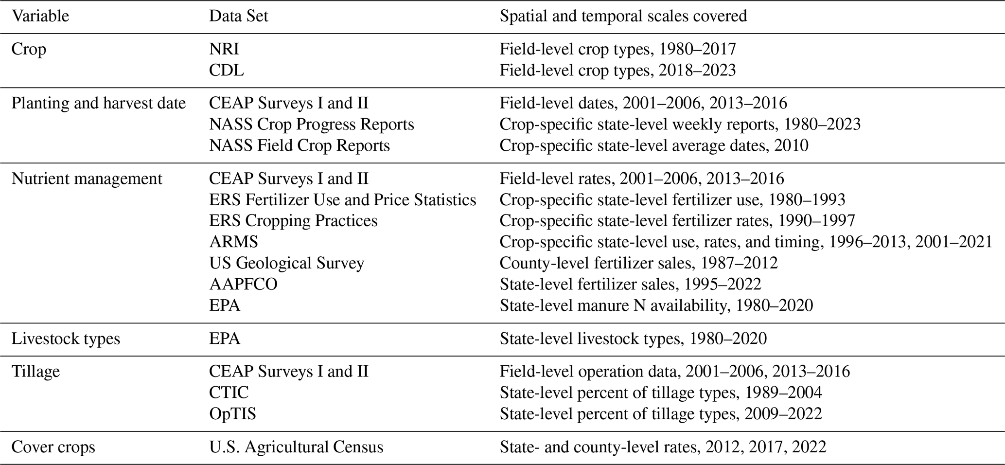
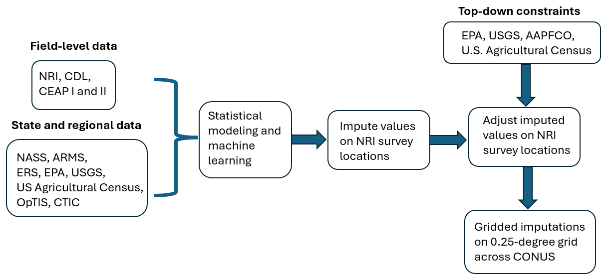
Figure 1Data assimilation process for creating the gridded imputations of agricultural land management practices.
Our agricultural land management activity data set focused on major crops including corn, soybeans, cotton, sorghum, wheat, barley, and oats. We imputed agricultural land management practices on the NRI sample and then aggregated the sample to a 0.25° grid to create the wall-to-wall spatio-temporal product presented here. In Sect. 3.1, we describe the data and statistical methods used to impute each of the management activities on the NRI sample. Some of the techniques rely on gradient boosted modeling (GBM), described in Appendix B, and Markov transition matrices, described in Appendix C. In Sect. 3.2, we describe the construction of the gridded data product.
3.1 Management Activity Imputations
3.1.1 Planting and Harvest Dates
We imputed planting and harvest dates for each NRI survey location using data from NASS crop progress reports (USDA, 2024), NASS field crop reports (USDA, 2010), and CEAP data (NRCS, 2012, 2022). NASS crop progress reports were published from 1980–2023 and contained the crop planting progress by week as a percent of cropland acres. Data were stratified by state and crop, and included corn, soybeans, cotton, sorghum, winter wheat, spring wheat, barley, and oats. Because the data for barley and oats were not stratified by season of planting (i.e. winter/spring) we elected to use the crop progress report data for winter wheat to inform winter barley and oats and the data for spring wheat to inform spring barley and oats.
Using the crop progress reports, we constructed empirical cumulative distribution functions (CDF) for the planting day of year for each crop, state, and year. At each julian day of the year, the CDF provides the percent of cropland area planted on or before that date. The CDF is zero before any crops are planted and monotonically non-decreasing until the date that all crops are planted (i.e. when progress reaches 100 %). For each state, crop, and year, we used piecewise cubic Hermite interpolation (PCHIP) in the R package signal (signal developers, 2023) to interpolate the CDF and create a continuous distribution between the minimum and maximum dates provided by the crop progress reports. PCHIP is a non-linear interpolation method that enforces the monotonicity of the CDF.
We constructed CDFs from the 0.10 quantile (the first date on which at least 10 % of the cropland area was planted) to the 0.90 quantile for each state, crop, and year. For some state-crop-year combinations (<20 %), the full CDF could not be constructed and we borrowed planting date progress information from the closest year for the same state and crop. For less than 10 % of the NRI sample, we were unable to construct a planting date CDF, so we simulated the distribution using data from NASS field crop reports (USDA, 2010). Specifically, we simulated planting dates using a Normal distribution with mean set to the median of the planting date range listed for the state and crop in the field crop reports and standard deviation set to the length of planting date range divided by 6. These metrics were chosen because 99.7 % of the data in a Normal distribution fall within 3 standard deviations of the mean. Hence, our simulation should capture nearly the entire range of plausible planting dates.
The NRI sample did not provide the season (winter/spring) of planting for small grains; however, this information was critical to our imputation approach as it affects several land management practices including planting and harvest dates, tillage, and cover crop adoption. Therefore, we used the CEAP data, with known planting dates, to predict the season of small grain planting on survey locations in the NRI sample. We classified small grain CEAP points into winter grain or spring grain based on their planting date, and modeled the season indicator (i.e. winter =1, spring =0) using a GBM with predictor variables CEAP region, state, MLRA, latitude, longitude, crop, previous crop, soil texture class, and soil texture group. We then used the fitted GBM to predict the season of planting for small grains in the NRI sample.
Using the planting date CDFs described above, we created probability distribution functions (PDFs) of planting date for each state, crop, and year. We imputed planting dates on the NRI sample by randomly sampling from the PDF corresponding to the state, crop, and year for each survey location.
We imputed harvest dates using NASS average dates to maturity for each crop (USDA, 2010). We used state-level data where possible and CEAP region or national data if needed. The average days to maturity were added to the imputed planting dates to impute the harvest dates for each crop. Planting and harvest dates were subsequently adjusted to ensure that harvest took place before the next planting event at the same location.
3.1.2 Nutrient Management
For each NRI survey location, we imputed the annual rates (kg N ha−1) and application timing of synthetic N fertilization and manure amendment, as well as the animal type for the manure. For each state, crop, and year, we first predicted the percentage of cropland area managed with synthetic fertilizers and manure amendments, and then randomly selected NRI survey locations to receive the fertilizer and/or manure amendments. We then imputed the application rate and timing for each survey location.
We used data from ARMS (USDA-ERS, 2020) and ERS (Taylor, 1994; USDA-ERS, 1997) to predict the percentage of cropland area managed with synthetic N fertilizer and manure amendments for corn, cotton, soybeans, and wheat. For each state from 1980–2023, we predicted the percentage of treated cropland area using GBMs that were trained on the ARMS data with state, crop, and year as predictor variables. The predicted percentages were restricted to between 0 and 100. We then randomly selected NRI survey locations to receive fertilizer and manure amendments based on the predicted percentages for the respective state, crop, and year.
To impute nutrient application rates, we first used state-level data to establish long-term trends in crop-specific rates in each state, which were then used in the field-level analyses to maintain consistency over the time series. We used GBMs to construct the baseline trends for both synthetic N fertilizer and manure amendment. For synthetic N fertilizer, the training data included state-level crop-specific fertilization rate data from ARMS (USDA-ERS, 2020) and ERS (Taylor, 1994; USDA-ERS, 1997), and the predictor variables in the GBM were state, crop, and year. For manure amendments, the training data set combined manure amendment rate data from ARMS (USDA-ERS, 2020) and manure N availability data from EPA (EPA, 2024), and the predictor variables were state, crop, year, and relative manure N available for application to soils (i.e. total manure N available for the state and year divided by the maximum amount available for the state over the time series). We used the fitted GBMs to predict average state-level fertilization and manure amendment rates for each crop from 1980–2023.
We modeled the field-level CEAP data (NRCS, 2012, 2022) to impute synthetic N fertilization and manure amendment rates on the NRI survey locations. First, we calculated residual differences between rates at CEAP survey locations and the predicted crop-specific state-level average rates generated as described above. We centered the residual differences on their mean within a state, crop, and year. Then, separately for fertilizer and manure, we modeled the centered residuals using GBMs with the following predictor variables: CEAP region, MLRA, state, crop, previous crop, latitude, longitude, flood class, irrigation, soil texture class, soil texture group, minimum slope of the land, maximum slope of the land, and planting day of year. In the manure rate model, we also included the imputed fertilization rate as a predictor variable; hence, we imputed fertilization rates on the NRI sample before implementing the manure rate model. Using the GBMs, we predicted residual rates for each NRI survey location, which were added to the crop-specific state-level average rates to create initial imputed values of the synthetic fertilization and manure amendment rates on the NRI sample.
Synthetic fertilizer and manure amendment rates were constrained by annual totals of fertilizer sold and manure N available for agricultural land application. County-level USGS fertilizer sales data for 1987–2012 (Brakebill and Gronberg, 2017) were aggregated to the state level and combined with state-level AAPFCO data from 2013–2017 (AAPFCO, 2008-2022), and then extended to 1980–2023 using auto-regressive moving average models. We assigned average fertilization rates for unmodeled crops (vegetables, horticulture, hay, and pasture) from ARMS and NASS data (USDA-NASS, 2011, 2020). We then calculated the total amount of synthetic N fertilizer (kg) applied to all crops in each state and year. The percentage of over-application was computed as
for each state and year. Rates at each NRI survey location were reduced by the percent of over-application. The adjustment was required for 65.4 % of NRI survey locations (mean adjustment rate of 11.4 %).
Manure amendments were adjusted similarly using available manure N data (EPA, 2024), reserving a share proportional to unmodeled cropland area. Over-application for modeled crops was computed as
for each state and year. Adjustments affected 31.5 % of NRI survey locations (mean adjustment rate of 12.9 %).
Manure livestock animal types (beef, dairy, poultry, swine, horse, sheep, and biosolids) were imputed based on state-level livestock fractions for manure available for application to soils from EPA (2024). Specifically, the data were combined and linearly interpolated to fill in missing years from 1980–2020. The 2020 state-level fractions were used for 2021–2023. We predicted animal types on the NRI sample by random sampling based on the annual state-level animal type fractions. Then we calculated the C amount for each survey location receiving manure in the NRI sample using C:N ratios for each animal type. The C:N ratios were 12.60 for beef and dairy, 13.00 for biosolids, 17.40 for poultry, 13.45 for swine, 30.72 for horse, and 11.36 for sheep (USDA, 1992).
We imputed the timing of synthetic N fertilization based on four timing windows: fall (F), spring before planting (S), at planting (P), and after planting (O). Fertilization events in the fall could occur before planting a fall crop or in preparation for a spring crop. To account for split applications, we considered all combinations of the four timing windows, resulting in a total of 15 timing categories (F, S, P, O, FS, FP, FO, SP, SO, PO, FSP, FSO, FPO, SPO, FSPO). State-level ARMS data on the proportion of cropland area fertilized during each timing category and the percent of fertilizer applied in each timing window for split applications were available every 4–5 years from 2001–2021 for corn, cotton, winter wheat, and spring wheat. We used linear interpolation to gap-fill missing data and first and last value carried backward and forward, respectively, to extend the time series to 1980 and 2023. Using the interpolated timing category proportions, we randomly selected a timing category for each survey location receiving fertilizer in the NRI sample. Conditional on the timing category, we split the application rate among the timing windows based on the interpolated split application percents (e.g. conditional on timing category of FSP, we split applications among F, S, and P).
We imputed timing of manure amendments into fall, spring, and after planting. Manure amendments were assumed to be applied at only one time based on data available from ARMS. We gap-filled state-level ARMS data on the percent of manure applied in each timing window for corn, cotton, winter wheat, and spring wheat using the same methods as described above. Using the interpolated percentages, we randomly selected a manure application timing window for each survey location receiving manure amendments in the NRI sample.
Due to data limitations, application rate data for sorghum was borrowed from corn and application rate data for barley and oats was borrowed from wheat. For soybeans, we assumed all fertilizer was applied at planting and all manure was applied in spring before planting. Our data set is restricted to soil management and does not provide information on the collection, storage, or handling of manure.
3.1.3 Tillage
We imputed tillage practices from 1980–2023 in two parts in order to capture broad tillage system types as well as specific information on tillage intensity. First, we imputed five-year tillage system types as no-till (N), reduced till (RT), or full till (FT, also identified as conventional till in the surveys). This information captures the prevailing tillage systems, and is classified based on the most intensive tillage practice in the five-year period. Second, we imputed specific annual tillage intensity patterns conditional on the imputed five-year tillage system types.
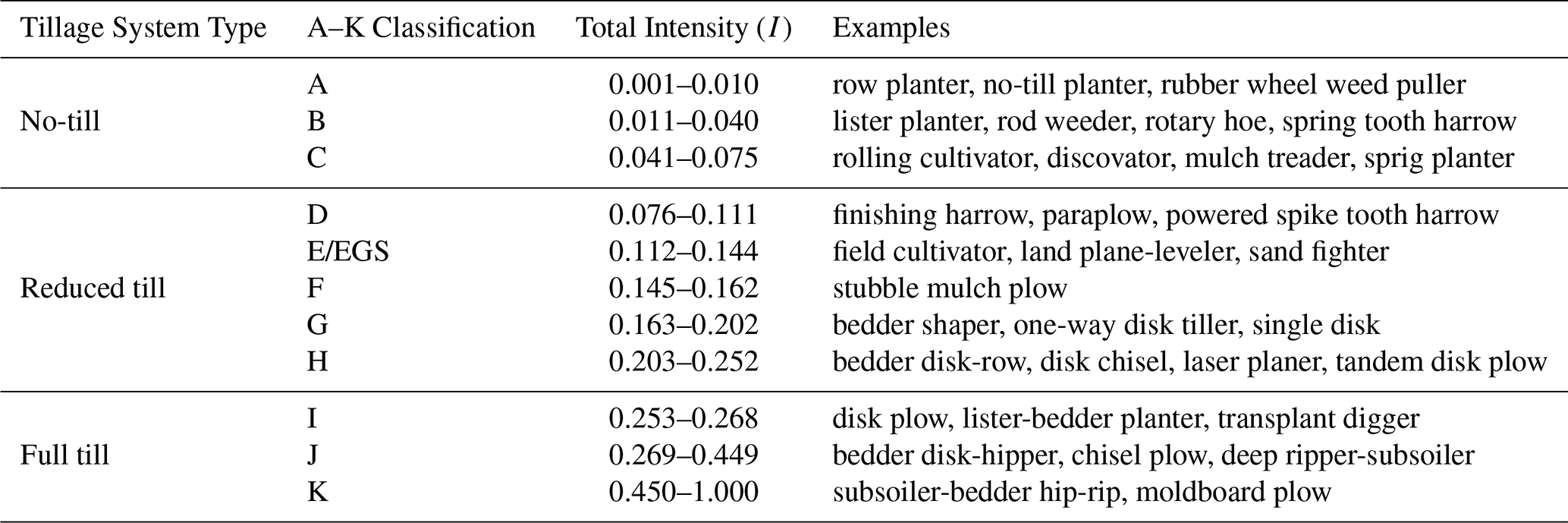
CTIC and OpTIS data provided information on broad tillage systems (i.e., NT, RT, and FT), while CEAP provided detailed information on the date, machine type, mixing efficiency, and tillage depth for all tillage implements used at each CEAP survey location. We used data on tillage systems from all three data sets to classify 5-year tillage systems, and then used implement data from CEAP to assign specific tillage intensity patterns to each year in the 5-year block. We classified CEAP data into the broad tillage systems to relate the CEAP survey to CTIC and OpTIS. To do so, we assigned each tillage implement to one of five operating windows: field preparation (≥ 56 d before planting), before planting (7–55 d before planting), at planting (0–6 d before planting), after planting (1 d after planting to 1 d before harvest), and post harvest (on or after harvest). After grouping the tillage implements into operating windows, we calculated the total intensity (I) for each window to a 30 cm depth using the following equations from Ogle et al. (2024):
where Tt is the tillage intensity for implement in a single operating window at a specific survey location, Et is the mixing efficiency for implement t, and Dt is the tillage depth for implement t. The total intensities for each operating window were classified as categorical variables (A, B, …, K) based on the relationships given in Table 2 (Ogle et al., 2024). We added a customized intensity level, EGS, for cases when the tillage intensity Eq. (3) resulted in an intensity after planting that would practically kill the growing crop (i.e. more intense than C). We assumed these events were due to weeding. Each survey location was then assigned an annual tillage system type (NT, RT, or FT) based on the most intense A–K classification among all operating windows in that year (Table 2).
Table 2Tillage system types, A–K classification, intensity mapping, and implement examples.
We combined the tillage system data from CEAP, CTIC, and OpTIS, and based tillage system imputations on crop groups defined by row crops (corn, soybeans, and sorghum), low residue crops (cotton), and small grains (wheat, barley, oats). Separately for each crop group, we modeled the log ratio of NT to FT percentages and the log ratio of RT to FT percentages using linear models with the following predictor variables: CEAP region, state by CEAP region, a quadratic function of year, and an interaction between CEAP region and the quadratic function of year. Using the linear models, we predicted the percentage of 5-year tillage system types for each crop group from 1980–2023.
Next, we imputed five-year tillage system types on the NRI sample. Starting with the 2021–2025 block (which was a partial block consisting of years 2021–2023), we used the predicted percentages calculated above to randomly select NRI survey locations to assign NT, RT, and FT five-year tillage systems. We imputed tillage system types for survey locations in the remaining time-blocks using a Markov transition model (See Appendix C for more information).
After assigning five-year tillage systems, we imputed the annual tillage intensity patterns using the A–K classifications in each operating window derived from the CEAP data. For example, possible intensity patterns include: (1) A at planting, (2) J before planting and E at planting, or (3) I at field preparation, I before planting, and B at planting. We used a hot-deck imputation approach (Andridge and Little, 2010) stratified by CEAP donor pools to impute annual tillage intensity patterns on the NRI sample. The CEAP donor pools were constructed by year (CEAP survey 1 was used for 1980–2008 and CEAP survey 2 for 2009–2023), CEAP region, crop (or crop group if the specific crop was not available), and five-year tillage system type. We matched each NRI survey location to a CEAP donor pool, then randomly selected a tillage intensity pattern from the donor pool to represent the annual tillage intensity pattern at that NRI survey location. This approach captured rotational tillage systems where the field may be occasionally cultivated with a more intensive tillage practice to control the weeds or address soil compaction that occurs with less intensive systems (Lu et al., 2022a). We enforced constraints so (1) there were not two fall tillage events (e.g. post harvest tillage after a spring crop and then fall field prep tillage before the next crop) and (2) at least one year in the five-year block had the same tillage system as the five-year tillage system type.
3.1.4 Cover Crops
We imputed cover crops on the NRI sample as a binary indicator of adoption from 1990–2023 using state- and county-level data from the 2012, 2017, and 2022 U.S. Agricultural Census. We assumed no cover crop adoption prior to 1990. First, we estimated a state-level trend in cover crop adoption from 1990–2023. To do so, we calculated the percentage of harvested cropland area with cover crop adoption in each state and year based on the Census data, and then constructed a linear model to predict the annual state-level percentage of cover crop adoption in the NRI sample for 1990–2023. The predictor variables used in the linear model were state, year, and an interaction term between state and year to allow for state-specific temporal trends. The linear model enforced the assumption of increasing cover crop adoption over time. Second, we used the state-level trend to complete the time series in the county-level data. Working backwards from year 2012 to year 1990, we calculated the year-to-year ratio of cover crop adoption for each state, and applied this ratio to the county-level data to extrapolate the county-level cover crop adoption rates. We applied a similar method to extrapolate county-level cover crop adoption for 2023. For years 2013–2016 and 2018–2021, which were within the range of the Census data available, we used linear interpolation within each county to estimate the county-level cover crop adoption. We filled missing county-level data with the corresponding state-level data.
We imputed cover crops on the NRI sample by first randomly selecting NRI survey locations in 2023 to assign cover crops using the county-level estimates derived above. We then imputed backward to 1990 using a Markov transition model (See Appendix C). We constrained the algorithm so that cover crops and cash crops (e.g. winter grains or other fall planted crops) were not planted at the same time.
3.2 Creating the Gridded Product
We aggregated the agricultural land management activity data from the NRI survey sample to a 0.25° grid to preserve confidentiality of the NRI survey locations. Individual NRI survey locations were weighted based on their survey area weight, which was provided by the NRI. Hence, the contribution of each NRI survey location to the aggregated grid cell was proportional to its weight. We produced six imputations of management activities in our analysis to capture the variability in predicted management activities at the field level. This variability is based on random sampling inherent in the statistical algorithms used to impute each management practice. Measures of variation in the gridded data set include both variability among and within the NRI survey locations in each grid cell. The gridded data are in NetCDF format and are available for download from Dryad (Hoskovec et al., 2026).
For each grid cell from 1980–2023, we reported the 0.10, 0.25, 0.50, 0.75, and 0.90 quantiles of planting and harvest dates by crop; the mean and between-imputation standard deviation of synthetic N fertilizer and manure N and C application rates in each timing window by crop; the proportion of manure animal types; the mean and between-imputation standard deviation of the proportion of annual tillage system types by crop group (low residue, small grains, and row crops); the proportion of A–K classes in each operating window; and the mean and between-imputation standard deviation of the proportion of cover crop adoption. To preserve the confidentiality of the NRI survey locations and associated field information, gridded data were suppressed if there were fewer than three NRI survey locations within the grid cell. Notably, grid cells with fewer than three NRI survey locations were areas with little cropland and contribute minimally to larger regional patterns in cropland management. We did not provide follow-up interpolations for the suppressed data.
We provide a detailed evaluation of the imputations in Appendix D. Briefly, our survey location-level imputations closely match predictions from statistical models and align with the observed data when moderate to high amounts of data are available. Where data are scarce, the differences between predicted values (e.g. predictions from linear models, GBMs or Markov transition models) and observed values are large, leading to larger differences between imputed values and observed values. Hence, increasing temporal and spatial data availability will lead to more accurate inferences on field-level management activities in future products.
We describe the key results for each imputed management activity in the following sections. Supplementary results are available in Appendix E.
4.1 Planting Date
National temporal trends in imputed planting dates varied by crop (Fig. 2). Between 1980 and 2023, there were no overall changes in median planting dates across CONUS for corn (, , p-value =0.65), sorghum (β1=0.03, .02, p-value =0.58), or winter wheat (.02, .01, p-value =0.45). Despite no overall trend, there was high inter-annual variability in planting dates for corn. Between 1980 and 2023, soybeans were planted an average of 12 d earlier (.27, R2=0.32, p-value < 0.01), while cotton (β1=0.27, R2=0.56, p-value < 0.01) and spring wheat (β1=0.20, R2=0.09, p-value =0.03) were planted an average of 12 and 9 d later, respectively. The planting date patterns for barley and oats were similar to those for wheat.
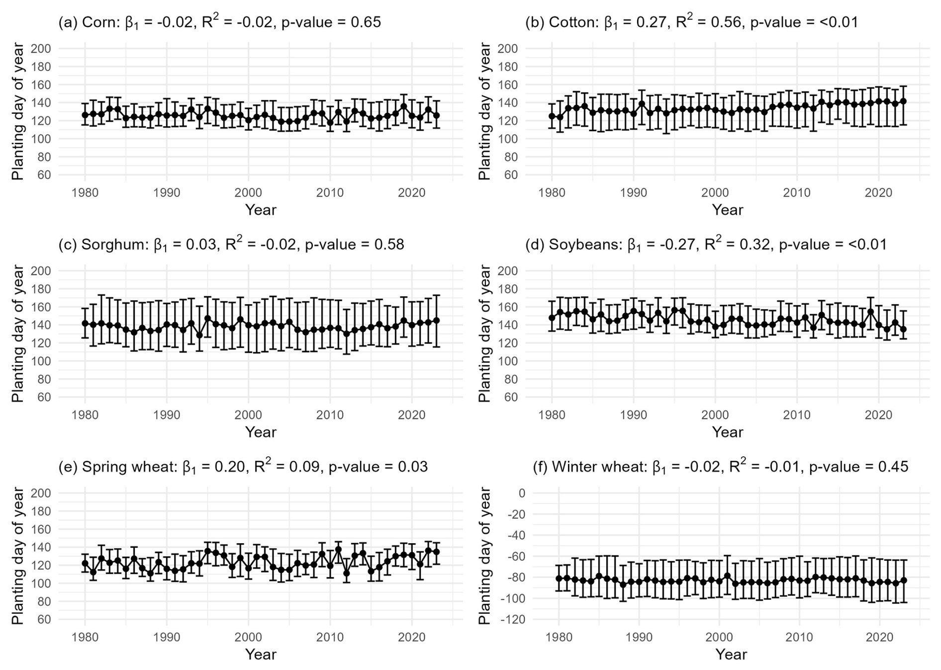
Figure 2Distribution of imputed planting dates by crop over time from 1980–2023. Panels (a)–(f) show the median, 0.10 quantile, and 0.90 quantile for the imputed planting dates for corn, cotton, sorghum, soybeans, spring wheat, and winter wheat, respectively.
4.2 Nitrogen Management
We created gridded maps of crop-specific synthetic N fertilizer and manure N application rates for 2023. Most synthetic N fertilizer was applied to corn, particularly in the Midwest (Fig. 3). The national average N fertilizer rate for corn was 122.5 kg N ha−1 in 2023. Cotton, spring wheat, and winter wheat received moderate rates of fertilizer application, with national average rates in 2023 of 90.1, 79.1, and 68.9 kg N ha−1, respectively. For cotton, rates were higher in the Southeast, and for winter wheat, rates were higher in the northern Midwest and California coastal regions. Soybeans received very little synthetic N fertilizer, with an average rate in 2023 of 9.7 kg N ha−1.
Manure amendment rates were much lower than synthetic N fertilizer rates, but still generally highest for corn in the Midwest (Fig. 4). The national average manure N amendment rate for corn in 2023 was 20.7 kg N ha−1. The northeast Atlantic regions also had higher manure application rates compared to other areas of CONUS. Some manure was applied to soybeans (2023 national average rate = 8.4 kg N ha−1), but very little was applied to cotton or wheat (2023 national average rates < 6.2 kg N ha−1).
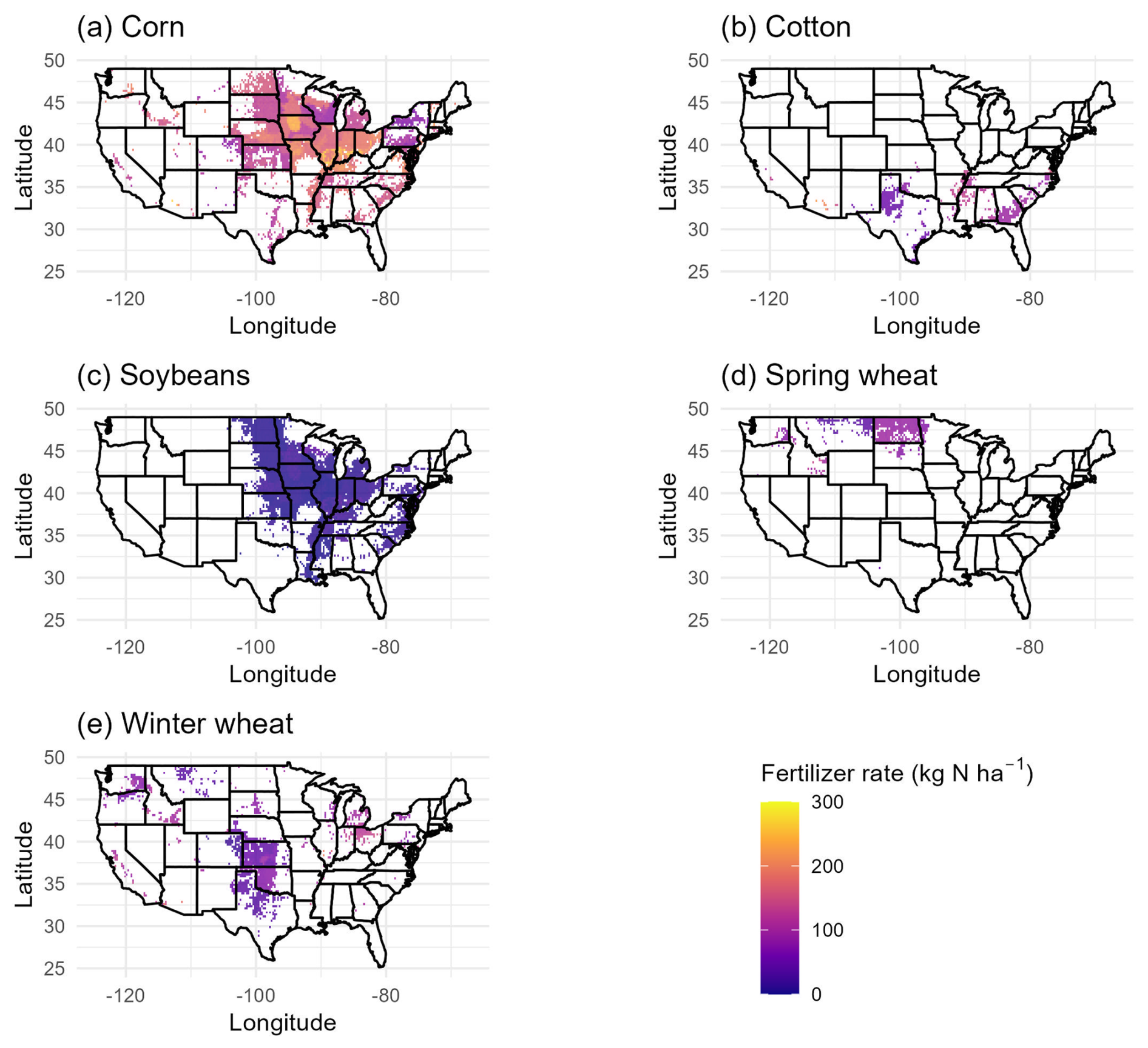
Figure 3Average imputed synthetic fertilizer rates (kg N ha−1) across CONUS in 2023 for corn, cotton, soybeans, spring wheat, and winter wheat.
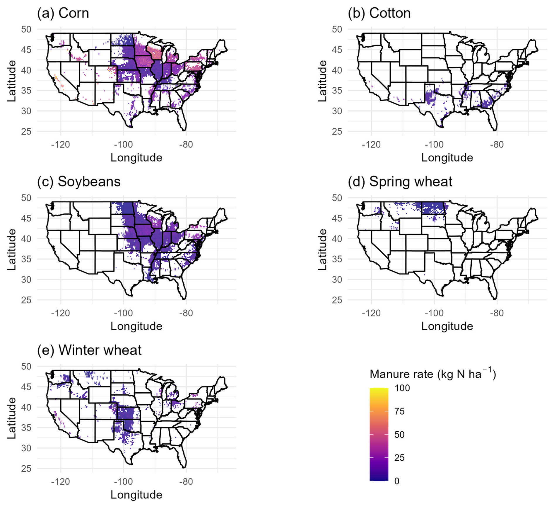
Figure 4Average imputed manure amendment rates (kg N ha−1) across CONUS in 2023 for corn, cotton, soybeans, spring wheat, and winter wheat.
Application rates changed over time. Total synthetic N fertilizer rates increased from 1980 to 2000 and then remained relatively stable from 2000 to 2020 (Fig. 5). Specifically, from 1980–2023, average synthetic N fertilizer application rates increased from 122.5 to 150.9 kg N ha−1 for corn, 63.8 to 90.1 kg N ha−1 for cotton, 6.8 to 9.7 kg N ha−1 for soybeans, 34.8 to 29.1 kg N ha−1 for spring wheat, and 53.4 to 68.9 kg N ha−1 for winter wheat. Corn was mostly fertilized in the spring or after planting, though fall application rates for corn increased over time. Applications for winter wheat were highest in fall, and applications for cotton were highest after planting. Spring wheat applications generally occurred in spring before planting or at planting. Data on timing of fertilizer applications was only available every 4–5 years between 2001 and 2021. Hence, these results reflect state-crop-level long-term trends during this time period; trends before 2001 reflect the 2001 data.
Imputed manure N application rates showed a different pattern from synthetic N fertilizer, with rates being relatively stable from 1980 to 2000, then increasing slowly from 2000 to 2020 (Fig. 6). Between 1980 and 2023, average manure N amendments increased from 14.9 to 20.7 kg N ha−1 for corn, 4.2 to 6.1 kg N ha−1 for cotton, 3.1 to 8.4 kg N ha−1 for soybeans, 3.2 to 6.2 kg N ha−1 for winter wheat, and decreased from 2.3 to 1.5 kg N ha−1 for spring wheat. Most manure was applied in fall or spring before planting, while very little manure was applied after planting. Towards the later part of the time series, there were increases in spring manure rates for corn, soybeans, and cotton, and increases in fall manure rates for corn and winter wheat. Imputed fertilizer and manure N application rates and timing for sorghum were similar to those for corn, and imputed rates for barley and oats were similar to those for wheat.
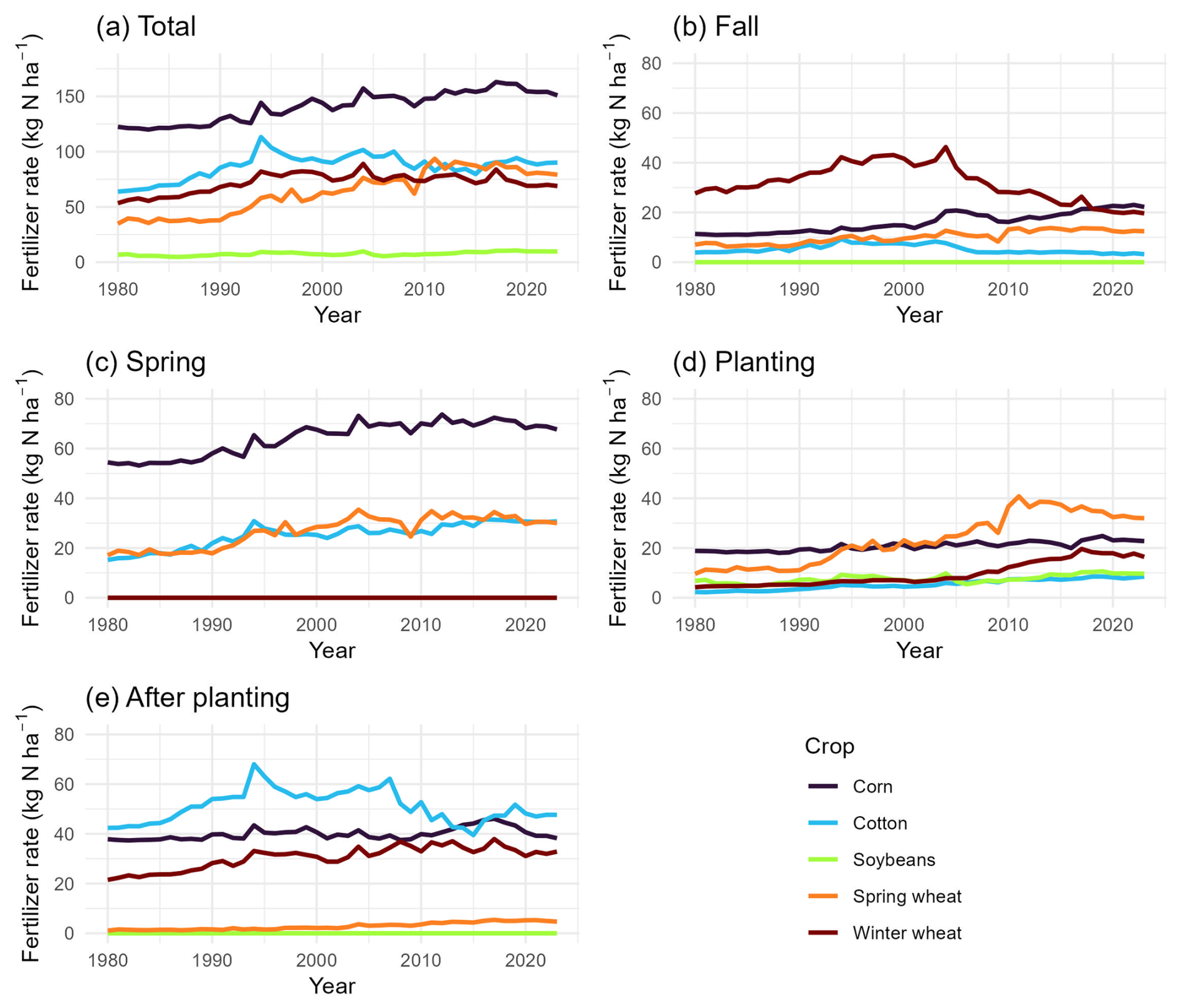
Figure 5Average imputed synthetic fertilizer rates (kg N ha−1) in each timing window (total, fall, spring, planting, and after planting) from 1980–2023 for corn, cotton, soybeans, spring wheat, and winter wheat.
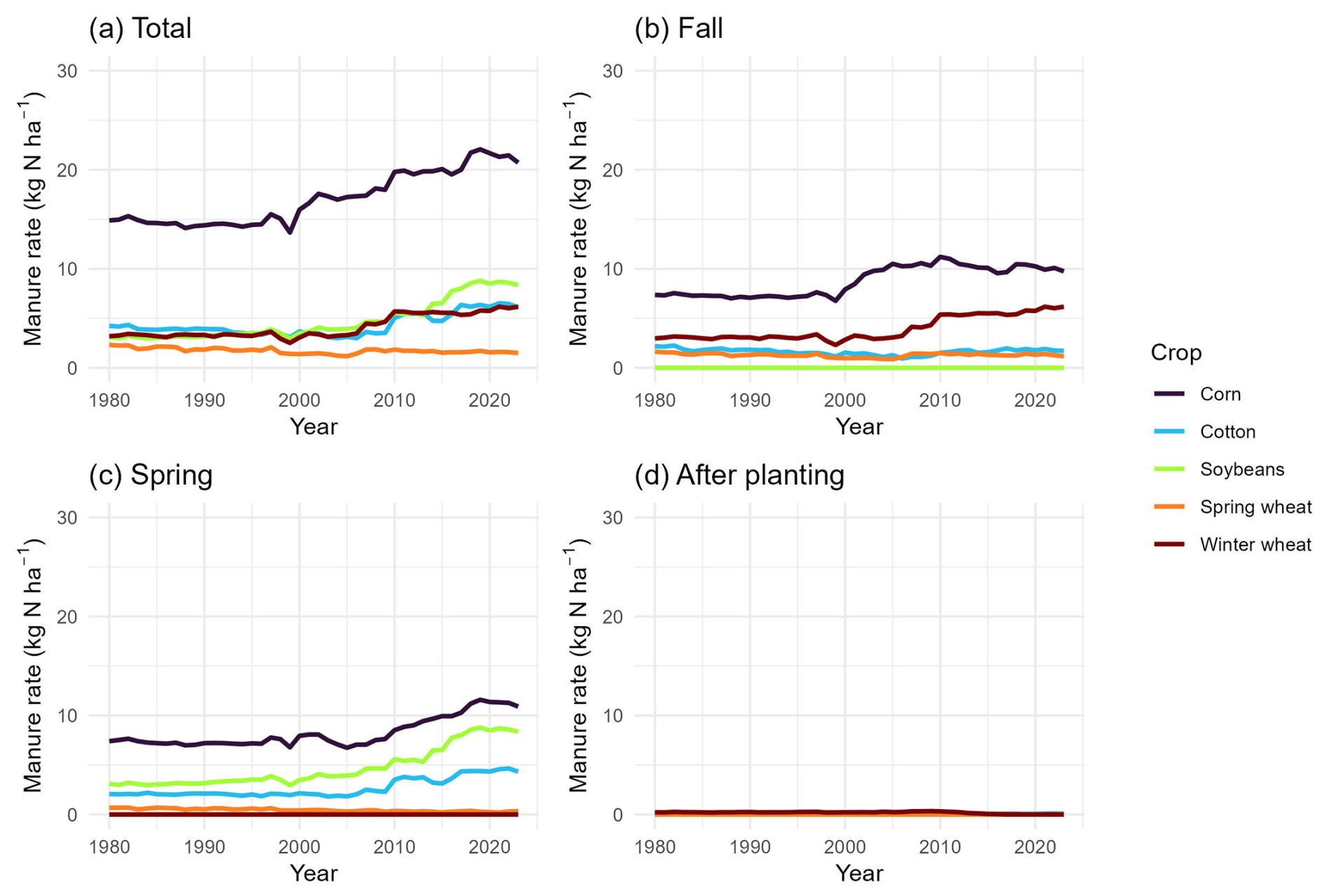
Figure 6Average imputed manure amendment rates (kg N ha−1) in each timing window (total, fall, spring, and after planting) from 1980–2023 for corn, cotton, soybeans, spring wheat, and winter wheat.
The percent of manure amendments coming from each animal type changed slightly over time, with most manure coming from dairy, swine, beef, and poultry (Fig. 7). The proportion of manure from dairy decreased from 1980–2023, while the proportions from the other animal types increased.
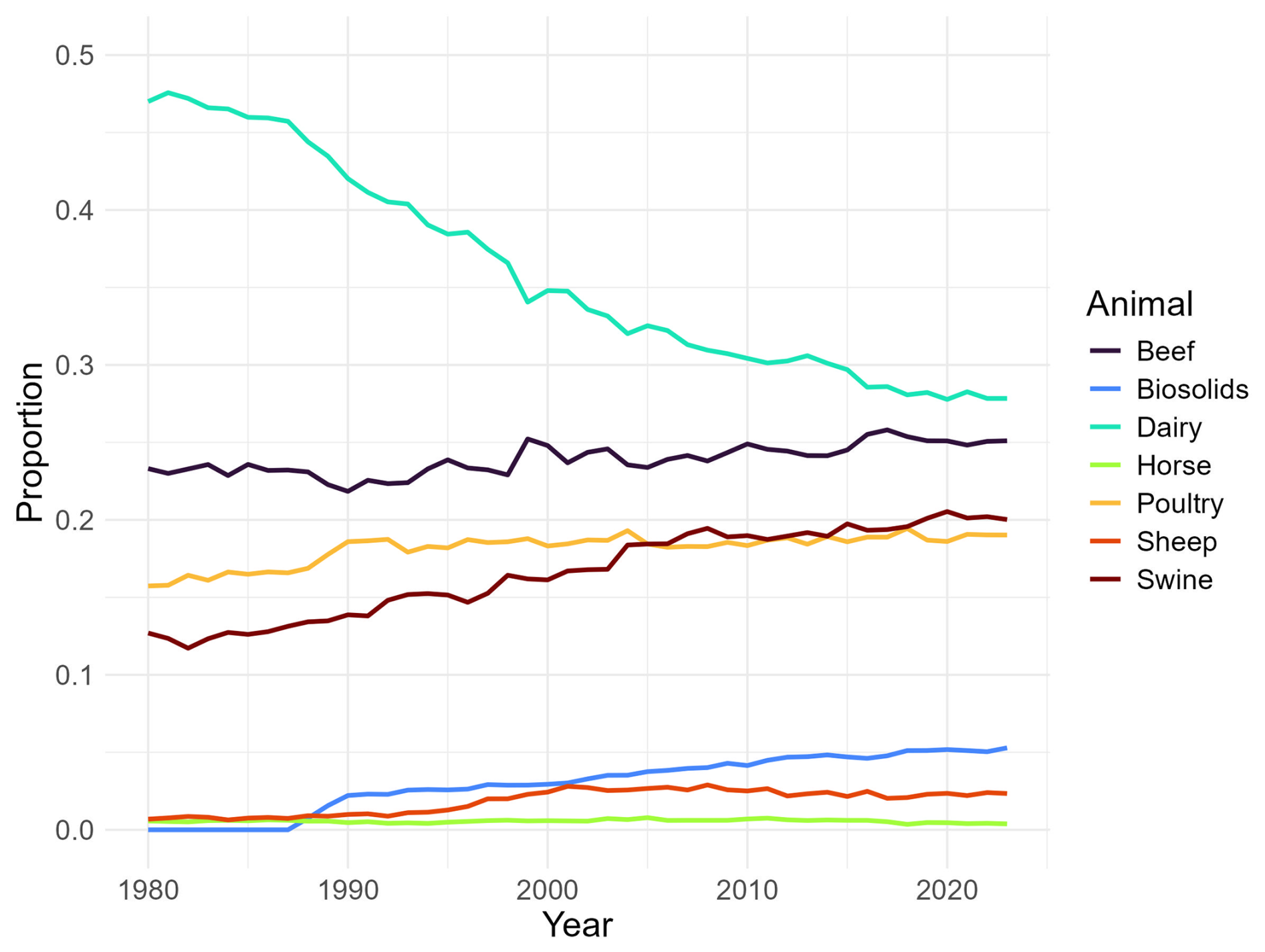
Figure 7National trends from 1980–2023 in the percent of manure amendments from each animal type.
4.3 Tillage
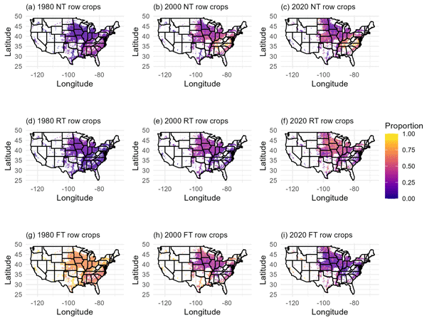
We created gridded maps of the proportion of each tillage system type by crop group across CONUS for 1980, 2000, and 2020. We discuss the results for row crops in the main text and include the results for low residue crops and small grains in Appendix E. Between 1980 and 2020, the proportion of row crop cropland area managed with NT tillage systems increased from 17.8 % to 37.0 % and the proportion of cropland area managed with RT tillage systems increased from 13.5 % to 40.0 %. The proportion of cropland area managed with FT tillage systems decreased from 72.8 % in 1980 to 25.6 % in 2020 (Fig. 8). The percentages do not sum to exactly 100 % due to data suppression. The most accelerated shift towards NT systems occurred in the East Central region of CONUS. The North Central, Midwest, and Northeast regions had the most rapid adoption of RT systems. While the primary trends for NT demonstrate increasing adoption over time, there are some notable exceptions towards the latter part of the time series in which the area managed with NT declines slightly while the area managed with RT increases. FT systems remained common in the Northwest, Southwest, and California Coastal regions, but decreased in all other areas of CONUS. Tillage system patterns were similar for low residue crops and small grains (Figs. E1 and E2).
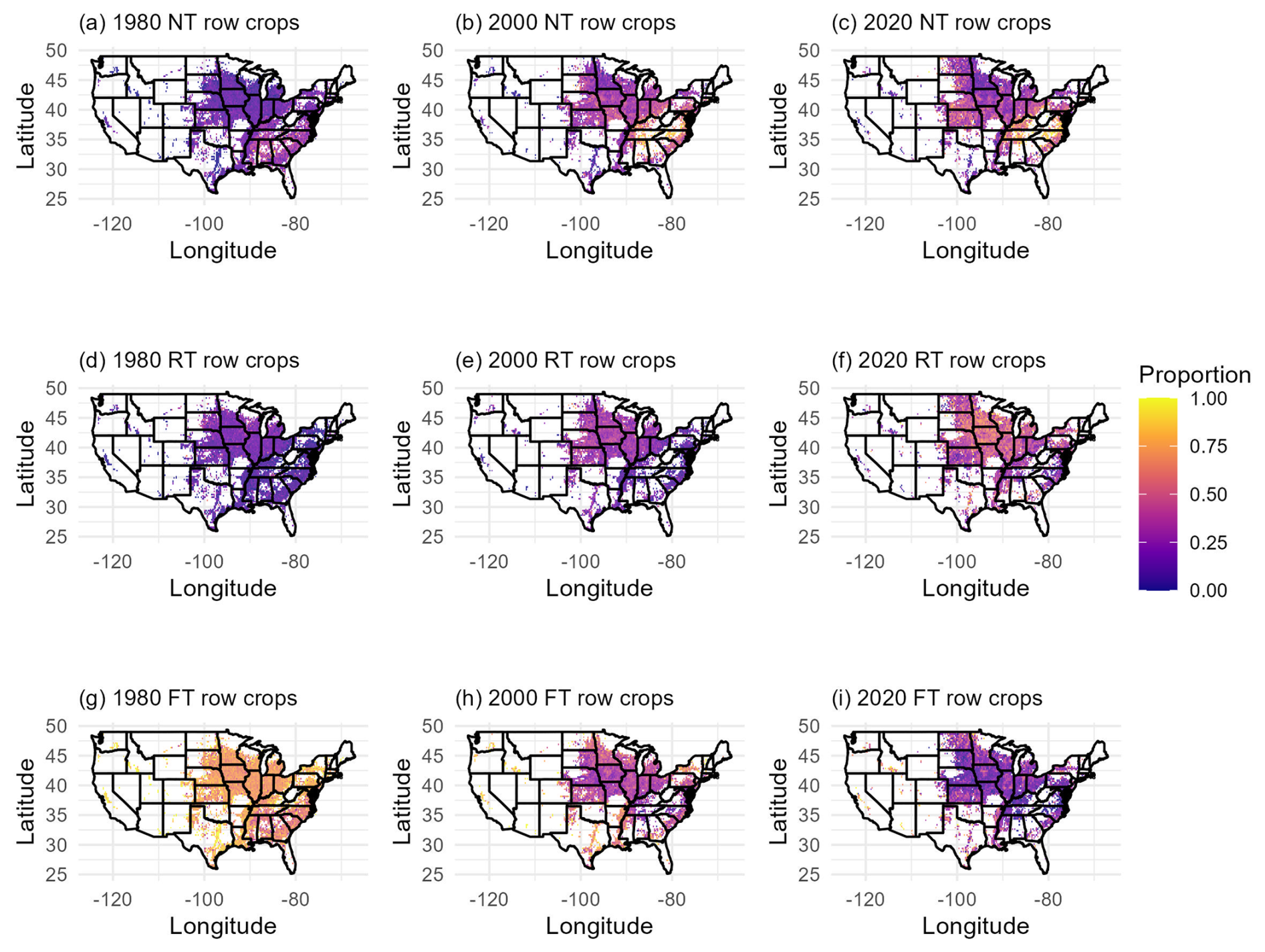
Figure 8Proportion of row crop (corn, sorghum, soybeans) cropland area managed with each tillage system type (FT = full/conventional tillage, RT = reduced tillage, NT = no tillage) across CONUS for 1980, 2000, and 2020.
The distribution of specific tillage intensities varied across the operating windows (field prep, before planting, planting, after planting, and post harvest) (Fig. 9). We reported the proportion of imputed tillage intensities in each operating window across CONUS for 2023 to demonstrate this variability. Most tillage occurred at planting, and A was the most common intensity at planting, followed by B and E. More intense tillage operations (I–K intensities, which are part of FT systems) tended to occur during field prep or before planting. After planting tillage was limited to B, C, and EGS intensities, as anything more intense would pose risk to the growing crop. Little tillage occurred post harvest, but when it did, more intense operations such as J and K were most common.
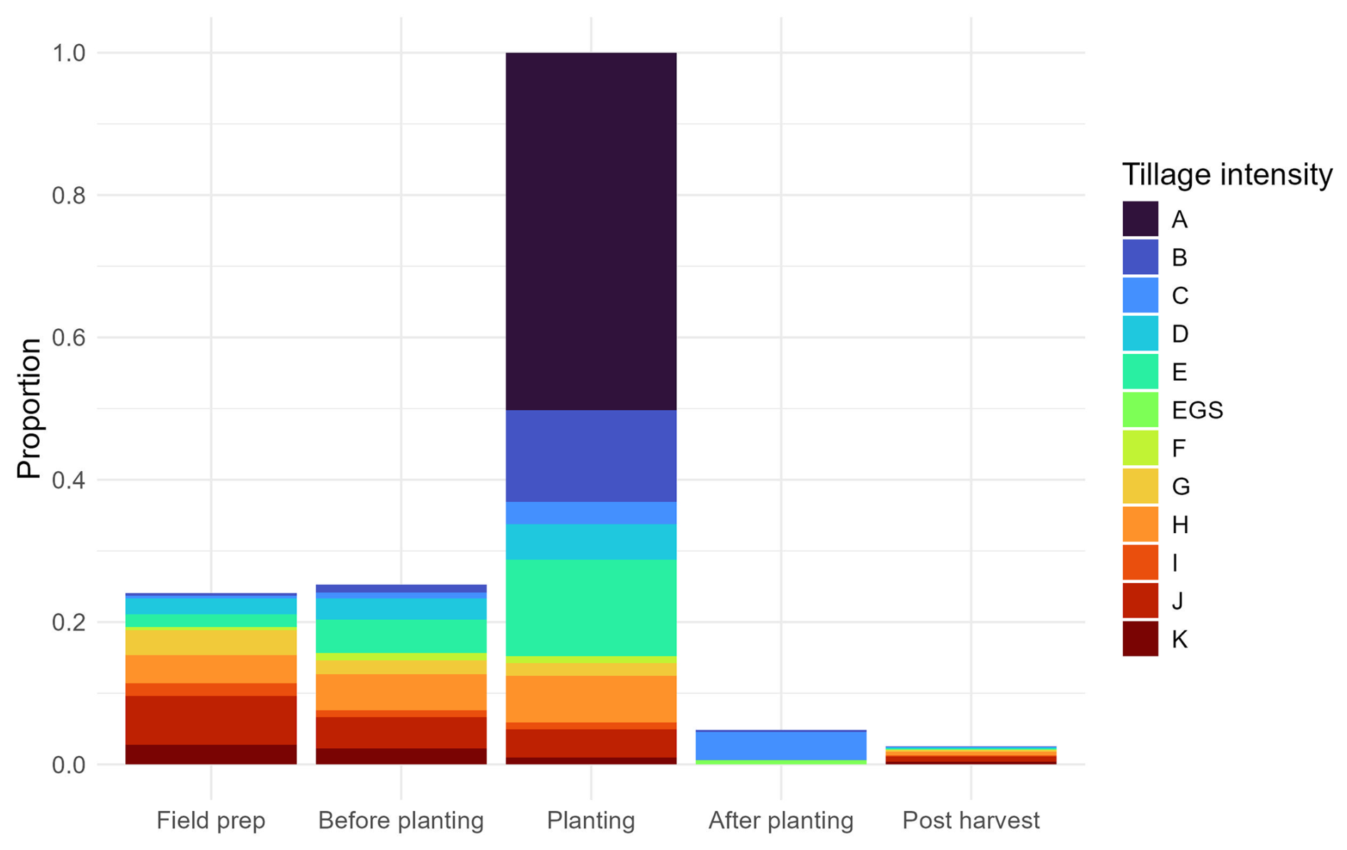
Figure 9Proportion of tillage intensities used during each tillage operating window in 2023 across all crops. Tillage intensities increase from A to K. The EGS tillage intensity is specific to the growing season, representing cultivation that is more intense than C but does not kill the growing plant (e.g. between-row weeding).
4.4 Cover crops
Cover crop adoption was limited from 1990–2000, appearing at first only in the Northeast, and then increased across CONUS from 2000 to 2020 (Fig. 10). The Northwest Non-Coastal, Southwest Non-Coastal, Northern Plains, and Southern Plains regions had the smallest increase in cover crop adoption, reaching only 1.09 % to 2.77 % adoption by 2020. The Coastal regions, North Central and Midwest, South Central, and Lower Mississippi and Texas Gulf Coast regions saw greater adoption, reaching 3.53 % and 5.59 % by 2020. The Northeast, East Central, and Southeast Coastal Plains had the highest adoption, reaching almost 13 % cover crop adoption by 2020 (Table E1).
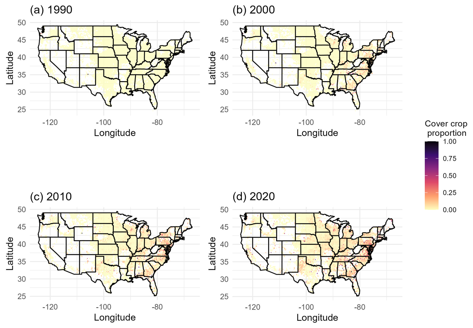
Figure 10Proportion of cropland area with cover crop adoption in each grid cell for 1990, 2000, 2010, and 2020.
We created a wall-to-wall spatial data set of agricultural land management practices from 1980–2023. Our results are comparable to other data products on spatial and temporal patterns in agricultural land management practices for CONUS. Our work also presents novelty and extensions to previous products.
Sacks and Kucharik (2011) found similar trends towards earlier planting dates for soybeans, with an average shift of −0.49 d yr−1, resulting in a 12 d earlier shift in planting from 1981 to 2005. We also found a significant trend toward earlier planting dates for soybeans, but our average shift was only −0.27 d yr−1 from 1980–2023. While Sacks and Kucharik (2011) demonstrated a trend significantly different from 0 for corn, we did not find an overall change in planting dates for corn from 1980–2023. In both analyses, high inter-annual variability in planting dates existed. Sacks and Kucharik (2011) used a similar approach involving NASS crop progress reports and PCHIP interpolation. However, because their analysis focused on a shorter time period, they observed a notable shift in planting dates for both corn and soybeans, whereas our analysis over a longer time span revealed a more moderate overall trend for soybeans and no trend for corn.
Regarding N management, Lu et al. (2022b) found increases in chemical N fertilizer application rates from 1900–2019, with more rapid increases from the 1960s to 1980s and slower increases since the 1980s. In terms of spatial patterns, most chemical N fertilizer applications occurred in the Midwest, followed by the Northern Great Plains and the Southern Great Plains. We found similar trends in synthetic N fertilizer applications, where rates increased rapidly from 1980–2000 and stabilized from 2000–2023, and the highest rates were applied in the Midwest. Both our product and the N fertilizer data product used in Lu et al. (2022b), which was developed by Cao et al. (2018), were created using fertilizer application rate data from USDA Economic Research Service (USDA-ERS, 1997, 2020) and NASS (USDA-NASS, 2025). Moreover, both products incorporated fertilizer sales data from Brakebill and Gronberg (2017). Cao et al. (2018) found national N fertilizer application rates increased from 2.2 kg N ha−1 yr−1 in 1940 to 90.4 kg N ha−1 yr−1 in 2015. Although our time series starts decades later in 1980, our results align with these patterns as national average N application rates for the crops modeled in our analysis increased from 66.5 kg N ha−1 in 1980 to 82.9 kg N ha−1 in 2023. While the general trends are similar, the difference in estimated rates is likely to due to differences in the crops modeled. In addition, Cao et al. (2018) incorporated early historical N use data from Mehring et al. (1946) and used cubic spline interpolation and distance weighted imputation to gap-fill the N use surveys, whereas our data sources focused on the 1980–2023 time period and we used GBM to complete the state- and crop-level time series. Differences in methods and data sources used may drive some differences in results, although generally the results are similar and our product offers the benefit of capturing some of the uncertainty due to statistical modeling. Both our product and Cao et al. (2018) also summarized N fertilizer timing by four timing windows: fall (previous year), spring (before planting), at planting, and after planting. Cao et al. (2018) found the highest N fertilizer application rates in the spring before planting, and generally low application rates at planting. Some areas of the Midwest applied N fertilizer intensively in the fall of the previous year as well as after planting. Our results are similar, with most crops being fertilized after planting or in spring before planting, while winter grains were often fertilized in the fall. Our product also accounted for split applications, which may drive some differences in results.
Bian et al. (2021) developed a data set of manure N production and reported the highest manure N amendment rates in the Midwest and Southeast regions of CONUS, with slow but steady increases in rates over time. Our results are consistent with these spatial patterns of manure N applications, and we also demonstrated slow increases in manure amendment rates between 1980 and 2023. Both our product and that described in Bian et al. (2021) were developed using data from USDA-NASS and ARMS, but our product also leveraged field-level data from CEAP to build machine learning models for predicting rates, while Bian et al. (2021) calculated application rates based on livestock distributions and manure recoverability rates. Despite these differences in methods, we arrived at similar conclusions regarding spatio-temporal patterns of manure N amendment rates. Trends in manure animal type may be explained by patterns in farm consolidation, shifts in herd size, and improvements in efficiency of production (MacDonald, 2020; Njuki, 2022; Fancher et al., 2025).
In our product, we demonstrated increasing trends over time in NT and RT tillage systems and decreasing trends for FT tillage systems, with variability across the latitudes of CONUS. Yu et al. (2020) also showed increases in NT systems from the late 20th century until 2008, and then a noticeable decline in NT management from 2008 to present, particularly in eastern regions where NT management was practiced more often compared to other regions. Lu et al. (2022a) developed their tillage product from a commercial data set compiled by a survey company, Kynetic, but their results are consistent with the CEAP and OpTIS data sets that were used in our analysis. They concluded that declining use of NT was related to weed resistance to herbicides, and the need for occasional tillage to reduce weed infestations. Still, NT management is more common in U.S. agricultural lands than many other regions globally (Derpsch et al., 2010), with highest adoption in the Midwest and Eastern U.S. (Porwollik et al., 2019). Our product is the first data set to publish specific tillage intensities and timing patterns in addition to the tillage system types. The three tillage systems, FT, RT, and NT, do have variation in actual tillage implements, particularly RT and FT. In turn, this leads to variation in mixing of the soil and depth of tillage, which impacts the level of soil disturbance. The tillage intensities and timing categories presented in our product capture more of this variation with disaggregated categories that may be used in empirical analyses or calibrated in a model application representing the impact of tillage on soil organic carbon dynamics (e.g. Gurung et al., 2020).
For cover crops, our product shows minimal cover crop adoption from 1990–2000, slow adoption from 2000–2010, and more rapid adoption from 2010–2020. While our cover crop time series was derived from US Agricultural Census data, Zhou et al. (2022) found similar trends using satellite data and machine learning methods to model cover crop feature thresholds and identify cover crop fields. Despite recent rapid increases, both products show that cover crop adoption across CONUS is still relatively low. Zhou et al. (2022) reported cover crop adoption was at 7.2 % in the U.S. Midwest by 2021. For the crops considered in our analysis, our results show cover crop adoption in the North Central and Midwest CEAP region at 4.8 % by 2023.
Our results are limited by the data available to inform the imputations. Specifically, the ARMS data were collected every 4–5 years and only reported data on certain crops (e.g. corn, cotton, soybeans, and wheat), typically at the state level. US Agricultural Census data was available at the county level, but was not crop-specific. In some cases, only a few data points were available from these sources, resulting in an incomplete time series that was difficult to interpolate. While specific management activities and crops were available in detail in the CEAP data set, the CEAP data only spanned 2001–2006 and 2013–2016, a subset of the full time series presented here. The remotely sensed OpTIS data was only available for the central US in the first product, while the second product spanned CONUS. Other data sets were used to fill the gaps in these primary sources. Differing survey methods, intended uses, and spatio-temporal scales in the data generated levels of uncertainty that we partially captured by summarizing six imputations of the management activities in the gridded product.
We recognize that other data sets are available and could be used to supplement the data sets used here. Specifically, Falcone (2021) generated county-level estimates of nitrogen and phosphorus from fertilizer and manure for 1950–2017. State-level fertilizer use estimates were apportioned to counties using data on county-level fertilizer expenditures, and estimates of nutrients from manure were obtained from US Agricultural Census data on county-level livestock populations. However, these county-level data are not specific to croplands and may not measure exactly what we modeled (e.g. N application rates to specific crops). Our methodology was based on field-level characteristics of nearly 300 000 NRI survey locations, and we combined crop-, state- and field-level data in machine learning models to predict specific field-level rates. We captured field-level variability through multiple imputations. A limitation of our product is that we may not have adequately captured the spatial variability within a state, which may be partially explained through county-level data sets. Future improvements could combine our methodology with county-level data either as another data set for prediction or as a validation data set.
Major sources of innovation in our product lie in our use of the NRI as the sample for imputation and the CEAP data sets as detailed field-level surveys. The NRI survey provides valuable information regarding specific land use, climate, soils, topography, and irrigation, which were used to inform field-level agricultural management practices. The CEAP data includes detailed management practices for over 21 000 NRI survey locations, with specific geographic location information, allowing us to identify complex patterns in management activities with machine learning models. Previously published data sets provide valuable insights into long-term temporal trends and spatial patterns of management activities using sophisticated approaches for digitizing, up-scaling, and down-scaling data sources to appropriate spatial and temporal scales. Our product enhances the previous analyses by leveraging our access to the NRI and CEAP surveys along with publicly available data sets to predict field-level agricultural management activities on the NRI survey locations. Aggregating the imputations to the 0.25° grid then allows for dissemination of the results from these confidential surveys. As the NRI survey continues, our product can be further extended and developed to track trends in agricultural land management practices across CONUS.
The spatio-temporal data set created and analyzed in this study is publicly available from Dryad at https://doi.org/10.5061/dryad.t1g1jwtgm under public domain license (Hoskovec et al., 2026). Figures were made with R version 4.4.3 (R Core Team, 2025). Code to reproduce the figures is available at https://doi.org/10.5281/zenodo.23987242 (Hoskovec, 2026).
We combined multiple data sets and surveys to create a wall-to-wall spatial data set of agricultural land management practices for major commodity crops from 1980–2023. We statistically imputed land management activities on a national sample from the NRI and then aggregated the imputations to a 0.25° grid across CONUS. We compared our results to other published data products on agricultural land management practices. We found our results show similar trends to other published data sets, but we also expanded and incorporated novelty into our product beyond the previous data sets. This data set can also be combined with historical data before 1980 to generate a longer time series for model applications evaluating patterns further in the past, or for models that require a longer historical period to initialize state variables, such as soil organic carbon pools. We envision this data set informing land use and management studies of agricultural lands that evaluate economic dynamics, environmental impacts, food production, water quality, the carbon cycle, and/or greenhouse gas emissions.
Major Land Resource Areas (MLRAs) were an important spatial predictor in our analyses, as they characterize geographic ares by shared climate, soils, topography, water resources, and land use (Fig. A1).
We used CEAP regions as a spatial stratification level in our imputation process for several management activities (Fig. A2).
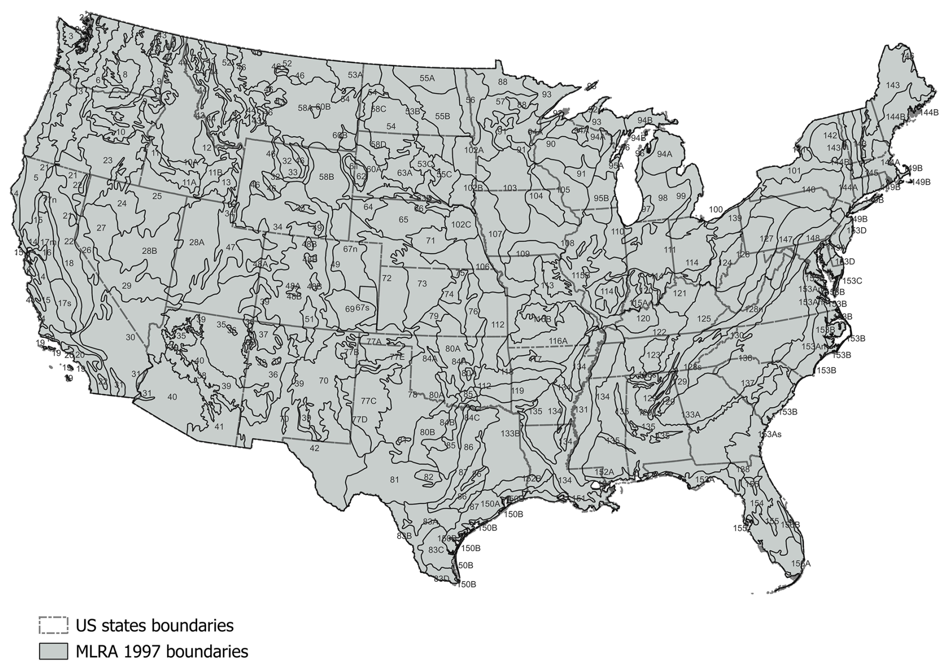
Figure A1Map of 1997 Major Land Resource Areas used in analysis as a spatial stratification variable.
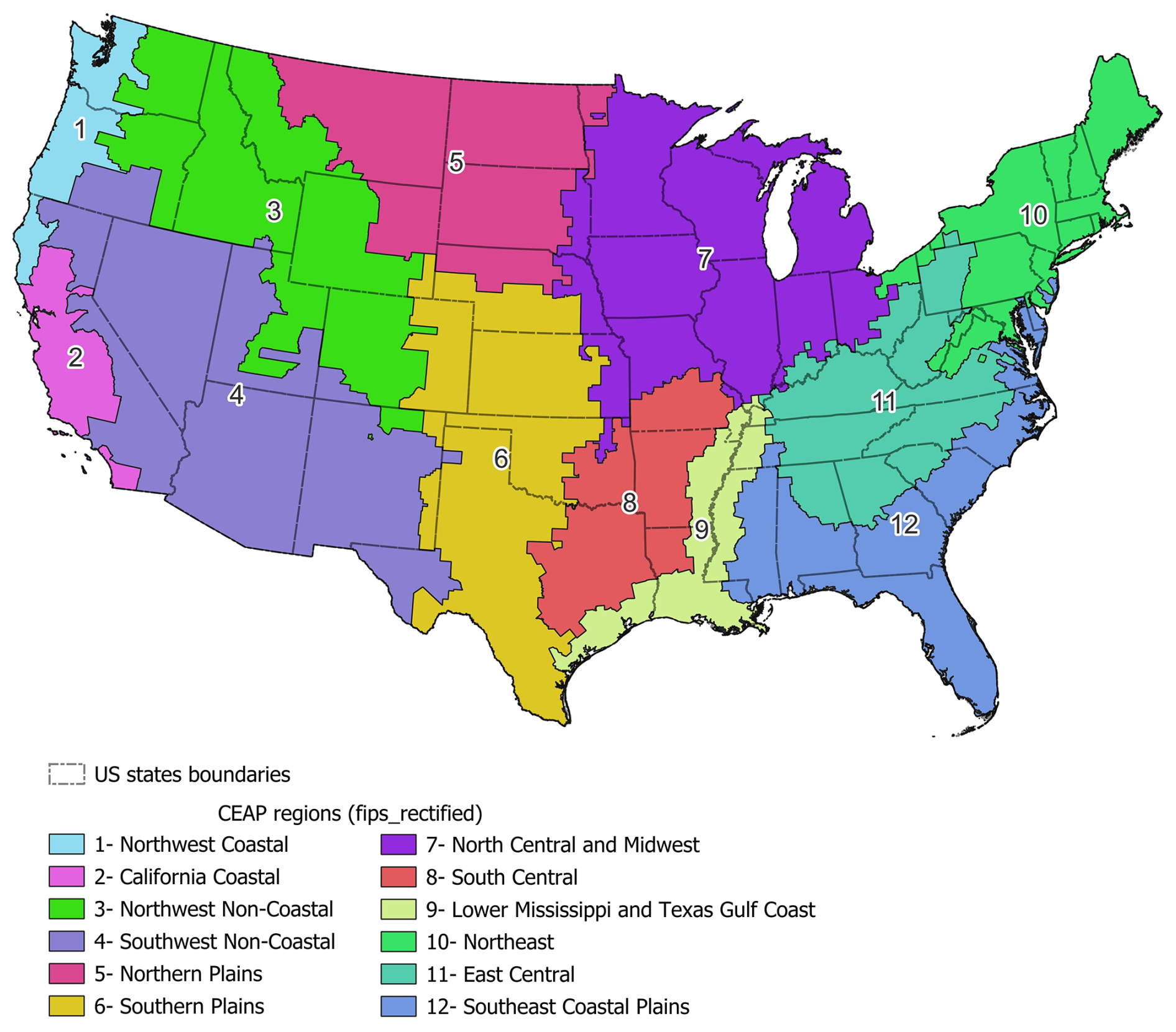
Figure A2Map of 12 CEAP Regions used in analysis as a spatial stratification variable.
Gradient boosted modeling (GBM) (Friedman, 2001) is a machine learning algorithm where multiple weak regression or classification models are combined to optimize predictions. We implemented GBM to predict the season of planting for small grains (wheat, barley, and oats), state-level average synthetic N fertilizer and manure amendment rates, and the survey location-level fertilizer and manure rate residuals. We used a Bernoulli loss function to predict the binary outcome for small grain season of planting and a Gaussian loss function to predict the continuous outcomes. All GBMs were fit using the R package gbm (Ridgeway and Developers, 2024).
We tuned each GBM to select an optimal set of hyperparameters. To do so, we divided the data into training and testing data sets by an 8:2 ratio, respectively. We tuned each model to select an optimal set of hyperparameters such that the loss function was minimized on the testing data set (i.e. minimized validation error). The tuning hyperparameters included the depth of each tree (interaction depth), the learning rate (shrinkage), the minimum number of observations in a terminal node, and the sub-sampling rate (bag fraction). We considered interaction depths of 10 and 15, learning rates of 0.01, 0.1, and 0.2, minimum terminal node observations of 10 and 15, and bag fractions of 0.8 and 1. All possible combinations of tuning parameters were considered to create 24 candidates sets of parameters. For each candidate set, we ran the GBM for 3000 iterations and selected the iteration with the smallest validation error as the best iteration for that candidate set. Then, the candidate set with the smallest validation error on its best iteration was selected as the final set of tuned hyperparameters.
Upon fitting the final GBM, we used the tuned hyperparameters and a train fraction of 1. We used the fitted GBM to predict on the prediction data set, which was either the NRI sample or a state-crop-year grid.
We used Markov transition models when imputing a categorical management activity with high location-level temporal correlation, such as tillage system types (NT, RT, FT) and cover crop adoption (yes/no). The Markov transition model consists of first imputing the management activity for a starting time step (e.g. the 2020–2025 time block for tillage or the year 2023 for cover crops) and then constructing a transition matrix that contains the probability of transitioning to a new category in the subsequent time step (i.e. previous year block or previous year). In our analyses, the transition probabilities were calculated based on linear model predictions of the proportions of tillage system types or cover crop adoption. To describe a general case, let n denote the number of categories for a specific management activity. The transition matrix is an n×n matrix M created from vectors a and b, where a is a vector of n probabilities for the current time step and b is a vector of n probabilities for the subsequent time step. The matrix M is constrained such that: (1) the columns of M are probability distributions, (2) the diagonal elements of M are as large as possible, and (3) Ma=b. We solved the matrix M using linear programming in the R package lpsolve (Berkelaar, 2024). The constraints ensure the highest possible location-level temporal correlation given the probabilities for each category at each time step.
The NRI sample imputations were informed by multiple data sets and computed using a variety of statistical techniques. We evaluated the statistical imputation techniques and compared the imputed values to the observed data.
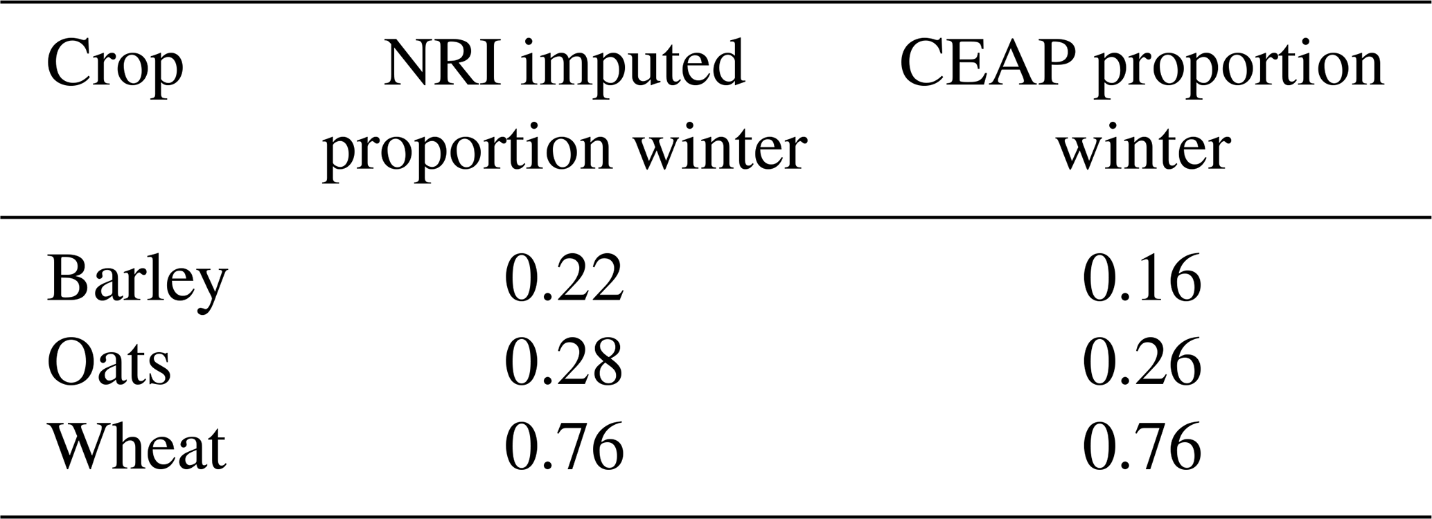
The season of planting for small grains (wheat, barley, and oats) was unknown in the NRI sample, so we predicted the season using a gradient boosted classification model (GBM) trained on the CEAP data. We evaluated the GBM by its training and validation error and relative influence plots. The training error was 0.16 and the validation error was 0.27, which is a relative difference of 66.17 %, suggesting some over-fitting. Major Land Resource Area (MLRA) was the most influential predictor, followed by crop, then longitude and latitude (Table D1). We also calculated the proportion of winter grains imputed on the NRI sample and the proportion of winter grains in the CEAP data (Table D2). The proportion of winter wheat and oats observed in the CEAP data closely matched the proportions imputed on the NRI sample. The proportion of winter oats imputed on the NRI sample was 27 % higher than that observed in CEAP, which may be due to over-fitting of the GBM and limited data available in CEAP to inform planting season for oats.
Table D1Relative influence of each variable in GBM for imputing small grain season of planting.
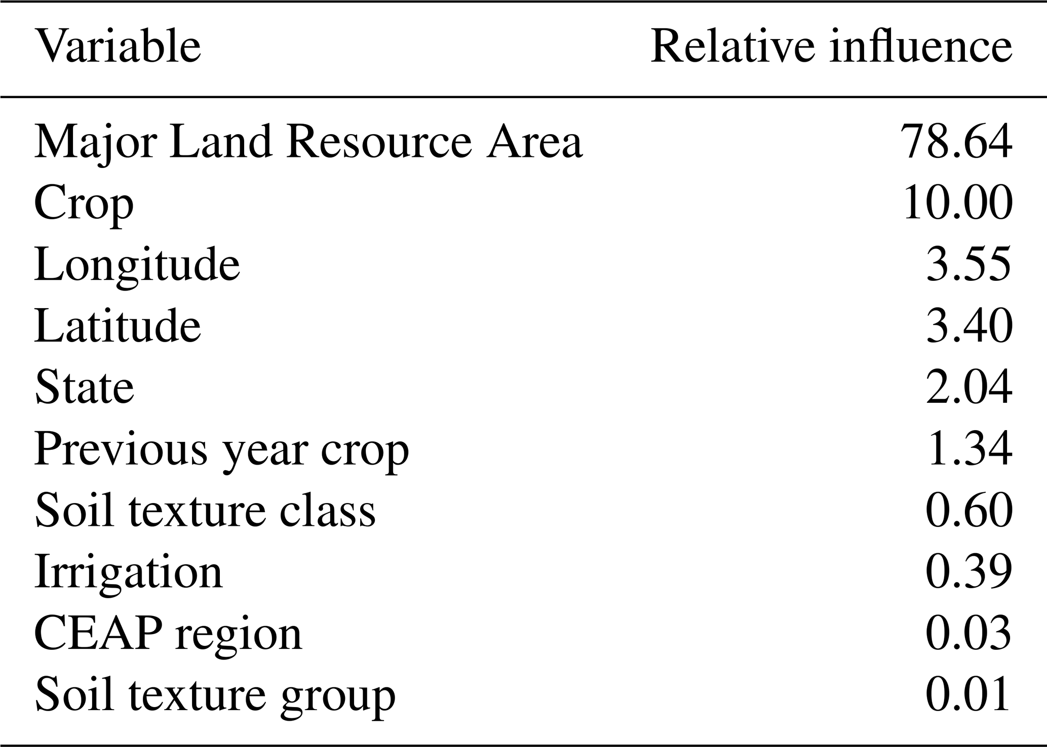
Table D2Proportions of small grains planted in winter that were imputed on the NRI sample and observed in CEAP data sets.
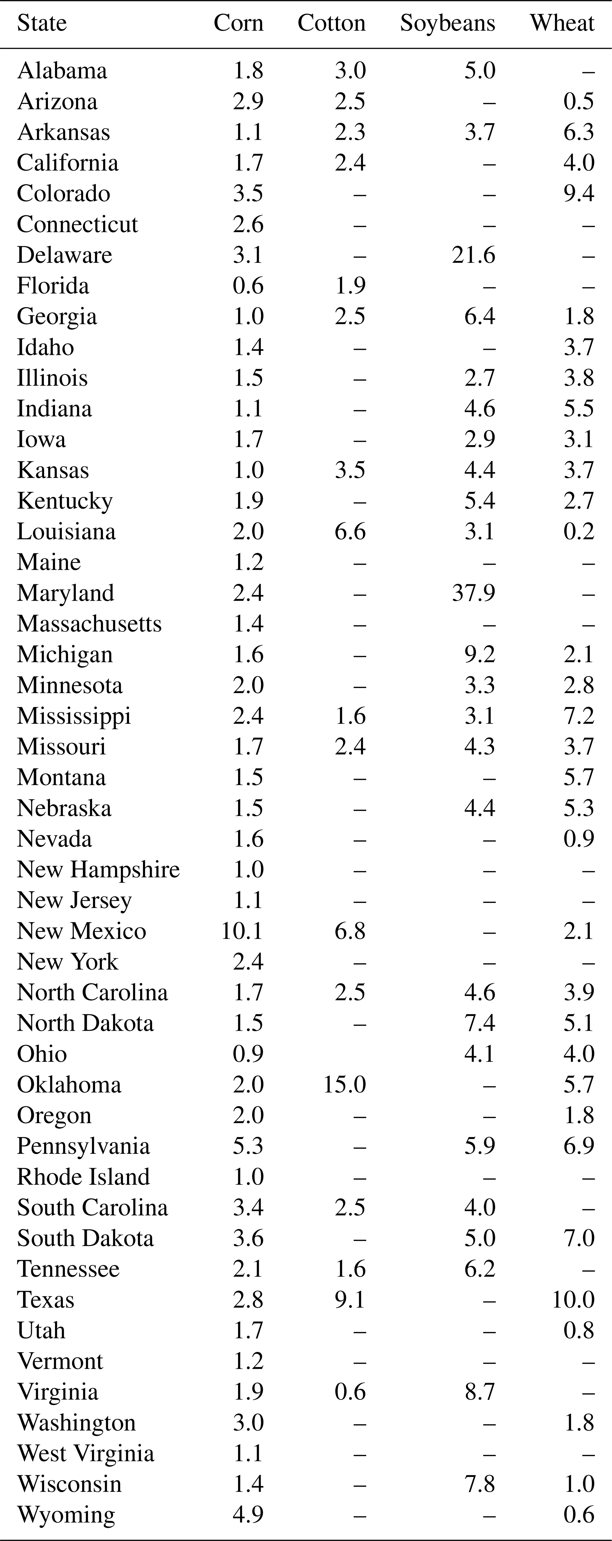
We evaluated synthetic N fertilizer rate imputations in several ways. First, we evaluated the GBM for predicting the percent of cropland area fertilized via the training and validation error and relative influence plots. The training error for percent cropland area fertilized was 15.79 and the validation error was 48.48. The substantially higher validation error suggests possible over-fitting and lack of generalization of the model. Crop was the most influential predictor, followed by state and year (Table D3). Second, we calculated RMSE for the observed vs. predicted percent of cropland area fertilized for each state and crop (Table D4). RMSE was less than 10 percentage points for most state-crop combinations, with some exceptions. Specifically, RMSE was greater than 10 for predictions of cropland area fertilized for soybeans in Maryland (RMSE = 37.9) and Delaware (RMSE = 21.6), cotton in Oklahoma (RMSE = 15.0), and corn in New Mexico (RMSE = 10.1). For these state-crop combinations, few observations informed the predictions, and the available data tended to differ substantially from data for similar crops and states. Furthermore, the percent of cropland area in these states is a relatively small proportion of the total cropland area in CONUS (<2.5 %).
Table D3Relative influence of each variable in the GBM for predicting percent of cropland area applying synthetic N fertilizer.
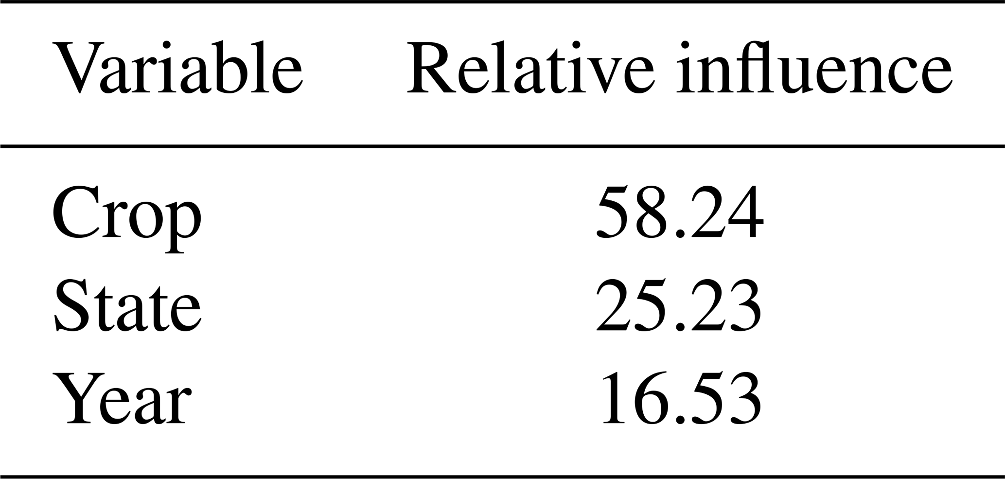
Table D4Root mean squared error for observed vs. predicted percent of cropland area fertilized by state and crop. Blank values indicate a lack of data for the state and crop.
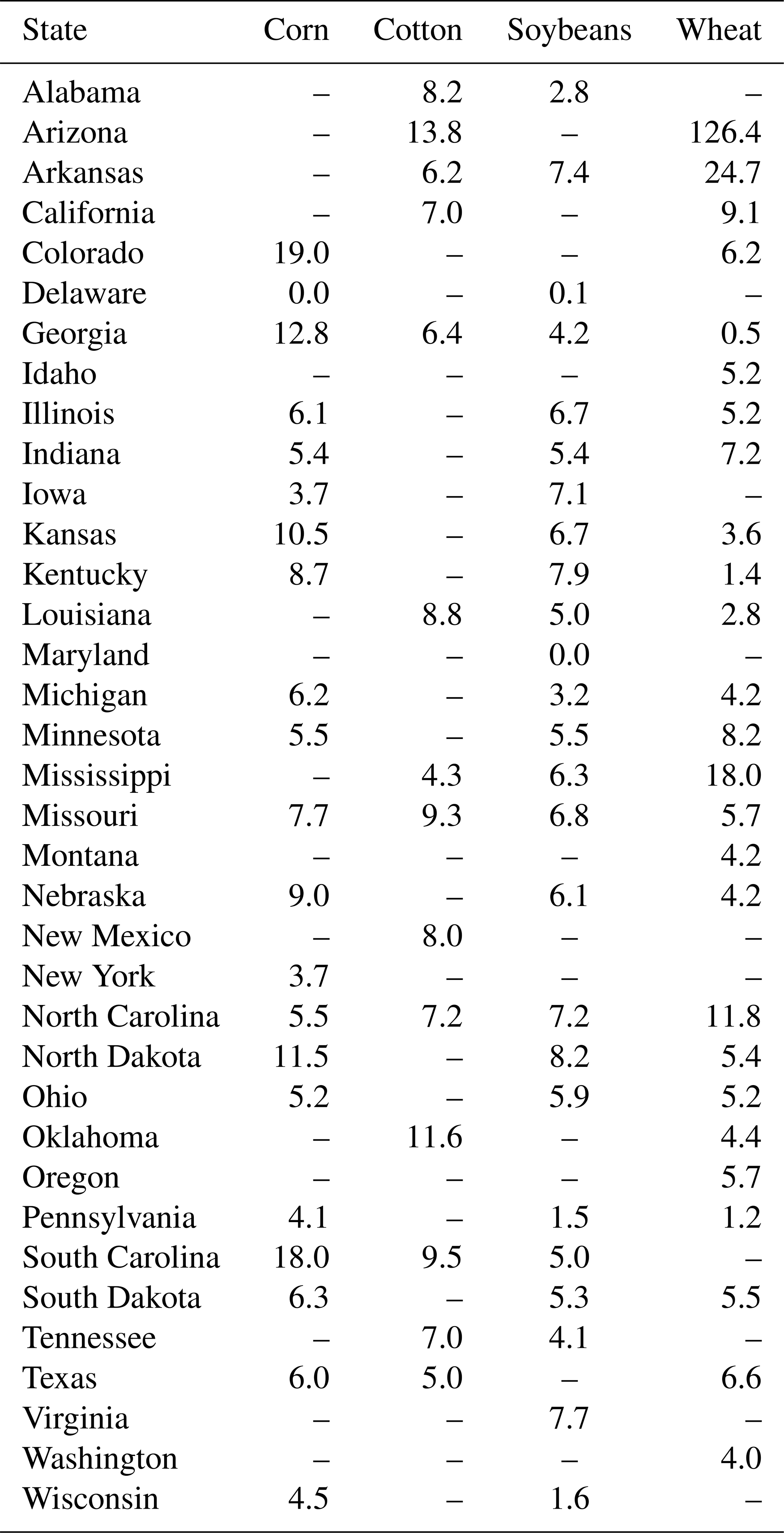
Next we evaluated the GBM for predicting state-level average synthetic N fertilization rates. The training error was 31.49 and the validation error was 160.08. Crop was the most influential predictor, followed by year and state (Table D5). The difference between training and validation errors suggests the GBM did not generalize to state-crop-year combinations outside the range of the data. We calculated RMSE for the predicted vs. observed state-level average annual synthetic N fertilization rates for each crop (Table D6). RMSE was less than 20 kg ha−1 for most combinations of states and crops. State-crops with higher RMSE were those with limited data available (e.g. often 3 or fewer observed data values). Hence, predictions matched the data for state-crops that had a reasonable amount of data available.
Table D5Relative influence of predictor variables in GBM for predicting state-level annual average fertilization rates.
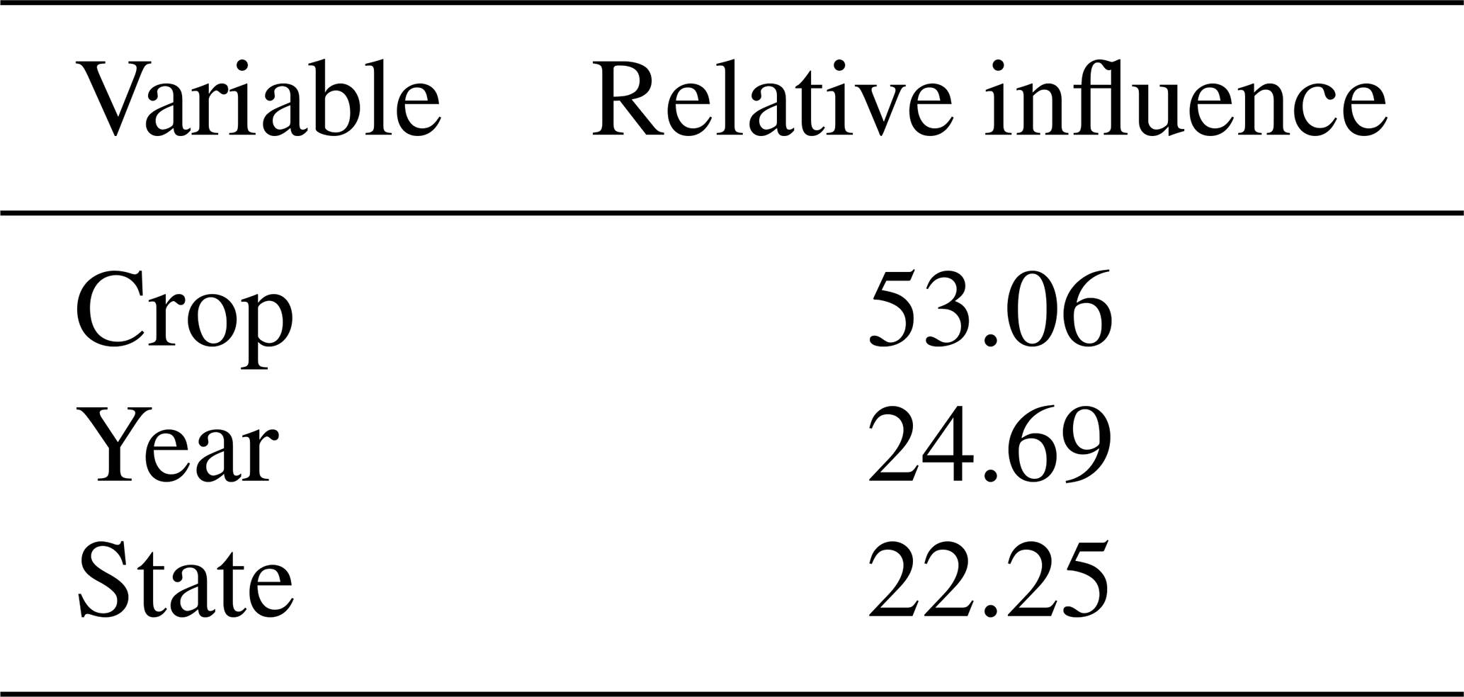
Table D6Root mean squared error for predicted vs. observed state-level annual average synthetic N fertilization rates by state and crop. Blank values indicate a lack of data for the state and crop.
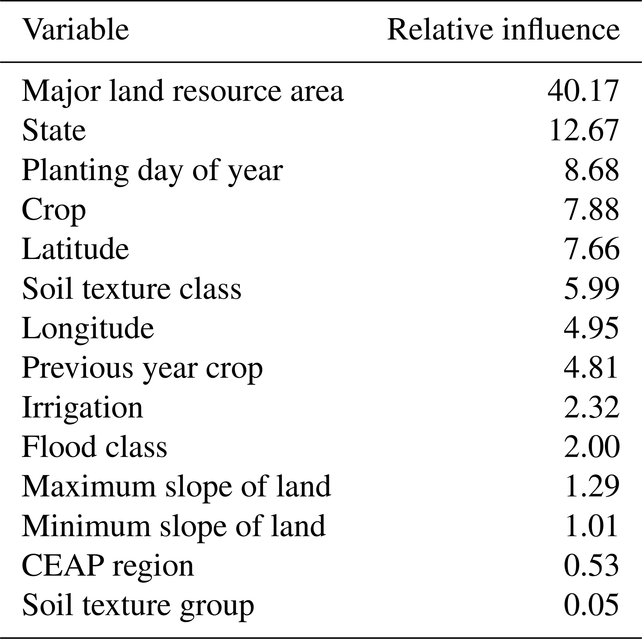
Finally, we evaluated the GBM for predicting the residual difference between location-level fertilization rates in CEAP and the predicted state-crop-year average fertilization rates. The training error was 3026.58 and the validation error was 3567.63, a 15.17 % difference. Note that errors are on the squared scale; hence, these validation errors correspond to scaled errors of 54 to 59 kg N ha−1. MLRA was the most influential predictor, followed by state, planting day of year, crop, latitude, soil texture class, longitude, and previous crop (Table D7). RMSE for the imputed fertilizer rates vs. observed values in CEAP across all states and crops was 69.3 kg N ha−1 yr−1.
Table D7Relative influence of predictor variables in GBM for predicting the residual difference in fertilization rates from state-level averages.
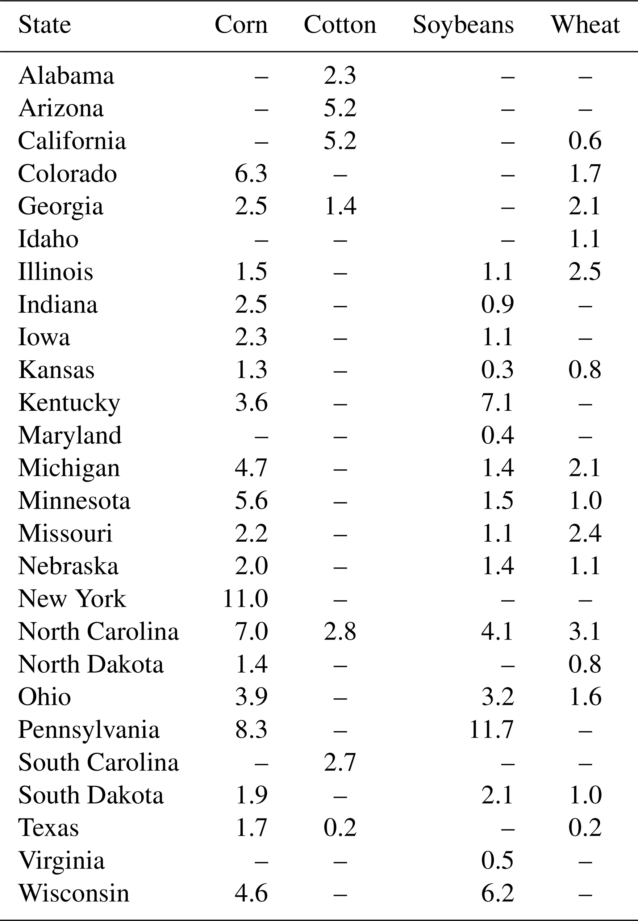
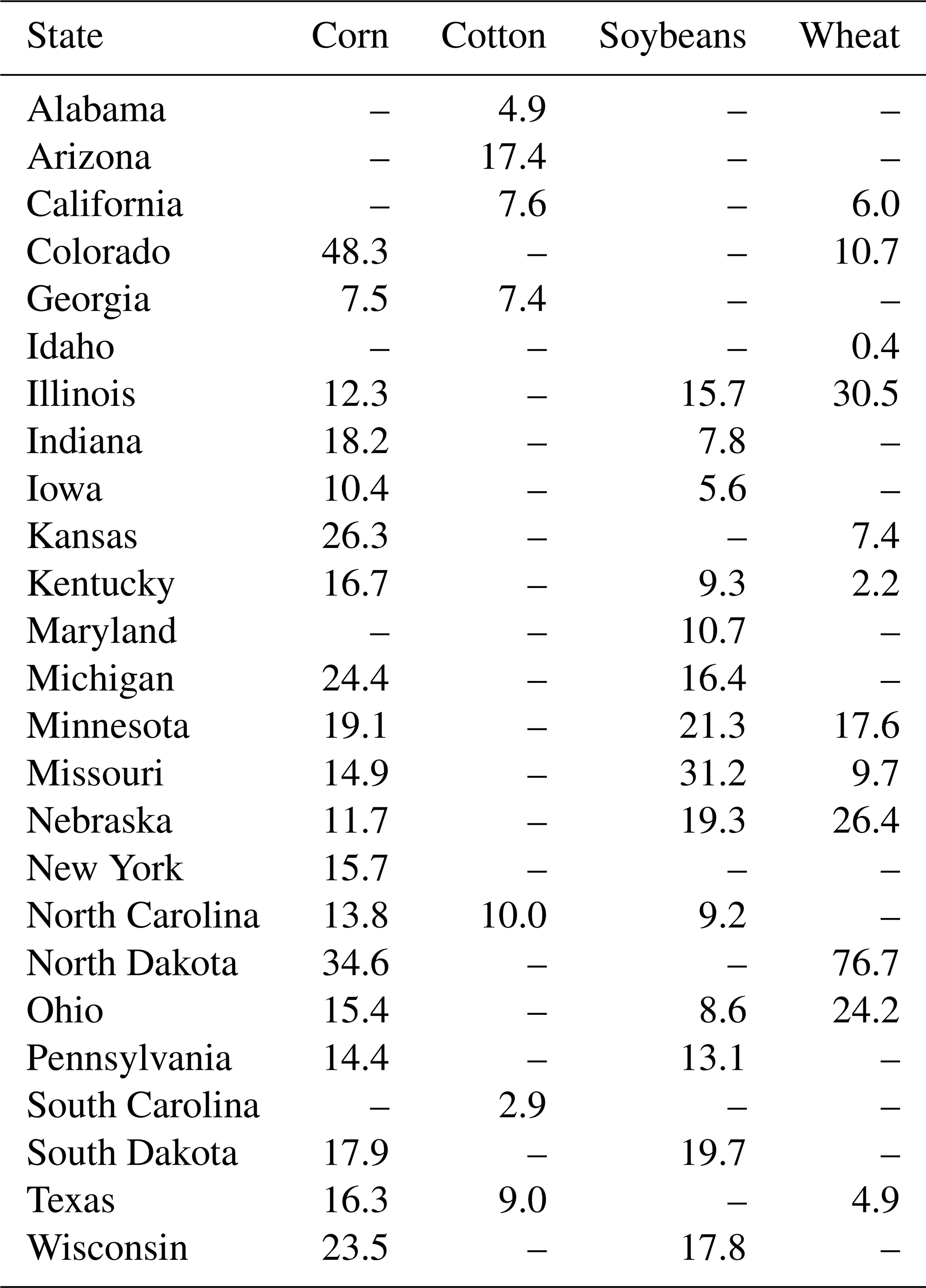
We similarly evaluated manure N amendment rate imputations. For the GBM predicting state-level percent cropland area with manure amendments, the training error was 49.07 and the validation error was 45.79. Year was the most influential predictor, followed by state and crop (Table D8). We calculated RMSE for the observed vs. predicted percent of cropland area with manure amendments for each state and crop (Table D9). Manure amendment data was only available for the 26 states listed in the table. RMSE was below 10 percentage points for all state-crop combinations except for corn in New York and soybeans in Pennsylvania. These state-crop combinations had little data to inform them and represent a small proportion of the total cropland area in CONUS.
Table D8Relative influence of each variable in the GBM for predicting percent of cropland area applying manure amendments.
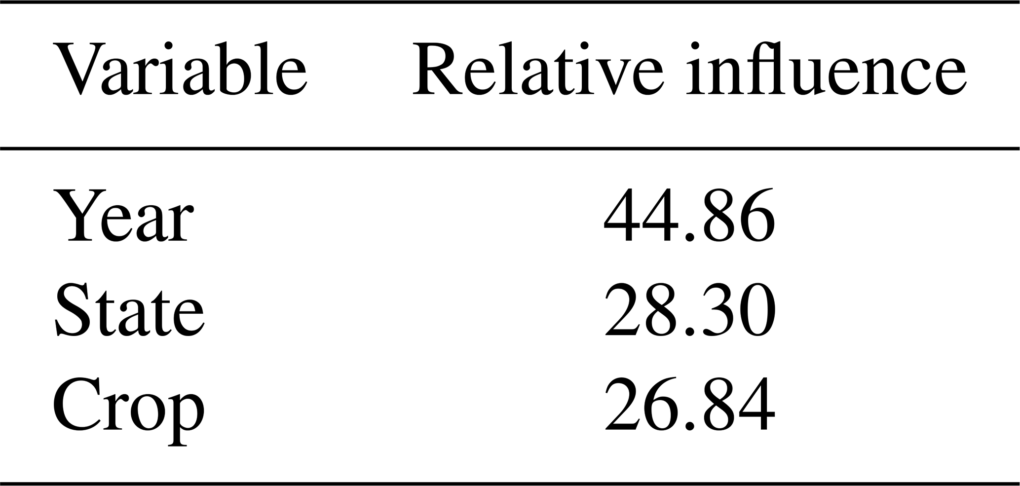
Table D9Root mean squared error observed vs. predicted percent of cropland area using manure amendments by state and crop. Blank values indicate a lack of data for the state and crop. States not listed lacked data on manure amendments.
In the GBM for predicting state-level manure N rates, the training error was 421.56 and the validation error was 976.70, suggesting a high level of uncertainty in the predicted state-level rates. The most influential predictor variable was state, followed by year, crop, and relative N available (Table D10). We calculated RMSE for the predicted vs. observed state-level average annual manure N rates for each crop (Table D11). RMSE was greater than 20 kg ha−1 for 11 out of 52 state-crop combinations. This is likely due to limited data informing rates in many state-crop combinations.
Table D10Relative influence of predictor variables in GBM for predicting state-level annual average manure N rates.
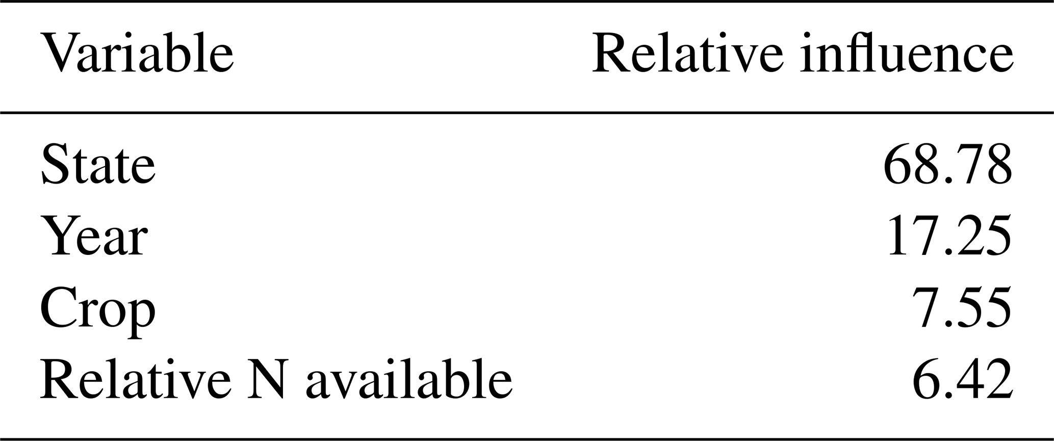
Table D11Root mean squared error for predicted vs. observed state-level annual average manure N rates by state and crop. Blank values indicate a lack of data for the state and crop. States not listed lacked data on manure amendments.
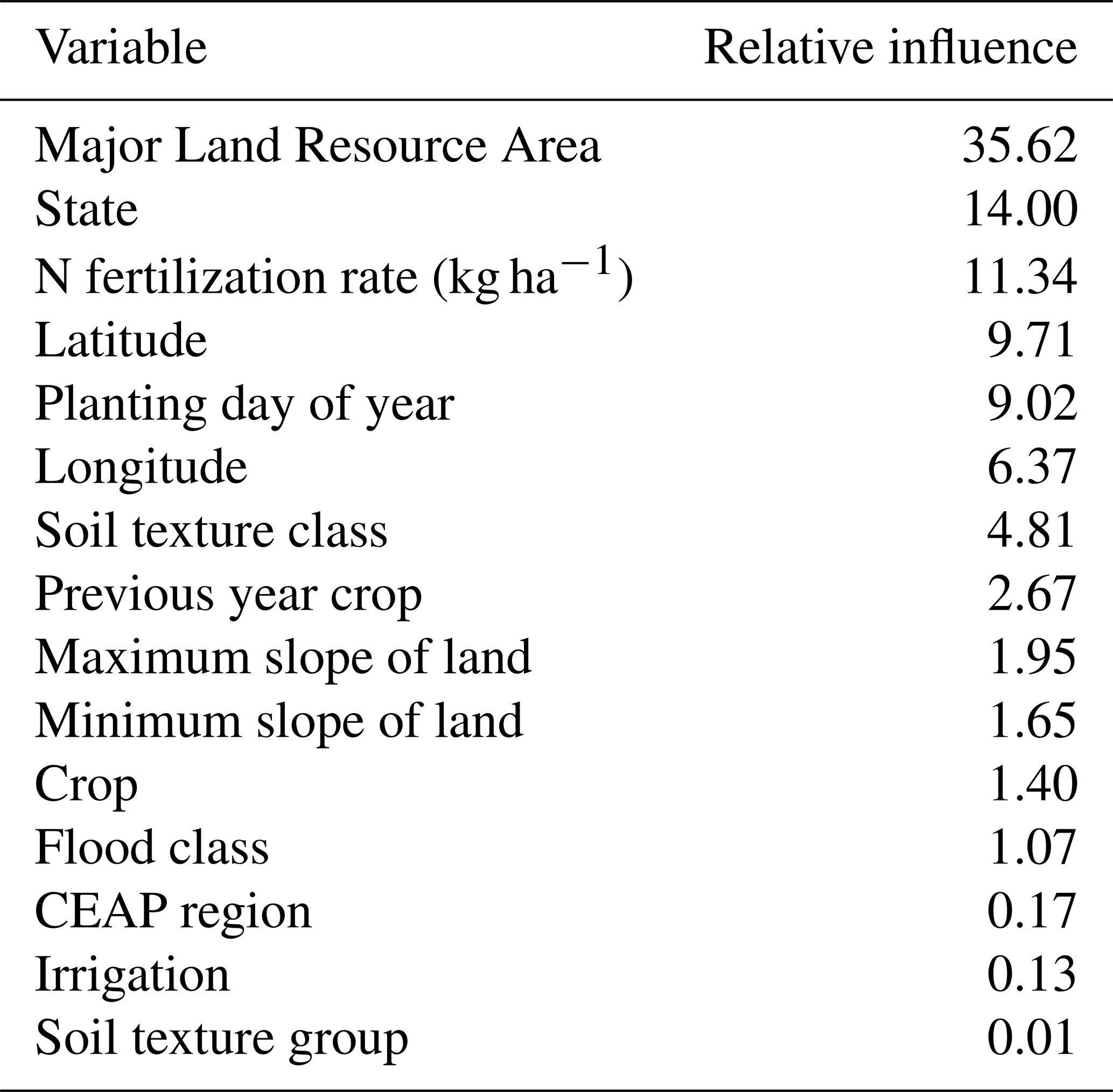
Regarding the GBM used to predict residual differences between location-level manure N rates in CEAP and the predicted state-level average rates, the training error was 7131.07 and the validation error was 8265.61. The GBM demonstrated similar performance on in-sample vs. out-of-sample predictions and had scaled error rates of approximately 84 to 90 kg N ha−1. MLRA was the most influential predictor, followed by state, synthetic N fertilization rate, latitude, planting date, longitude, soil texture class, and previous year crop (Table D12). RMSE for the imputed manure rates vs. observed values in CEAP across all states and crops was 122.0 kg N ha−1 yr−1.
Table D12Relative influence of predictor variables in GBM for predicting the residual difference in manure N rates from state-level averages.
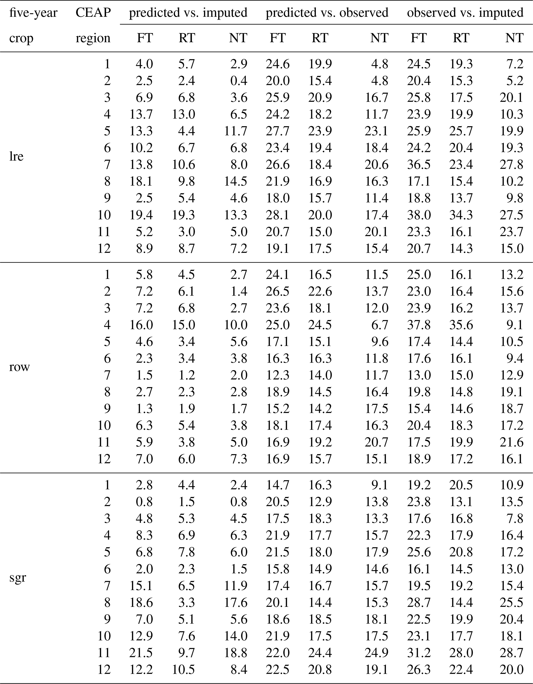
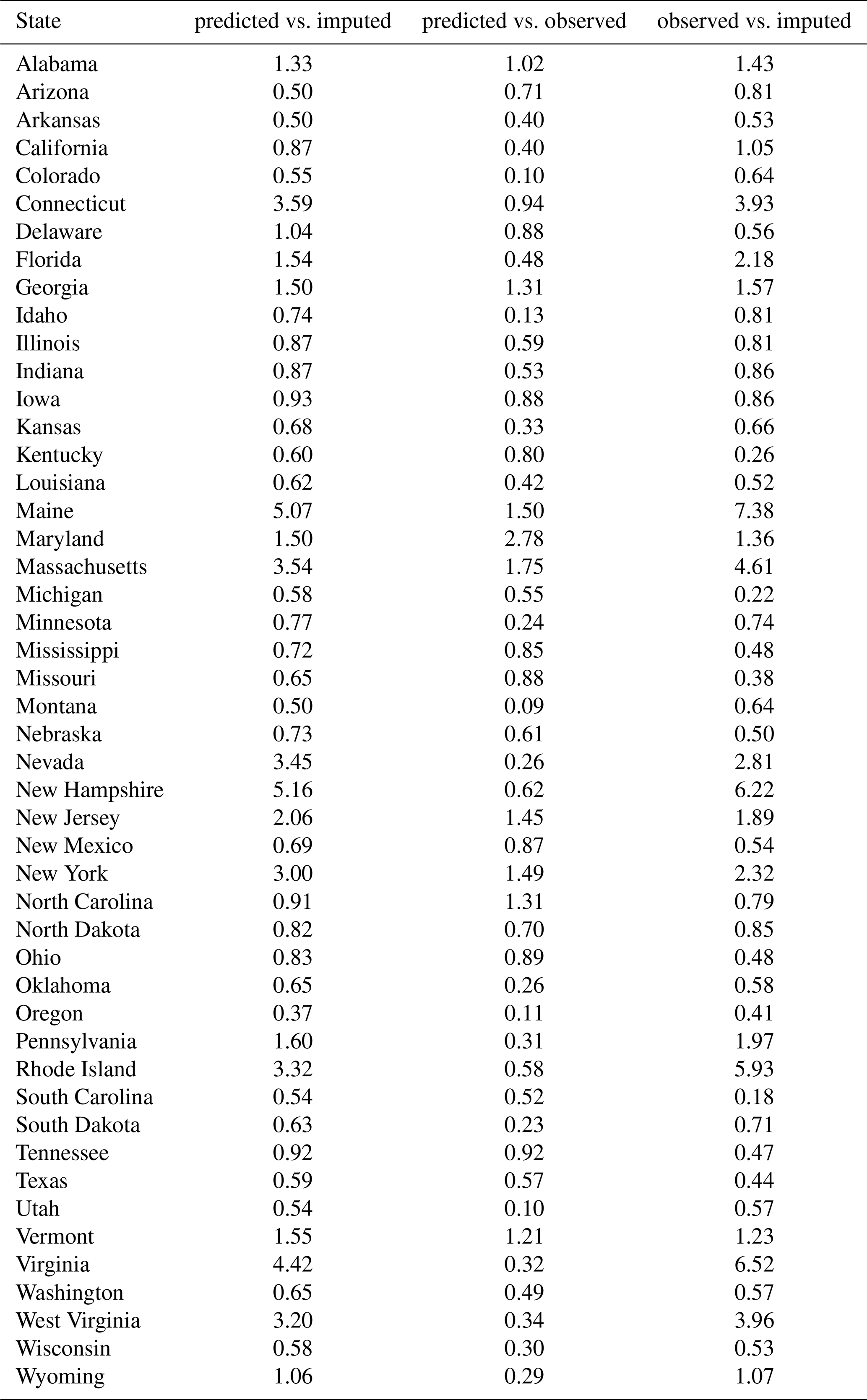
To evaluate tillage system imputations, we compared the NRI sample imputations to the observed data and the predictions from the linear models. We calculated RMSE for the predicted vs. imputed, predicted vs. observed, and observed vs. imputed percent of tillage system types by crop group (low residue (lre), row crops (row), and small grains (sgr)) and CEAP region to evaluate both the linear model predictions and Markov transition imputations for tillage system types (Table D13). The observed data are aggregated data from OpTIS and CEAP. The RMSE for predicted vs. imputed tillage system type percentages was generally relatively small, and consistently smaller than that for predicted vs. observed and observed vs. imputed percentages. Hence, the Markov transition model generated imputations that matched the predicted output from the linear models. However, the combination of multiple data sources and high variability over time and across space created a noisy data set for the linear model, leading to high RMSE for predicted vs. observed percents. This variability carried over into the RMSE for observed vs. imputed values.
Table D13Root mean squared error (RMSE) for the percent of each tillage system type by crop group (sgr = small grains, row = row crops, lre = low residue crops). RMSE was calculated for linear model predictions (predicted) vs. NRI sample imputations (imputed), predicted vs. observed data values (from CEAP and OpTIS), and observed vs. imputed values.
To evaluate cover crop imputations, we similarly calculated RMSE for the predicted vs. imputed, predicted vs. observed, and observed vs. imputed percent of cropland area using cover crops by state. RMSE for imputed vs. observed cover crop percentage was less than 7.5 percentage points in all states, showing that the imputation approach closely matched the observed values. RMSE for predicted vs. observed and predicted vs. imputed was even smaller, suggesting the patterns captured by the linear model were maintained in the Markov transition model when imputing on the NRI survey locations.
Table D14Root mean squared error (RMSE) for percent of cropland area with cover crop adoption in each state. RMSE was calculated for linear model predictions (predicted) vs. NRI sample imputations (imputed), predicted values vs. observed data values (from US Agricultural Census), and observed values vs. imputed values.
The imputed percent of cover crop adoption for the cropland area in our analyses increased over time in all CEAP regions (Table E1). Some CEAP region were quicker to adopt cover crops, particularly the Northeast, East Central, and Southeast Coastal Plains. These regions had over 10 % cropland area with cover crops by 2020. Other regions were slower to adopt cover crops, namely, the Northern and Southern Plains and Northwest and Southwest Non-Coastal regions, likely due to the long winters and arid climate.
The proportion of tillage system types for low residue crops (cotton) and small grains (wheat, barley, and oats) for 1980, 2000, and 2020 are shown in Figs. E1 and E2, respectively. For both crop groups, the proportion of cropland area managed with NT and RT tillage systems generally increased over time, while the proportion managed with FT tillage systems decreased. The western regions experienced the least shift over time, with most cropland area still managed with FT systems by 2020. The middle latitudes experienced a moderate shift towards NT and RT systems, and the eastern regions experienced the most rapid shift towards NT and RT systems. By 2020, NT systems were the most common tillage system type in the northern Central Plains and Midwest for small grains and in the Southeast for low residue crops.
Table E1Percent of cropland area with cover crop adoption each decade from 1990–2020 by CEAP region.
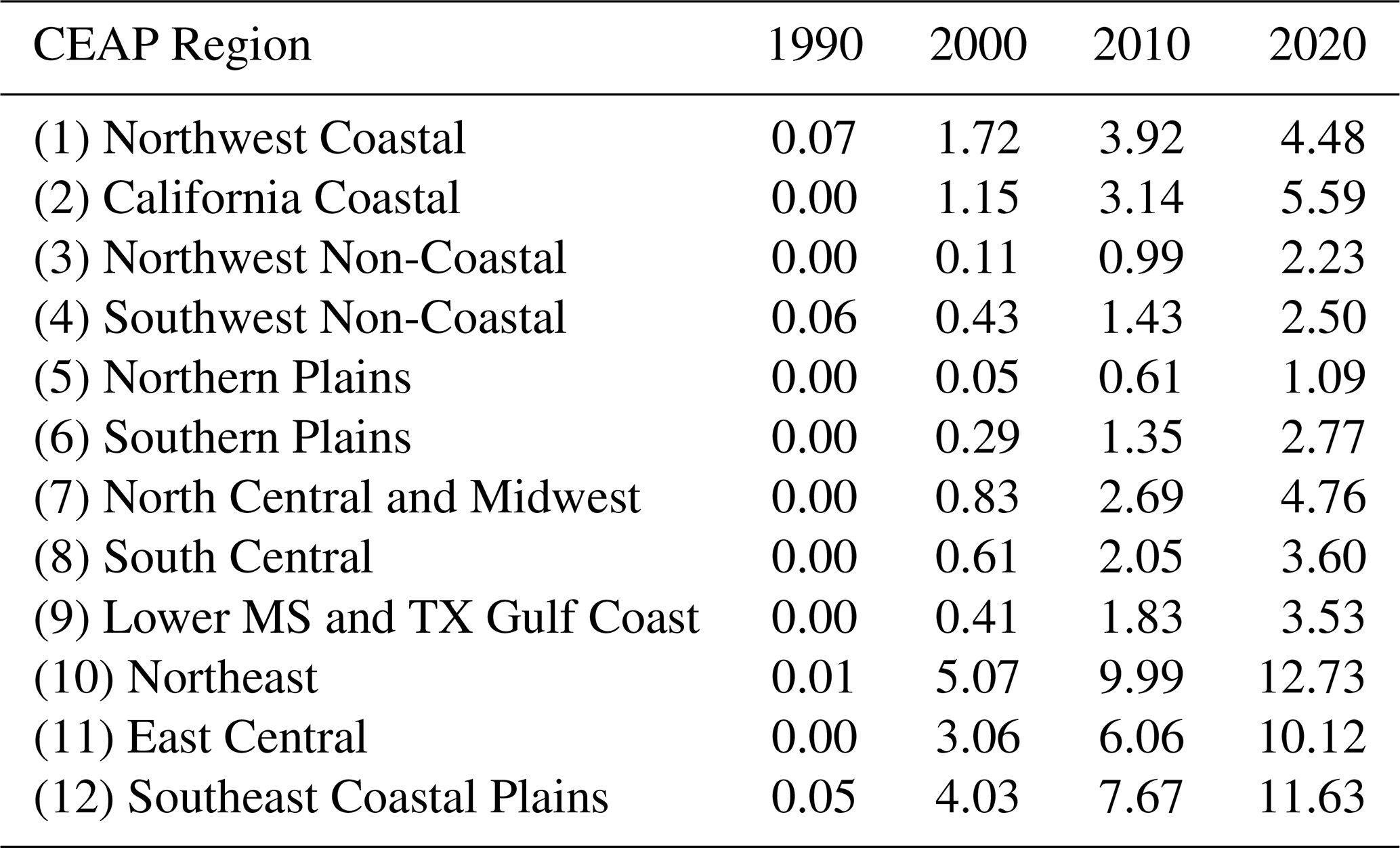
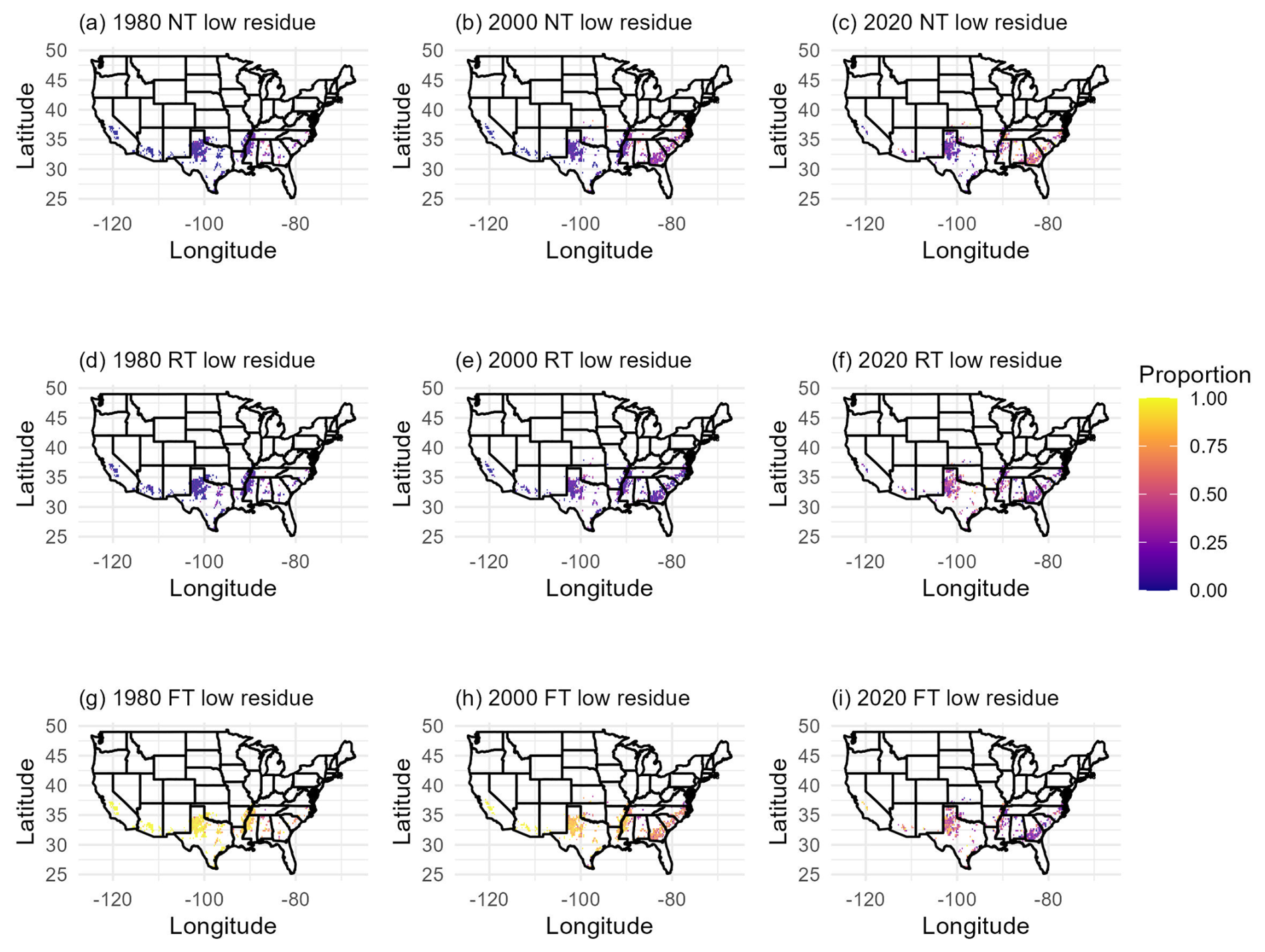
Figure E1Proportion of low residue crop (cotton) cropland area managed with each tillage system type (FT = full/conventional tillage, RT = reduced tillage, NT = no tillage) across CONUS for 1980, 2000, and 2020.
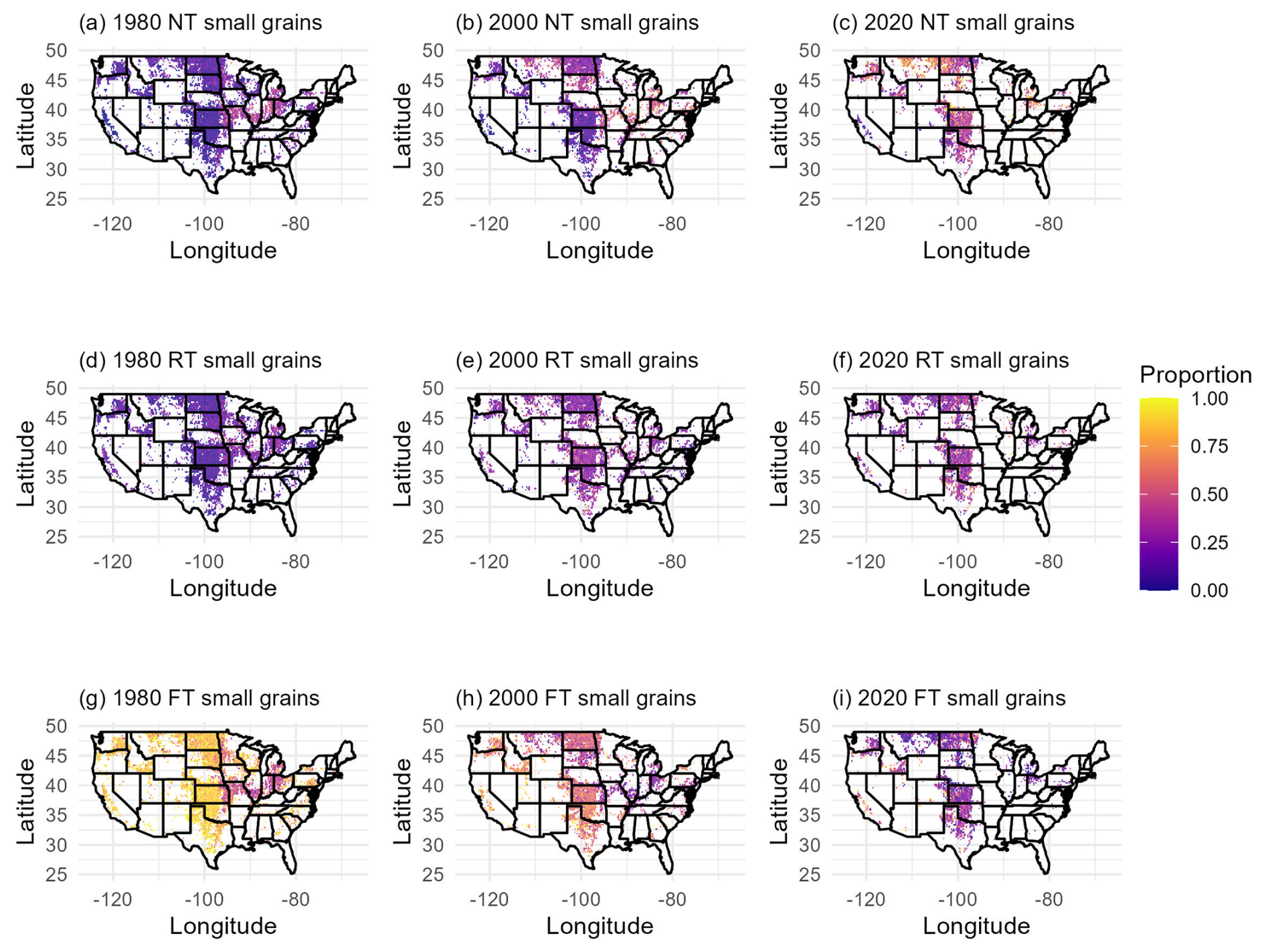
Figure E2Proportion of small grain (wheat, barley, and oats) cropland area managed with each tillage system type (FT = full/conventional tillage, RT = reduced tillage, NT = no tillage) across CONUS for 1980, 2000, and 2020.
Lauren Hoskovec developed methodology, conducted formal analyses, developed software and code to implement algorithms, and prepared the original manuscript draft. Stephen Ogle acquired funding, supervised and managed the project leading to this publication, and reviewed and edited the manuscript drafts. F. Jay Breidt helped develop methodology. Alisa R. Keyser and Shannon L. Spencer assisted with data curation, visualization, and reviewing and editing manuscript drafts. Yesar Ahmed Oshan revised analyses based on reviewer comments. Teng Liu developed software and code to implement algorithms. Stephen Williams helped develop ideas and acquire data to implement analyses.
The contact author has declared that none of the authors has any competing interests.
Publisher's note: Copernicus Publications remains neutral with regard to jurisdictional claims made in the text, published maps, institutional affiliations, or any other geographical representation in this paper. The authors bear the ultimate responsibility for providing appropriate place names. Views expressed in the text are those of the authors and do not necessarily reflect the views of the publisher.
We are grateful for funding support from USDA-Office of the Chief Economist (Cooperative Agreements 58-0111-22-016, 58-0111-23-013, and 58-0111-24-025). We acknowledge Cody Alsaker who developed an earlier version of the management data. We also acknowledge Veronica Thompson and Shahriar Shah Heydari who assisted with data cleaning, quality control, and data visualization.
This research has been supported by the U.S. Department of Agriculture (grant nos. 58-0111-22-016, 58-0111-23-013, and 58-0111-24-025).
This paper was edited by Peng Zhu and reviewed by Yushu Xia and one anonymous referee.
AAPFCO: Association of American Plant Food Control Officials Commercial Fertilizers, reports covering the years 1995–2000a, 2002–2007, 1995–2007. a
AAPFCO: Association of American Plant Food Control Officials Commercial Fertilizers: 2008–2017, reports covering the years 2008–2017, 2008–2022. a, b
Adalibieke, W., Cui, X., Cai, H., You, L., and Zhou, F.: Global crop-specific nitrogen fertilization dataset in 1961–2020, Sci. Data, 10, https://doi.org/10.1038/s41597-023-02526-z, 2023. a
Andridge, R. R. and Little, R. J.: A review of hot deck imputation for survey non-response, Int. Stat. Rev., 78, 40–64, https://doi.org/10.1111/j.1751-5823.2010.00103.x, 2010. a
Berkelaar, M.: lpSolve: Interface to “Lp solve” v. 5.5 to Solve Linear Integer Programs, r package version 5.6.23, https://CRAN.R-project.org/package=lpSolve (last access: 6 November 2026), 2024. a
Bian, Z., Tian, H., Yang, Q., Xu, R., Pan, S., and Zhang, B.: Production and application of manure nitrogen and phosphorus in the United States since 1860, Earth Syst. Sci. Data, 13, 515–527, https://doi.org/10.5194/essd-13-515-2021, 2021. a, b, c, d, e
Brakebill, J. and Gronberg, J.: County-Level Estimates of Nitrogen and Phosphorus from Commercial Fertilizer for the Conterminous United States, 1987–2012, U.S. Geological Survey data release [data set], https://doi.org/10.5066/F7H41PKX, 2017. a, b, c
Cao, P., Lu, C., and Yu, Z.: Historical nitrogen fertilizer use in agricultural ecosystems of the contiguous United States during 1850–2015: application rate, timing, and fertilizer types, Earth Syst. Sci. Data, 10, 969–984, https://doi.org/10.5194/essd-10-969-2018, 2018. a, b, c, d, e, f, g
CDL: National Agricultural Statistics Service Cropland Data Layer, https://www.nass.usda.gov/Research_and_Science/Cropland/SARS1a.php (last access: 6 November 2026), 2024. a
CTIC: Conservation Technology Information Center Crop Residue Management Survey, https://www.ctic.org/CRM_NEW (last access: 6 November 2026), 2004. a
Derpsch, R., Friedrich, T., Kassam, A., and Hongwen, L.: Current status of adoption of no-till farming in the world and some of its main benefits, Int. J. Agr. Biol. Eng., 3, 1–25, https://doi.org/10.3965/j.issn.1934-6344.2010.01.001-025, 2010. a
EPA: Inventory of U.S. Greenhouse Gas Emissions and Sinks: 1990–2022, https://www.epa.gov/ghgemissions/inventory-us-greenhouse-gas-emissions-and-sinks-1990-2022 (last access: 6 November 2026), 2024. a, b, c, d, e, f
Falcone, J. A.: Estimates of county-level nitrogen and phosphorus from fertilizer and manure from 1950 through 2017 in the conterminous United States, Open-File Report 2020–1153, U.S. Geological Survey, ISSN 2331-1258, https://doi.org/10.3133/ofr20201153, 2021. a
Fancher, H., Nagler, A., Ritten, J., and Wulfhorst, J. D.: US Beef Cattle Inventory Trends With Implications for Land Use and Rangelands, Rangeland Ecol. Manag., 103, 545–553, https://doi.org/10.1016/j.rama.2025.01.007, 2025. a
Farooq, M. and Siddique, K. H.: Conservation agriculture: Concepts, brief history, and impacts on agricultural systems, in: Conservation Agriculture, Springer International Publishing, 3–17, ISBN 9783319116204, https://doi.org/10.1007/978-3-319-11620-4_1, 2015. a
Friedman, J. H.: Greedy Function Approximation: A Gradient Boosting Machine, Ann. Stat., 29, 1189–1232, 2001. a
Gurung, R. B., Ogle, S. M., Breidt, F. J., Williams, S. A., and Parton, W. J.: Bayesian calibration of the DayCent ecosystem model to simulate soil organic carbon dynamics and reduce model uncertainty, Geoderma, 376, https://doi.org/10.1016/j.geoderma.2020.114529, 2020. a
Hagen, S. C., Delgado, G., Ingraham, P., Cooke, I., Emery, R., Fisk, J. P., Melendy, L., Olson, T., Patti, S., Rubin, N., Ziniti, B., Chen, H., Salas, W., Elias, P., and Gustafson, D.: Mapping conservation management practices and outcomes in the corn belt using the operational tillage information system (Optis) and the denitrification–decomposition (DNDC) model, Land, 9, 1–23, https://doi.org/10.3390/land9110408, 2020. a
Hoskovec, L.: aglandmgmt: v1.0.0, Zenodo [data set], https://doi.org/10.5281/zenodo.23987242, 2026. a, b
Hoskovec, L., Ogle, S., Keyser, A., and Spencer, S.: Agricultural land management activities for conterminous US from 1980–2023, Dryad [data set], https://doi.org/10.5061/dryad.t1g1jwtgm, 2026. a, b
IPCC: 2006 IPCC Guidelines for National Greenhouse Gas Inventories, Institute for Global Environmental Strategies (IGES), Hayama, Japan, https://www.ipcc-nggip.iges.or.jp/public/2006gl/index.html (last access: 6 November 2026), 2006. a
IPCC: 2019 Refinement to the 2006 IPCC Guidelines for National Greenhouse Gas Inventories, IPCC, Geneva, Switzerland, https://www.ipcc-nggip.iges.or.jp/public/2019rf/index.html (last access: 6 November 2026), 2019. a
Lombardozzi, D. L., Lu, Y., Lawrence, P. J., Lawrence, D. M., Swenson, S., Oleson, K. W., Wieder, W. R., and Ainsworth, E. A.: Simulating Agriculture in the Community Land Model Version 5, J. Geophys. Res.-Biogeo., 125, https://doi.org/10.1029/2019JG005529, 2020. a, b
Lu, C., Yu, Z., Hennessy, D. A., Feng, H., Tian, H., and Hui, D.: Emerging weed resistance increases tillage intensity and greenhouse gas emissions in the US corn–soybean cropping system, Nature Food, 3, 266–274, https://doi.org/10.1038/s43016-022-00488-w, 2022a. a, b
Lu, C., Yu, Z., Zhang, J., Cao, P., Tian, H., and Nevison, C.: Century-long changes and drivers of soil nitrous oxide (N2O) emissions across the contiguous United States, Glob. Change Biol., 28, 2505–2524, https://doi.org/10.1111/gcb.16061, 2022b. a, b, c
MacDonald, J. M.: Tracking the Consolidation of U.S. Agriculture, Appl. Econ. Perspect. P., 42, 361–379, https://doi.org/10.1002/aepp.13056, 2020. a
Mehring, A., Wallace, H., and Drain, M.: Consumption and Trends in the Use of Fertilizer in the Year Ended June 30, 1944, Tech. rep., United States Department of Agriculture, Washington, D.C., 1946. a
NASS: 1982 National Agricultural Statistics Service Census of Agriculture, https://www.nass.usda.gov/AgCensus/archive/census_year/1982-census/index.html (last access: 6 November 2026), 1982. a
NASS: 1987 National Agricultural Statistics Service Census of Agriculture, https://www.nass.usda.gov/AgCensus/archive/census_year/1987-census/index.html (last access: 6 November 2026), 1987. a
NASS: 2012 National Agricultural Statistics Service Census of Agriculture, https://www.nass.usda.gov/AgCensus/archive/census_year/2012-census/index.html (last access: 6 November 2026), 2012. a
NASS: 2017 National Agricultural Statistics Service Census of Agriculture, https://www.nass.usda.gov/Publications/AgCensus/2017/index.php (last access: 6 November 2026), 2017. a
NASS: 2022 National Agricultural Statistics Service Census of Agriculture, https://www.nass.usda.gov/Publications/AgCensus/2022/index.php (last access: 6 November 2026), 2022. a
Njuki, E.: Sources, Trends, and Drivers of U.S. Dairy Productivity and Efficiency, https://www.ers.usda.gov (last access: 6 November 2026), 2022. a
NRCS: Assessment of the Effects of Conservation Practices on Cultivated Cropland in the Upper Mississippi River Basin, https://www.nrcs.usda.gov/ceap/croplands (last access: 6 November 2026), 2012. a, b, c
NRCS: Conservation Practice on Cultivated Croplands: A Comparison of CEAP 1 and CEAP 2 Survey Data and Modeling, https://www.nrcs.usda.gov/sites/default/files/2022-09/CEAP-Croplands-ConservationPracticesonCultivatedCroplands-Report-March2022.pdf (last access: 6 November 2026), 2022. a, b, c
Nusser, S. and Goebel, J.: The National Resources Inventory: a long-term multi-resource monitoring programme, Environ. Ecol. Stat., 4, 181–204, 1997. a
Ogle, S. M., Alsaker, C., Baldock, J., Bernoux, M., Breidt, F. J., McConkey, B., Regina, K., and Vazquez-Amabile, G. G.: Climate and Soil Characteristics Determine Where No-Till Management Can Store Carbon in Soils and Mitigate Greenhouse Gas Emissions, Sci. Rep., 9, https://doi.org/10.1038/s41598-019-47861-7, 2019. a
Ogle, S. M., Breidt, F. J., Del Grosso, S., Gurung, R., Marx, E., Spencer, S., Williams, S., and Manning, D.: Counterfactual scenarios reveal historical impact of cropland management on soil organic carbon stocks in the United States, Sci. Rep., 13, https://doi.org/10.1038/s41598-023-41307-x, 2023. a
Ogle, S. M., Adler, P. R., Bentrup, G., Derner, J., Domke, G., Del Grosso, S., Lehmann, J., Reba, M., and Woolf, D.: Chapter 3: Quantifying greenhouse gas sources and sinks in cropland and grazing land systems, in: Quantifying Greenhouse Gas Fluxes in Agriculture and Forestry: Methods for Entity‐Scale Inventory, edited by: Hanson, W. L., Itle, C., and Edquist, K., Technical Bulletin Number 1939, U.S. Department of Agriculture, Office of the Chief Economist, Washington, DC, 2nd Edn., https://research.fs.usda.gov/treesearch/67709 (last access: 9 November 2026), 2024. a, b
Paustian, K., Lehmann, J., Ogle, S., Reay, D., Robertson, G. P., and Smith, P.: Climate-smart soils, Nature, 532, 49–57, https://doi.org/10.1038/nature17174, 2016. a
Porwollik, V., Rolinski, S., Heinke, J., and Müller, C.: Generating a rule-based global gridded tillage dataset, Earth Syst. Sci. Data, 11, 823–843, https://doi.org/10.5194/essd-11-823-2019, 2019. a
PRISM Climate Group: PRISM Climate Data, oregon State University, http://prism.oregonstate.edu (last access: 18 July 2018), 2018. a
R Core Team: R: A Language and Environment for Statistical Computing, R Foundation for Statistical Computing, Vienna, Austria, https://www.R-project.org/ (last access: 6 November 2026), 2025. a
Ridgeway, G. and Developers, G.: gbm: Generalized Boosted Regression Models, r package version 2.2.2, https://CRAN.R-project.org/package=gbm (last access: 6 November 2026), 2024. a
Roe, S., Streck, C., Beach, R., Busch, J., Chapman, M., Daioglou, V., Deppermann, A., Doelman, J., Emmet-Booth, J., Engelmann, J., Fricko, O., Frischmann, C., Funk, J., Grassi, G., Griscom, B., Havlik, P., Hanssen, S., Humpenöder, F., Landholm, D., Lomax, G., Lehmann, J., Mesnildrey, L., Nabuurs, G. J., Popp, A., Rivard, C., Sanderman, J., Sohngen, B., Smith, P., Stehfest, E., Woolf, D., and Lawrence, D.: Land-based measures to mitigate climate change: Potential and feasibility by country, Glob. Change Biol., 27, 6025–6058, https://doi.org/10.1111/gcb.15873, 2021. a
Sacks, W. J. and Kucharik, C. J.: Crop management and phenology trends in the U.S. Corn Belt: Impacts on yields, evapotranspiration and energy balance, Agr. Forest Meteorol., 151, 882–894, https://doi.org/10.1016/j.agrformet.2011.02.010, 2011. a, b, c, d
Shcherbak, I., Millar, N., and Robertson, G. P.: Global metaanalysis of the nonlinear response of soil nitrous oxide (N2O) emissions to fertilizer nitrogen, P. Natl. Acad. Sci. USA, 111, 9199–9204, https://doi.org/10.1073/pnas.1322434111, 2014. a
signal developers: signal: Signal processing, https://r-forge.r-project.org/projects/signal/ (last access: 6 November 2026), 2023. a
Singh, S., Hwang, S., Arnold, J. G., and Bhattarai, R.: Evaluation of Agricultural BMPs' Impact on Water Quality and Crop Production Using SWAT+ Model, Agriculture, 13, https://doi.org/10.3390/agriculture13081484, 2023. a
Taylor, H. H.: Fertilizer Use and Price Statistics, 1960–93, Statistical Bulletin 893, U.S. Department of Agriculture, Economic Research Service, https://ageconsearch.umn.edu/record/154834 (last access: 6 November 2026), 1994. a, b, c
Taylor, S. D., He, Y., and Hiscock, K. M.: Modelling the impacts of agricultural management practices on river water quality in Eastern England, J. Environ. Manage., 180, 147–163, https://doi.org/10.1016/j.jenvman.2016.05.002, 2016. a, b
Ullrich, A. and Volk, M.: Application of the Soil and Water Assessment Tool (SWAT) to predict the impact of alternative management practices on water quality and quantity, Agr. Water Manage., 96, 1207–1217, https://doi.org/10.1016/j.agwat.2009.03.010, 2009. a, b
USDA: Chapter 4: Agricultural Waste Characteristics, USDA, ISBN 978-0160484562, https://directives.nrcs.usda.gov/sites/default/files2/1712930943/17165.pdf (last access: 6 November 2026), 1992. a
USDA: Field Crops Usual Planting and Harvesting Dates, https://www.nass.usda.gov/Publications/Todays_Reports/reports/fcdate10.pdf (last access: 6 November 2026), 2010. a, b, c, d
USDA: Crop Progress, https://www.nass.usda.gov/Publications/State_Crop_Progress_and_Condition/index.php (last access: 6 November 2026), 2024. a, b
USDA-ERS: Cropping Practices Survey Data–1995, https://www.ers.usda.gov/publications/pub-details?pubid=47139 (last access: 6 November 2026), 1997. a, b, c, d
USDA-ERS: Agricultural Resource Management Survey (ARMS) Farm Financial and Crop Production Practices: Tailored Reports, US Department of Agriculture, Economic Research Service https://data.ers.usda.gov/reports.aspx?ID=4022 (last access: 6 November 2026), 2020. a, b, c, d, e
USDA-NASS: 2010 Vegetable Chemical Use, https://www.nass.usda.gov/Data_and_Statistics/Pre-Defined_Queries/2010_Vegetables (last access: 6 November 2026), 2011. a
USDA-NASS: 2019 Fruits – Fruit Chemical Use, https://www.nass.usda.gov/Data_and_Statistics/Pre-Defined_Queries/2019_Fruit_Chem_Use/index.php (last access: 6 November 2026), 2020. a
USDA-NASS: Agricultural Chemical Use Program, https://www.nass.usda.gov/Surveys/Guide_to_NASS_Surveys/Chemical_Use/index.php (last access: 6 November 2026), 2025. a
USDA-NRCS: Land Resource Regions and Major Land Resource Areas of the United States, the Caribbean, and the Pacific Basin, no. 296 in Agriculture Handbook, U.S. Department of Agriculture, Washington, D.C., https://www.nrcs.usda.gov/resources/data-and-reports/major-land-resource-area-mlra (last access: 9 November 2026), 2025. a
West, T. O. and Post, W. M.: Soil Organic Carbon Sequestration Rates by Tillage and Crop Rotation, Soil Sci. Soc. Am. J., 66, 1930–1946, https://doi.org/10.2136/sssaj2002.1930, 2002. a
Yu, Z., Lu, C., Hennessy, D. A., Feng, H., and Tian, H.: Impacts of tillage practices on soil carbon stocks in the US corn-soybean cropping system during 1998 to 2016, Environ. Res. Lett., https://doi.org/10.1088/1748-9326/ab6393, 2020. a, b, c
Zhou, Q., Guan, K., Wang, S., Jiang, C., Huang, Y., Peng, B., Chen, Z., Wang, S., Hipple, J., Schaefer, D., Qin, Z., Stroebel, S., Coppess, J., Khanna, M., and Cai, Y.: Recent Rapid Increase of Cover Crop Adoption Across the U.S. Midwest Detected by Fusing Multi-Source Satellite Data, Geophys. Res. Lett., 49, https://doi.org/10.1029/2022GL100249, 2022. a, b
- Abstract
- Introduction
- Data
- Methods
- Results
- Discussion
- Code and data availability
- Conclusions
- Appendix A: Maps
- Appendix B: Gradient Boosted Modeling
- Appendix C: Markov Transition Models
- Appendix D: Evaluation of the NRI Sample Imputations
- Appendix E: Additional Results
- Author contributions
- Competing interests
- Disclaimer
- Acknowledgements
- Financial support
- Review statement
- References
- Abstract
- Introduction
- Data
- Methods
- Results
- Discussion
- Code and data availability
- Conclusions
- Appendix A: Maps
- Appendix B: Gradient Boosted Modeling
- Appendix C: Markov Transition Models
- Appendix D: Evaluation of the NRI Sample Imputations
- Appendix E: Additional Results
- Author contributions
- Competing interests
- Disclaimer
- Acknowledgements
- Financial support
- Review statement
- References