the Creative Commons Attribution 4.0 License.
the Creative Commons Attribution 4.0 License.
 | 17 Nov 2026
Global gridded air-sea oxygen flux inferred from a machine learning-based dissolved oxygen product

Britton B. Stephens
Eric J. Morgan
Manfredi Manizza
Jonathan Sharp
We present estimates of the monthly open ocean air-sea O2 flux from 2004 to 2024 on a 1°×1° grid spanning 64.5° S to 79.5° N. The flux is computed using 4-dimensional ocean dissolved oxygen (DO) fields derived from Argo float and shipboard observations via machine learning algorithms (GOBAI-O2, Sharp et al., 2023). Flux uncertainties are quantified by generating a large ensemble of flux estimates, first propagating errors from the dissolved oxygen product, then computing fluxes across all combinations of three gas exchange parameterizations that account for bubble-mediated flux and three wind products. We apply DO adjustments to align our resolved global annual mean fluxes with those derived from scaling global ocean heat uptake and regional annual mean fluxes with those derived from ocean inversions. Our results show larger seasonal flux variations at high latitudes than at low latitudes, with clear differences between major ocean basins. Both adjusted and unadjusted annual mean flux estimates exhibit strong ocean O2 sinks at high latitudes, weak sources in the low-to-mid latitude subtropics, and weak sinks near the Equator. The annual mean adjustment enhances ocean O2 uptake in the northern high latitudes and reduces outgassing in the tropics and northern subtropics, while slightly weakening uptake in the Southern Ocean. We evaluate our flux seasonal cycles and annual mean values by comparing forward transport simulations with atmospheric O2 observations from global airborne surveys and surface sampling stations. The simulations reproduce the observed mean seasonal cycles well, but some differences remain in the annual mean latitudinal gradients. We analyze fractional variance contributions from DO, wind, and gas exchange scheme uncertainties and their interactions at regional and hemispheric scales for both climatological monthly and annual mean fluxes. This dataset marks a major improvement over existing air-sea O2 flux products, as it includes the resolution of interannual variability in the flux seasonal cycle, the use of advanced machine learning-based DO fields that better represent complex spatial and temporal patterns, and robust uncertainty quantification across various scales. This dataset is available at https://doi.org/10.5281/zenodo.22119163 (Jin, 2026).
- Article
(10488 KB) - Full-text XML
-
Supplement
(5628 KB) - BibTeX
- EndNote


Accurate estimates of air-sea O2 fluxes have the potential to place critical constraints on ocean productivity, CO2 uptake, and heat flux (e.g., Keeling et al., 1993, 2010; Keeling and Manning, 2014), but large biases and uncertainties exist in current estimates (Jin et al., 2023). Air-sea O2 fluxes are driven by physical and biogeochemical processes, and they exhibit pronounced seasonal variability associated with seasonal changes in solubility, biological activity, and ocean mixing (Redfield, 1948). Extratropical oceans outgas O2 from spring to summer, and take up O2 from fall to winter (Garcia and Keeling, 2001; Najjar and Keeling, 2000). During the growing season, enhanced photosynthesis increases oxygen production in surface waters, while summer thermal stratification limits vertical mixing, often creating oxygen supersaturation that drives outgassing to the atmosphere (Emerson, 1987; Najjar and Keeling, 1997). In the winter, diminished biological production and ventilation of oxygen-depleted deep waters lead to oxygen uptake from the atmosphere (Bushinsky and Emerson, 2018; Redfield, 1948). Thermal forcing reinforces these drivers, as seasonal temperature changes directly affect O2 solubility (Weiss, 1970). Summer warming reduces solubility and reinforces O2 outgassing, while winter cooling enhances oceanic O2 uptake (Keeling and Shertz, 1992).
Although seasonal fluxes largely compensate on annual time scales, the global ocean is a weak source of O2 to the atmosphere. This net outgassing is driven by ocean heat uptake, which reduces oxygen solubility, and by warming-induced stratification, which reduces the downward transport of oxygen-rich surface waters into the ocean interior (Breitburg et al., 2018; Keeling et al., 2010; Keeling and Garcia, 2002; Schmidtko et al., 2017). Net ocean metabolism contributes an additional term, with oxidation of riverine organic carbon driving a small ingassing, and burial or anaerobic oxidation of marine organic matter driving outgassing (Najjar and Keeling, 2000; Regnier et al., 2022). These metabolic terms are expected to be small relative to the solubility and ventilation terms. Accurately quantifying this annual flux remains challenging because its magnitude is small compared to both the seasonal cycle and interannual variations.
Several attempts have been made to produce global-scale gridded seasonal air-sea O2 fluxes from hydrographic data, though these efforts have only succeeded in resolving climatological seasonal fluxes without including the global annual mean flux. Najjar and Keeling (1997) created a monthly climatology of surface ocean DO anomalies using spatial and temporal interpolation of historical DO data collected between 1900–1994, further scaled by maps of sea surface temperature (SST). Keeling et al. (1998b) then computed air-sea fluxes using these DO anomalies along with wind speed data and gas exchange velocity formulations, applying corrections to DO anomalies for sea level atmospheric pressure and sea surface skin temperature effects and rescaling DO anomalies by SST. Najjar and Keeling (2000) later improved this approach by adding corrections for DO anomalies caused by air bubble injection and by using different skin temperature corrections. These methods captured the hemispheric-scale air-sea O2 flux seasonal cycle, but significantly underestimated the amplitude of high-latitude flux, when compared to values inferred from baseline surface station observations (Najjar and Keeling, 2000).
Garcia and Keeling (2001, referred to as GK01) presented an important advancement by developing a new methodology that binned DO data by increments in seasonal air-sea heat flux anomalies. This method takes advantage of a tight relationship between O2 flux and heat flux, regardless of whether the O2 flux is driven by thermal or biological processes (Garcia and Keeling, 2001; Keeling et al., 1993). However, when compared to hemispheric fluxes derived from airborne atmospheric O2 measurements, this product still shows clear biases that indicate limitations in sampling coverage and O2 flux to heat flux assumptions (Bent, 2014; Jin et al., 2023, 2025). These biases include underestimated seasonal flux amplitude in both hemispheres, underestimated northern wintertime O2 uptake, a missing late-summer O2 outgassing period in the Northern Hemisphere, an unresolved seasonal flux asymmetry between hemispheres, and flux phase timing approximately 2 weeks too early in the Southern Hemisphere.
Recently, advances in machine learning (ML) techniques have revolutionized the ability to interpolate sparse ocean measurements into comprehensive gridded products, thus enabling improved calculations of regional and global DO across seasonal to interannual timescales. Gridded Ocean Biogeochemistry from Artificial Intelligence – Oxygen (GOBAI-O2, Sharp et al., 2023), a recent ML-based product, establishes relationships between DO collected from Argo floats and ships and physical variables including temperature, salinity, location, and time. This product successfully generates monthly 3D maps of DO to 2000 m depth from 2004 onwards with high accuracy, as quantified in Sect. 2.1. This product offers the opportunity to place new constraints on air-sea O2 fluxes. It is important to note that there are other gridded DO products based on either ML methods (Huang et al., 2023; Ito et al., 2024) or other statistical methods (Garcia et al., 2024; Gouretski et al., 2024; Roach and Bindoff, 2023; Zhou et al., 2022), but here we choose to focus only on GOBAI-O2, because it provides detailed component-level DO uncertainty estimates, which are essential for robust uncertainty propagation in our flux calculations.
Here we utilize the latest GOBAI-O2 version 2.3 (v2.3) to produce the first multi-decadal, seasonally resolved and interannually varying monthly gridded air-sea O2 flux product. We generate a large ensemble of DO estimates by accounting for measurement and method uncertainties from the GOBAI-O2 product. We then calculate fluxes using three gas-exchange schemes that consider both surface skin and bubble-mediated gas exchange, combined with three wind products. This approach yields a large ensemble of 9000 flux estimates that captures uncertainties from DO fields, gas exchange parameterizations, and wind speeds. We calculate annual mean DO concentration adjustments to match annual mean fluxes with global annual fluxes derived from scaling ocean heat uptake (Keeling and Manning, 2014), and regional annual fluxes derived from five ocean inversions (Resplandy et al., 2016). These adjustments are then applied to the DO fields, and the fluxes are recalculated. We provide a detailed analysis to identify the main sources of flux uncertainty for each ocean basin across different time scales. To evaluate our flux product, we transport the resolved fluxes in an atmospheric transport model and compare them with observations from global airborne surveys and surface stations. Our flux product performs well against these independent observation metrics. The flux product has broad potential applications in studies of marine biogeochemistry and the global carbon cycle.
2.1 Machine-learning-based dissolved oxygen product
We calculate monthly air-sea O2 flux using ocean DO fields from the GOBAI-O2 dataset (Sharp et al., 2023). The dataset covers about 86 % of the global ocean (by surface area) from −179.5 to 179.5° longitude and −64.5 to 79.5° latitude on a 1° × 1° grid, and extends from 2.5 to 2000 m depth on 58 pressure levels. The vertical resolution is 10 m over the upper 150 m, coarsening with depth to 100 m below 1500 m. GOBAI-O2 is an observation-based product of 3D gridded DO fields, constructed by training feed-forward neural networks (FFNNs) to relate sparse DO observations from BGC Argo float-mounted sensors (Bittig et al., 2022) and discrete measurements from ship-based surveys (GLODAPv2.2022, Olsen et al., 2016) with input variables including temperature, salinity, and spatiotemporal information (latitude, longitude, year, and day of year). The trained FFNNs are applied to Argo-based monthly gridded values (Roemmich and Gilson, 2009) of temperature, salinity, and potential density anomaly, along with pressure, bottom depth, and spatiotemporal information. The Roemmich and Gilson (2009) fields are produced by mapping individual Argo profiles onto a 1° by 1° monthly grid by optimal interpolation, combining a locally weighted least-squares estimate of the mean field with objective mapping of profile anomalies using spatial covariance functions.
We use GOBAI-O2 v2.3, which extends from 2004 through 2024 at monthly resolution, and employs an updated methodology compared to the earlier version (v2.1) described in Sharp et al. (2023). The v2.3 methodology uses a Gaussian mixture model, a statistical clustering algorithm that identifies regions with similar oceanographic characteristics, to partition the global ocean into distinct clusters based on sparse observations from BGC Argo floats and ship-based measurements. Within each cluster, an ensemble of three FFNNs is trained to capture region-specific dependencies of DO on other input variables and quantify algorithm uncertainty. This clustering approach allows each FFNN ensemble to be trained on data with reduced variability, improving prediction accuracy compared to a single global model.
The v2.3 update also includes improved bias adjustment procedures for float and ship measurements to enhance agreement between the two data types and reduce systematic offsets. Unlike previous versions, v2.3 does not use random forest regressions (RFRs). Model simulation tests indicated that although RFRs were effective at estimating DO for withheld data similar to the training data, they exhibited high errors when encountering data significantly outside the spatiotemporal bounds of the training data.
The earlier GOBAI-O2 v2.1 product was evaluated by comparing output from validation versions of its algorithms to withheld observational data (Sharp et al., 2023). The evaluation showed no systematic biases, with a minimal global mean offset of −0.2 µmol kg−1, and global mean root-mean-square differences (RMSD) of 8.8 µmol kg−1. New evaluation statistics for GOBAI-O2 v2.3 with an even more comprehensive k-fold cross-validation approach that tests every observational data point show a global mean offset of 0.0 µmol kg−1, and global mean RMSD of 8.3 µmol kg−1. Errors can be larger (or smaller) when analyzed for individual regions, and a comprehensive uncertainty estimate for GOBAI-O2 is available and incorporated into our analysis (see Sect. 2.2).
2.2 Mixed-layer DO large ensemble
We calculate mixed-layer depth (MLD) averages of DO, temperature, and salinity to obtain representative surface properties for O2 flux calculations. We average DO over the MLD because the monthly integrated flux exchanges O2 with the entire mixed layer reservoir, which overturns on timescales short compared to a month. This averaging also reduces the influence of transient near-surface stratification and reconstruction noise in the DO fields (Sect. 4.2). MLD is defined as the depth at which potential density exceeds the potential density at 10 m depth by 0.03 kg m−3 (De Boyer Montégut et al., 2004). Potential density is calculated following the Thermodynamic Equation Of Seawater – 2010 (TEOS-10) standard, using depth, and temperature and salinity from EN4 (Good et al., 2013).
We generate a large ensemble (1000 members) of 2D (longitude × latitude) gridded monthly MLD-averaged DO fields, based on the reported GOBAI-O2 uncertainties. The total uncertainty consists of three components reported individually for each monthly 3D grid (longitude × latitude × depth), which are measurement uncertainty, representation/gridding uncertainty, and algorithm uncertainty. We combine representation/gridding uncertainty with algorithm uncertainty into a single method uncertainty term using a root sum of squares.
For each monthly 2D grid cell, which combines estimates averaged from multiple depths, measurement and method uncertainty are calculated as a scaled sum of uncertainties across vertical grid cells within the MLD, following
where s denotes the source of uncertainty, i denotes each 2D location, t denotes each month, j denotes the vertical grid level, ρ denotes correlation, and n denotes the total number of vertical grid levels for each 2D location (i) and time (t) within the MLD. We assume that method uncertainty has a vertical correlation of 0.8, while measurement uncertainty is vertically uncorrelated. We then calculate separate monthly climatological averages of measurement and method uncertainty for each 2D grid cell.
For each ensemble member, we add perturbations to the mean MLD-averaged DO field, where the perturbations consist of systematic method uncertainty that is assumed to be correlated spatially with a 500 km exponential decay scale and temporally with a 3-month exponential decay scale. It also includes random climatological measurement uncertainty applied independently to each 2D grid point and each time step without spatial and temporal correlation.
2.3 Air-sea O2 flux calculation
We calculate air-sea O2 fluxes using three gas exchange parameterization schemes (Appendix A) that consider bubble-mediated fluxes, which are from Woolf (1997, referred to as W97), Liang et al. (2013, referred to as L13), and Stanley et al. (2009, referred to as S09). We use three 10 m wind (U10) products from CCMP (Mears et al., 2022), ERA5 (Hersbach et al., 2020), and JRA-3Q (Kosaka et al., 2024). The combination of three parameterization schemes and three wind products generates nine flux models. Each flux model is applied to the DO ensemble (Sect. 2.2) from GOBAI-O2, resulting in 9000 flux estimates. Wind speeds enter the calculation as monthly fields computed from high-resolution wind speeds, ranging from hourly (ERA5) to 6-hourly (JRA-3Q), and daily (CCMP). To retain the contribution of sub-monthly variability to gas exchange, we combine the monthly mean speed () with the intra-month variance (σ2(U10)) of these winds (Fay et al., 2021), following
The net air-sea O2 flux (FT) calculation consists of O2 surface skin flux (Fs) and flux due to bubbles (Fb), following
where cice is the monthly sea-ice fraction from HadISST (Rayner et al., 2003). In the L13 and S09 schemes, Fb is further decomposed into flux due to large bubbles that do not collapse (Fp) and flux due to small bubbles that collapse (Fc), following
Fs is calculated as the product of O2 anomaly (Δ[O2]) and gas exchange velocity (ks), which is different in each scheme. The anomaly is calculated as the deviation of DO from GOBAI ([O2]) plus an annual mean adjustment term (δ) against O2 saturation (), following
This adjustment term constrains the regional and global annual mean O2 fluxes based on independent observation-based estimates as described in Sect. 2.4 and Appendix B. Throughout this study, the raw flux refers to the flux calculated without the adjustment δ, while the adjusted flux uses the optimized δ described in Sect. 2.4 and Appendix B.
is the O2 saturation concentration at the air-sea interface, and it therefore requires a skin temperature correction and a sea level pressure correction (Najjar and Keeling, 2000). The interface is cooler than the water immediately below it, and O2 solubility increases as temperature decreases, so evaluating at the bulk temperature underestimates it. The equilibrium concentration is also set by the partial pressure of O2 in the overlying air, which varies with the weight of the atmospheric column above the sea surface, so referencing to a fixed one atmosphere misrepresents it wherever sea level pressure departs from 101 325 Pa (Najjar and Keeling, 2000). We therefore calculate
where Csat is the O2 solubility of Garcia and Gordon (1992) at a total pressure of one atmosphere, Ts and Ss are the temperature and salinity of the shallowest GOBAI-O2 level (2.5 m), Pa is the monthly mean sea level pressure from ERA5 (Hersbach et al., 2020), P0 is the reference sea level pressure of 101 325 Pa, and (Pa) is the equilibrium water vapor pressure at Ts calculated following Bolton (1980). This vapor pressure describes the lowermost 1 mm thin layer of air in molecular contact with the sea surface, which is saturated at the water temperature and sets the O2 partial pressure governing dissolution, rather than the ambient humidity of the overlying air (Weiss, 1970). ΔTskin is the cool skin temperature offset, calculated from the 10 m wind speed (U10), following Donlon et al. (2002)
Here we use U10 from the same wind product that provides the gas exchange velocity in each of the flux models. Fp in Eq. (4) is calculated as the product of the gas exchange coefficient across the large bubble interface and Δ[O2]. Fc is calculated as the product of a mass transfer coefficient (kc) and a constant O2 atmospheric dry-air mole fraction ( = 0.2094). Full descriptions of the three gas exchange schemes are presented in Appendix A, following Emerson and Bushinsky (2016).
2.4 Annual mean DO adjustments
Calculating the annual mean O2 flux from surface ocean measurements is challenging because it requires detecting a small net signal against much larger seasonal variations that typically cancel out over the seasonal cycle. The annual mean flux is therefore particularly sensitive to methodological choices (e.g., gas exchange scheme) and to corrections for DO anomalies from sea level pressure variations and skin temperature effects (Najjar and Keeling, 2000).
Here we apply independent constraints to force the global annual mean flux to equal smoothed annually-varying values derived from scaling ocean heat content changes, which average to 61 Tmol yr−1 over 2004–2024. The O2 flux to heat flux relationship is primarily valid on the decadal timescale and at global scales (Keeling and Garcia, 2002). Details are presented in Appendix B.
We also force regional annual mean fluxes (six ocean regions, Fig. B1) to match those randomly selected from one of the five ocean inversions (Table B2) reported in Resplandy et al. (2016). We optimize the constant adjustments (δ), and add them to each DO ensemble member (Eq. 5). This constant DO adjustment term varies for each of the six ocean regions, each year, and each flux ensemble member. To avoid an abrupt step in the adjusted flux at the region boundaries, the regional adjustments are smoothed across those boundaries with a 3° Gaussian weighting of the region masks, while each regional annual mean flux still matches its target (Appendix B). We note that Najjar and Keeling (2000) applied a globally uniform adjustment of 0.7 µmol kg−1 to their gridded DO datasets to force zero global annual mean flux. These annual adjustments effectively remove interannual variability (IAV) in the ensemble mean annual mean fluxes in our product, while the smoothed global mean flux trend and IAV in seasonal cycles are preserved. A previous study suggests that the IAV of global annual mean O2 flux is driven primarily by ocean ventilation rather than ocean heat flux on this timescale (Hamme and Keeling, 2008). We present further details on the adjustments and their uncertainty in Appendix B.
2.5 Flux uncertainty
We estimate gridded monthly flux uncertainty using a large flux ensemble (9000 members) that incorporates DO uncertainty, including additional uncertainty from annual mean DO adjustments, gas exchange uncertainty, and wind uncertainty. In our air-sea O2 flux product, we report the 1σ uncertainty for each grid cell as the standard deviation across all ensemble members. We report regional average fluxes and their uncertainties for 18 REgional Carbon Cycle Assessment and Processes (RECCAP2) ocean regions and both hemispheres at monthly climatological and annual timescales. Regional uncertainty is calculated as the standard deviation of area-weighted average fluxes across all ensemble members for each region.
We quantify the fractional variance contribution of each uncertainty source to total flux uncertainty using a three-way factorial mixed-effects analysis of variance (ANOVA). The model is implemented with restricted maximum likelihood estimation (REML) in R (Bates et al., 2015). The model treats the use of three different wind products and three gas exchange parameterization schemes as fixed effects, while DO fields (1000 members) are included as a random effect. The model also includes interaction terms that capture methodological interactions between wind and gas exchange parameterization, as well as DO-dependent interactions that represent how methodological uncertainties vary across different DO conditions. Variance components from the fitted model determine the percentage contribution of each source to total uncertainty. This analysis is conducted for 18 RECCAP2 ocean regions and both hemispheres at monthly climatological and annual timescales.
2.6 Flux evaluation
We evaluate our flux products by transporting the gridded ensemble mean air-sea O2 flux in the TM3 atmospheric transport model (Heimann and Körner, 2003). For ocean grid cells not covered by the GOBAI-O2 product, we set the flux to zero. TM3 is an offline tracer transport model driven by NCEP reanalysis (Kalnay et al., 1996), run on a spatial resolution of 5° longitude, 3.8° latitude and 19 vertical levels. The TM3 forward transport produces station and airborne co-samples at measurement locations and times for direct comparison with observations. We focus specifically on evaluating the seasonal cycle and adjusted annual mean flux.
We compare TM3 simulations with measurements of atmospheric potential oxygen (APO, Stephens et al., 1998) that are further corrected to represent changes due to air-sea O2 flux alone (Appendix C). We refer to this corrected atmospheric tracer as and its atmospheric abundance as . APO is defined following
where δ(O) is measured as deviations in the O2 to N2 ratio relative to an arbitrary reference multiplied by 106 and expressed in units of per meg, CO2 is the measured atmospheric concentration of CO2 in ppm units, is the dry-air mole fraction of O2 in the atmosphere (0.2094), and the constant 1.1 is an approximation of the exchange ratio of O2 production/consumption to CO2 consumption/production from the terrestrial biosphere (Severinghaus, 1995). The ppm unit for CO2 is converted to equivalent per meg units by dividing by (Keeling et al., 1998a).
2.7 Atmospheric measurements
We use airborne APO data, calculated from O2 and CO2 measurements made by the NSF NCAR Airborne Oxygen Instrument (AO2) and NCAR/Scripps Medusa Flask Sampler (Stephens et al., 2021g), from three global to regional aircraft surveys (Stephens et al., 2018; Thompson et al., 2022; Wofsy, 2011) to evaluate flux seasonal cycles and annual mean latitudinal gradients. These airborne data are available in separate months spanning 2009 to 2018, with sufficient temporal coverage to resolve a climatological seasonal cycle and provide nearly pole-to-pole coverage (Fig. S1 in the Supplement) from the boundary layer to above the tropopause (Jin et al., 2023). We group 10 s airborne data into eight latitude bands from 80° S to 80° N at 20° intervals and average over the 1000 to 400 hPa range to produce tropospheric-average estimates. Prior to grouping, all stratospheric data are excluded, with stratospheric air defined by observed water vapor less than 50 ppm and either O3 greater than 150 ppb or N2O (detrended to the reference year 2009) less than 319 ppb (Jin et al., 2021). Water vapor and O3 were measured by the NOAA UCATS instrument (Hintsa et al., 2021) and were interpolated to a 10 s resolution. N2O was measured by the Harvard QCLS instrument (Santoni et al., 2014). We also exclude data within the boundary layer and during missed approach (Jin et al., 2021).
We also use APO measurements made on flasks collected at 10 sampling sites within the Scripps O2 Program surface flask network (Keeling and Morgan, 2019) to evaluate global annual mean fluxes. These stations extend from the South Pole to 82.5° N, primarily along the Pacific, with data available as early as 1989 at roughly two samples per month for each station (Fig. S1).
For each measurement, we correct APO observations for non-oceanic O2 flux components to derive . These corrections include air-sea N2 and CO2 fluxes, fossil fuel CO2 emissions and O2 uptake (full derivation in Appendix C). We use two air-sea N2 flux estimates, two air-sea CO2 flux estimates, and two fossil fuel O2 and CO2 flux estimates, all transported by four different transport models, yielding 32 unique correction combinations. These flux transport outputs are available from a previous APO model intercomparison project (Jin et al., 2025) that provides direct co-sampling at observation locations and times. These 32 corrections are applied to a large ensemble (1000 members) of observations, yielding 32 000 members to quantify correction uncertainty. It is important to note that these corrections have only minimal impact on the seasonal cycle (Fig. C1), but are important for determining the trend in annual mean (Sect. 3.2.2).
3.1 Air-sea O2 flux
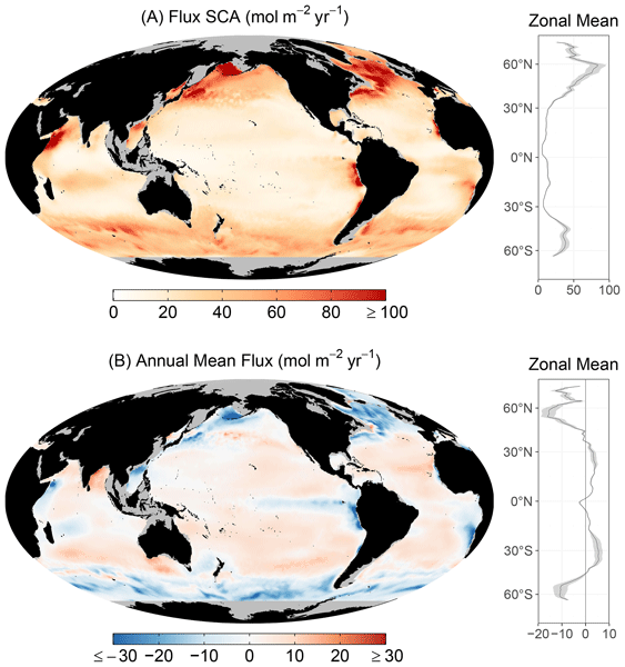
We present gridded seasonal flux climatology maps in Fig. 1, as well as uncertainties in Fig. S2 and monthly zonal-average fluxes (2004–2024 average) in Fig. S3. Our analysis focuses on examining seasonal flux patterns (Sect. 3.1.1) and annual means (Sect. 3.1.2). Figure 2 presents monthly flux climatologies for 18 RECCAP2 regions plus Northern and Southern Hemisphere averages. Figure 3 shows flux seasonal cycle amplitude (SCA), defined as the difference between the maximum and minimum of the fitted seasonal cycle, and annual mean values, presented as both gridded fields and zonal averages with associated uncertainties. Figure 4 compares annual mean fluxes between regions, showing results both with and without annual adjustments. Figure 5 analyzes fractional contributions of each uncertainty source to total flux uncertainty for climatological seasonal cycles and annual means across all 20 regions.
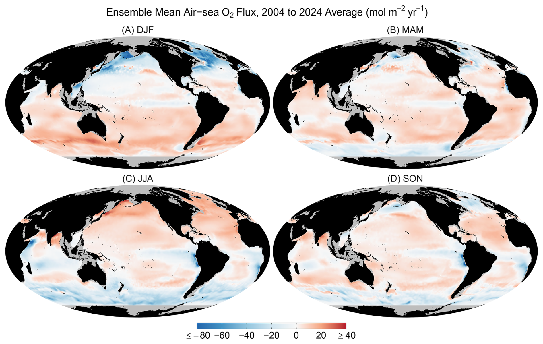
Figure 1Seasonal climatology of ensemble mean air-sea O2 flux over 2004–2024. Seasons shown are (A) December-January-February (DJF), (B) March-April-May (MAM), (C) June-July-August (JJA), and (D) September-October-November (SON). Positive values (red) indicate net ocean O2 outgassing. We show the 1σ uncertainty of the seasonal flux climatology among the 9000 ensemble members in Fig. S2. Gray areas indicate regions where data are unavailable in the GOBAI-O2 v2.3 product. Monthly zonal average fluxes are shown in Fig. S3.
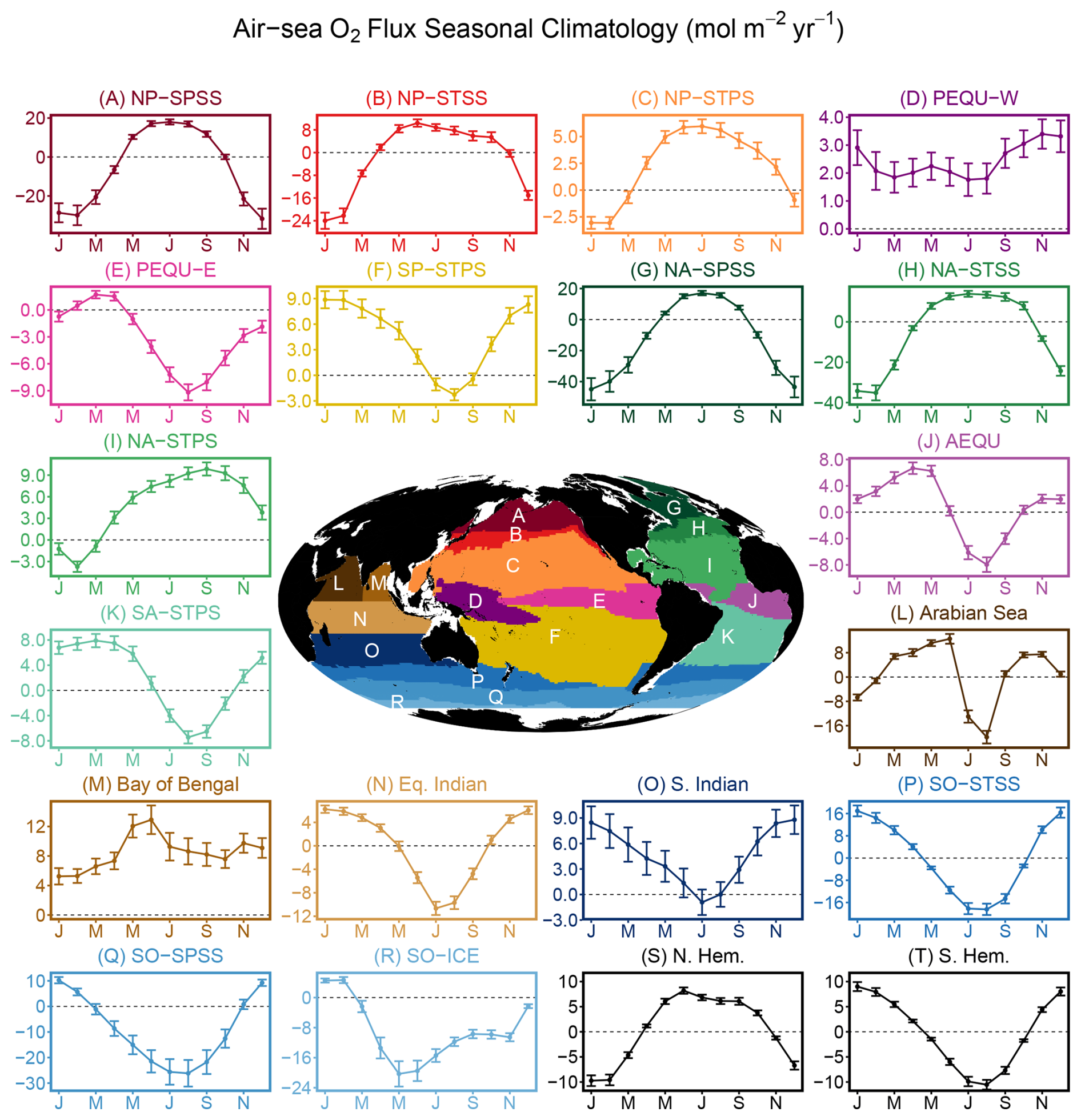
Figure 2Monthly climatology (2004–2024 average) of air-sea O2 flux across 18 RECCAP2 regions and for Northern and Southern Hemisphere averages. The region map is shown in the center, with white areas indicating regions where DO data are unavailable in the GOBAI-O2 v2.3 product. Panels are organized by ocean basins with Pacific regions from (A) to (F), Atlantic regions from (G) to (K), Indian regions from (L) to (O), Southern Ocean regions from (P) to (R), and hemispheric integrals in (S) and (T). Panel titles and colors correspond to the region names and colors shown in the center map. Y axis ranges vary across panels to optimize visualization of seasonal flux amplitude for each region. Error bars represent flux uncertainty estimated from the ensemble standard deviation. Abbreviations include NP (North Pacific), SP (South Pacific), NA (North Atlantic), SA (South Atlantic), SO (Southern Ocean), PEQU (Equatorial Pacific), AEQU (Equatorial Atlantic), SPSS (subpolar seasonally-stratified), STSS (subtropical seasonally-stratified), STPS (subtropical permanently-stratified), and ICE (seasonally ice-covered zone). We show interannual variability of flux SCA in each region in Fig. S5. We compare the flux seasonal cycle with results from two earlier versions of GOBAI-O2 in Fig. S6, which shows generally good agreement but notable differences in the Indian Ocean and subtropical oceans.
3.1.1 Flux seasonal variation
Our air-sea O2 flux exhibits clear seasonal patterns. In each hemisphere (Figs. 1 and 2S–T), there is net outgassing during summer and net uptake during winter, with rapid transitions between seasons. This pattern is consistent with the combined influence of thermal and biological forcing that enhances the seasonal flux cycle. However, the two hemispheres show clear asymmetry in seasonal flux phases (Fig. 2S–T). The Northern Hemisphere exhibits prolonged summer outgassing from mid-April to early November, with a peak in June followed by a broad outgassing plateau through September. In contrast, the Southern Hemisphere shows only a slightly longer outgassing period than its uptake period, without a clear peak and plateau structure. The SCA in the Southern Hemisphere of 19.9 ± 1.86 mol m−2 yr−1 is larger than that in the Northern Hemisphere of 18.1 ± 1.69 mol m−2 yr−1 (Table 1). Our results suggest a similar seasonal flux structure but larger flux SCA in both hemispheres compared to the earlier study of Najjar and Keeling (2000), which reported approximately 15 and 18 mol m−2 yr−1 for the Northern and Southern Hemispheres, respectively. The hemispheric seasonal net outgassing (SNO), defined as the area under the positive portion of the two-harmonic fitted seasonal cycle after removing the annual mean flux, is 363 ± 36 Tmol in the Northern Hemisphere and 584 ± 55 Tmol in the Southern Hemisphere. These values are only slightly larger than the earlier estimates of 322 and 534 Tmol from Najjar and Keeling (2000) and 312 and 549 Tmol from Garcia and Keeling (2001), both of which were based on the hydrographic observations archived by 1994 and 1998, respectively.
Table 1SCA and annual mean values of air-sea O2 flux for 18 RECCAP2 regions and the Northern and Southern Hemispheres. SCA is calculated by first fitting a 2-harmonic function to the climatological monthly data (2004–2024 average), then calculating the difference between the seasonal maximum and minimum. SCA and annual mean fluxes in Tmol yr−1 are the corresponding per-area values in mol m−2 yr−1 multiplied by the area of each region. Region acronyms are defined in Fig. 2.
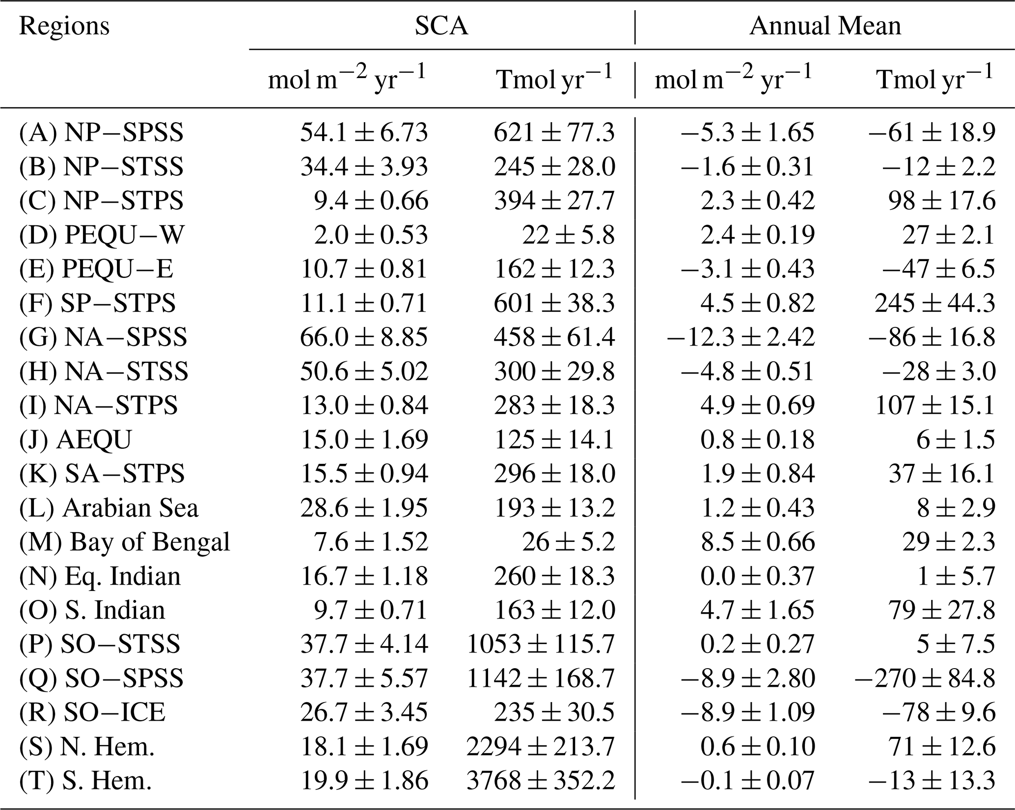
Within each hemisphere, flux SCA is larger at mid-to-high latitudes (Fig. 3A) due to stronger seasonal variations in SST, heat flux, and biological production that drive larger seasonal changes in surface ocean DO. In the Northern Hemisphere, flux SCA peaks at 59.5° N (83.9 ± 11.6 mol m−2 yr−1, Fig. 3A), driven by significant seasonal flux variations over the Western North Pacific and Western North Atlantic (Figs. 2A and G, 3A). SCA is larger over the subpolar North Atlantic (66.0 ± 8.85 mol m−2 yr−1, Fig. 2G) than the subpolar North Pacific (54.1 ± 6.73 mol m−2 yr−1, Fig. 2A) due to stronger wintertime O2 uptake, likely a thermal signal associated with North Atlantic deep-water formation. North of 59.5° N, SCA averages 49.3 mol m−2 yr−1 between 60 and 79.5° N. We note that the O2 flux over the Arctic Ocean and Bering Strait is unavailable in our product due to the lack of GOBAI-O2 data.
Moving southward in the North Pacific and North Atlantic, SCA values decrease from subpolar regions to subtropical regions (Fig. 2B, C, H, I, and Table 1). The onset of net O2 outgassing shifts earlier from high to low latitudes, likely due to earlier bloom onset and thermal changes at lower latitudes. Broad summer outgassing plateaus are evident over both the North Pacific and Atlantic (Fig. 2A, B, H), particularly prominent in Pacific subpolar and subtropical-seasonally-stratified regions (Fig. 2A–B) and the North Atlantic subtropical-seasonally-stratified region (Fig. 2H). These “plateaus” and secondary outgassing peaks result from the formation of a shallow oxygen maximum zone (SOM), which has been observed over the North Pacific (Hayward, 1994; Ishidoya et al., 2016). The SOM forms when strong summer stratification traps photosynthetically produced O2 below the mixed-layer, delaying outgassing until fall when the mixed-layer deepens. At the hemispheric scale, the reduced outgassing after the June peak also partly reflects strong monsoon-driven O2 flux over the Arabian Sea and Bay of Bengal (Fig. 2L and M). Excluding these two from the Northern Hemisphere average removes most of the reduction in summer outgassing.
In the Southern Hemisphere, the zonal mean flux SCA shows two peaks of 38.5 ± 5.7 mol m−2 yr−1 at 54.5° S and 41.0 ± 4.9 mol m−2 yr−1 at 44.5° S (Fig. 3A). Note that flux data south of 64.5° S are unavailable. SCA remains comparably large over the Southern Ocean subpolar region (SO-SPSS, 37.7 ± 5.57 mol m−2 yr−1, Fig. 2Q) and subtropics (37.7 ± 4.14 mol m−2 yr−1, Fig. 2P), although both values are significantly smaller than those in the subpolar North Pacific and North Atlantic. South of this subpolar region, the Southern Ocean seasonally ice-covered zone north of 64.5° S shows reduced SCA (26.7 ± 3.45 mol m−2 yr−1, Fig. 2R) due to winter ice coverage that reduces the net O2 sink. Equatorward, SCA is considerably smaller over permanently-stratified regions, with values of 11.1 ± 0.71 mol m−2 yr−1 in the Pacific (Fig. 2F), 15.5 ± 0.94 mol m−2 yr−1 in the Atlantic (Fig. 2K), and 9.7 ± 0.71 mol m−2 yr−1 in the Southern Indian Ocean (Fig. 2O). As in the Northern Hemisphere, the Southern Hemisphere exhibits earlier phase shifts in outgassing onset and peak timing from high to low latitudes. However, unlike the Northern Hemisphere, the Southern Hemisphere does not exhibit pronounced “summer plateaus”, likely because deeper mixed-layers prevent formation of the SOM (Jin et al., 2023).
Over the equatorial region, the Eastern Equatorial Pacific (Fig. 2E), Equatorial Atlantic (Fig. 2J), and Equatorial Indian Ocean (Fig. 2N) exhibit seasonal flux patterns that generally follow the Southern Hemisphere cycle. However, maximum outgassing occurs approximately three months later in the Equatorial Atlantic (Fig. 2J) and Eastern Equatorial Pacific (Fig. 2E) compared to the Southern Hemisphere pattern. In the Arabian Sea (Fig. 2L), the seasonal flux pattern is dominated by strong O2 uptake associated with monsoon-driven upwelling in summer, while the Bay of Bengal (Fig. 2M) remains a net O2 source throughout the year with reduced outgassing during the monsoon season. The Western Equatorial Pacific (Fig. 2D) shows minimal seasonal flux variation, with persistent O2 outgassing throughout the year. The seasonal cycle over the Eastern Equatorial Pacific is primarily driven by upwelling of cold deep water. A similar upwelling mechanism operates over the Eastern Equatorial Atlantic but with smaller magnitude. In the Arabian Sea and Bay of Bengal, upwelling during the summer monsoon brings cold water to the surface through Ekman-driven vertical transport (Schott and McCreary, 2001).
Our flux estimates show no significant (p< 0.1) SCA trends over most RECCAP2 regions (Fig. S5), except in the North Pacific subpolar seasonally stratified region (Fig. S5A), which exhibits a trend of 3.7 ± 2.2 mol m−2 yr−1 per decade.
Air-sea O2 flux calculations are sensitive to the choice of gas exchange parameterization scheme. Figure A1 shows that flux estimates vary considerably among different schemes, particularly at the high latitudes and during winter when strong winds amplify gas exchange rates. Generally, the L13 scheme produces the smallest SCA due to its calculation of weaker wintertime O2 uptake, while the S09 scheme yields the largest SCA. Over the Southern Ocean subpolar region (Fig. A1Q), the wintertime peak O2 uptake in August varies by approximately 13 mol m−2 yr−1 around an ensemble mean of ∼ 26 mol m−2 yr−1. The impact of parameterization choice is much smaller over low-latitude regions where wind speeds are generally lower.
Flux calculations are less sensitive to the choice of wind product. Figure A2 shows that the hemispheric-scale O2 monthly flux climatologies are highly consistent across the three wind products used. However, larger deviations occur for individual regions. Over the Southern Ocean ice-covered zone (Fig. A2R), JRA-3Q produces the largest wintertime O2 uptake. In other high-latitude regions of both hemispheres, wintertime uptake is larger when using the CCMP wind product, but remains close to the JRA-3Q-based estimate. Over the Bay of Bengal (Fig. A2M), JRA-3Q produces much smaller JJA outgassing compared to the other wind products. These wind products show considerable variation in this region, likely reflecting large uncertainty in surface winds during the monsoon season. Gas exchange uncertainty and wind uncertainty interact nonlinearly, amplifying the total uncertainty. This interaction is particularly pronounced when testing gas exchange schemes with wind products that have faster wind speeds, as gas transfer velocity scales nonlinearly with wind speed.
The annual mean DO adjustment alters the seasonal flux cycle through the interaction between the temporally constant DO adjustments and seasonally varying wind speeds in the gas exchange parameterization (Fig. B3). In the northern high-latitude oceans, where the DO reductions from the adjustment are large and winter wind speeds are much stronger than in summer, the adjustment increases the seasonal cycle amplitude (SCA) by 2 %–5 %. This increase results from enhanced wintertime O2 uptake that exceeds the reduction in summertime outgassing following the adjustment. The largest relative changes occur in the northern Indian Ocean, where the adjustment interacts with the strong summer monsoon winds. The Arabian Sea shows the largest absolute SCA change, an increase of 2.7 mol m−2 yr−1 (10.2 %). In contrast, SCA remains largely unchanged in the southern high latitudes due to the smaller DO adjustments in these regions. Across most regions, the annual mean DO adjustment also reduces the ensemble standard deviation (1σ) of SCA.
We show that the total uncertainty in climatological monthly flux is dominated by either DO uncertainty or gas exchange uncertainty in most regions and months (Fig. 5). In the high-latitude regions of both hemispheres (Fig. 5A, B, G, H, P, Q, R), total uncertainty is dominated by gas exchange uncertainty throughout most of the year, except when net fluxes approach zero, during which DO uncertainty dominates. In mid-latitude subtropical regions of both hemispheres (Fig. 5C, F, I, K, O), gas exchange uncertainty contributes more to total flux uncertainty than DO uncertainty during summer months. In the low-latitude regions (Fig. 5D, E, J, M, N), DO uncertainty generally dominates, especially where lower wind speeds yield consistent flux magnitudes across different gas exchange schemes. Over the ice-covered regions, wind product uncertainty also contributes substantially to total variance. At the hemispheric scale (Fig. 5S, T), fractional variance contributions resemble those at high latitudes, with gas exchange uncertainty dominating because high-latitude seasonal flux cycles drive hemispheric patterns.
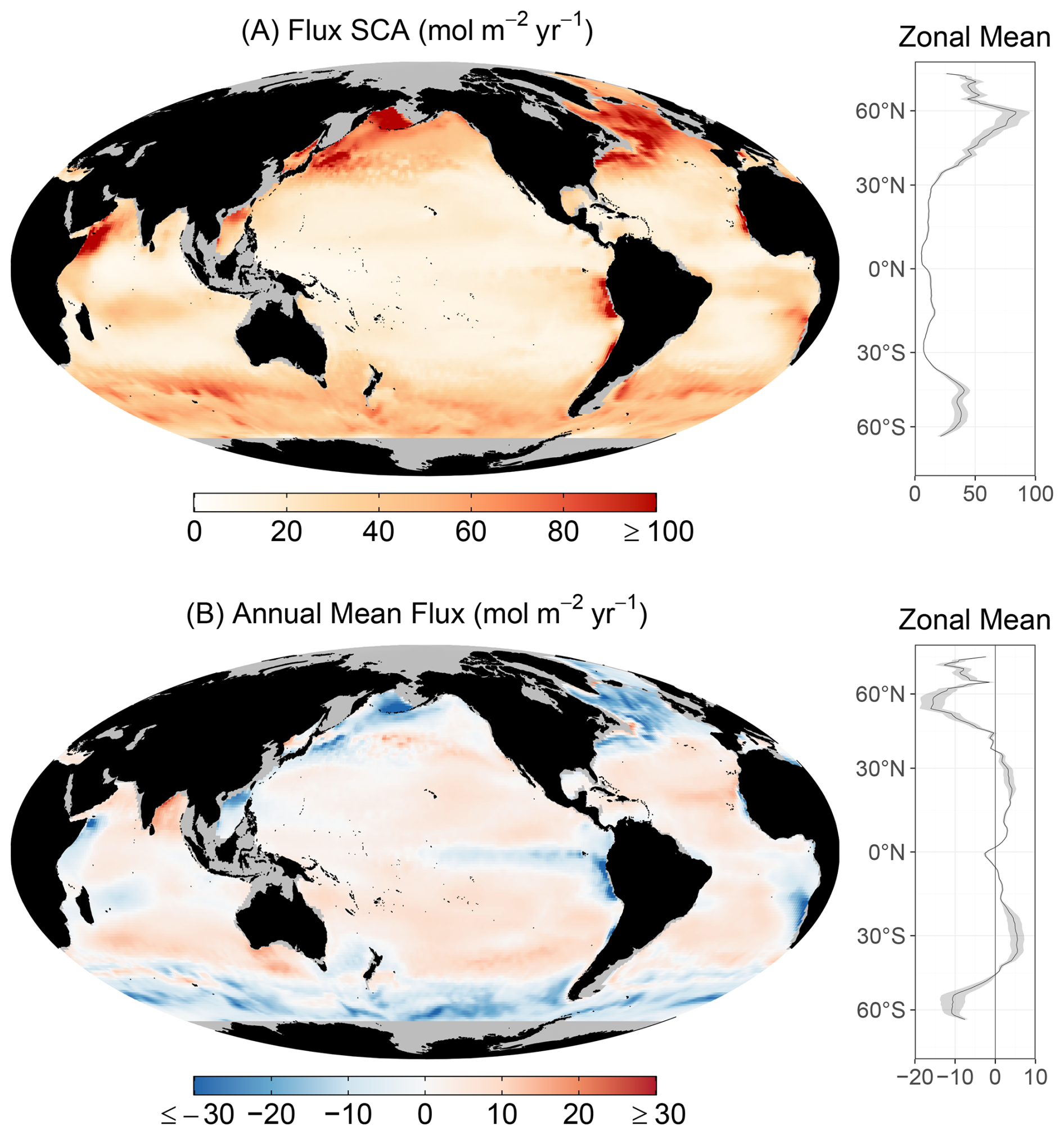
Figure 3Air-sea O2 flux seasonal cycle amplitudes (SCA, A) and annual means (B). Gridded SCA (A) is calculated by first fitting a 2-harmonic function to the climatological monthly data (2004–2024), then calculating the difference between the seasonal maximum and minimum. The corresponding uncertainty is shown in Fig. S4A. Gridded annual mean flux (B) represents the time average of all monthly fluxes, with uncertainty shown in Fig. S4B. Zonal average SCA and annual means are shown on the right, calculated by first computing zonal and annual averages of monthly fluxes for each ensemble member, then fitting the 2-harmonic function (for SCA) or time-averaging (for annual mean). Gray shading represents uncertainty in the zonal mean as the ensemble standard deviation across members.
3.1.2 Flux annual mean
The zonal mean annual flux pattern suggests that the ocean is a strong annual O2 sink at high latitudes, a weak sink at the equator, and a weak source in the subtropics (Fig. 3B). At the hemispheric scale, the Northern Hemisphere acts as a net annual O2 source to the atmosphere (0.6 ± 0.10 mol m−2 yr−1) while the Southern Hemisphere is a net sink (−0.1 ± 0.07 mol m−2 yr−1), as shown in Fig. 4S and T, and Table 1. Over high-latitude regions, the North Atlantic subpolar seasonally stratified region is the strongest regional O2 sink per area (−12.3 ± 2.42 mol m−2 yr−1, Fig. 4G), followed by the subpolar Southern Ocean (−8.9 ± 2.80 mol m−2 yr−1, Fig. 4Q) and the Southern Ocean ice-covered zone (−8.9 ± 1.09 mol m−2 yr−1, Fig. 4R). These regions experience vigorous deep-water formation driven by winter cooling, which increases O2 solubility in cold surface waters and drives convective mixing that efficiently transfers O2 to depth (Koelling et al., 2022). In addition, the upwelling of biologically O2-depleted deep waters in these regions creates surface DO undersaturation that enhances atmospheric O2 uptake (Boyer et al., 1999). The subpolar North Pacific exhibits a weaker sink (−5.3 ± 1.65 mol m−2 yr−1, Fig. 4A) than the North Atlantic, likely due to less vigorous deep convection and different circulation patterns.
Across equatorial regions, the Eastern Equatorial Pacific (−3.1 ± 0.43 mol m−2 yr−1, Fig. 4E) is a weak O2 sink, while the other equatorial regions are O2 sources, including the Western Equatorial Pacific (2.4 ± 0.19 mol m−2 yr−1, Fig. 4D), the Equatorial Atlantic (0.8 ± 0.18 mol m−2 yr−1, Fig. 4J), and the Bay of Bengal (8.5 ± 0.66 mol m−2 yr−1, Fig. 4M). The Eastern Equatorial Pacific experiences strong upwelling of O2-depleted deep water from the oxygen minimum zone below, creating intense surface DO undersaturation that drives atmospheric O2 uptake. The Equatorial Atlantic also experiences upwelling of O2-depleted water, but this uptake is offset by stronger biological productivity that produces O2, resulting in weak outgassing (Brandt et al., 2023). In contrast, the Western Equatorial Pacific is characterized by strong stratification that limits upwelling and receives O2-rich water from the subtropical gyre, leading to surface DO supersaturation and net O2 outgassing (Busecke et al., 2022; Fine et al., 1994).
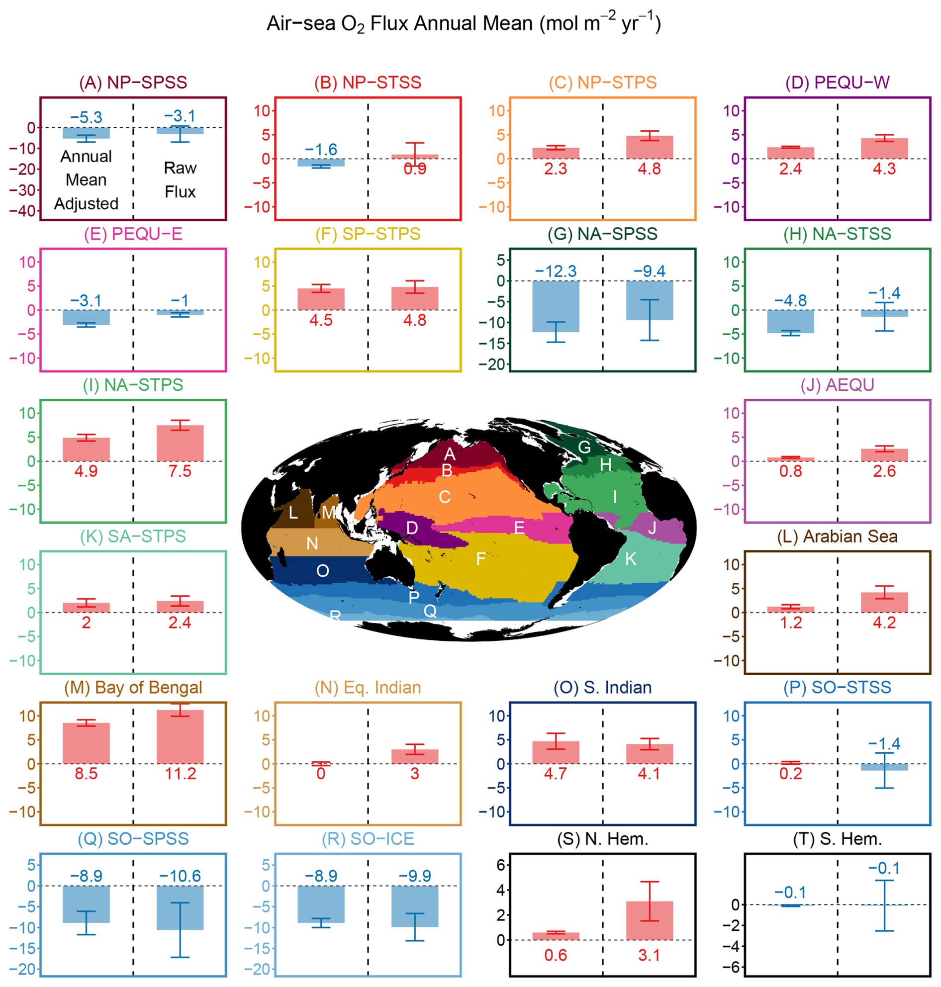
Figure 4Air-sea O2 flux annual mean values for 18 RECCAP2 regions and Northern and Southern Hemisphere averages. For each region, adjusted annual means (left in each panel) are compared with raw flux estimates (right in each panel). Red bars have positive values that indicate net O2 outgassing from the ocean, while blue bars have negative values that indicate net O2 uptake. Error bars represent the standard deviation across the flux ensemble. Ensemble average annual mean flux values are labeled for each estimate and are also reported in Table 1 with 1σ uncertainties. Y axis ranges for the four high-latitude regions (A, G, Q, R) and hemispheric averages (S, T) differ from those in other panels to optimize visualization of their distinct flux magnitudes. We compare the annual mean flux resolved using two earlier versions of GOBAI-O2 in Fig. S7.
The annual mean flux correction through DO adjustment (Appendix B) reduces O2 outgassing in the Northern Hemisphere. Without adjustment, the raw flux calculation yields a global net O2 outgassing of 368 Tmol yr−1, significantly larger than our observational constraint of an average of 61 Tmol yr−1. This correction also reduces hemispheric flux asymmetry from 3.2 to 0.7 mol m−2 yr−1 by scaling down Northern Hemisphere annual flux from 3.1 to 0.6 mol m−2 yr−1, with the Southern Hemisphere annual flux unchanged (Fig. 4S and T, and Table 1). At the regional scale (Fig. 4), the correction reduces O2 outgassing or increases O2 uptake in most RECCAP2 regions except the three Southern Ocean regions (Fig. 4P, Q, and R) and the Southern Indian Ocean (Fig. 4O).
Analysis of fractional variance contributions reveals distinct patterns in annual mean flux uncertainty across spatial scales (Fig. 5). At the hemispheric scale, uncertainty in annual mean flux for both the Northern and Southern Hemispheres is dominated by interactions among DO uncertainty, gas exchange parameterization, and wind products (Fig. 5S and T). At the regional scale, gas exchange parameterization dominates uncertainty in the subpolar regions, the subtropical regions, and the Eastern Equatorial Pacific. In contrast, DO uncertainty dominates flux uncertainty in the Equatorial Atlantic and the Western Equatorial Pacific. The Equatorial Indian Ocean exhibits a unique pattern where wind uncertainty dominates, likely reflecting the strong influence of monsoon-driven wind variability during the northern summer. In the Bay of Bengal and the Arabian Sea, the uncertainty is more evenly partitioned among three sources.
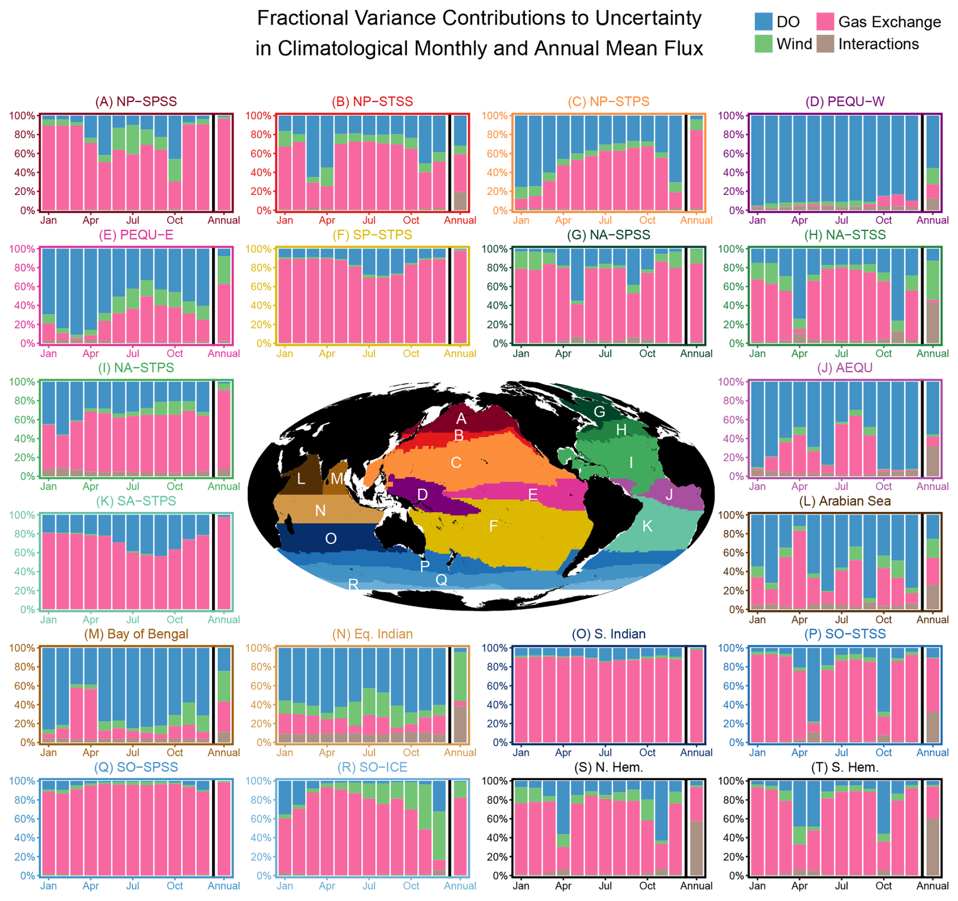
Figure 5Fractional variance contributions to uncertainty in climatological monthly and annual mean O2 flux across global ocean regions. Stacked bar charts show the relative contributions of different uncertainty sources for each month (2004–2024 climatology) and for the annual mean (rightmost bar, 2004–2024 average). Uncertainty sources include variability in DO fields from 1000 ensemble members with annual mean adjustment (blue), three wind products (green), three gas exchange parameterization schemes (pink), and the combined interactions between these three factors (brown). Variance fractional contributions are estimated using a three-way factorial mixed-effects analysis of variance (ANOVA) with the lme4 package in R (Bates et al., 2015).
3.2 Flux evaluation
3.2.1 Flux seasonal cycle
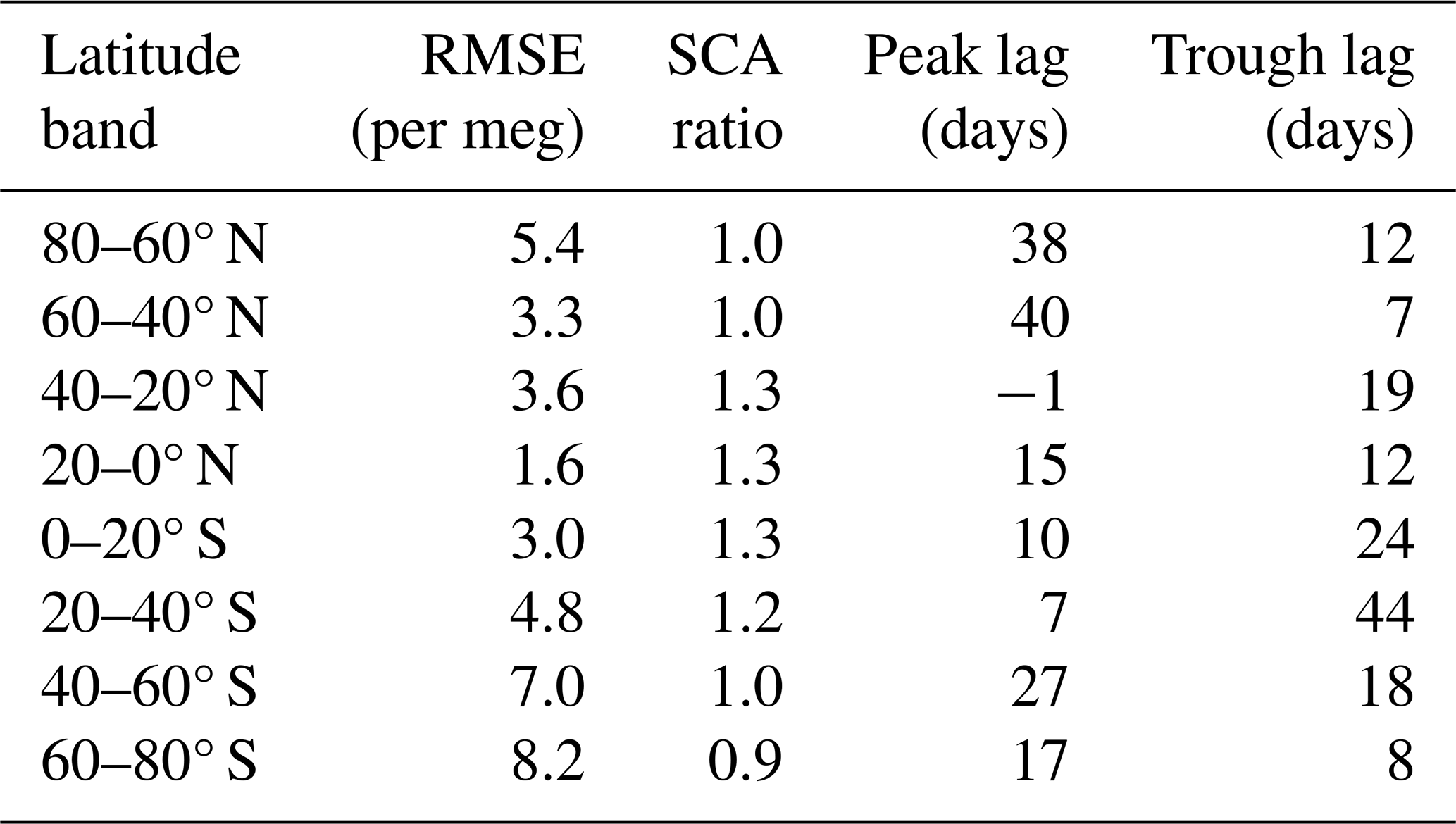
We compare 2-harmonic fits of latitudinally-binned airborne tropospheric-average from TM3 forward transport simulation of ensemble mean fluxes with airborne observations fitted in the same way (Fig. 6). The simulations and observations show good overall agreement. In the northern mid-to-high latitudes (60–80° N), our simulations successfully capture the prolonged outgassing period and the broad, plateau-like summer maximum observed in atmospheric data (Fig. 6), and agree with the observed SCA (Table 2). In the southern mid-to-high latitudes (60–80° S), our simulations underestimate the SCA by 9 %, primarily due to a weak summertime peak. In the low latitudes (20° S–40° N), our simulations generally overestimate SCA by up to 30 %, though this represents a small absolute bias given the weak seasonal cycles in these regions. In the high latitudes of both hemispheres, our simulations lag the observed seasonal peaks by up to 6 weeks, suggesting that peak outgassing occurs too late in the flux product. Simulated seasonal trough timing generally lags observations by one to three weeks, except in the mid-latitude Southern Hemisphere (40–20° S), where the phase lag is much larger, reaching six weeks. The mechanisms driving these phase lags remain unclear and require further investigation, and we cannot rule out a contribution from transport model error given that our simulations use a single transport model (Jin et al., 2025). RMSE (Table 2) is higher in the Southern Hemisphere than in the Northern Hemisphere. The largest RMSE occurs at high southern latitudes (8.2 per meg), which remains much smaller than the seasonal amplitude (73 per meg).
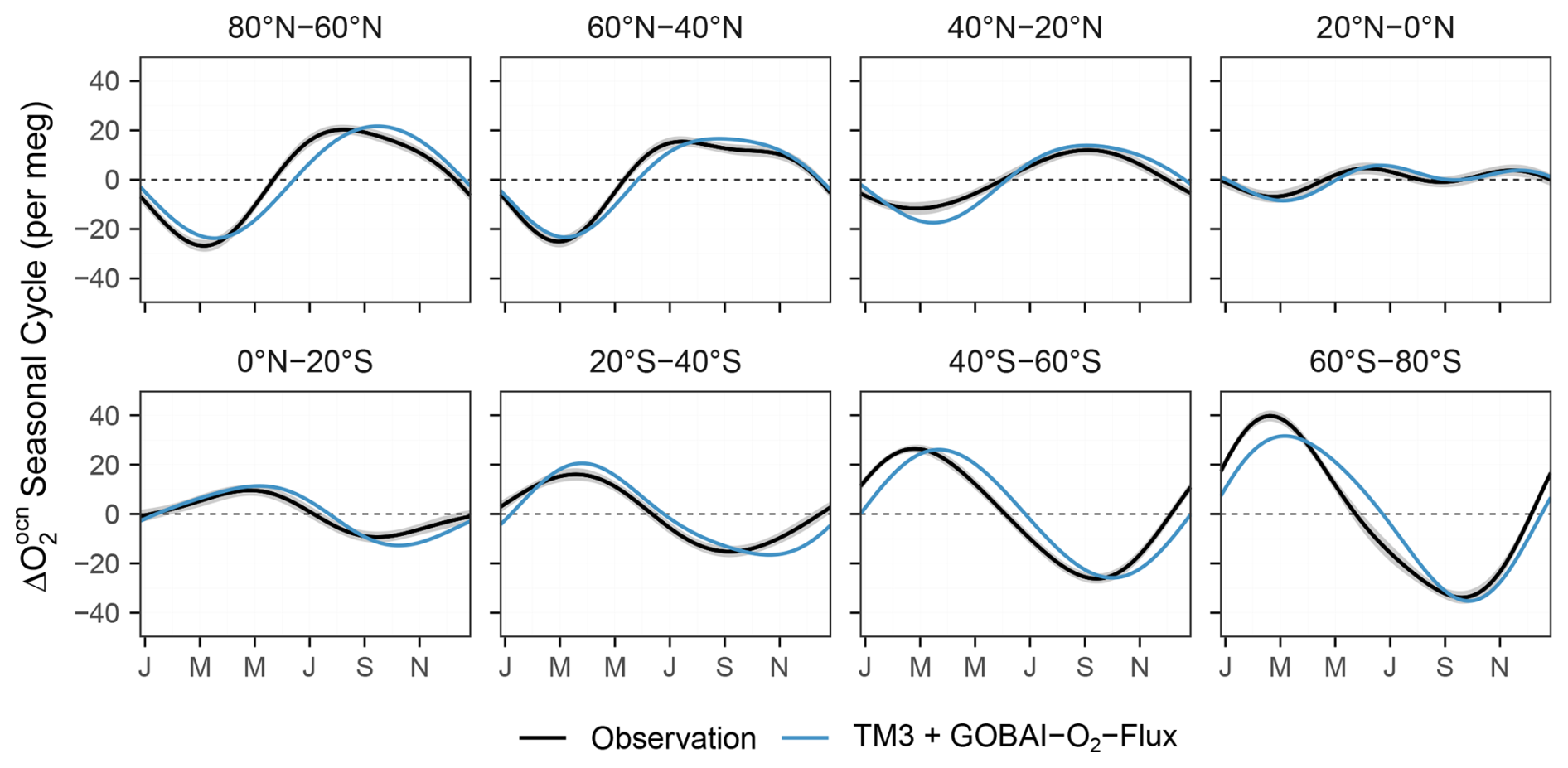
Figure 6Comparison of tropospheric-average (1000 to 400 hPa) seasonal atmospheric between observations and simulations for eight latitude bands from 80° N to 80° S. Observations (black) are derived from airborne APO data corrected for non-oceanic O2 flux components (Appendix C). Model simulations are based on TM3 forward transport of our ensemble mean flux estimates (GOBAI-O2-Flux). The transport model simulations provide co-samplings at each observation time and location, ensuring direct comparison without spatial and temporal sampling bias. Airborne observations and model simulations are first detrended using observed or simulated surface station trends. These surface station trends are determined by linear fits to multiple-station weighted averages following Hamme and Keeling (2008). The detrended airborne observations and model simulations between 1000–400 hPa are then binned by latitude band. Stratospheric data are filtered out based on airborne measurements of water vapor, O3, and N2O (Sect. 2.7). For each latitude band, the seasonal cycle is calculated by applying a 2-harmonic fit to the detrended data after removing the annual mean. Gray shading represents uncertainty in the observed seasonal cycle, combining measurement uncertainty and uncertainty in atmospheric non-oceanic O2 component corrections estimated from an ensemble of flux products and transport models (Appendix C). For each latitude band, Table 2 reports the root mean square error (RMSE), phase lag based on the seasonal peak and trough, and SCA ratio (). A comparison with TM3 forward transport of the GK01 (Garcia and Keeling, 2001) air-sea O2 flux product is shown in Fig. S8. Comparisons of observations with TM3 simulations driven by our fluxes computed using different gas exchange schemes and wind products are shown in Figs. S9 and S10.
Table 2Performance metrics comparing simulated and observed seasonal cycles across eight latitude bands. RMSE (per meg), phase lag (days), and SCA ratios are shown. Positive phase lags indicate that the simulated seasonal cycle lags behind observations. SCA ratio is calculated as simulated SCA divided by observed SCA.
Our hemispheric-scale seasonal flux cycles improve on the widely used GK01 flux product (Garcia and Keeling, 2001), as shown in Fig. S8. GK01 significantly underestimates the flux seasonal cycle at high latitudes in both hemispheres and fails to resolve the prolonged summer outgassing in the northern mid to high latitudes with distinct double-peak structure from 40–60° N. These complex seasonal characteristics in the Northern Hemisphere have been independently confirmed by hemispheric flux estimates derived from atmospheric measurements at both surface stations and from airborne surveys (Jin et al., 2023; Rödenbeck et al., 2008). These patterns are also seen in one configuration of the Community Earth System Model (Yeager et al., 2022). While the simulated seasonal cycle in our flux product generally lags in phase relative to the airborne observations, the simulated seasonal cycle in GK01 leads the observations by 1–2 weeks at mid to high latitudes in the Southern Hemisphere. This phase difference likely reflects the methodological assumption in GK01 that ocean heat flux and O2 flux are in phase.
Forward transport of the ensemble mean flux resolved using each gas exchange parameterization and CCMP winds shows that the L13 scheme produces the smallest simulated SCA, while the S09 scheme produces the largest SCA (Fig. S9), consistent with the order of flux SCA resolved using these three schemes (Fig. A1). A similar test using each of the three wind products with the L13 scheme yields consistent SCA (Fig. S10). Using these airborne data to evaluate the three gas exchange parameterizations and three wind products is complicated by potential biases in DO fields.
It is important to note that, while we use only one transport model, our results are not biased by potential uncertainties in forward transport simulations. Using tropospheric-average atmospheric concentrations as the evaluation metric effectively eliminates potential biases from transport model representations of vertical mixing. The study of Jin et al. (2025) demonstrated that different transport models are highly consistent in simulating tropospheric-average airborne APO but show significant spread at surface stations. Nevertheless, we show that at most surface stations (Fig. S11), model simulations still agree with observations in seasonal amplitude and phase, though consistent phase lags are evident, similar to those observed in the airborne data comparison (Fig. 6). The largest biases occur at LJO and CBA (Fig. S11), both Eastern Pacific coastal sites, likely due to vertical mixing and coastal wind biases in the TM3 model, as reported by Jin et al. (2025).
3.2.2 Annual mean flux
We use long-term trends in at surface stations, isolated from APO measurements by correcting other components (Eq. C1), to evaluate global annual mean air-sea O2 fluxes. As shown in Fig. 7, the observed APO is decreasing at a rate of −11.6 ± 0.4 per meg yr−1. This decline is driven by multiple components, including air-sea CO2 flux, air-sea N2 flux, and fossil fuel burning, all of which contribute negatively to the APO trend. The residual shows a small but highly uncertain increase of 1.3 ± 1.12 per meg yr−1, suggesting a net global ocean O2 outgassing. The trend in annual mean (reported in Fig. 7) thus serves as a metric for evaluating global annual mean O2 flux estimates. Our forward transport simulation, with annual mean flux adjustments derived from ocean heat fluxes, produces a trend of 1.5 ± 0.80 per meg yr−1, in agreement with the observation-based estimate. In contrast, the forward transport simulation using raw fluxes yields a substantially larger trend of 9.7 ± 1.65 per meg yr−1, significantly overestimating the observed trend and highlighting the importance of the annual mean flux adjustment.
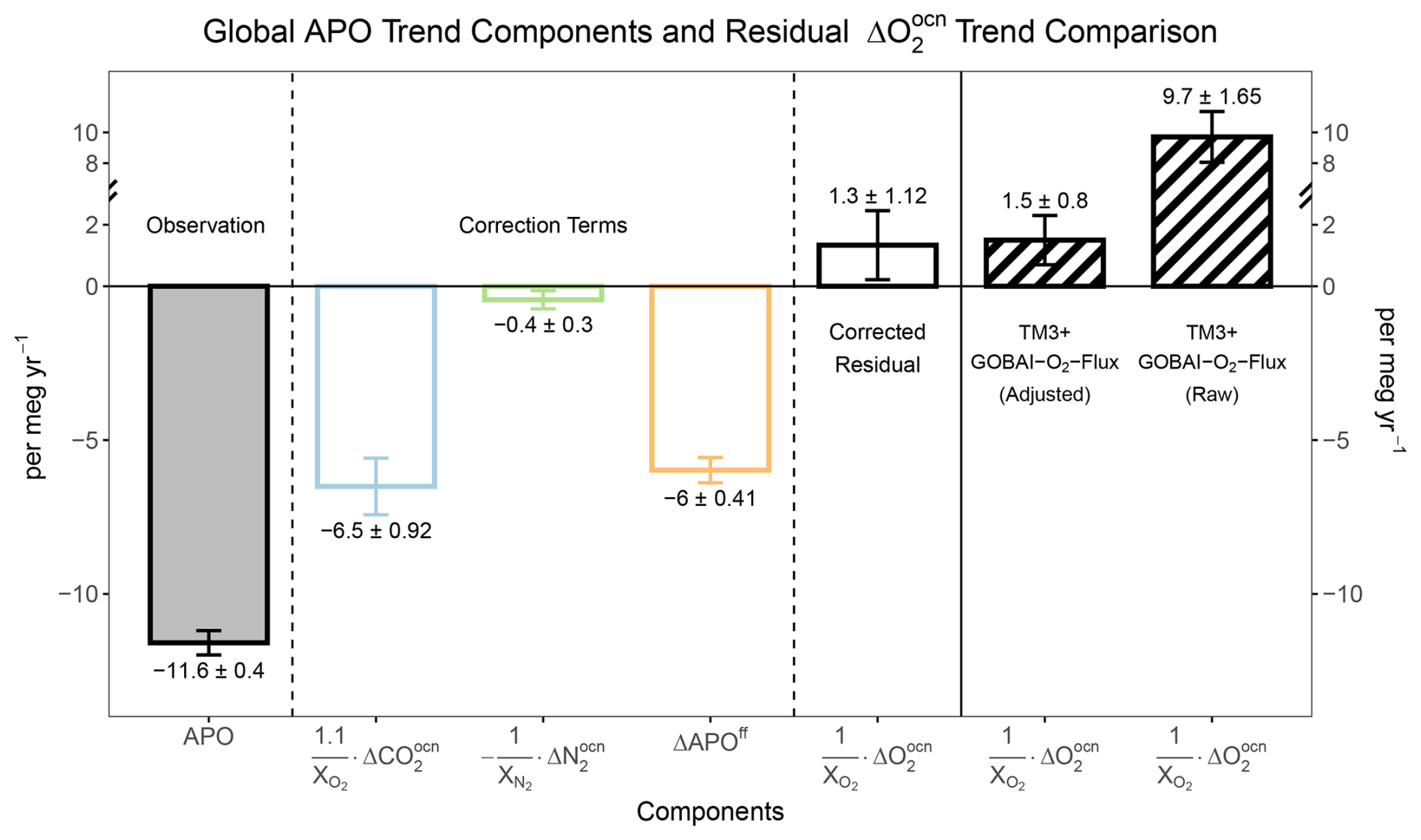
Figure 7Global station-average annual mean APO trend, components that contribute to APO trend, the residual , and comparison to TM3 + GOBAI-O2-Flux model simulations of . Annual mean values of APO and components are calculated as a weighted average of data from seven surface sampling sites across the Pacific basin within the Scripps O2 program (Keeling and Morgan, 2019), with weights following Hamme and Keeling (2008). Correction terms are each flux component forward transported by four atmospheric transport models and sampled at station locations and flask collection times, available from Jin et al. (2025), and further scaled to represent its contributions to the APO trend, following Eq. (C1). Trend is calculated as a linear fit to data from 2005 to 2020. Uncertainty in APO trend is calculated from the station δ(O) error model (Appendix C). Uncertainty in three correction terms is based on the simulated trend calculated using two different flux components and four transport models (8 combinations). Uncertainty in TM3 + GOBAI-O2-Flux simulations is scaled by the uncertainty in annual mean fluxes averaged over 2005 to 2020 divided by the ensemble mean annual flux.
We use airborne observations of tropospheric-mean annual-mean for eight latitude bands spanning 80° S to 80° N to evaluate the meridional gradient of annual mean O2 fluxes (Fig. 8). In the Northern Hemisphere, the meridional gradient is larger in simulations (∼ −0.14 per meg per degree latitude, positive northward) than in observations (−0.07 ± 0.01 per meg per degree latitude). This overestimation is largely due to the absence of an observed rebound at 60–80° N in the simulations. In the Southern Hemisphere, the simulated meridional gradient (0.13 per meg per degree latitude) is much larger than the observed gradient (0.04 ± 0.02 per meg per degree latitude). These biases in both hemispheres produce an overly strong simulated “equatorial bulge” and annual mean values that are too low, relative to the global mean, at high southern latitudes.
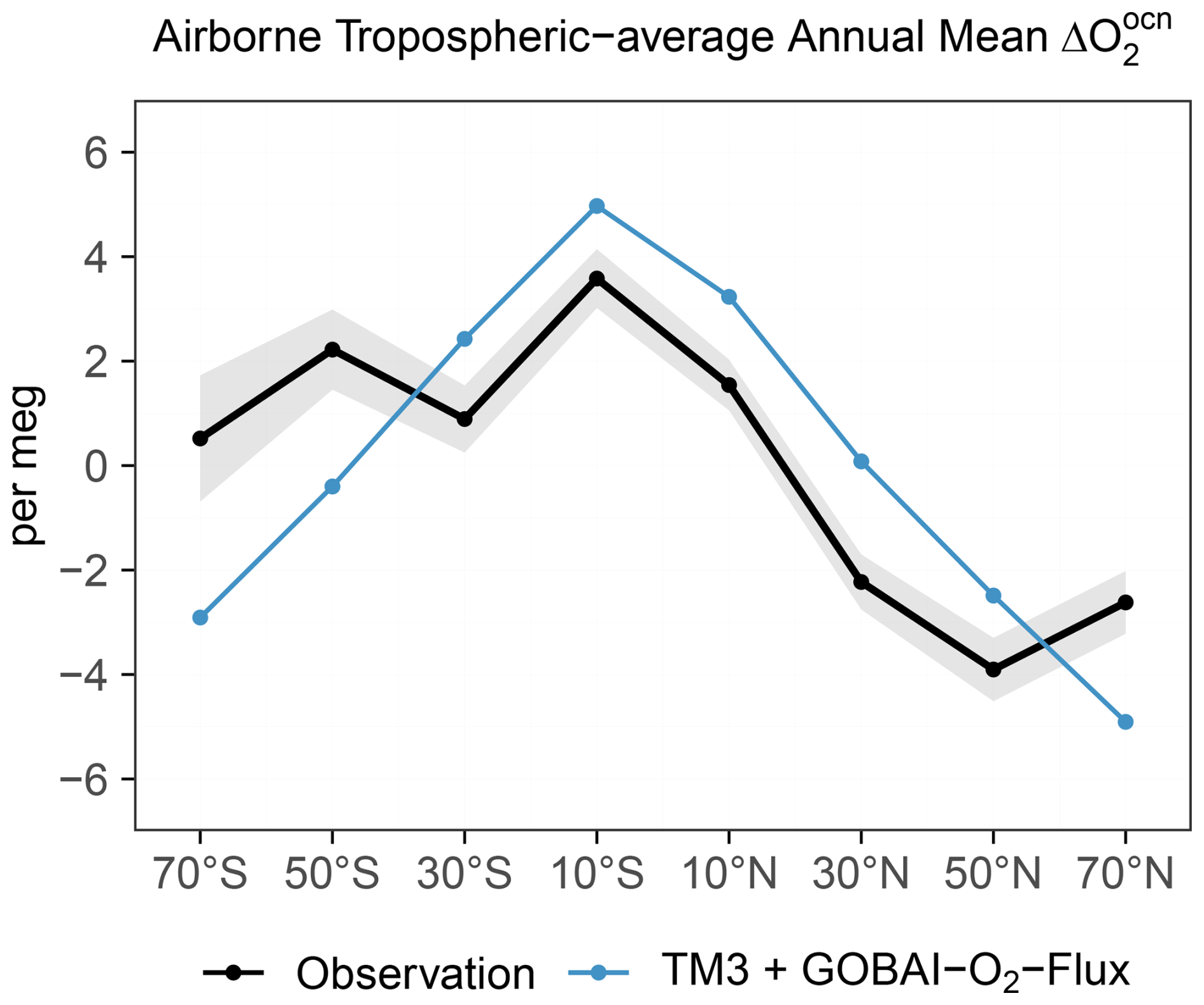
Figure 8Comparison of the meridional gradient in airborne tropospheric-average annual mean between observations (black) and TM3 + GOBAI-O2-Flux simulations (blue) for eight latitude bands spanning 80° N to 80° S at 20° intervals. Data processing, including detrending, binning, and filtering, follows the same procedure described in the Fig. 6 caption. For each latitude band, the annual mean value is calculated by applying a two-harmonic fit with constant offset to the detrended data, and using the offset to represent the annual mean value. The global mean, averaged across all eight latitude bands, is subtracted to center the global annual mean in both lines at 0. Because model simulations have arbitrary global mean values before this subtraction, only the meridional gradient of the annual mean values should be interpreted, rather than the absolute values. Gray shading represents uncertainty in the observed annual mean values, combining measurement uncertainty and uncertainty in the atmospheric non-oceanic O2 component corrections estimated from an ensemble of flux products and transport models (Appendix C).
Biases in the annual mean meridional gradients indicate that regional annual mean flux constraints from the ocean inversions (Resplandy et al., 2016) overestimate either or both O2 outgassing in the equatorial region and O2 uptake at high southern latitudes. Nevertheless, applying these constraints improves flux estimates by reducing the meridional flux gradient, particularly in the Southern Hemisphere, from 0.36 to 0.13 per meg per degree latitude (not shown). Specifically, the adjustment reduces equatorial outgassing by lowering the annual mean DO (Fig. B2). Earlier studies highlighted similar strong flux “tropical bulges” evident in other ocean inversion products (Battle et al., 2006; Gruber et al., 2001), and in prognostic ocean biogeochemistry models (Stephens et al., 1998). However, previous observational studies do not support this bulge, or only show a small bulge (Pickers et al., 2017; Stephens et al., 1998; Tohjima et al., 2012). The airborne observations shown in Fig. 8 similarly preclude a large equatorial bulge, showing only a small (∼ 3 per meg) enhancement from 0–20° S relative to 60–80° S.
4.1 Data gaps
Our flux calculations are limited by spatial data gaps in GOBAI-O2 DO fields. We could not resolve flux estimates over the Arctic (north of 79.5° N), parts of the Southern Ocean seasonally ice-covered zone (south of 64.5° S), and most coastal regions due to these regions not being included in the GOBAI-O2 products. These regions account for approximately 18 % of Northern Hemisphere oceans and 8 % of Southern Hemisphere oceans, collectively representing 14 % of the global ocean area. Simple area scaling has been used to correct pCO2 products for similar issues (Friedlingstein et al., 2025), but this approach is limited by these regions likely having unique fluxes.
High-latitude polar regions exhibit distinct seasonal variations in physical and biogeochemical processes due to extreme light and temperature cycles, suggesting large seasonal cycles in air-sea O2 flux. Atmospheric O2 observations collected at surface stations and along ship transects confirm significant seasonal variation in these regions (Ishidoya et al., 2016; Jin et al., 2025; Stephens, 2025). The absence of flux estimates from these polar regions likely leads to underestimation of the true seasonal amplitude in regional to hemispheric seasonal flux cycles. TM3 forward transport simulations indicate that flux SCA in the high southern latitudes is underestimated (Fig. 6), likely influenced by the lack of GOBAI-O2 data south of 64.5° S, where summertime blooms could be underrepresented.
Similarly, the absence of coastal data limits our representation of nearshore processes that exhibit intense seasonal biogeochemical activity due to coastal upwelling and riverine nutrient inputs. Satellite-based chlorophyll a data reveal significant blooms in coastal regions, for example, east of the South American coast (Behrenfeld et al., 2005). In contrast, most estuaries are net heterotrophic, oxidizing organic matter delivered from land in excess of their local production, and are therefore more likely to act as O2 sinks (Herrmann et al., 2015). Without O2 flux estimates over these regions, we potentially miss summer-time O2 outgassing events associated with high biological productivity and net O2 uptake by heterotrophic estuarine and other coastal systems.
Here we explore the contribution of these data gaps to area-integrated flux seasonal cycles in the Northern Hemisphere and Southern Hemisphere using a Community Earth System Model version 2 (CESM2) Forced Ocean-Sea-Ice (FOSI) simulation (Yeager et al., 2022), which uses the POP2 ocean model at nominal 1 degree horizontal resolution with 60 vertical levels and includes riverine inputs of nutrients, dissolved inorganic carbon, alkalinity, and dissolved organic matter (Danabasoglu et al., 2020), although nearshore processes remain coarsely resolved at this resolution. This model was evaluated as providing a reasonably good global air-sea O2 flux (Jin et al., 2023, 2025). By excluding GOBAI-O2 data-gap grid cells from the CESM2 output, the 2011–2020 average seasonal flux amplitude is reduced from 14.9 to 14.2 mol m−2 yr−1, and from 16.1 to 15.1 mol m−2 yr−1 in the Northern and Southern Hemispheres, respectively.
Spatial data gaps also introduce uncertainties in annual mean flux estimates. We assume zero flux and zero annual DO adjustment over these gaps. This ensures that extratropical annual mean fluxes match the ocean-inversion constraints. However, this assumption may spatially bias regional estimates by assigning compensatory fluxes to resolved areas. We also explore the contribution of these data gaps to area-integrated annual mean fluxes in the equatorial region (20° S–20° N), northern extratropics (> 20° N), and southern extratropics (< 20° S) using CESM2. The 2011–2020 average equatorial outgassing decreases from 214 to 191 Tmol, northern extratropical ingassing increases from 55 to 56 Tmol yr−1, and southern extratropical ingassing decreases from 45 to 37 Tmol yr−1. This calculation indicates that our zero-flux assumption overestimates tropical outgassing and southern ingassing in resolved regions to compensate for missing fluxes.
The same simulation allows us to assess the effect of computing fluxes from monthly mean DO fields, which neglects the sub-monthly covariance between the gas transfer velocity and the DO anomaly. We note that the averaging of wind speeds to monthly is treated separately in our flux calculation, which uses the monthly mean of the squared wind speed, computed from high-resolution winds as the squared monthly mean plus the intra-month variance (Sect. 2.3). Here we reconstruct the CESM2 flux from monthly mean transfer velocity, DO anomaly, and ice fraction and compare it to the flux accumulated from daily model output over 2004 to 2020 (Figs. S14–S15). Because gas exchange in CESM2 is quadratic in wind speed, the monthly mean of the daily transfer velocity is identical to one computed from the monthly mean of the squared wind speed, so the reconstruction contains no wind speed averaging bias and its difference from the daily accumulated flux arises only from the covariance term. The monthly reconstruction omits a positive covariance term equivalent to 34 ± 4 Tmol yr−1 of additional global outgassing. It also overestimates the flux SCA by up to 9 % in subpolar regions and 10 % in the Bay of Bengal, and by 6 % (NH) and 4.5 % (SH) at the hemispheric scale, with peak months unchanged (Fig. S14). The monthly flux slightly overestimates the meridional gradient of annual mean flux by deepening the 45° S to 65° S sink and overestimates the equatorial outgassing peak by about 7 % (Fig. S15). In our product, the global annual mean is constrained to observation-based values, so the annual mean covariance effect is effectively absorbed by the annual adjustment, while the seasonal effects implied by CESM2 are smaller than our reported ensemble spread (Table 1). We do not apply model-based correction and instead document this effect as a known limitation of monthly flux products.
4.2 DO machine-learning interpolation methods
Our flux estimates might be limited by potential systematic biases in GOBAI-O2 DO fields arising from the ML methodology. Here we employ the latest GOBAI-O2 version v2.3. Alternatively, we resolve fluxes using two earlier versions v2.1 and v2.2, which use slightly different ML methodologies (Sect. 2.1). While hemispheric-scale O2 flux seasonal climatologies remain consistent across all three versions (Fig. S6), regional discrepancies emerge, especially over the Indian and equatorial regions, where sparse observations make reconstructed DO fields sensitive to methodological differences.
We find large deviations in uncorrected regional to global annual mean fluxes across three versions of GOBAI-O2 (Fig. S7). While v2.3 suggests a 368 Tmol yr−1 annual outgassing, v2.1 (2004–2022 average) indicates a net O2 uptake of 1363 Tmol yr−1 and v2.2 (2004–2023 average) shows a net O2 uptake of 915 Tmol yr−1. These strong O2 uptake estimates in v2.1 and v2.2 result from a combination of stronger O2 sinks in the Southern Hemisphere and weaker O2 sources in the Northern Hemisphere compared to v2.3 (Fig. S7S and T), indicating that the annual flux is particularly sensitive to small perturbations in DO. The global annual flux from these two earlier versions also significantly deviates from our heat flux constraint of an average of 61 Tmol yr−1. Although our heat flux constraint removes spread in global annual mean flux resolved across DO versions, large differences in regional annual mean flux persist even after adjustment (Fig. S7).
We compute fluxes from MLD-averaged DO because the flux integrated over a month exchanges with the entire mixed layer, which overturns many times within a month, whereas monthly mean DO at a fixed shallow surface layer inherits transient near-surface stratification and reconstruction noise that do not represent the reservoir engaged in gas exchange. In a single year test (2015) in which fluxes are instead computed from DO at the shallowest GOBAI-O2 level (2.5 m), the hemispheric flux SCA decreases by roughly 20 % and the strong wintertime O2 uptake at high latitudes weakens substantially, for example, from 63 to 31 mol m−2 yr−1 in the North Atlantic subpolar region in January. These differences lead to a worse agreement with airborne observations shown in Sect. 3.2. The constrained global annual mean flux is insensitive to this choice. We also tested the sensitivity to the MLD criterion by recomputing fluxes with the alternative temperature criterion of De Boyer Montégut et al. (2004), which increases the hemispheric SCA by 4 % (NH) and 7 % (SH) and changes the regional SCA by a median magnitude of 6 %, indicating that our results are robust to the MLD criterion choice.
The DO method uncertainty in GOBAI-O2 depends on the distribution of available training data and the ability of ML algorithms to represent underlying system variability, with larger uncertainties in regions of high natural variability and sparse sampling (Fig. 5). High uncertainties could also occur where water masses with similar physical characteristics but different oxygen signatures mix, highlighting challenges in distinguishing biogeochemical from physical drivers using available training parameters. While ML reconstructions provide spatially and temporally complete datasets, they may exhibit smoothing effects that dampen extreme surface ocean DO values critical for accurate flux estimates on short timescales. The monthly temporal resolution may also fail to resolve episodic events that significantly contribute to regional flux budgets. Examples include ocean heat waves that lead to low oxygen extremes (Li et al., 2024), storm-induced deep mixing events that induce surface cooling and potentially draw-down of surface DO and also phytoplankton blooms afterwards (Walker et al., 2005), and episodic phytoplankton blooms induced by dust deposition over the Indian Ocean (Banerjee and Kumar, 2014). Furthermore, ML models are inherently limited by their training data, meaning poorly-represented processes or conditions may not be accurately captured in reconstructions.
GOBAI-O2 integrates observations from both ship-based measurements and Argo floats, and therefore, offsets between these platforms and between ships could introduce systematic biases in reconstructions, requiring more careful strategies to synthesize these datasets (Bushinsky et al., 2025). The latest v2.3 has applied corrections to Argo measurements to minimize systematic biases.
We note that there are other gridded global ocean DO products available that could be used to calculate air-sea O2 fluxes. Ito et al. (2024) provide monthly mean DO fields from 1965–2020 at 1° × 1° resolution from pole to pole and from surface to 1000 m depth. This product uses neural networks and random forest regression to construct DO fields by relating historical data from ship-based measurements (bottle and CTD-O2) and BGC-Argo profiles (after 2005) to climate, spatial, and temporal variables. Gouretski et al. (2024) provide monthly mean DO fields from 1960 onward at 1° × 1° resolution from pole to pole and from surface to 6000 m depth. This product applies enhanced quality control procedures to data from bottle, CTD, and Argo float measurements, then uses a mapping method (Cheng et al., 2017) to spatially interpolate oxygen data. While these products offer valuable DO fields, we chose GOBAI-O2 because it provides detailed, source-specific uncertainty estimates that facilitate quantifying flux uncertainty through large ensembles. Additionally, our goal is to illustrate the feasibility of calculating air-sea O2 fluxes from ML-based DO products rather than to conduct a full intercomparison of different observational products. Nevertheless, future studies could focus on calculating fluxes using different products and quantifying differences in flux estimates arising from distinct methodologies.
4.3 Gas exchange parameterization
Robust O2 flux calculations through gas exchange parameterization require a better understanding of bubble-mediated flux processes. An earlier study identified that in the Labrador Sea, two-thirds of annual oxygen uptake occurs over only 40 d in winter due to bubble-mediated air-sea gas transfer under high wind and deep convection conditions (Atamanchuk et al., 2020). For individual regions, the ensemble mean flux calculated using each gas exchange scheme shows significant uncertainty, especially over high-latitude regions in winter, leading to large spread in annual mean flux estimates (Fig. A1). These wintertime flux anomalies largely shape the seasonal flux cycle. Our flux seasonal cycle evaluation (Fig. 6) reveals certain errors (i.e., RMSE) at high latitudes.
Recent advances in gas exchange theory offer promising improvements for future studies. The universal wind-wave-bubble formulation developed by Deike et al. (2025) explicitly accounts for asymmetric bubble-mediated fluxes through wave breaking statistics. This approach has demonstrated improved representation of DO concentrations in Pacific Subantarctic Mode Waters during their formation period in winter (August–September), suggesting it could substantially reduce uncertainties in regional O2 flux estimates, particularly in high-latitude winter conditions where bubble processes dominate.
4.4 Annual mean flux
Our study shows the annual mean O2 flux estimates remain the largest uncertainty. Reducing this uncertainty is critical for using atmospheric O2 and CO2 observations to constrain land and ocean carbon partitioning through budget equations (Bender et al., 2005; Friedlingstein et al., 2025; Keeling and Manning, 2014). Future research should focus on resolving annual mean fluxes and their interannual variability by improving ocean interior DO reconstructions and developing independent constraints that capture interannual flux variations.
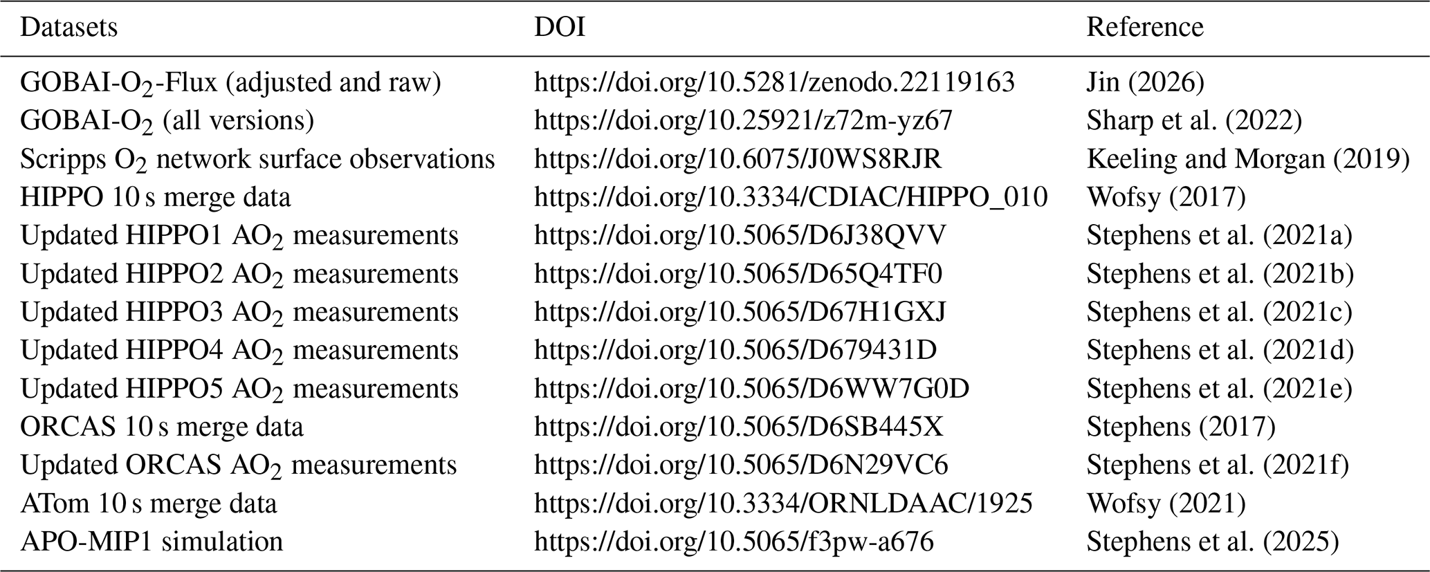
All datasets used in this study are listed in Table 3 with their DOIs.
We develop a gridded product of monthly open ocean air-sea O2 flux from 2004 to 2024 on a 1° × 1° grid, leveraging ML-based DO data products (GOBAI-O2), combined with three gas exchange parameterization schemes and three wind products. By incorporating a large ensemble approach to quantify uncertainties and applying regional adjustments to align annual mean fluxes with those derived from scaling ocean heat flux and from ocean inversions, our product provides a robust representation of air-sea O2 fluxes. This dataset captures pronounced seasonal variability across latitude as well as the global annual mean flux. However, the meridional annual mean flux pattern is biased toward excessive ingassing in the high southern latitudes and too large outgassing in the equatorial region. Our results also reveal distinct basin-scale differences in both flux patterns and seasonal amplitudes.
At the hemispheric scale, our flux estimates reveal the expected seasonal pattern of net oceanic outgassing during summer and net uptake during winter, driven by the combined effects of thermal solubility changes and seasonal biological productivity cycles (Figs. 1–3). Significant asymmetries exist between hemispheres, with the Northern Hemisphere exhibiting prolonged summer outgassing periods lasting seven months and characteristic peak and plateau structures that reflect complex interactions between mixed-layer changes and biological productivity, as well as impact from the northern Indian Ocean monsoon. Regional flux analysis reveals strong flux seasonal variations in subpolar regions, with the North Atlantic subpolar zone and the high-latitude SO showing the most intense flux amplitudes due to deep-water formation (Bushinsky et al., 2017; Koelling et al., 2022; Silva et al., 2024) and extreme thermal cycling. Our global annual mean constraint forces the global ocean to be a weak source of O2 (Figs. 3–4). On the regional scale, strong sinks dominate at high latitudes where cold water formation and upwelling of oxygen-depleted deep waters create persistent undersaturation, while weak sinks characterize equatorial upwelling zones where oxygen-poor waters reach the surface (Eddebbar et al., 2017). In contrast, weak sources occur in subtropical gyres and in the off-equator tropics (e.g., 5 to 20°) where warm, stratified conditions and biological productivity combine to create surface supersaturation and net outgassing to the atmosphere.
Our uncertainty analysis reveals distinct patterns in the dominant sources of flux uncertainty that vary by both geographic region and temporal scale (Fig. 5). For monthly climatological fluxes, gas exchange uncertainty dominates at high latitudes due to the large spread in bubble-mediated flux estimates under high wind conditions, where different parameterization schemes show substantial disagreement in their representation of air injection processes. In contrast, DO uncertainty controls flux uncertainty in low-latitude regions, particularly in areas with sparse observational coverage where ML reconstruction methods struggle to accurately represent the true spatial and temporal variability of ocean biogeochemistry. The annual mean flux uncertainty follows similar geographic patterns for individual regions, but at the hemispheric scale becomes dominated by complex interactions between DO, gas exchange parameterization, and wind uncertainties. We note that, in the adjusted product, part of the variance attributed to DO originates in the annual mean flux adjustment itself. The adjustment is applied as an offset to DO that is drawn independently for each ensemble member, so that member-to-member spread is absorbed into the DO term of the variance decomposition (Fig. 5) rather than appearing as a separate source.
We evaluate our flux estimates by comparing forward transport simulations with global atmospheric O2 observations that have been corrected for non-oceanic O2 flux contributions (Figs. 6–8). For seasonal cycles, our results show good agreement with airborne tropospheric-average observations, though we find systematic overestimation of SCA at low latitudes and underestimation of SCA at high southern latitudes (Fig. 6 and Table 2). We also find that seasonal maximum timing lags observations by about a month in high latitudes of both hemispheres, and the seasonal minimum timing lags observations across all latitudes, with particularly large lags of six weeks in southern mid latitudes (40–20° S). On annual mean timescales, the agreement between simulated and observed long-term atmospheric trend supports the reasonableness of our constrained global annual mean flux of an average of 61 Tmol yr−1 (Fig. 7). However, this observational constraint has large uncertainty due to its sensitivity to the other components used to isolate from APO measurements (Fig. 7). Meridional gradients in annual mean atmospheric concentrations reveal regional biases, with simulations showing excessive in tropical regions relative to high latitudes, suggesting overestimated extratropical ocean uptake and overestimated tropical outgassing in the ocean inversions used to adjust our annual mean flux estimates (Fig. 8).
This dataset represents a significant advance over existing air-sea O2 flux products by resolving interannual variability in the seasonal cycle of the flux, utilizing sophisticated ML-based DO fields that better capture complex spatial and temporal patterns, and providing comprehensive uncertainty quantification across multiple scales. Despite these advances, several opportunities remain for further improvement, including incorporation of high-latitude Arctic and coastal DO estimates that are currently absent from GOBAI-O2 products, collection of DO data in underrepresented areas (e.g., Indian Ocean and high-latitudes), continued development of ML algorithms to better handle sparse and heterogeneous ocean observations, and refinement of bubble-mediated flux parameterizations. The resulting flux product offers substantial value across multiple research communities and applications. It can be used to improve atmospheric inversions on terrestrial and oceanic carbon cycles. It can serve as critical benchmarks for evaluating ocean biogeochemical models and atmospheric transport models. We provide this product for community use.
The W97 method determines the net air-sea O2 flux (FT, mol m−2 s−1) by combining the surface skin and bubble-mediated fluxes, following
where Δ[O2] and [O] (µmol kgsw−1) are defined in Eqs. (5)–(6). ks and kb (m s−1) are the gas exchange velocity due to surface skin and bubble processes, respectively. Δe is the bubble-induced supersaturation, according to Woolf and Thorpe (1991). ρw (kg m−3) is the seawater density as a function of temperature and salinity and is evaluated at the MLD average. The factor of 10−6 is to convert the unit from µmol to mol. Here, we calculate
where (m s−1) is the friction velocity on the air side of the air-water interface, and is calculated based on the unitless drag coefficient (Cd) and 10 m wind speed (U10) following
and is the unitless Schmidt number for O2, calculated as a function of temperature with skin temperature correction (Sect. 2.3), following the method of Wanninkhof (2014). We note that U10 used here retains the effect of sub-monthly wind variability (Eq. 2).
kb is calculated following
in units of cm h−1 and then converted to m s−1 by dividing by 360 000.
Δe is calculated following
where is the reference 10 m wind speed at which Δe is 1 % for O2, and is assumed to be 9.6 m s−1, according to Woolf and Thorpe (1991).
For the L13 and S09 methods, the net flux calculation follows Eqs. (3)–(4). The surface skin flux (Fs) is calculated following
with
for the L13 method, and
for the S09 method.
In these two methods, Fc is calculated as the product of a mass transfer coefficient (kc, mol m−2 s−1) and O2 atmospheric dry-air mole fraction (), following
while Fp is calculated following
with kp (m s−1) as the gas exchange coefficient across the large bubble interface, and ΔP as the bubble-produced increment of supersaturation.
For the L13 method, we have
In Eqs. (A12)–(A14), (m s−1) represents the water-side friction velocity, and is calculated as
For the S09 method, we have
In Eqs. (A12) and (A16), Pa (Pa) is the atmospheric pressure at the sea surface from the ERA5 monthly mean (Hersbach et al., 2020), P0 is the reference pressure of 101 325 Pa, and (Pa) is the equilibrium water vapor pressure, calculated as a function of temperature (Bolton, 1980), following
where Ts (°C) is the temperature of the shallowest GOBAI-O2 level at 2.5 m. The scaling factor 100 converts the unit from hPa to Pa. (m2 s−1) in Eq. (A17) is the molecular diffusion coefficient for O2, with values of 2 × 10⁻⁹ at 20 °C and 1.25 × 10⁻⁹ at 0 °C, and is assumed to vary linearly with temperature. D0 (m2 s−1) in Eq. (A17) is used to ensure unit balance and is equal to 1. R (m3 Pa mol−1 K−1) is the gas constant, assumed to be 8.314. T (K) is surface ocean temperature. For 10 m wind speeds below 2.27 (m s−1), kc and kp are set to 0. zb (m) is the mean depth of large bubbles, calculated as a function of 10 m wind speed, following
with negative zb set to be 0.
The Bunsen coefficient for O2 (β) is determined from temperature (K) and salinity (PSU) using the empirical relationship of Weiss (1970), following
where A1= −58.3877, A2=85.8079, A3=23.8439, B1= −0.034892, B2=0.015568, and B3= −0.0019387.
To illustrate flux differences from varying gas exchange parameterization schemes and wind products, we show monthly climatologies with different parameterization schemes (Fig. A1, using CCMP wind) and different wind products (Fig. A2, using the L13 scheme).
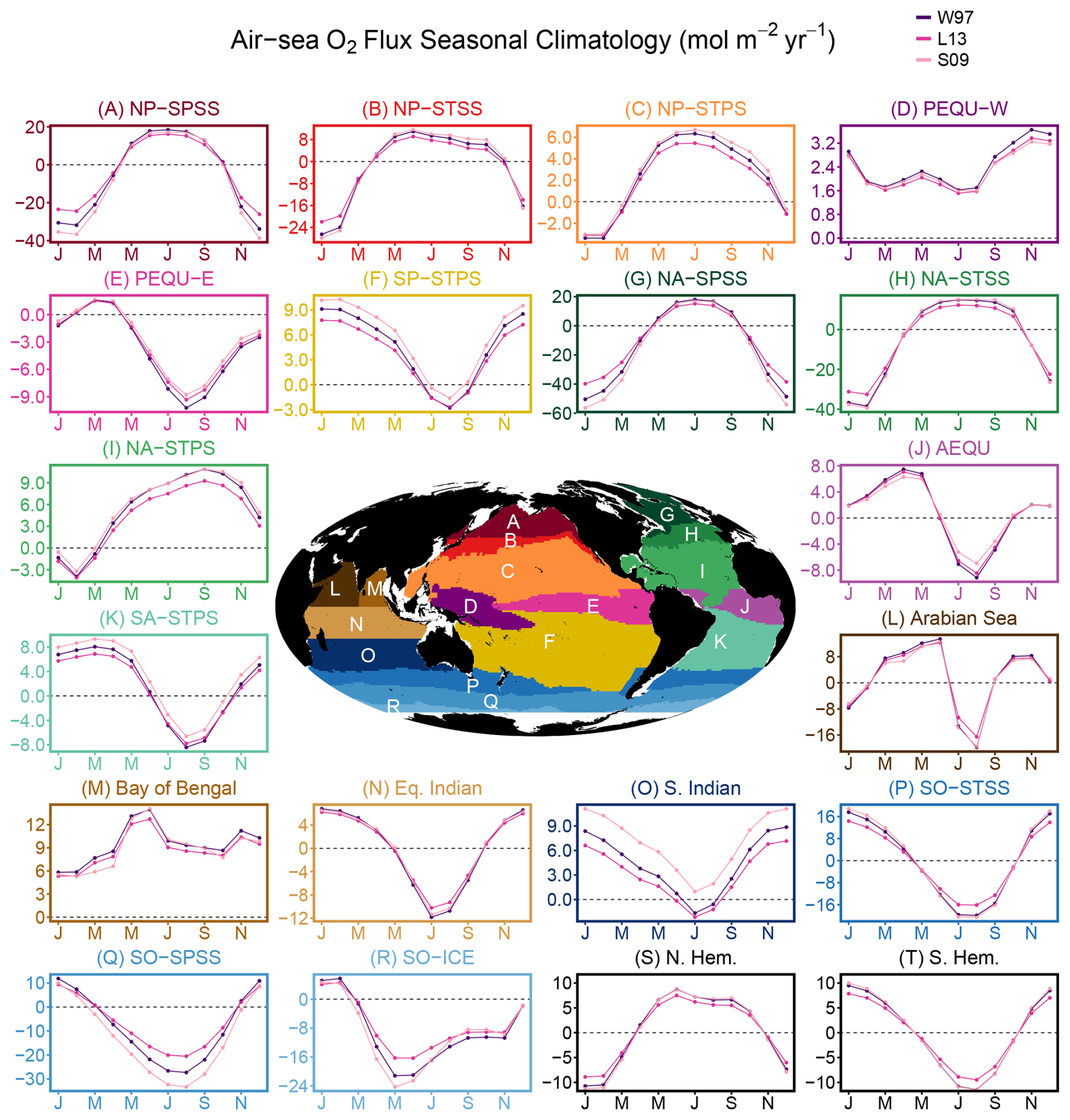
Figure A1Similar to Fig. 2, but showing comparisons of ensemble mean air-sea O2 flux seasonal climatologies for 18 RECCAP2 regions plus the two hemispheric averages resolved using each of the three gas exchange parameterization schemes (W97, L13, and S09) and the CCMP wind product.
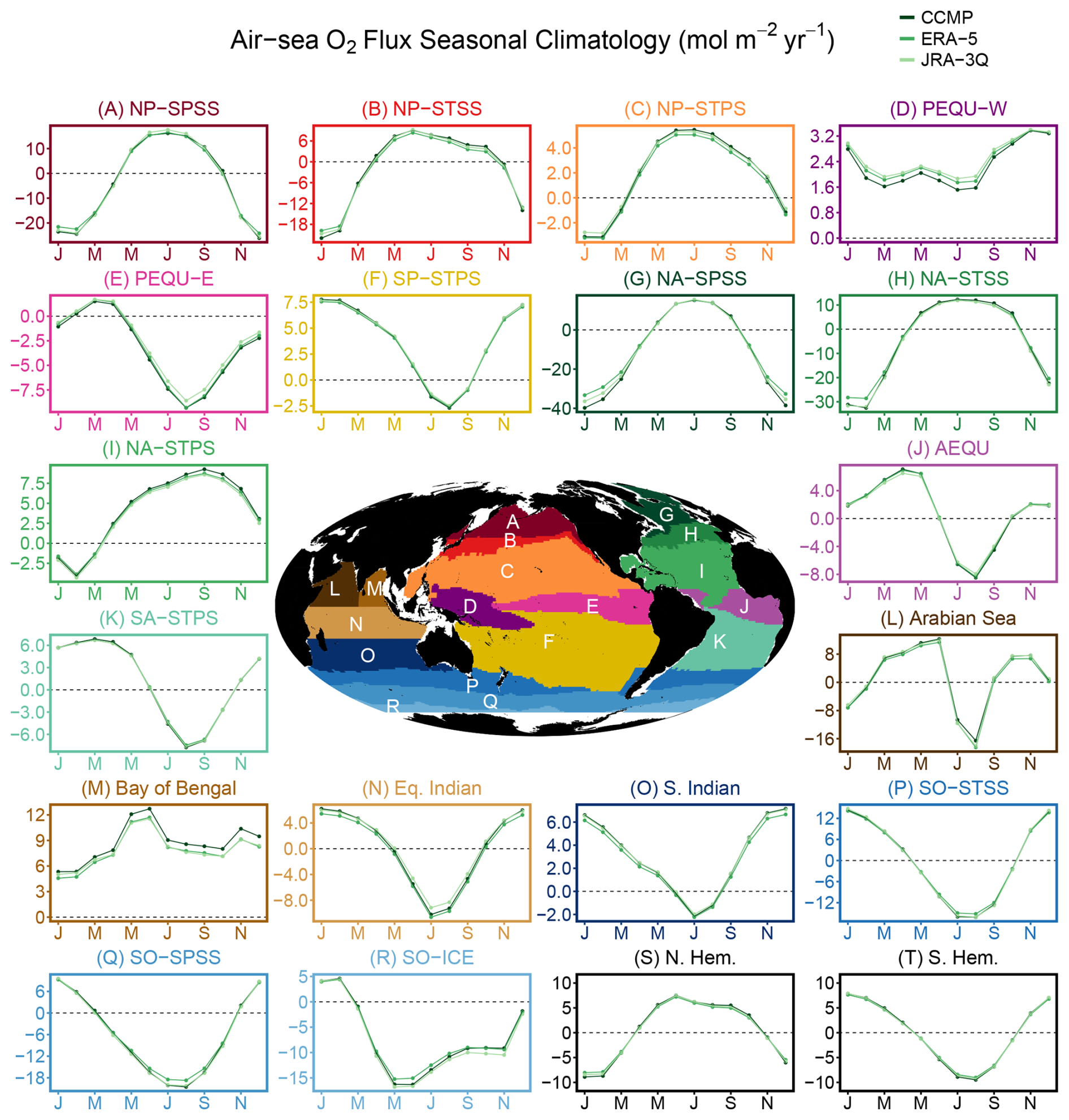
Figure A2Similar to Fig. 2, but showing comparisons of ensemble mean air-sea O2 flux seasonal climatologies for 18 RECCAP2 regions plus the two hemispheric averages resolved using each of the three wind products (CCMP, ERA5, and JRA-3Q) and the L13 gas exchange parameterization scheme.
We apply concentration adjustments to GOBAI-O2 DO fields to force global and regional annual mean fluxes to match independent observation-based estimates. For the global annual flux (), we adopt the method in Keeling and Manning (2014), following
In this equation, (4.8 ± 2.6 nmol J−1) is the O2 flux to ocean heat flux ratio (Keeling and Garcia, 2002). Q is the net observed change in ocean heat content, computed by combining the 0 to 2 km depth range from the NCEI product (Levitus et al., 2012, 2017) and below-2 km warming with a constant rate of change of 1.0 ZJ yr−1 (Desbruyères et al., 2016). ZanthN is an additional term quantifying the outgassing due to nitrogen deposition, estimated to be 19 ± 10 Tmol yr−1 (Keeling and Manning, 2014; Resplandy et al., 2019). This estimate effectively quantifies the expected annual O2 flux due to solubility effects (i.e., ocean warming) and additional influences of ocean stratification and biology averaged over interannual to decadal time scales.
We calculate for each year after 1980. However, the raw annual values exhibit IAV with substantial uncertainties, driven primarily by fluctuations in ocean heat content. The relationship between ocean heat flux and O2 flux in is more robust on decadal timescales than for IAV, as shorter-term variations in air-sea O2 exchange can be influenced by ocean ventilation that are not directly coupled to heat uptake (Hamme and Keeling, 2008; Keeling and Garcia, 2002). To reduce this IAV and provide a constraint that better reflects the near-steady state heat-O2 relationship, we calculate smoothed annual values by applying a weighted linear regression to the time series, with weights determined by the inverse square of the annual uncertainties. The uncertainty in the smoothed for each year incorporates the uncertainty in the fitted regression line itself, quantified by the standard error of the fitted values and the underlying uncertainties in the raw calculations. We combine these uncertainties in quadrature to obtain the total 1σ uncertainty for each year. For 2024, where no raw calculation exists, we use the mean raw uncertainty from 2004–2023 as a representative estimate. The linear fit yields a in 2004 of 53 ± 49.4 Tmol yr−1, and in 2024 of 70 ± 33.1 Tmol yr−1, with a 2004–2024 average value of 61 Tmol yr−1. We report the raw and fitted value as well as uncertainties in Table B1.
Table B1Global annual mean air-sea O2 flux derived from ocean heat content changes with nitrogen deposition adjustment (Eq. B1). The original flux represents yearly estimates, while the smoothed flux is obtained from an uncertainty-weighted linear regression to smooth the original flux that has large IAV. We therefore use the smoothed flux to constrain our annual mean flux estimates. Uncertainties (1σ) for the original flux incorporate errors in the O2-to-heat flux ratio, global ocean heat content changes, and the nitrogen deposition adjustment. Uncertainties for the smoothed flux are calculated as the root sum of squares of the original flux uncertainty and the regression fit uncertainty.
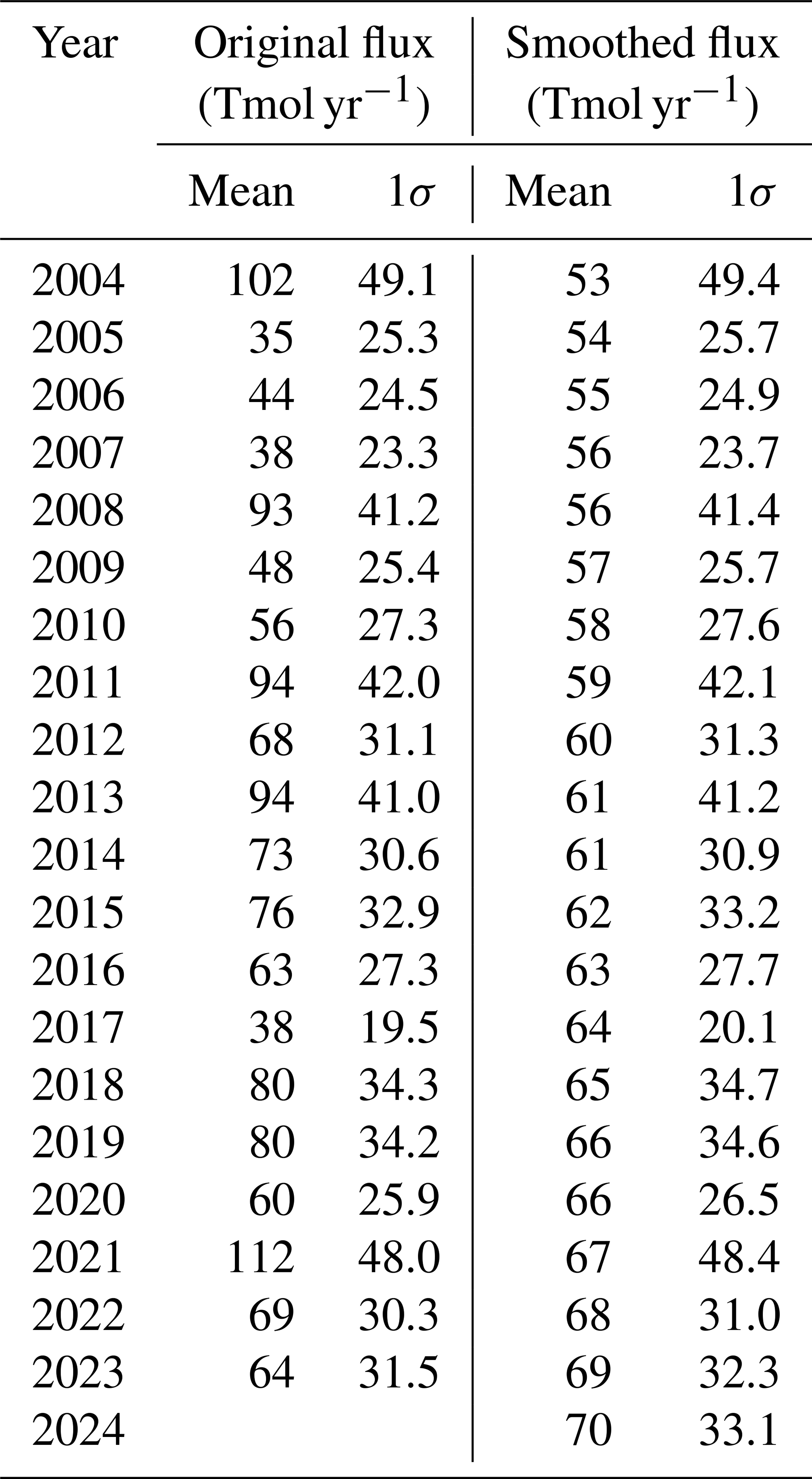
We also adjust regional annual mean fluxes to match ocean inversion model estimates of annual O2 flux from Resplandy et al. (2016), which reported fluxes for 21 ocean basins from seven inversions. We only use five of the seven inversions (Table B2) that are selected based on their smaller tropical-southern ocean O2 flux gradients with better agreement to atmospheric observations of O2 gradients. Nevertheless, the five products still overestimate the tropical-extratropical flux gradient (Fig. 8). For each inversion, we integrate the flux into six large ocean regions (Fig. B1) rather than finer spatial scales to minimize abrupt changes in flux at the regional boundaries (Table B2). These inversions represent only the pre-industrial steady state, and their regional fluxes sum to near zero globally. Because these inversions do not include regional variations in climate change impacts, our flux adjustments may not fully capture anthropogenic trends in air-sea O2 fluxes that vary spatially.
For each ensemble iteration of flux estimation and for each year, we adjust the DO field by a set of constant values for each of the six ocean regions corresponding to a randomly selected inversion from the five available for individual regions (Table B2), and a global adjustment randomly sampled from Table B1. Adjusting the regional and global total fluxes every year removes the original flux IAV and trends from the raw flux product, while imposing smoothed global annual mean flux trends derived from the ocean heat flux constraint.
The adjustment for GOBAI-O2 v2.3 (Fig. B2), averaged from 2004 to 2024, indicates that DO concentrations need to be adjusted downward in five of the six ocean regions, resulting in greater ocean O2 uptake or reduced outgassing in the adjusted flux estimates, while the Southern Ocean requires a small upward adjustment that reduces its O2 uptake. In descending order, the averaged adjustments are −1.68 µmol kg−1 for the Indian Ocean, −1.43 µmol kg−1 for the North Atlantic, −1.37 µmol kg−1 for the Equatorial Pacific, −1.32 µmol kg−1 for the Equatorial Atlantic, −1.18 µmol kg−1 for the North Pacific, and 0.58 µmol kg−1 for the Southern Ocean.
Applying a constant adjustment inside each region and a different constant in the neighbouring region produces an abrupt step in the adjusted flux boundary. We therefore smooth the regional adjustment across boundaries. For each region, we smooth its regional mask with a Gaussian kernel of 3° standard deviation truncated at 9°, so that the adjustment varies gradually across each boundary and stays constant in the interior of each region. Because each regional adjustment also acts on the neighbouring regions, the regional adjustments are solved jointly, which keeps the annual mean flux integrated over each original region equal to its inversion target. This smoothing slightly shifts the adjusted hemispheric fluxes from 75 and −14 to 71 and −13 Tmol yr−1 for the Northern and Southern Hemispheres, respectively, based on v2.3.
Over time, the adjustments show a trend toward larger reductions in DO concentrations in the Indian Ocean and Equatorial Atlantic (p< 0.05), while other regions exhibit no significant temporal trends. This pattern occurs because GOBAI-O2 v2.3 DO concentrations in these two regions decrease faster than the corresponding decline in O2 saturation calculated from temperature and salinity, which would produce an increasing trend in oceanic O2 uptake without the annual mean flux adjustment.
The adjustment pattern varies across the three GOBAI-O2 versions (Figs. S12–S13), which produce differences in mean DO over each ocean region. The required adjustments differ in both magnitude and sign among versions, with v2.1 and v2.2 requiring upward adjustments in all six regions and v2.3 requiring downward adjustments in five of the six regions. This disagreement indicates that each version carries its own systematic bias in regional mean DO, and that the bias is a leading source of uncertainty in the annual mean flux (Sect. 4.2). Among the three versions, v2.3 requires the smallest maximum regional adjustment. The adjustments remain relatively small (< 2 %) compared to annual average DO concentrations of approximately 350 µmol kg−1 in high-latitude regions and 200 µmol kg−1 in tropical oceans. The adjustments have only minimal impacts on the flux seasonal cycle (Fig. B3).
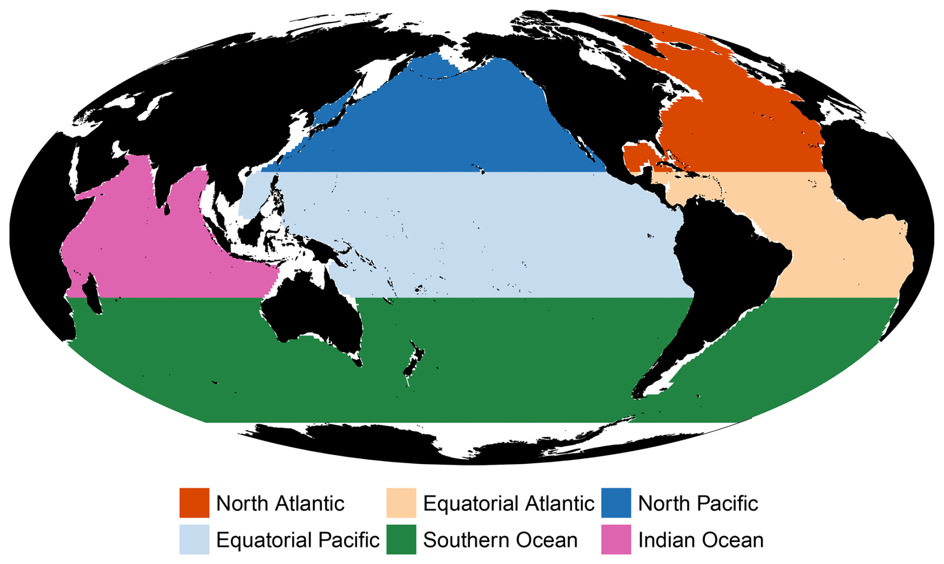
Figure B1Map of six ocean regions used to constrain annual mean fluxes through five ocean inversion estimates. Each colored region represents a distinct oceanic domain where region-specific inversion constraints are applied to adjust the calculated air-sea O2 flux annual means. For each region, the target annual mean flux is integrated from finer-scale regions reported in Resplandy et al. (2016).
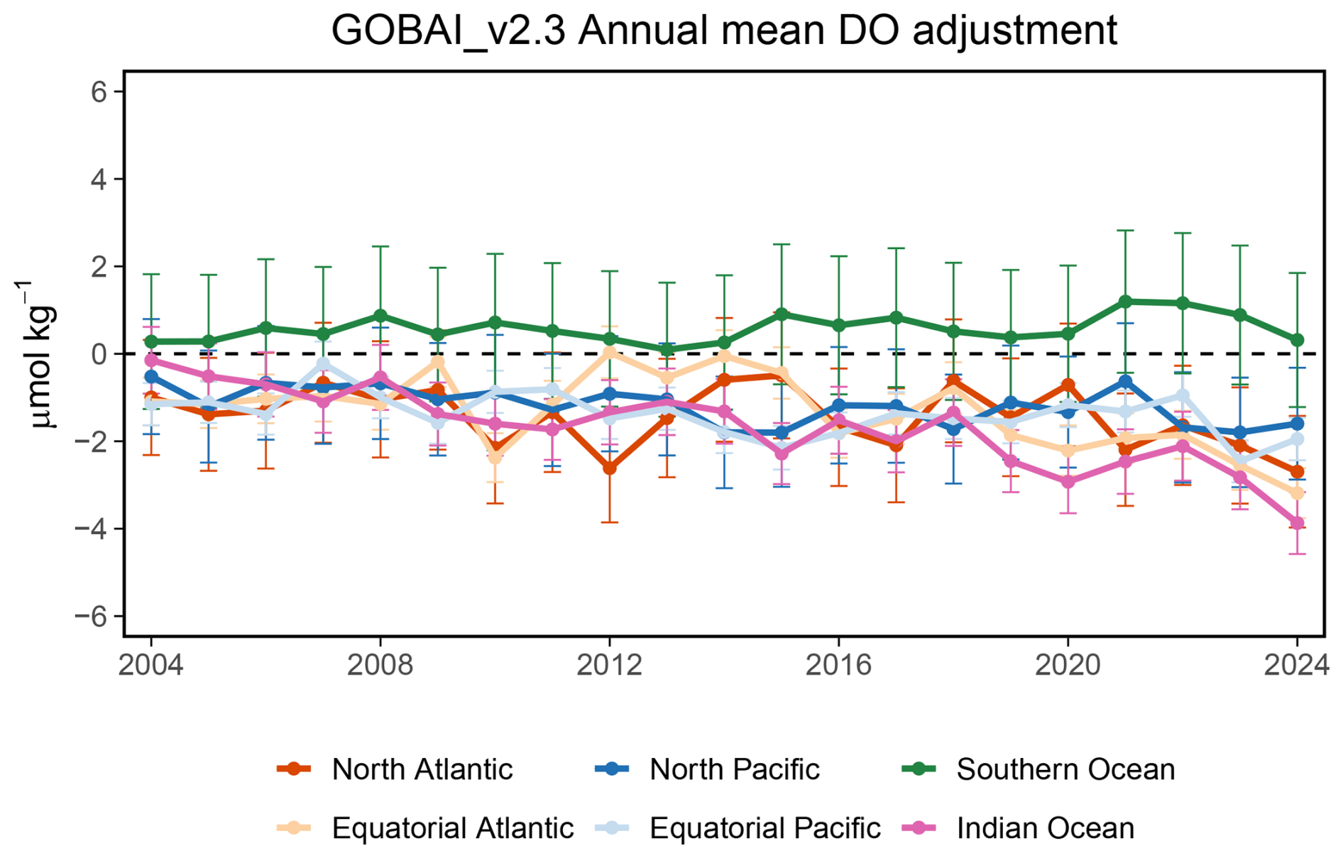
Figure B2Required annual mean DO adjustment for the six ocean regions (Fig. B1) by year, based on fluxes calculated using GOBAI-O2 v2.3. These adjustments include both the global annual mean adjustment and the regional adjustments. Similar figures showing required annual mean DO adjustments for fluxes calculated using GOBAI-O2 v2.1 and v2.2 are shown in Figs. S12–S13, which reveal significant differences compared to v2.3, highlighting the sensitivity of annual mean DO to ML methods.
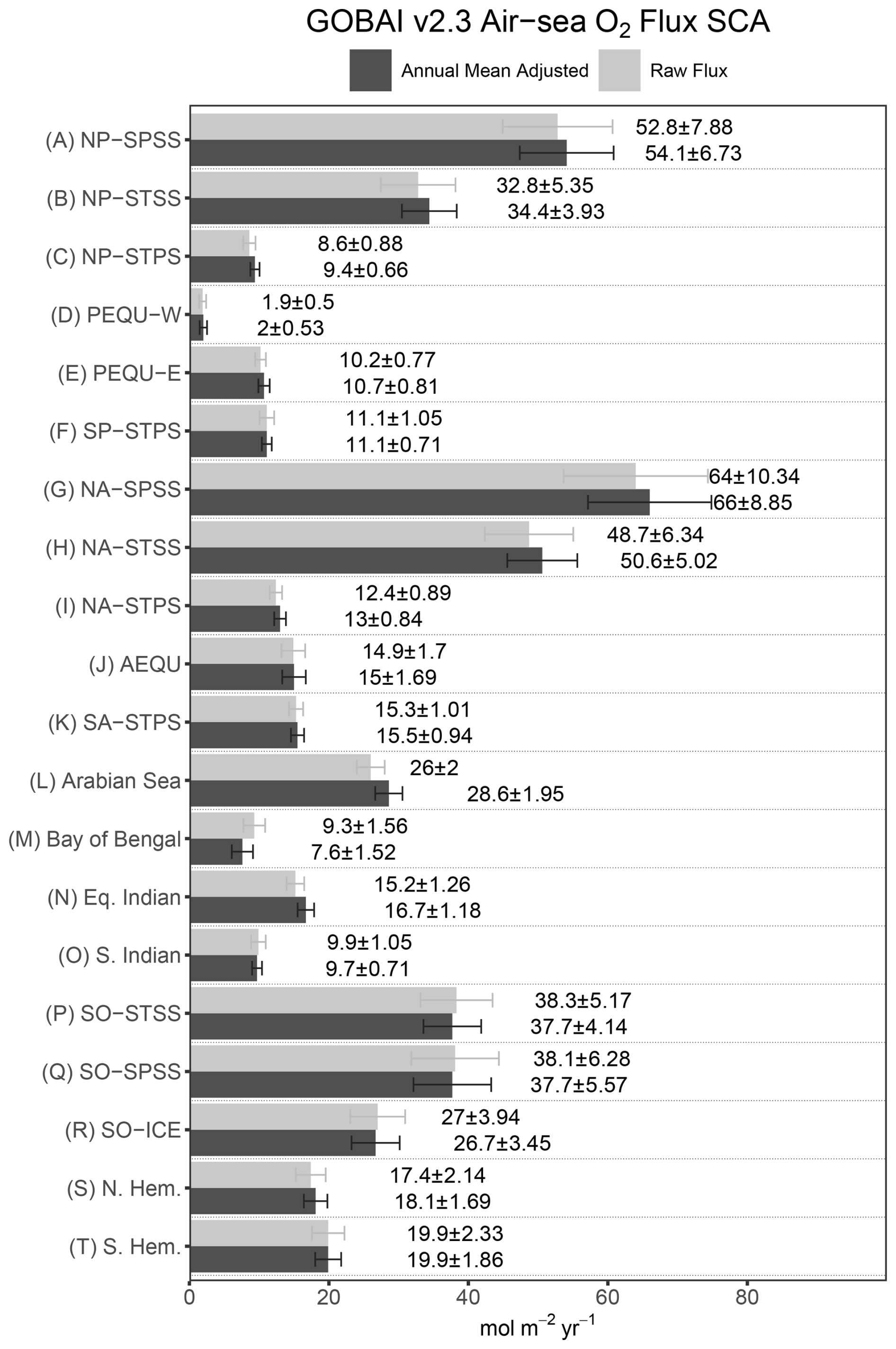
Figure B3Comparison of air-sea O2 flux SCA for 18 RECCAP2 regions plus the two hemispheric averages calculated using raw fluxes (gray) versus fluxes from annual mean-adjusted DO (black). Values are shown in mol m−2 yr−1 based on GOBAI-O2 v2.3. The ensemble 1σ standard deviation is also shown. Annual mean flux adjustments affect the flux seasonal cycle because temporally constant DO adjustments interact with seasonally varying wind speeds in the gas exchange parameterization.
Table B2Area-integrated annual mean air-sea O2 flux (Tmol) of six large regions (Fig. B1) estimated by five ocean inversions from Resplandy et al. (2016). Positive as ocean O2 outgassing.
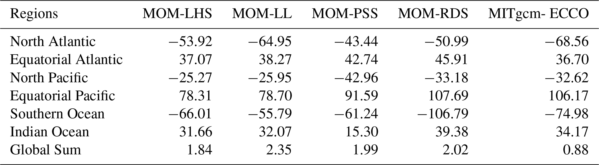
The surface station APO observations are from the Scripps O2 program (Keeling and Morgan, 2019). We use flask δ(O) and CO2 data at roughly two samples per month (Eq. 8) collected during clean background air conditions from 10 sampling sites along the Pacific (map shown in Fig. S1A). Flask samples are analyzed at Scripps using a custom interferometer and a non-dispersive infrared analyzer. The sample times match the NOAA ObsPack CO2 files from the Scripps O2 Program (Schuldt et al., 2021).
APO observations in per meg units can be broken down into contributions from air-sea O2 (), air-sea CO2 (), air-sea N2 (), fossil fuel O2 (), and fossil fuel CO2 () fluxes, following
where (0.2094) and (0.7808) are the dry-air mole fractions of O2 and N2 in the atmosphere, and Δ represents deviation in the atmospheric concentration of a tracer in units of ppm created by the corresponding fluxes. The value of is the reference mole fraction of the Scripps O2 Program scale (Keeling and Morgan, 2019), a defined constant of the measurement scale corresponding to an estimate of the atmospheric composition in the mid 1980s derived from Machta and Hughes (1970). Dividing by or converts the unit from ppm-equivalent to per meg. For each tracer component on the RHS of Eq. (C1), except , which is our target, we use model forward transport of flux fields sampled at measurement locations and times. For each tracer, we employ two different flux products and four different transport models from the APO forward transport model intercomparison project (APO-MIP1, Jin et al., 2025). The sum of the last two terms in Eq. (C1) forms ΔAPOff, which represents APO changes due to fossil fuel burning.
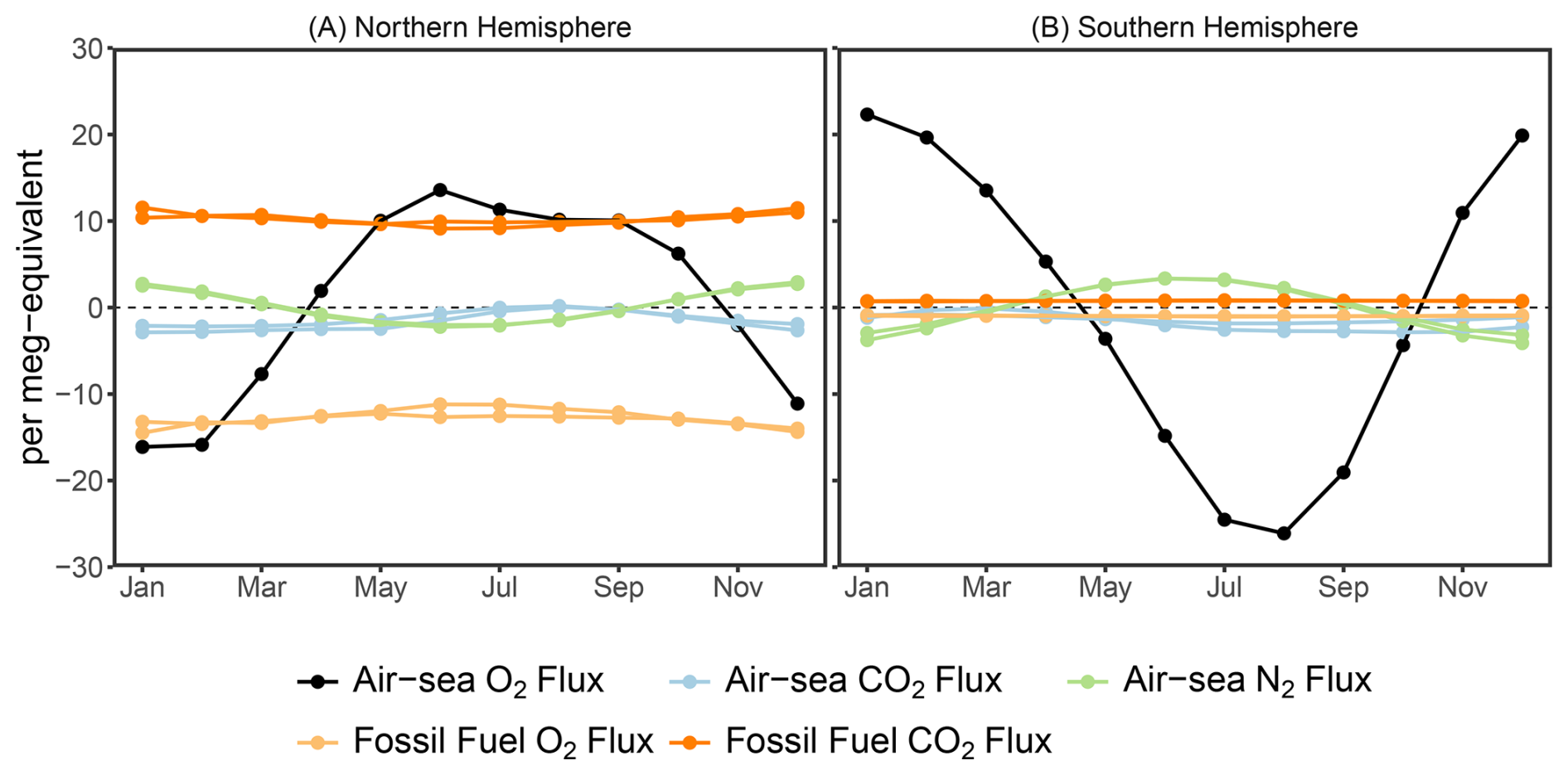
Figure C1Monthly climatology (2004–2024) of hemispheric mean air-sea O2 flux from this study (black), averaged across the flux ensemble (Sect. 2.5), compared to non-oceanic flux correction components (2004–2020 average) used to correct APO observations. Each flux type for correction is shown for the two flux products described in Appendix C, with both products of a given type sharing the same color, so eight colored curves are plotted in each panel. We note that the two air-sea N2 flux products essentially overlap, and the two fossil fuel O2 and the two fossil fuel CO2 flux products largely overlap, reflecting the consistency of these flux fields between products. Each flux component (Tmol d−1) creates an atmospheric tracer concentration in ppm units, which can be further converted to per meg units through scaling (Eq. C1). Here, we scale each flux component to directly show its contribution to observed APO in the per meg-equivalent unit. Note that air-sea N2 flux is sign-reversed according to Eq. (C1). The comparison demonstrates that the non-oceanic O2 flux components have much smaller seasonal variations compared to the dominant air-sea O2 flux that drives the observed APO seasonal cycle.
For , we use a configuration of the Community Earth System Model (CESM2) Forced Ocean-Sea-Ice (FOSI) simulation (Yeager et al., 2022) and a ML interpolation of pCO2 based air-sea CO2 fluxes (Jersild et al., 2017; Landschützer et al., 2016).
For , we use two flux products () derived by scaling ocean heat flux from ERA5 reanalyses (Hersbach et al., 2020) and CESM2, following
where (mol kg−1 °C−1) is the temperature derivative of solubility using solubility coefficients from Hamme and Emerson (2004). Cp represents the specific heat capacity of seawater, which is assumed to be 3993 J kg−1 °C−1. The factor of is to adjust the seasonal amplitude as proposed by Jin et al. (2007).
For and , we use fossil CO2 emission and O2 uptake fluxes from Jones et al. (2021), and CO2 emission as prepared for the OCO-2 Model Intercomparison Project (MIP) version 10, downloaded from Basu and Nassar (2021). For the second product, O2 combustion is not available, but we estimate by scaling the atmospheric field of by a factor of −1.4 (Keeling, 1988; Steinbach et al., 2011).
We use four transport models. These include two versions of NICAM-TM, based on the Nonhydrostatic Icosahedral Atmospheric Model (NICAM) (Niwa et al., 2011; Satoh et al., 2014); MIROC4-ACTM, a new generation Model for Interdisciplinary Research on Climate (MIROC, version 4.0; Watanabe et al., 2008); the atmospheric general circulation model (AGCM)-based chemistry-transport model (ACTM; Patra et al., 2018); and the Community Atmosphere Model with specified dynamics (CAM-SD), which is the atmospheric component of CESM2 (Danabasoglu et al., 2020). Detailed descriptions of these models are available in Jin et al. (2025).
We use airborne APO data from the NSF NCAR GV aircraft during the HIAPER Pole-to-Pole Observations (HIPPO, Wofsy, 2011) project from 2009–2011, the O Ratio and CO2 Airborne Southern Ocean Study (ORCAS, Stephens et al., 2018) in January and February of 2016, and the NASA DC-8 aircraft during the Atmospheric Tomography Mission (ATom, Thompson et al., 2022) from 2016 to 2018. HIPPO consisted of five campaigns along a Pacific transect, ATom consisted of four campaigns covering both Pacific and Atlantic transects, and the six-week ORCAS campaign provided dense sampling over the Drake Passage and ocean areas adjacent to the tip of South America and the Antarctic Peninsula. The horizontal flight tracks are shown in Fig. S1B–D.
Airborne APO measurements were made with the NSF NCAR Airborne Oxygen Instrument (AO2), using a vacuum-ultraviolet absorption technique to measure O2 and a single-cell infrared gas analyzer to measure CO2 (Stephens et al., 2021g). AO2 produces measurements every 2.5 s, which are averaged to 10 s frequency for merging with other aircraft data. Airborne data are also selected to match with the ObsPack CO2 files. The AO2 measurements were adjusted on a per flight basis to agree with air samples collected during flight by the NSF NCAR/Scripps Medusa flask sampler, which captures 32 samples per flight for subsequent laboratory analysis at Scripps (Bent, 2014; Stephens et al., 2021g). These flask samples help identify and correct time-dependent systematic biases in the continuous measurements. Before being used as a reference, the Medusa data underwent their own adjustment process to minimize diffusive fractionation effects inherent in flask sampling by applying an correction following
where δ(O)obs and represent Medusa flask measurements (Stephens et al., 2021g). The coefficient 3.77 represents the theoretical ratio between ) and δ(O) variations resulting from thermal fractionation processes (Keeling et al., 2004; Stephens et al., 2021g), and is applied consistently across all campaigns. The constant 15 per meg is the approximate global surface mean value from the Scripps stations on the Scripps scale. The corrected δ(O)* has reduced sensitivity to both thermal and pressure-gradient fractionation artifacts arising from airborne sampling and laboratory analysis.
Therefore, our AO2 APO measurements adjusted to match Medusa data are effectively APO* that contains ), following
The ) adjustment has minimal impact on the APO annual mean value, but it scales down the APO seasonal cycle amplitude by about 4 % (Jin et al., 2025). We correct for this ) component of APO* by including an extra correction, which is scaled from the correction (Jin et al., 2023), following
where XAr (0.00934) is the mole fraction of Ar in the atmosphere. is a scaling factor, which is the ratio of Ar and N2 air-sea fluxes driven by heat flux from Table 3 in Manizza et al. (2012).
Therefore, to correct for the non-oceanic O2 flux contribution in airborne APO* data, we adapt Eq. (C1) following
using the same fluxes and forward atmospheric transport as described above. To quantify the uncertainty of , we generate a large ensemble of station and airborne . We first generate a large ensemble (1000 members) of observation data. For airborne APO* data, we consider uncertainty due to measurement imprecision and reproducibility (Stephens et al., 2021g), and the uncertainty of the land biosphere O2:CO2 exchange ratio. For station APO data, we generate a large ensemble of measurements using an error model that considers a span error of 1% in the laboratory calibration scale (Keeling et al., 2020) and long-term reference cylinder effects including corrosion error of ±0.3 per meg yr−1, leakage error of ±0.2 per meg yr−1, and desorption error of ±0.1 per meg yr−1 (Keeling et al., 2007). These systematic errors are held constant across all stations for each ensemble member. In addition, for each individual flask measurement, we add a random analytical error of ±3.3 per meg and a thermal fractionation error of ±2 per meg. Using two air-sea CO2 flux products, two air-sea N2 flux products, two fossil fuel O2 and CO2 flux products, and four atmospheric transport models, we generate 32 unique non-oceanic O2 flux correction combinations. We apply each combination to the station APO or airborne APO* large ensemble, leading to 32 000 estimates of . The uncertainty of the seasonal cycle and annual mean value at each station and for the latitudinally-binned airborne tropospheric-average is then calculated as the 1σ ensemble spread. We note that these non-oceanic O2 flux corrections have a small impact on the APO seasonal cycle (Fig. C1), but that the annual mean component of APO is particularly sensitive to the air-sea CO2 flux and fossil fuel O2 and CO2 fluxes (Fig. 7). For this reason, and because our atmospheric transport model simulations have arbitrary background concentrations, we cannot compare the global annual-mean observed to forward transport simulations of our flux product. Thus, the meridional tropospheric-average gradient comparison shown in Fig. 8 includes an arbitrary global-mean adjustment that sets global mean concentrations to zero.
The supplement related to this article is available online at https://doi.org/10.5194/essd-18-8407-2026-supplement.
YJ conceived of the project, conducted the analysis, generated the data products and figures, and wrote the paper. EM and BS provided atmospheric O2 measurements. JS provided the GOBAI-O2 product. All authors contributed to reviewing and editing the text.
The contact author has declared that none of the authors has any competing interests.
Publisher's note: Copernicus Publications remains neutral with regard to jurisdictional claims made in the text, published maps, institutional affiliations, or any other geographical representation in this paper. The authors bear the ultimate responsibility for providing appropriate place names. Views expressed in the text are those of the authors and do not necessarily reflect the views of the publisher.
Atmospheric O2 measurements on HIPPO were supported by NSF grants ATM-0628519 and ATM-0628388. ORCAS was supported by NSF grants PLR-1501993, PLR-1502301, PLR-1501997, and PLR-1501292. Atmospheric O2 measurements on ATom 1 were supported by NSF grants AGS-1547626 and AGS-1547797. Atmospheric O2 measurements on ATom 2-4 were supported by NSF grants AGS-1623745 and AGS-1623748. The recent atmospheric measurements of the Scripps O2 program have been supported via funding from the NSF and the National Oceanic and Atmospheric Administration (NOAA) under Grants OPP-1922922, OPP-2329254, and NA20OAR4320278, respectively. We acknowledge atmospheric transport modelers, including Jesse Vance and Matthew Long (CAM-SD), Yosuke Niwa (NICAM), and Prabir K. Patra (MIROC4-ACTM), for providing atmospheric simulations of APO components. Y.J. would like to acknowledge the Advanced Study Program Postdoctoral Fellowship of the NSF National Center for Atmospheric Research. We thank Raymond Najjar and an anonymous reviewer for their constructive comments that improved the manuscript.
This material is based upon work supported by the NSF National Center for Atmospheric Research, which is a major facility sponsored by the U.S. National Science Foundation under Cooperative Agreement No. 1852977. M.M. acknowledges support from NASA (IDS-#190113), NSF (OCE-2049294), and the National Recovery and Resilience Plan project TeRABIT (Terabit network for Research and Academic Big data in Italy – IR0000022 – PNRR Missione 4, Componente 2, Investimento 3.1 CUP I53C21000370006) in the frame of the European Union – NextGenerationEU funding. The development of GOBAI-O2 and the work of J.S. have been supported by the Cooperative Institute for Climate, Ocean, & Ecosystem Studies at the University of Washington under NOAA cooperative agreement NA20OAR4320271 (CICOES contribution no. 2025-1503), by NOAA's Pacific Marine Environmental Laboratory (PMEL contribution no. 5959), and by NOAA's National Marine Fisheries Service under the Essential Data Acquisition efforts of the Inflation Reduction Act via award NA24NMFX405C0016-T1-01.
This paper was edited by Sabine Schmidt and reviewed by Raymond Najjar and one anonymous referee.
Atamanchuk, D., Koelling, J., Send, U., and Wallace, D. W. R.: Rapid transfer of oxygen to the deep ocean mediated by bubbles, Nat. Geosci., 13, 232–237, https://doi.org/10.1038/s41561-020-0532-2, 2020.
Banerjee, P. and Kumar, P. S.: Dust-induced episodic phytoplankton blooms in the Arabian Sea during winter monsoon, J. Geophys. Res.-Oceans, 119, 7123–7138, https://doi.org/10.1002/2014JC010304, 2014.
Basu, S. and Nassar, R.: Fossil Fuel CO2 Emissions for the OCO2 Model Intercomparison Project (MIP) (2020.1), Zenodo [data set], https://doi.org/10.5281/zenodo.4776925, 2021.
Bates, D., Mächler, M., Bolker, B., and Walker, S.: Fitting Linear Mixed-Effects Models Using lme4, J. Stat. Softw., 67, https://doi.org/10.18637/jss.v067.i01, 2015.
Battle, M., Fletcher, S. M., Bender, M. L., Keeling, R. F., Manning, A. C., Gruber, N., Tans, P. P., Hendricks, M. B., Ho, D. T., Simonds, C., Mika, R., and Paplawsky, B.: Atmospheric potential oxygen: New observations and their implications for some atmospheric and oceanic models, Global Biogeochem. Cy., 20, GB1010, https://doi.org/10.1029/2005GB002534, 2006.
Behrenfeld, M. J., Boss, E., Siegel, D. A., and Shea, D. M.: Carbon-based ocean productivity and phytoplankton physiology from space, Global Biogeochem. Cy., 19, GB1006, https://doi.org/10.1029/2004GB002299, 2005.
Bender, M. L., Ho, D. T., Hendricks, M. B., Mika, R., Battle, M. O., Tans, P. P., Conway, T. J., Sturtevant, B., and Cassar, N.: Atmospheric O changes, 1993–2002: Implications for the partitioning of fossil fuel CO2 sequestration, Global Biogeochem. Cy., 19, GB4017, https://doi.org/10.1029/2004GB002410, 2005.
Bent, J.: Airborne Oxygen Measurements over the Southern Ocean as an Integrated Constraint of Seasonal Biogeochemical Processes, PhD thesis, University of California, San Diego, https://escholarship.org/uc/item/4dd6k6j2 (last access: 4 November 2026), 2014.
Bittig, H., Wong, A., and Plant, J.: BGC-Argo synthetic profile file processing and format on Coriolis GDAC, Version 1.3, Ifremer, https://doi.org/10.13155/55637, 2022.
Bolton, D.: The Computation of Equivalent Potential Temperature, Mon. Weather Rev., 108, 1046–1053, https://doi.org/10.1175/1520-0493(1980)108<1046:TCOEPT>2.0.CO;2, 1980.
Boyer, T., Conkright, M. E., and Levitus, S.: Seasonal variability of dissolved oxygen, percent oxygen saturation, and apparent oxygen utilization in the Atlantic and Pacific Oceans, Deep-Sea Res., 46, 1593–1663, https://doi.org/10.1016/S0967-0637(99)00021-7, 1999.
Brandt, P., Alory, G., Awo, F. M., Dengler, M., Djakouré, S., Imbol Koungue, R. A., Jouanno, J., Körner, M., Roch, M., and Rouault, M.: Physical processes and biological productivity in the upwelling regions of the tropical Atlantic, Ocean Sci., 19, 581–601, https://doi.org/10.5194/os-19-581-2023, 2023.
Breitburg, D., Levin, L. A., Oschlies, A., Grégoire, M., Chavez, F. P., Conley, D. J., Garçon, V., Gilbert, D., Gutiérrez, D., Isensee, K., Jacinto, G. S., Limburg, K. E., Montes, I., Naqvi, S. W. A., Pitcher, G. C., Rabalais, N. N., Roman, M. R., Rose, K. A., Seibel, B. A., Telszewski, M., Yasuhara, M., and Zhang, J.: Declining oxygen in the global ocean and coastal waters, Science, 359, https://doi.org/10.1126/science.aam7240, 2018.
Busecke, J. J. M., Resplandy, L., Ditkovsky, S. J., and John, J. G.: Diverging Fates of the Pacific Ocean Oxygen Minimum Zone and Its Core in a Warming World, AGU Adv., 3, e2021AV000470, https://doi.org/10.1029/2021AV000470, 2022.
Bushinsky, S. M. and Emerson, S. R.: Biological and physical controls on the oxygen cycle in the Kuroshio Extension from an array of profiling floats, Deep-Sea Res., 141, 51–70, https://doi.org/10.1016/j.dsr.2018.09.005, 2018.
Bushinsky, S. M., Gray, A. R., Johnson, K. S., and Sarmiento, J. L.: Oxygen in the Southern Ocean from Argo floats: Determination of processes driving air-sea fluxes, J. Geophys. Res.-Oceans, 122, 8661–8682, https://doi.org/10.1002/2017JC012923, 2017.
Bushinsky, S. M., Nachod, Z., Fassbender, A. J., Tamsitt, V., Takeshita, Y., and Williams, N.: Offset Between Profiling Float and Shipboard Oxygen Observations at Depth Imparts Bias on Float pH and Derived pCO2, Global Biogeochem. Cy., 39, e2024GB008185, https://doi.org/10.1029/2024GB008185, 2025.
Cheng, L., Trenberth, K. E., Fasullo, J., Boyer, T., Abraham, J., and Zhu, J.: Improved estimates of ocean heat content from 1960 to 2015, Sci. Adv., 3, https://doi.org/10.1126/sciadv.1601545, 2017.
Danabasoglu, G., Lamarque, J.-F., Bacmeister, J., Bailey, D. A., DuVivier, A. K., Edwards, J., Emmons, L. K., Fasullo, J., Garcia, R., Gettelman, A., Hannay, C., Holland, M. M., Large, W. G., Lauritzen, P. H., Lawrence, D. M., Lenaerts, J. T. M., Lindsay, K., Lipscomb, W. H., Mills, M. J., Neale, R., Oleson, K. W., Otto-Bliesner, B., Phillips, A. S., Sacks, W., Tilmes, S., van Kampenhout, L., Vertenstein, M., Bertini, A., Dennis, J., Deser, C., Fischer, C., Fox-Kemper, B., Kay, J. E., Kinnison, D., Kushner, P. J., Larson, V. E., Long, M. C., Mickelson, S., Moore, J. K., Nienhouse, E., Polvani, L., Rasch, P. J., and Strand, W. G.: The Community Earth System Model Version 2 (CESM2), J. Adv. Model. Earth Sy., 12, e2019MS001916, https://doi.org/10.1029/2019MS001916, 2020.
De Boyer Montégut, C., Madec, G., Fischer, A. S., Lazar, A., and Iudicone, D.: Mixed layer depth over the global ocean: An examination of profile data and a profile-based climatology, J. Geophys. Res.-Oceans, 109, C12003, https://doi.org/10.1029/2004JC002378, 2004.
Deike, L., Zhou, X., Rustogi, P., Stanley, R. H. R., Reichl, B. G., Bushinsky, S. M., and Resplandy, L.: A universal wind–wave–bubble formulation for air–sea gas exchange and its impact on oxygen fluxes, P. Natl. Acad. Sci. USA, 122, e2419319122, https://doi.org/10.1073/pnas.2419319122, 2025.
Desbruyères, D. G., Purkey, S. G., McDonagh, E. L., Johnson, G. C., and King, B. A.: Deep and abyssal ocean warming from 35 years of repeat hydrography, Geophys. Res. Lett., 43, 10356–10365, https://doi.org/10.1002/2016GL070413, 2016.
Donlon, C. J., Minnett, P. J., Gentemann, C., Nightingale, T. J., Barton, I. J., Ward, B., and Murray, M. J.: Toward Improved Validation of Satellite Sea Surface Skin Temperature Measurements for Climate Research, J. Climate, 15, 353–369, https://doi.org/10.1175/1520-0442(2002)015<0353:TIVOSS>2.0.CO;2, 2002.
Eddebbar, Y. A., Long, M. C., Resplandy, L., Rödenbeck, C., Rodgers, K. B., Manizza, M., and Keeling, R. F.: Impacts of ENSO on air-sea oxygen exchange: Observations and mechanisms, Global Biogeochem. Cy., 31, 901–921, https://doi.org/10.1002/2017GB005630, 2017.
Emerson, S.: Seasonal oxygen cycles and biological new production in surface waters of the subarctic Pacific Ocean, J. Geophys. Res.-Oceans, 92, 6535–6544, https://doi.org/10.1029/JC092iC06p06535, 1987.
Emerson, S. and Bushinsky, S.: The role of bubbles during air-sea gas exchange, J. Geophys. Res.-Oceans, 121, 4360–4376, https://doi.org/10.1002/2016JC011744, 2016.
Fay, A. R., Gregor, L., Landschützer, P., McKinley, G. A., Gruber, N., Gehlen, M., Iida, Y., Laruelle, G. G., Rödenbeck, C., Roobaert, A., and Zeng, J.: SeaFlux: harmonization of air–sea CO2 fluxes from surface pCO2 data products using a standardized approach, Earth Syst. Sci. Data, 13, 4693–4710, https://doi.org/10.5194/essd-13-4693-2021, 2021.
Fine, R. A., Lukas, R., Bingham, F. M., Warner, M. J., and Gammon, R. H.: The western equatorial Pacific: A water mass crossroads, J. Geophys. Res.-Oceans, 99, 25063–25080, https://doi.org/10.1029/94JC02277, 1994.
Friedlingstein, P., O'Sullivan, M., Jones, M. W., Andrew, R. M., Hauck, J., Landschützer, P., Le Quéré, C., Li, H., Luijkx, I. T., Olsen, A., Peters, G. P., Peters, W., Pongratz, J., Schwingshackl, C., Sitch, S., Canadell, J. G., Ciais, P., Jackson, R. B., Alin, S. R., Arneth, A., Arora, V., Bates, N. R., Becker, M., Bellouin, N., Berghoff, C. F., Bittig, H. C., Bopp, L., Cadule, P., Campbell, K., Chamberlain, M. A., Chandra, N., Chevallier, F., Chini, L. P., Colligan, T., Decayeux, J., Djeutchouang, L. M., Dou, X., Duran Rojas, C., Enyo, K., Evans, W., Fay, A. R., Feely, R. A., Ford, D. J., Foster, A., Gasser, T., Gehlen, M., Gkritzalis, T., Grassi, G., Gregor, L., Gruber, N., Gürses, Ö., Harris, I., Hefner, M., Heinke, J., Hurtt, G. C., Iida, Y., Ilyina, T., Jacobson, A. R., Jain, A. K., Jarníková, T., Jersild, A., Jiang, F., Jin, Z., Kato, E., Keeling, R. F., Klein Goldewijk, K., Knauer, J., Korsbakken, J. I., Lan, X., Lauvset, S. K., Lefèvre, N., Liu, Z., Liu, J., Ma, L., Maksyutov, S., Marland, G., Mayot, N., McGuire, P. C., Metzl, N., Monacci, N. M., Morgan, E. J., Nakaoka, S.-I., Neill, C., Niwa, Y., Nützel, T., Olivier, L., Ono, T., Palmer, P. I., Pierrot, D., Qin, Z., Resplandy, L., Roobaert, A., Rosan, T. M., Rödenbeck, C., Schwinger, J., Smallman, T. L., Smith, S. M., Sospedra-Alfonso, R., Steinhoff, T., Sun, Q., Sutton, A. J., Séférian, R., Takao, S., Tatebe, H., Tian, H., Tilbrook, B., Torres, O., Tourigny, E., Tsujino, H., Tubiello, F., van der Werf, G., Wanninkhof, R., Wang, X., Yang, D., Yang, X., Yu, Z., Yuan, W., Yue, X., Zaehle, S., Zeng, N., and Zeng, J.: Global Carbon Budget 2024, Earth Syst. Sci. Data, 17, 965–1039, https://doi.org/10.5194/essd-17-965-2025, 2025.
Garcia, H. E. and Gordon, L. I.: Oxygen solubility in seawater: Better fitting equations, Limnol. Oceanogr., 37, 1307–1312, https://doi.org/10.4319/lo.1992.37.6.1307, 1992.
Garcia, H. E. and Keeling, R. F.: On the global oxygen anomaly and air-sea flux, J. Geophys. Res.-Oceans, 106, 31155–31166, https://doi.org/10.1029/1999JC000200, 2001.
Garcia, H. E., Wang, Z., Bouchard, C., Cross, S. L., Paver, C. R., Reagan, J. R., Boyer, T. P., Locarnini, R. A., Mishonov, A. V., Baranova, O. K., Seidov, D., and Dukhovskoy, D.: World Ocean Atlas 2023, Volume 3: Dissolved Oxygen, Apparent Oxygen Utilization, Dissolved Oxygen Saturation and 30-year Climate Normal, NOAA Atlas NESDIS 91, https://doi.org/10.25923/rb67-ns53, 2024.
Good, S. A., Martin, M. J., and Rayner, N. A.: EN4: Quality controlled ocean temperature and salinity profiles and monthly objective analyses with uncertainty estimates, J. Geophys. Res.-Oceans, 118, 6704–6716, https://doi.org/10.1002/2013JC009067, 2013.
Gouretski, V., Cheng, L., Du, J., Xing, X., Chai, F., and Tan, Z.: A consistent ocean oxygen profile dataset with new quality control and bias assessment, Earth Syst. Sci. Data, 16, 5503–5530, https://doi.org/10.5194/essd-16-5503-2024, 2024.
Gruber, N., Gloor, M., Fan, S., and Sarmiento, J. L.: Air-sea flux of oxygen estimated from bulk data: Implications For the marine and atmospheric oxygen cycles, Global Biogeochem. Cy., 15, 783–803, https://doi.org/10.1029/2000GB001302, 2001.
Hamme, R. C. and Emerson, S. R.: The solubility of neon, nitrogen and argon in distilled water and seawater, Deep-Sea Res., 51, 1517–1528, https://doi.org/10.1016/j.dsr.2004.06.009, 2004.
Hamme, R. C. and Keeling, R. F.: Ocean ventilation as a driver of interannual variability in atmospheric potential oxygen, Tellus B, 60, 706–717, https://doi.org/10.1111/j.1600-0889.2008.00376.x, 2008.
Hayward, T. L.: The shallow oxygen maximum layer and primary production, Deep-Sea Res., 41, 559–574, https://doi.org/10.1016/0967-0637(94)90095-7, 1994.
Heimann, M. and Körner, S.: The global atmospheric tracer model TM3: Model description and user's manual Release 3.8a, Max Planck Institute for Biogeochemistry, Jena, Germany, https://www.db-thueringen.de/servlets/MCRFileNodeServlet/dbt_derivate_00020679/tech_report5.pdf (last access: 4 November2026), 2003.
Herrmann, M., Najjar, R. G., Kemp, W. M., Alexander, R. B., Boyer, E. W., Cai, W.-J., Griffith, P. C., Kroeger, K. D., McCallister, S. L., and Smith, R. A.: Net ecosystem production and organic carbon balance of U.S. East Coast estuaries: A synthesis approach, Global Biogeochem. Cy., 29, 96–111, https://doi.org/10.1002/2013GB004736, 2015.
Hersbach, H., Bell, B., Berrisford, P., Hirahara, S., Horányi, A., Muñoz-Sabater, J., Nicolas, J., Peubey, C., Radu, R., Schepers, D., Simmons, A., Soci, C., Abdalla, S., Abellan, X., Balsamo, G., Bechtold, P., Biavati, G., Bidlot, J., Bonavita, M., De Chiara, G., Dahlgren, P., Dee, D., Diamantakis, M., Dragani, R., Flemming, J., Forbes, R., Fuentes, M., Geer, A., Haimberger, L., Healy, S., Hogan, R. J., Hólm, E., Janisková, M., Keeley, S., Laloyaux, P., Lopez, P., Lupu, C., Radnoti, G., de Rosnay, P., Rozum, I., Vamborg, F., Villaume, S., and Thépaut, J.-N.: The ERA5 global reanalysis, Q. J. Roy. Meteor. Soc., 146, 1999–2049, https://doi.org/10.1002/qj.3803, 2020.
Hintsa, E. J., Moore, F. L., Hurst, D. F., Dutton, G. S., Hall, B. D., Nance, J. D., Miller, B. R., Montzka, S. A., Wolton, L. P., McClure-Begley, A., Elkins, J. W., Hall, E. G., Jordan, A. F., Rollins, A. W., Thornberry, T. D., Watts, L. A., Thompson, C. R., Peischl, J., Bourgeois, I., Ryerson, T. B., Daube, B. C., Gonzalez Ramos, Y., Commane, R., Santoni, G. W., Pittman, J. V., Wofsy, S. C., Kort, E., Diskin, G. S., and Bui, T. P.: UAS Chromatograph for Atmospheric Trace Species (UCATS) – a versatile instrument for trace gas measurements on airborne platforms, Atmos. Meas. Tech., 14, 6795–6819, https://doi.org/10.5194/amt-14-6795-2021, 2021.
Huang, S., Shao, J., Chen, Y., Qi, J., Wu, S., Zhang, F., He, X., and Du, Z.: Reconstruction of dissolved oxygen in the Indian Ocean from 1980 to 2019 based on machine learning techniques, Front. Mar. Sci., 10, https://doi.org/10.3389/fmars.2023.1291232, 2023.
Ishidoya, S., Uchida, H., Sasano, D., Kosugi, N., Taguchi, S., Ishii, M., Morimoto, S., Tohjima, Y., Nishino, S., Murayama, S., Aoki, S., Ishijima, K., Fujita, R., Goto, D., and Nakazawa, T.: Ship-based observations of atmospheric potential oxygen and regional air–sea O2 flux in the northern North Pacific and the Arctic Ocean, Tellus B, 68, 29972, https://doi.org/10.3402/tellusb.v68.29972, 2016.
Ito, T., Cervania, A., Cross, K., Ainchwar, S., and Delawalla, S.: Mapping Dissolved Oxygen Concentrations by Combining Shipboard and Argo Observations Using Machine Learning Algorithms, J. Geophys. Res.-Mach. Learn. Comput., 1, e2024JH000272, https://doi.org/10.1029/2024JH000272, 2024.
Jersild, A., Landschützer, P., Gruber, N., and Bakker, D. C. E.: An observation-based global monthly gridded sea surface pCO2 and air-sea CO2 flux product from 1982 onward and its monthly climatology (NCEI Accession 0160558), NOAA National Centers for Environmental Information [data set], https://doi.org/10.7289/V5Z899N6, 2017.
Jin, X., Najjar, R. G., Louanchi, F., and Doney, S. C.: A modeling study of the seasonal oxygen budget of the global ocean, J. Geophys. Res.-Oceans, 112, C05017, https://doi.org/10.1029/2006JC003731, 2007.
Jin, Y.: GOBAI-O2-Flux v1.0: Global Gridded Air-sea Oxygen Flux Inferred from a Machine Learning-based Dissolved Oxygen Product, Zenodo [data set], https://doi.org/10.5281/zenodo.22119163, 2026.
Jin, Y., Keeling, R. F., Morgan, E. J., Ray, E., Parazoo, N. C., and Stephens, B. B.: A mass-weighted isentropic coordinate for mapping chemical tracers and computing atmospheric inventories, Atmos. Chem. Phys., 21, 217–238, https://doi.org/10.5194/acp-21-217-2021, 2021.
Jin, Y., Stephens, B. B., Keeling, R. F., Morgan, E. J., Rödenbeck, C., Patra, P. K., and Long, M. C.: Seasonal tropospheric distribution and air-sea fluxes of atmospheric potential oxygen from global airborne observations, Global Biogeochem. Cy., 37, e2023GB007827, https://doi.org/10.1029/2023GB007827, 2023.
Jin, Y., Stephens, B. B., Long, M. C., Chandra, N., Chevallier, F., Hooghiem, J. J. D., Luijkx, I. T., Maksyutov, S., Morgan, E. J., Niwa, Y., Patra, P. K., Rödenbeck, C., and Vance, J.: The Atmospheric Potential Oxygen forward Model Intercomparison Project (APO-MIP1): evaluating simulated atmospheric transport of air-sea gas exchange tracers and APO flux products, Geosci. Model Dev., 18, 5937–5969, https://doi.org/10.5194/gmd-18-5937-2025, 2025.
Jones, M. W., Andrew, R. M., Peters, G. P., Janssens-Maenhout, G., De-Gol, A. J., Ciais, P., Patra, P. K., Chevallier, F., and Le Quéré, C.: Gridded fossil CO2 emissions and related O2 combustion consistent with national inventories 1959–2018, Sci. Data, 8, https://doi.org/10.1038/s41597-020-00779-6, 2021.
Kalnay, E., Kanamitsu, M., Kistler, R., Collins, W., Deaven, D., Gandin, L., Iredell, M., Saha, S., White, G., Woollen, J., Zhu, Y., Chelliah, M., Ebisuzaki, W., Higgins, W., Janowiak, J., Mo, K. C., Ropelewski, C., Wang, J., Leetmaa, A., Reynolds, R., Jenne, R., and Joseph, D.: The NCEP/NCAR 40-Year Reanalysis Project, B. Am. Meteorol. Soc., 77, 437–472, https://doi.org/10.1175/1520-0477(1996)077<0437:TNYRP>2.0.CO;2, 1996.
Keeling, R. F.: Development of an interferometric oxygen analyzer for precise measurement of the atmospheric O2 mole fraction, Harvard University, PhD thesis, https://bluemoon.ucsd.edu/publications/ralph/34_PhDthesis.pdf (last access: 4 November 2026), 1988.
Keeling, R. F. and Garcia, H. E.: The change in oceanic O2 inventory associated with recent global warming, P. Natl. Acad. Sci. USA, 99, 7848–7853, https://doi.org/10.1073/pnas.122154899, 2002.
Keeling, R. F. and Manning, A. C.: Studies of Recent Changes in Atmospheric O2, in: Treatise on Geochemistry, Elsevier, 385–404, https://doi.org/10.1016/B978-0-08-095975-7.00420-4, 2014.
Keeling, R. F. and Morgan, E. J.: Scripps O2 Program Data, UC San Diego Library Digital Collections, [data set], https://doi.org/10.6075/J0WS8RJR, 2019.
Keeling, R. F. and Shertz, S. R.: Seasonal and interannual variations in atmospheric oxygen and implications for the global carbon cycle, Nature, 358, 723–727, https://doi.org/10.1038/358723a0, 1992.
Keeling, R. F., Najjar, R. G., Bender, M. L., and Tans, P. P.: What atmospheric oxygen measurements can tell us about the global carbon cycle, Global Biogeochem. Cy., 7, 37–67, https://doi.org/10.1029/92GB02733, 1993.
Keeling, R. F., Manning, A. C., McEvoy, E. M., and Shertz, S. R.: Methods for measuring changes in atmospheric O2 concentration and their application in southern hemisphere air, J. Geophys. Res.-Atmos., 103, 3381–3397, https://doi.org/10.1029/97JD02537, 1998a.
Keeling, R. F., Stephens, B. B., Najjar, R. G., Doney, S. C., Archer, D., and Heimann, M.: Seasonal variations in the atmospheric O ratio in relation to the kinetics of air-sea gas exchange, Global Biogeochem. Cy., 12, 141–163, https://doi.org/10.1029/97GB02339, 1998b.
Keeling, R. F., Blaine, T., Paplawsky, B., Katz, L., Atwood, C., and Brockwell, T.: Measurement of changes in atmospheric ratio using a rapid-switching, single-capillary mass spectrometer system, Tellus B, 56, 322–338, https://doi.org/10.1111/j.1600-0889.2004.00117.x, 2004.
Keeling, R. F., Manning, A. C., Paplawsky, W. J., and Cox, A. C.: On the long-term stability of reference gases for atmospheric O and CO2 measurements, Tellus B, 59, 3–14, https://doi.org/10.1111/j.1600-0889.2006.00196.x, 2007.
Keeling, R. F., Körtzinger, A., and Gruber, N.: Ocean Deoxygenation in a Warming World, Annu. Rev. Mar. Sci., 2, 199–229, https://doi.org/10.1146/annurev.marine.010908.163855, 2010.
Keeling, R. F., Walker, S. J., and Paplawsky, W.: Span Sensitivity of the Scripps Interferometric Oxygen Analyzer, SIO Reference Series, Scripps Institution of Oceanography, UC San Diego, https://escholarship.org/uc/item/7tt993fj (last access: 11 October 2025), 2020.
Koelling, J., Atamanchuk, D., Karstensen, J., Handmann, P., and Wallace, D. W. R.: Oxygen export to the deep ocean following Labrador Sea Water formation, Biogeosciences, 19, 437–454, https://doi.org/10.5194/bg-19-437-2022, 2022.
Kosaka, Y., Kobayashi, S., Harada, Y., Kobayashi, C., Naoe, H., Yoshimoto, K., Harada, M., Goto, N., Chiba, J., Miyaoka, K., Sekiguchi, R., Deushi, M., Kamahori, H., Nakaegawa, T., Tanaka, T. Y., Tokuhiro, T., Sato, Y., Matsushita, Y., and Onogi, K.: The JRA-3Q Reanalysis, J. Meteorol. Soc. Jpn., 102, 49–109, https://doi.org/10.2151/jmsj.2024-004, 2024.
Landschützer, P., Gruber, N., and Bakker, D. C. E.: Decadal variations and trends of the global ocean carbon sink, Global Biogeochem. Cy., 30, 1396–1417, https://doi.org/10.1002/2015GB005359, 2016.
Levitus, S., Antonov, J. I., Boyer, T. P., Baranova, O. K., Garcia, H. E., Locarnini, R. A., Mishonov, A. V., Reagan, J. R., Seidov, D., Yarosh, E. S., and Zweng, M. M.: World ocean heat content and thermosteric sea level change (0–2000 m), 1955–2010, Geophys. Res. Lett., 39, 2012GL051106, https://doi.org/10.1029/2012GL051106, 2012.
Levitus, S., Antonov, J., Boyer, T. P., Baranova, O. K., Garcia, H. E., Locarnini, R. A., Mishonov, A. V., Reagan, J. R., Seidov, D., Yarosh, E., and Zweng, M. M.: NCEI ocean heat content, temperature anomalies, salinity anomalies, thermosteric sea level anomalies, halosteric sea level anomalies, and total steric sea level anomalies from 1955 to present calculated from in situ oceanographic subsurface profile data (NCEI Accession 0164586), NOAA National Centers for Environmental Information [data set], https://doi.org/10.7289/v53f4mvp, 2017.
Li, C., Huang, J., Liu, X., Ding, L., He, Y., and Xie, Y.: The ocean losing its breath under the heatwaves, Nat. Commun., 15, 6840, https://doi.org/10.1038/s41467-024-51323-8, 2024.
Liang, J., Deutsch, C., McWilliams, J. C., Baschek, B., Sullivan, P. P., and Chiba, D.: Parameterizing bubble-mediated air-sea gas exchange and its effect on ocean ventilation, Global Biogeochem. Cy., 27, 894–905, https://doi.org/10.1002/gbc.20080, 2013.
Machta, L. and Hughes, E.: Atmospheric Oxygen in 1967 to 1970, Science, 168, 1582–1584, https://doi.org/10.1126/science.168.3939.1582, 1970.
Manizza, M., Keeling, R. F., and Nevison, C. D.: On the processes controlling the seasonal cycles of the air–sea fluxes of O2 and N2O: A modelling study, Tellus B, 64, 18429, https://doi.org/10.3402/tellusb.v64i0.18429, 2012.
Mears, C., Lee, T., Ricciardulli, L., Wang, X., and Wentz, F.: Improving the accuracy of the Cross-Calibrated Multi-Platform (CCMP) ocean vector winds, Remote Sens., 14, 4230, https://doi.org/10.3390/rs14174230, 2022.
Najjar, R. G. and Keeling, R. F.: Analysis of the mean annual cycle of the dissolved oxygen anomaly in the World Ocean, J. Mar. Res., 55, 117–151, https://doi.org/10.1357/0022240973224481, 1997.
Najjar, R. G. and Keeling, R. F.: Mean annual cycle of the air-sea oxygen flux: A global view, Global Biogeochem. Cy., 14, 573–584, https://doi.org/10.1029/1999GB900086, 2000.
Niwa, Y., Tomita, H., Satoh, M., and Imasu, R.: A three-dimensional icosahedral grid advection scheme preserving monotonicity and consistency with continuity for atmospheric tracer transport, J. Meteorol. Soc. Jpn., 89, 255–268, https://doi.org/10.2151/jmsj.2011-306, 2011.
Olsen, A., Key, R. M., van Heuven, S., Lauvset, S. K., Velo, A., Lin, X., Schirnick, C., Kozyr, A., Tanhua, T., Hoppema, M., Jutterström, S., Steinfeldt, R., Jeansson, E., Ishii, M., Pérez, F. F., and Suzuki, T.: The Global Ocean Data Analysis Project version 2 (GLODAPv2) – an internally consistent data product for the world ocean, Earth Syst. Sci. Data, 8, 297–323, https://doi.org/10.5194/essd-8-297-2016, 2016.
Patra, P. K., Takigawa, M., Watanabe, S., Chandra, N., Ishijima, K., and Yamashita, Y.: Improved Chemical Tracer Simulation by MIROC4.0-based Atmospheric Chemistry-Transport Model (MIROC4-ACTM), SOLA, 14, 91–96, https://doi.org/10.2151/sola.2018-016, 2018.
Pickers, P. A., Manning, A. C., Sturges, W. T., Le Quéré, C., Mikaloff Fletcher, S. E., Wilson, P. A., and Etchells, A. J.: In situ measurements of atmospheric O2 and CO2 reveal an unexpected O2 signal over the tropical Atlantic Ocean, Global Biogeochem. Cy., 31, 1289–1305, https://doi.org/10.1002/2017GB005631, 2017.
Rayner, N. A., Parker, D. E., Horton, E. B., Folland, C. K., Alexander, L. V., Rowell, D. P., Kent, E. C., and Kaplan, A.: Global analyses of sea surface temperature, sea ice, and night marine air temperature since the late nineteenth century, J. Geophys. Res.-Atmos., 108, 2002JD002670, https://doi.org/10.1029/2002JD002670, 2003.
Redfield, A. C.: The Exchange Of Oxygen Across The sea Surface, J. Mar. Res., 7, 347–361, 1948.
Regnier, P., Resplandy, L., Najjar, R. G., and Ciais, P.: The land-to-ocean loops of the global carbon cycle, Nature, 603, 401–410, https://doi.org/10.1038/s41586-021-04339-9, 2022.
Resplandy, L., Keeling, R. F., Stephens, B. B., Bent, J. D., Jacobson, A., Rödenbeck, C., and Khatiwala, S.: Constraints on oceanic meridional heat transport from combined measurements of oxygen and carbon, Clim. Dynam., 47, 3335–3357, https://doi.org/10.1007/s00382-016-3029-3, 2016.
Resplandy, L., Keeling, R. F., Eddebbar, Y., Brooks, M., Wang, R., Bopp, L., Long, M. C., Dunne, J. P., Koeve, W., and Oschlies, A.: Quantification of ocean heat uptake from changes in atmospheric O2 and CO2 composition, Sci. Rep., 9, 20244, https://doi.org/10.1038/s41598-019-56490-z, 2019.
Roach, C. J. and Bindoff, N. L.: Developing a New Oxygen Atlas of the World's Oceans Using Data Interpolating Variational Analysis, J. Atmos. Ocean. Tech., 40, 1475–1491, https://doi.org/10.1175/JTECH-D-23-0007.1, 2023.
Rödenbeck, C., Quéré, C. L., Heimann, M., and Keeling, R. F.: Interannual variability in oceanic biogeochemical processes inferred by inversion of atmospheric O and CO2 data, Tellus B, 60, 685–705, https://doi.org/10.1111/j.1600-0889.2008.00375.x, 2008.
Roemmich, D. and Gilson, J.: The 2004–2008 mean and annual cycle of temperature, salinity, and steric height in the global ocean from the Argo Program, Prog. Oceanogr., 82, 81–100, https://doi.org/10.1016/j.pocean.2009.03.004, 2009.
Santoni, G. W., Daube, B. C., Kort, E. A., Jiménez, R., Park, S., Pittman, J. V., Gottlieb, E., Xiang, B., Zahniser, M. S., Nelson, D. D., McManus, J. B., Peischl, J., Ryerson, T. B., Holloway, J. S., Andrews, A. E., Sweeney, C., Hall, B., Hintsa, E. J., Moore, F. L., Elkins, J. W., Hurst, D. F., Stephens, B. B., Bent, J., and Wofsy, S. C.: Evaluation of the airborne quantum cascade laser spectrometer (QCLS) measurements of the carbon and greenhouse gas suite – CO2, CH4, N2O, and CO – during the CalNex and HIPPO campaigns, Atmos. Meas. Tech., 7, 1509–1526, https://doi.org/10.5194/amt-7-1509-2014, 2014.
Satoh, M., Tomita, H., Yashiro, H., Miura, H., Kodama, C., Seiki, T., Noda, A. T., Yamada, Y., Goto, D., Sawada, M., Miyoshi, T., Niwa, Y., Hara, M., Ohno, T., Iga, S., Arakawa, T., Inoue, T., and Kubokawa, H.: The Non-hydrostatic Icosahedral Atmospheric Model: description and development, Prog. Earth Planet. Sci., 1, 18, https://doi.org/10.1186/s40645-014-0018-1, 2014.
Schmidtko, S., Stramma, L., and Visbeck, M.: Decline in global oceanic oxygen content during the past five decades, Nature, 542, 335–339, https://doi.org/10.1038/nature21399, 2017.
Schott, F. A. and McCreary, J. P.: The monsoon circulation of the Indian Ocean, Prog. Oceanogr., 51, 1–123, https://doi.org/10.1016/S0079-6611(01)00083-0, 2001.
Schuldt, K. N., Mund, J., Luijkx, I. T., Aalto, T., Abshire, J. B., Aikin, K., Andrews, A., Aoki, S., Apadula, F., Baier, B., Bakwin, P., Bartyzel, J., Bentz, G., Bergamaschi, P., Beyersdorf, A., Biermann, T., Biraud, S. C., Boenisch, H., Bowling, D., Brailsford, G., Chen, G., Chen, H., Chmura, L., Clark, S., Climadat, S., Colomb, A., Commane, R., Conil, S., Cox, A., Cristofanelli, P., Cuevas, E., Curcoll, R., Daube, B., Davis, K., De Mazière, M., De Wekker, S., Della Coletta, J., Delmotte, M., DiGangi, J. P., Dlugokencky, E., Elkins, J. W., Emmenegger, L., Fang, S., Fischer, M. L., Forster, G., Frumau, A., Galkowski, M., Gatti, L. V., Gehrlein, T., Gerbig, C., Gheusi, F., Gloor, E., Gomez-Trueba, V., Goto, D., Griffis, T., Hammer, S., Hanson, C., Haszpra, L., Hatakka, J., Heimann, M., Heliasz, M., Hensen, A., Hermanssen, O., Hintsa, E., Holst, J., Ivakhov, V., Jaffe, D., Joubert, W., Karion, A., Kawa, S. R., Kazan, V., Keeling, R., Keronen, P., Kolari, P., Kominkova, K., Kort, E., Kozlova, E., Krummel, P., Kubistin, D., Labuschagne, C., Lam, D. H., Langenfelds, R., Laurent, O., Laurila, T., Lauvaux, T., Lavric, J., Law, B., Lee, O. S., Lee, J., Lehner, I., Leppert, R., Leuenberger, M., Levin, I., Levula, J., Lin, J., Lindauer, M., Loh, Z., Lopez, M., Machida, T., Mammarella, I., Manca, G., Manning, A., Manning, A., Marek, M. V., Martin, M. Y., Matsueda, H., McKain, K., Meijer, H., Meinhardt, F., Merchant, L., Mihalopoulos, N., Miles, N., Miller, C. E., Miller, J. B., Mitchell, L., Montzka, S., Moore, F., Morgan, E., Morgui, J.-A., Morimoto, S., Munger, B., Munro, D., Myhre, C. L., Mölder, M., Müller-Williams, J., Necki, J., Newman, S., Nichol, S., Niwa, Y., O'Doherty, S., Obersteiner, F., Paplawsky, B., Peischl, J., Peltola, O., Piacentino, S., Pichon, J. M., Piper, S., Plass-Duelmer, C., Ramonet, M., Ramos, R., Reyes-Sanchez, E., Richardson, S., Riris, H., Rivas, P. P., Ryerson, T., Saito, K., Sargent, M., Sasakawa, M., Say, D., Scheeren, B., Schuck, T., Schumacher, M., Seifert, T., Sha, M. K., Shepson, P., Shook, M., Sloop, C. D., Smith, P., Steinbacher, M., Stephens, B., Sweeney, C., Tans, P., Thoning, K., Timas, H., Torn, M., Trisolino, P., Turnbull, J., Tørseth, K., Vermeulen, A., Viner, B., Vitkova, G., Walker, S., Watson, A., Wofsy, S., Worsey, J., Worthy, D., Young, D., Zaehle, S., Zahn, A., Zimnoch, M., di Sarra, A. G., van Dinther, D., and van den Bulk, P.: Multi-laboratory compilation of atmospheric carbon dioxide data for the period 1957–2020; obspack_co2_1_GLOBALVIEWplus_v7.0_2021-08-18, NOAA [data set], https://doi.org/10.25925/20210801, 2021.
Severinghaus, J.: Studies of the terrestrial O2 and carbon cycles in sand dune gases and in Biosphere 2, Columbia University, https://doi.org/10.2172/477735, 1995.
Sharp, J. D., Fassbender, A. J., Carter, B. R., Johnson, G. C., Schultz, C., and Dunne, J. P.: GOBAI-O2: A Global Gridded Monthly Dataset of Ocean Interior Dissolved Oxygen Concentrations Based on Shipboard and Autonomous Observations (NCEI Accession 0259304), NOAA [data set], https://doi.org/10.25921/z72m-yz67, 2022.
Sharp, J. D., Fassbender, A. J., Carter, B. R., Johnson, G. C., Schultz, C., and Dunne, J. P.: GOBAI-O2: temporally and spatially resolved fields of ocean interior dissolved oxygen over nearly 2 decades, Earth Syst. Sci. Data, 15, 4481–4518, https://doi.org/10.5194/essd-15-4481-2023, 2023.
Silva, A. N., Purdie, D. A., Bates, N. R., and Tyrrell, T.: Investigating Labrador Sea's persistent surface O2 anomaly using observations and biogeochemical model results, J. Marine Syst., 245, 103996, https://doi.org/10.1016/j.jmarsys.2024.103996, 2024.
Stanley, R. H. R., Jenkins, W. J., Lott III, D. E., and Doney, S. C.: Noble gas constraints on air-sea gas exchange and bubble fluxes, J. Geophys. Res.-Oceans, 114, https://doi.org/10.1029/2009JC005396, 2009.
Steinbach, J., Gerbig, C., Rödenbeck, C., Karstens, U., Minejima, C., and Mukai, H.: The CO2 release and Oxygen uptake from Fossil Fuel Emission Estimate (COFFEE) dataset: effects from varying oxidative ratios, Atmos. Chem. Phys., 11, 6855–6870, https://doi.org/10.5194/acp-11-6855-2011, 2011.
Stephens, B.: ORCAS Merge Products, UCAR/NCAR – Earth Observing Laboratory [data set], https://doi.org/10.5065/D6SB445X, 2017.
Stephens, B., Keeling, R., Bent, J., Watt, A., Shertz, S., and Paplawsky, W.: HIPPO-1 airborne oxygen instrument, UCAR/NCAR – Earth Observing Laboratory [data set], https://doi.org/10.5065/D6J38QVV, 2021a.
Stephens, B., Keeling, R., Bent, J., Watt, A., Shertz, S., and Paplawsky, W.: HIPPO-2 airborne oxygen instrument, UCAR/NCAR – Earth Observing Laboratory [data set], https://doi.org/10.5065/D65Q4TF0, 2021b.
Stephens, B., Keeling, R., Bent, J., Watt, A., Shertz, S., and Paplawsky, W.: HIPPO-3 airborne oxygen instrument, UCAR/NCAR – Earth Observing Laboratory [data set], https://doi.org/10.5065/D67H1GXJ, 2021c.
Stephens, B., Keeling, R., Bent, J., Watt, A., Shertz, S., and Paplawsky, W.: HIPPO-4 airborne oxygen instrument, UCAR/NCAR – Earth Observing Laboratory [data set], https://doi.org/10.5065/D679431D, 2021d.
Stephens, B., Keeling, R., Bent, J., Watt, A., Shertz, S., and Paplawsky, W.: HIPPO-5 airborne oxygen instrument, UCAR/NCAR – Earth Observing Laboratory [data set], https://doi.org/10.5065/D6WW7G0D, 2021e.
Stephens, B., Bent, J., Watt, A., Keeling, R., Morgan, E., and Afshar, S.: ORCAS Airborne Oxygen Instrument, UCAR/NCAR – Earth Observing Laboratory [data set], https://doi.org/10.5065/D6N29VC6, 2021f.
Stephens, B., Long, M., Jin, Y., Chandra, N., Chevallier, F., Hooghiem, J., Luijkx, I., Maksyutov, S., Morgan, E., Niwa, Y., Patra, P., Rödenbeck, C., and Vance, J.: Atmospheric Potential Oxygen forward Model Intercomparison Project (APO-MIP), NCAR [data set], https://doi.org/10.5065/F3PW-A676, 2025.
Stephens, B. B.: ARSV Laurence M. Gould Atmospheric O2 and CO2 Measurements, UCAR/NCAR – Earth Observing Laboratory [data set], https://doi.org/10.26023/FDDD-PC3X-4M0X, 2025.
Stephens, B. B., Keeling, R. F., Heimann, M., Six, K. D., Murnane, R., and Caldeira, K.: Testing global ocean carbon cycle models using measurements of atmospheric O2 and CO2 concentration, Global Biogeochem. Cy., 12, 213–230, https://doi.org/10.1029/97GB03500, 1998.
Stephens, B. B., Long, M. C., Keeling, R. F., Kort, E. A., Sweeney, C., Apel, E. C., Atlas, E. L., Beaton, S., Bent, J. D., Blake, N. J., Bresch, J. F., Casey, J., Daube, B. C., Diao, M., Diaz, E., Dierssen, H., Donets, V., Gao, B.-C., Gierach, M., Green, R., Haag, J., Hayman, M., Hills, A. J., Hoecker-Martínez, M. S., Honomichl, S. B., Hornbrook, R. S., Jensen, J. B., Li, R.-R., McCubbin, I., McKain, K., Morgan, E. J., Nolte, S., Powers, J. G., Rainwater, B., Randolph, K., Reeves, M., Schauffler, S. M., Smith, K., Smith, M., Stith, J., Stossmeister, G., Toohey, D. W., and Watt, A. S.: The O Ratio and CO2 Airborne Southern Ocean Study, B. Am. Meteorol. Soc., 99, 381–402, https://doi.org/10.1175/BAMS-D-16-0206.1, 2018.
Stephens, B. B., Morgan, E. J., Bent, J. D., Keeling, R. F., Watt, A. S., Shertz, S. R., and Daube, B. C.: Airborne measurements of oxygen concentration from the surface to the lower stratosphere and pole to pole, Atmos. Meas. Tech., 14, 2543–2574, https://doi.org/10.5194/amt-14-2543-2021, 2021g.
Thompson, C., Wofsy, S. C., Prather, M. J., Newman, P. A., Hanisco, T. F., Ryerson, T. B., Fahey, D. W., Apel, E. C., Brock, C. A., Brune, W. H., Froyd, K., Katich, J. M., Nicely, J. M., Peischl, J., Ray, E., Veres, P. R., Wang, S., Allen, H. M., Asher, E., Bian, H., Blake, D., Bourgeois, I., Budney, J., Bui, T. P., Butler, A., Campuzano-Jost, P., Chang, C., Chin, M., Commane, R., Correa, G., Crounse, J. D., Daube, B., Dibb, J. E., DiGangi, J. P., Diskin, G. S., Dollner, M., Elkins, J. W., Fiore, A. M., Flynn, C. M., Guo, H., Hall, S. R., Hannun, R. A., Hills, A., Hintsa, E. J., Hodzic, A., Hornbrook, R. S., Huey, L. G., Jimenez, J. L., Keeling, R. F., Kim, M. J., Kupc, A., Lacey, F., Lait, L. R., Lamarque, J.-F., Liu, J., McKain, K., Meinardi, S., Miller, D. O., Montzka, S. A., Moore, F. L., Morgan, E. J., Murphy, D. M., Murray, L. T., Nault, B. A., Neuman, J. A., Nguyen, L., Gonzalez, Y., Rollins, A., Rosenlof, K., Sargent, M., Schill, G., Schwarz, J. P., Clair, J. M. St., Steenrod, S. D., Stephens, B. B., Strahan, S. E., Strode, S. A., Sweeney, C., Thames, A. B., Ullmann, K., Wagner, N., Weber, R., Weinzierl, B., Wennberg, P. O., Williamson, C. J., Wolfe, G. M., and Zeng, L.: The NASA Atmospheric Tomography (ATom) mission: Imaging the chemistry of the global atmosphere, B. Am. Meteorol. Soc., 103, E761–E790, https://doi.org/10.1175/BAMS-D-20-0315.1, 2022.
Tohjima, Y., Minejima, C., Mukai, H., Machida, T., Yamagishi, H., and Nojiri, Y.: Analysis of seasonality and annual mean distribution of atmospheric potential oxygen (APO) in the Pacific region, Global Biogeochem. Cy., 26, 2011GB004110, https://doi.org/10.1029/2011GB004110, 2012.
Walker, N. D., Leben, R. R., and Balasubramanian, S.: Hurricane-forced upwelling and chlorophyll a enhancement within cold-core cyclones in the Gulf of Mexico, Geophys. Res. Lett., 32, L18610, https://doi.org/10.1029/2005GL023716, 2005.
Wanninkhof, R.: Relationship between wind speed and gas exchange over the ocean revisited, Limnol. Oceanogr.-Meth., 12, 351–362, https://doi.org/10.4319/lom.2014.12.351, 2014.
Watanabe, S., Miura, H., Sekiguchi, M., Nagashima, T., Sudo, K., Emori, S., and Kawamiya, M.: Development of an Atmospheric General Circulation Model for Integrated Earth System Modeling on the Earth Simulator, J. Earth Simulator, 9, 27–35, https://doi.org/10.32131/jes.9.27, 2008.
Weiss, R. F.: The solubility of nitrogen, oxygen and argon in water and seawater, Deep-Sea Res., 17, 721–735, https://doi.org/10.1016/0011-7471(70)90037-9, 1970.
Wofsy, S.: ATom: Merged atmospheric chemistry, trace gases, and aerosols, version 2, ORNL Distributed Active Archive Center [data set], https://doi.org/10.3334/ORNLDAAC/1925, 2021.
Wofsy, S. C.: HIAPER Pole-to-Pole Observations (HIPPO): fine-grained, global-scale measurements of climatically important atmospheric gases and aerosols, Philos. T. R. Soc. A, 369, 2073–2086, https://doi.org/10.1098/rsta.2010.0313, 2011.
Wofsy, S. C.: HIPPO merged 10-second meteorology, atmospheric chemistry, and aerosol data, UCAR/NCAR – Earth Observing Laboratory [data set], https://doi.org/10.3334/CDIAC/HIPPO_010, 2017.
Woolf, D. K.: Bubbles and their role in gas exchange, in: The Sea Surface and Global Change, edited by: Liss, P. S. and Duce, R. A., Cambridge University Press, 173–206, https://doi.org/10.1017/CBO9780511525025.007, 1997.
Woolf, D. K. and Thorpe, S. A.: Bubbles and the air-sea exchange of gases in near-saturation conditions, J. Mar. Res., 49, 435–466, https://doi.org/10.1357/002224091784995765, 1991.
Yeager, S. G., Rosenbloom, N., Glanville, A. A., Wu, X., Simpson, I., Li, H., Molina, M. J., Krumhardt, K., Mogen, S., Lindsay, K., Lombardozzi, D., Wieder, W., Kim, W. M., Richter, J. H., Long, M., Danabasoglu, G., Bailey, D., Holland, M., Lovenduski, N., Strand, W. G., and King, T.: The Seasonal-to-Multiyear Large Ensemble (SMYLE) prediction system using the Community Earth System Model version 2, Geosci. Model Dev., 15, 6451–6493, https://doi.org/10.5194/gmd-15-6451-2022, 2022.
Zhou, Y., Gong, H., and Zhou, F.: Responses of Horizontally Expanding Oceanic Oxygen Minimum Zones to Climate Change Based on Observations, Geophys. Res. Lett., 49, e2022GL097724, https://doi.org/10.1029/2022GL097724, 2022.
- Abstract
- Introduction
- Methods
- Results and Discussion
- Caveats and future direction
- Data availability
- Conclusion
- Appendix A: Gas-exchange parameterization
- Appendix B: Annual mean flux adjustment
- Appendix C: Atmospheric APO measurements, non-oceanic O2 flux corrections, and uncertainty
- Author contributions
- Competing interests
- Disclaimer
- Acknowledgements
- Financial support
- Review statement
- References
- Supplement
- Abstract
- Introduction
- Methods
- Results and Discussion
- Caveats and future direction
- Data availability
- Conclusion
- Appendix A: Gas-exchange parameterization
- Appendix B: Annual mean flux adjustment
- Appendix C: Atmospheric APO measurements, non-oceanic O2 flux corrections, and uncertainty
- Author contributions
- Competing interests
- Disclaimer
- Acknowledgements
- Financial support
- Review statement
- References
- Supplement