A 1 km gridded dataset of Northern Hemisphere permafrost active layer thickness (2000–2024)

Active layer thickness (ALT) is a key indicator of permafrost change, with important implications for soil hydrothermal conditions, carbon feedbacks, ecosystem processes, and cold-region infrastructure. However, hemispheric-scale ALT mapping remains challenging because field observations are sparse and unevenly distributed, while thaw depth is controlled by complex and nonlinear environmental interactions. Here, we developed a LightGBM–XGBoost ensemble framework to reconstruct annual ALT on a 1 km grid across the Northern Hemisphere permafrost region from 2000 to 2024. Spatial block cross-validation yielded an R² of 0.720 and an RMSE of 39.47 cm, while complementary leave-one-site-out cross-validation achieved an R² of 0.780 and an RMSE of 34.98 cm. Temporally blocked validation using all withheld observations from 2021–2024 achieved an R² of 0.693 and an RMSE of 26.36 cm, improving to an R² of 0.826 and an RMSE of 19.74 cm when evaluation was restricted to previously observed sites. Across 60 long-term monitoring sites, the observed and reconstructed mean ALT series showed close temporal agreement (r=0.954), although site-specific year-to-year variability was substantially smoothed, with predicted detrended variability reaching only about 64 % of the observed amplitude. The reconstructed ALT showed an overall long-term increase during 2000–2024, together with pronounced geographic and ecological heterogeneity. Annual area-of-applicability layers and site-resampling uncertainty estimates are provided to characterize environmental extrapolation and sensitivity to monitoring-network composition. Validation performance was not uniform across environmental and ALT conditions, with substantially larger errors for deep-thaw conditions and sparsely represented settings. The dataset is therefore most suitable for regional- to hemispheric-scale analyses of spatial ALT patterns and long-term permafrost change, while local-scale variability, deep-thaw conditions, and extrapolated areas should be interpreted with caution. The dataset is archived and freely available at https://doi.org/10.5281/zenodo.23227837 (Wei and Chen, 2026).

1 Introduction

Permafrost covers approximately 21 % of the land area in the Northern Hemisphere, constituting a vital component of the global cryosphere (Obu et al., 2019). As the key surface interface for energy and moisture exchange between permafrost and the atmosphere, the active layer is highly sensitive to climate change (Cheng et al., 2019; McGuire et al., 2009; Smith et al., 2022). Over the past few decades, as arctic amplification has intensified, a general thickening of the active layer has become a widely recognized trend (Hu et al., 2021; IPCC, 2021; Mu et al., 2023). This change not only profoundly impacts hydrological (Tananaev and Lotsari, 2022) and ecological processes (Li et al., 2026) in cold regions but also promotes the decomposition and release of deep-seated, ancient organic carbon, creating a positive feedback loop that intensifies global warming (Gasser et al., 2018; Koven et al., 2011; Schuur et al., 2015). Simultaneously, it threatens the thermal stability and structural integrity of infrastructure in cold regions (Hjort et al., 2018; Nelson et al., 2001). Therefore, generating a high-resolution, temporally continuous, and spatially explicit dataset of active layer thickness (ALT) across the Northern Hemisphere is urgently needed to support Earth system modelling, carbon budget estimations, and infrastructure risk assessments.

However, reconstructing large-scale, long-term dynamic datasets of ALT remains challenging. Traditional in situ observation networks are sparsely and unevenly distributed, failing to adequately capture the spatial heterogeneity of vast permafrost regions (Ding et al., 2025; Shen et al., 2023). In recent years, with the advancement of Earth observation big data and remote sensing, machine learning algorithms have demonstrated tremendous potential in addressing complex surface environmental issues due to their powerful nonlinear fitting capabilities (Aalto et al., 2018; Chadburn et al., 2017; Ran et al., 2022; Xu et al., 2017). However, existing studies predominantly employ static spatial modelling strategies (Ni et al., 2021; Ran et al., 2022; Wang et al., 2019), which utilize multi-year average climate states to predict the spatial distribution of ALT, neglecting the critical temporal dynamics driven by interannual climate fluctuations. Meanwhile, constrained by the scale of observational samples, models often exhibit overfitting risks (Vabalas et al., 2019).

Recently, a few 1 km hemispheric-scale ALT datasets have been developed to capture permafrost dynamics over time. For instance, Westermann et al. (2024) produced a physics-based ALT time series for 1997–2021, whereas Peng et al. (2024) developed a machine-learning-based dataset extending from 1850 to 2100. Such differences likely arise from contrasting model structures, environmental predictors, parameterizations, and permafrost masks, and make it difficult for users to identify robust regional signals (Liu et al., 2023; Peng et al., 2024; Westermann et al., 2024). In particular, existing machine-learning products may capture broad climatic gradients but show relatively smooth spatial patterns or locally abrupt transitions, limiting their representation of the strong environmental heterogeneity characteristic of permafrost landscapes. Moreover, these existing high-resolution products rarely provide robust, spatially explicit uncertainty estimations. Therefore, there is still a need for an independently reconstructed ALT dataset that more explicitly evaluates spatial generalization, temporal reliability, local spatial heterogeneity, and prediction uncertainty.

To address these limitations, this study reconstructs a continuous annual ALT dataset at 1 km grid spacing for the Northern Hemisphere permafrost region from 2000 to 2024 using quality-controlled multi-year observations and multi-source environmental predictors. Five machine-learning algorithms were evaluated under spatial block cross-validation, and the best-performing models were combined to construct the final ensemble. Model performance was further assessed using leave-one-site-out cross-validation, temporally blocked validation with observations from 2021–2024 withheld from model training, and long-term site-level time-series evaluation. In addition, repeated site-based resampling was used to characterize the sensitivity of predictions to the monitoring network, while an area-of-applicability analysis was conducted to identify regions requiring environmental extrapolation. Together, these analyses provide a spatially continuous ALT product accompanied by explicit information on spatial transferability, temporal performance, site-resampling uncertainty, and environmental applicability, thereby supporting regional- to hemispheric-scale analyses of long-term permafrost active-layer change.

2 Materials and methods

2.1 Study area

The study area covers the Northern Hemisphere permafrost domain, including the high-latitude Pan-Arctic regions of Siberia, Alaska, and northern Canada, as well as high-elevation mid-latitude regions such as the Tibetan Plateau and Mongolian Plateau (Fig. 1a). Permafrost occurrence ranges from continuous zones at high latitudes to discontinuous, sporadic, and isolated-patch permafrost toward the southern margins (Obu et al., 2019) (Fig. 1b). The region also spans contrasting biome types associated with broad climatic and elevational gradients (Fig. 1c). Tundra and boreal forest dominate much of the Arctic and sub-Arctic, whereas montane grasslands and shrublands are widespread in high-elevation regions such as the Tibetan Plateau (Olson et al., 2001). These pronounced geographic, permafrost, and ecological contrasts provide a heterogeneous environmental setting for ALT reconstruction.

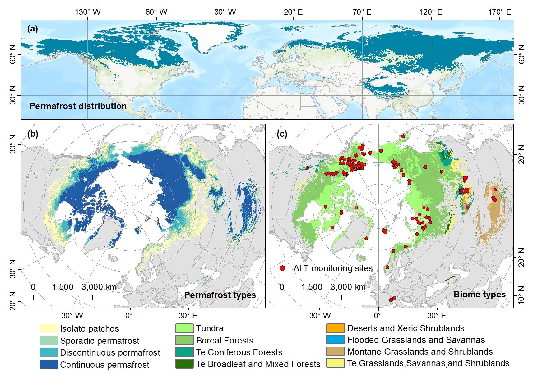
Figure 1 Distribution range of permafrost regions in the Northern Hemisphere (a), distribution of permafrost types (b), biome types and ALT sites (c). Te = Temperate.

The permafrost distribution used in this study was obtained from the 1 km Northern Hemisphere permafrost dataset developed by Obu et al. (2019), which represents near-surface permafrost conditions for 2000–2016. The continuous, discontinuous, sporadic, and isolated-patch permafrost classes were combined to define the spatial domain of the reconstruction. This permafrost extent was applied as a fixed mask to all annual ALT maps from 2000 to 2024; therefore, the dataset represents temporal changes in ALT within the mapped permafrost domain rather than changes in permafrost extent itself. The dataset is publicly accessible via PANGAEA (Obu et al., 2018).

2.2 ALT observations

ALT observations were compiled from the Circumpolar Active Layer Monitoring (CALM) program and the Global Terrestrial Network for Permafrost (GTN-P) to support model development and evaluation across the Northern Hemisphere permafrost region. Measurements were obtained using established monitoring approaches, including mechanical probing near the end of the thawing season, borehole ground-temperature profiles where thaw depth exceeded the practical probing range, and thaw tubes (Peng et al., 2023). In this study, ALT follows the operational definition used by CALM/GTN-P and refers to the annual maximum thaw depth reached in a given year. Where the ground fully refreezes during winter, this quantity corresponds to classical active layer thickness, whereas under persistent talik conditions it may approach the depth to the permafrost table.

The monitoring network spans broad geographic and environmental gradients but remains spatially uneven (Fig. 1), with relatively dense clusters in Alaska and parts of the Eurasian Arctic, whereas observations are sparser or discontinuously distributed across northern Canada, Greenland, interior Siberia, and the Tibetan Plateau. A multi-step quality-control procedure was applied before model development. Records with missing or implausible coordinates, duplicated entries, incomplete site information, or unresolved inconsistencies in site location, observation year, or ALT value were removed. Exceptionally deep thaw-depth records were subjected to additional screening. Isolated extreme values, abrupt discontinuities relative to adjacent years, and extreme records from very short site series without sufficient temporal support were excluded. In contrast, persistently high and temporally consistent records were retained to avoid artificially truncating the upper tail of the observed ALT distribution.

2.3 Environmental variables

To reconstruct annual ALT across the Northern Hemisphere, we compiled a multi-source environmental predictor dataset consisting of 17 environmental variables, including nine time-varying drivers and eight time-invariant environmental controls. These predictors were selected to represent climatic, vegetation, topographic, soil, and ecosystem conditions associated with ALT variability. All raster datasets were reprojected to a common coordinate reference system, clipped to the Northern Hemisphere permafrost extent, and resampled to a common 1 km grid before model development. Detailed information on data sources, and native spatial and temporal resolutions is provided in Table S1 in the Supplement.

Prior to model development, the continuous candidate predictors were screened using Pearson correlation analysis to reduce feature redundancy and potential multicollinearity. Predictors showing strong collinearity with retained variables or only weak associations with ALT were excluded. This screening resulted in a final set of 12 predictors: SR, MAT, MAP, SDE, TI, NDVI, Biome, Elev, Slope, BD, CF, and Silt. Detailed correlation results are provided in Fig. S1 in the Supplement.

2.3.1 Time-varying drivers

Dynamic predictors were used to characterize the interannual variability of climate and vegetation associated with ALT dynamics. Climate-related variables included mean annual temperature (MAT), annual maximum monthly mean temperature (MATmax), annual minimum monthly mean temperature (MATmin), mean annual precipitation (MAP), thawing index (TI), freezing index (FI), solar radiation (SR), and snow depth (SDE).

Monthly average maximum temperature (t_max), monthly average minimum temperature (t_min), and total monthly precipitation for 2000–2024 were obtained from the WorldClim historical monthly weather dataset, which provides downscaled monthly climate data based on WorldClim v2.1. Monthly mean air temperature was calculated as the average of monthly t_max and t_min. MAT was subsequently calculated as the average of the 12 monthly mean temperatures, whereas MAP was calculated as the sum of monthly precipitation. MATmax and MATmin were defined as the maximum and minimum monthly mean temperatures within each year, respectively. The TI and FI were derived from monthly mean air temperature by weighting each monthly value by the number of days in the corresponding month. Specifically,

$$\begin{array}{}\text{(1)}& {\displaystyle }& {\displaystyle }\mathrm{TI}=\sum _{i=\mathrm{1}}^{\mathrm{12}}\max \left(T_i,\mathrm{0}\right)\times D_i\text{(2)}& {\displaystyle }& {\displaystyle }\mathrm{FI}=\sum _{i=\mathrm{1}}^{\mathrm{12}}\left|\min \left(T_i,\mathrm{0}\right)\right|\times D_i\end{array}$$

where T_i is the monthly mean air temperature of month i, and D_i is the corresponding number of days in that month. TI and FI represent the annual cumulative positive and negative degree-days, respectively.

Monthly SR and SDE were obtained from the ERA5-Land reanalysis dataset. Annual SR was calculated as the mean of the 12 monthly values, whereas winter SDE was calculated as the average snow depth from October of the previous year through April of the current year, representing snow conditions during the cold season that predominantly influence subsequent active layer development. Accordingly, winter SDE for 2000 was calculated using ERA5-Land snow-depth data from October–December 1999 and January–April 2000. Vegetation dynamics were represented by the annual maximum normalized difference vegetation index (NDVI), obtained from the Global 1 km Resolution Annual Maximum Composite NDVI Dataset (V3) (Wang et al., 2026). For each ALT observation, the corresponding annual values of all dynamic predictors were extracted according to the observation year to ensure temporal consistency between predictor variables and ALT measurements.

2.3.2 Time-invariant environmental controls

Time-invariant predictors were used to characterize the spatial heterogeneity of terrain, soil, and ecosystem conditions. Topographic variables included elevation (Elev) and slope (Slope). Elevation was obtained from the General Bathymetric Chart of the Oceans (GEBCO) global elevation dataset, and slope was subsequently derived from the elevation using standard terrain analysis procedures. Biome type (Biome) was additionally included as a categorical predictor to represent broad differences in vegetation communities and ecosystem conditions across the Northern Hemisphere permafrost region (Olson et al., 2001).

Soil properties were obtained from the SoilGrids database and included bulk density (BD), coarse fragment content (CF), sand content (Sand), silt content (Silt), and clay content (Clay). SoilGrids provides these properties for six standard depth intervals (0–5, 5–15, 15–30, 30–60, 60–100, and 100–200 cm). For each soil variable, a thickness-weighted mean over 0–200 cm was calculated and used as the static soil predictor. The 0–200 cm interval was selected because it represents the deepest consistently available SoilGrids profile and provides an integrated characterization of near-surface substrate conditions relevant to active-layer thermal and hydrological processes. Although ALT exceeds 2 m at some monitoring locations, these soil variables were used as background descriptors rather than as a depth-resolved representation of the full seasonally thawed layer. A sensitivity analysis was additionally conducted using thickness-weighted soil properties integrated over 0–30, 0–100, and 0–200 cm. Spatial block cross-validation showed only minor performance differences among the three configurations, with nearly identical results for the 0–100 and 0–200 cm profiles (Table S2).

2.4 Spatiotemporal reconstruction of ALT

2.4.1 Construction of the modelling dataset

A spatiotemporal feature-matching strategy was used to construct the modelling dataset. For each ALT observation, annual dynamic environmental covariates were extracted for the corresponding observation year, while static topographic and soil properties were assigned according to the station location. Some records were located near water bodies, outside the valid coverage of individual remote-sensing products, or in areas with missing soil or vegetation information. Records containing missing values in any retained predictor were therefore excluded to ensure a complete and internally consistent modelling dataset. After data matching, quality control, and predictor screening, 2373 annual ALT records from 199 monitoring sites during 2000–2024 were retained. Observations from 2000–2020 were used for spatial model development and cross-validation, whereas newly compiled observations from 2021–2024 were initially withheld for temporally blocked validation. After this evaluation, the full 2000–2024 observational dataset was used to train the final model.

2.4.2 Model development and spatial validation

Five machine-learning algorithms were evaluated as candidate models: Random Forest (RF), Gradient Boosting Decision Tree (GBDT), eXtreme Gradient Boosting (XGBoost), Categorical Boosting (CatBoost), and Light Gradient Boosting Machine (LightGBM). Biome was treated as a categorical predictor and transformed using one-hot encoding before model training to avoid imposing an artificial ordinal relationship among biome classes. Model configurations were established during preliminary model development and fixed before validation, and the parameter settings adopted for the machine learning algorithms are provided in Table S3.

Spatial block cross-validation was first conducted using observations from 2000–2020 to assess model transferability across geographically separated regions. Monitoring sites were assigned to 10°×10° latitude–longitude blocks, and in each fold all observations from sites within one block were withheld while observations from the remaining blocks were used for model training. The 10°×10° block size represented a compromise between increasing spatial separation and retaining sufficient populated blocks and validation observations given the uneven distribution of monitoring sites. Model performance was evaluated using the coefficient of determination (R²), root mean square error (RMSE), mean absolute error (MAE), Lin's concordance correlation coefficient (CCC) (Lin, 1989), and mean bias. Bias was defined as predicted minus observed ALT, with positive and negative values indicating overestimation and underestimation, respectively. CCC was calculated as:

$$\begin{array}{}\text{(3)}& \mathrm{CCC}={\displaystyle \frac{\mathrm{2}r{\partial }_y{\partial }_{\widehat{y}}}{{\partial }_y^{\mathrm{2}}+{\partial }_{\widehat{y}}^{\mathrm{2}}+{\left(\stackrel{\mathrm{‾}}{y}-\stackrel{\mathrm{‾}}{\widehat{y}}\right)}^{\mathrm{2}}}}\end{array}$$

where r is the Pearson correlation coefficient between observed and predicted values, ∂_y and ${\partial }_{\widehat{y}}$ are their standard deviations, and $\stackrel{\mathrm{‾}}{y}$ and $\stackrel{\mathrm{‾}}{\widehat{y}}$ are their means.

Based on their overall spatial block cross-validation performance and complementary predictive behaviour, XGBoost and LightGBM were selected for ensemble construction, and the ensemble prediction was calculated as the arithmetic mean of the selected model predictions.

After the ensemble configuration was fixed, leave-one-site-out cross-validation (LOSO-CV) was conducted as a complementary site-level assessment. In each fold, all annual observations from one monitoring site were withheld simultaneously, and the ensemble model was trained using observations from all remaining sites. Overall LOSO-CV performance was evaluated by pooling the out-of-fold predictions and calculating R², RMSE, MAE, CCC, and bias. Because sites with longer records contribute more observations to the pooled statistics, site-level RMSE, MAE, and bias were also calculated separately for each monitoring site and summarized using their mean and median values.

2.4.3 Temporal extrapolation validation

To evaluate model transfer beyond the historical calibration period, an additional temporally blocked validation was conducted. All observations from 2000–2020 were used for model training, whereas the newly compiled observations from 2021–2024 were completely withheld from model fitting and used as an independent post-calibration test set.

The models trained exclusively on the 2000–2020 observations were applied to the corresponding environmental predictors for 2021–2024, and predictions were evaluated against the withheld ALT observations using R², RMSE, MAE, CCC, and bias. Performance was assessed for two subsets: (1) all available 2021–2024 observations, including both previously observed and newly observed sites, and (2) observations restricted to sites already represented during 2000–2020. The first evaluation therefore reflects temporal transfer together with spatial generalization for newly observed sites, whereas the second provides a more direct assessment of temporal transfer at previously monitored locations.

2.4.4 Temporal performance at long-term monitoring sites

To evaluate the temporal performance of the reconstructed ALT dataset at spatially withheld locations, site-level out-of-fold predictions generated by LOSO-CV were used. This analysis focused on long-term monitoring sites because short and highly fragmented records may not provide stable estimates of temporal change. Only sites with at least 10 valid annual ALT observations and an observation span exceeding 15 years during 2000–2020 were retained, resulting in 60 long-term monitoring sites.

For each year, annual monitoring-network mean observed and predicted ALT values were calculated using the paired site-year records available across the selected long-term sites. The temporal correspondence between the two regional mean time series was evaluated using the Pearson correlation coefficient (r), coefficient of determination (R²), and root mean square error (RMSE). Long-term change was further characterized using Sen's slope calculated separately for the observed and predicted regional mean ALT time series. This comparison was used to assess whether the model reproduced the overall direction and magnitude of long-term ALT change across the monitoring network.

Site-level temporal trends were additionally evaluated to characterize spatial variability in long-term model performance. Sen's slopes were calculated separately for the observed and LOSO-predicted ALT time series at each monitoring site. Trend performance was summarized using the proportion of sites with consistent observed and predicted trend directions and the mean absolute Sen's slope error (MASE):

$$\begin{array}{}\text{(4)}& \mathrm{MASE}={\displaystyle \frac{\mathrm{1}}{n}}\sum _{i=\mathrm{1}}^n\left|{\mathit{\beta }}_{\mathrm{pred},i}-{\mathit{\beta }}_{\mathrm{obs},i}\right|\end{array}$$

where β_pred,i and β_obs,i denote the Sen's trend slopes of the predicted and observed ALT time series at the ith monitoring site, respectively, and n is the number of validation sites.

The ability of the model to reproduce interannual ALT variability was evaluated using the fluctuation amplitude ratio (FAR). For each site, linear trends were first removed from the observed and predicted ALT time series, and FAR was calculated as:

$$\begin{array}{}\text{(5)}& \mathrm{FAR}={\displaystyle \frac{{\mathit{\sigma }}_{\mathrm{pred},\mathrm{detrended}}}{{\mathit{\sigma }}_{\mathrm{obs},\mathrm{detrended}}}}\end{array}$$

where σ_{pred,detrended} and σ_{obs,detrended} are the standard deviations of the detrended predicted and observed ALT time series, respectively. FAR values close to 1 indicate comparable fluctuation amplitudes, whereas values below or above 1 indicate underestimation or overestimation of interannual variability. Overall performance was summarized using the median FAR across all long-term sites.

In addition to these quantitative evaluations, time-series comparisons were presented for selected representative long-term monitoring sites to illustrate site-level differences between observations, LOSO-CV predictions, and predictions from the final model trained using the complete observational dataset.

2.4.5 Dataset production

After the predictor set, model configuration, ensemble rule, and validation framework had been finalized, XGBoost and LightGBM were refitted using the complete quality-controlled observational dataset spanning 2000–2024. The two full-data models were then applied to the corresponding annual environmental covariates to generate annual ALT maps for the Northern Hemisphere permafrost region from 2000 to 2024. The final ALT estimate for each grid cell and year was calculated as the arithmetic mean of the XGBoost and LightGBM predictions.

2.5 Site-resampling uncertainty quantification

Uncertainty associated with the spatial composition of the monitoring network was quantified using repeated site-level subsampling. After the predictor set, model configurations, and ensemble rule had been fixed, 80 % of the monitoring sites were randomly selected without replacement in each realization, with all annual observations from the selected sites retained together. This procedure was repeated 100 times to generate 100 site-resampled training datasets.

For each realization, XGBoost and LightGBM were refitted separately using the corresponding subsampled dataset and applied to the annual environmental covariates. Predictions from the two models were averaged to obtain one ensemble ALT realization for each grid cell and year. For each grid cell, the 2.5th and 97.5th percentiles of the 100 ensemble predictions were taken as the lower and upper bounds of an empirical 95 % site-resampling interval. This interval characterizes the sensitivity of model predictions to changes in the composition of the monitoring-site network and should not be interpreted as a complete predictive uncertainty interval (Wei et al., 2025).

Relative site-resampling uncertainty was calculated by normalizing the width of the empirical prediction interval by the mean ensemble prediction:

$$\begin{array}{}\text{(6)}& \mathrm{RU}={\displaystyle \frac{Q_{\mathrm{97.5}}-Q_{\mathrm{2.5}}}{{\mathrm{ALT}}_{\mathrm{mean}}}}\times \mathrm{100}\mathit{\%}\end{array}$$

where RU is the relative site-resampling uncertainty; Q_97.5 and Q_2.5 are the 97.5th and 2.5th percentiles of the 100 site-resampled ensemble predictions, respectively, and ALT_mean is their mean. Lower RU values indicate lower sensitivity to changes in training-site composition, whereas higher values indicate greater variation among the site-resampled model realizations. This metric does not explicitly account for other sources of predictive uncertainty, including measurement error in ALT observations, uncertainty in environmental predictors, residual model error, unresolved sub-grid heterogeneity, or temporal extrapolation.

2.6 Area of applicability

The area of applicability (AOA) was assessed following the general framework of Meyer and Pebesma (2021), with two adaptations: predictor weights were derived from SHAP importance of the final ensemble model, and the AOA threshold was defined using spatial block cross-validation. Continuous predictors were standardized using the mean and standard deviation of the calibration samples. Biome was represented by the same one-hot-encoded binary indicators used for model training. Environmental dissimilarity was quantified using a SHAP-weighted Euclidean distance in the encoded predictor space. SHAP importance was first calculated separately for each model input feature, including individual biome dummy variables, and the resulting relative mean absolute SHAP values were used as feature weights in the distance calculation. For presentation of overall predictor importance, SHAP contributions of the biome dummy variables were subsequently summed to obtain a single Biome contribution. For each prediction pixel, the minimum weighted distance to the calibration samples was taken as the dissimilarity index (DI).

The DI threshold was determined from the 10°×10° spatial block cross-validation. For each fold, DI values for samples in the withheld block were calculated relative only to samples in the corresponding training blocks. The 95th percentile of the pooled withheld-sample DI distribution was used as the applicability threshold. Pixels with DI values less than or equal to this threshold were classified as inside the AOA, whereas pixels exceeding the threshold were classified as environmental extrapolation.

Because several predictors varied annually, AOA was evaluated separately for each year from 2000 to 2024 using the corresponding annual predictor layers. A temporal AOA frequency was then calculated for each pixel as the proportion of the 25 years classified as inside the AOA. Values approaching 1 indicate environmental conditions that were consistently represented by the calibration data, whereas lower values indicate more frequent environmental extrapolation.

2.7 Statistical analysis of the ALT dataset

Statistical analyses were conducted to characterize the spatial and temporal patterns of the reconstructed ALT dataset. Annual mean ALT across the Northern Hemisphere permafrost domain was calculated for each year from 2000 to 2024. To examine long-term changes in ALT structure, continuous ALT values were classified into predefined depth intervals, and the proportional area of each class was calculated for six selected years. Latitudinal and elevational gradients were analysed by grouping valid permafrost pixels into 5° latitude intervals and elevation bins. To reduce geographic heterogeneity, elevational analyses were performed separately for high-latitude (>60° N, elevation < 2.0 km) and high-elevation regions (25–45° N, elevation > 3.5 km).

The reconstructed ALT dataset was further overlaid with the Northern Hemisphere permafrost zonation map and the global biome dataset. Mean ALT and the distribution of pixel-level ALT values were calculated for each permafrost zone and biome type using all valid overlapping pixels. Differences among categories were visualized using violin plots with embedded boxplots.

3 Results and discussion

3.1 Model performance evaluation

3.1.1 Spatial block cross-validation

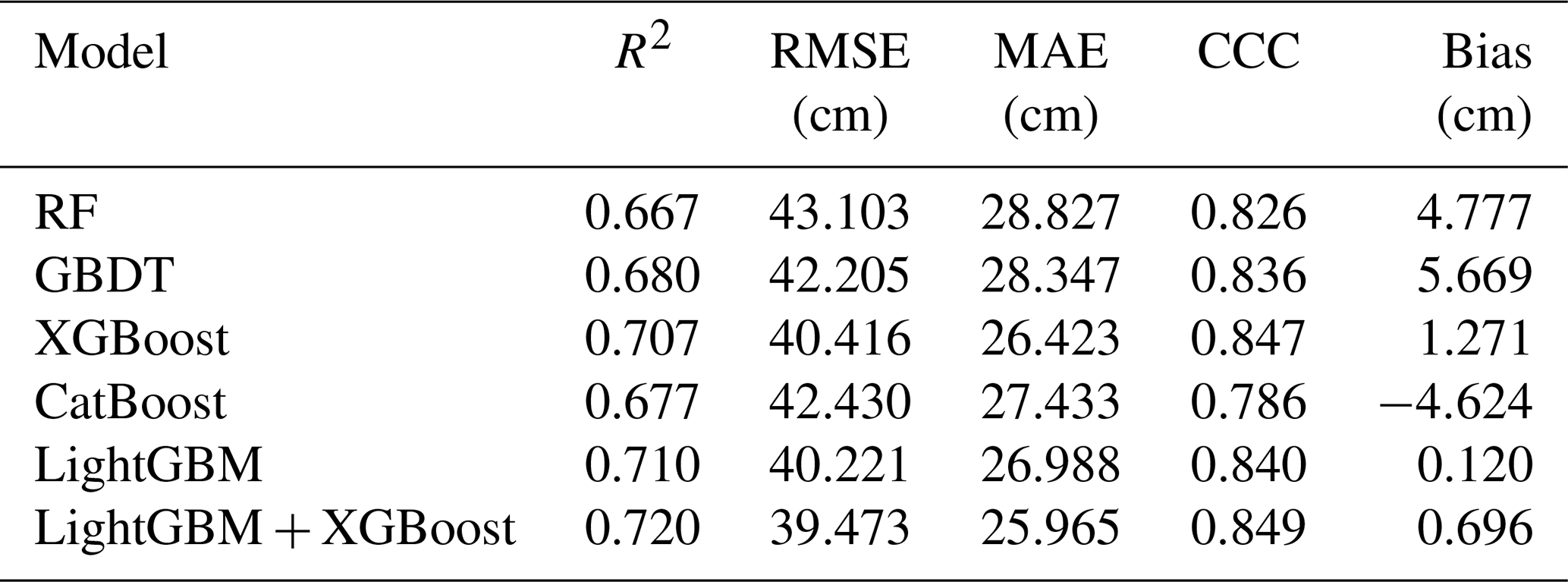
Spatial block cross-validation was used to assess model transferability across geographically separated regions. Spatial block cross-validation showed clear differences among the five candidate models, with R² values of 0.667–0.710, RMSE values of 40.221–43.103 cm, MAE values of 26.423–28.827 cm, and CCC values of 0.786–0.847 (Table 1). LightGBM and XGBoost performed best among the individual models and were therefore combined in the final ensemble. The LightGBM–XGBoost ensemble achieved the highest overall performance, with an R² of 0.720, RMSE of 39.473 cm, MAE of 25.965 cm, CCC of 0.849, and a mean bias of 0.696 cm, and was adopted for subsequent evaluation and dataset production.

Table 1 Performance of the five machine-learning models and the ensemble model under spatial block cross-validation.

Model performance varied substantially across the observed ALT range (Fig. S2; Table S4). For ALT < 100 cm, the ensemble yielded an RMSE of 26.46 cm, an MAE of 17.19 cm, and a bias of 9.43 cm. Errors increased for ALT of 100–300 cm (RMSE = 62.64 cm; MAE = 52.75 cm; bias = −20.56 cm) and were largest for ALT > 300 cm (RMSE = 84.04 cm; MAE = 70.59 cm; bias = −68.12 cm). The increasingly negative bias with increasing ALT indicates a systematic tendency to underestimate deep-thaw conditions.

3.1.2 Leave-one-site-out cross-validation

Leave-one-site-out cross-validation (LOSO-CV) was further used to evaluate the final ensemble model at monitoring locations completely excluded from model training. When all out-of-fold annual predictions were pooled, the LightGBM–XGBoost ensemble achieved an R² of 0.780, an RMSE of 34.981 cm, an MAE of 22.053 cm, a CCC of 0.879, and a mean bias of 1.086 cm (Table S5). The higher performance relative to spatial block cross-validation is consistent with the less stringent spatial separation of LOSO-CV, in which neighbouring or environmentally similar sites may remain in the training dataset.

To reduce the influence of unequal record lengths among monitoring sites, errors were also summarized at the site level (Table S5). The median site-level RMSE and MAE were 17.173 and 15.827 cm, respectively, compared with mean values of 31.295 and 29.847 cm. The higher mean than median errors indicate that prediction errors were relatively small at many sites but substantially larger at a subset of locations (Fig. S3). Site-level bias remained close to zero overall, with a median of 1.325 cm and a mean of −1.080 cm.

3.1.3 Temporal blocked validation

Temporal blocked validation was conducted to assess model transferability beyond the historical training period. The ensemble model was trained exclusively using observations from 2000–2020, while all available observations from 2021–2024 were withheld for evaluation. Across all withheld records, including both previously observed and newly observed sites, the model achieved an R² of 0.693, an RMSE of 26.36 cm, an MAE of 17.55 cm, a CCC of 0.802, and a mean bias of 0.51 cm (Fig. S4a).

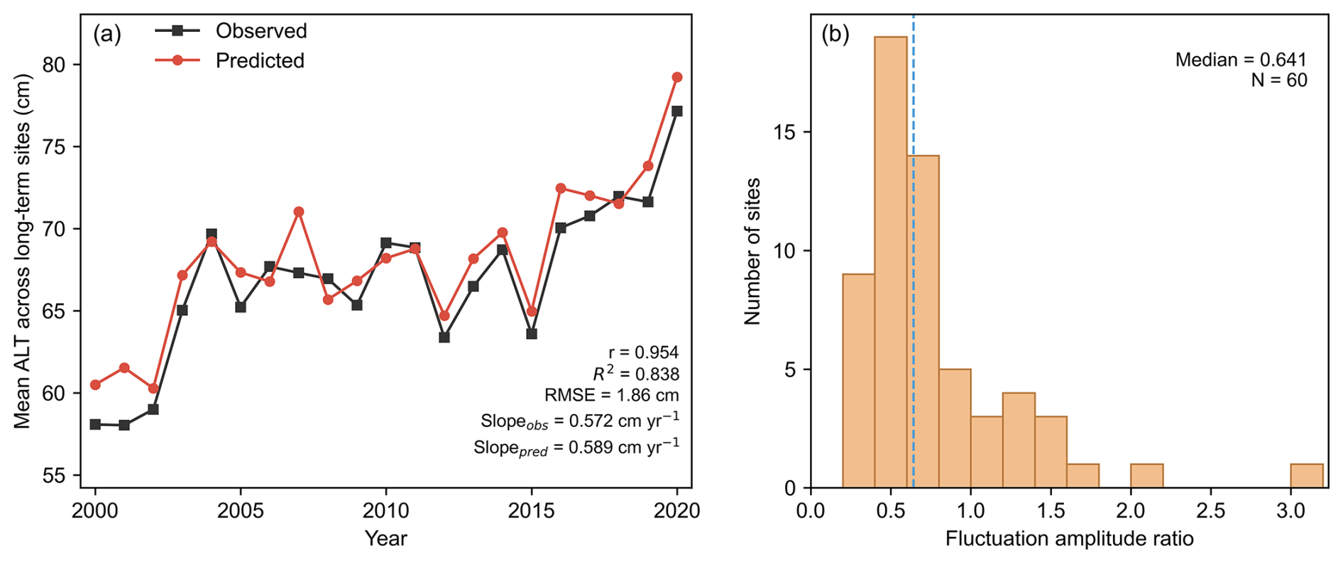
Figure 2 Temporal performance of LOSO-CV predictions at 60 long-term monitoring sites during 2000–2020. (a) Annual mean observed and predicted ALT calculated from paired site-year records across the long-term monitoring network. (b) Distribution of the fluctuation amplitude ratio (FAR) calculated from detrended observed and predicted ALT series at individual monitoring sites. The dashed vertical line indicates the median FAR (0.641).

When the evaluation was restricted to sites already represented during 2000–2020, performance was higher, with an R² of 0.826, an RMSE of 19.74 cm, an MAE of 14.06 cm, a CCC of 0.895, and a mean bias of 0.13 cm (Fig. S4b). The lower performance for the complete 2021–2024 test set reflects the additional challenge of predicting newly observed sites, which requires both temporal transfer to subsequent years and spatial generalization to previously unseen locations. These results indicate that relationships learned from the 2000–2020 observations remained transferable to subsequent years, while prediction errors increased when temporal and spatial extrapolation occurred simultaneously.

3.1.4 Long-term temporal dynamics

The LOSO-derived predictions reproduced the common temporal evolution across the 60 long-term monitoring sites (Fig. 2a). The annual mean ALT calculated from paired observations and predictions showed close temporal correspondence, with a Pearson correlation coefficient of 0.954, an R² of 0.838, and an RMSE of 1.861 cm. The Sen's slopes of the observed and predicted mean series were also similar, at 0.572 and 0.589 cm yr⁻¹, respectively, indicating that the model reproduced the overall long-term increase in ALT across the monitoring network.

At the individual-site level, 86.7 % of the monitoring sites showed consistent trend directions between observations and LOSO-CV predictions, with a mean absolute Sen's slope error of 0.343 cm yr⁻¹. However, interannual variability was generally underestimated. The median fluctuation amplitude ratio (FAR) across the 60 sites was 0.641 (Fig. 2b), with most sites exhibiting FAR values below 1, indicating substantial smoothing of year-to-year ALT fluctuations at individual locations. Time-series comparisons at six representative long-term monitoring sites further illustrated the range of site-specific temporal behaviour (Fig. S5). Overall, the model reproduced the common long-term temporal signal more effectively than site-specific year-to-year variability.

3.2 Spatiotemporal pattern of ALT

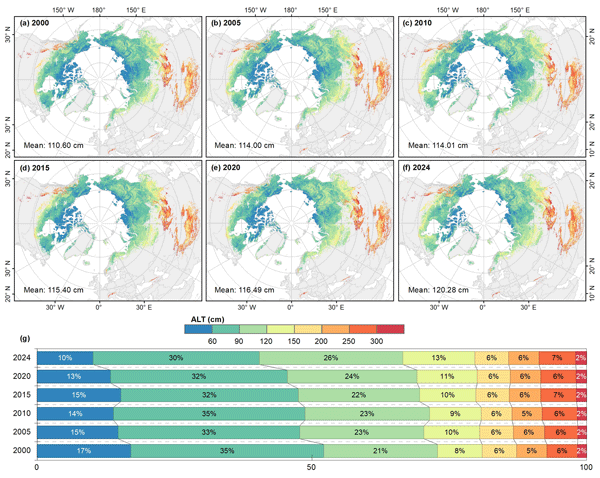
Based on the final ensemble model, annual ALT was reconstructed across the Northern Hemisphere permafrost region from 2000 to 2024 (Fig. 3). ALT showed pronounced spatial heterogeneity, with generally shallower values at high latitudes and deeper values toward lower-latitude and marginal permafrost regions. Values were typically below 100 cm across northern Siberia, the Canadian Arctic Archipelago, and northern Alaska, but exceeded 250 cm in several warmer or high-elevation marginal regions, including parts of the Mongolian Plateau, Transbaikal, and the Tibetan Plateau.

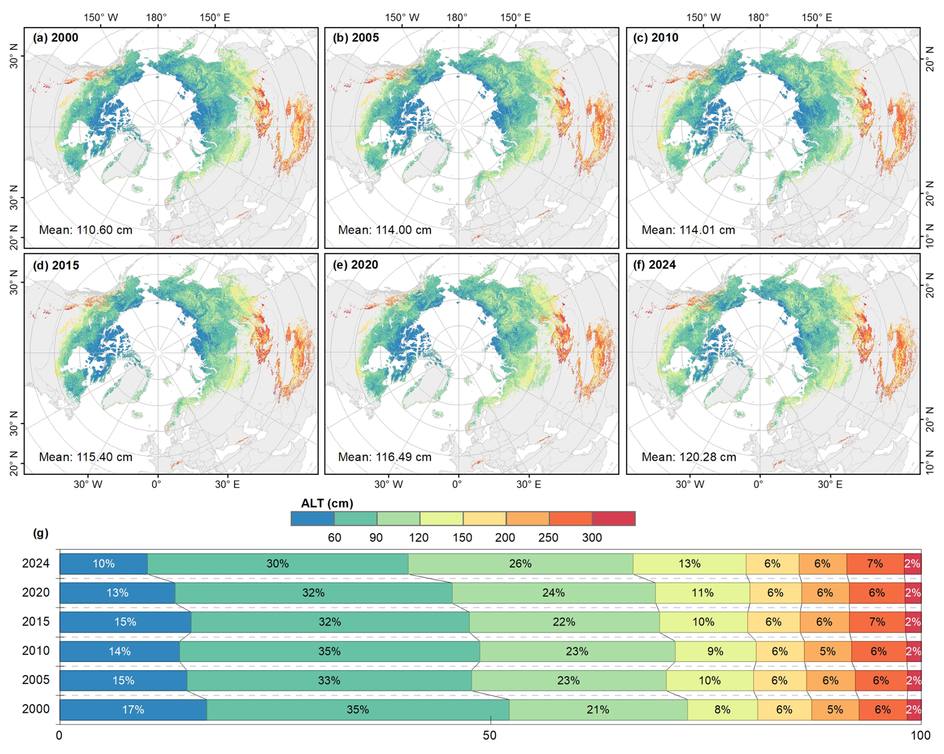
Figure 3 Spatiotemporal distribution of ALT (a–f) and the proportion of ALT area at different levels (g) from 2000 to 2024.

The spatial mean ALT increased from 110.60 cm in 2000 to 120.28 cm in 2024, corresponding to a net increase of 9.68 cm (Fig. 3a–f). Mean ALT increased to 114.00 cm by 2005, changed relatively little during 2005–2020, and then rose to 120.28 cm by 2024, indicating an overall long-term deepening of seasonal thaw.

The ALT-class distribution also shifted away from shallow conditions (Fig. 3g). Areas with ALT < 60 cm and 60–90 cm decreased from 17 % and 35 % in 2000 to 10 % and 30 % in 2024, whereas the 90–120 and 120–150 cm classes increased from 21 % to 26 % and from 8 % to 13 %, respectively. Changes in classes above 150 cm were comparatively small. Overall, the redistribution was characterized mainly by a contraction of shallow ALT areas and an expansion of intermediate ALT conditions.

3.3 Geographic and ecological patterns of ALT

ALT exhibited pronounced geographic gradients across the reconstructed domain (Fig. 4). Median ALT generally exceeded 200 cm between 25 and 50° N and reached approximately 250–260 cm at 40–45° N, whereas north of 50° N it declined markedly with latitude to about 55–80 cm at 70–85° N (Fig. 4a). This nonlinear pattern reflects the contrast between lower-latitude high-mountain permafrost and high-latitude Arctic environments.

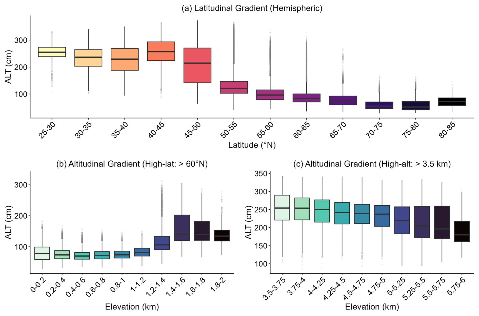
Figure 4 Macro-scale topographic and latitudinal patterns of ALT (Average value from 2000 to 2024). (a) Hemispheric ALT distribution along the latitudinal gradient (binned at 5° intervals). (b) ALT variation along the altitudinal gradient in high-latitude Arctic regions (north of 60° N). (c) ALT variation along the altitudinal gradient in high-altitude, mid-to-low latitude regions (elevation > 3.5 km, typified by the Tibetan Plateau).

Altitudinal relationships differed between these settings. North of 60^∘N, median ALT remained around 70–80 cm below 1.0 km elevation but increased to approximately 135–145 cm above 1.4 km (Fig. 4b), potentially reflecting differences in drainage, organic-layer development, and substrate conditions between low- and high-elevation Arctic landscapes (Rouse, 2000; Pan et al., 2016; Si et al., 2024). In contrast, ALT decreased with elevation in high-altitude regions above 3.5 km, from approximately 250–255 cm at 3.5–4.0 km to about 180 cm at 5.75–6.0 km (Fig. 4c), consistent with colder conditions and reduced seasonal thaw at higher elevations (Karki et al., 2020). These contrasting gradients support the physical plausibility of the reconstructed large-scale ALT patterns.

ALT also varied systematically across permafrost zones and biome types (Fig. 5). Mean ALT increased from 100.52 cm in continuous permafrost to 123.29, 128.25, and 130.51 cm in discontinuous, sporadic, and isolated-patch permafrost, respectively (Fig. 5a). The relatively small differences and substantial overlap among the latter three classes indicate considerable within-zone variability despite the overall increase toward less continuous permafrost.

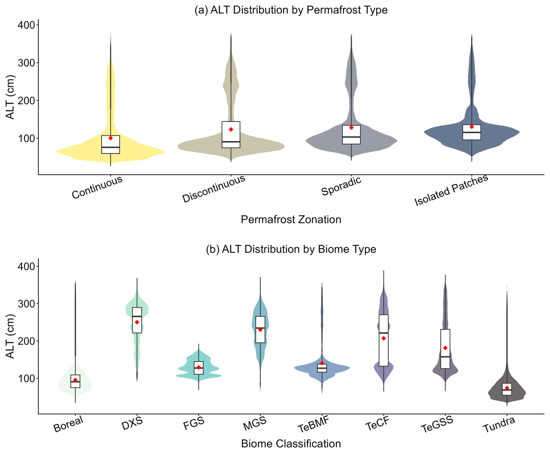
Figure 5 Statistical distribution of ALT across different permafrost zones and biome types. In each panel, the shaded violin shape represents the full probability density distribution of pixel-wise ALT predictions. Within the nested boxplots, the horizontal solid line indicates the median, the box boundaries represent the interquartile range (25th to 75th percentiles), and the red diamonds denote the arithmetic means. DXS = Deserts and Xeric Shrublands; FGS = Flooded Grasslands and Savannas; MGS = Montane Grasslands and Shrublands; TeBMF = Temperate Broadleaf and Mixed Forests; TeCF = Temperate Coniferous Forests; TeGSS = Temperate Grasslands, Savannas, and Shrublands.

Among biome types, tundra and boreal forest had the shallowest mean ALT values (74.19 and 95.64 cm), whereas deserts and xeric shrublands (DXS) and montane grasslands and shrublands (MGS) had the deepest values (250.21 and 230.06 cm, respectively) (Fig. 5b). Intermediate values occurred in FGS (129.18 cm), TeBMF (140.71 cm), TeGSS (181.40 cm), and TeCF (206.95 cm). These contrasts are consistent with broad differences in thermal regime, moisture availability, vegetation cover, and soil conditions among biome types.

3.4 Site-resampling uncertainty and area of applicability

The site-resampling uncertainty showed a generally stable magnitude and spatial pattern during 2000–2024 (Figs. 6a and S6). Mean relative uncertainty was 45.29 % over the study period, with values for the selected years varying only slightly from 45.08 % to 45.76 %. The proportional distribution among uncertainty classes was similarly stable: approximately 64 %–65 % of the mapped permafrost area had relative uncertainty between 20 % and 50 %, whereas only about 8 %–9 % exceeded 70 % (Fig. S6). Spatially, lower site-resampling uncertainty occurred across extensive parts of Alaska, northern Canada, Siberia, and the Tibetan Plateau, while higher values were distributed more discontinuously across several regions. These spatial differences indicate varying sensitivity of the predictions to the composition of the monitoring network rather than differences in total predictive reliability.

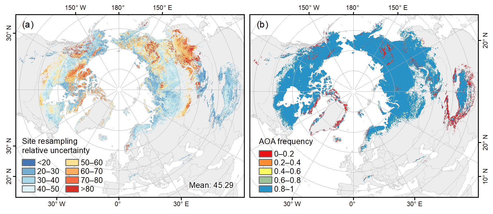
Figure 6 Spatial distributions of mean site-resampling uncertainty and area-of-applicability frequency during 2000–2024. (a) Mean relative site-resampling uncertainty across 2000–2024 (units: %). (b) Frequency of years during 2000–2024 in which each pixel was classified as within the area of applicability (AOA).

The area-of-applicability (AOA) analysis provided complementary information on environmental extrapolation (Fig. 6b). Most of the mapped permafrost domain had AOA frequencies of 0.8–1.0, indicating that environmental conditions remained within the calibration domain during most years from 2000 to 2024. Lower AOA frequencies occurred in more localized areas, indicating regions where predictions more frequently involved extrapolation beyond the environmental space represented by the observations. Importantly, low site-resampling uncertainty does not necessarily imply high predictive reliability in data-sparse regions, because different resampled models may produce similar predictions even outside well-represented environmental conditions. The uncertainty and AOA layers should therefore be interpreted jointly when assessing the spatial applicability of the dataset.

This distinction is particularly relevant for permafrost regions where local thaw conditions are influenced by heterogeneous soil, snow, vegetation, ground-ice, and hydrological properties that cannot be fully resolved by kilometre-scale predictors. These diagnostics are particularly relevant for applications linking permafrost thaw to carbon-cycle and ecosystem processes, for which spatially heterogeneous thaw conditions can propagate into downstream analyses (Hugelius et al., 2014; Schuur et al., 2015). Accordingly, the site-resampling uncertainty and AOA information provide complementary guidance for regional- to hemispheric-scale applications of the ALT dataset, including carbon-cycle and ecosystem studies.

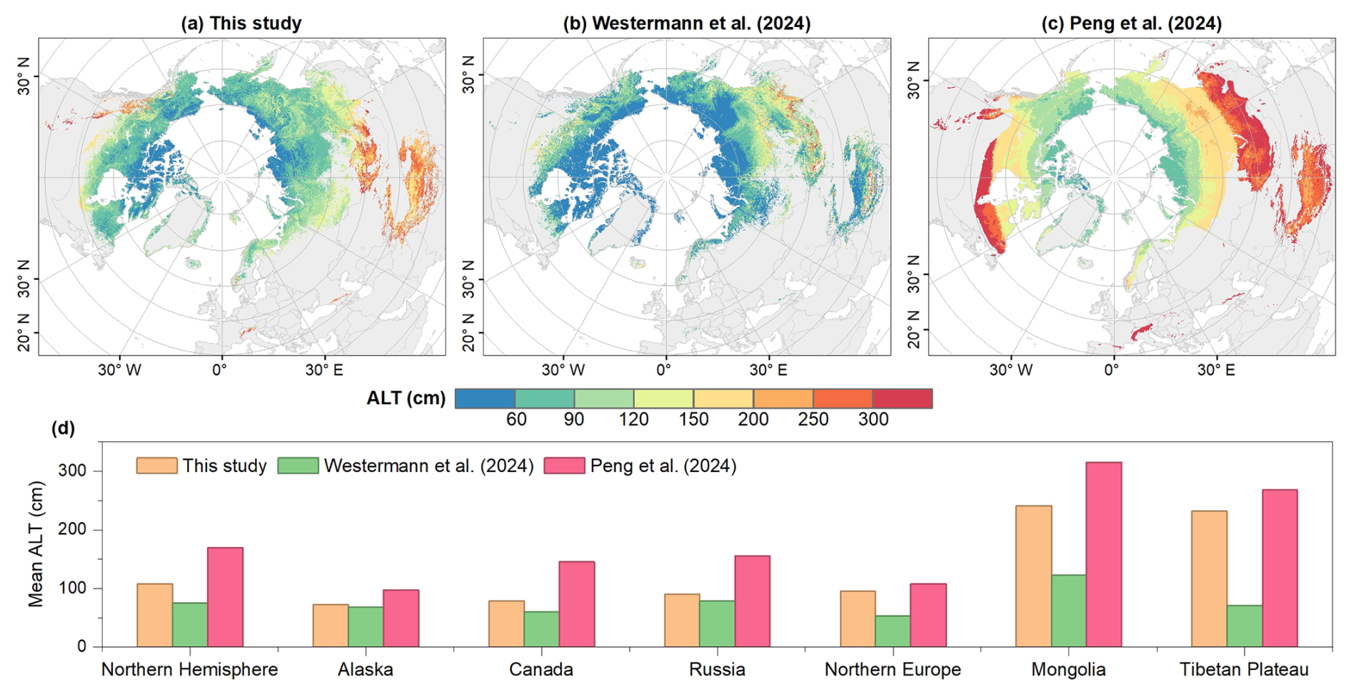
Figure 7 Spatial patterns and harmonized hemispheric and regional mean active layer thickness (ALT) during 2000–2020 for this study and two existing hemispheric products. (a–c) Mean ALT distributions from this study, Westermann et al. (2024), and Peng et al. (2024), respectively, shown over the valid spatial domain of each product. (d) Mean ALT for the Northern Hemisphere and selected regions calculated using pixels valid in all three products. All statistics in panel (d) were derived over the common period 2000–2020 and an identical three-product common-valid spatial domain.

3.5 Comparison with other datasets

To contextualize the reconstructed dataset, we compared it with two recently published 1 km hemispheric ALT products: the physics-based product of Westermann et al. (2024) and the machine-learning product of Peng et al. (2024) (Figs. 7 and 8). All comparisons were restricted to the common period 2000–2020. The spatial maps in Fig. 7a–c retain the valid domain of each individual product to illustrate their overall spatial patterns, whereas the hemispheric and regional statistics in Fig. 7d were calculated using pixels valid in all three products to ensure an identical spatial comparison domain.

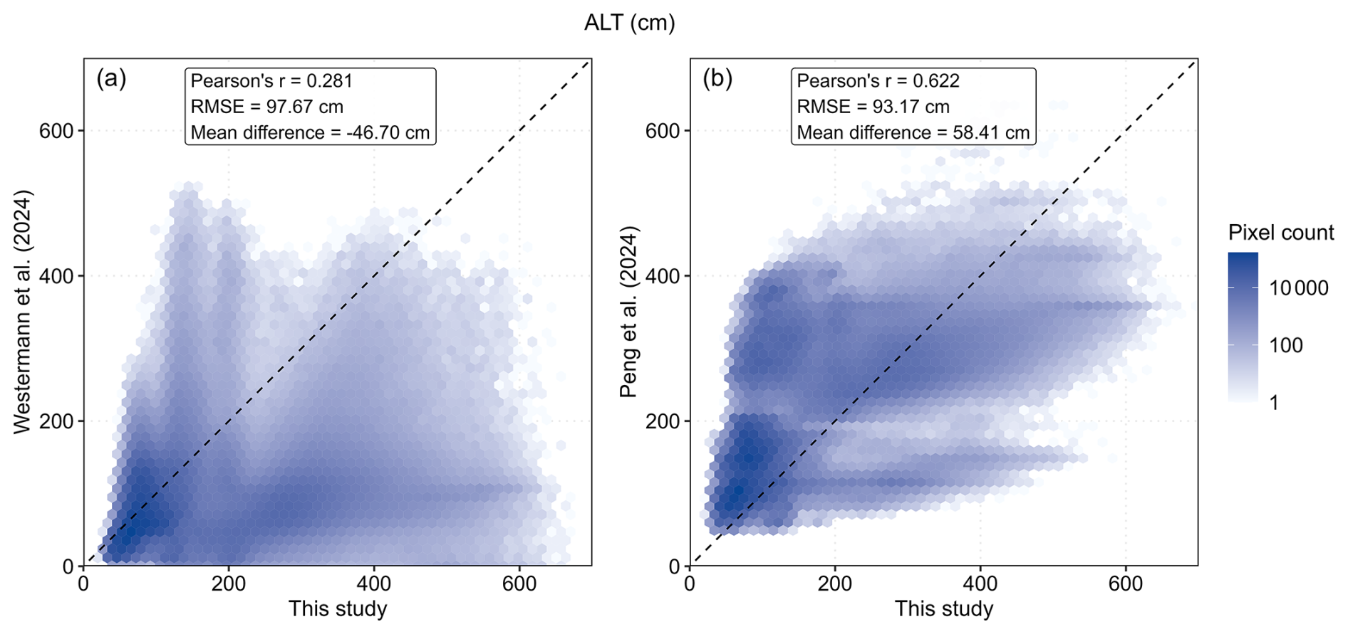
Figure 8 Pixel-wise comparison of mean ALT during 2000–2020 between this study and two existing hemispheric products. (a) Westermann et al. (2024) and (b) Peng et al. (2024), each compared with this study using 5 million randomly sampled common valid pixels. Dashed lines indicate the 1:1 relationship. RMSE and mean difference represent inter-product disagreement, with mean difference calculated as the existing product minus this study.

The three products exhibited substantial differences in ALT magnitude and spatial structure (Fig. 7). Over the harmonized three-product domain, mean ALT was 107.87 cm in this study, compared with 74.96 cm for Westermann et al. (2024) and 169.72 cm for Peng et al. (2024). The same general ordering occurred across most regions, although the magnitude of inter-product differences varied substantially (Table S6). Differences were relatively small in Alaska, where mean ALT ranged from 68.05 to 97.82 cm, but were much larger in Mongolia and the Tibetan Plateau. For example, mean ALT over the Tibetan Plateau was 232.09 cm in this study, compared with 71.27 cm in Westermann et al. (2024) and 268.08 cm in Peng et al. (2024).

Pairwise pixel-level comparisons further revealed substantial inter-product disagreement (Fig. 8). Spatial agreement was stronger with Peng et al. (2024) (r=0.622) than with Westermann et al. (2024) (r=0.281), although RMSE remained high in both comparisons (93.17 and 97.67 cm, respectively). Mean differences, calculated as the existing product minus this study, were −46.70 cm for Westermann et al. (2024) and 58.41 cm for Peng et al. (2024), consistent with their generally shallower and deeper estimates, respectively. These comparisons represent inter-product agreement rather than independent validation, and the remaining discrepancies likely reflect differences in model formulation, predictor information, spatial domains, and the representation of deep thaw and talik conditions.

3.6 Potential applications and limitations

This study provides an annual ALT dataset on a 1 km grid for the Northern Hemisphere permafrost region from 2000 to 2024. The dataset is intended primarily for regional- to hemispheric-scale analyses of spatial ALT patterns and long-term changes. When combined with complementary soil, ecosystem, climate, and socioeconomic datasets, it can support investigations of permafrost carbon feedbacks, vegetation and hydrological responses to thaw, and broad-scale assessments of infrastructure exposure (Schuur et al., 2015; Harris et al., 2023; Lathrop et al., 2025; Mishra et al., 2021; Mu et al., 2016). It can also provide baseline information for identifying areas where increasing thaw depth may elevate risks to roads, railways, pipelines, and settlements (Gartler et al., 2025; Jin et al., 2024; Yang et al., 2010; Hjort et al., 2018).

Several limitations should nevertheless be considered. Monitoring observations remain unevenly distributed, with substantial gaps across parts of northern Canada, Greenland, interior Siberia, and the Tibetan Plateau. Spatial block cross-validation showed lower performance under stronger spatial separation, and prediction errors increased substantially for large ALT values, with deep-thaw conditions tending to be underestimated (Table S4). The area-of-applicability analysis indicated that most of the mapped permafrost region remained within the environmental domain represented by the training data during most years from 2000 to 2024, supporting broad spatial application of the product. However, localized areas with lower AOA frequencies indicate environmental conditions that are less well represented by the monitoring network and should therefore be interpreted with greater caution.

Temporal evaluation further showed that the dataset reproduces long-term changes more reliably than site-specific interannual variability. Although the mean ALT series across long-term monitoring sites closely reproduced the common long-term signal, the median fluctuation amplitude ratio was 0.641, indicating substantial smoothing of year-to-year variability at individual sites (Fig. 2). The dataset is therefore more appropriate for investigating broad spatial patterns and multi-year to decadal changes than for analysing anomalous individual years or short-term ALT fluctuations at specific locations. The site-resampling uncertainty provided with the dataset should also be interpreted specifically as sensitivity to the composition of the monitoring network rather than as a complete measure of predictive uncertainty, because measurement error, predictor uncertainty, unresolved sub-grid processes, and model structural uncertainty are not explicitly represented.

The nominal 1 km grid spacing should not be interpreted as implying a uniform 1 km effective spatial resolution. SHAP analysis showed that elevation was the dominant predictor, accounting for 34.2 % of the total mean absolute SHAP contribution, followed by bulk density (13.1 %), MAT (12.6 %), TI (8.8 %), and slope (7.6 %) (Fig. S7). Elevation and slope were derived from the 15 arc-second GEBCO dataset, providing sub-kilometre-scale topographic information, while soil and climatic predictors contributed spatial information at different native resolutions. Consequently, the 1 km product integrates environmental information across multiple spatial scales, and resampling coarser predictors to 1 km does not generate new fine-scale information. Fine-scale controls on ALT, including local soil moisture conditions, microtopography, ground ice, soil stratigraphy, snow redistribution, and local hydrological variability, are not fully resolved by the current predictor set. As a result, kilometre-scale contrasts within individual landscapes may be damped. The mapped ALT values should therefore be interpreted as regional-scale estimates represented on a 1 km grid rather than as local predictions at the individual-pixel scale.

A further limitation concerns the interpretation of ALT in strongly degraded permafrost. Where incomplete winter refreezing leads to talik formation, the reported maximum thaw depth may represent the depth to the permafrost table rather than the thickness of a fully refreezing active layer (Farquharson et al., 2022; Romanovsky et al., 2010). For consistency with existing large-scale products, this study retains the term “ALT” as a practical descriptor of maximum annual thaw depth (Aalto et al., 2018; Peng et al., 2018, 2023; Ran et al., 2022). Accordingly, values in talik-affected regions should be interpreted as indicators of overall near-surface permafrost degradation rather than strictly classical active layer thickness.

4 Code and data availability

The ALT dataset generated in this study is available online at https://doi.org/10.5281/zenodo.23227837 (Wei and Chen, 2026). The permafrost distribution data used in this study can be downloaded at PANGAEA (https://doi.org/10.1594/PANGAEA.888600, Obu et al., 2018). The ALT observations are available at the Circumpolar Active Layer Monitoring (CALM) program (https://www2.gwu.edu/~calm/data/north.htm, last access: 28 September 2026). The monthly temperature and precipitation data were obtained from the WorldClim historical monthly weather dataset and are available at https://www.worldclim.org/data/monthlywth.html (last access: 28 September 2026). Solar radiation and snow depth data can be obtained from ERA5-Land reanalysis data (https://cds.climate.copernicus.eu/datasets, last access: 28 September 2026). The NDVI dataset from the Global 1 km Resolution 2000–2024 Annual Maximum Composite Normalized Difference Vegetation Index (NDVI) Dataset can be downloaded at https://doi.org/10.57760/sciencedb.33612 (Wang et al., 2026). The soil data can be extracted from SoilGrids database (https://soilgrids.org/, last access: 18 September 2026). The DEM data can be downloaded at https://www.gebco.net/data_and_products/gridded_bathymetry_data/ (last access: 8 October 2026). The biome data is available at https://www.worldwildlife.org/publications/terrestrial-ecoregions-of-the-world (last access: 8 October 2026). The code used to generate ALT dataset is permanently archived in Zenodo (https://doi.org/10.5281/zenodo.23227376, Wei, 2026).

5 Conclusions

This study developed an annual ALT dataset on a 1 km grid for the Northern Hemisphere permafrost region from 2000 to 2024 using a LightGBM–XGBoost ensemble. Spatial block cross-validation yielded an R² of 0.720 and an RMSE of 39.47 cm, while LOSO-CV achieved an R² of 0.780 and an RMSE of 34.98 cm. These validation statistics summarize model performance across the available monitoring network and should not be interpreted as spatially uniform per-pixel accuracy; prediction errors increased substantially under deep-thaw conditions and in sparsely represented environmental settings. Temporally blocked validation with withheld 2021–2024 observations further supported transferability to subsequent years. Long-term evaluation showed that the reconstruction reproduced the common multi-year temporal signal but smoothed site-specific year-to-year variability. Spatial mean ALT increased from 110.60 cm in 2000 to 120.28 cm in 2024, with pronounced geographic and ecological heterogeneity across the permafrost domain. Site-resampling uncertainty and annual AOA layers provide complementary information on prediction stability and environmental extrapolation. Overall, the mapped ALT values should be interpreted primarily as regional-scale estimates represented on a 1 km grid, and the dataset is most suitable for regional- to hemispheric-scale analyses of broad spatial patterns and long-term ALT change. Local-scale variability, deep-thaw, extrapolated, and talik-affected conditions should be interpreted with additional caution.