the Creative Commons Attribution 4.0 License.
the Creative Commons Attribution 4.0 License.
 | 03 Nov 2026
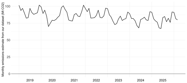
Monthly-updated territorial fossil CO2 emissions estimates for Japan
Taro Kunimitsu

Robbie M. Andrew
We present a low-lag, monthly dataset of emissions of carbon dioxide from fossil fuel consumption and industrial processes in Japan, derived directly from official activity data and starting in 2007. Such estimates will be crucial for near-real-time monitoring of emissions and making swift policy responses accordingly. When aggregated, our estimates replicate the annual data published through the UNFCCC national inventory report very well, with only small discrepancies which we describe and quantify. The dataset is produced with a lag of 2 months and can be used to estimate the annual emissions a year ahead of the official estimates submitted to the UNFCCC, and also provides a better starting point for short-term emissions projections. Data are available at https://doi.org/10.5281/zenodo.20023226 (Kunimitsu and Andrew, 2026).
- Article
(4956 KB) - Full-text XML
- BibTeX
- EndNote


1.1 Aim of constructing monthly emissions data
To meet the Paris Agreement goals on climate change, countries need to reduce their CO2 emissions. Measurement and monitoring are primary tools to facilitate such reductions. A growing number of countries publish annual estimates of their emissions, but these are typically published more than a year after the measurement year ends, and this delay can lead to missed opportunities for policy correction. Moreover, an annual temporal resolution hinders interpretation of emissions trends and reduces the potential frequency of raising awareness in society. Economic data are published quarterly, monthly, and at even higher frequencies precisely because this is required for steering economic decisions. Annual emissions reporting was reasonable in a time when they were less important, but as the world approaches 1.5 °C, closer monitoring of emissions is increasingly critical. There is therefore a clear policy need for emissions estimates that have both lower lag and higher temporal resolution.
In addition to the added value for policy correction and awareness raising, reliable sub-annual estimates will become comparison points for methods that rely on proxy parameters that are not country-specific (e.g. Liu et al., 2020), used in calibrations of satellite observation data (e.g. Chevallier, 2021), as well as for global short-term projections of CO2 (Friedlingstein et al., 2026).
As the world's fifth-largest emitter, Japan's emissions estimates are of interest not just domestically, but also to the international public. Japan has submitted its Nationally Determined Contribution (NDC) with targets of a 46 % decrease in greenhouse gas emissions by 2030 compared to 2013 levels, a 60 % decrease by 2035, a 73 % decrease by 2040, and net zero by 2050 (Japanese Government, 2021, 2025), all of which require policy measures informed by timely data. While many statistics in Japan are relatively well maintained at monthly resolution, no official estimates of sub-annual emissions are yet produced. Moreover, Japan's earliest report of annual emissions is published 12 months after the fiscal year has passed.
A monthly dataset specific to Japan is additionally useful because of the use of fiscal years in Japanese data: Japanese annual data on emissions are published for fiscal years, running from April to March the following year. When aggregating annual data with data from other countries, calendar-year values should be used for correct alignment, and while sometimes simple – allocations are made, monthly data offer a much more accurate reconstruction. A small number of other countries also report internationally on years other than the calendar year, such as Australia (Australian Government, 2025), Egypt (Egyptian Government, 2025), and Pakistan (Pakistani Government, 2025).
In this paper, we construct a dataset of monthly fossil CO2 emissions for the territory of Japan, derived from officially published national datasets. Compiling monthly emissions from the many datasets requires organization and conversion of existing statistics, as well as development of a deeper understanding of the derivation of current annual emissions estimates. The resulting dataset can readily be updated monthly as new source data are published.
1.2 Overview of public emissions data based on annual data
In line with the Paris Agreement, the Japanese government submits a highly detailed annual National Inventory Report (NIR) of anthropogenic emissions by sources and removals by sinks of greenhouse gasses (GHGs) to the United Nations Framework Convention on Climate Change (UNFCCC) secretariat (Greenhouse Gas Inventory Office of Japan and Ministry of the Environment, Japan, 2025). The report follows methods outlined in the 2006 IPCC Guidelines (Eggleston et al., 2006) and its updates (Calvo Buendia et al., 2019), and is revised and updated for every submission. For Japan, the report is created by the National Institute for Environmental Studies (NIES), under the supervision of the Ministry of Environment. The NIR is composed of two parts: the data are presented in the Common Reporting Tables (CRT), and the details in the National Inventory Document (NID). We will use the acronyms NIR, CRT, and NID throughout the paper.
Separately, the Agency for Natural Resources and Energy (ANRE) under the Ministry for Economy, Trade and Industry (METI) publishes the General Energy Statistics (METI, 2025, also sometimes referred to in English translations as the “Comprehensive Energy Statistics”) , which accompanies the Energy Supply and Demand Report. A preliminary edition is published annually in November of the year following the reported period, while the final edition is published in the subsequent April, usually coincident with the NIR submissions to the UNFCCC.
The Japanese government coordinates internally for the NIR submission to the UNFCCC and domestic publications from METI, so the data are mostly aligned, but there are some clear discrepancies due to differing category definitions and data sources. Following careful comparisons and consultation with the authorities, we have resolved the differences where data are available to the public. The data sources are summarized in Sect. 2.4, and relevant points are detailed for each fuel type or product in Appendix A.
1.3 Literature on sub-annual emissions estimates
The literature on sub-annual, especially on monthly, emissions estimates for individual countries, both from official sources and third-parties, was recently summarized by Andrew (2021), in his presentation of monthly emissions estimates for the European Union. We build on this summary focusing on relevance to our study and adding more recent additions to the space.
Countries where monthly data are published officially by the government include the United States, likely the first such case published in 2009 (EIA, 2009). Quarterly estimates are available for all EU countries (Eurostat, 2026), although these are not territorial emissions but rather estimates of emissions associated with the economic activity of each country, and these can diverge significantly (Andrew, 2021; see Appendix G for an example of divergence). In addition, Thailand's Ministry of Energy publishes detailed monthly energy data and derived energy-related, territorial CO2 emissions estimates with a lag of 6–8 weeks (Energy Policy and Planning Office, Ministry of Energy, Thailand, 2026), while Australia (Department of Climate Change, Energy, the Environment and Water, Australian Government, 2025), the United Kingdom (Office for National Statistics, UK Government, 2026) and New Zealand (Stats NZ, New Zealand Government, 2026) all publish quarterly territorial emissions estimates. France publishes monthly emissions estimates, published quarterly (Citepa, 2026). These are generally published around 3–5 months after the end of the quarter. Finally, South Korea began publishing quarterly estimates of emissions in its energy sector in late 2025 (Greenhouse Gas Inventory & Research Center of Korea, 2025), probably based on earlier work by Min and Choi (2024).
Third-party estimates also have a long history, with an early example from Blasing et al. (2005) for emissions from the consumption of fossil fuels in the United States for the period 1981–2002. Estimates based on actual activity statistics (as with the current study) have been created for individual countries by Gregg et al. (2008) for China, Andrew (2020b) for India, and Andrew (2021) for the European Union.
Andres et al. (2011) used methods based on proxy data developed by Gregg and Andres (2008) to estimate monthly emissions for 21 high-emitting countries and then map these to similar countries. Japan is among the 21 countries with direct estimates of emissions. The data source is confined to sales data of fossil fuels.
Several monthly emission datasets are available using sources other than activity statistics.
Oda and Maksyutov (2011) introduced the ODIAC dataset, which derives global, gridded emissions from national totals and satellite-derived night-light data. However, it was not until Oda et al. (2018) that sub-annual estimates were introduced, using the temporal profiles developed by Andres et al. (2011). With the advent of the COVID-19 pandemic, ODIAC's method for disaggregating annual emissions to monthly resolution has changed (Maksyutov and Oda, 2025, see Sect. 3.6.4), although this change doesn't appear to have been documented yet. The dataset is updated annually.
The EDGAR dataset (Emissions Database for Global Atmospheric Research) is the European Commission's in-house dataset. Having originally used IEA energy data to derive energy-related CO2 emissions following the IPCC Guidelines Tier-1 approach, EDGAR has since 2022 taken these directly from the IEA (European Commission Joint Research Centre, 2022) and supplemented with emissions in other sectors. EDGAR's dataset has been disaggregated to monthly resolution by the use of “temporal profiles”, which are a framework such that each sector's emissions can (but does not necessarily) vary each month and that this monthly profile can vary by year (Crippa et al., 2020).
During the early stages of the COVID-19 pandemic in 2020 it became clear that there was a need for estimates of global emissions at a higher temporal resolution and lower lag, and this led to the development of two new datasets using proxies to estimate emissions less directly (Le Quéré et al., 2020; Liu et al., 2020). The proxy approach relies on data that alone do not allow direct derivation of emissions, but when combined with an emissions baseline the relative changes in the proxy data can indicate changes in activity and therefore changes in emissions. They are proxy in the sense that they stand in for real activity data (e.g., traffic congestion stands in for gasoline consumption).
The work of Le Quéré et al. (2020) was largely driven by country-level data on the level of containment (restrictions on movement) and aggregated location data newly released by the technology companies Google and Apple as a part of pandemic response, and showed an average peak reduction in country-level emissions of 26 % at the height of the first lockdowns in early 2020. The purpose of this work was specifically to quantify the effects of the pandemic on emissions, and the proxy sources used are less suitable for more normal periods.
Liu et al. (2020) developed a dataset, known as Carbon Monitor, that also used changes in proxy indicators to produce estimates of relative changes from a baseline. The baseline in this case was EDGAR's estimates of emissions for 2018. Liu et al. divided up emissions in top-emitting countries into six sectors and used a separate proxy for each sector. The ability of these proxies to reflect actual changes in activity varied. In the power sector, for example, actual electricity generation data served as a relatively strong proxy, although initially only total generation was used, ignoring changes in generation mix, and initially only for a small number of countries. In contrast, the proxy used for road transport was a model of vehicle emissions as a function of an urban traffic congestion index in Paris, and this Parisian model was applied out of sample to several hundred cities around the world. Carbon Monitor has daily resolution, although some of the proxies used were only monthly. Liu et al.'s work continues to be updated approximately monthly, with a lag of about 2 months.
Oda et al. (2021) presented estimates of emissions from Japan's road transportation sector using official fuel consumption survey data and compared these with those of Carbon Monitor, finding that the latter's methods were inaccurate, failing to capture seasonal patterns of transport emissions. However, the authors recommend that research on using “unconventional activity data” (i.e. proxy data) continue.
In 2020, Climate TRACE was announced as a collaboration of nine climate and technology organizations (Worland, 2020) and released its first emissions estimates in 2021 (Climate TRACE, 2021). The method is described as being primarily based on “direct, independent observations”. The methods used for different sectors differ significantly. For example, in the power sector, emissions are estimated by deriving utilization factors for power plants using automated detection of water-vapor plumes from satellite imagery, combined with a database on power plant capacity and technology (Couture et al., 2024). Meanwhile, in the oil and gas sector, a detailed bottom-up model is used to estimate emissions at each facility, with very high data requirements. Some sectors, however, are simply extrapolated from the EDGAR global emissions dataset. Being largely untied to other emissions or fuel-consumption datasets, Climate TRACE's estimates in some cases currently deviate substantially from other estimates (e.g., Gurney et al., 2024, 2026). The dataset continues to be updated, with a lag of about 2 months.
The REAS dataset (Kurokawa and Ohara, 2020) includes monthly, gridded emissions estimates for East, Southeast, and South Asia. In general, monthly emissions are estimated by applying proxies to annual estimates, and for years in which monthly proxies are not available, extrapolations of sub-annual patterns are used. REAS is also incorporated into other, regional datasets such as MIXv2 (Li et al., 2024) and CoCO2-MOSAIC (Urraca et al., 2024).
The MEIC-global-CO2 dataset (Xu et al., 2024) provides monthly emissions estimates from 208 countries/territories for 1970–2024, although we could not find documentation on the methodology behind its monthly data construction.
Local city-level data have been compiled at the monthly level, including for Japanese cities. One study is for Tokyo, using ground-based measurements of CO2 (Ohyama et al., 2023). While feasible at local level, where such measurements are available as constraints, this method cannot readily be extended to the whole country.
While some estimates of Japan's sub-annual territorial emissions are available, it is clear there is a need for low-lag estimates that are grounded in official data. The current study focuses on official energy consumption and production statistics, which aligns better with established methods (Eggleston et al., 2006).
2.1 Goal of analysis
We aim to construct a dataset of territorial CO2 emissions from fossil fuel sources and industrial processes (combined, these are called “fossil CO2” by the Global Carbon Project; Friedlingstein et al., 2026), covering the majority of Japan's emissions, with sub-annual temporal resolution and low lag, using monthly activity data published by the Japanese government. We then use this monthly dataset to construct an annual emissions estimate for the latest full fiscal year (April 2025 to March 2026), which is not yet available from official sources, as well as historical calendar-year estimates, which the Japanese government does not publish.
We take the reference approach (see Sect. 2.2) for fossil fuels, mainly using the energy supply data and not looking into sectoral usage (except for non-energy usage, especially for secondary fuels). This approach has significantly lower data requirements compared to the sectoral approach, in which the emissions from combustion are tracked for each sector individually at a high level of detail. The sectoral approach is the official method used to estimate annual emissions in the NIR, while the reference approach is intended as a cross-check. We compare these in Sect. 2.2 to justify our use of the reference approach.
Emissions associated with fossil fuels occur at the time of consumption, when the carbon in the fuel is oxidized, and monthly data on fuel consumption are therefore preferred, but they are not always available. However, Japan has very limited domestic resources and therefore imports a very large proportion of its fossil fuel input, so monthly trade data become an invaluable source of information. We use reported consumption where available and supplement this with net-import data where necessary, assuming that changes in domestic stocks of the fuels are relatively stable over time in Japan when data are not available.
As a necessary step to confirm that our choice of monthly data is appropriate and sufficient for our purposes, we attempt to replicate the annual reference approach data submitted to the UNFCCC in the NIR, effectively designating this as the ground truth, recognizing the very significant effort put into its elaboration and revision over many years, following established methodologies, and including international auditing processes under the UNFCCC (UNFCCC, 2015).
Our dataset includes all the largest sources of emissions and the most important minor sources, accounting for about 99 % of total emissions in 2023. That is, the omitted sources account for about 1 % of total emissions in 2023. We omit these minor sources due to a lack of available monthly data, but we may revisit these in future revisions of the dataset. For fossil fuels, we include most primary and secondary categories included in the CRT; these are listed in Sect. 2.4 and detailed in Appendix A. In addition to fossil fuels, we include three major categories of carbonate decomposition in the IPCC-defined Industrial Processes and Product Use sector, namely cement production, lime production, and the use of limestone in the production of pig iron.
Directly related to energy usage are emissions from waste incineration and biomass usage. For waste, which is composed of products derived from both fossil fuels and biomass, we include the monthly data reconstructed from annual data (see Appendix A). For use of biomass as an unadulterated energy source, the NIR does not directly include these in the total emissions to avoid double counting, since any net emissions from biomass combustion are reported under the land use, land-use change and forestry (LULUCF) sector, so we also exclude this accordingly.
There are other categories included in the NIR that we do not include in this analysis. We do not include agricultural CO2 emissions (arising from the application of urea and lime), since in Japan these emissions are negligible compared to the other sectors discussed and data are limited. We also exclude emissions in the LULUCF sector, which have very different accounting and modelling approaches, and are outside the scope of our dataset, which focuses on emissions of CO2 from fossil sources, aligning with the scope of the EFOS term of the Global Carbon Budget (Friedlingstein et al., 2026).
2.2 Reference approach vs sectoral approach
For estimating emissions from the oxidation of fossil fuels, we use the reference approach, which is derived from the country's apparent total fuel consumption. Apparent consumption is the net supply of fuel energy within the territory, defined for primary fuels as (Eggleston et al., 2006):
For secondary fuels, the production term should be dropped since this is already accounted for in primary fuels. The International bunkers term represents fuels supplied by the country but used for international transportation, which is excluded from territorial emissions estimates.
The reason this is called “apparent” consumption is to contrast with actual measured consumption, which might be available through full sampling of all users, but generally is not. The difference between the two is not only differences in statistics (e.g., missing information), but also the coverage of the term “Stock Change”, which often does not include changes in all categories of stock, especially tertiary (see Sect. 3.5.2).
As described in Sect. 2.1, the sectoral approach provides the official estimates of emissions in the NIR, while the reference approach is primarily used for verification purposes. While detailed sectoral usage data are only available at annual resolution, impeding our ability to estimate emissions via the sectoral approach at monthly resolution, the data required to produce reference-approach estimates at monthly resolution are available. Further, as we will show, the two approaches largely agree in Japan's case. To build on the data published by the government on a monthly basis, it is therefore more practical and natural to use the reference approach.
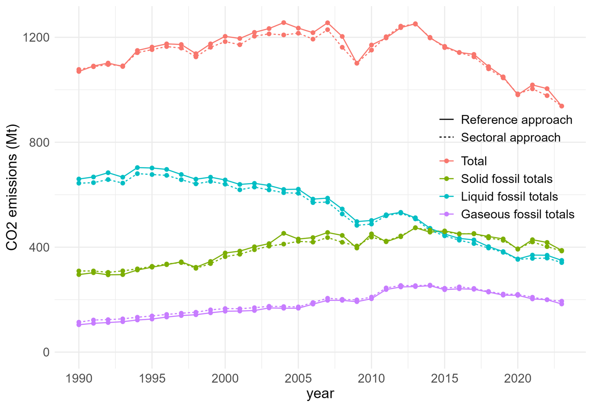
Figure 1Comparison of officially reported emissions using the reference approach and the sectoral approach reported in the CRT (Greenhouse Gas Inventory Office of Japan and Ministry of the Environment, Japan, 2025).
In determining the total emissions, non-energy usage of fuels must be subtracted from apparent consumption as defined above, since a large part of this use does not lead to oxidized carbon and therefore CO2 emissions.1 Determining the amount of non-energy usage generally requires some data from individual sectoral usage (see Appendix A for further details).
The differences between the values from the two approaches for fuel combustion are shown in Fig. 1, and are also summarized in the NID, showing a maximum difference of 4 % in 2004, but generally smaller than 1 %. Individual fuels can show larger discrepancies in single years, up to 10 % for solid fuels in 2004, which is due to differing calorific values after product transformation, among other reasons.
The small differences in the values of the two methods are not a universal property globally. Norway, for example, has a large discrepancy between the two approaches – more than 50 % in the year 2000 – due to the large production and export of oil and gas, resulting in large statistical discrepancy in the residual domestic consumption (Norwegian Government (2025), see Appendix K). Japan imports almost all its fossil fuel resources, so is structurally robust to this type of discrepancy.
2.3 Conversion factors
Two conversion factors are needed to convert consumption and production values of fossil fuels (either weight or volume) into carbon emissions: the calorific value (also known as energy content), and the emission factor.
The calorific value is defined as the amount of heat generated from the combustion of the fuel. All statistics in this analysis (and from the Japanese government) use Gross Calorific Values (GCVs), which include the energy after water vapor produced during combustion is condensed and the heat recovered, so-called latent heat. This contrasts with the lower Net Calorific Values (NCVs), which exclude the latent heat amount (Eggleston et al., 2006). While the IPCC guidelines use NCVs as the default, they are derived from GCVs, and they are most often converted from one to the other using simple constant factors.
The other conversion factor is the carbon emission factor: how much carbon is produced per unit energy. The annual domestic reporting from ANRE provides the amount of carbon instead of CO2, so the carbon emission factors are defined for carbon accordingly. We convert this factor to a CO2 conversion factor by multiplying , the ratio of the molecular mass of carbon dioxide and a carbon atom, to recover the amount of CO2 emitted. The factor does not consider isotopes of carbon and oxygen, but the IPCC guidelines and the NIR from Japan both explicitly employ the factor for calculations for simplicity, so for our replication purposes here we also use this. We also assume that all input carbon is fully oxidized through to CO2 (that is, the Carbon Oxidation Factor (COF) is 1, implying highest level of combustion efficiency), in line with the assumptions in Japan's NIR based on measurements and industry hearings.
METI determines standard values for both the GCV and emission factors, which are revised about every 5 years. While these are set for default reference, changes in fuels and technology, such as the composition of the fuels, shift the actual energy and carbon contents every year (and, indeed, every month). Thus, METI also uses measured factors (“actual” values) for some fuels in their annual reporting. The NIR also uses these actual factors where applicable, rather than the domestic reference values or the IPCC 2006 guideline default values. We use these measured values for our emissions estimates and use the latest available value to extrapolate to the current year.
For the production of cement, lime, and pig iron, one conversion factor that converts directly from production amount to emissions is used. We also detail these in the following section.
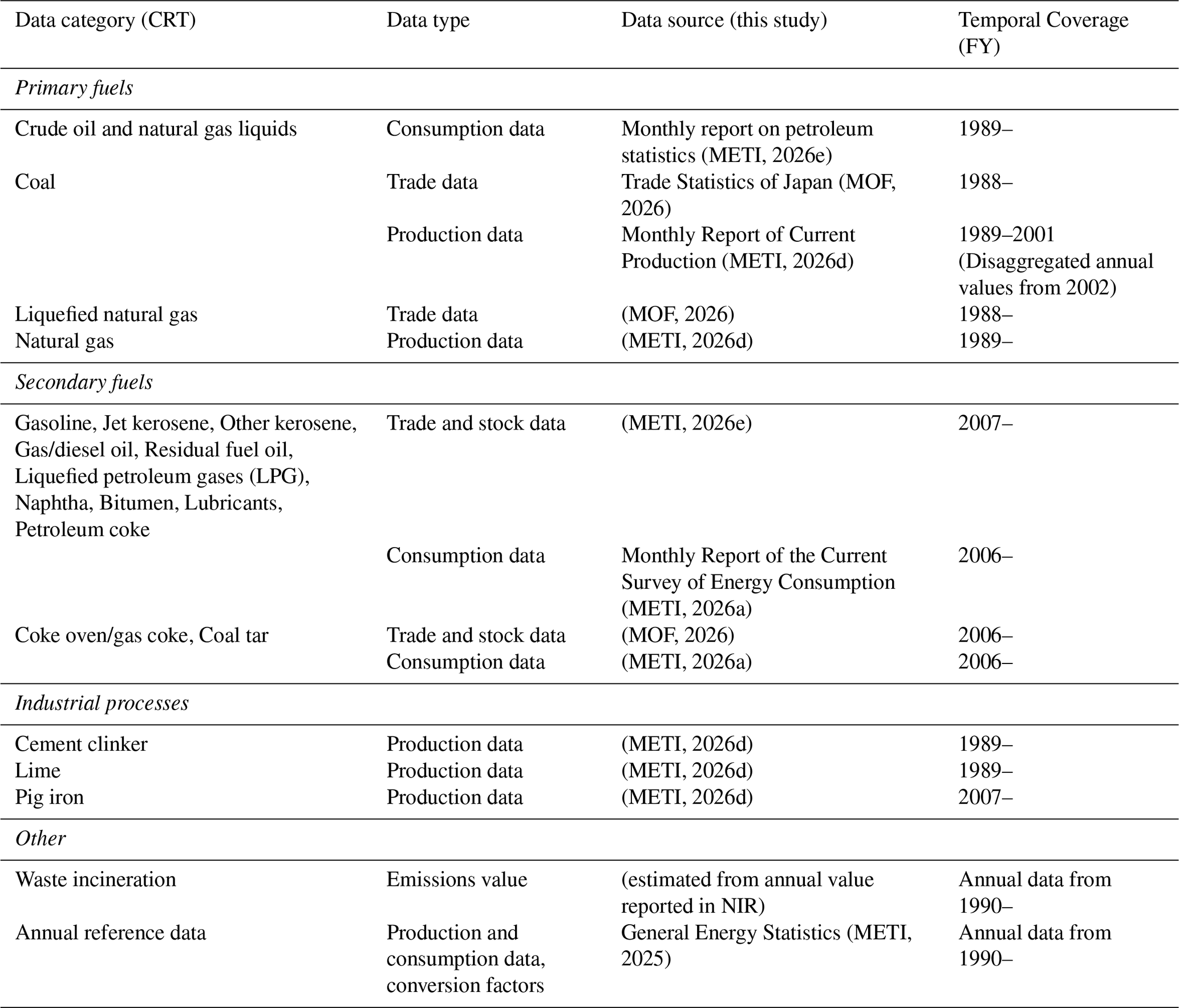
2.4 Description of data
Table 1 summarizes the main characteristics of the monthly data for each of the fossil fuels and industrial processes, including the temporal coverage. While temporal coverage differs for different emission sources, 2007 and onwards is covered for all sources considered in this study.
Most annual data published by the Japanese government (including the NIR submission) is based on the Japanese fiscal year (FY), i.e. from April of the stated year to March the following year. For example, FY2023 represents the period from April 2023 to March 2024. While this does not directly affect monthly data, this must be borne in mind for the reconstruction of and comparison with annual data.
For a detailed description of the sources and adjustments conducted, see Appendix A.
In this section, we present the monthly CO2 emissions estimates aggregated into annual values for each fuel type and industrial process, and compare these to the CRT values submitted to the UNFCCC with possible explanations of any discrepancies. For fossil fuels, we aggregate the monthly data by the three fuel types, liquid fossil fuel (oil and oil-based products; this category also includes NGL), solid fossil fuel (coal and coal-based products), and gaseous fossil fuel (liquefied natural gas and domestically produced natural gas; note that this category does not include oil-derived gaseous fuels, e.g. LPG).
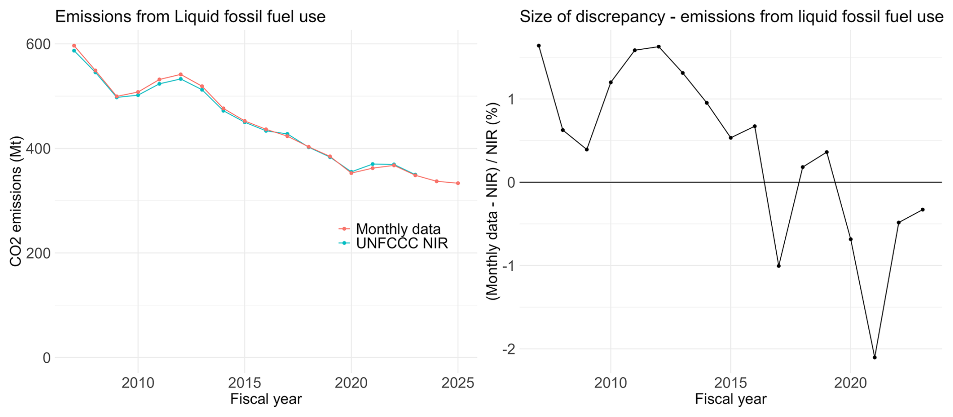
Figure 2Liquid fossil fuel emissions comparison of aggregated monthly data (including FY 2025 estimates) and UNFCCC NIR data.
3.1 Emissions from individual sources
For liquid fossil fuels (Fig. 2), including crude oil and fuel products, we obtain a relatively accurate replication for recent years (below 2 % deviation except 2021) between NIR data and aggregated monthly statistics based on data as explained in Sect. 2.4.
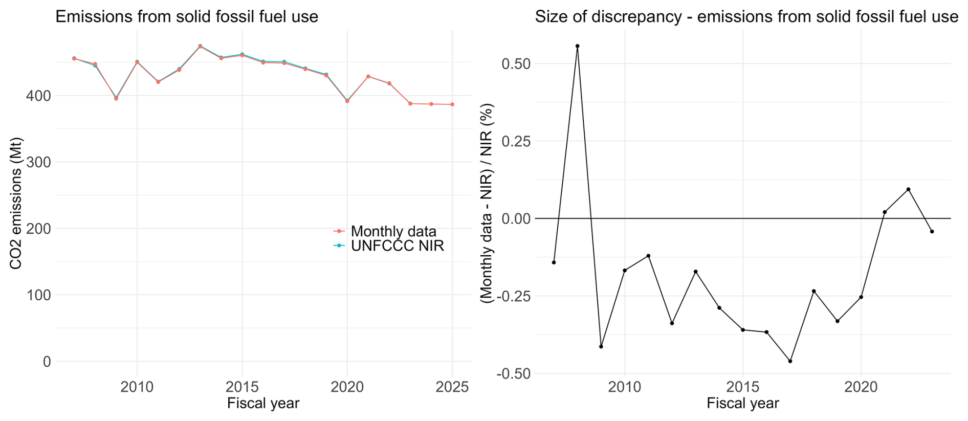
Figure 3Solid fossil fuel emissions comparison of aggregated monthly data (including FY 2025 estimates) and UNFCCC NIR data.
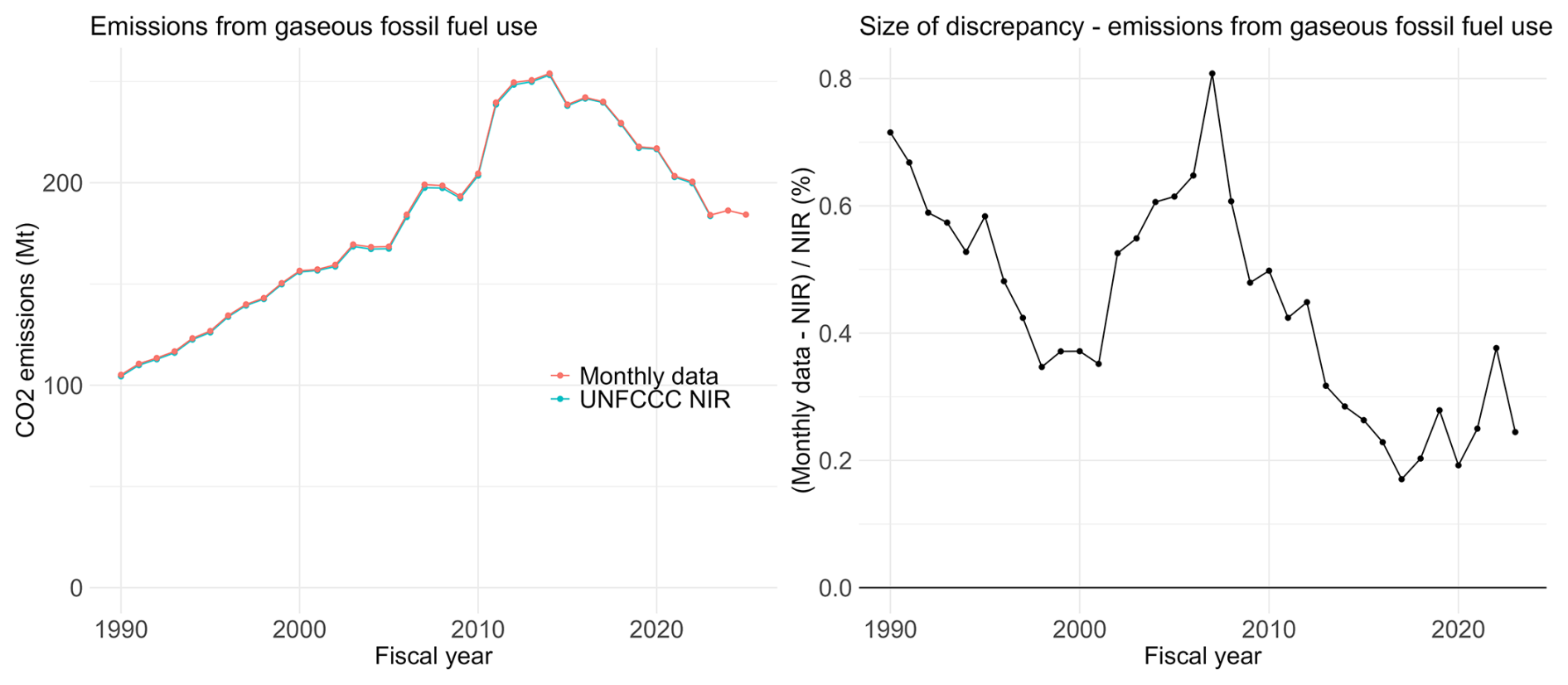
Figure 4Gaseous fossil fuel emissions comparison of aggregated monthly data (including FY 2025 estimates) and UNFCCC NIR data.
Monthly data on the total consumption of coal and coal-based products (Fig. 3) reproduces the annual emission data well (maximum discrepancy of 1.1 %), but with slightly lower values in most years.
The monthly natural gas data (sum of import and domestic production) combined with measured conversion factors replicate the CRT values very precisely, with a maximum discrepancy of 0.8 % throughout the period with available data (Fig. 4). There is a small systematic overestimation for emission which is likely due to the non-energy usage of natural gas not being excluded from our estimates. While monthly data for this non-energy use are available, a large portion of this (75 % for FY 2023) still results in emission of CO2 in the ammonia industry through the use of resulting urea, among others, so there is a cancellation effect when considering the total emissions. We do not include ammonia production emissions and other non-energy use processes of natural gas in this study due to the lack of detailed data, so we do not subtract the non-energy usage amount from the total emissions here.
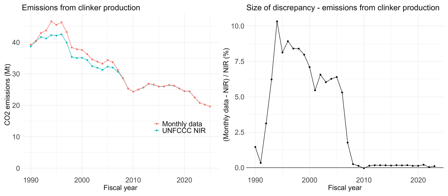
Figure 5Cement production emissions comparison of aggregated monthly data (including FY 2025 estimates) and UNFCCC NIR data.
For cement production (Fig. 5), the amount of clinker produced is directly converted to emissions with one emission factor, which we take from the NIR for both the monthly METI data and UNFCCC annual data.
For recent years, the monthly data published by METI matches very well with the annual values reported to UNFCCC, with less than 0.3 % discrepancy from 2008. The discrepancy in the early years of data may come from the difference in data source: the values reported to the UNFCCC are based on data provided to NIES by the Japan Cement Association, while the monthly values from METI are based on direct surveys of cement companies. While these differences may have led to coverage differences, current production statistics that are available from the Japan Cement Association (Japan Cement Association, 2026) do not match those in the NIR during this period. In contrast, they are in line with the domestic annual values reported by METI. This discrepancy will distort the monthly statistics in these earlier years, but for recent years, the difference is small enough to give confidence in the monthly values.
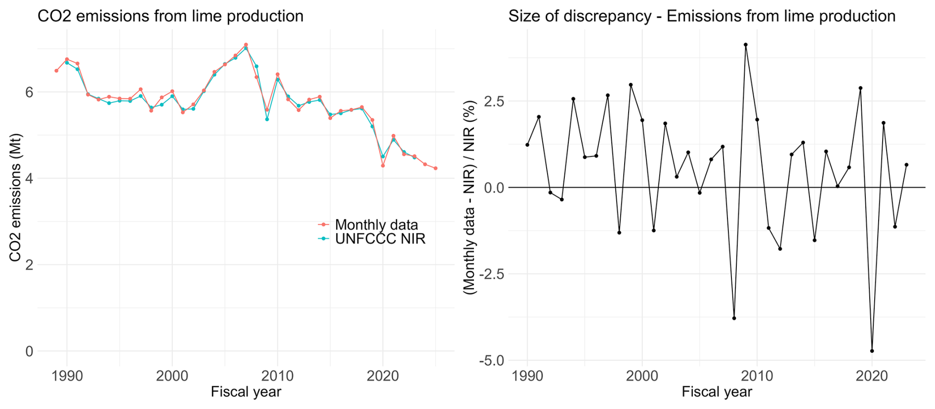
Figure 6Lime production emissions comparison of aggregated monthly data (including FY 2025 estimates) and UNFCCC NIR data.
We reconstruct the annual emissions data using monthly quick lime production data, resulting in values within 5 % of the annual data for all years (Fig. 6). There is no systematic bias in the discrepancy between the two values, and the trends follow each other. Given that the two estimates are derived from two different sets of activity data (limestone consumption for NIR, quick lime production for monthly data), and that lime is a relatively minor category within the overall emissions, the match is sufficient for our purposes.
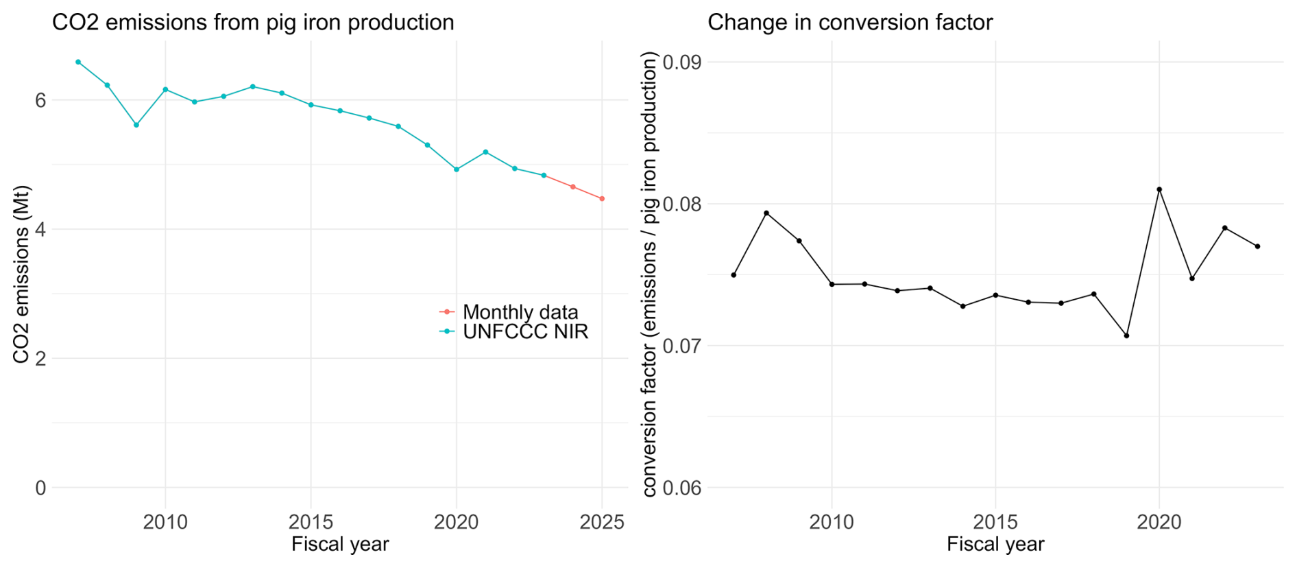
Figure 7Pig iron production emission comparison of aggregated monthly data (including FY 2025 estimates) and UNFCCC NIR data.
The monthly values for emissions from the decomposition of carbonates in the production of pig iron (Fig. 7) are estimated by proportional disaggregation of the annual value, so the reconstruction of emissions in this category matches exactly with the values reported in the UNFCCC NIR by definition. Our estimates for 2024 and 2025 are extrapolated using the 2023 conversion factor. The figure to the right shows how the ratio of CO2 emissions to pig iron production has changed throughout the period. While the year-to-year variations are accounted for within each year given our estimation method, the larger variation in recent years shows that there are possibly within-year variations of the same order as monthly production variations, at a few percent. Emissions in this category are relatively minor within overall emissions, so applying a constant conversion factor within the fiscal year and the extrapolating the conversion factor from 2023 to later years is sufficient for our purposes, while acknowledging the uncertainties.
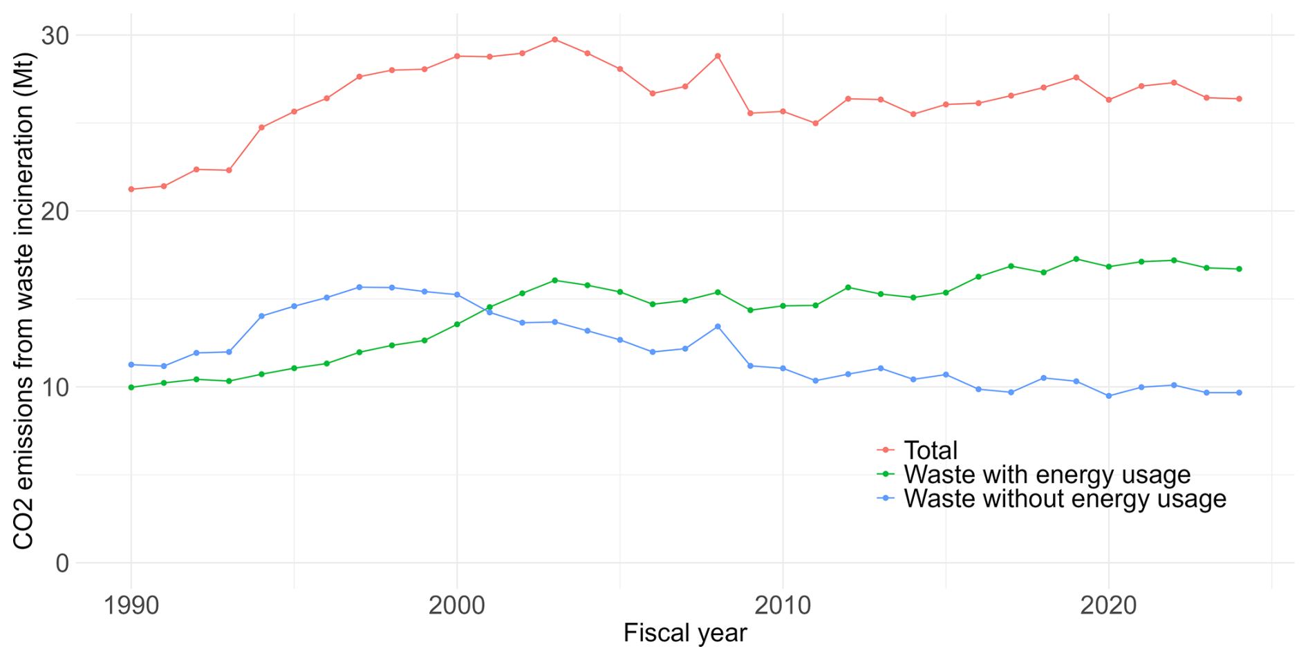
For waste incineration (Fig. 8), we divide the annual statistics reported in the NIR into months by a linear scaling (see Appendix B). In the NIR, emissions are divided into those that accompany energy usage and those that do not, so we keep this distinction, but also show the total value in Fig. 8. Observing that emissions have been relatively flat in recent years, we set the value for 2024 to be the same as that for 2023.
3.2 Total emissions and FY 2025 estimate
Summing over the monthly emissions in the Energy sector obtained in this study (fossil fuel emissions, including from waste incinerated for energy use), we obtain a total value within 1 % of the total annual reference value emissions reported in the CRT for all years 2007–2023.
For emissions from the Industrial Processes and Product Use sector, the three categories we estimate (cement, lime, and pig iron production) fall again within 1 % of the total annual value of these three categories reported in the CRT for all years 2007–2023. In turn, these three add up to approximately 78 % of the total emissions of the whole category. The category total is in turn around 4 % of emissions from the fossil fuel above. Hence, the missing amount (e.g. emissions coming from carbonates decomposed in glass and ceramic production) is below 1 % of the two categories combined.
The official annual emissions estimate for FY 2025 has not been published by the Japanese government at the time of writing, nor submitted to the UNFCCC, and both are expected to be released in April 2027. We can estimate the total annual emissions for FY 2025 by summing up the monthly estimates that we have compiled, given the expected differences with the official reported values discussed above. The total emissions for the sum of the energy sector, industrial processes and product use sector, and waste sector (including incineration not used for energy) using this method is estimated to be 958 Mt CO2, a 0.7 % decrease from FY 2024. Uncertainties are discussed in Sect. 3.5.
Calendar year (CY) estimates can also be trivially derived from the same compiled monthly dataset. CY 2025 emissions are estimated to be 1.0 % lower than CY 2024.
Assuming that the Japanese government continues to publish according to recent schedules, we will be able to estimate FY 2026 (the period April 2026 through March 2027) in May 2027.
3.3 Scaling of emission estimates
While our estimated total emissions are, when aggregated, very close to the officially reported annual values as discussed in Sect. 3.2, we expect the monthly values to be more accurate by scaling the values so that the sums add up to the official annual total estimates, i.e. those reported in the NIR.
For each category described in Sect. 3.1, we scale the monthly values to match the annual category total in the NIR. For FY 2024 and 2025, which are beyond the reference NIR year, we use the same scaling factor as FY 2023 for all categories.
For our final monthly estimates, we report these scaled monthly values per category as our primary monthly estimate, and also supplement this with the scaled monthly values of subcategories.
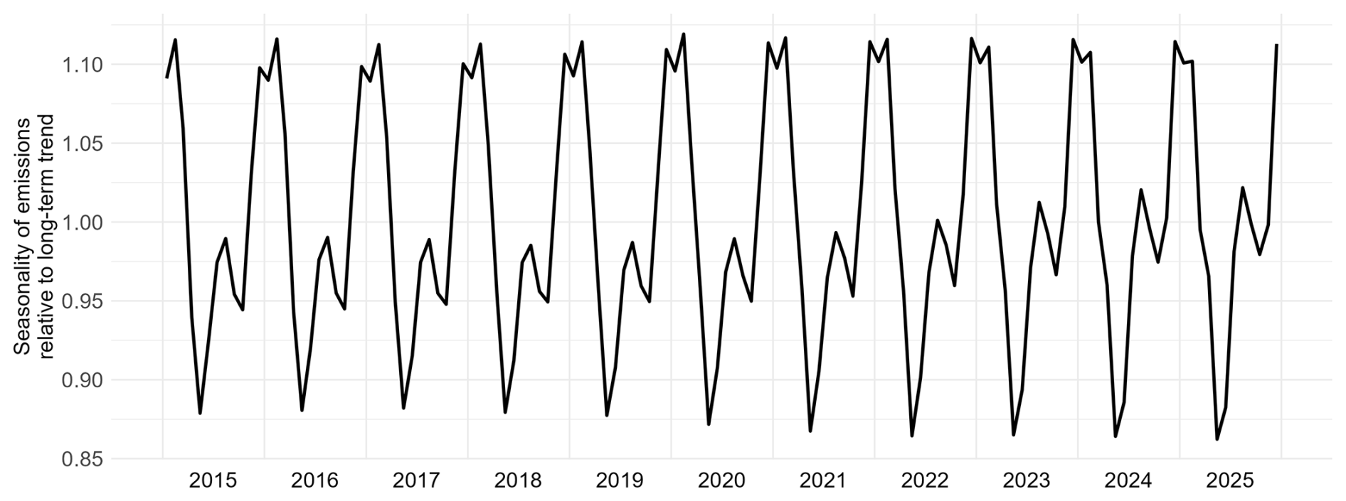
Figure 9Seasonal element of monthly emissions estimate, based on the X-11 method. Values are with respect to the underlying trend and adjusted for days in month.
3.4 Seasonality of emission estimates
To understand the monthly estimates we obtained, we present the seasonality patterns using the seasonal element obtained through the X-11 method (see Eurostat, 2013 and Appendix J). The X-11 method is a commonly used seasonal adjustment method which decomposes the data into its trend, seasonal, and irregular components. The decomposition captures large-scale behavior in the first two components, while all the remaining elements, e.g. abrupt shocks such as COVID-19 lockdowns, are captured in the last component. Figure 9 shows the seasonal element of the monthly time series from this analysis, which is shown as a multiplicative factor of the underlying trend component. We use the multiplicative form here to show seasonality independent of changes in absolute emission levels.
The X-11 method intentionally smooths the data to identify seasonality, but this means that any abrupt, real changes in seasonality are not identified, and we must be cautious interpreting the rate of change of the seasonality component. We do, however, see a clear peak in the winter (December, January, and February) and a smaller peak in the summer (July and August). The small peak in summer has increased in the past 10 years, while the February peak has become relatively slightly smaller compared to December and January.
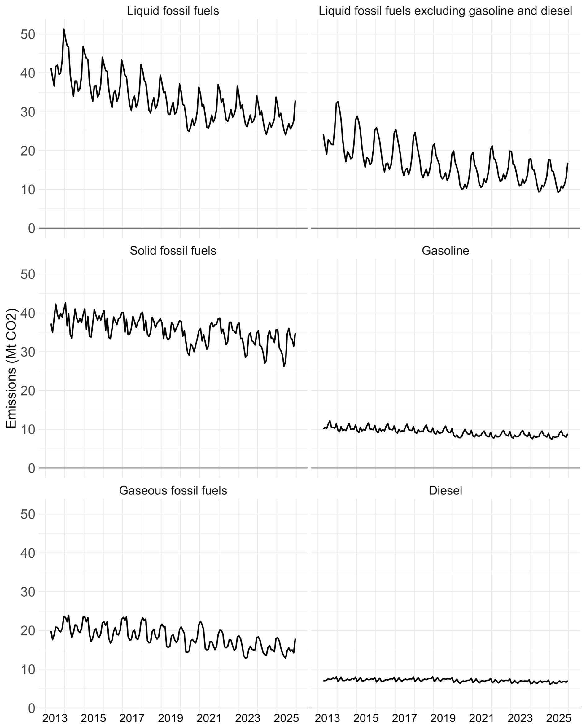
Figure 10Emissions seasonality and trend (excluding noise element) by fuel category, including gasoline and diesel data, and liquid fossil fuels excluding those.
To identify the drivers of this seasonality, we show in Fig. 10 the emissions trend and seasonality broken down by fossil fuel category. Here, we combine the trend and seasonality components to show the emission values of these components, to allow comparison between emission categories. In addition, we show liquid fossil fuels emissions subtracting out gasoline and diesel, along with gasoline and diesel separately. Gasoline and diesel are used primarily in the transport sector, and the separation allows us to see whether the seasonality is related to this sector. Note that these emissions of gasoline and diesel are derived separately from the METI sales data, and are not part of the overall monthly emissions data that we have created. This is the case since the reference approach does not contain direct information about the usage of secondary fuels, only the additional inputs and outputs to primary fuels.
We see that the large seasonality in the emissions mainly comes from Liquid fossil fuels, specifically from the sectors excluding gasoline and diesel. This means the seasonality is likely not coming from the transportation sector. While seasonality can potentially arise from the industry sector as well, we expect the seasonal element to be primarily originating from the residential and commercial sector use of liquid fossil fuels, where winter space heating is the main usage and would have strong seasonality.
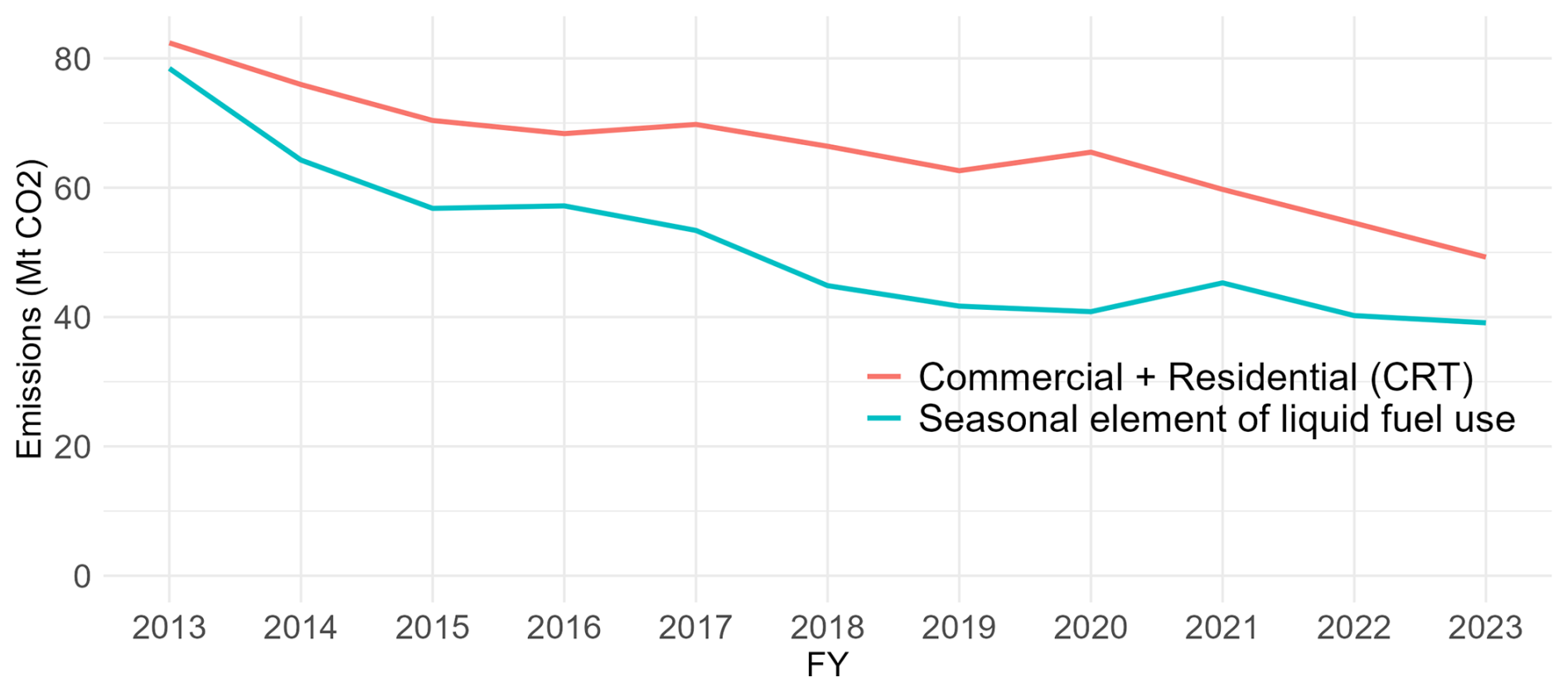
Figure 11Comparison of liquid fossil fuel emissions seasonal element and annual emissions from the commercial and residential sector.
To partially test the conclusion that the seasonality in the liquid fossil fuel emissions comes from the commercial and residential sectors, we take the simple approach of generating an approximate data series of the season-dependent non-transport liquid fossil-fuel emissions by subtracting the minimum monthly emission value each year from the monthly emissions for liquid fossil fuels excluding gasoline and diesel, and compare the annual aggregate to the emissions from the commercial and residential sector emissions obtained from the NIR. Figure 11 shows the comparison of the two values. While the values do not exactly match, the order and trend of the values are in line with each other, which supports the conclusion that the additional seasonal components mainly come from heating in the commercial and residential sectors.
There is also seasonality in the emissions from solid fossil fuel and gaseous fossil fuel. Solid fossil fuel emissions drop in the early summer, while gaseous fossil fuel emissions have a winter and summer peak similar to those of liquid fossil fuel. Solid fossil fuel is usually not directly used for space heating, only through electricity generation (around half of total solid fossil fuel emissions), which is one possible reason there is a less prominent winter peak, since coal-fired electricity is only part of the heating energy source. Gaseous fossil fuel is used similarly to liquid fossil fuel for heating in the commercial and residential sectors through electricity and distributed gas, explaining the similar seasonality. The size of the seasonal variation is smaller than that of liquid fossil fuel emissions for both, with average annual ranges (max-min) throughout the period of 11.0, 7.6, 6.0 Mt for liquid, solid, gaseous fossil fuel CO2 emissions, respectively.
3.5 Uncertainties in the emission estimates
Here, we list the uncertainties of the estimate that can make it diverge from the actual emissions, evaluate them where possible, and estimate the total uncertainty within our monthly data. We categorize the uncertainties into five groups: Uncertainty by category omission in this specific study, uncertainty from stocks, uncertainty present in the annual statistics, uncertainty coming from the use of monthly data, and uncertainty inherent in the reference approach.
3.5.1 Uncertainty by omission in this study
There are minor categories that are included in the NIR but that we excluded in this study due to lack of reliable monthly data. Categories missing in the energy sector include Refinery feedstocks, which are semi-finished oil products generated during the refining process, and “Other oil”, which are by-product gases in refining and petrochemical processes. The former is at most 0.5 % of total emissions, while the latter is much smaller and not reported in many years.
Categories missing in the Industrial processes and product use sector, adding up to 1 % of total emissions, include the incineration of non-methane volatile organic compounds (NMVOCs) – used for paints, printing solvents, cleansing, etc. – which comprise 0.2 % of total emissions; carbon black production, 0.1 %; ammonia production, 0.1 %; and smaller categories such as ceramics and glass production. Their monthly variations are expected to be much smaller than these proportions, so after scaling the total emissions to account for these missing categories, the impact on the monthly variation of the overall total will be negligible.
We keep the discrepancy due to omission as a contribution to the overall uncertainty, while as described in Sect. 3.2, we scale the aggregated values to match the annual total value to account for omissions and obtain a best estimate of the actual total.
3.5.2 Uncertainty from stock amount
We identify stock issues as the single most important factor specific to monthly emissions estimates when compared with annual estimates. Stocks are difficult to track, especially tertiary stocks described below, which lead to large uncertainties in estimates.
Even if the amount of stock is the same, the ratio of stock to usage in a certain period is larger for shorter time periods. Hence, its impact on monthly data uncertainty could become much larger compared to annual data uncertainty. The issue becomes larger when seasonality is taken into account, since the change in stock value is expected to be larger due to seasonal trends compared to interannual values at the same point of the year.
In addition to the officially documented stocks, tertiary stocks – stocks that are held by the end-consumers rather than the surveyable industry actors – lead to actual emissions not coinciding temporally with the sales recorded, and hence uncertainty in emissions that are not trackable by sector consumption data. This is of particular interest in the transport sector, where consumers can stock gasoline in their vehicles' fuel tanks. While we do not expect driving patterns on average to change dramatically in typical situations, this can become a significant factor for example in a COVID-19-like lockdown situation, where a consumer can fill their tanks in a certain month, but retain it there for several months with very few occasions of driving. Use of fuel sales data therefore results in a temporal displacement between estimated emissions and when those emissions actually occur. We do not quantify the uncertainties here due to lack of reliable methods for estimating, but note that more investigation of this issue may be warranted for emissions time series with high temporal resolution.
3.5.3 Uncertainty present in the annual statistics
Since data sources used in this study are mostly in line with those used in the official annual estimates, the uncertainties already present in the annual data are generally present in our monthly estimates. These include the lack of activity data for certain emissions sources and errors in activity measurements, among other sources (Greenhouse Gas Inventory Office of Japan and Ministry of the Environment, Japan, 2025). The largest uncertainty comes from the amount of coal consumed, where the statistical discrepancy between the input (supply-side data) and sectoral output (demand-side data) is large, especially for coke. The NIR estimates the uncertainty in total emissions to be at −3 % to +2 %, so we adopt these values.
The size of this uncertainty can also be inferred from revisions to annual data in later years. Annual values in the NIR are revised retrospectively with corrections and updated methods. For Japan, the revision level has been minor – within 2 % of total emissions – and especially after 2016, the change to past values have been below 0.4 % (Fig. I1). That is, despite many years of method development, revisions, and external auditing, changes have been very minor, and this gives confidence that also future revisions to our monthly estimates will be small.
Oxidization rate is another source of uncertainty, although as described in Sect. 2.3, the value is very close to 1 for all fuel use, and is set to 1 in official estimates. The NIR notes the possibility of up to 0.5 % non-oxidation for liquid fuels and 0.4 % for solid fuels, but quantitative data was not obtained for the former and the uncertainty is regarded small enough to be approximated as 0 in both cases.
3.5.4 Uncertainty coming from the use of monthly data
As described in Sect. 3.1, most monthly data sources exhibit some divergence from the annual data when aggregated to the same period. This can be the result of category omissions explained in Sect. 3.5.1, data source differences, or retrospective revisions, among other reasons. In some cases, very large discrepancies are found when the primary data comes from different sources, such as cement production before 2008, where the discrepancy between the monthly estimates and reference annual data becomes as large as 10 %. Such cases are not found for recent years, and we do not expect this to be an issue in data for future estimates. This can be thought of as the result of better reporting and methodological improvements over the years, leading to ever lower uncertainty in the estimates.
Taking the weighted sum of all the discrepancies in the annual reported value and aggregate value from monthly data from 2007 to 2023, where the discrepancies are calculated as root mean squared values, we obtain an upper bound uncertainty of 0.8 %. This is a conservative estimate since taking the sum overestimates correlation. This uncertainty is what is obtained from comparison to the annual value, and does not include uncertainties arising from monthly variance, for example coming from stock changes explained in Sect. 3.5.2.
One source of monthly uncertainty inherent in our method is the use of annual values without monthly data. While we scale all top-level categories to match the annual reported values, the monthly values for the following emission sources are all or partly determined to add up to the CRT annual values even before the scaling: Naphtha, Lubricants, Bitumen, Pig iron, Waste. The estimation of monthly values ranges from plausible process-based variation (Naphtha and Pig iron, although the latter has some uncertainty from the variation of the conversion factor as shown in Sect. 3.1) to no additional information beyond annual total (Lubricants, Bitumen, Waste). For the latter category, the monthly values are estimated using a linear disaggregation method (see Appendix B), which may potentially have large intrinsic uncertainties at the monthly level, but with very small contribution to overall emissions uncertainty. In addition, for these emissions sources, the latest years (FY 2024 and 2025) rely on values estimated from a previous year (FY 2023) for both activity amount and conversion factors, which again leads to discrepancies from the actual emissions value.
Retrospective corrections and updates
As with annual data, monthly data can be updated after a certain period from their publication. The relative size of the correction could potentially be larger than the annual version, since misreporting may be corrected more often within a shorter period. But retrospective monthly revisions that have been identified through revision datasets published by METI are minor.
3.5.5 Uncertainty inherent in the reference approach
As discussed in Sect. 2.1, the sectoral approach is the official annual estimation method for emissions, and the reference approach is only used for verification purposes in the NIR. This methodological difference has inherent sources of uncertainty. Points documented in the NID include the fact that not all energy use inputs are oxidized and that they may add to stocks within the sector; Changes in per unit energy emissions may also occur due to transformation into different products.
The size of this uncertainty can be roughly estimated from the difference between the values in the sectoral approach and the reference approach (Sect. 2.2), at around 1 % for most years. While the difference could be larger for monthly values, especially due to the lack of inventory data, we do not see large sources of difference other than those accounted for previously.
3.5.6 Total uncertainty estimate
On the reasonable assumption that the component uncertainties are mostly independent of each other, we take the square root of the sum of squares for the quantified uncertainties to estimate the total uncertainty. The overall uncertainty is dominated by that in coal consumption, already existing in the annual uncertainty analysis. The uncertainty for total emissions in each month is estimated to be ± 3 % at 2 standard deviations (95 % onfidence interval), given the uncertainties in the NIR are also given at 2 standard deviations. Note that this does not include the uncertainties that could not be quantified, such as those from tertiary stocks.
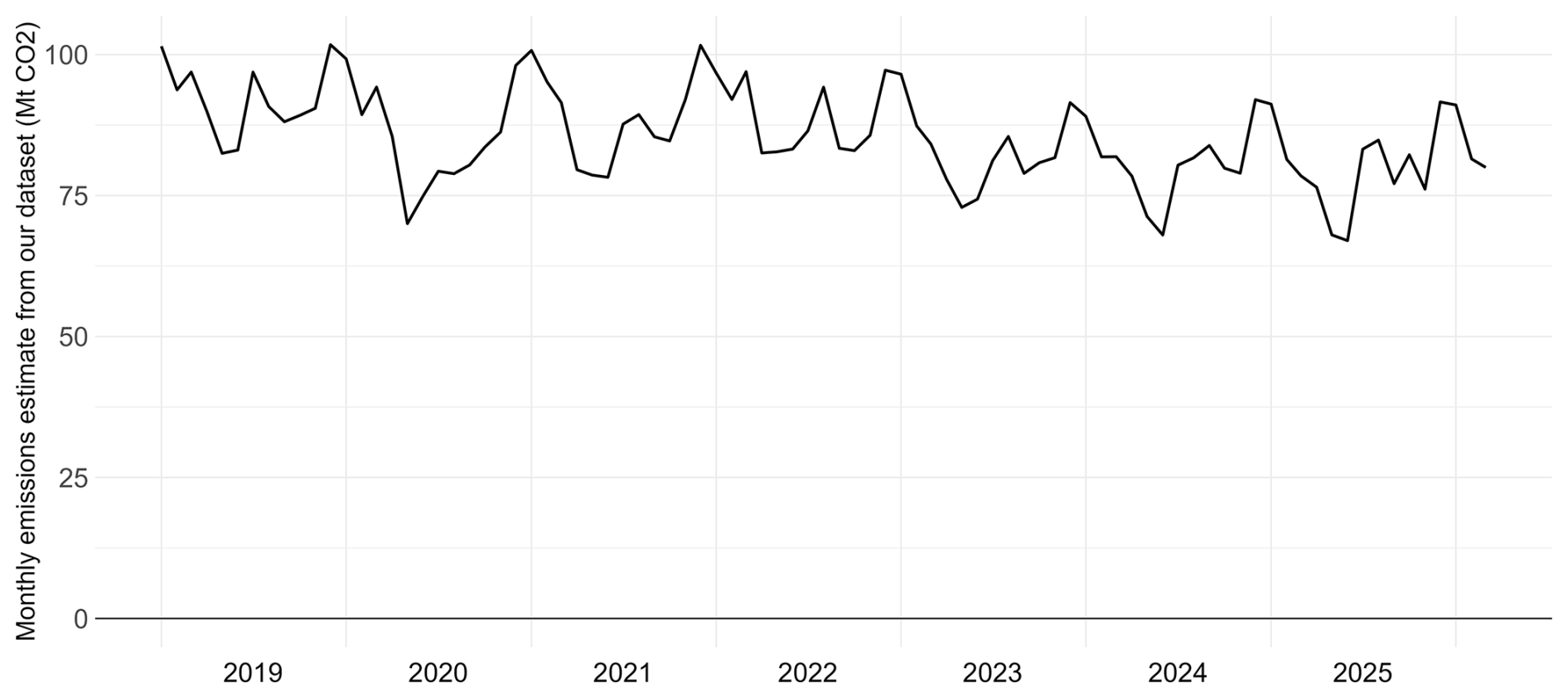
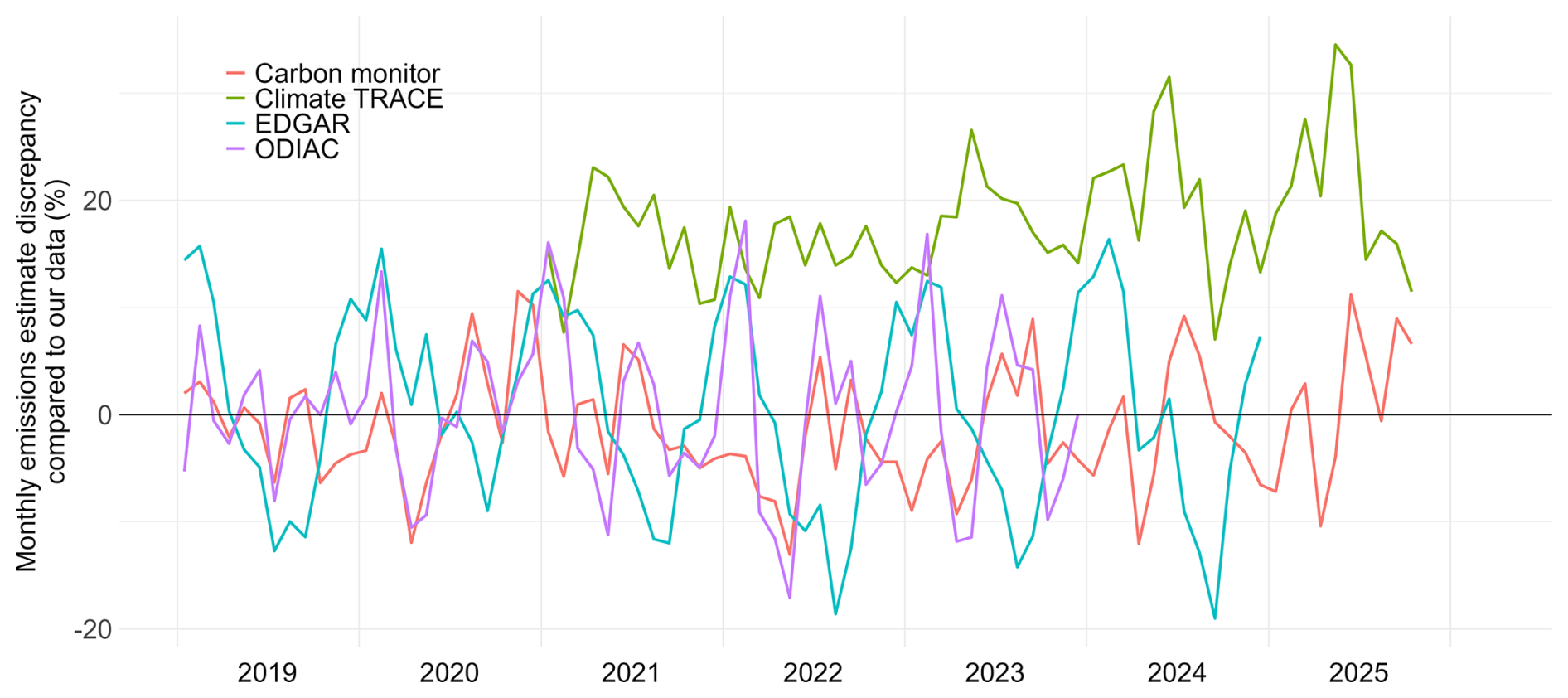
Figure 13Monthly differences in the estimates of four datasets compared to our monthly estimates.
3.6 Comparison of monthly estimates with other studies
In Sect. 1.3, we summarized other sub-annual estimates of Japan's fossil CO2 emissions in the literature that can be compared to our estimates. The level of dependency on official activity data or reported emissions varies widely across these datasets. In cases where the datasets are not anchored to official reporting, they may be vulnerable to additional biases, drift, and other deviations. In this section, we compare these monthly estimates quantitatively with our own estimates, and discuss how the discrepancies seen come from the construction methods.
Table 2Quantified differences between alternative datasets and our monthly estimates.
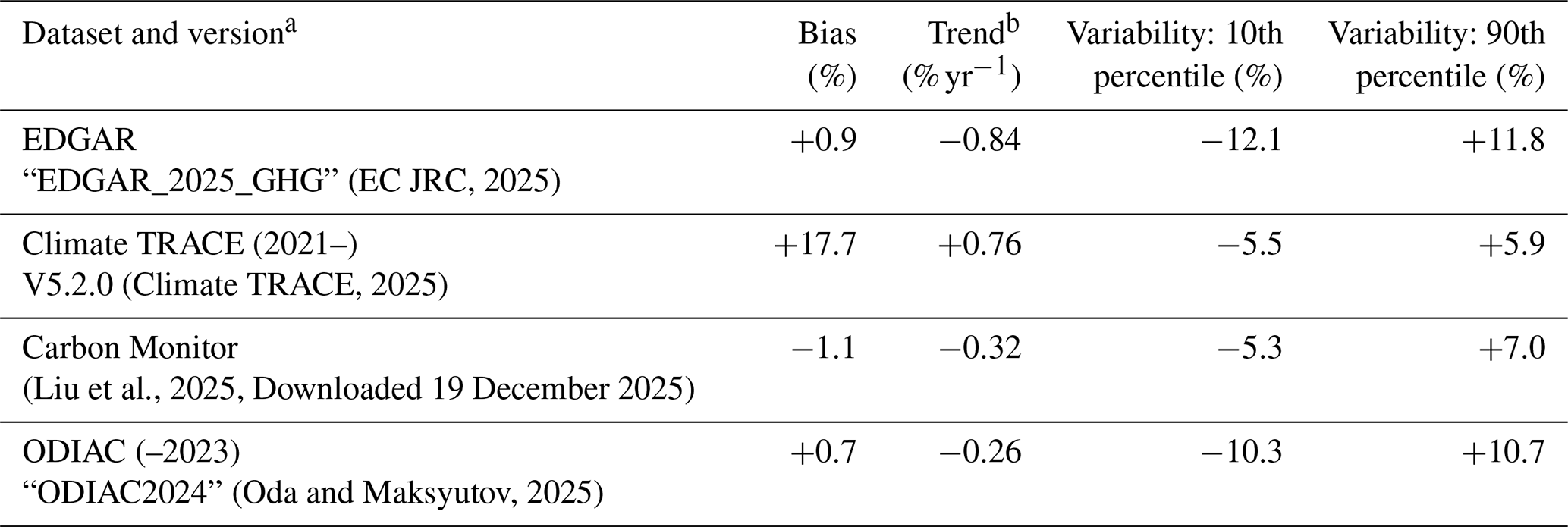
a 2019–2024 unless stated b none are statistically significant
Figure 12 shows monthly emissions estimate of our dataset for the period of comparison, while Fig. 13 shows the monthly relative differences of four alternative datasets compared to our estimates. See Appendix L for a figure showing absolute values of all datasets, not shown here due to high visual density. Table 2 shows the bias, trend and variability of the estimates, compared to our monthly estimates. The biases and trends are estimated using a simple linear regression in the relevant period. To quantify the size of the variability, we show the percentile values of the monthly discrepancy at 10 % and 90 %.
Below, we outline what each dataset exhibits and provide interpretations based on how each of the datasets is constructed. An important preface is that none of these other datasets focus solely on Japan, and are rather global in coverage, but they nevertheless present detailed emissions for Japan. All four datasets exhibit only small differences in trend compared to our dataset, all being within 1 % yr−1, although none of these differences are statistically significant. In the following discussion we refer to “monthly profiles” in the sense EDGAR uses, i.e., the share of each month's emissions in annual emissions; this abstracts away from the absolute level of emissions to just look at the monthly form.
3.6.1 EDGAR
EDGAR's annual emissions are constrained to be relatively close to national reporting by virtue of their derivation largely from IEA's energy data using the Reference Approach, and IEA's data are in the main provided directly by national agencies. Exceptions to this are mostly in the carbonate decomposition categories, which are significantly smaller than the energy categories. As with the NIR, the IEA data is based on fiscal year annual values for Japan (IEA, 2025), but the connection to officially reported energy data suggests a priori that EDGAR's monthly emissions would show both low bias and a low trend deviation compared to our results, which is what we observe in Fig. 13.
However, while the EDGAR dataset is available with monthly resolution, our analysis indicates that 21 of the 27 sectors exhibit no intra-annual variation in Japan in the last ten years: their monthly profile is exactly the same every year. Even in 2020, at the height of pandemic lockdowns, EDGAR's monthly data for Japan's road transport emissions show no deviation from the pattern of other years. While those six sectors with a varying monthly profile made up 35 % of total emissions in 2024, the inter-annual variation of the largest varying sector – Public electricity and heat production, making up 44 % in 2024 – was minimal (Fig. D1).
EDGAR's monthly profiles are intended in a sense to be the “normal” spread of annual emissions across months in each sector and country, and therefore by design cannot capture real-world variations from year to year.
In addition to the general lack of inter-annual variation in EDGAR's monthly profiles, some monthly profiles clearly reflect a lack of information. The monthly profile of the domestic aviation sector is set to be equal each month, indicating a lack of information about how June differs from May, for example. In fact, the share each month does not reflect the number of days in each month, leading (probably unintentionally) to higher daily emissions in February (28–29 d) than in January (31 d). Moreover, because of the precision used to represent EDGAR's monthly profiles, becomes 0.08333, and 12 × 0.08333 is less than 1.0 so the residual has been added to December, making that final month 0.08337, higher than all other months only to maintain balance.
With the lack of inter-annual variation in many sectors, it is unsurprising that EDGAR's monthly emissions estimates vary by almost 20 % in individual months (Fig. 13).
3.6.2 Climate TRACE
Japanese emissions reported by Climate TRACE v5.2 show a large bias and are considerably higher than our estimates and those officially reported by Japan, although with a low difference in trend. The methods used by Climate TRACE vary considerably between different sectors.
In the road transportation sector, for example, Climate TRACE has annual emissions in 2023 of 279.1 Mt CO2, while Japan's CRT indicates 163.0 Mt CO2. Climate TRACE's method first estimates traffic flow on individual road segments using spatial snapshots from a road-network database and satellite imagery and a model based on US training data. They then combine this with the share in the vehicle fleet (not absolute numbers) of different vehicle types and engine types, country-specific fuel efficiencies, and standard fuel-combustion emission factors to produce an estimate of emissions for each road segment. It is not explicitly stated whether they differentiate temperature effects in non-plugin hybrid cars, where the range of the electric motor varies considerably with ambient temperature (Steinstraeter et al., 2021), and this could be important in Japan with its very large fleet of such cars. Since the Fall 2024 update, Climate TRACE has introduced a global scale factor so that global emissions in the road transport sector match those of EDGAR in 2021–2022, recognizing bias in their training data (Kott et al., 2024). In the Fall 2025 version, this global scaling factor was about 0.8. Despite this large global downward scaling, the bias when compared to our estimates for Japan remains high.
With respect to seasonality in the road transport sector, however, the largest issue is probably that Climate TRACE's road transport emissions estimates are fundamentally annual, and simply interpolated to give daily data, then aggregated to months for dissemination. The only sub-annual factor in the model appears to be the temperature effect on fuel efficiency, which will not capture any changes in driving distances throughout the year. Since Climate TRACE's data start in 2021, we cannot observe the effect this would have had on their estimate of Japan's road transport emissions during the pandemic lockdowns in 2020.
Apart from the road transport sector, we note that Climate TRACE has recently begun to shift from using AI-derived activity data from satellite imagery for the power sector to use of actual, reported activity data (generation) where monthly facility-level data are available, but this is not the case for Japan (Freeman et al., 2025). This methodological change has led to very large changes in their power-sector estimates in the countries for which it has been introduced (e.g., India, Fig. E1), suggesting that the AI-satellite method might not always perform well.
Our analysis of Climate TRACE data shows that of the 35 power plants in Japan running only on natural gas in 2024, 33 had identical monthly emissions profiles (Fig. D2). Analysis of the detailed confidence statistics provided with Climate TRACE's data shows that estimates of emissions for all power plants in Japan over all months of the dataset were allocated very low or low confidence. In 96 % of cases, gas power plants were estimated using the “baseline” method and only 4 % with the method based on AI and satellites. The baseline method starts with annual generation and capacity data by fuel type sourced from EIA and EMBER, derives an average-annual capacity utilization factor, and applies that to all plants in the country for that year (Freeman et al., 2025). Monthly disaggregation is performed by combining the outputs of two models that provide sub-annual estimates of power demand for an average year, in one case based on temperature and GDP (Mattsson et al., 2021) and in the other on actual Japanese national demand data for the year 2015 (Brinkerink et al., 2021). Given the importance of the power sector in Japan's emissions, Climate TRACE's use of average sub-annual profiles appears to explain much of the differences we observe in seasonality compared to our results based on officially reported activity data.
3.6.3 Carbon Monitor
Carbon Monitor's bias when compared to our estimates is low, at an average −1.1 % across the overlapping period, and the trend difference is also low. The reason for this is that Carbon Monitor – for editions released in late 2025 and later – is anchored to Japan's official, annual emissions estimates for the years 2019–2022 (Liu et al., 2025). In practice this means that now the total emissions reported by Carbon Monitor in each of those years should match official annual reporting and the various proxies are used to temporally disaggregate. Beyond 2022, the growth rates of the chosen proxies will determine the bias and trend. Until this change in late 2025, Carbon Monitor was anchored only to EDGAR data in 2019, leading potentially to more drift from the anchor point over several years in previous editions since proxies don't capture all changes. An example is the use of traffic congestion as a proxy: this takes no account of changes in fuel efficiency of vehicles, particularly a transition to electric vehicles. Extended use of proxies many years from the anchor point could therefore lead to significant drift. Turning to seasonality, more than half of the sub-annual variability (max-min) in Carbon Monitor's data for Japan in 2024 is driven by the power sector and given that actual national generation data by fuel type are used as a proxy, we would expect this to be relatively well captured, as long as the time-invariant emission factors used are good approximations. If, however, the true emission factors vary between power plants of the same fuel type (coal, natural gas, petroleum), then the shifting balance of how much each power station generates will shift the true average emission factors higher and lower than the time-invariant values used by Carbon Monitor.
For the industry sector, Carbon Monitor uses a single industrial production index, which may not reflect real temporal changes in emissions across all industry. As a toy example, we could imagine an economy that has two industrial sectors of about the same size, where only one of these two sectors emits CO2, and the two sectors have opposite seasonality: during the 6 months that one is producing, the other is not producing, and vice versa. In this situation, the industrial production index might be constant throughout the year, but the emissions most certainly would not be. Without having real sub-annual data by different industries in Japan, it is impossible to know how wrong the use of a single industrial production index would be in estimating monthly industrial emissions, but certainly the possibility exists.
In the case of the ground transport sector, which contributes about one-sixth of Japan's carbon emissions, Carbon Monitor has since its introduction in 2020 used a regression model based on emissions in Paris as a function of a traffic congestion index and applied this model to all countries. In Japan, this traffic congestion data was available only for five urban areas (Liu et al., 2025). It is far from clear that this out-of-sample application is appropriate, and Oda et al. (2021) demonstrated that these estimates varied significantly from estimates derived directly from official fuel consumption data. While the proxy method at least gave the appearance of avoiding the tertiary stocks problem, the method used by Carbon Monitor changed with the November 2025 release (Fig. F1), and now the use of the traffic-congestion proxy has been replaced with use of reported fuel data, where available (Zhu Deng, personal communication, October 2025). The estimates published in November 2025 for Japan used reported monthly domestic sales of gasoline to generate seasonality (Fig. F2), although the method appears to have changed again since then.
Despite the apparent use of officially reported sub-annual statistics for two of the most important emitting sectors (power and road transport), Carbon Monitor's monthly estimates still differ by as much as 10 % in individual months from our estimates, which are almost entirely based on official statistics. The fact that our estimates are disaggregated by fuel types while Carbon Monitor's are disaggregated by sector hinders further comparison.
3.6.4 ODIAC
The ODIAC dataset exhibits both low bias and low trend compared with our estimates. Again, ODIAC is indirectly connected to officially reported data since it starts with annual national emissions from CDIAC-FF, which in turn are derived from UN energy data, which are to a large extent officially reported by countries. This anchoring of annual emissions in official reporting would a priori be expected to cause a low bias and trend compared to our estimates, which are derived directly from official reporting.
For seasonality, ODIAC's data have a similar deviation to EDGAR's from our dataset, with variability at both the 10th and 90th percentiles above 10 %. However, ODIAC has two distinct methods for temporal disaggregation, with use of monthly profiles from Andres et al. (2011) up to and including 2019, and a change to the use of Carbon Monitor from 2020 (Maksyutov and Oda, 2025). While the version of Carbon Monitor used by ODIAC 2024 was prior to the major changes to methods by Carbon Monitor towards the end of 2025 – explaining the differences in Fig. 13 between the seasonalities of ODIAC and Carbon Monitor – we limit our discussion here to the period up to 2019 and the use of Andres et al. (2011).
For the period 2000–2019, ODIAC's seasonality is derived from an average seasonality for the period reported by Andres et al. (2011). Oda et al. (2018) call this average the “climatological seasonality”, and recognize that use of a non-varying sub-annual seasonality “could be a source of uncertainty and bias” (Oda et al., 2018). Effectively they attempt only to capture the normal variations because of an assumed constant climate, without any attempt to capture any other variations caused by weather, markets, geopolitical events, demand shifts, technology changes, or other socioeconomic factors. Andres et al. (2011) obtained monthly fossil fuel (coal, oil, gas) sales data for the years 1977–2002, which by 2019 were already relatively old, such that the true monthly profile in 2019 will probably have drifted somewhat from the monthly profiles derived from those early data.
We note also that ODIAC is a gridded dataset that inseparably includes international bunker fuels, so in masking out Japan's territory from the grid, the “ODIAC Japan” that we are comparing to does not have quite the same system boundary as our territorial emissions estimates, which exclude all bunker fuels.
The monthly emissions data for all emission categories described in Sect. 3.1, together with the input trade and activity data to produce these, are available on Zenodo at https://doi.org/10.5281/zenodo.20023226 (Kunimitsu and Andrew, 2026), and updated versions will be released periodically as additional data become available.
We have created a novel monthly dataset of fossil fuel and industrial process carbon dioxide emissions in Japan. Our dataset is derived almost entirely from officially reported sub-annual data and official energy contents and emission factors, and comparisons with Japan's official, annual reporting to the UNFCCC show very good agreement. Our analysis of key areas of uncertainty shows that while there are many factors that may lead to uncertainties, stocks are potentially the largest factor with difficulty in quantification. Beyond stocks, the dominant uncertainty comes from those in coal activity data that are also present in the annual official estimates, and these dominate the uncertainties at the monthly level as well. We obtained monthly emissions uncertainty of around 3 %, which is remarkably low by international standards especially when thinking of monthly emissions, but not implausible given that a large portion of emissions come from the energy sector where monthly statistics are recorded with high accuracy and with the same IPCC-aligned methods as the annual data, and also given that the trends in demand and production in Japan are relatively predictable. The uncertainty is well within the monthly variations, and means that our estimates can be used with high confidence to assess implications from monthly emission changes.
Comparison of our estimates with other available monthly datasets showed in three of four cases no significant bias in the average emissions across time, with Climate TRACE being the exception with larger bias. The core difference is in how much each dataset is anchored to officially reported data, with our estimates being almost entirely anchored to both monthly and annual official data. EDGAR and ODIAC are both largely constrained at the annual level by nationally reported energy data via the IEA and CDIAC-FF/UN, respectively. Carbon Monitor relies on nationally reported electricity generation and in the most recent editions also on both nationally reported road-fuel data and total emissions from reporting to the UNFCCC. The recent updates to Carbon Monitor's method have reduced potential for drift as proxies are used to extrapolate out from the anchor points.
However, the seasonality component exhibits large variation between datasets, much of which can be attributed to the methods by which monthly profiles are developed. In the cases of EDGAR and ODIAC, monthly profiles are mostly fixed and therefore represent an average sub-annual pattern, which cannot capture the many changes from year to year in sub-annual patterns. ODIAC has more recently shifted to using Carbon Monitor directly for sub-annual disaggregation, but only from the data year 2020, with earlier years still using fixed profiles. Climate TRACE has begun to move away from using fixed monthly profiles in the power sector, but apparently not yet for Japan due to a lack of the data required by their new method. It is clear, therefore, that some of these datasets with sub-annual temporal resolution are moving further along the spectrum from relying almost entirely on proxies to relying almost entirely on officially reported data as in this study. While this shift ought to lead to improved estimates, using valid proxies has three advantages: (i) proxies are potentially available earlier than official activity data, (ii) they may be available for countries that do not officially report sufficient sub-annual activity data, and (iii) they can potentially capture the timing of consumption, for example, and ameliorate the tertiary stock issue. The tertiary stock issue is potentially important for inversion modelling, but further quantification of its effect is required. Since not all countries officially report the sorts of data required for directly estimating emissions, proxy-based methods remain important for estimating sub-annual emissions in many – particularly developing – countries.
Methods based on limited anchoring and proxy extrapolation have proved and will continue to prove useful for estimating sub-annual emissions globally, and while the approach we have presented for robust estimates for Japan could also be taken for other countries, the methods and data sources are highly specific to Japan and cannot be replicated directly to other countries. However, our investigation of some of the temporal disaggregation methods used by other datasets demonstrates that the quality of proxies chosen varies considerably across datasets and across sectors, and that proxy-based methods should be treated as having relatively high uncertainty.
With the development of the monthly emissions data, we now have a near-real time update of accessible emissions data, as well as detailed sub-annual trend data of historical emissions. This potentially has many applications, and while we defer to future studies of specific analyses of historical data, we focus on three key potential uses here: policymaking, public awareness, and independent verification.
Having data only at annual resolution and with a 12-month publishing delay significantly reduces understanding of the reasons behind emissions changes, which in turn can lead to more poorly targeted policy and therefore less effective mitigation. This long lag creates distance between policymakers and the results of their policies, thereby reducing political responsibility for failure or success, and it delays any necessary course corrections to climate policies that are less effective than expected, to non-climate policies that are having undesirable effects on emissions, or to the absence of policies. Our estimates of Japan's emissions have low uncertainty, monthly temporal resolution, and a low lag of only 2 months, effectively providing significant new information for the use of policymakers to address these issues.
More frequent updates to emissions estimates provide more opportunities to discuss emissions, responsibility, and climate action in Japan. Media discussion of climate change in Japan has mostly focused on international events such as the annual UNFCCC Conferences of the Parties (COPs) (Ida and Emori, 2025). Just as frequent releases of economic data keep the subject alive in the public consciousness, so might more frequent releases of emissions and other environmental data do so, helping to increase accountability, public pressure for action, and awareness of Japan's role in global environmental change.
Emissions estimates with high temporal resolution are important for the developing field of atmospheric inversion modelling, which aims to verify reported emissions. Such models use satellite observations of atmospheric greenhouse gas concentrations to estimate where the gases were emitted (Chevallier et al., 2005). However, such models are still very poorly constrained by independent observations and rely heavily on bottom-up estimates of emissions. For Japan, we argue that our monthly estimates are considerably more accurate than other bottom-up estimates that have been used in the inversion-modelling community. However, further disaggregation – both temporal and spatial – is still required.
Our robust and easily updated estimates lay the ground for more sophisticated analysis of trends in Japan's emissions, including effects of weather, policy and geopolitical factors. Because our method is based on actual reported data, rather than simplified models, it will capture all out-of-sample events such as the pandemic lockdowns, economic crises, and changes in technology. Moreover, our monthly estimates could be further disaggregated to daily or higher temporal resolution using the same simple methods used in other datasets (such as Carbon Monitor) and also disaggregated spatially using additional information.
A detailed analysis of possible policy implications based on the monthly emissions data is a topic of further study, but the very compilation of such monthly emissions data can also have impacts on policy, for example through the raised awareness of emissions level and change when publicizing the updated data. While measurement and monitoring alone are insufficient to initiate action, their absence certainly hinders effective action, and there is significant scope for estimates such as ours to form the basis for action towards lower emissions in Japan.
Here we describe the details of the data listed in Table 1.
A1 Primary Fuels
We first describe data on primary fuels, which are fuels found in nature (crude oil, coal, natural gas).
A1.1 Crude oil, Natural gas liquids (NGL), and Bituminous mixture fuel
METI publishes a monthly report on petroleum statistics (METI, 2026e), which is based on a census (i.e. 100 % coverage) of all companies handling crude oil. This includes the consumption of crude oil, as well as production, import, and inventory. The data are available in machine-readable form from 2007, but only available in scanned PDF format for 1989–2006. We read the data from the PDFs using optical character recognition (OCR).
“Consumption” of crude oil as used in this dataset does not match the categories used in the NIR; “consumption” here includes crude oil used for refining and also natural gas liquids (NGL), while unrefined crude oil used for example for electricity generation is excluded. This is not explicitly mentioned but is safely inferred from comparison with annual data. There are separate monthly data for use of unrefined crude oil which can be added in. There are no data published at monthly frequency that separate NGL from crude oil. Monthly values for NGL can be reconstructed from the Yearbook of Mineral Resources and Petroleum Products Statistics, which has much more detailed data compared to the monthly report, but this is published annually, so these monthly values can only be reconstructed with annual lag. While we cannot determine the amount of crude oil consumption separately from NGL, our purpose is to estimate the total emissions, so we present the sum of crude oil and NGL.
In addition to these, the category of primary liquid fossil fuels in the NIR includes “Bituminous mixture fuel” (reported as “Orimulsion” in the CRT, although not necessarily the true product Orimulsion), obtained by mixing with water. This is used in Japan solely for electricity generation purposes, and the monthly data on consumption can be obtained through the Electricity Survey Statistics (METI, 2026c), but the Japanese government has recently reclassified much of what was reported here as other oil products after inspection of their actual origins (METI, 2023). While there is some usage reported after the revision, these are still minor, so we decide to exclude these in this study.
A1.2 International bunker fuel
The IPCC guidelines require that NIRs exclude sales of international bunker fuels – fuels sold to vessels undergoing international transport, i.e. international aviation and maritime transport – from estimates of national total emissions, but that they are to be reported as a memo item in the CRT (specifically, Table 1.D). Given that our goal is to produce monthly estimates of Japan's territorial fossil CO2 emissions aligned with its official reporting, we make no effort to quantify bunker fuels in our dataset. Importantly, domestic monthly consumption data in Japan already exclude this amount and only include the domestically consumed amount.
A1.3 Coal
While the Japanese government publishes partial statistics on the use of coal in electricity generation (METI, 2026c), it does not publish monthly statistics on total coal consumption, and publication of monthly domestic production data was discontinued at the end of 2001. However, given that annual domestic production has been below 1 % of total consumption since 2002, use of import data published by the Ministry of Finance (MOF, 2026) will be a good estimate of total supply. Data from 1998 to 2008 are in PDF format, which has been extracted to machine-readable form (Andrew, 2025). We also extracted trade data prior to 1998 from the MOF database with manual prompts. For domestic production from 2002, we disaggregate the annual domestic production statistics into months using a linear disaggregation method (see Appendix B).
Import categories provided by the Ministry of Finance are subdivided into three categories: Anthracite, Coal of coking (sic), Coal not elsewhere specified. At first glance, these appear to match the categorization used in the CRT: Anthracite, Coking coal, Other bituminous coal (and Sub-bituminous coal, which refers to domestically produced coal). But one subcategory within “Coal of coking” from the trade data (“BITUMINOUS COAL, ASH CONT. WT = < 8 %, N.E.S.”) is included in “Other bituminous coal” in the CRT. This matters for emissions estimation since the conversion factors used are different between categories.
We take conversion factors from METI's annual reporting. For coal, METI does not publish data for measured conversion factors, so the values used here are identical to the domestic standard factors (Sect. 2.3).
The METI categorization of coal corresponds to the CRT categories: Steel Making Coal, Steam Coal, “Hard Coal, Anthracite & Lignite”. Steam Coal corresponds to “Other bituminous coal” and “Sub-bituminous coal” in the CRT. But for Steel Making Coal, the factor used is the weighted average of two subcategories (Coking Coal and Pulverized Coal Injection Coal) which does not correspond to trade data, and for Steam Coal, separate factors need to be used for “Imported Steam Coal for Power Generation Use”, which again does not have corresponding trade data. The CRT factors are adjusted for these, so there is no difficulty in comparing with existing annual data, but these details will become important when extrapolating beyond the period covered by the NIR.
A1.4 Natural gas
The Japanese government does not publish monthly statistics on natural gas consumption, although partial statistics regarding electricity generation (METI, 2026c) and a survey of large suppliers (METI, 2026b) are published. We therefore rely on the use of import statistics from the Ministry of Finance (MOF, 2026). As with coal trade data, we use early data extracted from PDF format (Andrew, 2025) and from the MOF database. All import of natural gas to Japan is in the form of liquefied natural gas (LNG), since Japan has no pipelines from foreign nations. All LNG is imported.
In addition, monthly production data for natural gas is published by the Japanese government (METI, 2026d). Domestic production comprises around 2 %–3 % of the total gas consumption in energy terms for the past 10 years. Given gaseous fuels have different measurements depending on the state of the gas (i.e. pressure and temperature), a conversion factor needs to be applied to match the units used for the GCV factors used by the Japanese government. There is no direct reference for this conversion factor, but applying ideal gas equations replicates the officially used values (see Appendix H).
A2 Secondary fuels
A large portion of primary fuels, especially crude oil, is transformed into secondary fuels. While fuel use of these products produced from primary fuels is already accounted for in the reference approach values of primary fuels, there is also direct import and export of these secondary fuels that change the net amount, as well as non-fuel use that does not lead to direct CO2 emissions. Thus, we need to incorporate data for secondary products regarding trade and non-fuel use.
Following the IPCC guideline categories (Eggleston et al. 2006) for secondary fuels, we include for liquid fuels the following: Gasoline, Jet kerosene, Other kerosene, Gas/diesel oil, Residual fuel oil, Liquefied petroleum gases (LPG), Naphtha, Bitumen, Lubricants, and Petroleum coke. For solid fuels, we include Coke oven/gas coke and Coal tar.
For fuel trade, we use data from either the monthly report on petroleum statistics (liquid fuels except petroleum coke) or the Ministry of Finance trade data (for solid fuels and petroleum coke). For non-energy usage, we take values from the Current Survey of Energy Consumption2 (METI, 2026a), in line with the annual values published in the General Energy Statistics. The exceptions are described in the following sub-sections.
A2.1 Naphtha
Naphtha has the largest apparent consumption among secondary fuels, yet it also has the largest non-energy usage value mainly because of its use in the chemical industry, resulting in a relatively minor net contribution to overall emissions. The monthly statistics of non-energy usage reported in the Monthly Report of the Current Survey of Energy Consumption (METI, 2026a) include fuel byproducts generated in the production process of ethylene and BTX (benzene, toluene, xylene). This is excluded in the NIR reporting, so adjustments are made by combining the production statistics of Ethylene and BTX from the Monthly Report of Current Production (METI, 2026d). Details of this are described in Appendix C.
A2.2 Lubricants and Bitumen (Asphalt)
For these secondary fuels, the monthly consumption statistics do not provide non-energy usage data. In both cases, monthly data are likely not available elsewhere; the Japanese government estimates annual values for lubricants consumption – largely for transport – by scaling FY 2000 consumption by total driving distance, while they estimate asphalt consumption from annual forecasts on use, neither of which allow monthly measures. Thus, we disaggregate the reported annual value to monthly values by a linear fit described in Appendix B.
A3 Industrial processes
A3.1 Cement production
The production of cement releases CO2 when producing clinkers from limestone (Eggleston et al., 2006). Monthly clinker production data are available through the Monthly Report of Current Production Statistics (METI, 2026d), which is based on surveys of producers above certain thresholds in size. Data for 1989–2006 are published in scanned PDF format, thus we combined optical character recognition (OCR) and manual transcription to process these.
We apply the emission factors reported in the NIR to estimate monthly emissions from the monthly data. The value ranges from 0.505 to 0.516 (CO2 weight per clinker weight), varying according to the amount of CaO and MgO within the produced clinker coming from limestone. Almost all cement kiln dust (CKD) is recovered in the production process, so there is no correction associated with this. Following the reporting guidelines, emissions from input energy used in producing cement are included in the Energy sector.
A3.2 Lime production
As with cement production, the production of lime leads to CO2 emissions when processing limestone. Monthly lime production data are available through the Monthly Report of Current Production Statistics (METI, 2026d). These data include values for both quick lime and slaked lime, but slaked lime is produced from quick lime already reported within the statistics (METI, personal communication), so to avoid double counting, we derive emission from the data on production of quick lime only. As with cement, we include data extracted using OCR for the period 1989–2006.
The emissions reported in the NIR, on the other hand, are based on the amount of limestone consumed for lime production. This part of the estimation method is in line with the IPCC Tier 3 method, although the NIR does not claim to use the Tier 3 method for lime. The NID refers to the Adjusted Price Transaction Table for the limestone consumption data, but the table is not available to the public. Thus, production amount cannot be directly compared with the annual reference value, and we only compare the emissions amount between the two data series.
As with cement production, the emissions factors are taken from the NIR reported value, which in turn comes from the Japan Lime Association. The value is 0.748 (CO2 weight per lime weight produced3), constant throughout the reported period.
A3.3 Pig iron production
While coal used to produce pig iron is accounted for in the coal consumption statistics, the production process also includes the heating of limestone and dolomite to remove impurities from the molten metal, and this leads to the release of CO2. The amount of CO2 released is comparable to the amount from lime production.
The monthly production value of pig iron is available in the Monthly Report of Current Production Statistics, but the values reported in the CRT are in terms of the limestone consumed, which has no corresponding monthly statistics available to the public. We disaggregate the annual emission values proportionally to the monthly production of pig iron, assuming limestone usage is also proportional. This is plausible for single years, and while there is some variation trend throughout the years (Sect. 3.1), the emission to pig iron production ratio has stayed mostly within the range of 0.07–0.08. We use the most recent value to extrapolate to the latest year.
A4 Waste incineration
The NIR divides emissions from waste incineration into those coming from incineration accompanied by energy recovery (for example electricity generation or heat use), and those that do not. Monthly data for neither of these are available, so we make a linear disaggregation (see Appendix B) based on available annual data from the NIR for each category, and extrapolate to the latest year using values from the previous year.
Where monthly data is unavailable and only annual data exist, we disaggregate the annual value into months by weighting over 2 consecutive years, and then scaling by year so that the total of the months matches the total reported annual value. More specifically,
- a.
For each month of the year, we first set the emissions estimates by the following weighting:
Where En is the emissions amount in the nth month of the fiscal year FY, and EFY is the annual total reported in the NIR. For Japan, annual data are based on fiscal year (April–March), so we adjust the specific weighting for each month taking this into account.
- b.
For each fiscal year, scale each month with the same factor so that the sum of the emissions match the input annual year emissions:
With this method, we can account for long-term trends in the monthly data compared to a uniform disaggregation within year. We also avoid large steps in emissions between the last month of the fiscal year and the following month. This method has not been adjusted for days per month.
Non-energy usage of naphtha is defined differently between the METI General Energy Statistics, which is the annual statistics that the NIR activity data is based on, and the Current Survey of Energy Consumption, from which most of the monthly non-energy usage data of secondary fuel products come from. In the latter, all usage for the production of chemical products, namely the production of ethylene and BTX (benzene, toluene, xylene, including ortho-xylene and para-xylene), are included in non-energy usage, whereas in the former, the byproducts that are reused for energy are deducted. This difference comes from the different aims of the statistics, where the former is focused on energy balance, whereas the latter is focused on individual products.
In both datasets, naphtha is divided into (pure) naphtha and reformates, and the sum of these correspond to naphtha in the NIR. Around 40 % of the pure naphtha non-energy usage as defined in the consumption statistics consists of input into the production of ethylene, which results in byproducts that become energy sources, such as cracked gasoline. To account for this in the General Energy Statistics, the (pure) naphtha category subtracts the total amount of input to the production of ethylene from non-energy usage, while for the reformates category, the production of BTX is identified with non-energy usage. While monthly production of ethylene and BTX are directly accessible in the production statistics (METI, 2026d), the input from naphtha is not directly available, so we scale these monthly production values to match annual naphtha usage values for each available in the General Energy Statistics, and extrapolated the scaling factors to the most recent years (2024 and 2025). We estimate the monthly value of total non-energy usage starting from the non-energy usage value in the Current Survey of Energy Consumption, subtracting the scaled ethylene usage and adding in the scaled BTX usage. Ortho-xylene production values have become confidential since 2024, so are not included after that year. The annual total for years prior to 2023 matches the annual value reported in the NIR, by definition.
EDGAR's monthly emissions dataset is derived by applying “temporal profiles” to the annual emissions dataset. These temporal profiles are described by Crippa et al. (2020). The method is a framework that allows a different monthly profile for every sector-country-year combination, but in many cases variation does not exist along all three axes. Figure C1 shows the six sectors for which there is any variation between years in the monthly emission profiles in EDGAR's data for Japan. All other sectors exhibit no variation in the monthly emission profiles from one year to the next in the period 2015–2024. Of the six that vary, three have negligible variation across years (1A1bc, 2C, and 2G), while the largest emitting sector 1A1a shows only minor variation across years.
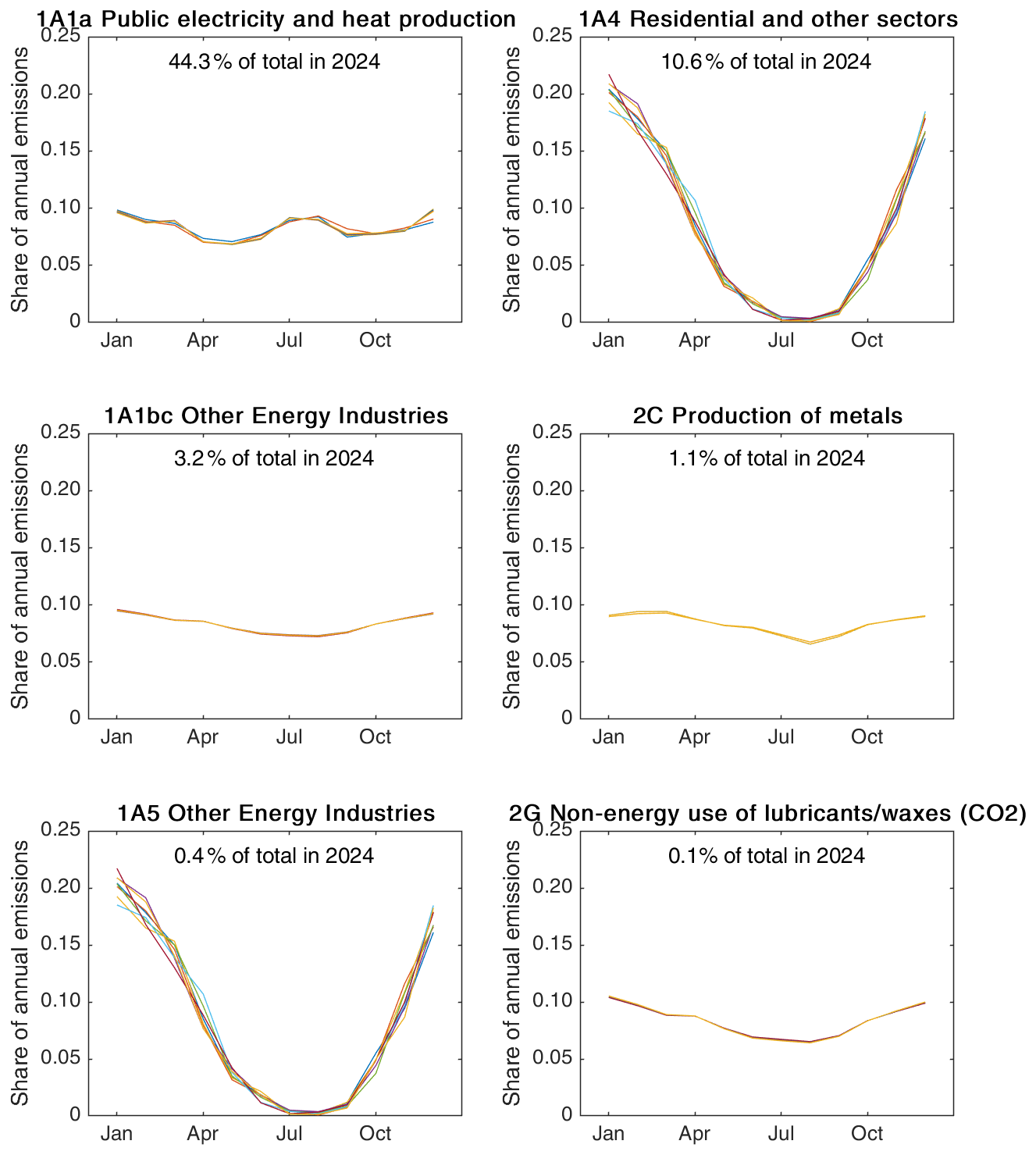
Figure D1Variation in the temporal profiles (monthly shares of annual emissions) in the six sectors that exhibit any variation out of the total 27 sectors provided by EDGAR. The different colors show the temporal profiles for different years, 2015–2024.
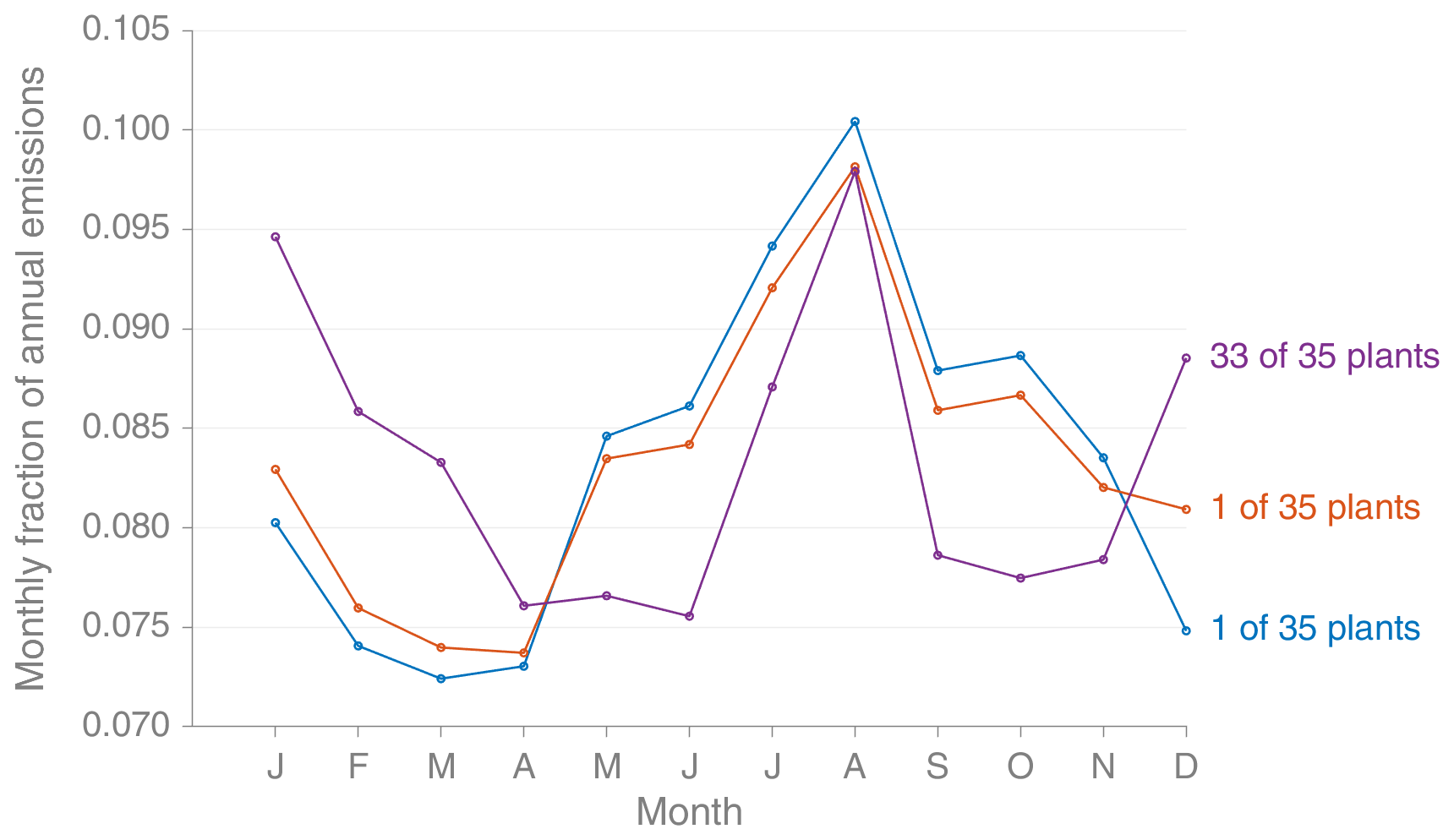
Figure D2The three unique monthly profiles in Climate TRACE's estimates of Japan's 35 gas-fired power plants (only those with “gas” as the fuel) in 2024, showing that for 33 of them the monthly profiles are identical: the monthly emissions in each of these 33 power stations have exactly the same temporal disaggregation from the annual estimate.
Figure E1 demonstrates the changes in Climate TRACE's methodology introduced in late 2025 for the power sector in the case of a large coal-fired power station in India. Before the change, activity data (plant-level generation) were estimated using a method based on AI detection of vapour plumes in satellite imagery. The figure shows that these estimates both lay significantly lower than actual, reported generation, and had a very different sub-annual pattern.
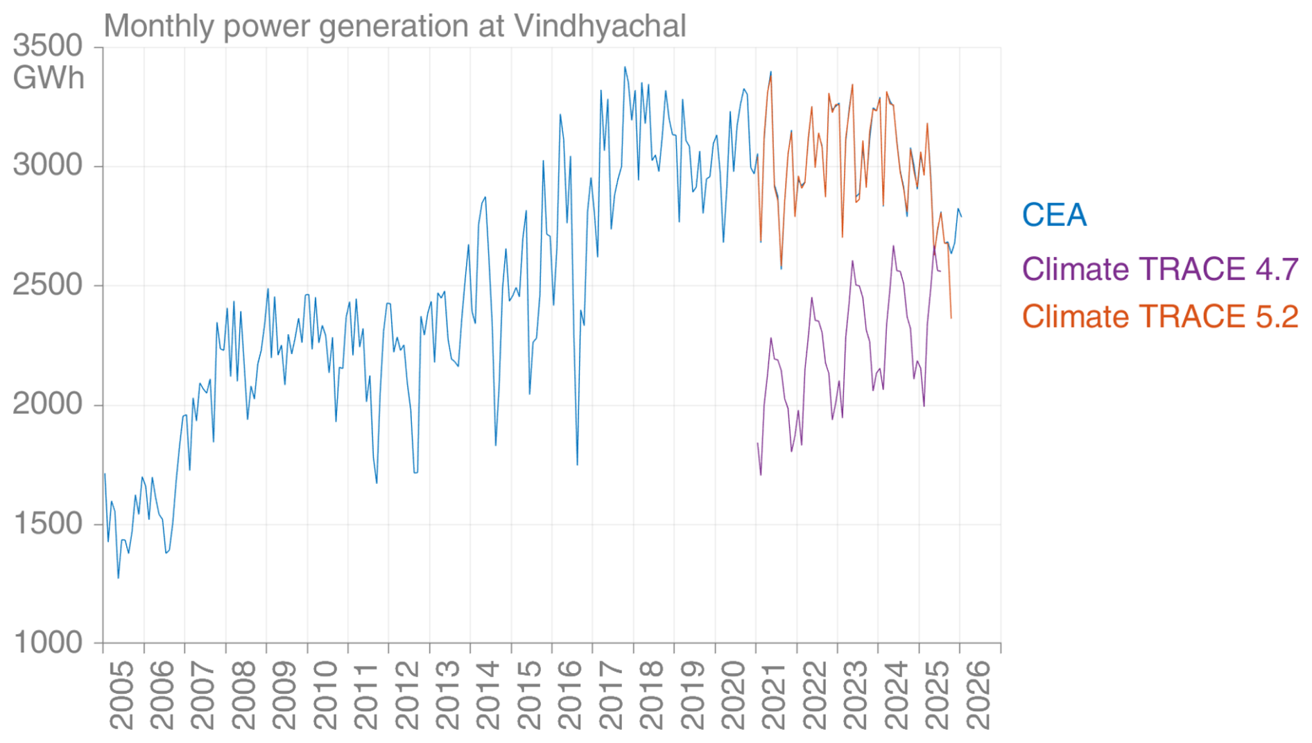
Figure E1Comparison of monthly generation from the Vindhyachal 4.8 GW plant in India, with reported data from India's Central Electricity Authority, the “baseline” estimates from Climate TRACE version 4.7, and the newer values from Climate TRACE version 5.2 after a methodological change. Apart from the final month, which is extrapolated, Climate TRACE's activity data are now directly from official reporting.
Carbon Monitor's estimates of road transport emissions in Japan changed significantly between the October 2025 edition and the November 2025 edition, indicating a change in method.
Noting that the intra-annual variation in gasoline supply reported by METI was identical to that of Carbon Monitor in its November 2025 edition, and applying a scale factor that only varies annually results in an exact match. The scale factor is about 1.65–1.70 in each year, and constant from 2022. Later editions of Carbon Monitor have changed again.
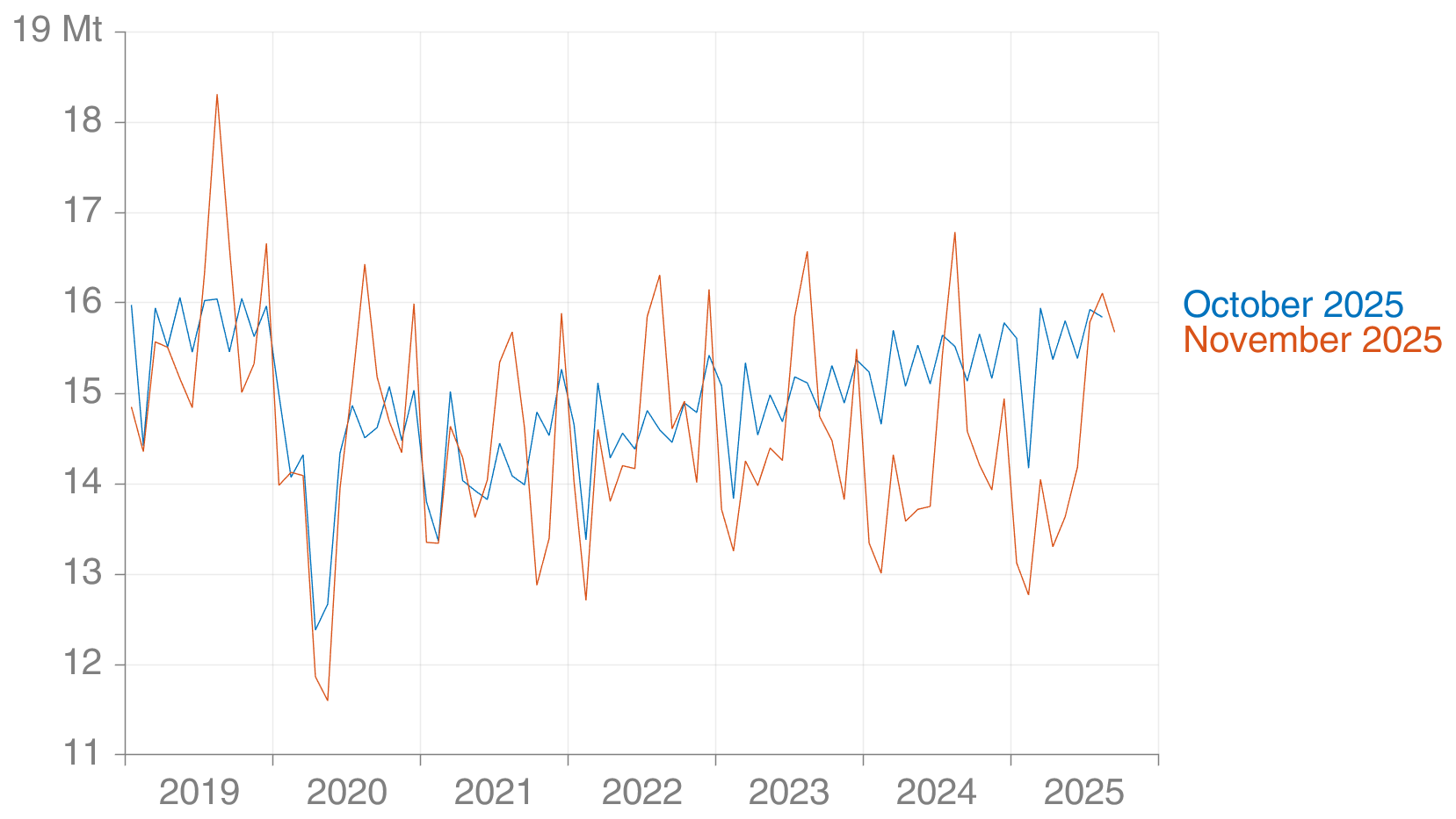
Figure F1Comparison of Carbon Monitor's estimates at monthly level for Japan's ground transportation sector.
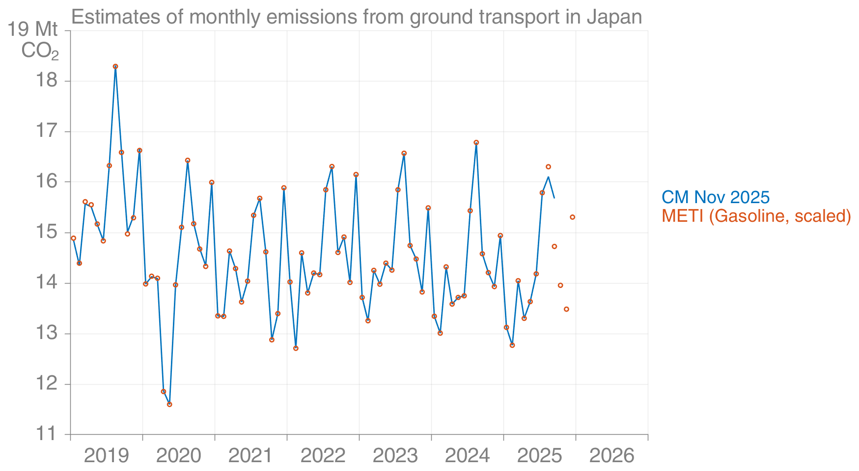
Figure F2Carbon Monitor's ground transport emissions in Japan (November 2025 edition) compared with gasoline supply data from METI, where the gasoline data have been scaled with an annually varying constant.
To illustrate the difference in the two accounting systems of territorial emissions and economic activity-based emissions, we show data for Ireland. While the UNFCCC NIR submissions are based on territorial emissions, the Eurostat quarterly estimates are based on the economic boundary to be aligned with national accounting (e.g., GDP) statistics.
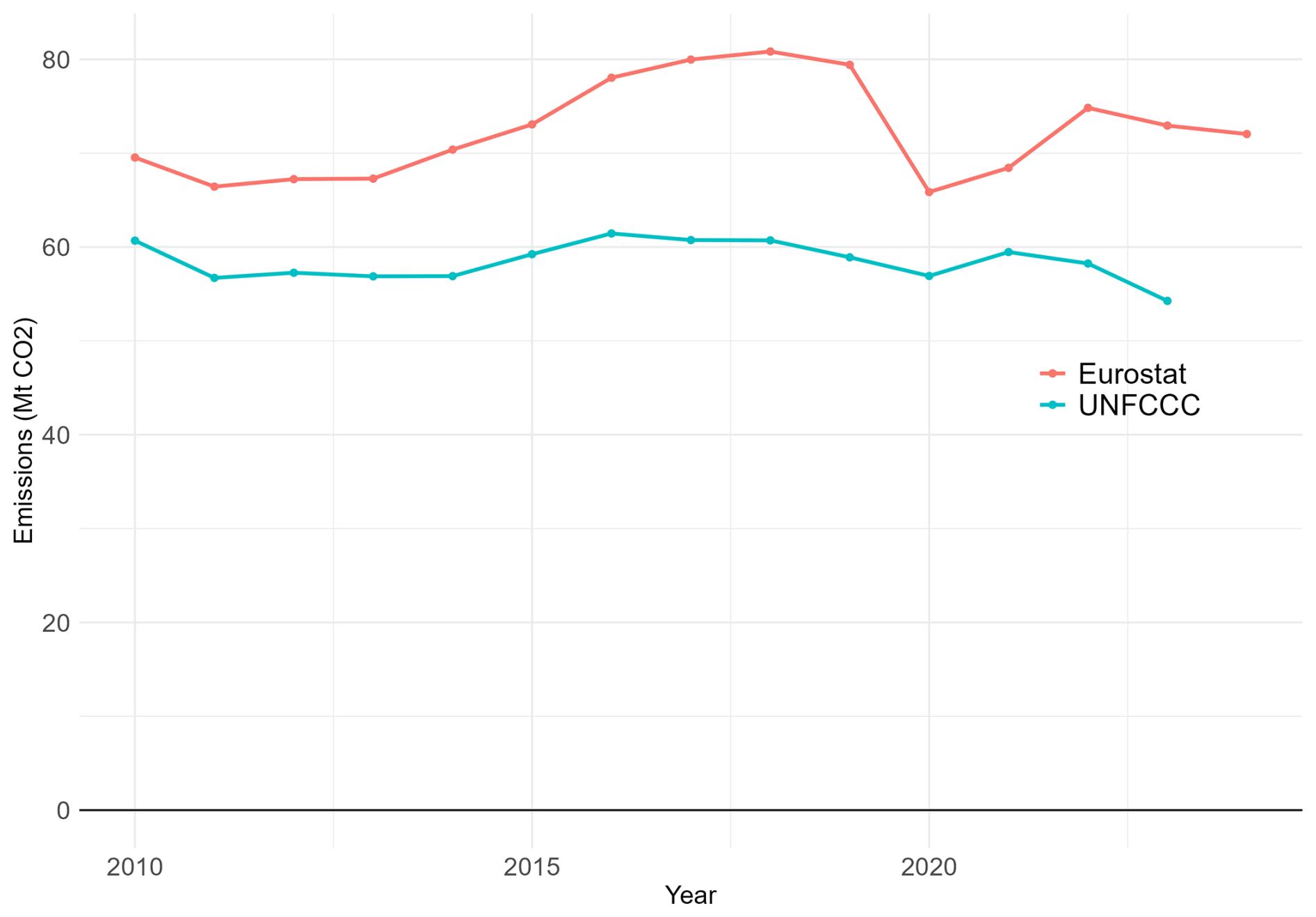
Figure G1Comparison of territorial emissions and economic activity-based emissions for Ireland, where the difference is particularly large.
As a gaseous energy source, the GCV for natural gas depends on the exact state the gas is in, but documentation on what conversion factor to apply is to be applied to the monthly data was not found. After examination, we identified the following information and conversion for monthly data to apply the METI GCV factor for natural gas: Monthly Report of Current Production Statistics uses 15.6 °C, 101.325 kPa, saturated with vapor; METI publishes a conversion factor to the above from the “normal condition”, which is 0 °C, 100 kPa, no vapor; GCV factor from METI is given for Standard Ambient Temperature and Pressure (SATP), which is 25 °C, 101.325 kPa, no vapor. We scale volume based on ideal gas equations, which result in a conversion factor of 1.027965 (volume to apply GCV/volume in monthly production report).
As discussed in the manuscript, Japan has been reporting detailed estimates of emissions to the UNFCCC for over two decades. By collating these reports, we can see that Japan's revisions to CO2 emissions have resulted in only very minor changes, and these have been negligible since the mid-2010s.
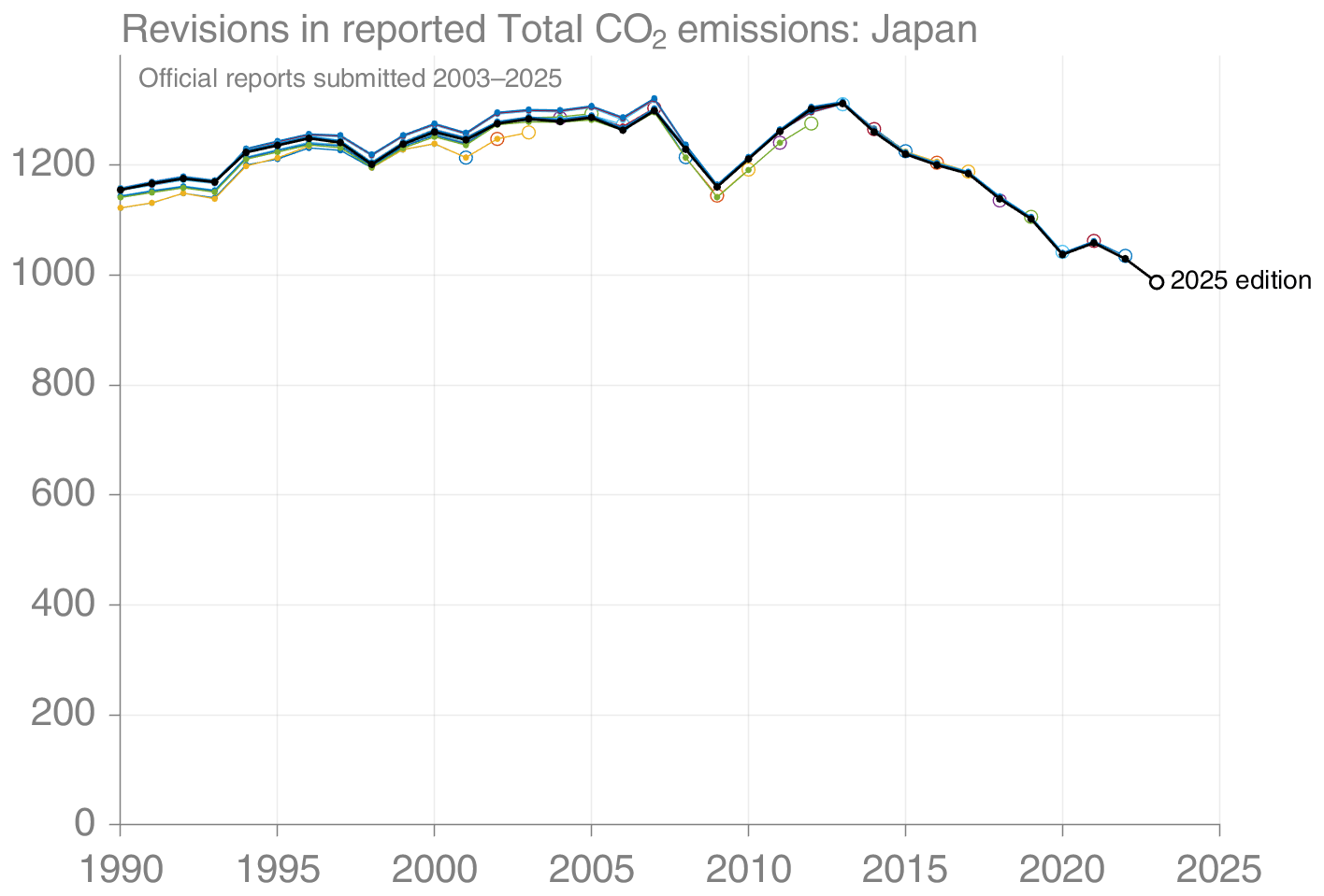
Figure I1Comparison of Japan's officially reported CO2 emissions. Most of the series plotted overlap. The final year of each series is indicated with the circle marker, and the final year is always two years before the edition number.
The following is a brief summary of the X-11 method, taken directly from Eurostat (2013, p.215):
- a.
Derive an initial estimate of the trend-cycle by applying a moving average to the raw data
- b.
Subtract this estimate from the raw data to obtain an initial estimate of the seasonal-irregular (SI) and apply a moving average to the SIs for each type of period (month) separately to obtain initial estimates of the seasonal component
- c.
Subtract the initial seasonal factors from the raw data to obtain an initial estimate of the seasonally adjusted series (i.e. the trend-cycle/irregular) and apply a Henderson moving average to obtain a second estimate of the trend-cycle
- d.
Subtract the second estimate of the trend-cycle from the raw data to obtain a second estimate of the SIs, and apply a moving average for each type of quarter separately to obtain final estimates of the seasonal component
- e.
Subtract the seasonal factors from the raw data to obtain a final estimate of the seasonally adjusted series and apply a Henderson moving average to obtain a final estimate of the trend-cycle
For Japan, the sectoral approach emissions estimate and the reference approach emissions estimate match very well, but this is not always the case for other countries. As an example of large discrepancy, we show the comparison of the two estimates for Norway. The large discrepancy, especially for liquid fossil fuels, is due to the large export and resulting statistical discrepancy in domestic consumption.
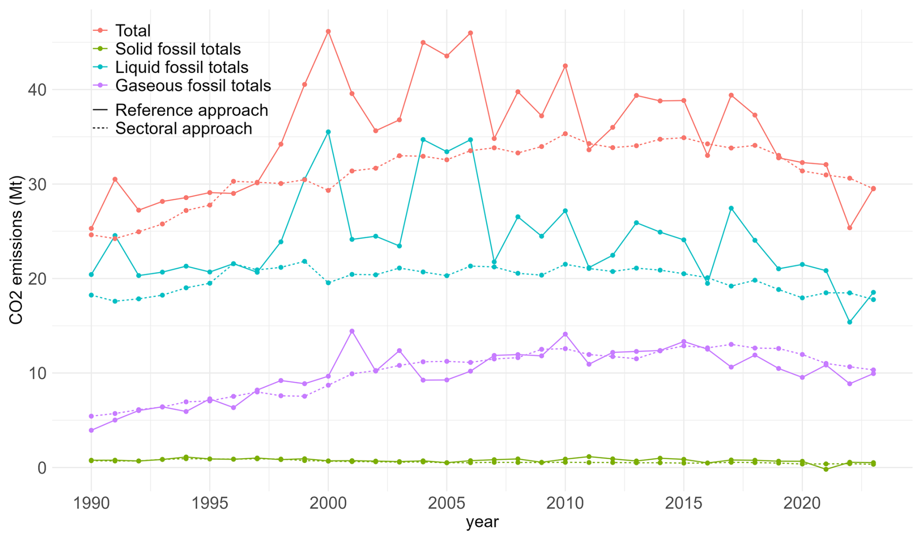
Figure K1Comparison of Norway's officially reported emissions using the reference approach and the sectoral approach reported in the CRT (Norwegian Government, 2025).
Here, we show the absolute monthly emissions estimates from the datasets compared in Sect. 3.6. As can be seen from the figure, the monthly emissions values are highly correlated (as would be expected) and are difficult to disentangle visually. Hence, in the main text we showed the relative differences of each dataset compared to our dataset.
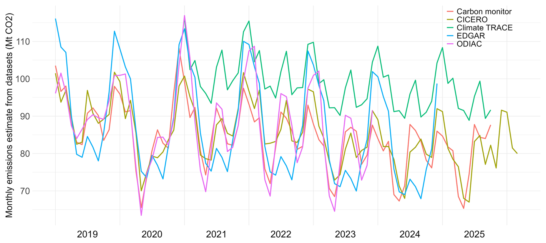
Figure L1Monthly emissions estimate with absolute value shown for all datasets. CICERO refers to the dataset from our study.
We summarize the emissions scope (including sectors included) of the datasets compared in Sect. 3.6. Details are in the main text and the references.
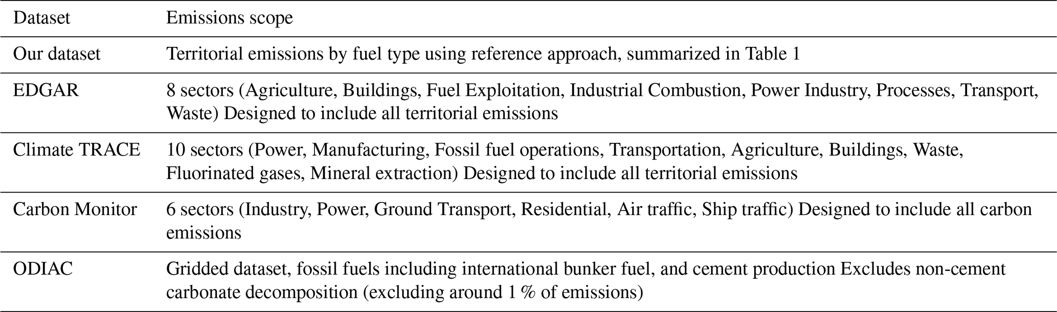
Both authors conceptualized and designed the study, processed the data, carried out the analysis, produced the figures and prepared the manuscript.
The contact author has declared that neither of the authors has any competing interests.
Publisher's note: Copernicus Publications remains neutral with regard to jurisdictional claims made in the text, published maps, institutional affiliations, or any other geographical representation in this paper. The authors bear the ultimate responsibility for providing appropriate place names. Views expressed in the text are those of the authors and do not necessarily reflect the views of the publisher.
We gratefully acknowledge funding from the Norwegian Environment Agency (agreement 24012076) and internal funding from CICERO Center for International Climate Research.
This research has been supported by the Norwegian Environment Agency (agreement 24012076) and internal funding from CICERO Center for International Climate Research.
This paper was edited by Bo Zheng and reviewed by two anonymous referees.
Andres, R. J., Gregg, J. S., Losey, L., Marland, G., and Boden, T. A.: Monthly, global emissions of carbon dioxide from fossil fuel consumption, Tellus B, 63, 309–327, https://doi.org/10.1111/j.1600-0889.2011.00530.x, 2011.
Andrew, R. M.: Timely estimates of India's annual and monthly fossil CO2 emissions, Earth Syst. Sci. Data, 12, 2411–2421, https://doi.org/10.5194/essd-12-2411-2020, 2020.
Andrew, R. M.: Towards near real-time, monthly fossil CO2 emissions estimates for the European Union with current-year projections, Atmos. Pollut. Res., 12, 101229, https://doi.org/10.1016/j.apr.2021.101229, 2021.
Andrew, R. M.: Monthly Japanese trade data December 1998 to December 2008 (extracted from PDFs) (250228), Zenodo [data set], https://doi.org/10.5281/ZENODO.14944141, 2025.
Australian Government: National Inventory Report 2023, https://unfccc.int/documents/647190 (last access: 1 November 2026), 2025.
Blasing, T. J., Broniak, C. T., and Marland, G.: The annual cycle of fossil-fuel carbon dioxide emissions in the United States, Tellus B, 57, 107–115, https://doi.org/10.3402/tellusb.v57i2.16779, 2005.
Brinkerink, M., Gallachóir, B. Ó., and Deane, P.: Building and Calibrating a Country-Level Detailed Global Electricity Model Based on Public Data, Energy Strateg. Rev., 33, 100592, https://doi.org/10.1016/j.esr.2020.100592, 2021.
Calvo Buendia, E., Tanabe, K., Kranjc, A., Baasansuren, J., Fukuda, M., Ngarize, S., Osako, A., Pyrozhenko, Y., Shermanau, P., and Federici, S. (Eds.): 2019 refinement to the 2006 IPCC guidelines for national greenhouse gas inventories, IPCC, Switzerland, https://www.ipcc.ch/report/2019-refinement-to-the-2006-ipcc-guidelines-for-national-greenhouse-gas-inventories/ (last access: 1 November 2026), 2019.
Chevallier, F.: Fluxes of Carbon Dioxide From Managed Ecosystems Estimated by National Inventories Compared to Atmospheric Inverse Modeling, Geophys. Res. Lett., 48, e2021GL093565, https://doi.org/10.1029/2021GL093565, 2021.
Chevallier, F., Fisher, M., Peylin, P., Serrar, S., Bousquet, P., Bréon, F.-M., Chédin, A., and Ciais, P.: Inferring CO2 sources and sinks from satellite observations: Method and application to TOVS data, J. Geophys. Res.-Atmos., 110, D24309, https://doi.org/10.1029/2005JD006390, 2005.
Citepa: Baromètre des émissions, https://www.citepa.org/donnees-air-climat/donnees-gaz-a-effet-de-serre/barometre-des-emissions-mensuelles/ (last access: 16 October 2026), 2026.
Climate TRACE: Climate TRACE Releases First Comprehensive, Independent Database of Global Greenhouse Gas Emissions, https://www.climatetrace.org/news/climate-trace-releases-first-comprehensive-independent (last access: 16 October 2026), 2021.
Climate TRACE: Climate TRACE Emissions Inventory v5.2.0, https://climatetrace.org (last access: 1 November 2026), 2025.
Couture, H. D., Alvara, M., Freeman, J., Davitt, A., Koenig, H., Rouzbeh Kargar, A., O'Connor, J., Söldner-Rembold, I., Ferreira, A., Jeyaratnam, J., Lewis, J., McCormick, C., Nakano, T., Dalisay, C., Lewis, C., Volpato, G., Gray, M., and McCormick, G.: Estimating Carbon Dioxide Emissions from Power Plant Water Vapor Plumes Using Satellite Imagery and Machine Learning, Remote Sens., 16, 1290, https://doi.org/10.3390/rs16071290, 2024.
Crippa, M., Solazzo, E., Huang, G., Guizzardi, D., Koffi, E., Muntean, M., Schieberle, C., Friedrich, R., and Janssens-Maenhout, G.: High resolution temporal profiles in the Emissions Database for Global Atmospheric Research, Sci. Data, 7, 121, https://doi.org/10.1038/s41597-020-0462-2, 2020.
Department of Climate Change, Energy, the Environment and Water, Australian Government: National Greenhouse Gas Inventory Quarterly Update: June 2025, https://www.dcceew.gov.au/climate-change/publications/national-greenhouse-gas-inventory-quarterly-update-june-2025 (last access: 1 November 2026), 2025.
Eggleston, H. S., Buendia, L., Miwa, K., Ngara, T., and Tanabe, K. (Eds.): 2006 IPCC guidelines for national greenhouse gas inventories, Institute for Global Environmental Strategies, Hayama, Japan, https://www.ipcc-nggip.iges.or.jp/public/2006gl/ (last access: 1 November 2026), 2006.
Egyptian Government: Egypt's First Biennial Transparency Report, https://unfccc.int/documents/645200 (last access: 1 November 2026), 2025.
EIA: Short-Term Energy Outlook – Data Series Revisions (9 September 2009), https://www.eia.gov/outlooks/steo/report/changes.php (last access: 1 November 2026), 2009.
Energy Policy and Planning Office, Ministry of Energy, Thailand: CO2 Emission, https://www.eppo.go.th/energy-statistics/co2-statistic/ (last access: 16 October 2026), 2026.
European Commission Joint Research Centre: CO2 emissions of all world countries – JRC/IEA/PBL 2022 Report, Publications Office of the European Union, Luxembourg, https://doi.org/10.2760/730164, 2022.
European Commission Joint Research Centre: EDGAR (Emissions Database for Global Atmospheric Research) Community GHG Database, version EDGAR_2025_GHG, https://edgar.jrc.ec.europa.eu/report_2025 (last access: 1 November 2026), 2025.
Eurostat (Ed.): Handbook on quarterly national accounts, 2013 edition, Publications Office, Luxembourg, https://doi.org/10.2785/46080, 2013.
Eurostat: Quarterly greenhouse gas emissions in the EU, https://ec.europa.eu/eurostat/statistics-explained/index.php?title=Quarterly_greenhouse_gas_emissions_in_the_EU#Data_sources (last access: 16 October 2026), 2026.
Freeman, J., Kargar, A. R., Couture, H. D., Alvara, M., Christian, P., Doctor, Z., Jeyaratnam, J., Lewis, J., Koenig, H., Nakano, T., Davitt, A., Lewis, C., and McCormick, G.: Power sector: Emissions from Electricity Generation, https://github.com/climatetracecoalition/methodology-
documents/blob/b71bb619ca1ac15ef477635535f0914928aed48
7/2025/Power/Emissions%20from%20Electricity%20Generati
on-PowerSector-112025.docx.pdf (last access: 1 November 2026), 2025.
Friedlingstein, P., O'Sullivan, M., Jones, M. W., Andrew, R. M., Bakker, D. C. E., Hauck, J., Landschützer, P., Le Quéré, C., Li, H., Luijkx, I. T., Peters, G. P., Peters, W., Pongratz, J., Schwingshackl, C., Sitch, S., Canadell, J. G., Ciais, P., Aas, K., Alin, S. R., Anthoni, P., Barbero, L., Bates, N. R., Bellouin, N., Benoit-Cattin, A., Berghoff, C. F., Bernardello, R., Bopp, L., Brasika, I. B. M., Chamberlain, M. A., Chandra, N., Chevallier, F., Chini, L. P., Collier, N. O., Colligan, T. H., Cronin, M., Djeutchouang, L. M., Dou, X., Enright, M. P., Enyo, K., Erb, M., Evans, W., Feely, R. A., Feng, L., Ford, D. J., Foster, A., Fransner, F., Gasser, T., Gehlen, M., Gkritzalis, T., Goncalves De Souza, J., Grassi, G., Gregor, L., Gruber, N., Guenet, B., Gürses, Ö., Harrington, K., Harris, I., Heinke, J., Hurtt, G. C., Iida, Y., Ilyina, T., Ito, A., Jacobson, A. R., Jain, A. K., Jarníková, T., Jersild, A., Jiang, F., Jones, S. D., Kato, E., Keeling, R. F., Klein Goldewijk, K., Knauer, J., Kong, Y., Korsbakken, J. I., Koven, C., Kunimitsu, T., Lan, X., Liu, J., Liu, Z., Liu, Z., Lo Monaco, C., Ma, L., Marland, G., McGuire, P. C., McKinley, G. A., Melton, J. R., Monacci, N., Monier, E., Morgan, E. J., Munro, D. R., Müller, J. D., Nakaoka, S.-I., Nayagam, L. R., Niwa, Y., Nutzel, T., Olsen, A., Omar, A. M., Pan, N., Pandey, S., Pierrot, D., Qin, Z., Regnier, P., Rehder, G., Resplandy, L., Roobaert, A., Rosan, T. M., Rödenbeck, C., Schwinger, J., Skjelvan, I., Smallman, T. L., Spada, V., Sreeush, M. G., Sun, Q., Sutton, A. J., Sweeney, C., Swingedouw, D., Séférian, R., Takao, S., Tatebe, H., Tian, H., Tian, X., Tilbrook, B., Tsujino, H., Tubiello, F., van Ooijen, E., van der Werf, G. R., van de Velde, S. J., Walker, A. P., Wanninkhof, R., Yang, X., Yuan, W., Yue, X., and Zeng, J.: Global Carbon Budget 2025, Earth Syst. Sci. Data, 18, 3211–3288, https://doi.org/10.5194/essd-18-3211-2026, 2026.
Greenhouse Gas Inventory & Research Center of Korea: Q1 2025 Preliminary greenhouse gas levels in the energy sector, https://www.gir.go.kr/home/board/read.do?boardId=85&boardMasterId=2&menuId=36 (last access: 1 November 2026), 2025.
Greenhouse Gas Inventory Office of Japan and Ministry of the Environment, Japan (eds.): National Greenhouse Gas Inventory Document of JAPAN 2025, Center for Global Environmental Research, Earth System Division, National Institute for Environmental Studies, Japan, https://unfccc.int/documents/646591 (last access: 1 November 2026), 2025.
Gregg, J. S. and Andres, R. J.: A method for estimating the temporal and spatial patterns of carbon dioxide emissions from national fossil-fuel consumption, Tellus B, 60, 1–10, https://doi.org/10.1111/j.1600-0889.2007.00319.x, 2008.
Gregg, J. S., Andres, R. J., and Marland, G.: China: Emissions pattern of the world leader in CO2 emissions from fossil fuel consumption and cement production, Geophys. Res. Lett., 35, L08806, https://doi.org/10.1029/2007GL032887, 2008.
Gurney, K. R., Aslam, B., Dass, P., Gawuc, L., Hocking, T., Barber, J. J., and Kato, A.: Assessment of the Climate Trace global powerplant CO2 emissions, Environ. Res. Lett., 19, 114062, https://doi.org/10.1088/1748-9326/ad8364, 2024.
Gurney, K. R., Aslam, B., and Dass, P.: Assessing the accuracy of the Climate Trace global vehicular CO2 emissions, Environ. Res. Lett., 21, 094018, https://doi.org/10.1088/1748-9326/ae6355, 2026.
Ida, H. and Emori, S.: Analysis of TV broadcasts on Climate Change Issue in Japan, Jpn. J. Sci. Commun., 36, 17–29, https://doi.org/10.14943/112881, 2025.
IEA: Greenhouse Gas Emissions from Energy 2025 EDITION – Database documentation, https://www.iea.org/data-and-statistics/data-product/greenhouse-gas-emissions-from-energy-highlights (last access: 1 November 2026), 2025.
Japan Cement Association: Cement Handbook 2026, https://www.jcassoc.or.jp/cement/1jpn/jj3h.html (last access: 1 November 2026), 2026 (in Japanese).
Japanese Government: Japan's Nationally Determined Contribution (NDC), https://unfccc.int/NDCREG (last access: 1 November 2026), 2021.
Japanese Government: Japan's Nationally Determined Contribution (NDC), https://unfccc.int/NDCREG (last access: 1 November 2026), 2025.
Kott, T., Foster, K., Villafane-Delgado, M., Loschen, W., Sicurello, P., Ghebreselassie, M., Reilly, E., and Hughes, M.: Transportation Sector: Global Road Emissions, Climate TRACE, https://github.com/climatetracecoalition/methodology-
documents/blob/main/2024/Transportation/Transportation%20
sector-Global%20Road%20Emissions.pdf (last access: 1 November 2026), 2024.
Kunimitsu, T. and Andrew, R. M.: Monthly-updated territorial fossil CO2 emissions estimates for Japan, Zenodo [data set], https://doi.org/10.5281/zenodo.20023226, 2026.
Kurokawa, J. and Ohara, T.: Long-term historical trends in air pollutant emissions in Asia: Regional Emission inventory in ASia (REAS) version 3, Atmos. Chem. Phys., 20, 12761–12793, https://doi.org/10.5194/acp-20-12761-2020, 2020.
Le Quéré, C., Jackson, R. B., Jones, M. W., Smith, A. J. P., Abernethy, S., Andrew, R. M., De-Gol, A. J., Willis, D. R., Shan, Y., Canadell, J. G., Friedlingstein, P., Creutzig, F., and Peters, G. P.: Temporary reduction in daily global CO2 emissions during the COVID-19 forced confinement, Nat. Clim. Change, 10, 647–653, https://doi.org/10.1038/s41558-020-0797-x, 2020.
Li, M., Kurokawa, J., Zhang, Q., Woo, J.-H., Morikawa, T., Chatani, S., Lu, Z., Song, Y., Geng, G., Hu, H., Kim, J., Cooper, O. R., and McDonald, B. C.: MIXv2: a long-term mosaic emission inventory for Asia (2010–2017), Atmos. Chem. Phys., 24, 3925–3952, https://doi.org/10.5194/acp-24-3925-2024, 2024.
Liu, Z., Ciais, P., Deng, Z., Davis, S. J., Zheng, B., Wang, Y., Cui, D., Zhu, B., Dou, X., Ke, P., Sun, T., Guo, R., Zhong, H., Boucher, O., Bréon, F.-M., Lu, C., Guo, R., Xue, J., Boucher, E., Tanaka, K., and Chevallier, F.: Carbon Monitor, a near-real-time daily dataset of global CO2 emission from fossil fuel and cement production, Sci. Data, 7, 392, https://doi.org/10.1038/s41597-020-00708-7, 2020.
Liu, Z., Ciais, P., Deng, Z., Davis, S. J., Zheng, B., Wang, Y., Song, X., Cui, D., Zhu, B., Dou, X., Ke, P., Sun, T., Guo, R., Boucher, O., Bréon, F.-M., Lu, C., Guo, R., Boucher, E., Chevallier, F., Tanaka, K., and Hong, C.: Carbon Monitor, near-real time daily datasets of global and regional CO2 emissions from fossil fuel and cement production, https://docs.google.com/document/d/1_q4QSUeSbwToR5ePTJnCxUzjsZFN-DbO/edit (last access: 1 November 2026), 2025.
Maksyutov, S. and Oda, T.: The Open-source Data Inventory for Anthropogenic CO2 (ODIAC), version 2024 (ODIAC2024), https://db.cger.nies.go.jp/dataset/ODIAC/DL_odiac2024.html (last access: 1 November 2026), 2025.
Mattsson, N., Verendel, V., Hedenus, F., and Reichenberg, L.: An autopilot for energy models – Automatic generation of renewable supply curves, hourly capacity factors and hourly synthetic electricity demand for arbitrary world regions, Energy Strateg. Rev., 33, 100606, https://doi.org/10.1016/j.esr.2020.100606, 2021.
METI (Ministry of Economy, Trade and Industry): Revision and corrections to the General Energy Statistics, 21 April 2023, https://www.enecho.meti.go.jp/statistics/total_energy/review.html (last access: 1 November 2026), 2023 (in Japanese).
METI (Ministry of Economy, Trade and Industry): General Energy Statistics (FY2023), https://www.enecho.meti.go.jp/statistics/total_energy/results.html (last access: 1 November 2026), 2025.
METI (Ministry of Economy, Trade and Industry): Current Survey of Energy Consumption, https://www.enecho.meti.go.jp/statistics/energy_consumption/ec003/ (last access: 15 October 2026), 2026a.
METI (Ministry of Economy, Trade and Industry): Current Survey of Production Concerning Gas Industry, https://www.enecho.meti.go.jp/statistics/gas/ga001/index.html (last access: 15 October 2026), 2026b.
METI (Ministry of Economy, Trade and Industry): Electric Power Investigation Statistics, https://www.enecho.meti.go.jp/statistics/electric_power/ep002/ (last access: 15 ctober 2026), 2026c.
METI (Ministry of Economy, Trade and Industry): Monthly Report of Current Production Statistics, https://www.meti.go.jp/statistics/tyo/seidou/result/ichiran/08_seidou.html (last access: 15 October 2026), 2026d.
METI (Ministry of Economy, Trade and Industry): Report on Petroleum Statistics, https://www.meti.go.jp/statistics/tyo/sekiyuka/index.html (last access: 15 October 2026), 2026e.
Min, S. and Choi, Y.: Proactive Estimation of the Energy Sector GHG Emissions Using Monthly Data (Korean), Korean Energy Econ. Rev., 23, 21–48, https://doi.org/10.22794/keer.2024.23.1.002, 2024.
MOF (Ministry of Finance): Trade Statistics of Japan, https://www.customs.go.jp/toukei/info/index_e.htm (last access: 15 October 2026), 2026.
Norwegian Government: Greenhouse Gas Emissions 1990–2023 National Inventory Report, https://unfccc.int/documents/646033 (last access: 1 November 2026), 2025.
Oda, T. and Maksyutov, S.: A very high-resolution (1 km × 1 km) global fossil fuel CO2 emission inventory derived using a point source database and satellite observations of nighttime lights, Atmos. Chem. Phys., 11, 543–556, https://doi.org/10.5194/acp-11-543-2011, 2011.
Oda, T. and Maksyutov, S.: ODIAC Fossil Fuel CO2 Emissions Dataset (Version name: ODIAC2024), Center for Global Environmental Research, National Institute for Environmental Studies [data set], https://doi.org/10.17595/20170411.001, 2025.
Oda, T., Maksyutov, S., and Andres, R. J.: The Open-source Data Inventory for Anthropogenic CO2, version 2016 (ODIAC2016): a global monthly fossil fuel CO2 gridded emissions data product for tracer transport simulations and surface flux inversions, Earth Syst. Sci. Data, 10, 87–107, https://doi.org/10.5194/essd-10-87-2018, 2018.
Oda, T., Haga, C., Hosomi, K., Matsui, T., and Bun, R.: Errors and uncertainties associated with the use of unconventional activity data for estimating CO2 emissions: the case for traffic emissions in Japan, Environ. Res. Lett., 16, 084058, https://doi.org/10.1088/1748-9326/ac109d, 2021.
Office for National Statistics, UK Government: Estimates of quarterly greenhouse gas emissions (residence basis), UK: Quarter 3 (July to September) 2025, https://www.ons.gov.uk/economy/environmentalaccounts/
bulletins/experimentalestimatesofquarterlygreenhousegasemissi
onsresidencebasisuk/quarter3julytoseptember2025 (last access: 1 November 2026), 2026.
Ohyama, H., Frey, M. M., Morino, I., Shiomi, K., Nishihashi, M., Miyauchi, T., Yamada, H., Saito, M., Wakasa, M., Blumenstock, T., and Hase, F.: Anthropogenic CO2 emission estimates in the Tokyo metropolitan area from ground-based CO2 column observations, Atmos. Chem. Phys., 23, 15097–15119, https://doi.org/10.5194/acp-23-15097-2023, 2023.
Pakistani Government: Pakistan's Biennial Transparency Report (BTR), https://unfccc.int/documents/645241 (last access: 1 November 2026), 2025.
Stats NZ, New Zealand Government: Greenhouse gas emissions (industry and household): December 2025 quarter, https://www.stats.govt.nz/information-releases/greenhouse-gas-emissions-industry-and-household-december-2025-quarter/ (last access: 1 November 2026), 2026.
Steinstraeter, M., Heinrich, T., and Lienkamp, M.: Effect of Low Temperature on Electric Vehicle Range, World Electr. Veh. J., 12, 115, https://doi.org/10.3390/wevj12030115, 2021.
UNFCCC: Guidelines for the technical review of information reported under the Convention related to greenhouse gas inventories, biennial reports and national communications by Parties included in Annex I to the Convention. Decision 13/CP.20, FCCC/CP/2014/10/Add.3, https://unfccc.int/documents/8613 (last access: 1 November 2026), 2015.
Urraca, R., Janssens-Maenhout, G., Álamos, N., Berna-Peña, L., Crippa, M., Darras, S., Dellaert, S., Denier van der Gon, H., Dowell, M., Gobron, N., Granier, C., Grassi, G., Guevara, M., Guizzardi, D., Gurney, K., Huneeus, N., Keita, S., Kuenen, J., Lopez-Noreña, A., Puliafito, E., Roest, G., Rossi, S., Soulie, A., and Visschedijk, A.: CoCO2-MOSAIC 1.0: a global mosaic of regional, gridded, fossil, and biofuel CO2 emission inventories, Earth Syst. Sci. Data, 16, 501–523, https://doi.org/10.5194/essd-16-501-2024, 2024.
Worland, J.: How a New Effort to Trace Emissions, Led by Al Gore, Could Reshape Climate Talks, Time Magazine, https://time.com/5866881/al-gore-climate-trace-emissions/ (last access: 1 November 2026), 2020.
Xu, R., Tong, D., Xiao, Q., Qin, X., Chen, C., Yan, L., Cheng, J., Cui, C., Hu, H., Liu, W., Yan, X., Wang, H., Liu, X., Geng, G., Lei, Y., Guan, D., He, K., and Zhang, Q.: MEIC-global-CO2: A new global CO2 emission inventory with highly-resolved source category and sub-country information, Sci. China Earth Sci., 67, 450–465, https://doi.org/10.1007/s11430-023-1230-3, 2024.
Parts of the fuels categorized as non-energy usage do result in oxidation outside the energy sector, for example petroleum coke use for ammonia production, and coal tar use for carbon black production. These emissions are separately covered in the industrial processes category in the CRT, although not included in the current monthly dataset construction due to their small contribution, as described in Sect. 3.5.1.
While for most fuels the total of all industries gives the non-energy usage value, for several fuels this has duplication due to some companies registering in multiple industry sectors. This is the case for LPG, Coke oven/gas coke, and Coal tar. The guideline for the General Energy Statistics notes this as a general point, but which specific industry each fuel needs to refer to needs to be checked by comparing to the annual data.
The emissions factor per limestone (calcium carbonate) weight is 0.428, which is the value that appears in the CRT. This can be converted to the per-lime weight factor by .
- Abstract
- Introduction
- Methods and data
- Results
- Data availability
- Discussion
- Appendix A: Detailed description of input data
- Appendix B: Linear disaggregation of annual data into monthly data
- Appendix C: Naphtha non-energy usage data
- Appendix D: Analysis of EDGAR's temporal profiles
- Appendix E: Climate TRACE methodology change in the power sector
- Appendix F: Carbon Monitor methodology change in the ground transportation sector
- Appendix G: Territorial emissions and economic activity-based emissions in Ireland
- Appendix H: Conversion factor for natural gas production data
- Appendix I: Revisions in reported CO2 emissions
- Appendix J: X-11 method
- Appendix K: Comparison of sectoral approach emissions and reference approach emissions for Norway
- Appendix L: Monthly emissions estimate comparison with other datasets
- Appendix M: Summary table of dataset characteristics
- Author contributions
- Competing interests
- Disclaimer
- Acknowledgements
- Financial support
- Review statement
- References
- Abstract
- Introduction
- Methods and data
- Results
- Data availability
- Discussion
- Appendix A: Detailed description of input data
- Appendix B: Linear disaggregation of annual data into monthly data
- Appendix C: Naphtha non-energy usage data
- Appendix D: Analysis of EDGAR's temporal profiles
- Appendix E: Climate TRACE methodology change in the power sector
- Appendix F: Carbon Monitor methodology change in the ground transportation sector
- Appendix G: Territorial emissions and economic activity-based emissions in Ireland
- Appendix H: Conversion factor for natural gas production data
- Appendix I: Revisions in reported CO2 emissions
- Appendix J: X-11 method
- Appendix K: Comparison of sectoral approach emissions and reference approach emissions for Norway
- Appendix L: Monthly emissions estimate comparison with other datasets
- Appendix M: Summary table of dataset characteristics
- Author contributions
- Competing interests
- Disclaimer
- Acknowledgements
- Financial support
- Review statement
- References