META4.0: a new global mesoscale eddy network atlas derived from altimetry

This study introduces the new global Mesoscale Eddy Trajectory Atlases, META4.0 available in an AVISO repository at https://doi.org/10.24400/527896/a01-2026.001 (CLS and CNES, 2026). META4.0 provides eddy detections, trajectories, and interaction networks derived from satellite altimetry. Eddy detection relies on the pyeddytracker (PET) algorithm (Mason et al., 2014), further optimized by Pegliasco et al. (2022), and represents a substantial improvement over the previous META3.2 product (SSALTO/DUACS, distributed by AVISO+ with CNES support).

The main advance of META4.0 is the explicit identification of eddy merging and splitting events. By combining grouping, which links detections across consecutive days, and segmentation, which tracks continuity through interaction events, trajectories are organized into networks of interconnected eddies. This network-based representation complements the single-trajectory view of eddy life cycles by explicitly accounting for eddy interactions.

The paper presents both diagnostic tools designed to explore individual eddy networks (e.g., timelines, spatial trajectories, and eddy properties such as effective radius or shape error) and the results of a global statistical analysis over more than three decades. These tools and analyses offer new diagnostics for investigating network properties, eddy lifetimes, and the spatial and temporal distribution of merging and splitting events of the META4.0 atlas. Clustering analyses reveal recurrent interaction patterns and identify regions where eddy networks are particularly active. An independent dataset of surface chlorophyll concentration is used for qualitative validation of selected events. Finally, Lagrangian advection of synthetic particles highlights coherent forward and backward transport signatures associated with interaction events, providing a physical validation of the reconstructed networks.

Overall, META4.0 offers a novel and physically consistent framework to characterize mesoscale eddy interactions and to better understand their role in shaping ocean dynamics.

1 Introduction

1.1 General context

Mesoscale eddies are key drivers of ocean dynamics, playing a central role in the transport of water masses, energy, heat, salt, and biogeochemical tracers across both horizontal and vertical scales. These ubiquitous structures, typically spanning tens to hundreds of kilometers and persisting from days to several years (Morrow and Le Traon, 2012), also exert a strong influence on marine biological and chemical processes (Beal et al., 2011; Chaigneau et al., 2011; Gaube et al., 2014; Gruber et al., 2011; Sosa-Gutierrez et al., 2025; Zhang et al., 2014). Coupling eddy-resolving physical observations with ecological datasets has substantially advanced our understanding of marine animal behavior (Braun et al., 2019; Chambault et al., 2019; Christie et al., 2010; Siegel et al., 2008; Staaterman et al., 2012) as well as the dispersion and fate of pollutants (Brach et al., 2018; Gilchrist et al., 2020). Continuous improvements in the accuracy of satellite altimetry over the past three decades have enabled global monitoring of mesoscale eddies, providing unprecedented insights into their role in ocean circulation and ecosystem functioning.

1.2 Eddy detection and atlases

Satellite altimetry provides near-global, weather-independent observations of mesoscale ocean variability, primarily through daily, multi-satellite gridded fields of absolute dynamic topography (ADT) and sea level anomaly (SLA). Although the spatiotemporal interpolation of nadir altimeter observations limits the effective resolution of these gridded products to spatial scales larger than ∼ 100 km, they remain the backbone of global mesoscale eddy detection. Traditionally, eddy detection methods have relied on Eulerian approaches,based on fixed, time-invariant surface fields, using either geometric diagnostics (Chaigneau et al., 2008, 2009; Faghmous et al., 2013; Ioannou et al., 2017; Liu et al., 2016) or rotational metrics (Isern-Fontanet et al., 2003; Le Vu et al., 2018; Mkhinini et al., 2014; Morrow et al., 2004; Nencioli et al., 2010). Over the past decade, Lagrangian approaches, based on time-evolving surface fields, have also been introduced (Abernathey and Haller, 2018; Beron-Vera et al., 2008; El Aouni, 2021; Haller, 2016). However, their application at the global scale remains computationally intensive.

Several global atlases have been developed, beginning with the pioneering work of Chelton et al. (2011), which was later refined through collaborations between OSU, CLS, and CNES, leading to the Mesoscale Eddy Trajectory Atlas (META; Pegliasco et al., 2022). Successive releases (META1.0exp, META2.0, META3.1exp, META3.2) progressively improved detection and tracking by refining search schemes, handling missing eddies, and extending coverage to coastal and island regions. These efforts established META as a reference global product, freely distributed via AVISO+ (https://data.aviso.altimetry.fr/aviso-gateway/data/META3.1exp_DT/, last access: 23 September 2026). Other datasets followed similar principles, such as the global atlas by Tian et al. (2020), GOMEAD (Dong et al., 2022), and ToEddies (Ioannou et al., 2024), offering complementary approaches to eddy detection and tracking.

1.3 Single-trajectory approaches

Most global atlases, including META and others (Chelton et al., 2011; Tian et al., 2020; Dong et al., 2022), rely on single-trajectory tracking, where eddies are followed over time by identifying candidates within a localized search window. The META2.0 version refined this method to handle the “missing eddy” problem through short temporal extrapolations and virtual eddies. Later versions (i.e., META3.x) adopted a contour-overlap strategy, linking detections across timesteps when their intersection exceeded a given threshold (Keppler et al., 2018; Laxenaire et al., 2018; Li et al., 2016; Pegliasco et al., 2015, 2022). This approach proved more robust, enabling consistent trajectories even during partial occlusion or deformation, and reducing the need for virtual eddies.

1.4 Eddy networks and interactions

Eddies were initially viewed as isolated coherent structures driven by baroclinic instabilities or topographic forcing (Stammer and Wunsch, 1999). However, observational and modeling evidence has revealed that mesoscale dynamics also involve frequent eddy–eddy interactions such as merging and splitting (Fang and Morrow, 2003; Adcock and Marshall, 2000; Trieling et al., 2005; Han et al., 2025; Wang et al., 2019). These processes are now recognized as a fundamental component of oceanic energy transfer and water mass transport.

Recent algorithms have been developed to explicitly identify such interactions, treating eddies as nodes within a dynamic network rather than independent trajectories. Examples include AMEDA (Le Vu et al., 2018), which integrates merging/splitting detection into tracking, the multicore Gaussian approach of Cui et al. (2019), the graph-based framework of ToEddies (Ioannou et al., 2024; Laxenaire et al., 2018, 2020), and the topological tree approach of EddyGraph (Tian et al., 2021). Together, these methods have demonstrated the potential of network-based descriptions to capture the full complexity of eddy life cycles.

1.5 The META4.0 atlas

Building upon this progress, we present the META4.0 atlas, the new global version of the Mesoscale Eddy Trajectory Atlas distributed by AVISO+. META4.0 introduces eddy networks into the dataset, providing a unified representation of eddy evolution, merging, and splitting events. This update represents a key advancement for the META eddy products, ensuring continuity with previous versions while adding a new dimension for studying eddy connectivity and interactions. As mentioned in Sect. 1.3, previous versions of the META atlas relied on a single-trajectory tracking approach, whereas META4.0 provides a network-based representation of eddy trajectories. It should be noted that the META4.0 eddy detection framework is identical to that used in the previous META3.2 version.

The construction of the networks follows three stages:

• Daily eddy detection from DT2021 ADT fields;

• Network grouping based on eddy overlap between consecutive days, accounting for missing detections;

• Network segmentation to identify merging and splitting events within each group.

Beyond the methodological improvement, the increasing complexity of network representations requires appropriate tools for data manipulation, visualization, and analysis. For this reason, the full Python source code is released under a GPL v3 license (https://doi.org/10.5281/zenodo.7197432, Delepoulle et al., 2022) and integrated into the open-source pyeddytracker (PET) library (Delepoulle et al., 2022; Mason et al., 2014; Pegliasco et al., 2022). The toolbox is freely available and documented online (https://py-eddy-tracker.readthedocs.io/en/latest/python_module/index.html, last access: 23 September 2026), providing ready-to-use functionalities for detecting eddies, analyzing trajectories, building networks, and reproducing the results presented in this paper.

This paper is organized as follows. Section 2 introduces the META4.0 algorithm and describes the data sources used. Section 3 presents the toolbox and main validation diagnostics. Section 4 details data and code availability, and Sect. 5 concludes with a summary and perspectives.

2 Data and methods

2.1 Eddy detection

2.1.1 Altimetric fields for eddy detection

Following Pegliasco et al. (2022), the detection is performed on the absolute dynamic topography (ADT) field rather than on the sea level anomaly (SLA), as done in earlier META versions. Using ADT provides better detection in dynamically energetic regions characterized by strong sea surface height (SSH) gradients or recurrent mesoscale structures such as current retroflections, coastal eddies, and topographic recirculations. Many of these features are imprinted in the mean dynamic topography (MDT), and would therefore be partially masked in SLA fields. The ADT fields used here are the global daily products from the DT2021 reprocessing (Faugère et al., 2022), with a $\mathrm{1}/\mathrm{4}$° grid resolution and corresponding to the all-satellite (all-sat) configuration and covering the 1993–2021 period. The effective resolution of the altimetric product influences the detection of eddies and their interactions, with smaller and shorter-lived features being more difficult to resolve and therefore potentially underrepresented in the resulting networks. Consequently, some merging and splitting events involving small-scale structures may not be fully captured. The present atlas is based on the DT2021 $\mathrm{1}/\mathrm{4}$° reprocessing in order to ensure consistency with the META3.2 atlas and to perform comparisons of the tracking methodologies (see Sect. 3.2.2). A new version based on the DT2024 reprocessing at $\mathrm{1}/\mathrm{8}$° resolution is currently under development and is expected to improve the representation of smaller-scale eddies and their interactions.

Unlike early approaches such as Chelton et al. (2007), which relied on the Okubo–Weiss parameter to isolate rotational structures from a non-rotative background, spatial filtering to the ADT fields is no longer applied. Filtering was originally introduced to reduce large-scale gradients and noise that affected vorticity-based methods. However, the contour-based approach adopted here is inherently less sensitive to background flow variations, as it directly identifies closed SSH contours enclosing extrema. Furthermore, sensitivity experiments indicated that spatial filtering can locally alter the geometry of SSH contours and occasionally lead to the detection of large structures that are not supported by the independently observed circulation patterns. In line with the methodology of Ioannou et al. (2024) (ToEddies), we therefore retain the full, unfiltered ADT signal, preserving the complete range of observed altimetric variability and ensuring a more faithful representation of mesoscale and submesoscale dynamics.

2.1.2 Detecting mesoscale eddies

The detection algorithm is based on the pyeddytracker (PET) software (Mason et al., 2014), itself derived from the methods of Chelton et al. (2011), Kurian et al. (2011), Penven et al. (2005). It proceeds as follows:

1. SSH contour extraction: closed contours are traced around SSH extrema with a 2 mm step as in META3.2, downward from maxima for anticyclones, upward from minima for cyclones.

2. Validation tests: each contour must

   • contain a single extremum;

   • enclose between 4 and 1000 pixels;

   • exceed an SSH amplitude of 0.4 cm;

   • have a shape error below 70 %. Following Pegliasco et al. (2022), the shape error is defined as the normalized areal difference between the contour and its best-fit circle. This criterion excludes highly irregular non-rotating structures while allowing elongated eddies associated with energetic flows and eddy interactions.

3. Interpolation and diagnostics: validated contours and mean radial speed profiles are interpolated over 30 points using the visvalingam algorithm as in META3.2 (Visvalingam, 2016)

The resulting daily detections of anticyclonic and cyclonic eddies are stored separately in NetCDF files.

2.2 Network grouping

Network construction is performed separately for anticyclonic and cyclonic eddies. While cyclonic–anticyclonic interactions do exist (Amores et al., 2017; Chang and Park, 2015; Shi and Nof, 1993), they are comparatively rare and involve complex dynamical processes. Restricting the analysis to eddies of the same polarity allows for a more robust and computationally tractable description of eddy interactions, while retaining the dominant merging and splitting dynamics observed globally.

The grouping step links daily detections into spatio-temporal networks based on their geometric overlap across consecutive days. Two eddies are connected if their intersection-over-union (IoU) overlap score O exceeds 10 %, as defined (Pegliasco et al., 2022):

$$\begin{array}{}\text{(1)}& O({\mathrm{eddy}}_{\mathrm{ref}},{\mathrm{eddy}}_{\mathrm{study}})={\displaystyle \frac{\mathrm{Area}({\mathrm{eddy}}_{\mathrm{ref}}\cap {\mathrm{eddy}}_{\mathrm{study}})}{\mathrm{Area}({\mathrm{eddy}}_{\mathrm{ref}}\cup {\mathrm{eddy}}_{\mathrm{study}})}}.\end{array}$$

In addition, a hybrid criterion is used to retain configurations for which the area of the smaller contour is almost entirely included within the larger contour, even when the IoU overlap ratio defined above falls below the threshold.

To account for occasional missing detections, resulting from mapping limitations or temporary detection failures, the search is extended up to seven days forward. This allows eddies belonging to the same trajectory to be reconnected when intermediate detections are missing. No constraint is imposed on radius or amplitude variations, allowing the detection of rapid size changes associated with merging or splitting.

These tracking parameters were selected empirically based on extensive expert evaluation of trajectory continuity and network consistency. They build upon the methodology developed for previous versions of the META atlas Pegliasco et al. (2022), while being adjusted to improve the identification of merging and splitting events in the network framework. In particular, the temporal search window was extended from 5 d in META3.2 to 7 d in META4.0. Indeed, merging and splitting events are often associated with deformations of the eddy contours and rapid changes in their properties (see Sect. 3.3.3), which can increase the occurrence of temporary detection gaps. A longer temporal window therefore improves the reconnection of eddies belonging to the same network while remaining short enough to limit spurious associations. It should however be noted that the selected overlap threshold (10 %) and temporal search window (7 d) are empirical choices and their influence on the resulting network statistics has not yet been systematically evaluated through dedicated sensitivity analyses. While the extended search window helps reduce trajectory fragmentation caused by temporary detection gaps, it may also increase the likelihood of reconnecting unrelated eddy structures, particularly in regions characterized by high eddy density, mapping uncertainties, or short-lived spurious detections. Consequently, some aspects of the reconstructed network topology, trajectory lifetimes, and merging/splitting statistics may depend on the selected parameter values.

It should be added that the complete workflow is implemented in the open-source pyeddytracker library, which allows users to modify the tracking parameters and generate customized eddy trajectories, networks, and associated statistics according to their specific applications.

The process can be summarized as follows:

• 1.

  Preprocessing of files

  • Input daily eddy detections (polygons) are sorted chronologically;

  • Missing days are checked to ensure temporal continuity.

• 2.

  Pairwise comparison across days

  • For each day, all eddies are compared with those of subsequent days within a temporal window (i.e., the next 7 d);

  • Candidate pairs are first filtered using bounding box intersection to quickly eliminate eddies that are too far apart;

  • For the remaining pairs, the geometric overlap between polygons is computed. If the normalized overlap exceeds a threshold (i.e., 10 %), the two eddies are considered connected.

• 3.

  Group construction

  • Each set of linked detections defines a group (a temporal network of eddies);

  • If a new match connects two existing groups, they are merged into a single group.

Each eddy observation is thus assigned to a group, corresponding either to a simple trajectory or to a more complex network involving multiple interacting eddies. These steps are illustrated through dedicated Jupyter notebooks available in the documentation (https://py-eddy-tracker.readthedocs.io/en/latest/python_module/16_network/pet_group_anim.html#sphx-glr-python-module-16-network-pet-group-anim-py, last access: 23 September 2026).

2.3 Network segmentation

The segmentation step decomposes each group into coherent trajectory segments bounded by an event. An event can be a birth, death, merging, or splitting, defining the start or end of one or several eddy segments. Figure 1 illustrates an example of a network composed of three segments connected through two successive events. The first segment is composed of four observed eddies represented by the dots. It ends by merging with the second observations of segment 2 resulting in a larger eddy belonging to segment 2. The fifth observation of this segment splits and gives birth to the third segment.

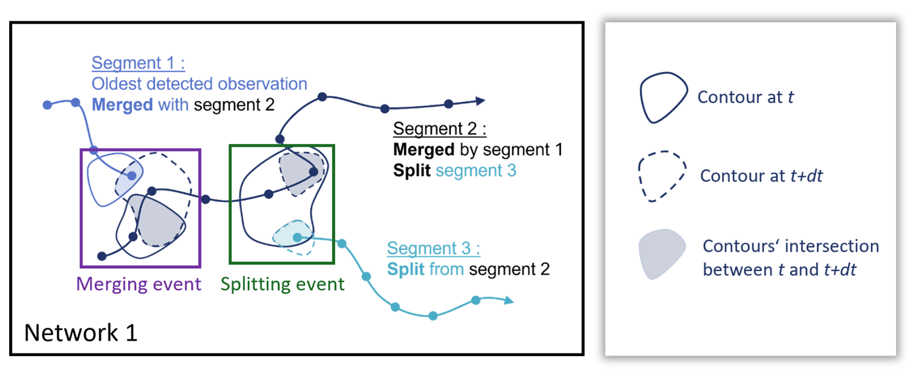
Figure 1 Example of a network composed of three segments linked by two successive events (merging and splitting).

The segmentation algorithm proceeds as follows:

• 1.

  Initialization

  • Each observation in a group is assigned an identifier and a time index;

  • Links to potential predecessors and successors are initialized.

• 2.

  Forward and backward association

  • Starting from an observation, the algorithm searches for its most likely successor in the following days (up to a window of tolerance for missing detections), based on maximal polygon overlap;

  • Similarly, the best predecessor is searched in earlier days;

  • This creates chains of linked observations, each chain defining a segment.

• 3.

  Event handling

  • Birth: observations without a predecessor → start of a new segment;

  • Death: observations without a successor → end of a segment;

  • Splitting: one observation links to multiple successors → trajectory bifurcation into several segments;

  • Merging: multiple observations link to the same successor → trajectories converge, one segment continues while others terminate;

  • Segment reindexing: when a merging or splitting event occurs, segment identifiers are reassigned to preserve continuity along the main trajectory. The branch exhibiting the largest overlap with the parent segment is considered the continuation of the trajectory and retains the original segment identifier. In a splitting event, secondary branches are assigned new identifiers, whereas in a merging event, the non-primary branch terminates. This procedure ensures that segment identities are determined by geometric continuity rather than by the order in which observations are processed.

• 4.

  Postprocessing

  • Short segments (i.e., less than 3 observations) that don't connect several segments are removed from their networks and treated as isolated features. These segments generally correspond to brief separations that are unlikely to represent robust interaction events. By contrast, short segments that connect multiple branches are retained because they contribute to the network topology and may represent genuine merging or splitting events.

• 5.

  Output

  • Each group is segmented into individual segments, capturing the full life cycle of eddies, including births, deaths, splits, and merges.

It should be noted that the segmentation algorithm does not impose any restriction on the number of eddies involved in merging or splitting events. Consequently, the resulting network topology is not limited to pairwise interactions: more than two eddies may merge into a single segment, and a single segment may split into multiple offspring segments. This design choice avoids introducing a priori constraints on the network structure and allows the atlas to represent all interaction patterns identified by the tracking algorithm.

The segmentation procedure is illustrated in the PET documentation notebooks (https://py-eddy-tracker.readthedocs.io/en/latest/python_module/16_network/ pet_segmentation_anim.html#sphx-glr-python-module-16-network-pet-segmentation-anim-py, last access: 23 September 2026), which provide visual examples and interactive tools for reproducing this step.

3 Results

In this section, the results of eddy networks detections and characterizations are presented. First, the diagnostic tools available for exploring individual networks are introduced, before moving to a global statistical analysis over three decades of data. Then, a focus is made on the dynamics of merging and splitting events, studying their spatial and temporal distributions, as well as the eddies properties during such events, and finally qualitatively validate the results with independent oceanographic observations (i.e., chlorophyll products). Eventually, the typology of networks are explored through clustering.

3.1 Exploratory tools for network analysis

In this section, the capabilities of the pyeddytracker toolbox are illustrated through a representative case study. This local example highlights some of the graphical diagnostics available to investigate the structure and dynamics of individual eddy networks.

A single network was selected from the META4.0 anticyclonic networks atlas to demonstrate the diagnostic possibilities. Networks can be extracted using flexible selection tools:

• Spatio-temporal criteria (e.g., specifying a time window and/or longitude–latitude box);

• Intrinsic characteristics such as network size or lifetime;

• Targeted searches, where the user tracks the history of a specific eddy of interest.

The chosen network characteristics are summarized in Table 1.

Table 1 Internal characteristics of the demo network.

The temporal evolution of the network is represented as timelines in Fig. 2. Timelines can be ordered either by segment identifiers or by latitude, both as a function of time. Merging and splitting events are symbolized by black hexagons and stars, respectively. Such representations are useful for quickly assessing the internal complexity of a network: the number of coexisting segments, their relative durations, and the timing of interaction events.

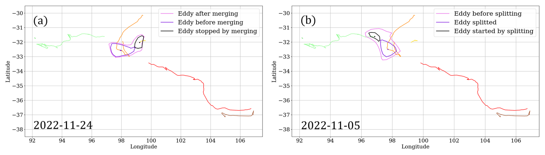
To complement this view, a geographical view of the segments is shown in Fig. 3. In this map-based representation, the merging and splitting events are explicitly localized, allowing for a joint spatial and temporal understanding of network dynamics.

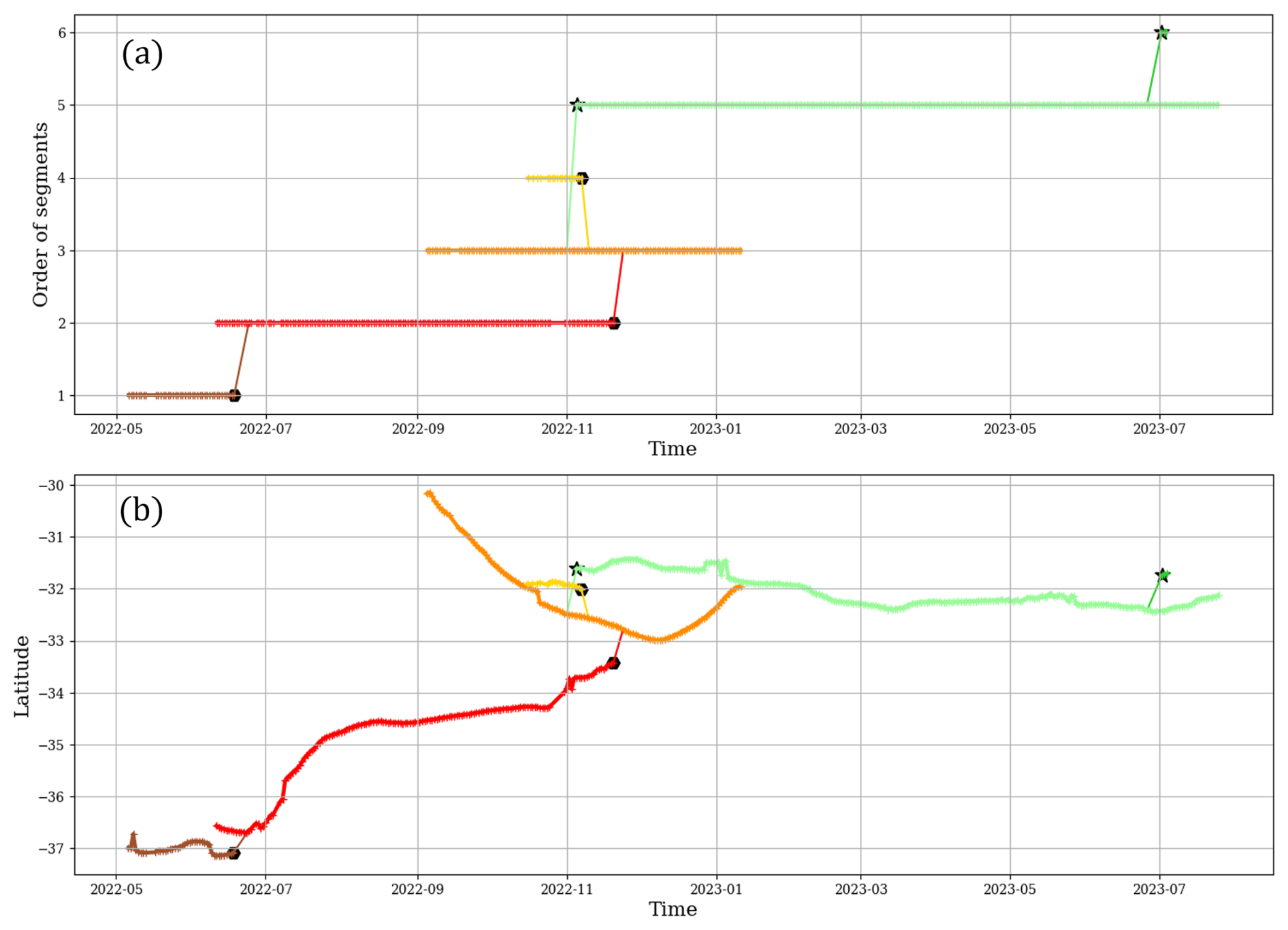
Figure 2 Timelines of the demo network (a) function of the segment identifiers (b) function of latitude. Hexagons: merging events. Stars: splitting events.

Figure 3 Demo networks segments' tracks and (a) merging (b) splitting events.

Timelines can also be enriched with eddy properties such as effective radius or shape error, as illustrated in Fig. 4. On this timeline, each dot corresponds to an observed eddy. Marker color indicates the shape error, while marker size is proportional to the effective radius. This combined representation directly links the temporal organization of eddy segments to the evolution of their physical characteristics.

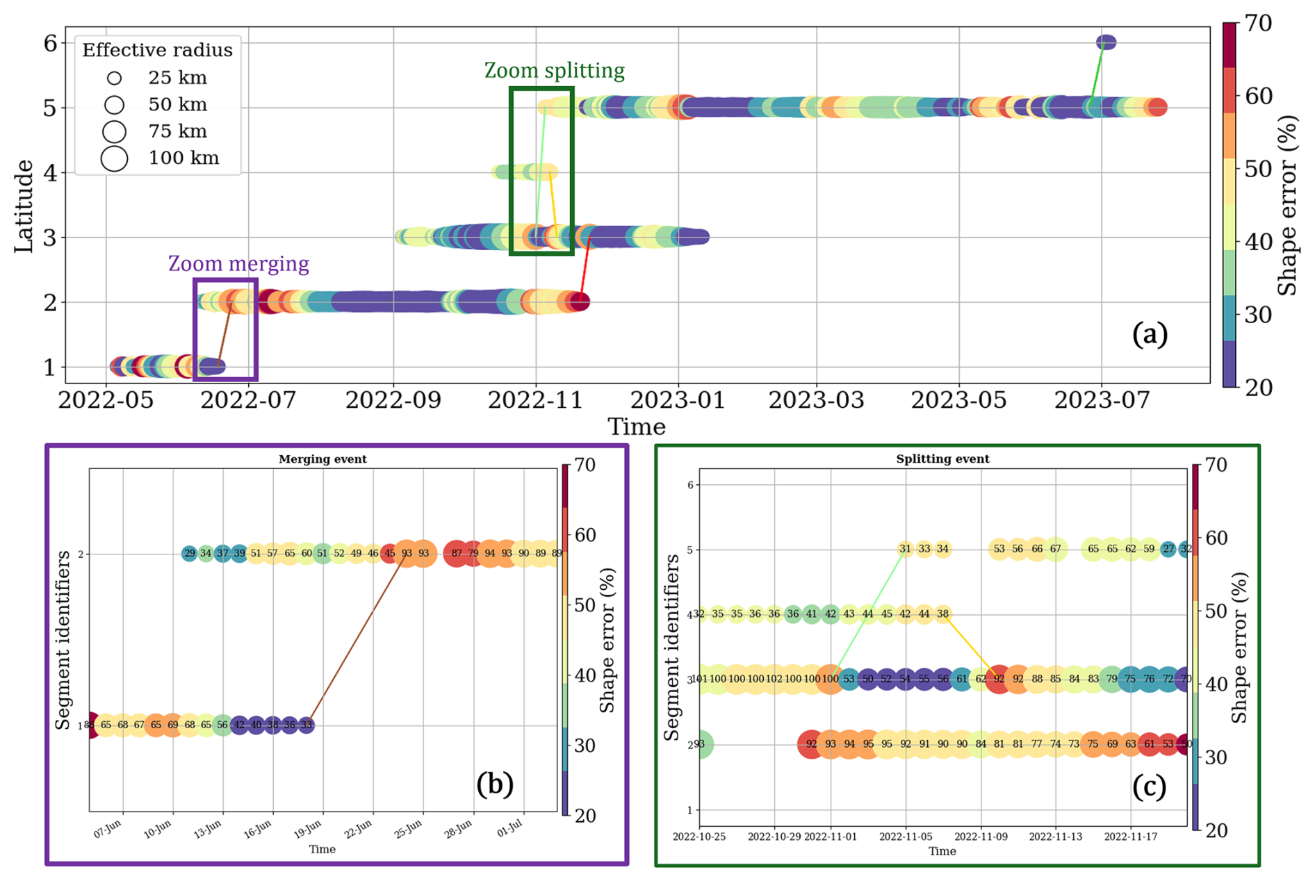
Figure 4 Timeline representation of the selected network. (a) Complete network evolution. (b) Detailed view of the merging event between segments 1 and 2. (c) Detailed view of the splitting event occurring later in the network evolution. A merging event is also visible. Marker size is proportional to the effective radius (also indicated numerically in kilometers) and color indicates the shape error.

For example, Fig. 4 reveals that the effective radius tends to increase after merging events and before splitting events, suggesting a reorganization of the eddy structure when mass and energy are redistributed. At the same time, the timeline indicates that eddies become more distorted around interaction events, corresponding to increased dynamic stress during merging or division. Together, these diagnostics provide physically interpretable signatures of merging and splitting: growth in size accompanied by shape deformation is a strong indicator of structural reorganization. Similar diagnostics could also be performed with other eddy properties such as amplitude or mean translation speed, however, they are omitted here for conciseness.

Overall, these diagnostics can be particularly informative for:

• Detecting structural changes in eddy properties (e.g., increase in radius, deformation) around merging and splitting events;

• Tracing the continuity of segments and checking whether apparent gaps in detection correspond to real interruptions or short-lived tracking issues;

• Visually linking eddy trajectories with interaction events to assess the temporal ordering of merging and splitting within a network.

These exploratory diagnostics therefore provide a practical toolkit for investigating the structure and dynamics of individual eddy networks. While they are demonstrated here on a single representative case, the tendencies observed will be assessed and statistically confirmed at the global scale in the following sections.

3.2 Global statistics

3.2.1 General information

The main properties of the META4.0 dataset are summarized in Table 2. These numbers provide a first overview of the database, including the total number of eddy observations, the number of reconstructed networks and segments, and the occurrence of merging and splitting events. For completeness, the number of lonely eddies (i.e., eddies that were never associated with any network) is also reported.

Table 2 Global characteristics of the META4.0 dataset. AC: Anticyclonic eddies global atlas. C: cyclonic eddies global atlas. AC+C: META4.0 global atlas.

The lonely eddies correspond to individual eddies that could not be attached to any trajectory or network. Their spatial distribution is shown in Fig. 5, expressed as the number of lonely eddy detections per year and per degree², in 0.25° boxes. This diagnostic reveals that lonely eddies occur throughout the global ocean, but with enhanced frequencies in specific regions: along continental slopes and coasts (e.g., the Indonesian seas), at high and low latitudes (e.g., the Bering Strait), and within the equatorial band (e.g., the western Pacific). These patterns are consistent with areas where mesoscale detection is more challenging, either because of energetic small-scale variability, proximity to land, or reduced altimetric resolution.

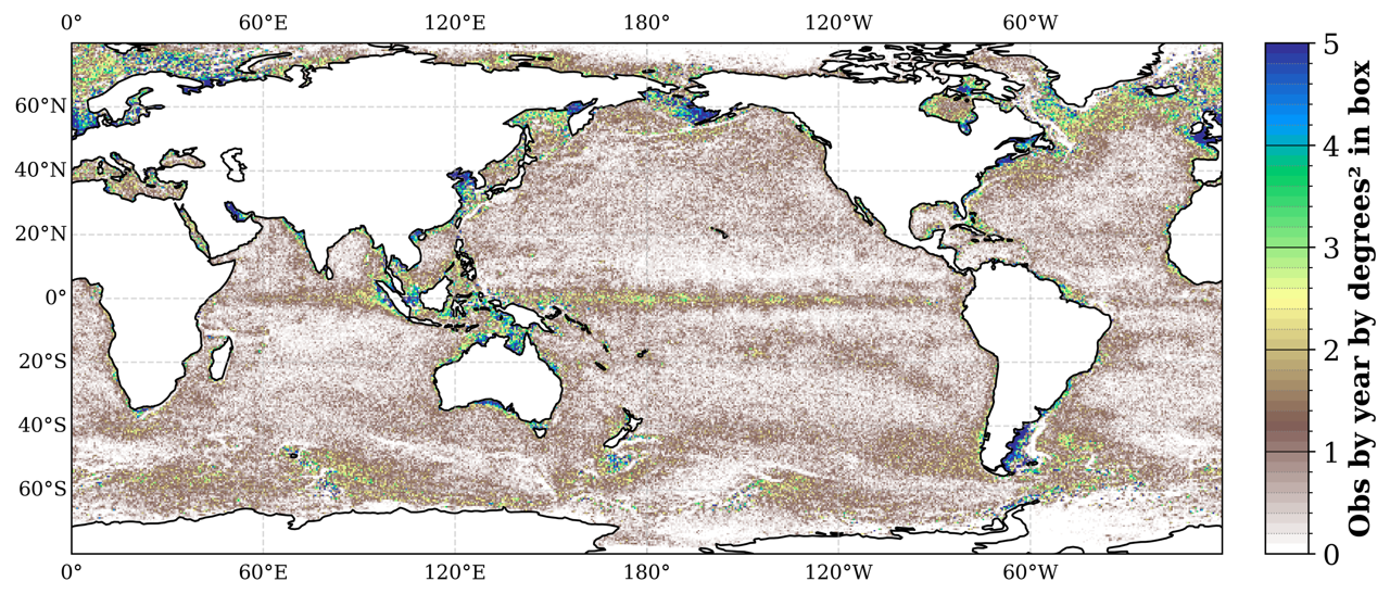
Figure 5 Frequency of lonely eddies expressed as number of observations per year and per degree².

To further document the distribution of networks, Fig. 6 presents histograms of (a) the number of observations per network and (b) the number of segments per network. These two metrics quantify the internal complexity of networks and provide insight into the range of eddy interactions captured in the dataset.

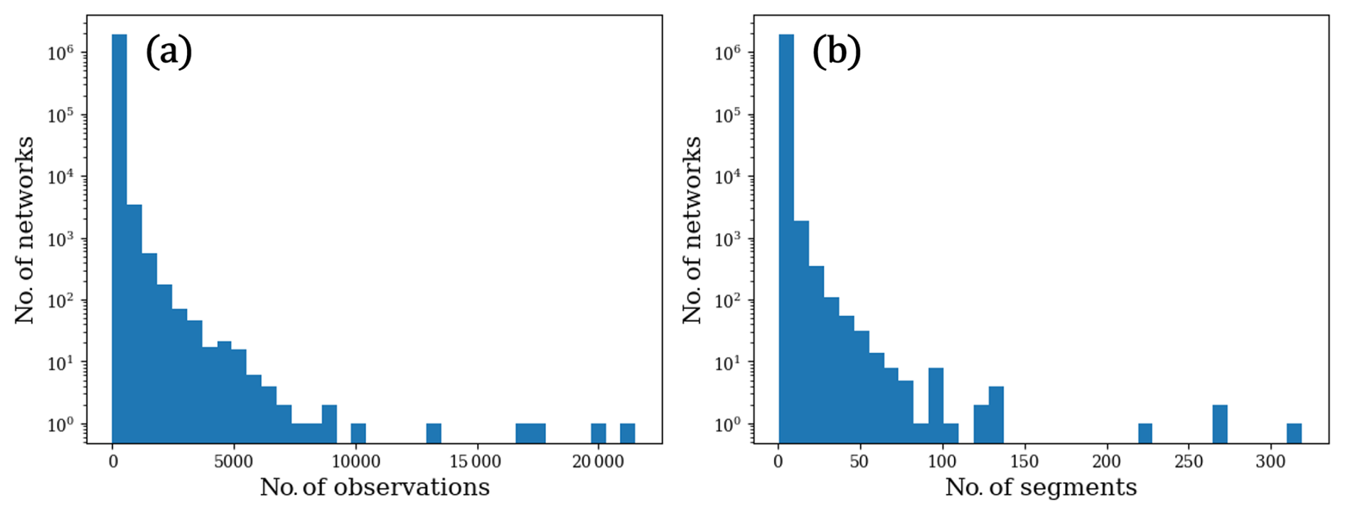
Figure 6 Histograms of META4.0 networks: (a) number of observations and (b) number of segments.

Figure 6 indicates that most networks remain relatively simple, composed of a limited number of observations and segments. Nevertheless, the dataset also contains some very large networks, as visible in Fig. 6. This wide range illustrates the strong variability of eddy life cycles and the added value of the network representation in capturing both simple, isolated structures and highly interactive, long-lived systems.

3.2.2 Comparison with the META3.2 single-trajectory dataset

In this section, the META4.0 network-based atlas is compared with the META3.2 single-trajectory dataset. It should be noted that META4.0 covers a slightly longer time period than META3.2 (approximately two additional years). However, the diagnostics presented below are expressed in relative terms or normalized frequencies, so this difference is not expected to significantly affect the interpretation of the results.

Figures 7 and 8 display frequency maps of birth and death events, respectively. In both cases, the single-trajectory dataset shows a larger number of events than the network-based approach. This difference arises because, in the single-trajectory framework, each merging or splitting tends to artificially create new births and deaths, whereas the network formalism connects these trajectories into a continuous system.

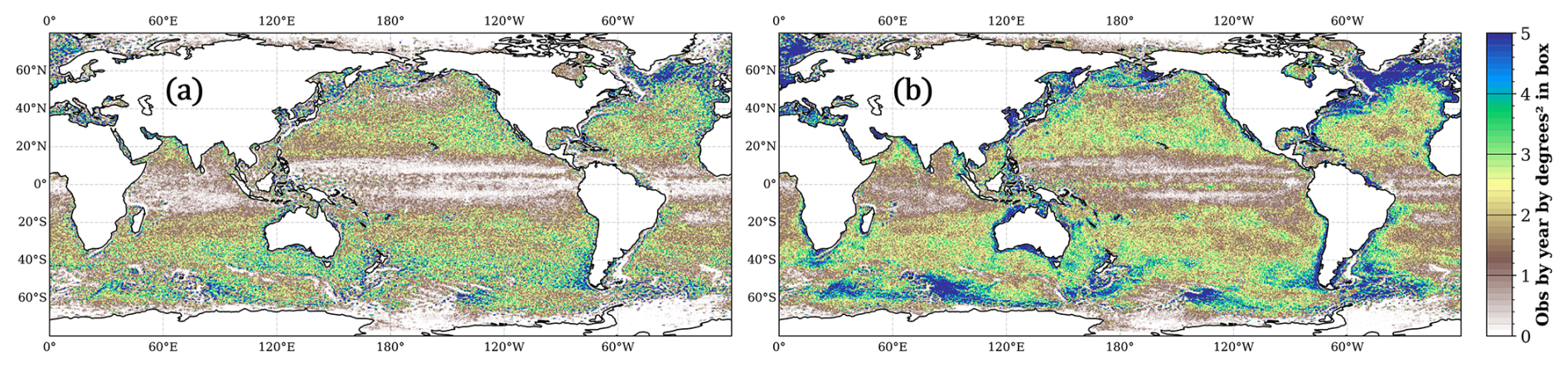
Figure 7 Comparison of birth event frequencies between (a) META4.0 networks and (b) META3.2 single trajectories.

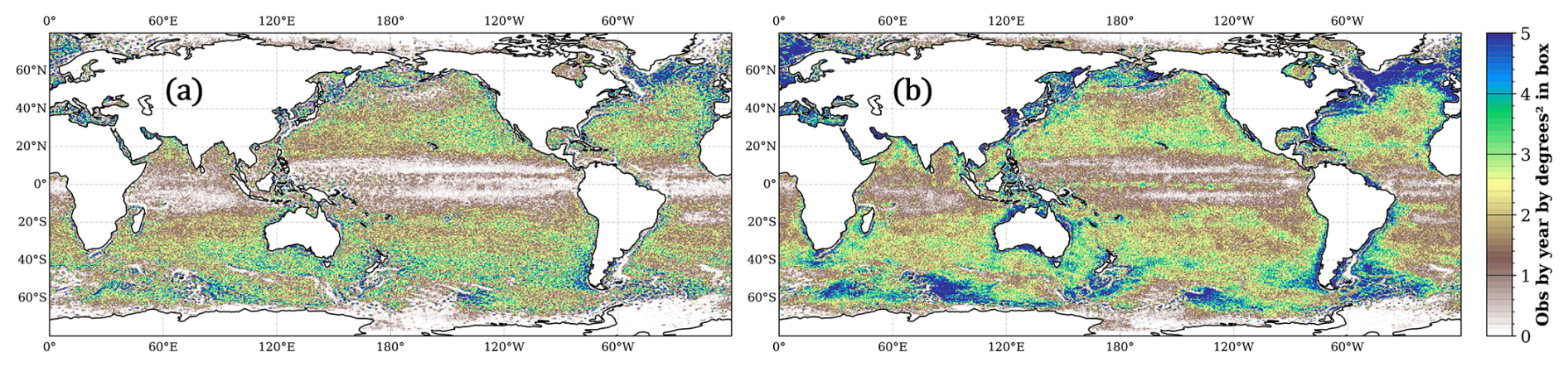
Figure 8 Comparison of death event frequencies between (a) META4.0 networks and (b) META3.2 single trajectories.

As both datasets are derived from the same set of eddy observations, this comparison highlights the main strength of the network approach: it reduces artificial discontinuities and allows for a more consistent tracking of eddy lifecycles. In practice, the META4.0 networks extend the effective lifetime of many trajectories compared with META3.2, while preserving the underlying physical signal.

To quantify these differences, we use Complementary Cumulative Distribution Functions (CCDF). The CCDF represents the fraction of eddies surviving longer than a given lifetime. This diagnostic avoids binning effects and highlights differences in the tail of the distributions. Figure 9a compares the META3.2 lifetime CCDF with the META4.0 lifetime CCDF of segments, while Fig. 9b compares META3.2 with the META4.0 CCDF of whole networks. Both comparisons show that network segments are statistically longer than single trajectories, and that networks themselves capture even longer lifetimes by connecting segments across merging and splitting events.

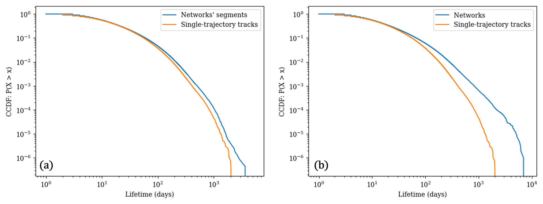
Figure 9 Comparison of lifetime CCDF between META4.0 networks' (a) segments and (b) networks and META3.2 single trajectories.

Although trajectories are divided into segments, segment lifetimes are slightly longer on average. The network framework better preserves continuity around interaction events and short detection gaps, notably through its 7 d search window.

To further illustrate these results, the spatial distribution of long-lived trajectories is also compared. Figure 10 shows the trajectories of eddies persisting longer than one year (365 d) for both datasets.

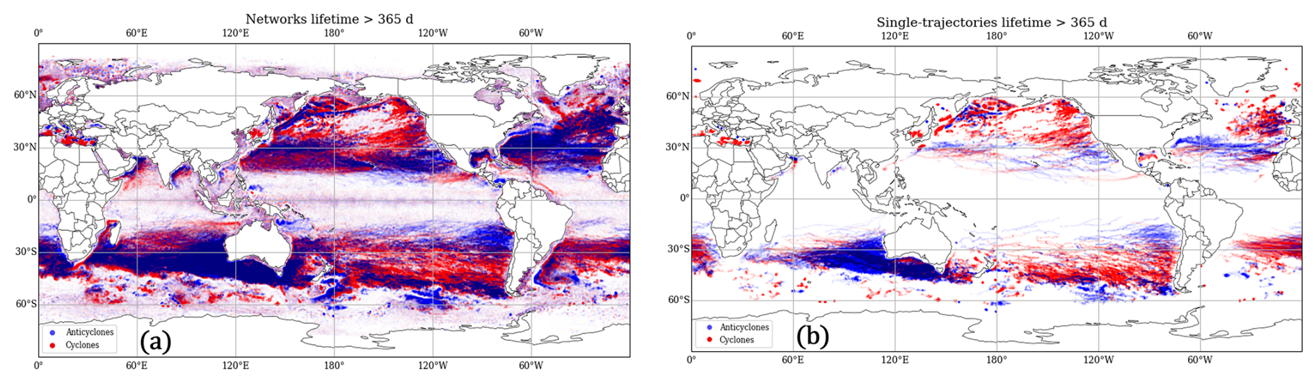
Figure 10 Comparison of eddy trajectories persisting longer than 365 d in (a) META4.0, (b) META3.2.

META4.0 detects and connects a larger number of eddies above this threshold compared with META3.2, especially in regions of intense mesoscale activity such as the western boundary currents and the Southern Ocean. This visual comparison is consistent with the idea that the network approach reduces trajectory fragmentation and improves the representation of persistent eddy structures.

Overall, these diagnostics highlight the ability of network-based tracking to represent eddy interactions and extended lifecycles beyond what can be captured using isolated trajectories.

3.3 Merging and splitting events

This section analyzes the characteristics of merging and splitting events identified with the network-based approach.

3.3.1 Spatial distribution of interaction events

Figure 11 shows frequency maps of merging and splitting events. Unlike the previous diagnostics, which are based on eddy centers, these maps are computed from the fraction of pixels covered by eddy contours involved in merging or splitting events. This representation is intended to highlight the geographical regions affected by eddy interactions and therefore accounts for the spatial extent of the eddies involved.

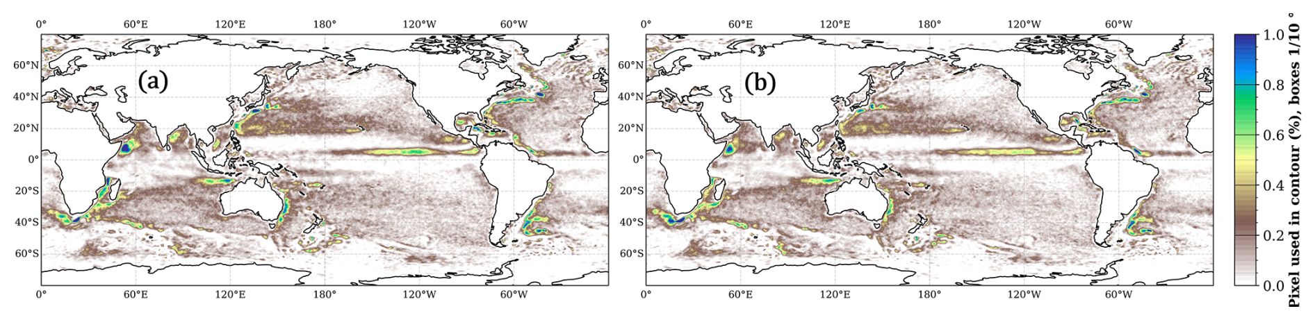
Figure 11 Frequency maps of (a) merging and (b) splitting events.

Both maps confirm that interactions are concentrated in high-energy regions, such as western boundary currents and the equatorial Pacific. The spatial signatures of merging and splitting are broadly similar, suggesting that both processes tend to occur in dynamically active areas where eddy–eddy interactions are frequent.

3.3.2 Temporal variability

Figure 12 shows the temporal evolution of the number of merging and splitting events over the 30-year record. Event counts are aggregated into successive 90 d bins to improve the readability of the long-term time series.

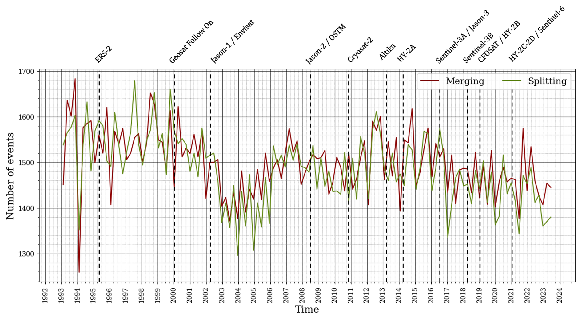
Figure 12 Temporal evolution of merging and splitting events. Temporal evolution of merging and splitting events. Vertical lines indicate the launch dates of the main satellite altimetry missions. The corresponding temporal coverage of the satellite missions and altimetric products is described in detail in Pegliasco et al. (2022).

The number of events remains relatively stable, between 1300 and 1700 per trimester, without evidence of long-term trends. Abrupt variations mainly coincide with changes in the altimeter constellation and the associated observing system, as described in Pegliasco et al. (2022).

3.3.3 Eddy properties around interaction events

To better understand how merging and splitting unfold, eddy properties are analyzed before and after interaction events. Figures 13 and 14 show the median and interquartile range of normalized effective radius and shape error in the days surrounding merging and splitting events, respectively. Eddy properties are normalized by the maximum value reached by each eddy over its lifetime before and after each merging or splitting events. This normalization allows comparison of the temporal evolution of properties within an eddy's life cycle, but does not preserve absolute size or amplitude relationships between interacting eddies. As a result, relative values before and after interactions should be interpreted as indicators of the eddy's stage within its own life cycle, rather than as direct physical comparisons between parent and resulting eddies.

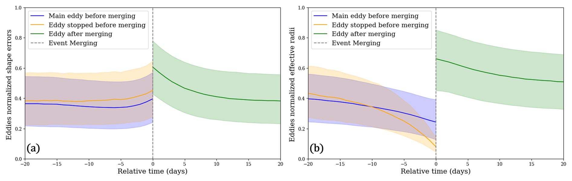
Figure 13 Median and interquartile range of eddy normalized (a) shape error and (b) effective radius around merging events.

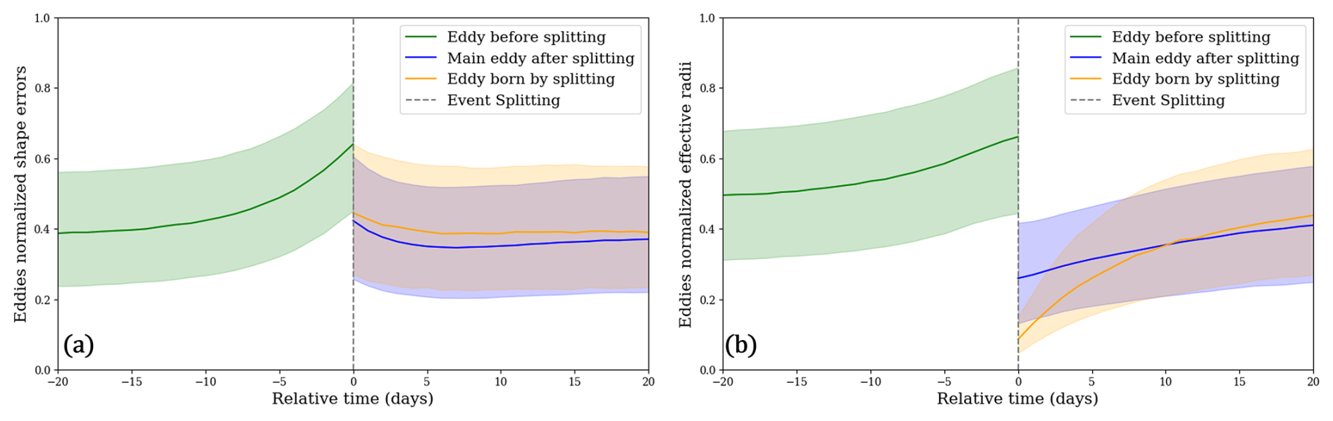
Figure 14 Median and interquartile range of eddy normalized (a) shape error and (b) effective radius around splitting events.

The results reveal systematic and consistent patterns when interpreted in a relative, life-cycle framework:

• Merging events: prior to merging, parent eddies exhibit increasing shape distortion while remaining relatively far from their maximum size within their own life cycle. Following the interaction, the resulting eddy rapidly reaches a large fraction of its lifetime maximum radius and subsequently evolves toward a more stable, less distorted configuration.

• Splitting events: eddies undergoing splitting tend to approach their maximum relative size and deformation shortly before the event. After splitting, the resulting eddies begin their evolution at relatively high normalized radii and shape errors, indicating that they inherit dynamically active structures which reorganize over the following days.

Because the diagnostics are expressed in normalized units, these figures do not quantify absolute size or amplitude transfers during interactions. The corresponding diagnostics expressed in absolute units are provided in Appendix B. They confirm that merging events are associated with larger resulting structures, whereas splitting events produce smaller daughter eddies. They confirm that merging leads to larger structures and splitting to smaller ones. The normalized analysis presented here instead highlights the timing of interaction events within the relative life cycle of eddies and their associated transient deformations.

These tendencies generalize the case-study diagnostics shown in Fig. 4, providing robust statistical evidence that merging and splitting are associated with transient structural deformation followed by a reorganization into more stable eddies.

3.3.4 Interaction events in the eddy lifecycle

To put these results into perspective, Fig. 15, inspired from Dong et al. (2012), illustrates the evolution of eddy normalized effective radius and shape errors along their normalized lifetime in the META 3.2 single-trajectory framework. This classical view highlights that eddies typically undergo an initial adjustment phase after their birth, followed by a mature stage with nearly stable properties, and finally a weakening phase characterized by decreasing radius and increasing deformation before death.

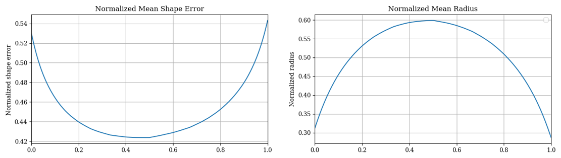
Figure 15 Evolution of normalized effective radii and deformation along normalized lifetime for the META3.2 single-trajectory framework.

The META4.0 network-based diagnostics confirm these birth–maturity–decay patterns by reproducing the statistical signatures of eddy properties around birth and death events, as shown on Figs. 16 and 17. At birth, eddies are smaller and deformed before stabilizing within weeks, while at death, they decay in size and lose coherence, consistent with Dong et al. (2012).

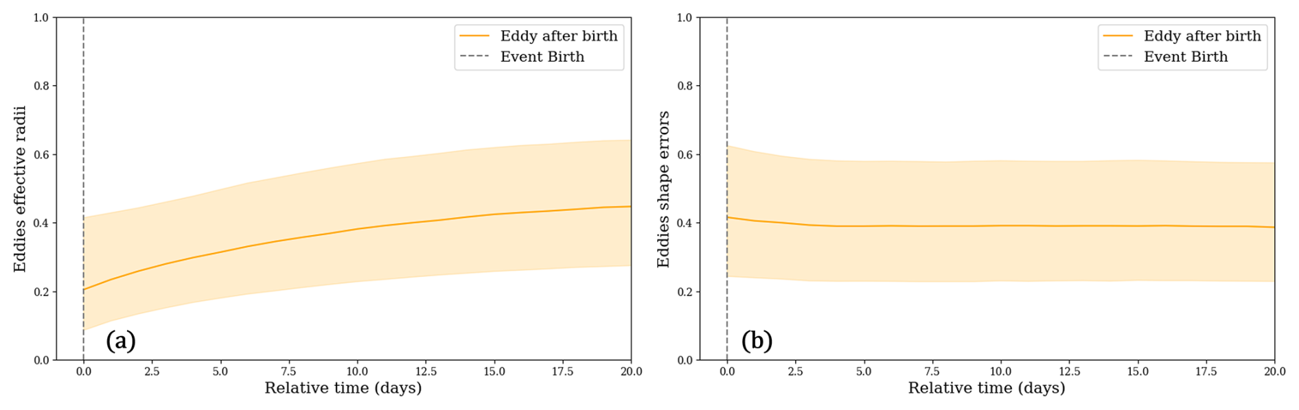
Figure 16 Evolution (median and IQR) of eddy normalized (a) shape error and (b) effective radius around birth events in META4.0.

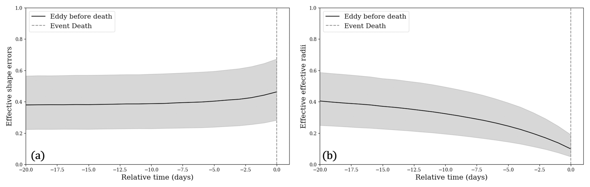
Figure 17 Evolution (median and IQR) of eddy normalized (a) shape error and (b) effective radius around death events in META4.0.

Beyond this canonical picture, however, the network framework reveals intermediate reorganizations that are absent from the single-trajectory view. The diagnostics of merging and splitting (Figs. 13 and 14) demonstrate that long-lived eddies are not only shaped by their formation and decay, but also by episodic interactions that transiently alter their structure before they restabilize.

Together, these results show that merging and splitting are frequent and robust features of mesoscale dynamics: they occur in energetic regions, at stable rates, and are systematically associated with transient deformation followed by reorganization. By embedding interaction events into the classical birth–maturity–decay framework, META4.0 provides a more complete picture of the eddy lifecycle.

3.3.5 Qualitative validation with external observations

Finally, the plausibility of some selected merging and splitting events is assessed using an independent chlorophyll concentration (CHL) product. The CLS CatSat chlorophyll fields (data courtesy of CLS) are not used to detect eddies or interaction events but provide an independent tracer field against which the altimetry eddy detections can be qualitatively compared.

Figure 18 illustrates a merging event identified from altimetry. The ADT-derived eddy contours are superimposed on both the ADT and CHL fields across four dates spanning the evolution of the event. Similarly, Fig. 19 presents a splitting event identified from altimetry and examined using the corresponding chlorophyll fields. For each case, the associated network timeline is also shown. Both examples are located off southeastern Australia (approximately 95–120° E and −40 to −30° S), a region of active mesoscale variability.

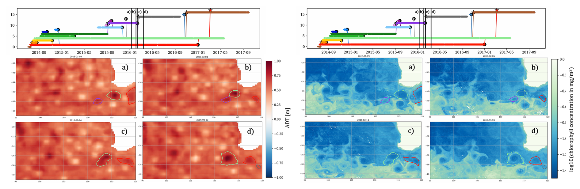
Figure 18 Merging event observed in both ADT and CHL fields (between purple and light green eddies).

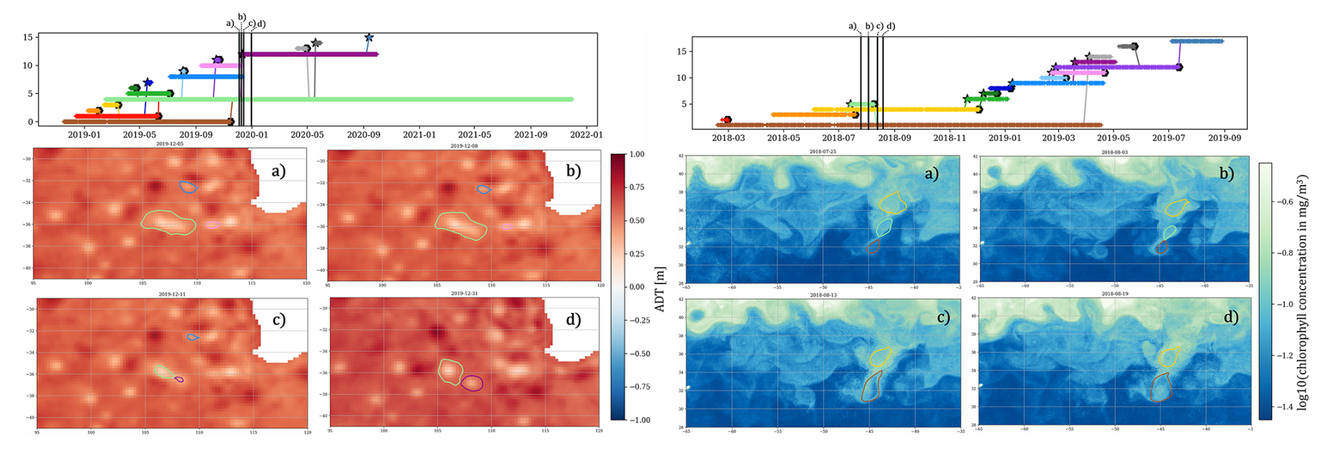
Figure 19 Splitting event observed in both ADT and CHL fields (purple and light green eddies).

The chlorophyll structures exhibit spatial patterns and temporal evolution that are consistent with the interaction events inferred from the altimetric eddy network. While CHL does not provide an independent detection of the eddy boundaries, it offers an independent tracer perspective supporting the interpretation of the detected merging and splitting events.

These examples show that the interaction events identified from altimetry are associated with coherent signatures in an independent tracer field. They should therefore be interpreted as qualitative consistency assessments rather than as independent detections of the same events. However, conducting systematic eddy detection from CHL fields at the global scale remains challenging because of cloud cover, data gaps, and uncertainties related to atmospheric corrections.

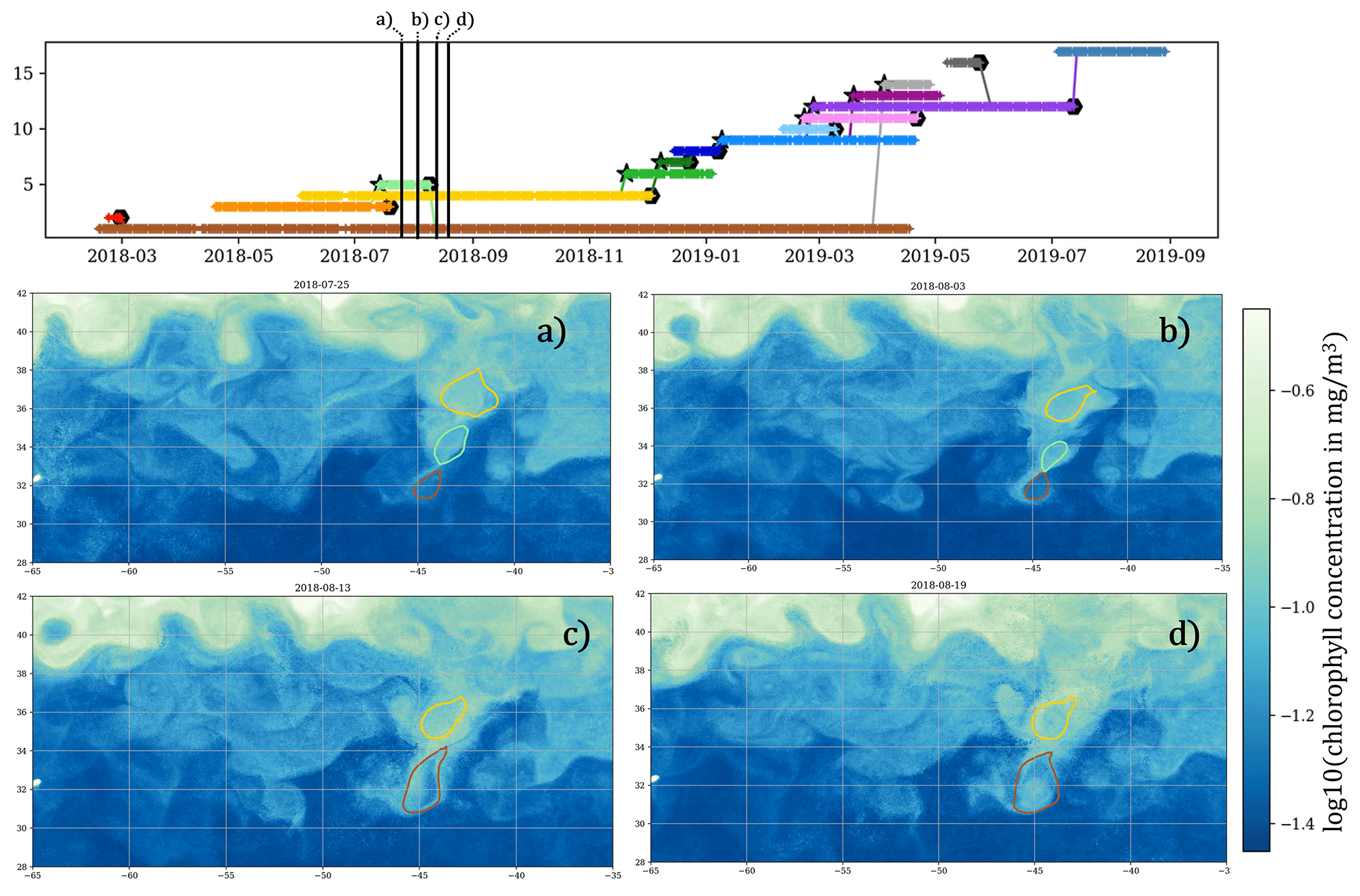
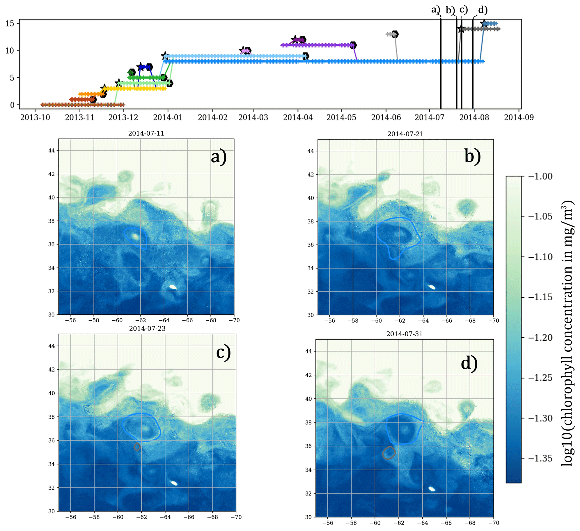
To illustrate the applicability of the approach in different dynamical environments, Appendix A presents two additional pairs of examples (one merging event and one splitting event in each region) extracted from the Agulhas and the Gulf Stream areas.

3.4 Clustering and typology of networks

This section explores whether mesoscale eddy networks can be grouped into a limited number of recurrent types based on their main properties. The objective is to identify regions of the global ocean where networks share similar structural and dynamical characteristics, thus providing a typology of mesoscale organization. This investigation is performed using a clustering analysis based on some chosen network attributes, as follows:

• The number of observations;

• The number of segments;

• The mean lifetime of segments within a network;

• The mean effective radius of eddies within a network;

• The spatial extent of networks, computed as the maximum distance between two eddies in the same network.

Different clustering algorithms and parameterizations were tested (e.g., hierarchical clustering, Gaussian Mixture Models). The k-Means algorithm (Lloyd, 1982) with five clusters was retained for its convergence speed, accuracy and robustness. For the sake of conciseness, this exploratory phase is not reported here.

Figure 20 presents the mean characteristics of the five clusters, while Fig. 21 shows the distribution of the underlying attributes. Together, these figures provide the basis for interpreting the different categories of eddy networks. The geographical distribution of the resulting classes is presented afterwards in Fig. 22.

Figure 20 Radar chart of mean attributes for the five clusters.

Figure 21 Box plots of the attributes for the five network clusters.

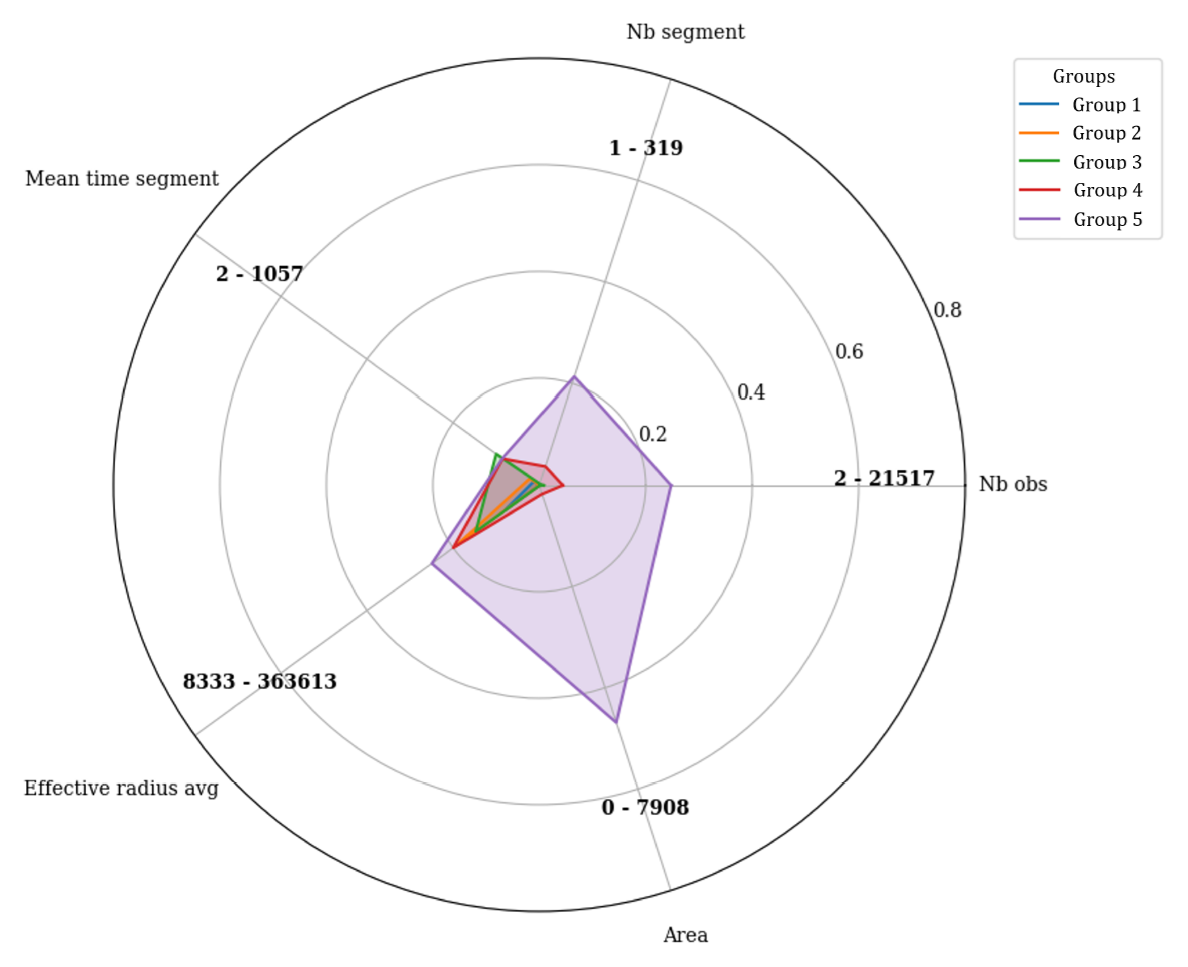
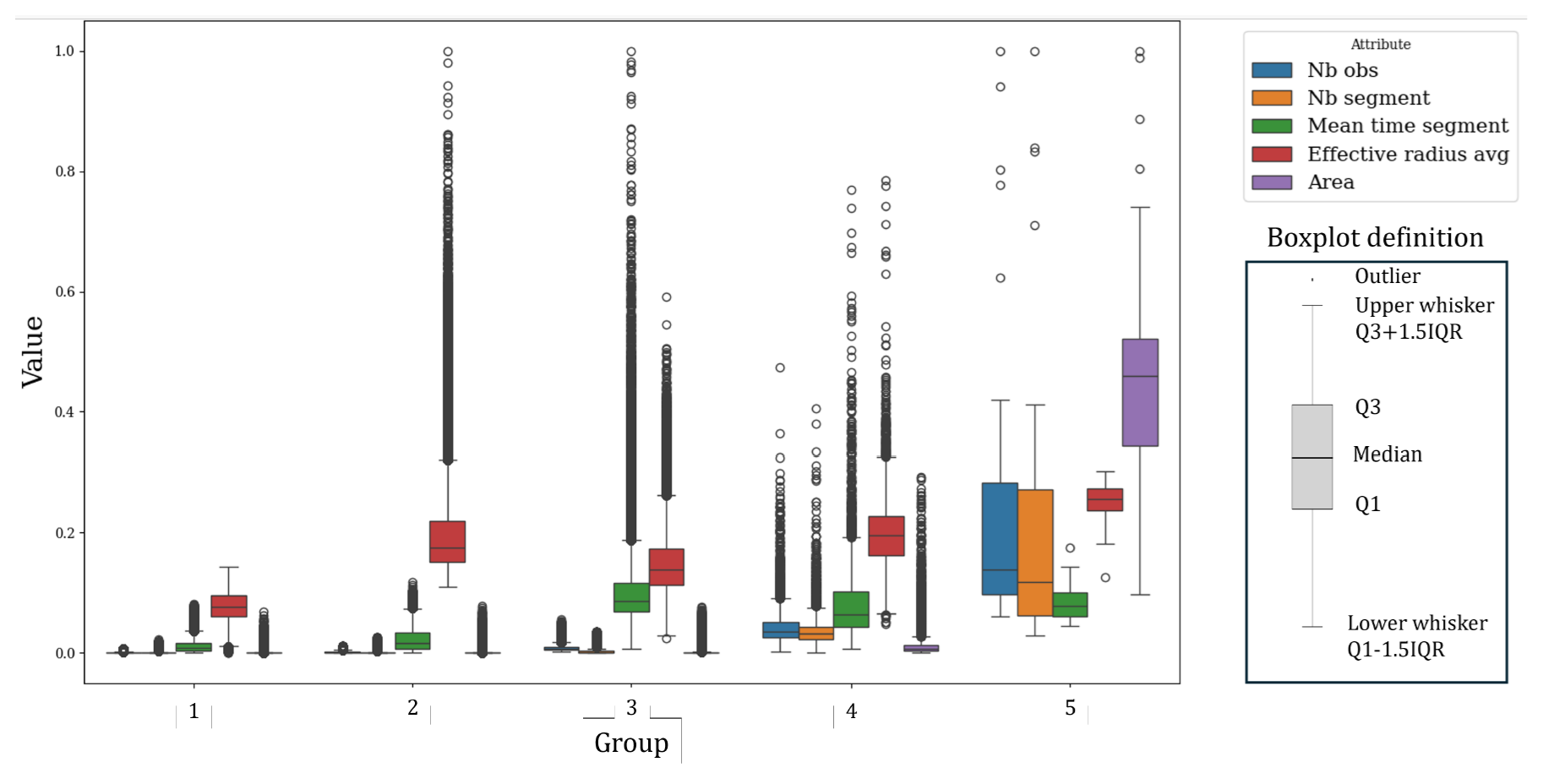
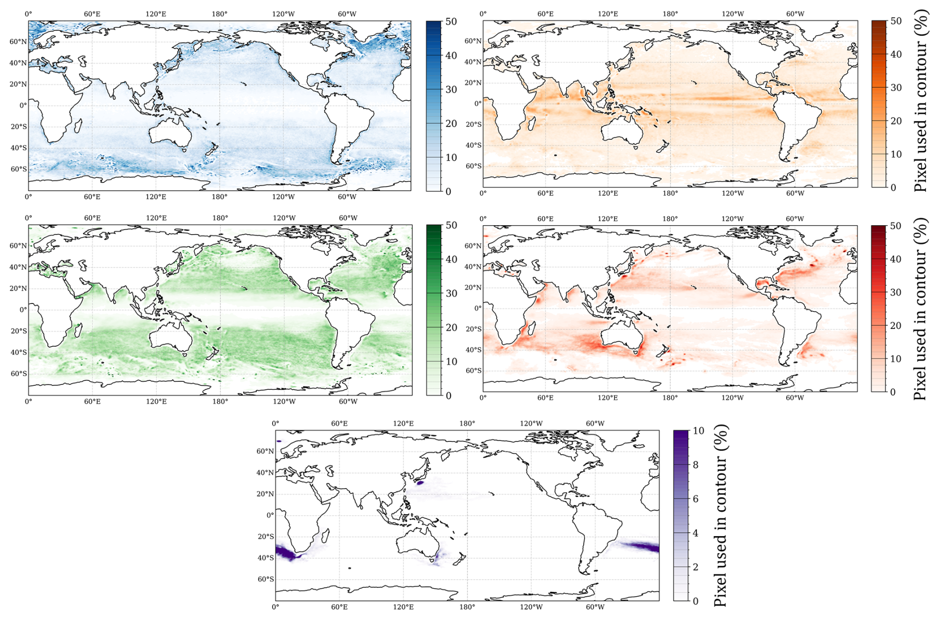
Figure 22 Spatial frequency of networks assigned to each cluster.

The five groups can be interpreted as distinct dynamical regimes of mesoscale organization:

• Group 1: Small networks of small eddies, distributed nearly everywhere. These networks likely represent the background turbulent field, with limited impact on large-scale transport.

• Group 2: Small networks of relatively large eddies, concentrated in the equatorial band. This is consistent with equatorial dynamics, where Rossby waves and instabilities generate large but weakly connected eddies.

• Group 3: Small networks of long-lived, large eddies, found in low-energy mid-latitudes. These networks reflect solitary, persistent eddies that act as local reservoirs of water masses rather than active transporters.

• Group 4: Medium-size networks of large eddies, mainly located in high-energy mid-latitude regions such as western boundary currents. These zones of strong baroclinic and barotropic instabilities foster frequent eddy interactions and exchanges.

• Group 5: The largest and longest-lived networks, concentrated in the Agulhas, the Antarctic Circumpolar Current, and other major currents (but not in the Gulf Stream which appear in the fourth group). These networks correspond to highly connected systems with strong transport capacity across ocean basins.

This typology extends the single-eddy perspective of previous atlases (e.g., META3.2) by explicitly considering the collective organization of eddies into networks. Rather than only identifying where eddies are dense, the clustering highlights where eddies evolve as isolated, long-lived structures versus where they form complex, interacting systems. From a dynamical point of view, the results distinguish between regions dominated by transient, localized structures (Groups 1–2), zones of persistent solitary eddies (Group 3), regions of intense mesoscale interactions (Group 4), and major corridors of inter-basin transport (Group 5).

Overall, the clustering highlights the heterogeneous roles of eddy networks in ocean circulation: from local stirring and storage to long-distance connectivity and redistribution of water masses.

In the next section, Lagrangian particle advection is used to complement the spatial clustering analysis by providing a dynamical assessment of water mass transport and retention within eddy networks.

3.5 Particle advection and network coherence

The coherence of eddy segments and their associated networks is assessed using Lagrangian particle advection experiments. Lagrangian approaches based on particle trajectories and Lagrangian coherent structures have been widely used to characterize eddy transport and coherence properties (e.g. Abernathey and Haller, 2018; Jones-Kellett and Follows, 2024; Tian et al., 2025).

Approaches based directly on Lagrangian coherent structures or particle trajectories characterize eddy coherence using explicitly Lagrangian criteria. In contrast, META4.0 relies on an Eulerian detection and tracking framework based on contour geometry and overlap criteria. The purpose of the particle-advection experiments presented here is therefore not to reproduce such Lagrangian tracking methodologies, but rather to assess whether the reconstructed network topology is consistent with the transport properties implied by the velocity field.

Here, virtual particles are advected using surface geostrophic velocities derived from the same altimetric sea level anomaly (ADT) product employed for eddy detection. An eddy (or eddy segment) is considered coherent when a significant fraction of the particles initially enclosed within its contour remain trapped within coherent eddy structures over time, whereas it is deemed incoherent when particles rapidly escape the eddy boundaries.

To perform this assessment, particles are uniformly initialized at a spatial resolution of $\mathrm{1}/\mathrm{50}\mathit{°}$ within the eddy speed contour at a reference date d. Particle trajectories are then integrated both forward and backward in time over a 7 d window. Particle trajectories are computed using the Lagrangian advection module of the open-source pyeddytracker package, which relies on a fourth-order Runge-Kutta (RK4) integration scheme. At d±7 d, particle positions are analyzed and assigned to the detected eddies at those dates. The coherence score is defined as the sum of the fractions of particles contained within the two eddy effective contours gathering the largest proportions of the initial particle population. This metric provides a quantitative estimate of the retentive capacity of individual segments and their associated networks, expressed as a percentage of retained particles.

Performing particle advection both forward and backward in time allows characterization of the directionality of coherence and to assess the intrinsic irreversibility of eddy interactions. Forward advection evaluates the ability of eddies to retain particles in the future, while backward advection measures the extent to which particles observed within a given eddy originate from a coherent structure in the past. Differences between forward and backward coherence therefore provide insight into the irreversible nature of eddy dynamics and particle transport.

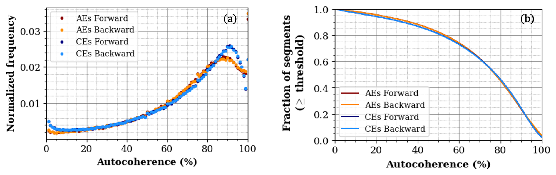
Figure 23 presents the raw and cumulative distributions of segment autocoherence scores for anticyclonic and cyclonic eddy networks. For a given segment, the resulting score is referred to as autocoherence because particle positions are compared with the future or past evolution of the same segment. In both atlases, the raw distributions exhibit a pronounced maximum at high autocoherence values (around 90 %), indicating that most detected segments behave as strongly Lagrangian coherent structures. In particular, more than 50 % of the segments display autocoherence scores exceeding 75 %, which supports the robustness of the segmentation procedure and highlights the persistence of coherent transport pathways within eddy networks.

Figure 23 (a) Raw and (b) cumulative distributions of segment autocoherence scores.

Interaction events are further evaluated using the same framework, by computing the fraction of particles that remain involved in merging or splitting processes, as opposed to escaping from interacting structures.

As described in Fig. 24, a merging event is characterized by a minor eddy M₂ merging into a dominant eddy M₁, resulting in a single eddy M that follows the trajectory of M₁, based on overlapping criteria. Conversely, a splitting event is modeled as an initial eddy S separating into a main eddy S₁, which retains the original trajectory, and a secondary eddy S₂.

Figure 25 shows the cumulative distributions of coherence scores for merging and splitting events.

Figure 24 Merging and splitting events definition.

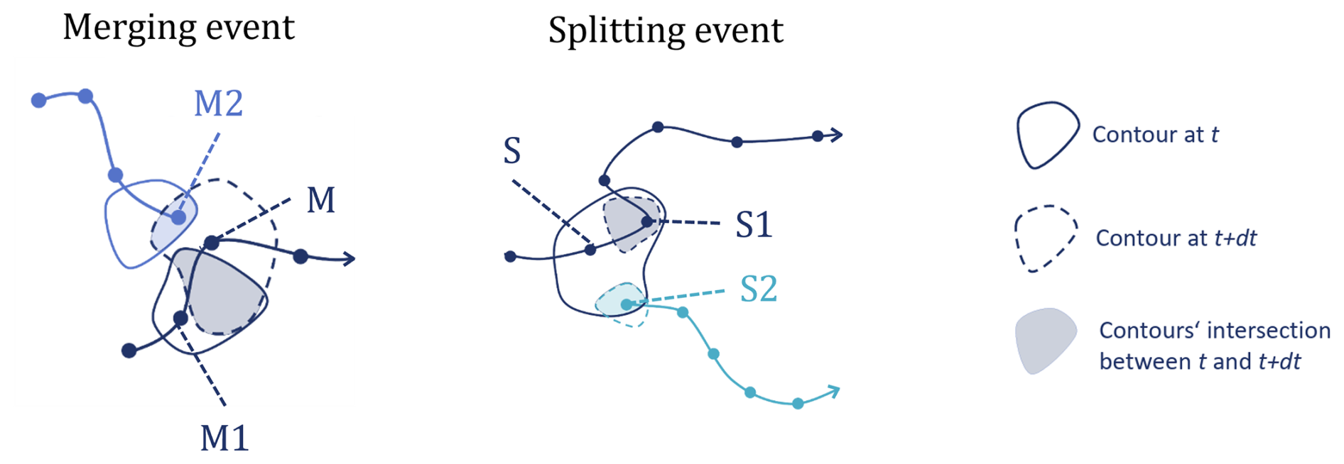
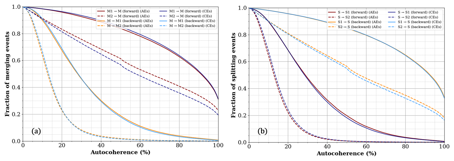
Figure 25 Cumulative distributions of coherence scores for (a) merging and (b) splitting events.

Forward advection reveals a strong coherence of merging processes, as particles initially enclosed within interacting eddies remain largely confined within the merged structure. In contrast, backward advection exhibits significantly lower coherence, reflecting the irreversible mixing of particle trajectories once the eddies have merged. More than 60 % of detected merging events display forward coherence scores above 80 % for the dominant eddy M₁, whereas the secondary eddy M₂ generally exhibits lower coherence, with only about 40 % exceeding the same threshold. This asymmetry likely reflects the weaker dynamical integrity of M₂, which is typically smaller and more rapidly distorted during the merging process.

Conversely, Fig. 25b shows that splitting events display higher backward autocoherence. Backward integration highlights the convergence of particle trajectories toward a single coherent structure in the past, while forward advection results in a dispersion of particles among multiple offspring eddies. More than 60 % of detected splitting events exhibit backward coherence scores above 80 % for the main eddy S₁. The secondary eddy S₂ shows systematically lower coherence, with only about 35 % of events exceeding this threshold, consistent with its more recent formation and reduced ability to retain particles.

Overall, these diagnostics show that most detected interaction events are associated with coherent Lagrangian transport patterns that are consistent with the reconstructed network structure.

It should be noted, however, that the velocity fields used for particle advection are derived from the same altimetric product as that employed for eddy detection. As a result, the coherence assessment is not fully independent of the detection methodology, unlike diagnostics based on external tracers such as chlorophyll or sea surface temperature. Nevertheless, the particle-based analysis evaluates a different aspect of the dataset. While the detection and tracking procedures are based on Eulerian contour geometry, the advection experiments assess the Lagrangian transport properties implied by the same velocity field. The analysis therefore provides a consistency check of the reconstructed networks rather than an independent validation of the underlying eddy detections.

Additional limitations include the finite 7 d advection window, which may miss shorter-lived interactions or intermediate events occurring within this period. Despite these limitations, the consistency of the results across multiple diagnostics supports the robustness of the proposed framework.

Finally, tools to perform Lagrangian particle advection analyses on individual eddy networks are provided within the pyeddytracker toolbox (https://py-eddy-tracker.readthedocs.io/en/v3.6.1/python_module/16_network/ pet_follow_particle.html#sphx-glr-python-module-16-network-pet-follow-particle-py, last access: 23 September 2026). These tools allow, for instance, the advection of particles within a given network, the visualization of their trajectories, and the analysis of interaction events along their temporal evolution.

4 Code and data availability

The detection, tracking and networking algorithms have been freely released under a GPL V3 license (https://doi.org/10.5281/zenodo.6333989, Delepoulle et al., 2022) in the Python language.

The META4.0 delayed-time (DT) dataset is available in an AVISO repository at https://doi.org/10.24400/527896/a01-2026.001 (CLS and CNES, 2026). An associated handbook describes the atlas as well as the variables stored in the NetCDF files and gives an insight into data manipulation. A large gallery of illustrated and documented routines to help with the data manipulation and visualization is also available, and is updated when new methods are developed (https://py-eddy-tracker.readthedocs.io/en/v3.3.1/, last access: 23 September 2026) (pyeddytracker, 2022).

5 Conclusions

In this article, the new global Mesoscale Eddy Trajectory Atlas META4.0 has been introduced. The dataset was computed using the pyeddytracker framework, developed in Python, and the routines for data manipulation and visualization have been fully documented and made publicly available.

The main novelty of META4.0 lies in the introduction of eddy networks as a new framework for eddy tracking. Unlike the previous single-trajectory strategy, the network-based approach enables the identification of merging and splitting events and organizes trajectories into segments belonging to larger interacting structures. In this way, networks group together all eddies linked through interaction events. This representation adds a new layer of complexity to eddy tracking and allows for a more realistic description of eddy life cycles, explicitly accounting for their interactions and temporal connectivity.

A series of exploratory diagnostics was conducted to assess the robustness and relevance of the dataset. Global statistics and a comparison with the META3.2 single-trajectory atlas demonstrated that the network approach extends eddy lifetimes and refines the reconstruction of their pathways. Merging and splitting events were characterized in terms of their spatial distribution, temporal variability, and impact on eddy properties throughout their life cycles. These analyses revealed that interaction events play a fundamental role in shaping eddy evolution, a dimension that cannot be captured within a single-trajectory framework. Indeed, the results highlight that merging and splitting are frequent and robust features of mesoscale dynamics that occur in energetic regions, at stable rates, and are systematically associated with transient deformation followed by reorganization. A qualitative validation using independent chlorophyll concentration data further confirmed the realism of the detected interactions for selected case studies. By adding interaction events into the classical birth–maturity–decay framework, META4.0 provides a more complete picture of the eddy lifecycle.

Beyond individual events, the network representation provides a natural framework to investigate the collective organization of mesoscale eddies. A clustering analysis identified five distinct typologies of eddy networks, revealing contrasted regimes of ocean circulation ranging from localized, short-lived structures to highly connected systems associated with major current regions. These results highlight the emergence of large-scale connectivity patterns resulting from repeated eddy interactions.

Altogether, the results demonstrate that network-based tracking constitutes a significant advance in the description of mesoscale dynamics. By extending the representation beyond isolated trajectories, META4.0 enables a more comprehensive reconstruction of eddy origins, pathways, interactions, and cross-basin connectivity. The Lagrangian diagnostics further demonstrate that eddy interactions are intrinsically irreversible processes, with distinct signatures in forward and backward particle transport. Beyond this dynamical interpretation, the consistency of these signatures with the expected behavior of merging and splitting events provides a coherent validation of the detected interactions and of the network-based representation. Although the advection relies on the same velocity fields as those used for eddy detection, these results offer a physically meaningful assessment of the realism of the reconstructed networks.

Nevertheless, some limitations of the present framework should be acknowledged. The reconstruction of eddy networks relies on Eulerian geometric criteria based on contour overlap and temporal continuity, combined with empirically selected tracking parameters. Consequently, the identified merging and splitting events should not be interpreted as a unique or exhaustive representation of all physical eddy interaction processes. While the Lagrangian diagnostics provide additional evidence for the physical consistency of the reconstructed networks, they are performed a posteriori and do not constitute an independent tracking framework.

Future developments will include the application of the detection and tracking methods to next-generation sea surface height products, including datasets benefiting from the SWOT mission and forthcoming high-resolution altimetric products. In parallel, colocations with temperature and salinity Argo float profiles will allow the reconstruction of the three-dimensional structure of eddies, extending previous efforts that combine altimetry with in situ observations to better characterize mesoscale dynamics. These complementary observations will enrich the current datasets and enable a more complete characterization of eddy dynamical and biogeochemical impacts.

Particular attention will be devoted to the development of quantitative validation approaches for merging and splitting events based on independent observations, including biogeochemical tracers and in situ measurements. Such analyses will help confirm the physical realism of reconstructed eddy interactions and further improve the characterization of mesoscale connectivity. Complementary transport-based and Lagrangian diagnostics will also be investigated as additional tools to evaluate the consistency of reconstructed eddy interactions and to compare alternative representations of eddy connectivity.

Appendix A: Additional surface chlorophyll concentration qualitative validation examples

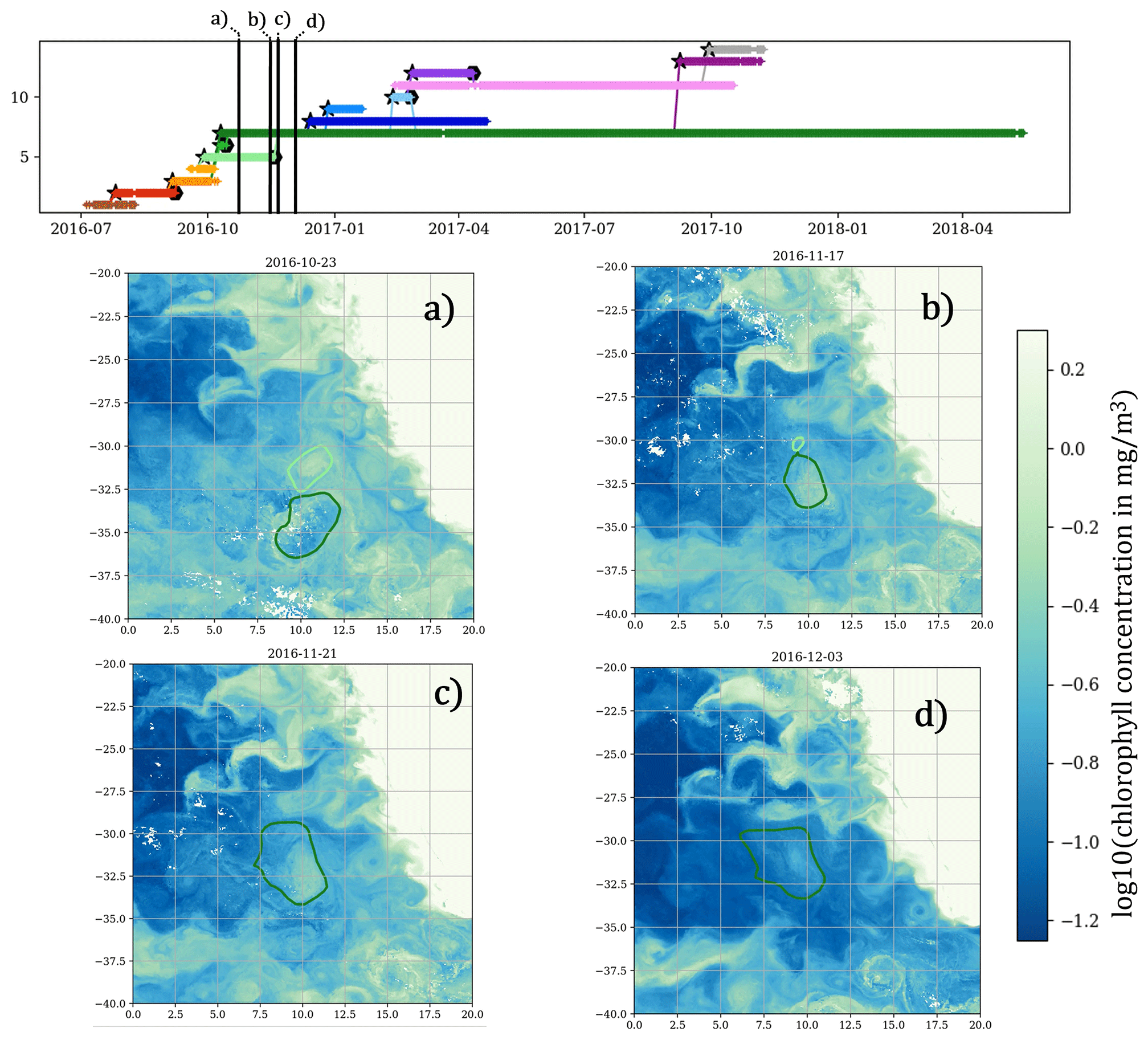
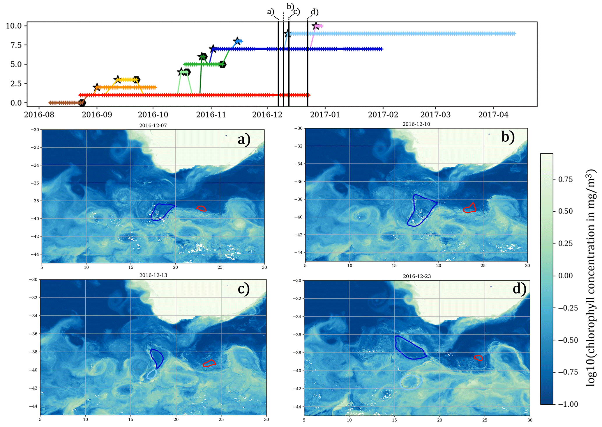
To complement the examples presented in Sect. 3.3.5, additional merging and splitting events are shown in two other dynamically active regions: the Agulhas and the Gulf Stream zones. As in the main text, ADT-derived eddy contours are superimposed on surface chlorophyll concentration fields.

Figures A1 and A2 present one merging event and one splitting event observed in the Agulhas region. Figures A3 and A4 show equivalent examples in the Gulf Stream system. In all cases, the chlorophyll fields exhibit coherent structures whose evolution is qualitatively consistent with the interaction events inferred from the altimetric network.

These figures are not intended to provide an exhaustive validation of merging and splitting detections. However, they offer additional qualitative evidence that the interaction events reconstructed from altimetric observations are associated with identifiable tracer structures across multiple regions of the global ocean.

Figure A1 Additional examples of a merging event in the Agulhas zone.

Figure A2 Additional examples of a splitting event in the Agulhas zone.

Figure A3 Additional examples of a merging event in the Gulf Stream zone.

Figure A4 Additional examples of a splitting event in the Gulf Stream zone.

Appendix B: Absolute evolution of eddy properties during interaction events

For completeness, Figs. B1 and B2 present the same diagnostics as Figs. 13 and 14, but using absolute values rather than normalized quantities.

While the normalization adopted in the main text facilitates comparison between eddies of different sizes and amplitudes, the absolute diagnostics provide the physical magnitude of the variations associated with interaction events. The results are consistent with the conclusions drawn from the normalized analysis: merging events generally produce larger eddies, whereas splitting events result in smaller offspring structures. The increase in shape error before interactions and the subsequent relaxation toward more stable configurations are also visible in absolute units.

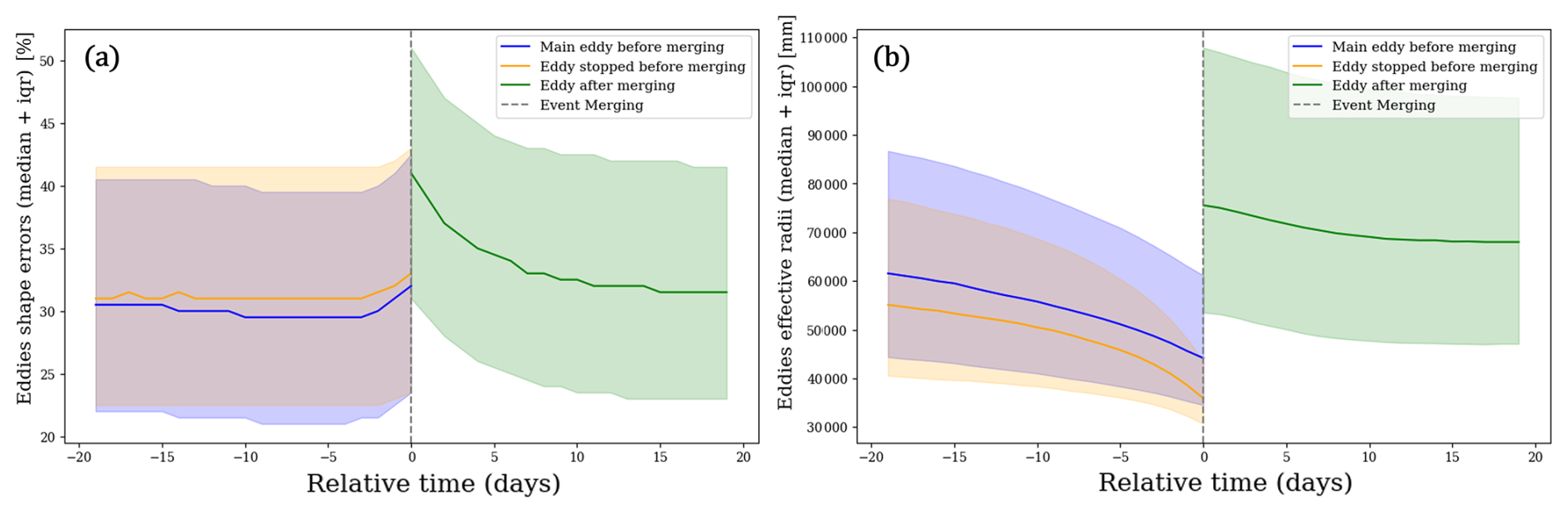
Figure B1 Median and interquartile range of eddy absolute (a) shape error and (b) effective radius around merging events.

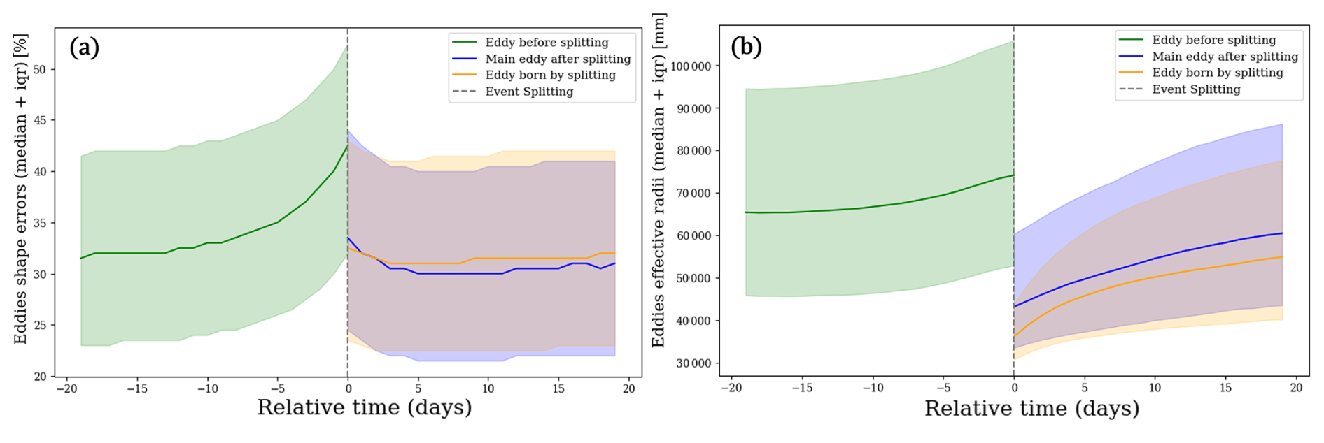
Figure B2 Median and interquartile range of eddy absolute (a) shape error and (b) effective radius around splitting events.