SPAMS10: an InSAR-derived soil motion parameter dataset to model relative peat surface elevation changes

Peat subsidence poses a significant challenge to long-term land and environmental stability by increasing flood risk and producing greenhouse gas emissions. Field monitoring with extensometers reveals variability in relative surface elevation changes, which are then modeled using simple parameterization for the motion of soils (SPAMS). To extend the spatial scale of monitoring, Interferometric Synthetic Aperture Radar (InSAR) time series are used. InSAR-derived SPAMS parameters provide displacement models that can describe peat subsidence and dynamics with a set of parameters, namely four parameters for modeling and six variance-covariance terms for model uncertainties. We publish the SPAMS10 dataset, which refers to the descriptive displacement model SPAMS with ten parameters. The dataset also provides additional contextual information, such as soil code, at the parcel level, defined by the administrative boundary of an agricultural field. This dataset promotes data sharing among stakeholders, shifting products from InSAR-based relative elevation estimates to InSAR-derived displacement model parameters. These parameters enable the reconstruction of displacement models for peat subsidence analyses. The dataset is available through the 4TU.ResearchData repository: https://doi.org/10.4121/dfbe9109-d058-4a64-a5b4-1cc9d9a5f836 (Lumban-Gaol et al., 2025) and is distributed under a Creative Commons Attribution 4.0 International (CC BY 4.0) license.

1 Introduction

Land subsidence, defined as the gradual downward displacement of the Earth's surface across extensive geographical regions relative to a designated reference level, represents a critical geophysical process with significant environmental implications. In peatland areas, anthropogenic activities such as lowering the water table for agricultural purposes and urban development have led to peat subsidence, a phenomenon often considered a “silent hazard” due to its slow progress but with severe environmental and socioeconomic consequences (Erkens et al., 2016; Page et al., 2020; Herrera-García et al., 2021). This phenomenon contributes to numerous environmental challenges, including increased CO₂ emissions (Wösten et al., 1997; Page et al., 2011; Hooijer et al., 2012), flood risk (Dixon et al., 2006; Ikkala et al., 2021), infrastructure damage (Gambolati et al., 2006), and reduced land productivity (Brouns et al., 2015; Hein et al., 2022). Effective mitigation strategies require comprehensive monitoring systems to assess spatial and temporal impacts of the subsidence, supported by robust and scalable models of surface elevation changes.

Peat subsidence occurs mainly due to oxidation and compaction processes (Schothorst, 1977; Hoogland et al., 2012; Hooijer et al., 2012; van Asselen et al., 2018). Oxidation involves the decomposition of organic matter in aerated zones when exposed to oxygen, causing CO₂ emissions and volume reduction (Gambolati et al., 2005, 2006; van Huissteden et al., 2006; van Asselen et al., 2009). Compaction refers to the compression of soil under vertical effective stress from overburden weight and the reduced pore pressure resulting from oxidation (Stephens et al., 1984; van Asselen et al., 2009; Hooijer et al., 2012).

Efforts in monitoring peat subsidence have been continuously made using ground-based and remote sensing techniques, including leveling (Pleijter and van den Akker, 2007), extensometers (van Asselen et al., 2020; Burbey, 2020), peat cameras (Evans et al., 2021), and interferometric synthetic aperture radar (InSAR) (Conroy et al., 2024). Modeling efforts incorporate these observations and peat subsidence processes, utilizing peat thickness and surface water levels to approximate the aerated zone thickness in order to estimate the subsidence rates (Hoogland et al., 2012), relating drainage depth and soil temperature to subsidence (Stephens et al., 1984; Zanello et al., 2011), and applying meteorological data to model soil surface motion (Conroy et al., 2023a).

Despite these advances, the estimation of the elevation of peat soils from geodetic observations is still cumbersome. This is due to its high spatio-temporal variability, its sensitivity to land use, and the lack of well-identifiable benchmarks. Moreover, in the case of InSAR one also needs to resolve integer phase ambiguities (Hanssen, 2001) and deal with loss-of-lock events, in which the connection between subsequent data acquisition is lost (Conroy et al., 2023b). To address this, we propose SPAMS10, a dataset derived from InSAR observations and intended for the study of peatland surface dynamics. SPAMS10 refers to the descriptive displacement model: SPAMS (a Simple Parameterization for the Motion of Soils) and the number of parameters: ten. The dataset can be expressed as

$$\begin{array}{}\text{(1)}& {\displaystyle }{\displaystyle }\widehat{\underset{\mathrm{¯}}{x}}=\left[\begin{array}{c}{\widehat{\underset{\mathrm{¯}}{x}}}_{\mathrm{P}}\\ {\widehat{\underset{\mathrm{¯}}{x}}}_{\mathrm{E}}\\ {\widehat{\underset{\mathrm{¯}}{x}}}_{\mathrm{I}}\\ \mathit{\tau }\end{array}\right],\text{vech}\left({\mathbf{Q}}_{\widehat{x}}\right)=\left[\begin{array}{c}{\mathit{\sigma }}_{{\widehat{x}}_{\mathrm{P}}}^{\mathrm{2}}\\ {\mathit{\sigma }}_{{\widehat{x}}_{\mathrm{P}}{\widehat{x}}_{\mathrm{E}}}\\ {\mathit{\sigma }}_{{\widehat{x}}_{\mathrm{P}}{\widehat{x}}_{\mathrm{I}}}\\ {\mathit{\sigma }}_{{\widehat{x}}_{\mathrm{E}}}^{\mathrm{2}}\\ {\mathit{\sigma }}_{{\widehat{x}}_{\mathrm{E}}{\widehat{x}}_{\mathrm{I}}}\\ {\mathit{\sigma }}_{{\widehat{x}}_{\mathrm{I}}}^{\mathrm{2}}\end{array}\right],\end{array}$$

which includes the four SPAMS soil motion parameters $\widehat{\underset{\mathrm{¯}}{x}}$: the scaling factor of precipitation ${\widehat{\underset{\mathrm{¯}}{x}}}_{\mathrm{P}}$, the scaling factor for evapotranspiration ${\widehat{\underset{\mathrm{¯}}{x}}}_{\mathrm{E}}$, the irreversible subsidence rate ${\widehat{\underset{\mathrm{¯}}{x}}}_{\mathrm{I}}$ in mm d⁻¹, and the integration time τ in days. The underline indicates the stochastic nature of the estimate. The integration time τ is estimated and has a rather constant value, with a mean of 69 d and a standard deviation of two days. For convenience, we treat this parameter as deterministic and do not include it in the stochastic model. Focusing only on the first three parameters, we use the six statistical variance and covariance terms $\text{vech}\left({\mathbf{Q}}_{\widehat{x}}\right)$ of the first three parameters for each parcel.

The parameters $\widehat{x}$ and the half-vectorized covariance matrix, $\text{vech}\left({\mathbf{Q}}_{\widehat{x}}\right)$, define the SPAMS10 dataset. These components serve as inputs for the SPAMS model (Conroy et al., 2023a) to simulate relative elevation changes, enabling the modeling of both reversible and irreversible surface elevation changes and the quantification of the associated uncertainties. They also enable the forecasting of past and future subsidence under the assumption that conditions such as soil stratigraphy, groundwater management, and land use remain constant over time.

We focus on regions particularly vulnerable due to extensive agricultural use and underlying soft soils. Realizations of relative surface elevation based on SPAMS10 estimates of irreversible annual subsidence rates are critical for purposes such as assessing gas emissions and flood risk. The SPAMS10 parameters are intended as a first approximation and will be updated as the displacement model and geophysical understanding of the study area evolve.

2 Methods

The SPAMS10 dataset is derived from a multi-stage methodology that uses InSAR observations with SPAMS as the displacement model. Figure 1 shows the five main stages in creating the dataset: (i) input data, (ii) point scatterers (PS) and distributed scatterers (DS) analysis to obtain the observed phases, (iii) contextual grouping and coherent segment identification, (iv) SPAMS model parameter estimation, and (v) the SPAMS10 dataset. This study uses Sentinel-1A/B satellite acquisitions with the interferometric wide swath mode and a single VV polarization. Four satellite tracks, two ascending (088 and 161) and two descending (37 and 110), illuminate the area of interest, which is the Krimpenerwaard region in the Netherlands. We use data from 2015 to 2026, with a total number of acquisition of 477, 488, 484, and 493, respectively. All single look complex (SLC) images are preprocessed using Doris (Kampes and Usai, 1999; Kampes et al., 2004; Arikan et al., 2008) for coregistration.

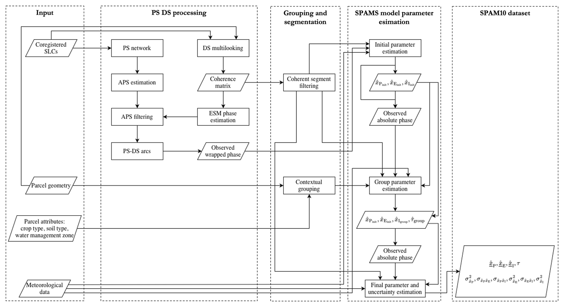
Figure 1 A schematic workflow to create the dataset. We divide the processes into five general stages: (i) input data, (ii) PS and DS analysis to obtain the observed phases, (iii) contextual grouping and coherent segment identification, (iv) SPAMS model parameter estimation, and (v) the SPAMS10 dataset.

The resulting coregistered SLC stack undergoes two separate analyses, for DS and PS. During DS analysis, the SLC images are multilooked over a window of Ω pixels within the known parcel geometry to estimate the full complex coherence matrix $\widehat{\mathrm{\Gamma }}$. This matrix describes the degree of similarity between pairs of SAR images for all possible combinations of N SAR acquisitions, per parcel. It is used as a metric for the precision of the interferometric phase. The matrix is defined as

$$\begin{array}{}\text{(2)}& {\displaystyle }{\displaystyle }\widehat{\mathrm{\Gamma }}=\left[\begin{array}{cccc}{\widehat{\mathit{\gamma }}}_{\mathrm{11}}& {\widehat{\mathit{\gamma }}}_{\mathrm{12}}& \mathrm{\cdots }& {\widehat{\mathit{\gamma }}}_{\mathrm{1}N}\\ {\widehat{\mathit{\gamma }}}_{\mathrm{21}}& {\widehat{\mathit{\gamma }}}_{\mathrm{22}}& \mathrm{\cdots }& {\widehat{\mathit{\gamma }}}_{\mathrm{2}N}\\ \mathrm{⋮}& \mathrm{⋮}& \mathrm{\ddots }& \mathrm{⋮}\\ {\widehat{\mathit{\gamma }}}_{N\mathrm{1}}& {\widehat{\mathit{\gamma }}}_{N\mathrm{2}}& \mathrm{\cdots }& {\widehat{\mathit{\gamma }}}_{NN}\end{array}\right],\end{array}$$

where $\widehat{\mathit{\gamma }}$ is the complex coherence estimator, expressed as Hanssen (2001)

$$\begin{array}{}\text{(3)}& {\displaystyle }{\displaystyle }{\widehat{\mathit{\gamma }}}_{ij}={\displaystyle \frac{{\sum }_{n\in \mathrm{\Omega }}{y}_i^{\left(n\right)}{y_j^{*}}^{\left(n\right)}}{\sqrt{\left({\sum }_{n\in \mathrm{\Omega }}{\left|y_i^{\left(n\right)}\right|}^{\mathrm{2}}\right)\left({\sum }_{n\in \mathrm{\Omega }}{\left|y_j^{\left(n\right)}\right|}^{\mathrm{2}}\right)}}},\end{array}$$

where $y_i^{\left(n\right)}$ and $y_j^{\left(n\right)}$ are the complex values of pixel n in image i and j. Pixel n is within the window Ω, and $(\cdot {)}^{*}$ denotes the complex conjugate. Based on the estimate of the full complex coherence matrix we estimate a single set of DS phases, equivalent to those obtained from interferometric combinations with one reference image. We refer to this as the equivalent single mother phase ${\widehat{\mathit{\varphi }}}_{\text{ESM}}$. By applying the eigendecomposition-based maximum likelihood estimator of interferometric phase (Ansari et al., 2018) to the full coherence matrix, the complete set of interferometric combinations is reduced to a single set of phases. Assuming unbiased estimation, the phase variance follows the Cramer–Rao bound ${\mathit{\sigma }}_{{\widehat{\mathit{\varphi }}}_{ij,\text{CRB}}}^{\mathrm{2}}$, which is expressed as Hanssen (2001)

$$\begin{array}{}\text{(4)}& {\displaystyle }{\displaystyle }{\mathit{\sigma }}_{{\widehat{\mathit{\varphi }}}_{ij,\text{CRB}}}^{\mathrm{2}}={\displaystyle \frac{\mathrm{1}-|{\mathit{\gamma }}_{ij}{|}^{\mathrm{2}}}{\mathrm{2}L|{\mathit{\gamma }}_{ij}{|}^{\mathrm{2}}}},\end{array}$$

where L is the effective number of looks, which is the ratio between the number of pixels Ω within an estimate window and the oversampling ratio (Hanssen, 2001). Based on these procedures, we obtain a phase time series per parcel denoted as

$$\begin{array}{}\text{(5)}& {\displaystyle }{\displaystyle }{\widehat{\mathit{\varphi }}}_{\text{ESM}}={\left[\begin{array}{cccc}{\widehat{\mathit{\varphi }}}_{\mathrm{11}}& {\widehat{\mathit{\varphi }}}_{\mathrm{12}}& \mathrm{\cdots }& {\widehat{\mathit{\varphi }}}_{\mathrm{1}N}\end{array}\right]}^{\mathrm{T}}.\end{array}$$

From the same coregistered SLC stack, the atmospheric phase screen (APS) is estimated using a PS network, following the DePSI framework (van Leijen, 2014). To perform APS filtering, we first need to disentangle the atmospheric signal from other phase contributions, such as displacement signals. The atmospheric signals are assumed to be correlated in space but uncorrelated in time (Ferretti et al., 2001), while the displacement signals are assumed to be correlated in time with limited spatial correlation. The noise is considered to be uncorrelated in both space and time. Using these spatio-temporal characteristics, the atmospheric signal delay at the selected PS is isolated, and the APS for the full interferogram scenes is estimated using Kriging (Krige, 1951). We combine the DS per parcel with the available PS for atmospheric filtering. Each parcel is treated as a virtual PS, with the parcel centroid as the virtual point.

Up to this point, we have obtained a set of modulo-2π phases measured along the radar line of sight. These are associated with integer phase ambiguities that must be resolved to derive a proper time series representing relative elevation changes. This process typically relies on assumptions and the applied functional models. In peatlands, we assume that surface elevation changes are driven by environmental (meteorological) conditions, where the seasonal uplift during winter and subsidence in summer correlate with the seasonal precipitation and evapotranspiration. Thus, we use the SPAMS (Simple Parameterization for the Motion of Soils) model developed by Conroy et al. (2023a) as the functional model used to estimate both the displacement model parameters and the integer phase ambiguities. The SPAMS model is expressed as

$$\begin{array}{ll}{\displaystyle }& {\displaystyle }{h}_{\text{SPAMS}}\left(t\right)=\underset{\text{reversible }R\left(t\right)}{\underbrace{\sum _{k=t-\mathit{\tau }}^t\left(x_{\mathrm{P}}P\right(k)-x_{\mathrm{E}}E(k\left)\right)}}+\underset{\text{irreversible }I\left(t\right)}{\underbrace{\sum _{s=\mathrm{1}}^t{x}_{\mathrm{I}}\cdot f\left(s\right)}},\\ \text{(6)}& {\displaystyle }& {\displaystyle }\text{where }f\left(s\right)=\left\{\begin{array}{ll}\mathrm{0},& \text{for }R\left(t\right)>\mathrm{0},\\ \mathrm{1},& \text{for }R\left(t\right)\le \mathrm{0}.\end{array}\right.\end{array}$$

The modeled elevation is projected onto the line of sight towards the radar and converted to radians, comparable to the InSAR observations, with

$$\begin{array}{}\text{(7)}& {\displaystyle }{\displaystyle }W\left\{{\mathit{\varphi }}_{\text{SPAMS}}\left(t\right)\right\}=W\left\{{\displaystyle \frac{-\mathrm{4}\mathit{\pi }\cos {\mathit{\theta }}_{\text{inc}}}{\mathit{\lambda }}}\cdot h_{\text{SPAMS}}\left(t\right)\right\},\end{array}$$

where θ_inc is the incidence angle, λ is the wavelength, and W{⋅} is the wrapping operator (Hanssen, 2001).

The SPAMS model estimates the relative surface elevation h at time t, i.e. the elevation is relative to the arbitrary elevation of the surface during the first observation epoch, using precipitation (P) and evapotranspiration (E) data from nearby meteorological stations. It incorporates four parameters to be estimated: the scaling factor for precipitation x_P, the scaling factor for evapotranspiration x_E, the irreversible subsidence rate x_I in mm d⁻¹, and the inertia or integration time τ in days. The model describes surface motion as consisting of a reversible component R(t) and an irreversible component I(t), where the latter is only active during a precipitation deficit (R(t)≤0). These parameters are estimated with an iterative workflow using the observed modulo-2π InSAR phases (Conroy and Hanssen, 2025). Within this framework, the emphasis shifts from resolving phase ambiguities to parameterizing the displacement model and estimating its parameters.

The initial estimation is performed on the parcel level. Due to irrecoverable temporal decorrelation, e.g. grazing events, we have gaps in the time series data. We split the data into several coherent segments and introduce an unknown vertical displacement parameter, Δz, between segments, specific to each parcel and observation epoch. The segmentation of the observed phases is performed based on the coherence between subsequent acquisitions (here referred to as “daisy chain”), $\left|{\widehat{\mathit{\gamma }}}_{\text{DC}}\right|$, and the number of consecutive coherent epochs. The daisy chain coherence is equivalent to the first off-diagonal of the full coherence matrix $\left|\widehat{\mathrm{\Gamma }}\right|$ of each parcel. In our case, a minimum of two consecutive epochs with $\left|{\widehat{\mathit{\gamma }}}_{\text{DC}}\right|>\mathrm{0.19}$ is used as a threshold to distinguish segments, based on experience. To account for the unknown shifts between segments, we take the differences between subsequent phases. This forms a set of disconnected daisy chain segments, where each segment starts at zero.

Using an initial set of parameters, the optimal model parameters estimation is performed by iteratively searching the parameter space $\widehat{x}$ while maximizing the temporal coherence estimates ${\widehat{\mathit{\gamma }}}_{\text{temp}}$ between the modeled and observed daisy chain phases in all coherent segments, denoted by

$$\begin{array}{}\text{(8)}& {\displaystyle }{\displaystyle }{\widehat{\mathit{\gamma }}}_{\text{temp}}={\displaystyle \frac{\mathrm{1}}{T}}\left|\sum _{t=\mathrm{1}}^T\exp \mathit{\left\{}j\right[\mathrm{\Delta }{\mathit{\varphi }}_{\text{IP}}\left(t\right)-\mathrm{\Delta }{\widehat{\mathit{\varphi }}}_{\text{SPAMS}}\left(t\right)\left]\mathit{\right\}}\right|,\end{array}$$

where $\mathrm{\Delta }\mathit{\varphi }\in [-\mathit{\pi },+\mathit{\pi })\subset \mathbb{R}$ is the daisy chain modulo-2π interferometric phase observation, Δϕ_SPAMS∈ℝ is the daisy chain phase model, t is epoch, and T is the number of epochs in all coherent segments.

Within the initial estimation, we obtain the optimal set of model parameters, which implicitly yields the corresponding integer ambiguities. The absolute observed phases are then computed per segment, i.e. the time series remain disconnected across segments. To connect them, we need to shift each segment according to the unknown offsets, which are estimated as

$$\begin{array}{}\text{(9)}& {\displaystyle }{\displaystyle }{\widehat{\mathit{\varphi }}}_{\mathrm{\Delta }\widehat{z},s}=\langle {\widehat{\mathit{\varphi }}}_s-{\widehat{\mathit{\varphi }}}_{{\text{SPAMS}}_{\mathrm{s}}}\rangle .\end{array}$$

where ${\widehat{\mathit{\varphi }}}_{\mathrm{\Delta }\widehat{z},s}$ is the unknown offset at segment s, ${\widehat{\mathit{\varphi }}}_s\in \mathbb{R}$, and ${\widehat{\mathit{\varphi }}}_{{\text{SPAMS}}_{\mathrm{s}}}\in \mathbb{R}$ are the estimated absolute observed and modeled phases at segment s, respectively, and 〈⋅〉 denotes the averaging operator. The segment offset estimation results in a set of continuous estimates for the InSAR epochs from all satellite tracks. For a single parcel, this estimate is denoted as

$$\begin{array}{}\text{(10)}& {\displaystyle }{\displaystyle }{\widehat{y}}_{\text{IP}}={\displaystyle \frac{-\mathit{\lambda }}{\mathrm{4}\mathit{\pi }}}\left[\begin{array}{c}{\widehat{\mathit{\varphi }}}_{\text{IP},t\in T}^{\mathrm{I}}/\cos {\mathit{\theta }}_{\text{inc}}^{\mathrm{I}}\\ {\widehat{\mathit{\varphi }}}_{\text{IP},t\in T}^{\text{II}}/\cos {\mathit{\theta }}_{\text{inc}}^{\text{II}}\\ {\widehat{\mathit{\varphi }}}_{\text{IP},t\in T}^{\text{III}}/\cos {\mathit{\theta }}_{\text{inc}}^{\text{III}}\\ {\widehat{\mathit{\varphi }}}_{\text{IP},t\in T}^{\text{IV}}/\cos {\mathit{\theta }}_{\text{inc}}^{\text{IV}}\\ \mathrm{⋮}\end{array}\right],\end{array}$$

where $\widehat{y}$ is the vector of InSAR-based relative elevation estimates, $\widehat{\mathit{\varphi }}$ are the shifted absolute observed phases, t is the epoch, T is the set of epochs in all coherent segments in all tracks, and the superscript indicates the satellite track number, where I, II, III, and IV represent track a088, d037, d110, and a161, respectively.

Following per-parcel estimation, a group estimation is performed to re-estimate the model parameters, especially the irreversible ${\widehat{x}}_I$, as well as the ambiguities and segment shifts. We group parcels by soil type and water table zone. The contextual grouping reduces the number of segments, thereby aiming to reduce segment shift noise. The group is formed if there are at least 15 and no more than 50 parcels.

The group estimation framework is similar to the initial per-parcel estimation. We use the average parameter values of parcels having ${\widehat{\mathit{\gamma }}}_{\text{temp}}\ge \mathrm{0.15}$ within a group as initial parameters when tuning the model parameters at the group level. The parameters are estimated by minimizing the root mean squared error (RMSE) between the model and the median group elevation based on the initial estimates.

Once an optimal set of parameters is found, the model elevation at parcel level is estimated using the parameters ${\widehat{x}}_{\mathrm{P}}$ and ${\widehat{x}}_{\mathrm{E}}$ from the initial estimation, as well as the parameter ${\widehat{x}}_{\mathrm{I}}$ and τ from the group estimation. Following the formulation of the SPAMS model in Eq. (6), the linearized matrix form is

$$\begin{array}{}\text{(11)}& {\displaystyle }{\displaystyle }{\widehat{y}}_{\text{SPAMS}}=\mathbf{B}\widehat{x},\end{array}$$

where

$$\begin{array}{ll}{\displaystyle }& {\displaystyle }\mathbf{B}=\left[\begin{array}{ccc}{\sum }_{k=t_{\mathrm{1}}-\mathit{\tau }}^{t_{\mathrm{1}}}P\left(k\right)& -{\sum }_{k=t_{\mathrm{1}}-\mathit{\tau }}^{t_{\mathrm{1}}}E\left(k\right)& {\sum }_{s=\mathrm{1}}^{t_{\mathrm{1}}}\widehat{f}\left(s\right)\\ \mathrm{⋮}& \mathrm{⋮}& \mathrm{⋮}\\ {\sum }_{k=t_n-\mathit{\tau }}^{t_n}P\left(k\right)& -{\sum }_{k=t_n-\mathit{\tau }}^{t_n}E\left(k\right)& {\sum }_{s=\mathrm{1}}^{t_n}\widehat{f}\left(s\right)\end{array}\right],\\ \text{(12)}& {\displaystyle }& {\displaystyle }\widehat{x}=\left[\begin{array}{c}{\widehat{x}}_{\mathrm{P}}\\ {\widehat{x}}_{\mathrm{E}}\\ {\widehat{x}}_{\mathrm{I}}\end{array}\right],\end{array}$$

where n denotes daily SPAMS model epochs. Using only the model elevation at InSAR coherent epochs, the segment shifts are re-estimated following Eq. (9), producing an updated InSAR-based relative elevation estimate.

Finally, a final per-parcel estimation is performed by minimizing the RMSE between the InSAR-based relative elevation estimates $\widehat{y}$ and the model ${\widehat{y}}_{\text{SPAMS}}$. The final output parameters become the model parameter estimates $\widehat{\underset{\mathrm{¯}}{x}}$ in the SPAMS10 dataset, as in Eq. (1).

The uncertainty of the model parameters is then propagated as

$$\begin{array}{}\text{(13)}& {\displaystyle }{\displaystyle }{\mathbf{Q}}_{\widehat{x}}={\left({\mathbf{B}}^{\mathrm{T}}{\mathbf{Q}}_y^{{}_{-\mathrm{1}}}\mathbf{B}\right)}^{-\mathrm{1}},\end{array}$$

where Q_y is the variance matrix of the contextual group phase observations projected onto the vertical following the satellite tracks. The variance σ² of an epoch in a particular satellite track can be denoted as

$$\begin{array}{}\text{(14)}& {\displaystyle }{\displaystyle }{\mathit{\sigma }}_y^{\mathrm{2}}={\left({\mathit{\sigma }}_{{\mathit{\varphi }}_{\text{group}}}\cdot {\displaystyle \frac{\mathit{\lambda }}{\mathrm{4}\mathit{\pi }\cos {\mathit{\theta }}_{\text{inc}}}}\right)}^{\mathrm{2}},\end{array}$$

where ${\mathit{\sigma }}_{{\mathit{\varphi }}_{\text{group}}}$ is the standard deviation of the estimated absolute observed phases within a contextual group. The output ${\mathbf{Q}}_{\widehat{x}}$ is a symmetrical matrix 3×3 where the diagonal values are the variance of each estimated parameter and the off-diagonal values are the covariance between parameters. Since the upper and lower diagonal have the same value, we denote it as the half vectorization $\text{vech}\left({\mathbf{Q}}_{\widehat{x}}\right)$ as in Eq. (1).

3 Case study: Krimpenerwaard

3.1 Description of the study area

The Krimpenerwaard region is an open agricultural area with traditional peaty meadows, cows and windmills, used for dairy farming. It covers an area of ∼147 km², with elevations ranging from −3.8 to +4.3 m NAP (Dutch ordnance datum) (AHN, 2026). Positive elevations are along the main road or dikes surrounding the study area. Grasslands or pastures for dairy farming dominate rural areas, where the average elevation is around −1.9 m NAP. These areas are divided into parcels with ditches in between to channel water. These ditches are interconnected within the same water management zone, where the phreatic groundwater table within a zone is maintained between certain levels according to the groundwater stages by de Vries et al. (2003). These stages specify the average classes of highest and lowest groundwater level in centimeters below the local ground level (maaiveld (mv) in Dutch), thus [cm–mv]. In our study area, the average highest ground water level is <40 [cm–mv] while the lowest groundwater level is between 50–80 [cm–mv].

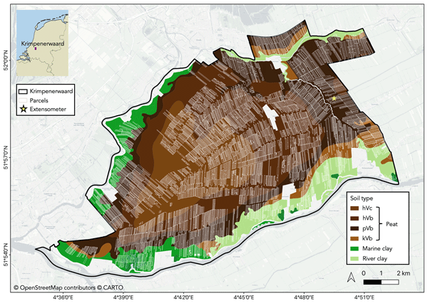
The dataset covers 3621 grassland parcels with an average size of $\sim \mathrm{1.6}\pm \mathrm{0.9}$ ha over approximately 147 km² (Fig. 2). These are permanent grassland parcels. The area is characterized by substantial peat deposits in the inner part, surrounded by marine and river clay soils in the outer part. Figure 2 shows different peat types distributed in circular shapes. These peat rings vary in their classes or subsoil materials. In the center and second inner layer, we have mesotrophic fen peat (hVc) and eutrophic fen peat (hVb), both with a clayey peaty topsoil. Further out, we have peat bogs with a sandy loam or clay cover (pVb), where a humus-rich topsoil has been developed. Similarly, some parts of the outer peat rings are peat bogs (kVb), but with a thinner or absent mineral layer on top.

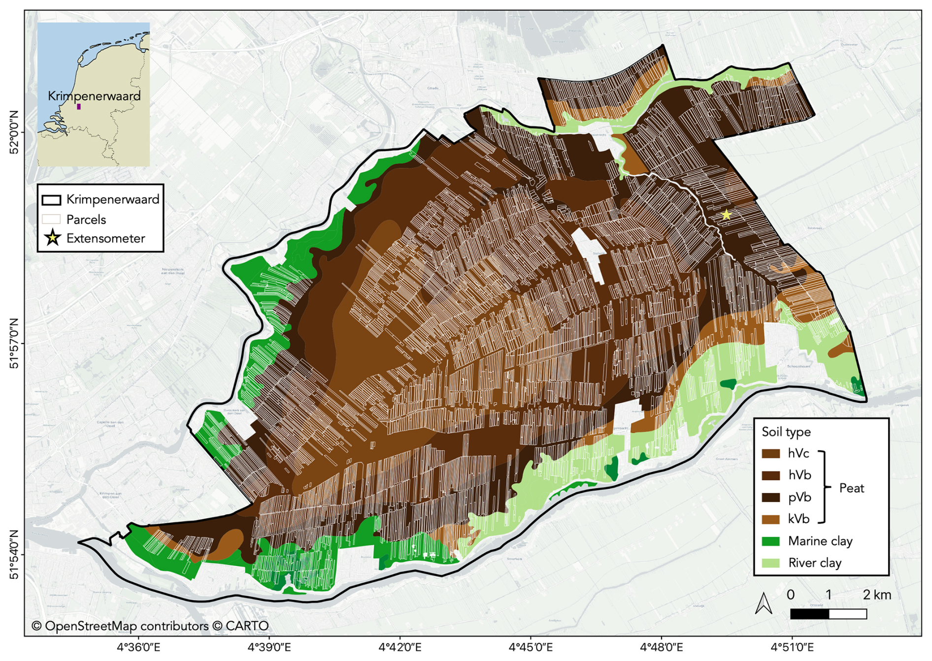
Figure 2 Krimpenerwaard study area overlayed with the soil map and parcel polygons having the estimated SPAMS10 parameters. The extensometer site is used for validation purpose.

According to the nearest meteorological stations located in Rotterdam and Cabauw, the annual mean precipitation and evapotranspiration in the study area are roughly 831 and 653 mm, respectively (KNMI, 2026). The annual precipitation-to-evapotranspiration ratio from 2015 to 2025 ranges from 0.8 to 1.7, with an average of 1.3. Several dry periods are indicated by ratios less than 1, i.e. when annual precipitation fell below annual evapotranspiration, which occurred in 2018 and 2025. In contrast, 2023 and 2024 are recorded as the wettest years over the 11 years, with precipitation approximately 1.6 times evapotranspiration and annual precipitation approximately 31 % and 17 % above the mean, respectively.

3.2 Distribution of model parameters

Figure 3a–c show the spatial distribution of the InSAR-derived soil motion parameters used to model relative surface elevation changes at the parcel level. Statistically, the median precipitation scaling factor x_P is $\sim \mathrm{7.20}\times {\mathrm{10}}^{-\mathrm{2}}$, while the median evapotranspiration scaling factor x_E is $\sim \mathrm{12.05}\times {\mathrm{10}}^{-\mathrm{2}}$. The median irreversible rate x_I across the study area is $\sim -\mathrm{2.85}\times {\mathrm{10}}^{-\mathrm{2}}\mathrm{mm}{\mathrm{d}}^{-\mathrm{1}}$. The figure also shows that some parcels still lack parameter estimates. These parcels are excluded either due to their crop type or because there are too few parcels to form a contextual group. Further methodological development is required to enable analysis in agricultural land with more complex surface dynamics.

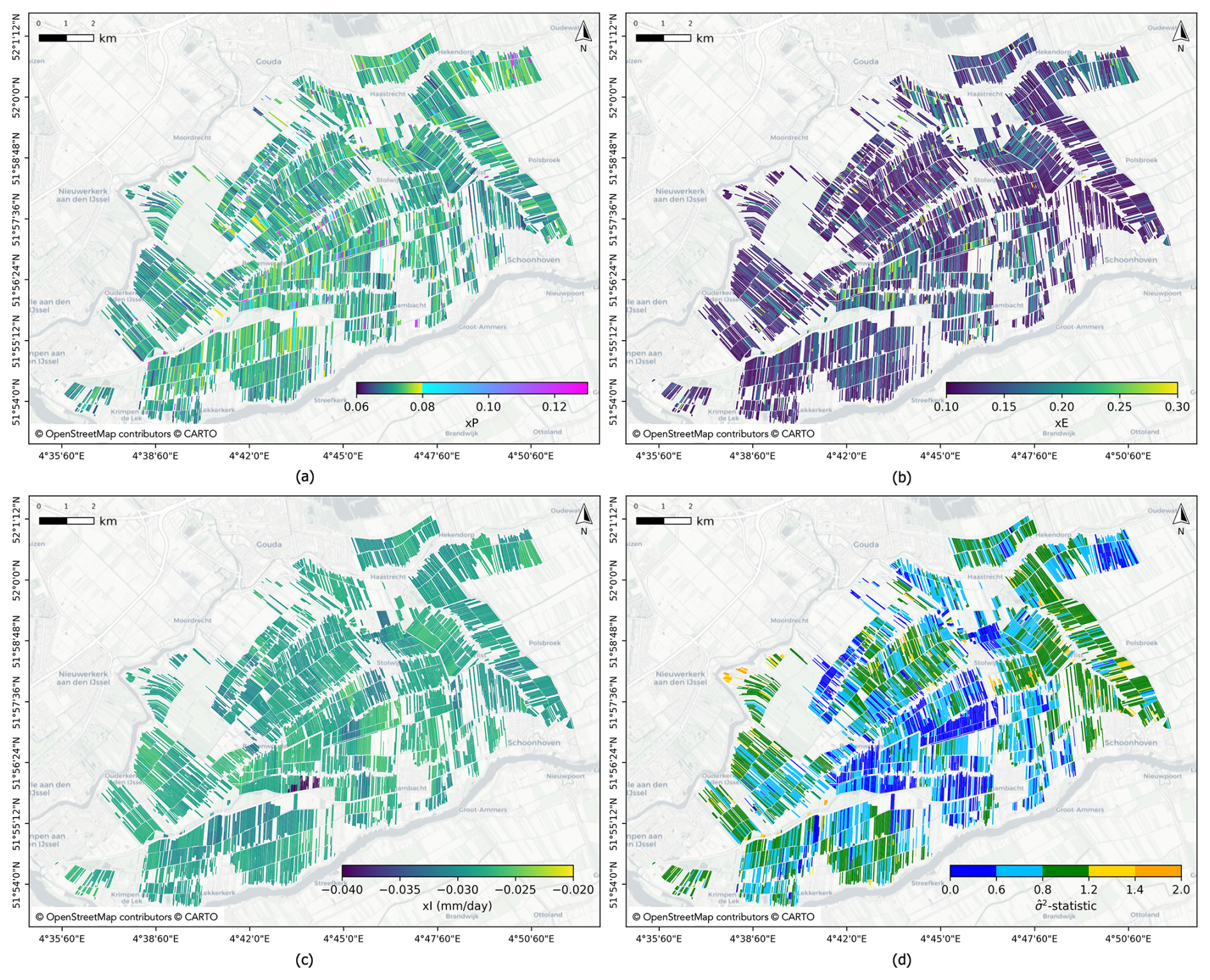
Figure 3 Spatial distributions of the SPAMS parameters for each parcel: (a) scaling factor of precipitation ${\widehat{x}}_{\mathrm{P}}$, (b) the scaling factor of evapotranspiration ${\widehat{x}}_{\mathrm{E}}$, and (c) the irreversible scaling factor ${\widehat{x}}_{\mathrm{I}}$ in mm d⁻¹. Panel (d) shows the ${\widehat{\mathit{\sigma }}}^{\mathrm{2}}$ test statistic values of each parcel. The parameters are estimated from InSAR observations from 2015 to 2025, using precipitation and evapotranspiration data from the closest meteorological station for each parcel centroid. Note that (c) alone should not be used directly to estimate the annual subsidence rates.

Figure 4 shows the distribution of the parameters across different soil types. It suggests that ${\widehat{x}}_{\mathrm{P}}$ values are similar across different soil types (Fig. 4a), with a narrow spread and a relatively homogeneous distribution. The box heights of ${\widehat{x}}_{\mathrm{E}}$ in Fig. 4b indicate a wider spread compared to ${\widehat{x}}_{\mathrm{P}}$, with less dispersion in marine clay than in other soils. It also indicates that ${\widehat{x}}_{\mathrm{E}}$ values are about twice those of ${\widehat{x}}_{\mathrm{P}}$. Given the mean precipitation-to-evapotranspiration ratio of around 1.3, parcels with smaller ${\widehat{x}}_{\mathrm{E}}$ are less susceptible to precipitation deficit. This condition implies fewer dry periods, which translates into lower annual subsidence rates, assuming a similar distribution of the ${\widehat{x}}_{\mathrm{I}}$ parameter shown in Fig. 4c. Note that the ${\widehat{x}}_{\mathrm{I}}$ parameter cannot be used directly to estimate the annual subsidence rates. It should be used together with other parameters to determine the number of dry and wet days in the time series. Once we flag the dry periods, we can compute the irreversible component and estimate the annual subsidence rates.

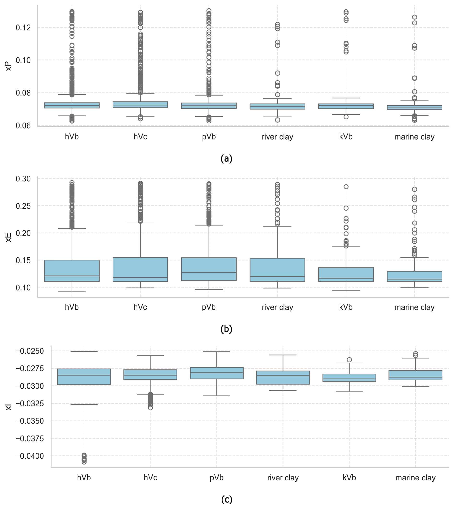
Figure 4 Boxplots of the scaling factor of precipitation ${\widehat{x}}_{\mathrm{P}}$ (a), the scaling factor of evapotranspiration ${\widehat{x}}_{\mathrm{E}}$ (b), and the irreversible scaling factor ${\widehat{x}}_{\mathrm{I}}$ in mm d⁻¹ (c) for six soil types: hVc, hVb, pVb, kVb, marine clay, and river clay, where the first four represent peat.

The quality is measured based on the ${\widehat{\mathit{\sigma }}}^{\mathrm{2}}$ test statistic to evaluate the functional and stochastic model in relation to the observations. This evaluation is computed based on the sum of squared residuals, weighted by the inverse of the variance-covariance matrix of the observations, between InSAR displacement estimates projected onto the vertical and the SPAMS elevation model, normalized by the degrees of freedom for each parcel, which is expressed as Teunissen (2024)

$$\begin{array}{}\text{(15)}& {\displaystyle }{\displaystyle }{\widehat{\underset{\mathrm{¯}}{\mathit{\sigma }}}}^{\mathrm{2}}={\displaystyle \frac{{\widehat{\underset{\mathrm{¯}}{e}}}^{\mathrm{T}}{Q}_y^{-\mathrm{1}}\widehat{\underset{\mathrm{¯}}{e}}}{m-n}},\end{array}$$

where $\widehat{\underset{\mathrm{¯}}{e}}$ is the vector of residuals between the InSAR-based relative elevation estimates and the SPAMS model, Q_y is the variance-covariance matrix of the observables where the values are described as in Eq. (14), m is total number of observations, and n is total number of estimated parameters. The ${\widehat{\mathit{\sigma }}}^{\mathrm{2}}$ test statistic values are non-negative numbers, typically ranging from 0.1 to 1.9 for the area of interest with a distribution depicted in Fig. 3d. Values close to one suggest sufficient alignment between the model and the observations. Values larger than one indicate model imperfections or an overly optimistic stochastic model. On the contrary, values significantly smaller than one indicate an overly pessimistic stochastic model (or over-parameterized functional model).

3.3 Comparison with extensometer

An additional validation is performed using an extensometer installed on one of the parcels inside the area of interest, marked by the star point in Fig. 2. This extensometer is used as reference data to evaluate both the absolute phase estimates and the model. Note that the extensometer measures only a single point, whereas the model represents the entire parcel. The parcel stretches west to east of about 1000 m long and is approximately 40 m wide. The extensometer is in the middle between the northern and southern ditches, about 20 m from each side. Figure 5 plots the extensometer data together with InSAR-based relative elevation estimates and the SPAMS model. The evaluation metrics described using RMSE and ${\widehat{\mathit{\sigma }}}^{\mathrm{2}}$ test statistic. The InSAR and SPAMS estimates yield RMSE values of approximately 8.3 and 7.1 mm, respectively, when compared to extensometer data. The calculated ${\widehat{\mathit{\sigma }}}^{\mathrm{2}}$ test statistic of roughly 0.8 suggests the modeled elevation changes are statistically adequate.

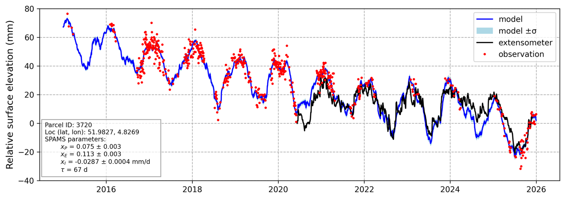
Figure 5 Comparison of relative surface elevation changes from extensometer data (black line), InSAR-based relative elevation estimates (red dots), and the SPAMS model (blue line) showing relatively similar agreement levels. The RMSE values for InSAR and SPAMS, relative to the extensometer, are approximately 8.3 and 7.1 mm, respectively. The RMSE between InSAR and SPAMS is around 4.6 mm. The ${\widehat{\mathit{\sigma }}}^{\mathrm{2}}$-statistic is roughly 0.8, indicating model adequacy.

The model shows some discrepancies relative to the extensometer; for example, in summer 2020, the extensometer records subsidence, whereas the model estimates slight uplift. Also, in 2024, the model subsides more than the extensometer. Several factors can cause these discrepancies: (i) the extensometer and the parcel do not observe the same behavior in which what occurs at one surface point may not be the same at every point within the corresponding parcel; (ii) the lack of observations, especially in summer periods, limit the model parameter estimation process and lead to undetected errors since the quality of the model is statistically propagated based on the available observations; (iii) limitations of the model in capturing surface responses to driving factors beyond meteorological conditions.

Figure 5 also shows the uncertainty of modeled displacement per epoch represented by the blue shades. This uncertainty was estimated using a Monte Carlo simulation that reconstructs different realizations from parameter sets distributed according to the covariance of the estimated parameters. The figure shows varying uncertainty, with summer periods showing higher uncertainty than winter, where the standard deviation (2σ) can reach approximately 3.6 mm. Across all parcels in the study area, the standard deviation can reach up to 12 mm. Although these values are relatively small, they remain useful indicators for assessing the effect of parameter uncertainty on the model realization. Further study is required to evaluate the stochastic model of the observations.

4 Data records

The SPAMS10 dataset over the Krimpenerwaard region in the Netherlands is available through the 4TU.ResearchData repository: https://doi.org/10.4121/dfbe9109-d058-4a64-a5b4-1cc9d9a5f836 (Lumban-Gaol et al., 2025). The main data file, stored in a parquet format, contains a set of 10 SPAMS parameters per evaluated parcel. It includes the coordinates of its center-of-mass and relevant contextual information for each parcel. The contextual information includes the identifier of the closest meteorological station and the soil code describing the shallow soil type. The meteorological station identifiers in this dataset is according to the Royal Netherlands Meteorological Institute KNMI (last access: 16 September 2026). Details about soil code can be found in the PDOK-BRO (last access: 16 September 2026) repository. A companion JSON file provides detailed schema definitions, including parameter units and interrelationships, to facilitate automated data integration and interpretation. The dataset is distributed under a Creative Commons Attribution 4.0 International (CC BY 4.0) license.

5 Code and data availability

The SPAMS10 dataset over the Krimpenerwaard region in the Netherlands is available through the 4TU.ResearchData repository: https://doi.org/10.4121/dfbe9109-d058-4a64-a5b4-1cc9d9a5f836 (Lumban-Gaol et al., 2025). The dataset is distributed under a Creative Commons Attribution 4.0 International (CC BY 4.0) license.

The computations presented in this work were done with InSAR software package, DECADE (last access: 16 September 2026), developed by the Geodesy team at Delft University of Technology. A Python implementation to create a realization of relative surface elevation using a set of estimated SPAMS10, along with utilities for loading and analyzing the SPAMS10 dataset, is available at https://github.com/TUDelftGeodesy/pyspams (last access: 16 September 2026; https://doi.org/10.5281/zenodo.22659123, Lumban-Gaol, 2026).

6 Usage notes

The SPAMS10 dataset is intended for a range of applications, including subsidence forecasting under climate change scenarios, assessment of groundwater management interventions, and gap-filling in InSAR time series analysis. The dataset is compatible with open-source geospatial analysis tools and can be readily imported into Python-based workflows using the pyspams (last access: 16 September 2026) library. Example code and integration guides are provided in the dataset documentation to support reproducible research and practical implementation.