GloSVeT: a global 0.05° monthly mean surface soil and vegetation component temperature dataset (2003–2023)

Current satellite-derived land surface temperature (LST) products represent a mixed radiative signal that integrates soil and vegetation contributions, obscuring the physical mechanisms controlling surface energy partitioning and ecosystem functioning. To overcome this limitation, this study developed the Global Soil and Vegetation Temperature dataset (GloSVeT), the first global product that simultaneously provides surface soil and vegetation component temperatures at 0.05° spatial resolution for the period 2003–2023. GloSVeT was generated using the multisource data fusion-based global surface soil and vegetation temperature retrieval (FuSVeT) method, which integrates multi-temporal MODIS observations with ERA5-Land reanalysis to improve spatial completeness, retrieval accuracy, and computational efficiency. Its performance was extensively assessed through a comprehensive evaluation framework combining internal closure check, flux-tower validation at 72 representative sites, triple collocation (TC) analysis, and physical consistency assessments. Results show that GloSVeT largely preserves the original MODIS mixed-pixel LST constraint, and achieves reliable accuracy with coefficients of determination mostly at or above 0.9 and root mean square errors generally around 2 K for both components. TC analysis further demonstrates globally consistent performance, with advantages in humid tropics and transitional ecosystems compared with reanalysis products. In addition, soil temperature anomalies are predominantly negatively correlated with soil moisture whereas vegetation temperature aligns with solar-induced fluorescence along a clear gradient from energy-limited to water-limited biomes, indicating the physical consistency of GloSVeT. Over pixels where soil and vegetation temperatures are simultaneously available, both components exhibit evident warming trends during 2003–2023, with rates of 0.44 ± 0.04 K per decade for soil temperature and 0.39 ± 0.04 K per decade for vegetation temperature. In summary, GloSVeT provides a physically consistent, observation-driven depiction of surface thermal dynamics, offering new opportunities for quantifying land–atmosphere energy exchange, monitoring ecosystem hydrothermal responses, and improving the representation of land surface processes in Earth system models. GloSVeT is publicly available at https://doi.org/10.11888/RemoteSen.tpdc.303317 (Liu and Li, 2026a) and https://doi.org/10.5281/zenodo.22724289 (Liu and Li, 2026b).

1 Introduction

Land surface temperature (LST) is a key boundary variable governing the exchange of energy and water between the land surface and the atmosphere (Li et al., 2023). It captures a broad range of surface and ecological processes, including plant physiological activity and soil moisture dynamics (Li et al., 2021; Prentice et al., 2024), and has been widely applied in drought monitoring, urban heat island assessment, climate change analysis, and ecosystem modeling (Blyth et al., 2021; Wan et al., 2021; Wang et al., 2025). However, satellite-based LST products, owing to their limited spatial resolution, generally represent a mixed radiometric signal that combines temperature contributions from multiple components within each pixel (Li et al., 2013). This mixture obscures the heterogeneity of surface thermal conditions and constrains our understanding of how different land components, particularly soil and vegetation, regulate surface energy and water fluxes. In contrast, separating LST into soil and vegetation component temperatures provides a more physical and mechanistic representation of land–atmosphere interactions (Zhan et al., 2013; Liu et al., 2020b). Component temperature datasets thus serve as essential inputs for two-source energy balance modeling (Song et al., 2020), evapotranspiration partitioning (Jiang et al., 2022), vegetation stress diagnosis (Doughty et al., 2023), and studies of climate–ecosystem coupling (García-García et al., 2023).

Over the past decades, considerable efforts have been made to estimate soil temperature at global and regional scales, resulting in two main types of products: reanalysis products and machine-learning-based datasets. Reanalysis products, such as ERA5-Land (Muñoz-Sabater et al., 2021) and GLDAS (Rodell et al., 2004), which rely on data assimilation techniques and land surface modelling, provide spatially continuous soil temperature information at multiple depths and temporal scales. Their main advantage lies in long-term continuity, global coverage, and physically consistent representation of land surface process. However, these products are generally provided at relatively coarse spatial resolutions, typically ranging from 0.10 to 0.625°, and their performance can be affected by land surface model structure, parameterization schemes, and forcing uncertainties. With the recent advances in artificial intelligence and the expansion of in situ observational networks, several machine-learning–based soil temperature datasets have been developed (Wang et al., 2026; Baumberger et al., 2024; Lembrechts et al., 2022). Compared with reanalysis products, these datasets can better exploit observational constraints and environmental covariates, and often achieve higher spatial resolutions, such as 1 km. Nevertheless, they are generally limited in regional coverage or representation of only climatological averages (Lembrechts et al., 2022; Wang et al., 2026), which constrains their broader applicability. A summary of representative soil temperature products, including their spatial and temporal coverage, resolution, target depth, methodology, and access information, is provided in Table A1. In contrast to soil temperature, no operational global product currently exists for vegetation temperature. In regions with dense vegetation cover, air temperature is often used as a proxy because of its strong coupling with canopy temperature (Li et al., 2001; Zhan et al., 2011; Rutter et al., 2023), while some studies have directly substituted LST for vegetation temperature when deriving vegetation physiological parameters such as evapotranspiration (Ma et al., 2022) or gross primary productivity (GPP) (Sims et al., 2008; Tang et al., 2021). Consequently, there remains a lack of long-term, high-resolution datasets that simultaneously provide soil and vegetation component temperatures over the same regions under diverse environmental conditions.

In the context of thermal infrared (TIR) remote sensing, component temperature separation enables the decomposition of the LST of a mixed pixel into the temperatures of its constituent land surface components (Zhan et al., 2013). These component temperatures have a specific radiometric meaning: they represent the thermal states of the visible vegetation and soil/background surfaces within the sensor field of view. Because real land surfaces have complex three dimensional structures, these radiometric temperatures are not necessarily equivalent to the thermal state of shaded soil beneath canopies or to that of the entire canopy. Nevertheless, they provide an effective and physically interpretable way for constructing a dataset that simultaneously characterizes the thermal behavior of soil and vegetation components. Methodologically, this process involves solving an ill-posed problem, i.e., estimating soil and vegetation component temperatures from a single retrieved apparent LST. Accordingly, a variety of algorithms have been developed to exploit additional temporal (Zhao et al., 2014), spatial (Song et al., 2015; Zhan et al., 2011), angular (Li et al., 2001; Lu et al., 2025), or spectral (Lundquist et al., 2018) information from satellite observations. Given the inherent limitations of each individual approach, several hybrid methods (Bian et al., 2020; Liu et al., 2020b) have been proposed to make full use of the complementary advantages of different types of information, advancing component temperature retrieval from theoretical algorithm development toward practical large-scale implementations. To further overcome the observational constraints of satellite data, Liu et al. (2025) developed a multisource data Fusion-based global surface Soil and Vegetation Temperature retrieval (FuSVeT) method, which integrates multi-temporal MODIS observations to increase the number of equations and incorporates ERA5-Land reanalysis data to reduce the unknown parameters. As a result, the FuSVeT framework delivers higher retrieval accuracy, more complete spatial coverage, and markedly improved computational efficiency compared with previous satellite-only approaches, providing a promising foundation for producing long-term global soil and vegetation component temperature datasets.

A further challenge in producing reliable component temperature products lies in the lack of effective validation strategies. Widely used ground-based measurement networks, such as the Surface Radiation Budget Network (SURFRAD, https://www.esrl.noaa.gov/gmd/grad/surfrad/, last access: 25 June 2026), the AmeriFlux network (https://ameriflux.lbl.gov/, last access: 25 June 2026) and the Karlsruhe Institute of Technology stations (KIT, https://www.imkasf.kit.edu/english/skl_stations.php, last access: 25 June 2026), generally record either surface skin or air temperature rather than distinct soil and canopy components (He et al., 2025). Consequently, pixel-scale observations of soil and vegetation temperatures are extremely scarce, making direct evaluation of satellite-derived results nearly impossible. Some studies have attempted to identify pure pixels from higher resolution satellite data and used their LSTs as reference values to assess coarse resolution retrievals (Liu et al., 2020a, 2025). However, due to the sparse distribution of pure pixels, such localized comparisons cannot provide a comprehensive or statistically robust evaluation at continental or global scales. Examination of the spatiotemporal coherence of other temperature products, for instance through spatial gradients or temporal variation trends (Liu et al., 2025; Wang et al., 2026), offers an alternative means of cross-validation, but these approaches generally yield only qualitative assessments. In contrast, robust non-reference validation frameworks have been developed to evaluate dataset reliability without relying on absolute ground truth. Among them, the triple collocation (TC) provides a practical tool for quantifying the relative errors and mutual consistency among three independent datasets that observe the same target variable (Gruber et al., 2016; Park et al., 2023; Stoffelen, 1998; Wei et al., 2024). Although TC was originally designed for other geophysical variables such as soil moisture and precipitation, its demonstrated robustness and scalability make it particularly promising for evaluating component temperature products, offering a pathway toward large-scale, physically consistent assessments of spatiotemporal stability, internal coherence, and overall applicability.

To address these challenges, this study presents GloSVeT, the first global dataset of monthly mean surface soil and vegetation component temperatures from 2003 to 2023 at 0.05° spatial resolution. The dataset is generated using the previously developed FuSVeT framework, which is expanded from algorithm development to global implementation through multi-source integration and large-scale automated processing. Beyond dataset production, this study further establishes a comprehensive evaluation strategy tailored to component temperature products, combining internal closure check of the decomposition–reconstruction process, site-based validation against in situ temperature observations from a comprehensive network, TC analysis incorporating reanalysis soil and air temperatures, indicator-based consistency assessment with soil moisture and solar-induced fluorescence (SIF), and examination of seasonal spatiotemporal consistency. This multi-perspective assessment helps address the long standing difficulty of evaluating component temperatures in the absence of direct global ground truth. As the first long-term, high-resolution global product that simultaneously represents soil and vegetation component temperatures, GloSVeT provides a valuable foundation for quantifying land–atmosphere energy exchange, partitioning evapotranspiration, and improving ecosystem and climate models. The dataset is freely available at https://doi.org/10.11888/RemoteSen.tpdc.303317 (Liu and Li, 2026a) and https://doi.org/10.5281/zenodo.22724289 (Liu and Li, 2026b).

2 Data

2.1 Data used for GloSVeT generation

To generate the GloSVeT, multiple datasets from satellite observations and reanalysis products were jointly employed to provide thermal, structural, and ancillary information (Table 1). These inputs ensure the physical consistency and global completeness of the GloSVeT production framework.

Table 1 Data used for the generation of the GloSVeT product.

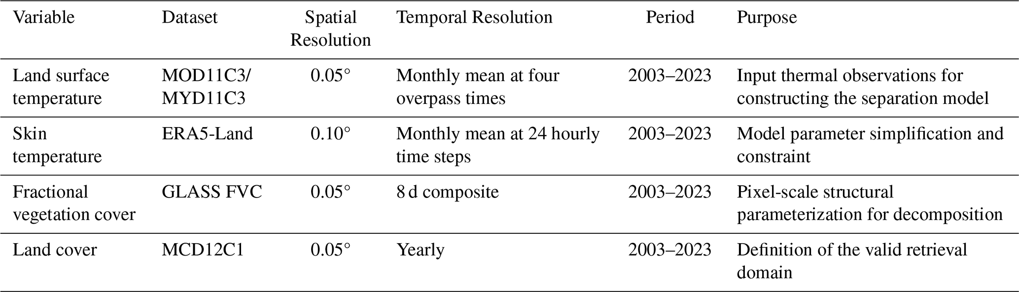
The long-term MODIS record provides more than two decades of globally consistent observations, making it one of the most widely used and physically robust datasets for monitoring land surface thermal dynamics (Li et al., 2023). Therefore, this study employs the MODIS Collection 6.1 monthly LST products, namely MOD11C3 (Terra) and MYD11C3 (Aqua), which provide global monthly mean LSTs at nominal observation times of 10:30/22:30 local solar time for Terra and 13:30/01:30 for Aqua, respectively, with a spatial resolution of 0.05°. Both datasets are generated using the standard day/night algorithm (Wan and Li, 1997) and further filled with data derived from the generalized split window algorithm (Wan and Dozier, 1996) to enhance spatial completeness. Within the FuSVeT framework, these two products serve as the primary thermal inputs, providing four representative instantaneous observations per month. These observations, together with the continuous diurnal cycle information derived from ERA5-Land hourly skin temperature, are used to construct the monthly mean diurnal cycle (MDC) model, which forms the basis for separating soil and vegetation component temperatures.

To support the global generation of GloSVeT, the skin temperature variable from the ERA5-Land reanalysis dataset was employed to simplify model parameters and constrain the retrieval of soil and vegetation component temperatures. The ERA5-Land product provides physically consistent and spatially continuous estimates of the surface thermal state, derived through data assimilation and land surface modeling (Muñoz-Sabater et al., 2021). It offers hourly skin temperature fields aggregated into monthly averages at a spatial resolution of 0.10°, with long-term continuity from 1950 to the present, ensuring complete temporal coverage and global consistency. In this study, the ERA5-Land skin temperature data were resampled to 0.05° using the nearest neighbour method to maintain spatial consistency with the MODIS LST inputs.

Fractional Vegetation Cover (FVC) was used to characterize the sub-pixel composition of soil and vegetation components, which is essential for temperature decomposition. The Global Land Surface Satellite (GLASS) FVC product is derived from MODIS surface reflectance data using high-spatial-resolution reference FVC and the general regression neural network approach (Jia et al., 2015). This product has been extensively validated and demonstrates accuracy comparable to other global FVC datasets, while offering superior spatial and temporal continuity. In this study, the 8 d 0.05° GLASS FVC product was employed and aggregated to monthly means to represent pixel-level vegetation structure, ensuring spatiotemporal consistency with the MODIS LST inputs and facilitating the global generation of GloSVeT.

Since the ERA5-Land product provides seamless global coverage without explicit distinction between land and non-land surfaces, additional land cover information was required to define the valid retrieval domain and to identify surfaces that warrant cautious interpretation (Liu et al., 2025). To ensure consistency with the MODIS-based inputs, this study employed the MODIS Collection 6.1 Land Cover Type Yearly Global 0.05° product (MCD12C1), which provides annual global land cover classification derived from MODIS surface reflectance data using the International Geosphere Biosphere Programme (IGBP) scheme (Sulla-Menashe et al., 2019). Pixels identified as water bodies (IGBP type = 17) or permanent snow/ice (IGBP type = 15) were excluded based on the MCD12C1 land cover map. By contrast, urban and built-up pixels (IGBP type = 13) were retained for spatial completeness, since such pixels may contain mixed vegetation and non-vegetation background signals at the 0.05° scale.

2.2 Data used for GloSVeT evaluation

To evaluate the accuracy, consistency, and physical reliability of the GloSVeT dataset, multiple independent data sources were employed, including ground-based observations, reanalysis products, and environmental indicators (Table 2). These datasets support three complementary validation strategies: site-based comparison, TC analysis, and indicator-based consistency assessment.

Table 2 Data used for the evaluation of the GloSVeT product.

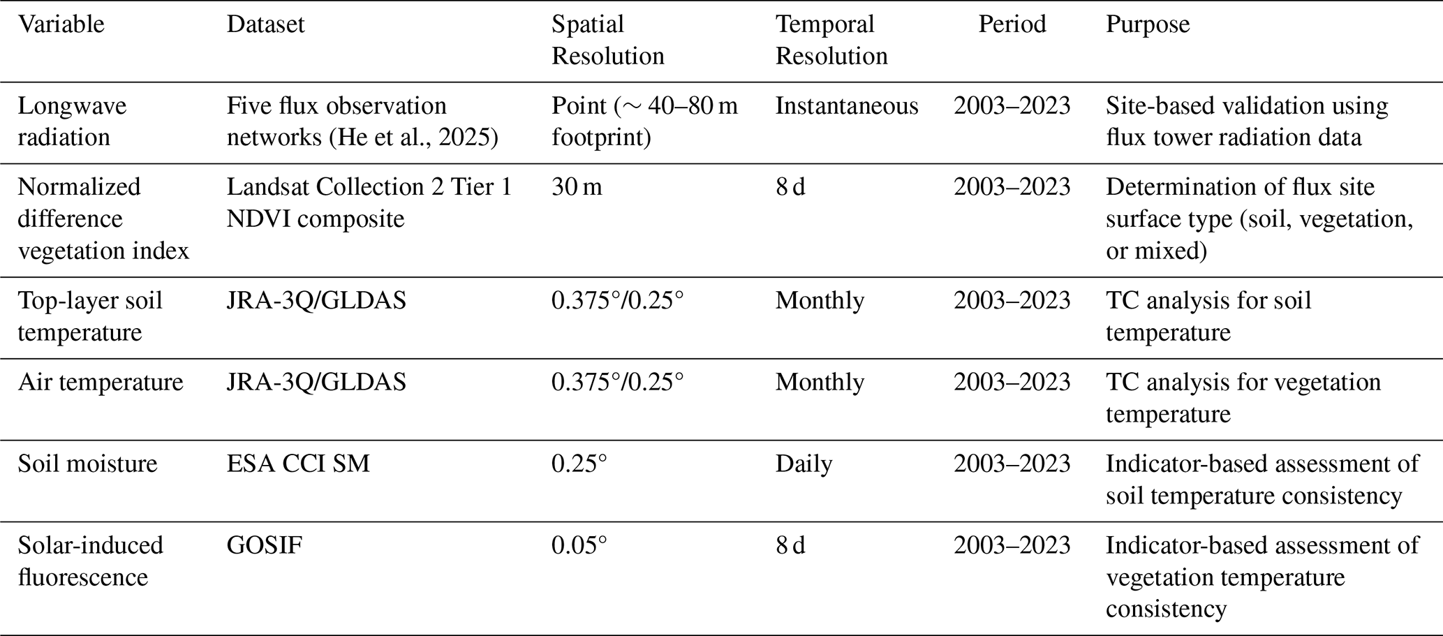
The temperature-based validation approach is the most straightforward means of assessing the accuracy of temperature products, as it directly compares satellite-retrieved temperatures with concurrent ground measurements (Li et al., 2023). Using random forest modelling and Landsat LST data, He et al. (2025) systematically evaluated the spatial representativeness of 211 flux sites from five observation networks worldwide, and identified 46, 36, 49, and 62 sites with strong spatial representativeness across multiple scales (1, 3, 5, and 10 km) for spring, summer, autumn, and winter, respectively. Detailed information on the selected sites and their spatial distribution can be found in Table II and Fig. 6 of He et al. (2025). Following their findings, this study adopted these season-specific site sets and collected available upward and downward longwave radiation records from 2003 to 2023 for the union of these sites, comprising 72 unique flux sites in total. The collected radiation records were then used to calculate site-level instantaneous LST according to the following equation (Xing et al., 2021).

$$\begin{array}{}\text{(1)}& T_{\mathrm{i}}={\left[{\displaystyle \frac{L_{\mathrm{u}}-(\mathrm{1}-{\mathit{\epsilon }}_{\mathrm{b}})\times L_{\mathrm{d}}}{\mathit{\sigma }\times {\mathit{\epsilon }}_{\mathrm{b}}}}\right]}^{\mathrm{1}/\mathrm{4}}\end{array}$$

where T_i is the instantaneous temperature; L_u and L_d are the upwelling and downwelling longwave radiation, respectively; σ is the Stefan–Boltzmann constant ($\mathrm{5.670373}\times {\mathrm{10}}^{-\mathrm{8}}$ $\mathrm{W}{\mathrm{m}}^{-\mathrm{2}}{\mathrm{K}}^{-\mathrm{4}}$); and ε_b is the broadband emissivity, calculated using spectral emissivities from the Cooperative Institute for Meteorological Satellite Studies (CIMSS) baseline-fit emissivity database (http://cimss.ssec.wisc.edu/iremis/, last access: 24 August 2025) as input, following a linear conversion method (Cheng et al., 2013). Subsequently, all instantaneous LST estimates, regardless of clear-sky or cloudy conditions, were averaged to derive the true monthly mean LST (Xing et al., 2021). This tower-derived radiometric LST was used as an approximate component temperature reference only when the tower footprint was dominated by either bare soil or vegetation. Typically, the effective observational footprints of these flux towers range from 40 to 80 m in diameter. To identify near pure surface conditions, we additionally used the Landsat Collection 2 Tier 1 Level-2 8 d 30 m normalized difference vegetation index (NDVI) composite (https://developers.google.com/earth-engine/datasets/catalog/LANDSAT_COMPOSITES_C02_T1_L2_8DAY_NDVI, last access: 26 August 2025). Specifically, the 8 d NDVI values at each site were aggregated to monthly means. The corresponding tower-derived LST records were used as soil temperature references when NDVI≤0.1 and as vegetation temperature references when NDVI≥0.7, whereas records with intermediate NDVI values were excluded from the component temperature validation.

Because long-term, observation-based soil and vegetation temperature datasets with global coverage are currently unavailable, two reanalysis datasets, JRA-3Q (Kosaka et al., 2024) and GLDAS (Rodell et al., 2004), were used as physically related comparison datasets for the TC analysis. The JRA-3Q product provides monthly averaged variables at a spatial resolution of 0.375°, while GLDAS offers 0.25° resolution. To maximize consistency with the GloSVeT soil temperature, only the top-layer soil temperature was used from both datasets. Specifically, the monthly mean soil temperature at level 1 layer (0–2 cm) from JRA-3Q and the SoilTMP0_10cm_inst variable (0–10 cm) from GLDAS were employed. Although these variables differ in their effective soil depth and are not identical to the TIR surface soil component temperature retrieved by GloSVeT, they are physically related near-surface soil thermal variables and can therefore serve as reasonable proxy datasets for evaluating relative consistency within the TC framework. For vegetation temperature, near-surface air temperature was used as a proxy in densely vegetated regions, given the strong coupling between canopy temperature and near-surface air temperature through land–atmosphere heat exchange (Li et al., 2001; Zhan et al., 2011; Rutter et al., 2023). Accordingly, the monthly mean 2 m air temperature from JRA-3Q and the Tair_f_inst variable from GLDAS were used for the vegetation-temperature TC analysis. For consistency in spatial support, GloSVeT soil and vegetation temperatures, GLDAS soil temperature and air temperature, and GLASS FVC were aggregated to the 0.375° JRA-3Q grid using an area-weighted method. The aggregated GLASS FVC was further used to identify densely vegetated pixels (FVC≥0.8) for the evaluation of vegetation temperature.

To evaluate the physical consistency of GloSVeT, we examined the relationships between soil temperature and soil moisture, as well as between vegetation temperature and SIF. These analyses were designed to assess whether the spatial and temporal variations in GloSVeT are consistent with the expected energy–water–carbon interactions derived from theory and independent observations. For this purpose, we used the European Space Agency Climate Change Initiative Soil Moisture (ESA CCI SM) product, which provides a long-term, quality-controlled global record (1978–present) generated through a multi-sensor merging algorithm (Dorigo et al., 2017; Gruber et al., 2019). The dataset offers daily global coverage at 0.25° spatial resolution. In this study, the SM data were averaged to monthly means, and the GloSVeT soil temperatures were aggregated to 0.25° to ensure spatial comparability. For vegetation, we used the GOSIF dataset, a global SIF product derived from discrete OCO-2 soundings, MODIS observations, and meteorological reanalysis inputs using a data-driven approach (Li and Xiao, 2019). GOSIF provides 8 d SIF estimates at 0.05° resolution for the period 2000–2024 and shows strong agreement with GPP from 91 FLUXNET sites, i.e., the coefficient of determination (R²) =0.73 and p<0.001. In this study, the SIF data were aggregated to monthly means to match the temporal scale of GloSVeT and used to examine the correspondence between vegetation temperature and photosynthetic activity.

3 Method

3.1 FuSVeT

In the FuSVeT framework, the temporal variations of soil and vegetation temperatures at the monthly scale are described using an MDC model. In this study, the well-established GOT09 model (Göttsche and Olesen, 2009) was adopted to represent sub-daily temperature dynamics, as expressed in Eqs. (2)–(6).

$$\begin{array}{}\text{(2)}& {\displaystyle }\left\{\begin{array}{l}{T}_{\text{day}}\left(t\right)=\\ T_{\mathrm{0}}+T_{\mathrm{a}}\cos \left({\mathit{\theta }}_{\mathrm{z}}\right){\cos }^{-\mathrm{1}}\left({\mathit{\theta }}_{\mathrm{z},\text{min}}\right)\cdot e^{[m_{\text{min}}-m({\mathit{\theta }}_{\mathrm{z}}\left)\right]\mathit{\tau }},t<t_{\mathrm{s}}\\ T_{\text{night}}\left(t\right)=\\ T_{\mathrm{0}}+\mathit{\delta }T+\left[T_{\mathrm{a}}\cos \right({\mathit{\theta }}_{\text{zs}}\left){\cos }^{-\mathrm{1}}\right({\mathit{\theta }}_{\mathrm{z},\text{min}})\\ \cdot e^{[m_{\text{min}}-m({\mathit{\theta }}_{\text{zs}}\left)\right]\mathit{\tau }}-\mathit{\delta }T]e^{\frac{-\mathrm{12}}{\mathit{\pi }k}(\mathit{\theta }-{\mathit{\theta }}_{\mathrm{s}})},t\ge t_{\mathrm{s}}\end{array}\right.\text{(3)}& {\displaystyle }\mathit{\theta }={\displaystyle \frac{\mathit{\pi }}{\mathrm{12}}}(t-t_{\mathrm{m}})\text{(4)}& {\displaystyle }{\mathit{\theta }}_{\mathrm{z}}=\arccos \left(\sin \right(\mathit{\delta }\left)\sin \right(\mathit{\varphi })+\cos (\mathit{\delta }\left)\cos \right(\mathit{\varphi }\left)\cos \right(\mathit{\theta }\left)\right)\text{(5)}& {\displaystyle }m\left({\mathit{\theta }}_{\mathrm{z}}\right)=-{\displaystyle \frac{R_{\mathrm{E}}}{H}}\cos \left({\mathit{\theta }}_{\mathrm{z}}\right)+\sqrt{{\left[{\displaystyle \frac{R_{\mathrm{E}}}{H}}\cos \left({\mathit{\theta }}_{\mathrm{z}}\right)\right]}^{\mathrm{2}}+\mathrm{2}{\displaystyle \frac{R_{\mathrm{E}}}{H}}+\mathrm{1}}\text{(6)}& {\displaystyle }k={\displaystyle \frac{\mathrm{12}}{\mathit{\pi }{\displaystyle \frac{\mathrm{d}{\mathit{\theta }}_{\mathrm{z}}\left({\mathit{\theta }}_{\mathrm{s}}\right)}{\mathrm{d}\mathit{\theta }}}}}{\displaystyle \frac{\cos \left({\mathit{\theta }}_{\text{zs}}\right)-{\displaystyle \frac{\mathit{\delta }T}{T_{\mathrm{a}}}}{\displaystyle \frac{\cos \left({\mathit{\theta }}_{\mathrm{z},\text{min}}\right)}{e^{(m_{\text{min}}-m({\mathit{\theta }}_{\text{zs}}\left)\right)\mathit{\tau }}}}}{\sin \left({\mathit{\theta }}_{\text{zs}}\right)+\mathit{\tau }\cos \left({\mathit{\theta }}_{\text{zs}}\right){\displaystyle \frac{\partial m\left({\mathit{\theta }}_{\text{zs}}\right)}{\partial {\mathit{\theta }}_{\mathrm{z}}}}}}\end{array}$$

where T_day(t) and T_night(t) denote the day and night temperature variations at time t, respectively; T₀ is the temperature around sunrise; T_a is the diurnal temperature amplitude; t_m is the time of maximum temperature; t_s is the time marking the onset of free attenuation, representing the transition between daytime heating and nighttime cooling; τ is the atmospheric transmittance; δT is the day-to-day change of residual temperature; θ is the thermal hour angle; θ_z is the solar zenith angle; θ_z,min is the minimum solar zenith angle and can be calculated using Eq. (4) at θ=0; m is the relative air mass; m_min is the minimum relative air mass, and can be obtained using Eq. (5) at ${\mathit{\theta }}_{\mathrm{z}}={\mathit{\theta }}_{\mathrm{z},\text{min}}$; θ_s is the thermal hour angle for t=ts; θ_zs is the thermal zenith angle derived from Eq. (4) at θ=θs; R_E is the radius of the Earth, and H is the scale height of the atmosphere. This model contains six free parameters: T₀, T_a, t_m, t_s, δT, and τ.

Based on geometrical theory and the MDC model, the relationship between LST and two component temperatures can be expressed as:

$$\begin{array}{}\text{(7)}& \begin{array}{rl}T& \left(t\right)=\\ & {\left[{\displaystyle \frac{\begin{array}{l}\text{fvc}\cdot {\mathit{\epsilon }}_{\mathrm{v}}\cdot {\left[\text{MDC}\left(T_{\mathrm{0},\mathrm{v}},T_{\mathrm{a},\mathrm{v}},t_{\mathrm{m},\mathrm{v}},t_{\mathrm{s},\mathrm{v}},\mathit{\delta }{T}_{\mathrm{v}},\mathit{\tau }\right)\right]}^{\mathrm{4}}\\ +\left(\mathrm{1}-\text{fvc}\right)\cdot {\mathit{\epsilon }}_{\mathrm{s}}\cdot {\left[\text{MDC}\left(T_{\mathrm{0},\mathrm{s}},T_{\mathrm{a},\mathrm{s}},t_{\mathrm{m},\mathrm{s}},t_{\mathrm{s},\mathrm{s}},\mathit{\delta }{T}_{\mathrm{s}},\mathit{\tau }\right)\right]}^{\mathrm{4}}\end{array}}{\text{fvc}\cdot {\mathit{\epsilon }}_{\mathrm{v}}+(\mathrm{1}-\text{fvc})\cdot {\mathit{\epsilon }}_{\mathrm{s}}}}\right]}^{\mathrm{0.25}}\end{array}\end{array}$$

where T is the LST for a mixed pixel; the subscripts s and v represent the MDC parameters for soil temperature and vegetation temperature, respectively; ε_v and ε_s are the broadband emissivities for vegetation component and soil component, set to 0.98 and 0.95 in this study; fvc is the fractional vegetation cover. Accordingly, the retrieval of soil and vegetation temperatures becomes equivalent to solving for the eleven MDC parameters, i.e., T_0,s, T_a,s, t_m,s, t_s,s, δT_s, T_0,v, T_a,v, t_m,v, t_s,v, δT_v, and τ.

The core principle of FuSVeT is to partition all MDC parameters into seven temperature-independent (t_m,s, t_s,s, δT_s, t_m,v, t_s,v, δT_v, and τ) and four temperature-dependent groups (T_0,s, T_a,s, T_0,v, and T_a,v), and solve them through a multi-source data fusion strategy to ensure physical consistency and spatial completeness. Specifically, temporally dense reanalysis data are used both to directly estimate the temperature-independent parameters and to provide initial values and physical constraints for the temperature-dependent parameters. The temperature-dependent parameters are subsequently optimized using temporally sparse satellite observations. Further methodological details can be found in Liu et al. (2025).

Figure 1 Workflow for generating the GloSVeT dataset using the FuSVeT method.

3.2 Generation of GloSVeT using the FuSVeT method

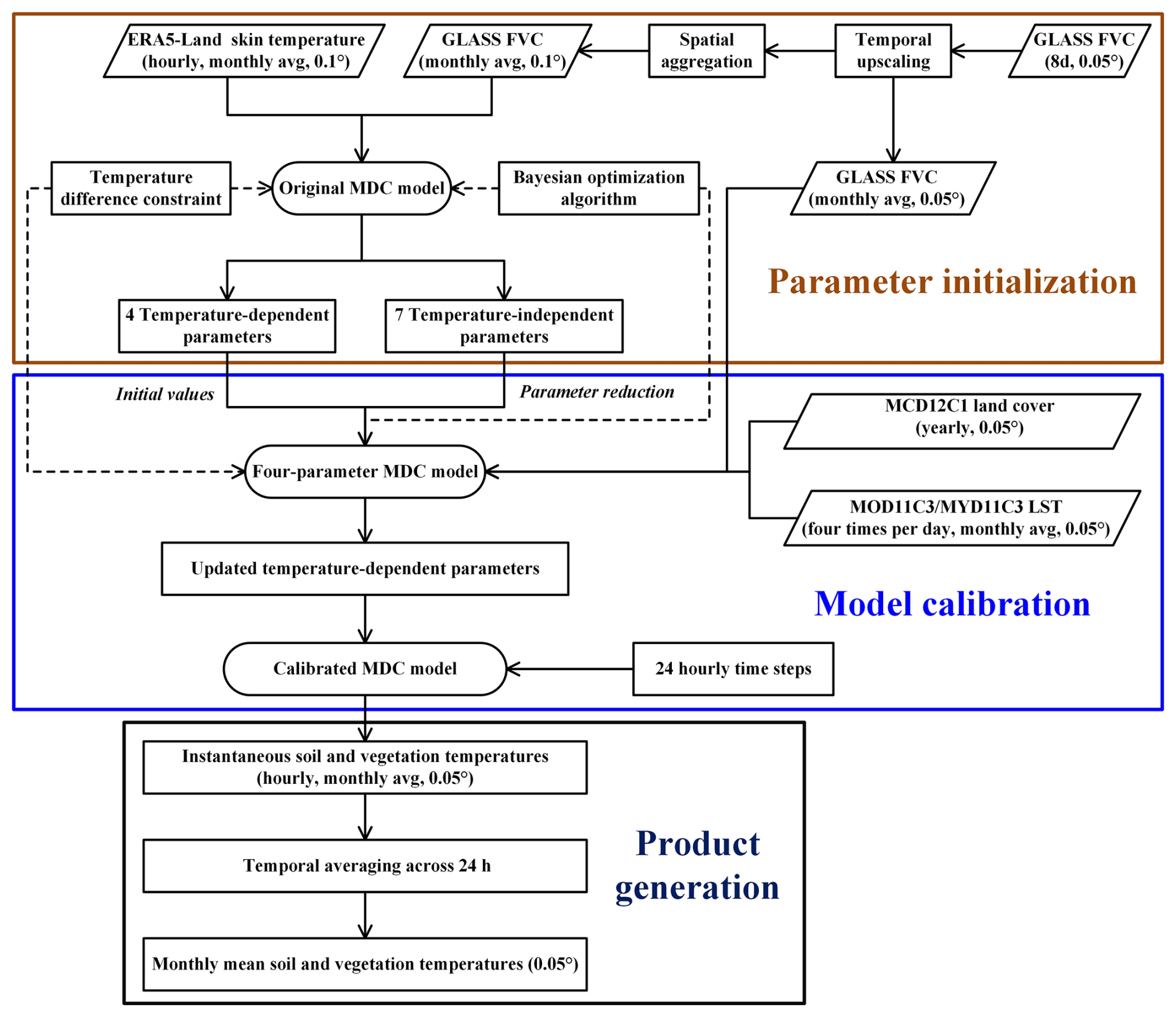
The overall technical workflow for generating the GloSVeT dataset is illustrated in Fig. 1. First, the parameter initialization was conducted at 0.10° spatial resolution using ERA5-Land skin temperature and monthly GLASS FVC data after spatial and temporal upscaling. These datasets were jointly employed to estimate seven temperature-independent and four temperature-dependent parameters within the original MDC model. To ensure physical realism, a temperature difference constraint between soil and vegetation components (−10 to 30 K) was imposed. Considering this constraint and the need for robust parameter estimation, the parameters were solved using a Bayesian optimization algorithm rather than the conventional Levenberg–Marquardt method (Liu et al., 2020b). The retrieved parameters were subsequently mapped to the 0.05° grid by uniformly assigning each 0.10° estimate to its corresponding 2×2 finer pixels. Then, model calibration was performed to further introduce satellite observation constraints and improve the retrieval accuracy of soil and vegetation component temperatures. Because only four MODIS LST retrievals at the overpass times are available for each month, directly solving all 11 parameters of the MDC model would lead to underdetermination and instability. Therefore, parameter reduction was applied by retaining the seven temperature independent parameters initialized from ERA5-Land, while only the four temperature dependent parameters were optimized using the 0.05° GLASS FVC and the MOD11C3/MYD11C3 monthly LST retrievals. The temperature difference constraint and the Bayesian optimization algorithm were also imposed during the calibration process. This step enables the resulting MDC model to retain the continuous diurnal cycle shape information provided by ERA5-Land as well as being directly constrained by MODIS LST in terms of temperature level. Finally, using this calibrated model, 24 hourly temperature steps were simulated to derive instantaneous soil and vegetation temperatures, which were then averaged temporally to obtain the final monthly mean component temperatures (Hong et al., 2022).

To enhance computational efficiency and retrieval accuracy, several technical refinements were implemented. First, the MCD12C1 land cover dataset was used to exclude non-vegetated pixels such as water bodies and permanent snow or ice, thereby reducing computational load and improving the robustness of the results. Second, Bayesian optimization is computationally intensive since it needs to iteratively build a probabilistic surrogate of the objective function and sequentially sample promising regions of the parameter space to identify the parameter set that minimizes the reconstruction error (Pelikan, 2005). To determine an appropriate iteration number, we conducted a convergence test using the July 2023 data across different FVC bins. The result from 10 000 iterations was used as the reference solution, and the retrievals obtained with fewer iterations were compared against this reference. As shown in Fig. A1, after 2000 iterations, further increasing the iteration number led only to gradual improvements. Therefore, the iteration number was set to 2000 as a practical balance between retrieval stability and computational efficiency. Finally, because errors in the MYD11C3 nighttime viewing time are known to introduce artificial patterns over the region of 20–30° E (see Figs. 8a and 9a in Liu et al., 2025), a correction was applied to the nighttime viewing time layer. Specifically, when the nighttime viewing time exceeded its theoretical range of 00:00–03:00 LT, it was replaced by the corresponding daytime viewing time shifted by 12 h under the 24 h clock. This correction was applied only to the viewing time information and did not modify the MYD11C3 LST values.

3.3 Evaluation and consistency analysis

To examine whether GloSVeT preserves the original mixed-pixel LST signal and to quantify potential structural residuals introduced during the separation process, an internal closure check was first performed. Specifically, based on Eq. (7), the calibrated MDC model was used to reconstruct mixed-pixel LSTs at the four MODIS overpass times. The closure residual was defined as the difference between the reconstructed LST and the corresponding original MODIS LST. For each month and each MODIS overpass time during 2003–2023, global RMSE and bias were calculated using all valid pixels. The resulting monthly global RMSE and bias statistics were used to assess the long-term internal closure of the decomposition–reconstruction process and its dependence on MODIS overpass time, rather than to provide an independent validation of component temperature accuracy.

The TC analysis was applied to quantify the relative random uncertainties in soil and vegetation temperatures without relying on in situ measurements. This method assumes that three independent datasets describe the same geophysical variable through linear relationships and that their random errors are mutually uncorrelated (Gruber et al., 2016; Park et al., 2023; Stoffelen, 1998). By exploiting the covariance structure among the three datasets, TC estimates dataset-specific random errors and their relative consistency with respect to an unknown target signal. In this study, TC was implemented to evaluate the reliability of GloSVeT against JRA-3Q and GLDAS for both soil and vegetation component temperatures. The analysis was conducted on a monthly basis from 2003 to 2023 using deseasonalized and detrended monthly anomalies for each dataset, obtained by removing the multi-year climatological mean for each calendar month and then the linear trend from each time series. This preprocessing minimized the influence of seasonal cycles and long-term trends, thereby emphasizing temporal co-variability among datasets. The resulting TC-based correlation coefficients provide spatially explicit diagnostics of relative reliability and spatiotemporal stability. It should be noted that these TC-based correlation coefficients are not direct measures of absolute accuracy against a known ground truth, but rather indicators of where GloSVeT shows stronger or weaker agreement with independent datasets under the TC assumptions.

An anomaly based correlation analysis was conducted to assess whether the temporal dynamics of GloSVeT are physically consistent with hydrological processes and photosynthetic activity. For the soil component, correlations were calculated between soil temperature anomalies and soil moisture anomalies for seven monthly lag conditions, namely −3, −2, −1, 0, +1, +2, and +3 months. Positive lags were defined as soil temperature anomalies preceding soil moisture anomalies, whereas negative lags indicate the opposite temporal ordering. These lagged correlations were used to identify the monthly window in which the two variables showed the strongest association, rather than to estimate an exact physical response time. For each valid pixel, only lagged correlations passing the significance test (p<0.05) were retained as candidates. If only one candidate lag was identified, it was selected directly. If multiple candidate lags were identified, the lag with the largest absolute correlation coefficient was selected as the best lag only when its absolute correlation exceeded the second largest absolute correlation by at least 0.05. The retained best lag and its corresponding correlation coefficient were then used in the subsequent analyses. For the vegetation component, correlations between vegetation temperature anomalies and SIF anomalies were examined to determine whether temperature fluctuations correspond to variations in photosynthetic activity. The analysis was restricted to the growing season, defined as the period when the climatological mean SIF exceeded its 30th percentile within the annual cycle and persisted for at least two consecutive months. This restriction ensures that the temperature–SIF relationships reflect periods of active vegetation functioning.

4 Results

4.1 Internal closure check

Figure 2 summarizes the internal closure check for GloSVeT. Overall, the reconstructed mixed-pixel LSTs were reasonably consistent with the original MODIS LST values at the four overpass times. The monthly global RMSEs generally ranged from approximately 1.2 to 2.0 K, while the bias values mostly remained within about ±1 K. The relatively compact boxplots further suggest that the closure errors were temporally stable during 2003–2023, with RMSE variations generally within about 0.2–0.5 K and bias variations within about 0.4–0.6 K.

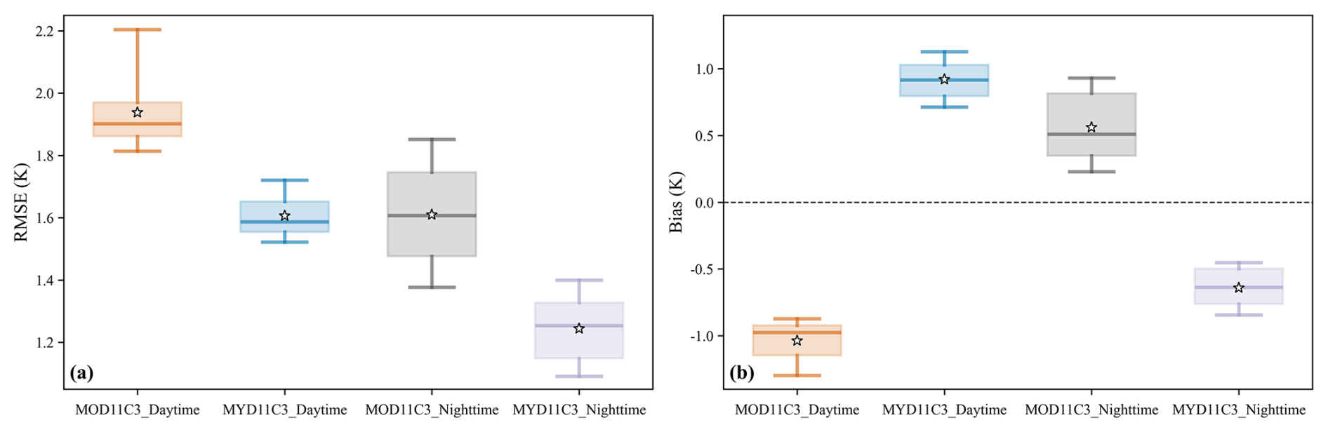
Figure 2 Internal closure check of GloSVeT. Boxplots show the distributions of monthly global (a) RMSE and (b) Bias between reconstructed mixed-pixel LST and the corresponding original MODIS LST during 2003–2023 at the four MODIS overpass times. Stars denote the mean values, and the dashed line in panel (b) indicates zero Bias.

The closure residuals also exhibited clear overpass-time dependence. In terms of RMSE, MYD11C3_Nighttime (i.e., 01:30 nominal local time) yielded the smallest closure error, with a median RMSE of about 1.24 K, whereas MOD11C3_Daytime (i.e., 10:30 nominal local time) had the largest error, with a median RMSE close to 1.94 K. MYD11C3_Daytime (i.e., 13:30 nominal local time) and MOD11C3_Nighttime (i.e., 22:30 nominal local time) had intermediate RMSEs, both around 1.61 K. The bias statistics revealed a broadly consistent overpass-dependent pattern. MOD11C3_Daytime and MYD11C3_Nighttime had negative median biases of −1.04 and −0.64 K, respectively, whereas MYD11C3_Daytime and MOD11C3_Nighttime had positive median biases of 0.92 and 0.56 K, respectively. Although the biases were not uniformly negative, the negative residuals were slightly larger in magnitude than the positive residuals, suggesting a weak overall negative tendency in the closure residuals. This overpass-dependent behavior may be partly related to the uneven temporal distribution of MODIS sampling times (Liu et al., 2025). In particular, the long interval between the MYD11C3_Nighttime and MOD11C3_Daytime overpasses spans the nocturnal minimum, sunrise transition, and morning warming period, but this key transition phase is not directly constrained by MODIS. As a result, the fitted MDC curve may still contain residual uncertainties in phase and morning warming dynamics, which can lead to overpass-dependent closure biases. Overall, the closure check suggests that GloSVeT can largely reproduce the original MODIS mixed-pixel LST signal, while systematic overpass-dependent residuals remain.

4.2 Site-based validation

The accuracy of GloSVeT soil and vegetation temperatures was evaluated against ground-based measurements from flux tower networks over the period 2003–2023 (Fig. 3). For soil temperature (T_s), the R² ranged from 0.84 to 0.98, with biases between −1.0 and −1.9 K and RMSE values of 1.6–2.2 K. For vegetation temperature (T_v), the performance was similarly robust, with R² values of 0.90–0.96, biases of −1.1 to −1.9 K, and RMSE values of 1.7–3.0 K. Across all sites and seasons, GloSVeT exhibited a consistent underestimation of approximately 1–2 K for both components. Similar to the result of internal closure check, this systematic offset may result from the uneven temporal distribution of satellite observations, especially the lack of direct constraints near sunrise, which can lead to insufficient representation of near-sunrise temperature conditions in the fitted monthly mean diurnal cycle (Liu et al., 2025).

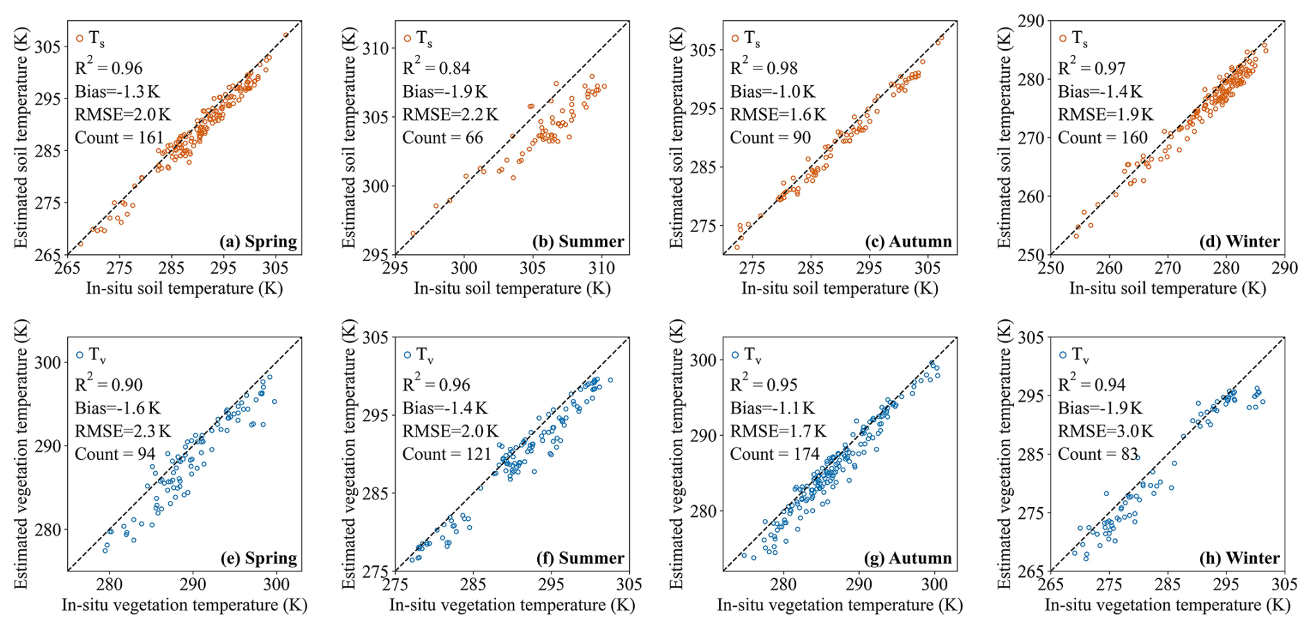
Figure 3 Validation of GloSVeT against in situ measurements across different seasons. Panels (a)–(d) show soil temperature (T_s), and panels (e)–(h) show vegetation temperature (T_v). The dashed line represents the 1:1 reference line. The Count value in each panel denotes the number of matched site-month records, and the corresponding numbers of independent sites for panels (a)–(h) are 14, 5, 12, 16, 16, 13, 20, and 15, respectively.

Seasonal variations in accuracy are evident. For soil temperature, performance was slightly lower in summer (R²=0.84, RMSE=2.2 K), likely due to the weaker constraint on the soil component under dense vegetation cover (Liu et al., 2020b; Zhan et al., 2011, 2013). In contrast, vegetation temperature retrievals showed larger errors in winter (RMSE=3.0 K), which may be attributed to the reduced contribution of the vegetation component to the mixed-pixel thermal signal under sparse canopy conditions. The highest agreement occurred in autumn for both components, when vegetation and atmospheric conditions were relatively stable, resulting in minimal uncertainty during component separation. In addition, it should be noted that the seasonal amplitude of vegetation temperature was less pronounced than that of soil temperature. Further examination shows that the soil temperature validation records were almost entirely from mid-latitude sites in all seasons, with 159/161, 66/66, 86/90, and 158/160 records in spring, summer, autumn, and winter, respectively. By contrast, the vegetation temperature validation records included a relatively high proportion of low-latitude samples, with 33/94, 37/121, 27/174, and 37/83 records in the four seasons, respectively. Because vegetation temperature in low-latitude regions generally has weaker seasonal variability and may remain relatively high even in winter, it is reasonable that the seasonal amplitude and magnitude range of vegetation temperature were less distinct than those of soil temperature in the validation samples.

Overall, these results indicate that GloSVeT achieves consistent and physically reasonable performance across seasons, with strong correlations (R²≥0.9 in most cases) and RMSE values generally around 2 K except for the larger winter error in vegetation temperature, effectively reproducing surface component temperatures at the monthly scale.

4.3 TC-based uncertainty evaluation

Figure 4 shows the results of the TC-based correlation (R) for soil temperature. In general, the three products exhibit largely consistent spatial patterns (Fig. 4a–c) and latitudinal variation (Fig. 4d). High correlations (R>0.7) are found mainly in the Northern Hemisphere high latitudes and the humid tropics, whereas low correlations (R<0.5) appear in many mid-latitude transitional regions. This spatial coherence across independent datasets indicates that the major large-scale thermal variations are consistently captured among the different data sources, and further supports the physical plausibility of the GloSVeT retrievals.

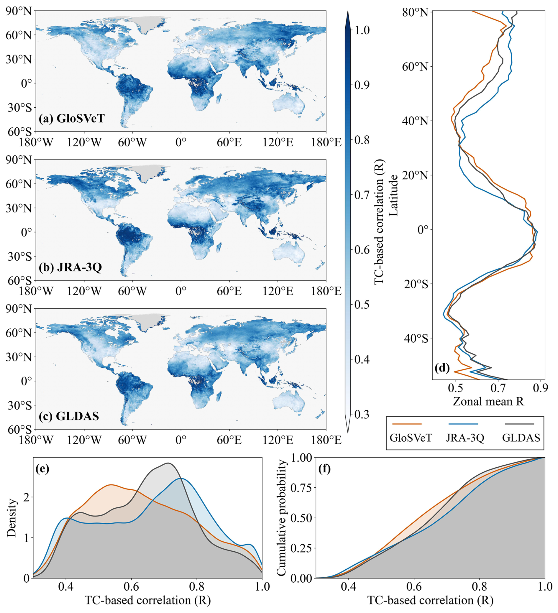
Figure 4 TC-based correlation (R) for soil temperature. Panels (a)–(c) illustrate the spatial distributions for GloSVeT, JRA-3Q, and GLDAS, respectively, with light gray and medium gray indicating the ocean and land backgrounds; (d) shows the zonal-mean R as a function of latitude; and panels (e) and (f) present the probability density and cumulative distribution functions, respectively.

Although their patterns are broadly similar, some differences can be observed among the three datasets. Overall, the inter-product differences are more evident in the Northern Hemisphere than in the Southern Hemisphere (Fig. 4d). JRA-3Q shows the highest correlations over regions north of 30° N, but shows the weakest performance across much of the remaining areas, particularly in tropical regions between 10 and 30° N (Fig. 4d). Its distribution contains a larger share of both very high (R>0.8) and very low (R<0.4) correlations (Fig. 4e and f), reflecting spatial heterogeneity and less stable behaviour at global scale. In contrast, GLDAS and GloSVeT achieve more equivalent performance (Fig. 4e and f). GLDAS shows a distribution concentrated around moderate-to-high R values (R between 0.6 and 0.8), whereas GloSVeT presents a smoother distribution and maintains more concentrated distribution toward higher R values (Fig. 4a and e). In particular, GloSVeT shows locally higher or comparable R values in humid tropical and subtropical regions, such as southern China, the Amazon and the Congo Basin, underscoring its advantage in these environmentally sensitive and data-scarce areas. By contrast, its correlations are lower at high latitudes. This may occur because JRA-3Q and GLDAS represent layer-averaged subsurface soil temperatures, whereas GloSVeT soil temperature represents the radiometric temperature of the visible surface and is more sensitive to snow cover and radiative inversions (Cao et al., 2023; Liu et al., 2025). Taken together, the TC-based evaluation suggests that reanalyses perform better in high latitude regions, whereas GloSVeT shows a relatively more balanced performance across latitudes and retains certain advantages in humid tropical regions. These results indicate that GloSVeT provides reliable surface soil temperature estimates and serves as a useful complement to conventional reanalysis soil temperature products for large-scale applications.

To extend the assessment from a global view to ecosystem contexts, this study further compared TC-based correlations for soil temperature across 14 biome types (Fig. 5). In general, the three datasets show higher median correlations (R≈0.7–0.9) in cold high-latitude and humid tropical ecosystems, such as temperate coniferous and mixed forests, boreal forests, tundra (Fig. 5e, f, and k), and tropical moist broadleaf forests and mangroves (Fig. 5a and n). In contrast, lower correlations (R≈0.5) with larger spreads are observed in Mediterranean, arid, and temperate grassland systems (Fig. 5l, m, and h). This cross-biome consistency reinforces that large-scale soil thermal variations are physically coherent across independent datasets.

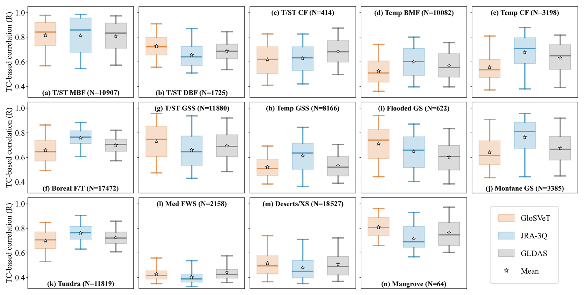
Figure 5 TC-based correlation (R) for soil temperature across 14 major biomes. Boxplots show the distributions of R for GloSVeT (orange), JRA-3Q (blue), and GLDAS (dark gray). Stars denote the mean values. T/ST, MBF, DBF, CF, Temp, BMF, F/T, GSS, GS, Med, FWS, and XS, are the abbreviations of “Tropical/subtropical”, “moist broadleaf forests”, “dry broadleaf forests”, “coniferous forests”, “Temperate”, “broadleaf and mixed forests”, “forests/taiga”, “grasslands, savannas and shrublands”, “grasslands and savannas”, “Mediterranean”, “forests, woodlands and scrub or sclerophyll forests”, and “xeric shrublands”, respectively.

Among the three products, JRA-3Q shows the largest inter-biome variability. It performs best in cold and mid-latitude forest ecosystems, such as boreal forests, tundra, montane grasslands, and temperate mixed or coniferous forests (Fig. 5f, k, j, d, and e), but its correlations drop markedly in tropical and semi-arid regions. Its boxplots also display wider interquartile ranges, indicating higher spatial heterogeneity and weaker internal consistency. By contrast, GloSVeT and GLDAS exhibit more comparable performance across most biomes. GLDAS generally shows moderate-to-high correlations, whereas GloSVeT maintains relatively balanced correlations across biome types and performs particularly well in tropical dry broadleaf forests, tropical/subtropical grasslands, savannas and shrublands, flooded grasslands, deserts/xeric shrublands, and Mangrove (Fig. 5b, g, i, m, and n), highlighting its ability to capture surface soil thermal variability under complex vegetation and moisture conditions. Overall, the biome-specific comparison supports the global results in Fig. 4, indicating that reanalysis products tend to perform better in cold and high-latitude ecosystems, whereas GloSVeT provides a relatively robust performance across diverse biome types with advantages in humid tropical and moisture-variable environments.

Figures 6 and 7 present the TC-based correlations for vegetation temperature. Since the analysis was restricted to densely vegetated pixels, and only pixels with more than 100 matched pairs were included to ensure the reliability of TC estimation, the resulting coverage was concentrated mainly over tropical and subtropical regions. Similar to the soil component, the three datasets display broadly consistent spatial and latitudinal patterns, yet GloSVeT systematically exhibits higher correlations and a narrower spread. As shown in Fig. 6a–d, across South America, Africa, and Southeast Asia, GloSVeT achieves stronger and more spatially uniform correlations (R>0.8) than JRA-3Q and GLDAS. The probability density and cumulative distribution curves (Fig. 6e and f) further indicate that GloSVeT contains a greater fraction of high R pixels and fewer low R outliers, reflecting improved temporal coherence and spatial stability. When compared across major vegetation types (Fig. 7), GloSVeT shows the highest or comparable median correlations in tropical/subtropical moist broadleaf forests, tropical/subtropical dry broadleaf forests, and temperate broadleaf and mixed forests (Fig. 7a–c). In tropical/subtropical grasslands, JRA-3Q exhibits slightly higher median correlations, but GloSVeT remains close to JRA-3Q and clearly higher than GLDAS (Fig. 7d). These results underscore the superior performance of GloSVeT in representing canopy thermal dynamics across diverse hydroclimatic conditions.

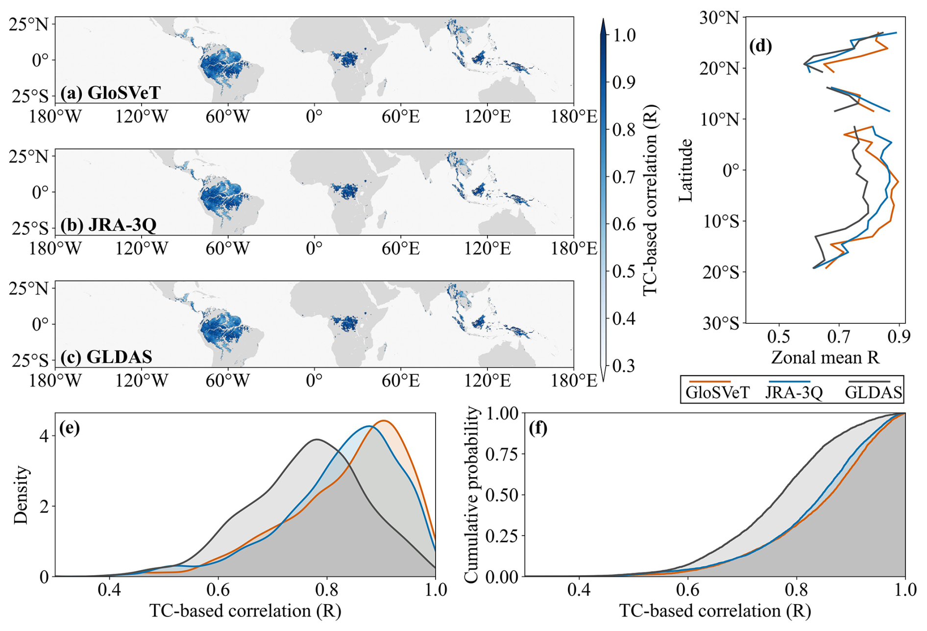
Figure 6 TC-based correlation (R) for vegetation temperature. Panels (a)–(c) illustrate the spatial distributions for GloSVeT, JRA-3Q, and GLDAS, respectively, with light gray and medium gray indicating the ocean and land backgrounds; (d) shows the zonal-mean R as a function of latitude; and panels (e) and (f) present the probability density and cumulative distribution functions, respectively.

Figure 7 TC-based correlation (R) for vegetation temperature across four major biomes. Boxplots show the distributions of R for GloSVeT (orange), JRA-3Q (blue), and GLDAS (dark gray). Stars denote the mean values. T/ST, MBF, DBF, Temp, BMF, and GSS, are the abbreviations of “Tropical/subtropical”, “moist broadleaf forests”, “dry broadleaf forests”, “Temperate”, “broadleaf and mixed forests”, and “grasslands, savannas and shrublands”, respectively.

4.4 Physical consistency assessment

Figure 8 illustrates the correlation between GloSVeT soil temperature anomalies and ESA CCI soil moisture anomalies for the best lag. At the global scale (Fig. 8a), negative correlations dominate the selected results (77.6 %; blue shading), indicating that wetter soil conditions are generally associated with lower soil temperatures. This spatially pervasive inverse relationship reflects the fundamental energy partitioning mechanism, where increased soil moisture enhances latent heat flux at the expense of sensible heating, leading to surface cooling. This mechanism has been well documented in both modeling and satellite-based studies (Benson and Dirmeyer, 2021; Gurung and Chen, 2024; Seneviratne et al., 2010). In contrast, positive correlations (22.4 %; red shading) are also evident in several dryland regions, particularly across the Sahara, West and Central Asia, and northwestern China, as well as in parts of high latitude and coastal areas, indicating that the soil temperature and soil moisture relationship is not uniformly characterized by evaporative cooling. In cold regions, these positive associations may be related to snowmelt, freeze thaw transitions, and snow insulation effects, through which warmer ground conditions can coincide with increases in liquid soil moisture (Hu et al., 2006; Jiang et al., 2023). In arid and semi-arid regions, where persistent evaporative cooling is often constrained by limited water availability, positive correlations may reflect episodic rainfall, irrigation, or warm season wetting events (Kong and Huber, 2023; Manzoni et al., 2020). In coastal and wetland environments, hydrological regulation, inundation, and coupled water and energy dynamics may further complicate the soil temperature and soil moisture relationship (Yu et al., 2024).

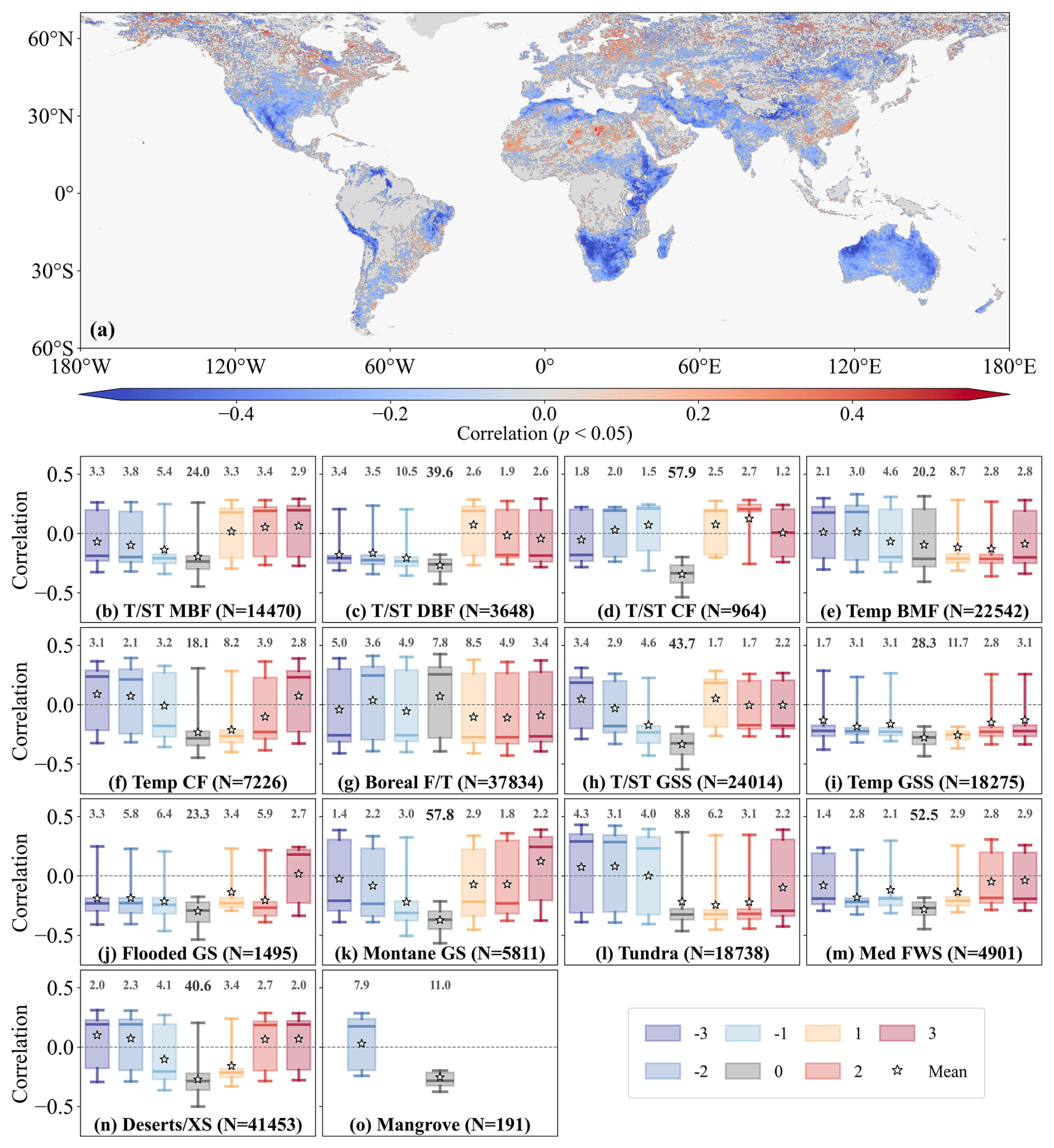
Figure 8 Correlation between GloSVeT soil temperature anomalies and ESA CCI soil moisture anomalies for the best lag. Panel (a) shows the spatial distribution of correlations for pixels with an identified best lag, where red and blue indicate positive and negative relationships, respectively. Panels (b)–(o) present the distributions of these correlations across 14 major biomes. Boxplots with different colors denote the identified lag months from −3 to +3. The numbers above each box indicate the percentage of pixels assigned to each identified lag month within the corresponding biome, with darker colors and larger font sizes representing higher proportions. N denotes the total number of pixels in each biome category.

Across biome types (Fig. 8b–o), the proportion of pixels with an identified best lag and the corresponding strength of soil temperature–moisture correlations exhibit distinct ecological patterns. Overall, the fraction of significant correlations is highest in montane grasslands (71.3 %) and tropical/subtropical coniferous forests (69.5 %), followed by Mediterranean woodlands (67.4 %), tropical dry broadleaf forests (64.1 %), and tropical/subtropical grasslands and savannas (60.1 %). Intermediate proportions (≈50 %–55 %) are observed in temperate grasslands and flooded grasslands, whereas high-latitude biomes such as boreal forests (38.0 %) and tundra (31.7 %) show much lower ratios. Mangroves have the lowest value (18.8 %), likely due to their limited spatial extent and the strong influence of coastal hydrodynamics. This spatial gradient suggests that in topographically complex or hydrothermally contrasting mid- and low-latitude systems, soil moisture exerts a more coherent and consistent control on soil temperature (Seneviratne et al., 2010; Williams et al., 2009), while in cold regions the coupling is weakened by snow, permafrost, and heterogeneous freeze–thaw processes (Zhao et al., 2022).

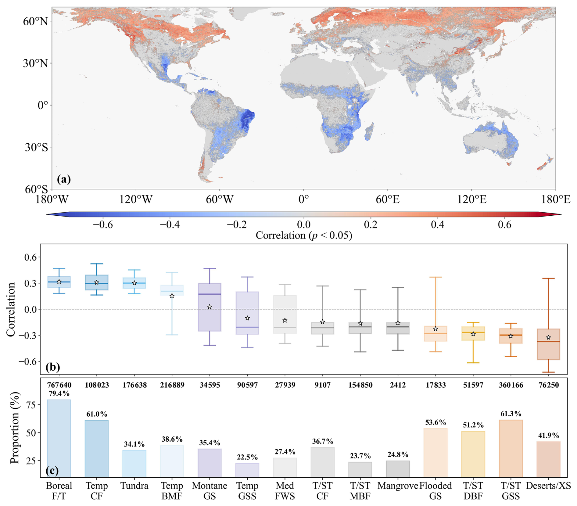
Figure 9 Correlation between GloSVeT vegetation temperature anomalies and GOSIF SIF anomalies. Panel (a) shows the spatial distribution of significant correlations (p<0.05), where red and blue indicate positive and negative relationships, respectively. Panel (b) presents the distribution of significant correlations across 14 major biomes. Panel (c) summarizes the proportion of significant pixels within each biome. In panel (c), the numbers above the bars indicate the total number of pixels in each biome category, and the percentages indicate the corresponding proportion of significant pixels.

Regarding correlation strength and lag dependence, Fig. 8 reveals a clear hierarchy in the soil temperature and soil moisture association. The dominant pattern is the prevalence of 0 month lags. In several mid and low latitude biomes, such as tropical seasonal forests and savannas, montane grasslands, Mediterranean shrublands, and arid ecosystems (Fig. 8c, d, h, k, m, and n), 0 month lags account for approximately 40 %–60 % of the pixels. A weaker but still evident 0 month dominance is also found in humid tropical forests, temperate forests and grasslands, and flooded grasslands (Fig. 8b, e, f, i, and j), where the 0 month lag remains the largest category but accounts for about 20 %–30 % of the pixels. These patterns indicate that the strongest monthly association between soil temperature and soil moisture anomalies most commonly occurs within the same month. Together with the generally negative median correlations and relatively compact spreads, this synchronous dominance is consistent with contemporaneous energy and water partitioning between soil moisture and surface thermal conditions. Beyond this overall synchronous pattern, nonzero lags reveal biome dependent differences in temporal ordering. In tropical and wetland related ecosystems, including tropical broadleaf forests, tropical savannas, and flooded grasslands (Fig. 8b, c, h, and j), negative lags are relatively more frequent than positive lags of the same length. This pattern indicates that soil moisture anomalies tend to precede soil temperature anomalies in part of these regions, suggesting that antecedent moisture conditions may remain linked to the subsequent monthly soil thermal state through soil water memory and rainfall driven drying and rewetting dynamics (Manzoni et al., 2020). In contrast, temperate and high latitude biomes, including temperate forests and grasslands, boreal forests, and tundra (Fig. 8e, f, g, i, and l), show relatively higher proportions of positive lags, indicating that soil temperature anomalies more often precede soil moisture anomalies. This temperature leading association may be related to cold season thermal transitions, during which seasonal snow cover and snow insulation strongly modulate ground surface temperature and complicate its monthly relationship with soil moisture (Cao et al., 2023). Collectively, these biome specific patterns suggest that GloSVeT soil temperature anomalies are linked to independent soil moisture anomalies through a physically interpretable temporal structure, characterized by dominant synchronous coupling, more evident moisture leading associations in tropical and wetland related ecosystems, and more evident temperature leading associations in temperate and high latitude regions. These results further support the physical consistency of GloSVeT in representing soil hydrothermal variability across diverse climatic regimes.

At the growing season scale, the relationship between GloSVeT vegetation temperature and SIF (Fig. 9) exhibits clear large-scale regularities. As shown in Fig. 9a, significant negative correlations dominate much of the subtropics and monsoon margins where soil moisture fluctuates strongly, indicating that warmer-than-normal canopies coincide with reduced photosynthetic activity. In contrast, positive correlations emerge mainly in energy-limited high latitude regions, where warmer growing season canopy conditions may bring vegetation closer to its photosynthetic thermal optimum and coincide with stronger physiological activity. These contrasting patterns align well with the classical framework of water versus energy limited canopy functioning (Alkama and Cescatti, 2016).

Regarding different biome types (Fig. 9b and c), the correlation strength follows a distinct gradient from cold and energy limited regimes to warm and water limited regimes. Boreal and temperate coniferous forests show the strongest positive correlations (∼0.3) with compact distributions and high fractions of significant pixels (79.4 % and 61.0 %), indicating that warmer vegetation conditions during the growing season are associated with higher SIF in ecosystems where low temperature or limited energy supply can constrain photosynthetic activity (Pan et al., 2024). Tundra exhibits similarly positive but less consistent correlations (34.1 %), as snow and permafrost may dampen the thermal–photosynthetic response. Transitional systems such as montane grasslands, temperate grasslands, and mangrove have around near-zero medians (absolute value <0.2) with broad variability and limited significance (<30 %), reflecting mixed thermal, moisture, and hydrological controls on vegetation activity. The strongest negative couplings occur in flooded grasslands, tropical/subtropical dry broadleaf forests, tropical/subtropical grasslands–savannas, and deserts/xeric shrublands (median $\sim -\mathrm{0.3}$ to −0.4), where canopy warming accompanies photosynthetic downregulation associated with water stress and stomatal closure (Doughty et al., 2023). Among these, tropical/subtropical savannas and dry forests show the most coherent relationships, while flooded and arid systems exhibit more dispersed patterns due to hydrological and edaphic heterogeneity. Collectively, these findings demonstrate that GloSVeT captures a biome dependent continuum between canopy thermal dynamics and photosynthetic activity.

4.5 Spatiotemporal variability and trends

A unique advantage of the GloSVeT dataset is that it provides soil and vegetation temperatures simultaneously, enabling consistent evaluation of their co-variability and long-term evolution. Figure 10 illustrates the temporal trends of globally averaged component temperatures for the pixels where both soil temperature and vegetation temperature are available. These two time series exhibit highly synchronous variations across sub-seasonal to interannual scales, with peaks and troughs closely aligned, indicating that soil and vegetation temperature changes are dynamically coupled. In terms of long-term trends, both components show pronounced warming over 2003–2023, with slopes of 0.44 ± 0.04 K per decade for soil temperature and 0.39 ± 0.04 K per decade for vegetation temperature (both p<0.001), suggesting slightly faster warming in the soil layer than in the canopy (García-García et al., 2023; Trew et al., 2024). The number of valid pixels ranges from 4.6×10⁶ to 5.2×10⁶, with a mean of 5.0×10⁶ and a standard deviation of 0.1×10⁶, confirming that the trend analysis is based on a stable and representative sample. The pixel count also exhibits a clear seasonal pattern, i.e., higher from June to October and lower in other months, which is consistent with vegetation growth cycles. All of these features highlight the robustness and physical consistency of the GloSVeT-derived temporal analysis.

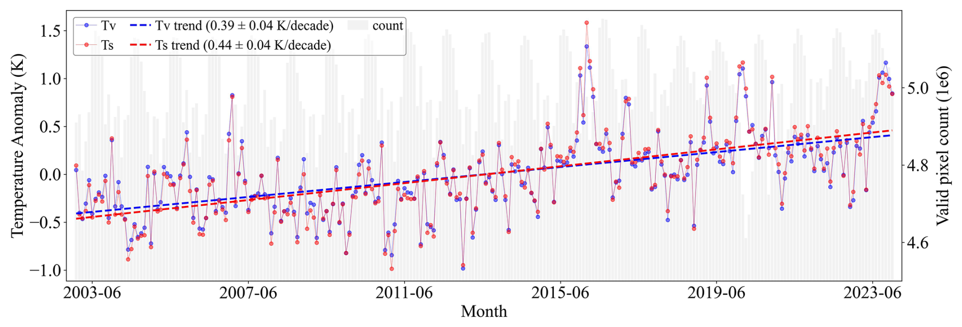
Figure 10 Global monthly anomalies of soil (T_s, red) and vegetation (T_v, blue) temperatures from 2003–2023. Dots show monthly means, dashed lines indicate linear trends, and grey bars (right axis) denote the number of valid pixels used each month.

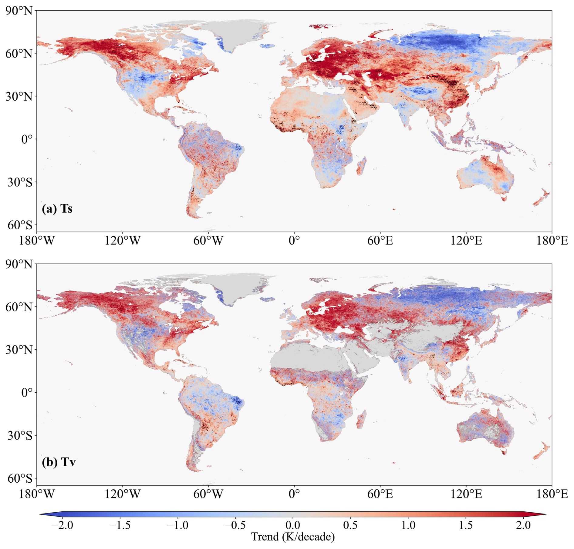
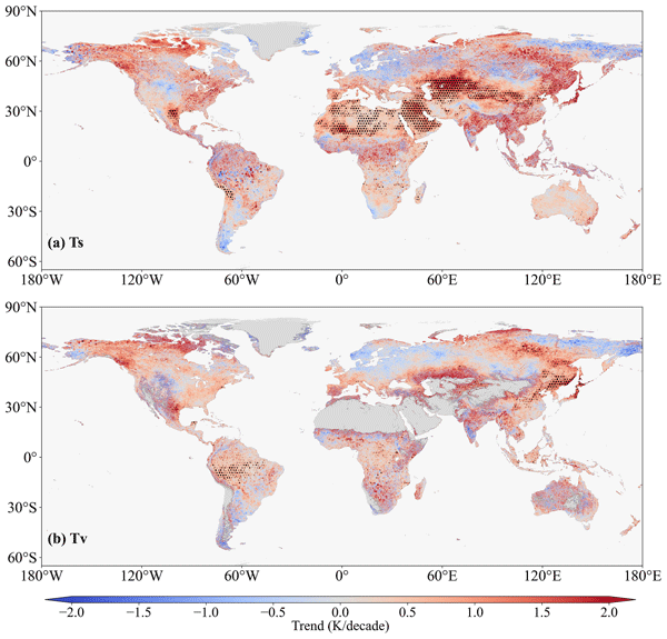
Figure 11 Linear trends of GloSVeT component temperatures in January for (a) soil and (b) vegetation during 2003–2023. Black dots indicate pixels with statistically significant trends (p<0.05).

To further investigate the spatial heterogeneity of these temporal trends, the linear slopes were mapped for representative cold (January) and warm (July) months (Figs. 11 and 12). In January, the majority of pixels showed positive trends, accounting for 68.4 % of soil temperature pixels and 62.3 % of vegetation temperature pixels, indicating a widespread tendency toward wintertime warming. Pronounced warming occurs across North America, Europe, and southeastern China, whereas localized cooling is evident in northern Eurasia and the high Asian interior (Bartusek et al., 2022; Qiao et al., 2025). However, only 6.7 % of soil temperature pixels and 7.0 % of vegetation temperature pixels passed the 0.05 significance test. These significant pixels were not randomly distributed, but were mainly concentrated in regions with relatively strong warming or cooling signals, indicating that the most pronounced trend centres are more statistically robust. The large fraction of non-significant pixels is likely related to the limited number of annual samples for each calendar month (21 values during 2003–2023) and strong interannual variability. Therefore, the non-significant regions should be interpreted as areas with weak or uncertain pixel-level trends, rather than as evidence of no thermal change. Compared with soil temperature, vegetation trends are generally weaker, consistent with the effects of snow masking, stronger canopy–air coupling during cold seasons, and the thermal buffering imposed by canopy structure and aerodynamic resistance (Forzieri et al., 2017). In the Southern Hemisphere, January trends are weaker and more heterogeneous, reflecting the smaller land area, weaker continental thermal contrast, and stronger oceanic modulation during austral summer. In July, warming becomes more spatially extensive covering 74.8 % of soil temperature and 70.7 % of vegetation temperature pixels, but the overall rate is slightly lower. Broad warming is observed across the Northern Hemisphere mid-latitudes, particularly in western North America, the Mediterranean–Middle East, Central Asia, and northeastern China, whereas parts of Europe display moderate cooling. The proportion of statistically significant pixels increased in July, reaching 16.6 % for soil temperature and 10.8 % for vegetation temperature, indicating a stronger and more spatially coherent warm-season trend signal than in January. Consistent with the cold-season behaviour, soil temperature trends exceed those of vegetation temperature, reflecting the greater sensitivity of the soil skin to net radiation and the reduced evaporative buffering from vegetation (Qiao et al., 2023). In summary, these distinct seasonal behaviours, including stronger winter contrasts at high latitudes and widespread summer warming over continental interiors, suggest that GloSVeT captures meaningful large-scale structures of surface thermal change, while pixel-level interpretations in non-significant regions should be made with caution.

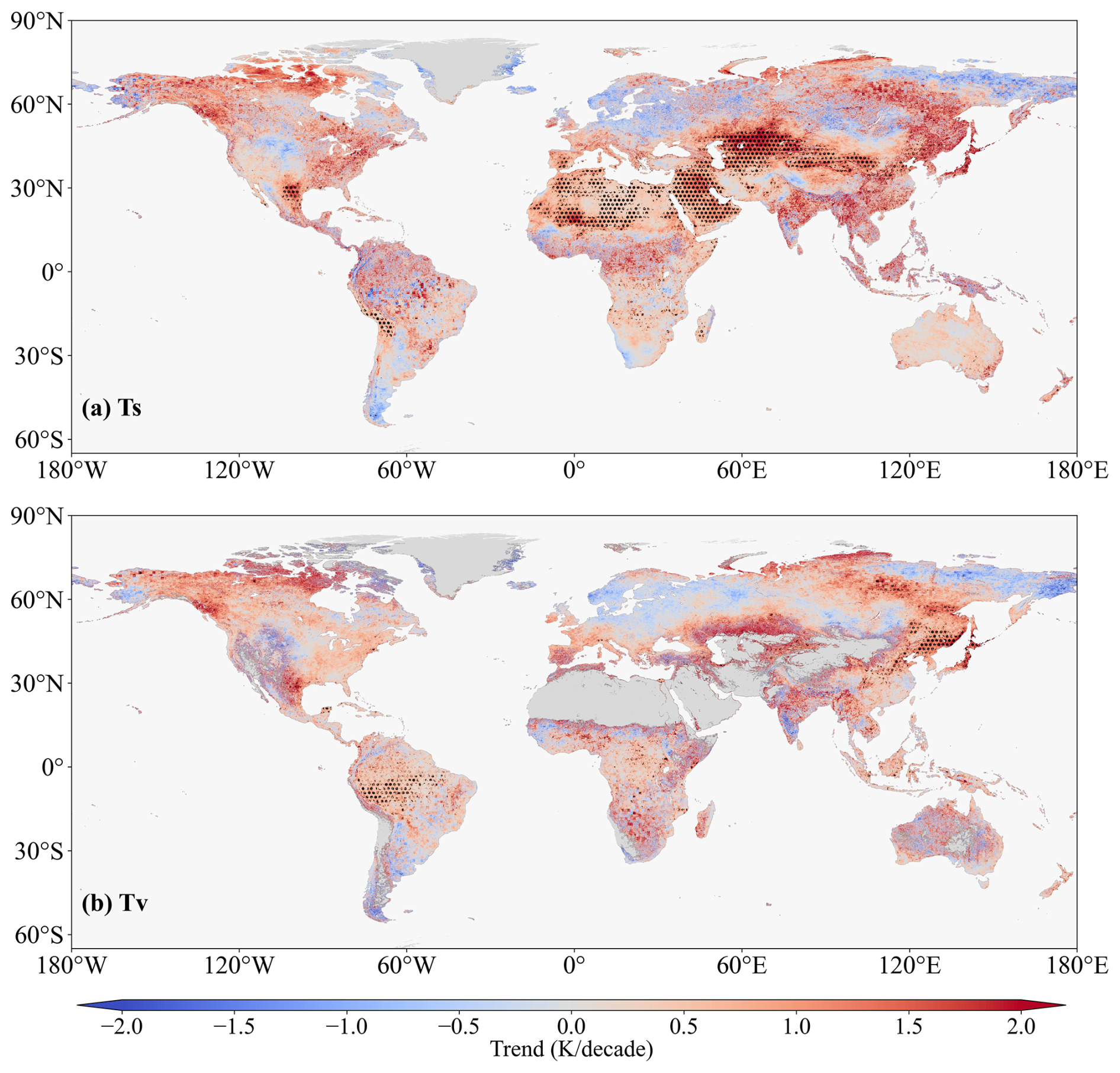
Figure 12 Linear trends of GloSVeT component temperatures in July for (a) soil and (b) vegetation during 2003–2023. Black dots indicate pixels with statistically significant trends (p<0.05).

5 Discussion

5.1 Influence of fixed emissivity

In GloSVeT, the broadband emissivities of soil and vegetation were uniformly set to 0.95 and 0.98, respectively. For a global product, such fixed emissivity assumptions inevitably introduce uncertainty, particularly for soil component (García-Santos et al., 2015). Therefore, we conducted an emissivity sensitivity analysis to evaluate the potential influence of this assumption on the retrieved soil and vegetation component temperatures. Specifically, nine soil–vegetation emissivity combinations were tested, with soil emissivity set to 0.90, 0.93, and 0.95, and vegetation emissivity set to 0.97, 0.98, and 0.99. Based on the 12 monthly datasets in 2023, the global valid pixels were stratified into FVC bins at an interval of 0.1, and 1000 valid samples were randomly selected from each FVC bin for each month. Soil and vegetation component temperatures were then recalculated under each emissivity combination. Taking the baseline setting used in GloSVeT (ε_s=0.95 and ε_v=0.98) as the reference, the mean absolute error (MAE) induced by the other eight emissivity perturbation scenarios was calculated.

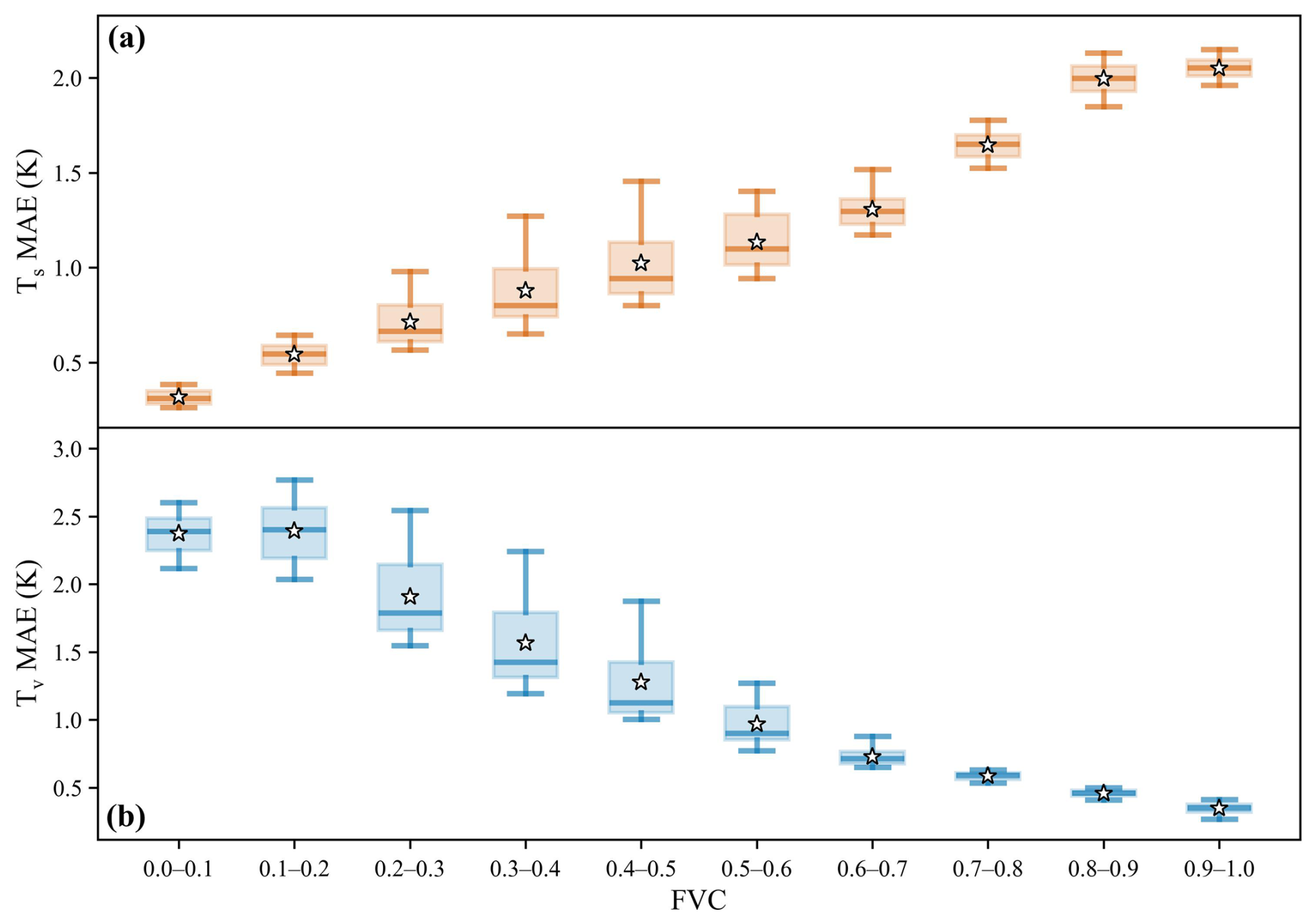
Figure 13 Sensitivity of GloSVeT to emissivity perturbations across FVC gradients for soil temperature (a) and vegetation temperature (b). Boxplots summarize the MAE distributions derived from 12 monthly datasets in 2023 and eight emissivity perturbation scenarios relative to the baseline emissivity setting used in GloSVeT.

Figure 13 presents the distribution of MAE across FVC bins, where each boxplot contains 96 MAE statistics derived from 12 months and 8 emissivity perturbation scenarios. The results reveal that sensitivity to emissivity assumptions is strongly dependent on FVC: as FVC increases, the emissivity sensitivity of soil component temperature gradually increases, whereas that of vegetation component temperature decreases. Without separating FVC conditions, the median MAEs of T_s and T_v are 1.16 and 1.26 K, respectively, suggesting that the overall influence of the fixed emissivity assumption remains within a relatively limited range. A more detailed FVC-dependent analysis further indicates that emissivity uncertainty has a smaller impact on the dominant component within a mixed pixel. When FVC is below 0.5, the soil component dominates the mixed-pixel thermal signal, and the MAE of T_s is generally below 1 K. Conversely, when FVC exceeds 0.5, the vegetation component is more strongly constrained, and the MAE of T_v is typically below 1 K. In contrast, under very low or very high FVC conditions, the weakly represented component contributes less to the mixed-pixel thermal signal and therefore becomes more sensitive to emissivity perturbations. Therefore, the fixed emissivity assumption does not substantially weaken the overall ability of GloSVeT to represent the dominant component temperature, but the non-dominant component temperature under extreme FVC conditions should be interpreted with caution.

5.2 Application potential

Based on extensive validation and consistency assessments, the GloSVeT dataset demonstrates reliable accuracy and strong physical consistency, offering broad potential for applications in land–atmosphere interaction studies, ecosystem monitoring, and model integration. First, by explicitly resolving the thermal contrast between soil and vegetation, GloSVeT facilitates the separation of energy partitioning between soil evaporation and vegetation transpiration under varying vegetation covers. This capability is valuable for diagnosing surface–atmosphere coupling strength and improving the parameterization of energy balance models from regional to global scales (Li et al., 2023; Song et al., 2020). Second, the vegetation–soil temperature difference (ΔT) derived from GloSVeT is a physically based indicator that shows higher sensitivity to evaporative stress and canopy water deficit than the traditional canopy–air temperature difference (Luan and Vico, 2021). By linking ΔT dynamics with soil moisture and vegetation optical indices, GloSVeT enables consistent detection of ecosystem drought responses and recovery trajectories across climatic gradients. Third, through the retrieval of spatially explicit and physically consistent vegetation temperatures, GloSVeT establishes key biophysical constraints for simulating crop productivity and terrestrial carbon exchange. Consequently, it can act as a robust alternative to conventional LST for coupling with photosynthetic metrics such as GPP to diagnose thermal stress impacts on crop performance and vegetation carbon assimilation (Prentice et al., 2024). Finally, owing to its global coverage, multi-decade record, and physically interpretable design, GloSVeT constitutes a valuable forcing or evaluation dataset for land surface and biogeochemical models. For instance, it can be incorporated into or benchmarked within modeling frameworks to improve the representation of surface thermal inertia, soil–canopy coupling, and energy–carbon feedbacks.

5.3 Limitations

Despite the broad application potential of GloSVeT, its physical meaning and applicability need to be clearly defined. First, the soil and vegetation temperatures in GloSVeT are separated from TIR LST, and represent the radiative thermal states of the visible surfaces within the sensor field of view. Therefore, under dense canopy or seasonal snow cover conditions, the retrieved soil temperature does not necessarily correspond to the actual soil temperature beneath the canopy or snowpack. Second, the current two-component framework approximates the land surface as a combination of vegetation and soil components. However, over complex surfaces such as urban or mountainous regions, the so-called soil component temperature may include impervious surfaces, exposed rocks, or other non-vegetation materials, and should therefore be interpreted as a non-vegetation background component temperature in these areas. This simplification also does not explicitly distinguish between sunlit and shaded fractions. Temperature differences among vegetation, sunlit soil, and shaded soil can be substantial and represent an important source of thermal radiation directionality (Ermida et al., 2014; Liu et al., 2020a; Qin et al., 2025; Lu et al., 2025). As a result, the conventional two-component framework adopted in GloSVeT may overlook sub-pixel thermal heterogeneity, especially for the soil component. Finally, TIR observations correspond to the thermal state of a very shallow layer, typically on the order of 1–100 µm (Li et al., 2023), rather than the soil thermal state at a certain depth or the complete three dimensional thermal state inside the canopy. Consequently, GloSVeT is more suitable for characterizing the surface radiative thermal states of visible soil/background and vegetation components. For applications involving under-canopy soil temperature, sub-snow soil temperature, urban background thermal states, or vertical heat transfer processes, GloSVeT should be interpreted cautiously in combination with land cover, snow cover, topographic, or canopy structural information. Future developments could further integrate more detailed surface component structure information, soil heat diffusion models, and canopy energy transfer models to extend GloSVeT surface component temperatures toward more explicit vertical soil and canopy thermal states (Cao et al., 2023; Lundquist et al., 2018).

A second limitation arises from the clear-sky nature of TIR satellite observations and uncertainties in related input data. The MODIS LST observations used in GloSVeT are available only under clear-sky conditions, whereas the intended monthly mean component temperatures are expected to represent the average thermal state under all-weather conditions within each month. Although ERA5-Land provides continuous all-sky diurnal thermal information and helps constrain the monthly mean diurnal cycle, the retrieved component temperatures are still ultimately constrained by clear-sky TIR observations. This mismatch between clear-sky observation and the all-weather monthly mean target may introduce sampling biases, especially in persistently cloudy regions or during periods when cloudy-sky and clear-sky surface thermal conditions differ systematically. Such uncertainty could be reduced by incorporating cloud-contaminated LST reconstruction algorithms (Jia et al., 2024; Du et al., 2025) or by directly using advanced all-weather LST products. For example, GHA-LST (Jia et al., 2023), a global, hourly, 5 km, and all-weather LST dataset, provides a promising data source for improving the temporal completeness and all-weather representativeness of component temperature retrievals. A related input data issue is the orbital drift of the Terra and Aqua satellites during the later MODIS period, especially after 2021, which may introduce temporal sampling uncertainty because the actual overpass times deviate from the nominal MODIS overpass times. Although this effect is partly mitigated by monthly scale processing and the use of ERA5-Land diurnal cycle information, it may still influence the results toward the end of the data record. This issue could be further addressed by incorporating orbit drift correction (Julien and Sobrino, 2025; Liu et al., 2019) or by introducing additional sensors, such as VIIRS, within the FuSVeT framework.

The validation strategy also has inherent limitations. Although the TC analysis provides an effective way to evaluate GloSVeT in the absence of globally available long-term observations of soil and vegetation temperatures, its results should be interpreted within the context of proxy-based comparison. The reanalysis soil temperatures used in TC represent near-surface soil thermal states at specific depths, which are physically related to but not identical to the TIR-constrained surface radiometric temperature retrieved by GloSVeT (Cao et al., 2023; Liu et al., 2025). Similarly, near-surface air temperature was used as an auxiliary proxy for vegetation temperature in densely vegetated regions (Li et al., 2001; Zhan et al., 2011; Rutter et al., 2023), but it is not equivalent to vegetation temperature. Therefore, the TC-based correlations mainly indicate the relative temporal consistency between GloSVeT and physically related independent datasets, rather than absolute accuracy against true soil or vegetation component temperatures. More direct and spatially representative observations of surface soil and vegetation temperatures would help further strengthen the independent validation of GloSVeT and reduce the uncertainty associated with proxy-based comparisons.

Finally, GloSVeT relies on the GOT09-based MDC model, which assumes a relatively regular diurnal temperature cycle characterized by daytime warming and nighttime cooling. This assumption can be weakened or violated in high-latitude regions during polar day and polar night, when the conventional diurnal heating and cooling cycle becomes weak or absent (Hong et al., 2018). Under such conditions, GloSVeT retrievals may have larger uncertainties and therefore require cautious interpretation. Further refinements to GloSVeT should consider diurnal temperature cycle formulations that are better suited to polar illumination conditions and irregular diurnal temperature cycles. In addition, GloSVeT is currently produced at a monthly temporal resolution and reports monthly mean surface component temperatures. This design reflects a balance among input data availability, computational efficiency, and the intended use of the dataset for climate scale analyses. However, monthly data cannot resolve short term thermal responses to rainfall, irrigation, soil water saturation, heatwaves, or rapid vegetation stress events. Extending GloSVeT to daily or sub monthly scales would increase its value for near-real-time monitoring and process level modeling, particularly for evaluating the immediate coupling between soil moisture and soil/background temperature (Li et al., 2022). Furthermore, the current product provides mean component temperatures, while other thermal metrics derived from diurnal temperature cycle models, such as diurnal range, maximum temperature, and minimum temperature, would better characterize thermal variability and climate extremes (Li et al., 2023; Liu et al., 2023; Zhao et al., 2025). These extensions would further improve the utility of GloSVeT for land surface modeling, agricultural monitoring, drought assessment, and ecosystem stress diagnosis.

6 Code and data availability

The global 0.05° monthly mean surface soil and vegetation component temperature dataset (GloSVeT) covering the period 2003–2023 is publicly available at https://doi.org/10.11888/RemoteSen.tpdc.303317 (Liu and Li, 2026a) and https://doi.org/10.5281/zenodo.22724289 (Liu and Li, 2026b). Data are provided as GeoTIFF files in UInt16 format with a scale factor of 0.02, expressed in Kelvin (K), and a fill value of 65 535. The current GloSVeT release does not include separate pixel-level quality control layers or recommended reliability flags. Users who need additional screening information can refer to the original input datasets, including the Clear_sky_days and Clear_sky_nights layers in MxD11C3 for clear-sky MODIS sampling, GLASS FVC for component dominance, and MCD12C1 land cover for identifying surface types that require cautious interpretation. The dataset can be directly accessed and used without any specialized software. The main code used for dataset generation, uncertainty evaluation, physical consistency validation, trend analysis, and figure reproduction is also available in the same Zenodo archive (Liu and Li, 2026b).

7 Conclusions

Using the FuSVeT method adapted for global implementation, this study produced the first global dataset of soil and vegetation component temperatures (GloSVeT), providing monthly means at 0.05° spatial resolution for 2003–2023. To ensure reliability, a comprehensive multi-perspective evaluation was performed, integrating internal closure check, flux-tower validation, triple collocation analysis, physical consistency assessment, and spatiotemporal trend examination. The internal closure check showed that GloSVeT can largely reproduce the original MODIS mixed-pixel LST signal, indicating that the component temperature separation remains consistent with the input radiometric constraint. Validation against flux-tower measurements demonstrated high accuracy for both components (R²≥0.9 and RMSE∼2 K in most cases), with a minor, physically interpretable cool bias linked to the diurnal sampling of satellite observations. The triple collocation analysis further confirmed strong temporal coherence and spatial robustness, showing globally consistent performance with strengths in humid tropics and transitional environments, while reanalysis products performed relatively better at high latitudes. Physical consistency assessments revealed clear process-based relationships: soil temperature anomalies were predominantly negatively correlated with soil moisture, consistent with evaporative cooling as the dominant pattern, whereas vegetation temperature exhibited biome-dependent coupling with SIF, transitioning from positive correlations in energy-limited regions to negative ones in water-limited ecosystems. Spatiotemporal analyses showed pronounced warming trends in both soil (0.44 ± 0.04 K per decade) and vegetation (0.39 ± 0.04 K per decade) components during 2003–2023, with seasonally interpretable patterns characterized by stronger winter contrasts at high latitudes and widespread summer warming over continental interiors. Collectively, these results demonstrate that GloSVeT achieves physically consistent, spatially coherent, and dynamically realistic performance across diverse climatic regimes. Therefore, this new dataset is expected to provide a valuable foundation for quantifying land–atmosphere energy exchange, monitoring ecosystem hydrothermal dynamics, and improving the representation of surface processes in Earth system models.

Appendix A: Supplementary tables and figures

Table A1 Summary of representative soil temperature products.

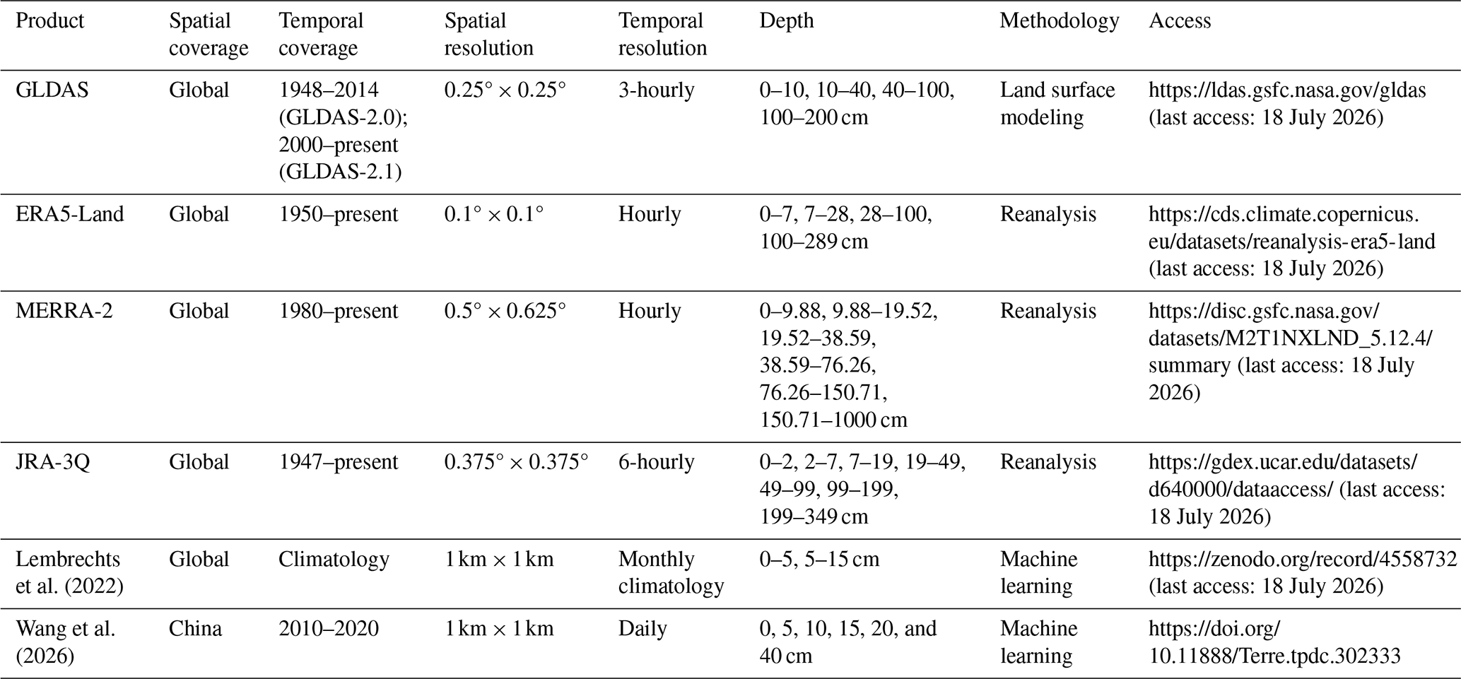
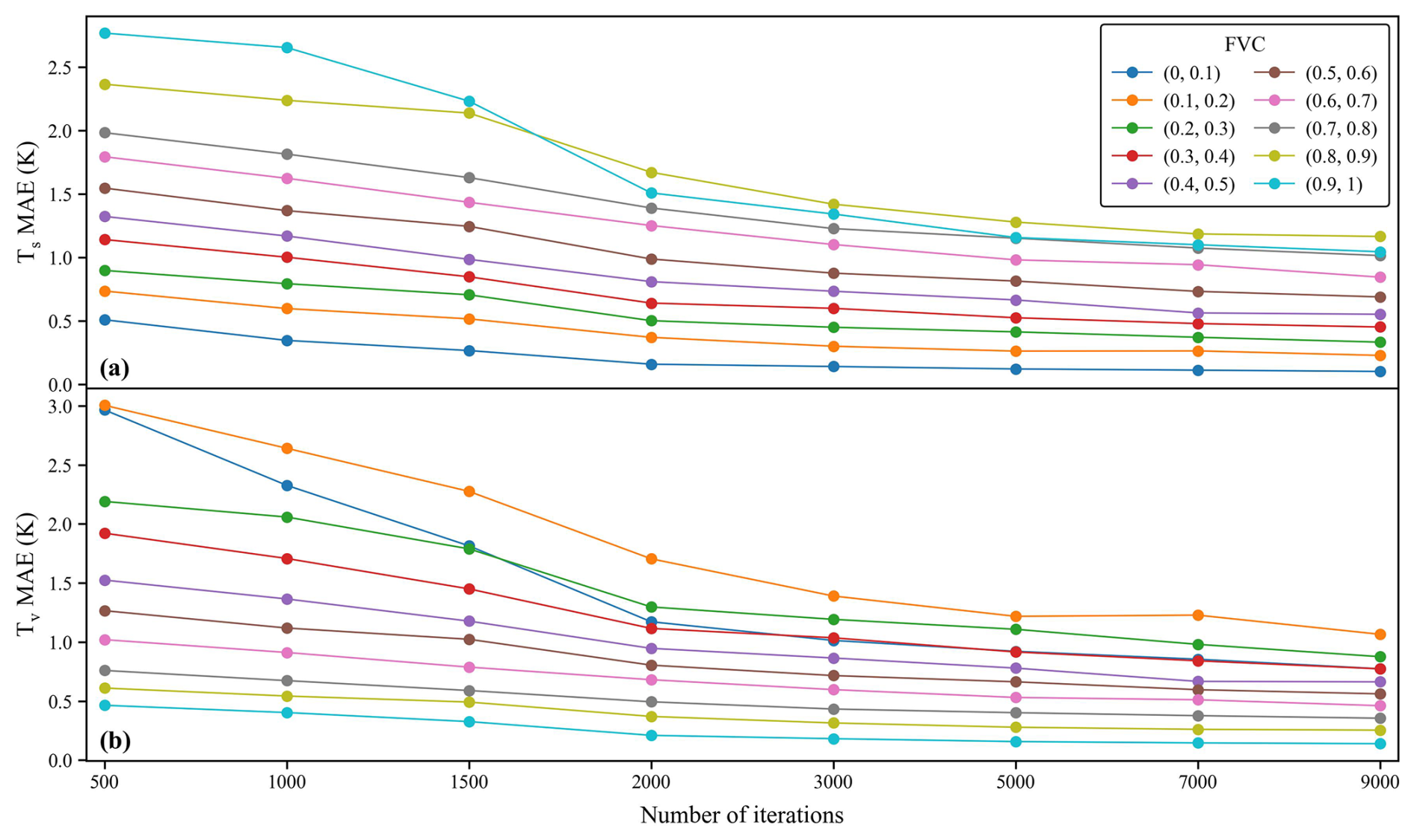
Figure A1 Convergence test of Bayesian optimization across FVC bins. Using the July 2023 data, valid pixels were stratified into ten FVC bins, and 1000 samples were randomly selected from each bin. Bayesian optimization was performed with 500, 1000, 1500, 2000, 3000, 5000, 7000, and 9000 iterations, and the result from 10 000 iterations was used as the reference solution. The MAE values of retrieved soil temperature (a) and vegetation temperature (b) were calculated relative to this reference solution. Different lines represent different FVC bins.