the Creative Commons Attribution 4.0 License.
the Creative Commons Attribution 4.0 License.
 | 01 Sep 2026
Global surface mining and land reclamation of time series from 1985–2022
Sucheng Xu
Jiatong Zhou
Kechao Wang
Stefan Giljum
Victor Maus
Tim T. Werner
Liang Tang
Jiwang Guo
Wu Xiao

Surface mining has profound impacts on ecosystems, contributing to land degradation, vegetation loss, pollution, and threats to biodiversity. Given the rapidly rising demand for raw materials, understanding the dynamics of mining and reclamation processes is essential to support sustainable development. Here, we integrate and analyze a large set of mines distributed worldwide based on their known land extent circa year 2020. We integrated time-series data of the Normalized Difference Vegetation Index (NDVI), nighttime light (NTL) intensity, and land use to detect and identify changes within mine sites from 1985 to 2022 and assess spatiotemporal trajectories of mining and reclamation processes. The dataset comprises 74 726 polygons, covering a total area of 82 552 km2. Our dataset obtained the maximum potential mining disturbance boundary – the cumulative outer envelope of mining-induced land disturbance over the study period. China leads in both the number and the areal extent of mining sites, followed by the United States and Australia. Within the analyzed set of polygons, mining land footprint expanded steadily between 1985 and 2022, with the annual disturbed area peaking at 1943 km2 in 2015, with a slowing expansion after 2015. From 1985 to 2022, the cumulative area of land converted to mine reached 40 596 km2, accounting for 49 % of the total surface mining area in our set, while the reclaimed area was 29 285 km2. Active mining areas dominated the global mining landscape, comprising 31.6 % of all polygons, with approximately 50.6 % concentrated in Asia. The spatiotemporal processes and patterns revealed in this study provide crucial insights into the development of mine sites and provide new data to support ecological impact assessments and sustainable development research in global mining regions. The dataset is available at Zenodo at https://doi.org/10.5281/zenodo.17085099 (Xu et al., 2025).
- Article
(15815 KB) - Full-text XML
- BibTeX
- EndNote


Mining activities are a fundamental driver of global economic growth and play a key role in industrial development (Pavloudakis et al., 2024). However, mining causes significant disruptions to ecosystems, particularly through vegetation loss, biodiversity decline, water pollution and ecological degradation (Chen et al., 2025b; Giam et al., 2018; Giljum et al., 2025; Qian et al., 2018; Xiang et al., 2021). Surface mining, involving extensive soil stripping and land excavation, alters the surface landscape, significantly modifies ecosystem structure and function, and causes habitat loss, which contributes to biodiversity decline (Firozjaei et al., 2021; Giljum et al., 2022; Ma et al., 2021; Xiao et al., 2020a; Yan et al., 2024; Zhao et al., 2023). Studies in tropical regions, for example, have shown that mining activities can cause deforestation within a 70 km radius, with indirect impact up to 28 times greater than direct impacts (Ladewig et al., 2024; Sonter et al., 2017). As global demand for mineral resources continues to grow, mining activities have expanded at an unprecedented rate. Global extraction of fossil fuels, metal ores, and non-metallic minerals increased from approximately 45.7 billion tonnes in 2004 to a projected 79.7 billion tonnes in 2024, representing an increase of approximately 75 % (Schandl et al., 2024). The International Energy Agency (IEA) estimates that achieving net-zero global greenhouse gas emissions by 2050 will require a sixfold increase in demand for key minerals, with some critical minerals, such as lithium, experiencing a 40-fold increase (Carr-Wilson et al., 2024). As the scale of mining inevitably expands globally, the need for monitoring and assessing its ecological impacts is becoming increasingly urgent. A systematic understanding and analysis of the precise spatial locations of global mining activities, the boundaries of mining-induced degradation, and reclamation processes form the foundation for assessing the ecological impacts of mining. However, impacts on more than half of the world's mining areas go unrecorded due to data limitations (Maus and Werner, 2024), severely limiting the precise assessment of mining's environmental impact and the exploration of sustainable development pathways.
Globally, research focused on delineating mining area boundaries and monitoring the spatiotemporal dynamics of vegetation disturbance and reclamation is steadily increasing (Werner et al., 2019). However, these studies still have considerable room for improvement, particularly regarding the number of mining sites, boundary accuracy, and monitoring methods for vegetation disturbance. In recent years, visual interpretation of satellite imagery has been applied to studies on delineating mining area boundaries (Murguía and Bringezu, 2016). Werner et al. (2020) utilized satellite data to directly map 295 major mine sites globally, focusing on delineating and classifying each specific mine feature in high spatial detail, shifting the focus from broader affected regions to the operational footprints themselves. On a global scale, Maus et al. (2020) manually delineated 21 060 mining polygons, totalling 57 277 km2, by visual interpretation of satellite images, focusing on 10 km buffers around the approximate coordinates of over 6000 active mining sites across the global. This was later updated in 2022 to include 44 929 mining sites across 117 countries, covering 101 583 km2 (Maus et al., 2022). Complementing this effort, Liang et al. (2021) produced a global-scale geospatial dataset of mine areas, comprised of 24 605 mine area polygons that add up to 31 396.3 km2 globally, of which 45.6 % (11 221 polygons) were cross-validated against the dataset of Maus et al. (2020). This validation revealed high spatial consistency, with misclassification rates below 1 % in overlapping regions. Most recently, Tang and Werner (2023) produced a finely delineated global mining footprint from high-resolution satellite imagery, mapping 74 548 polygons over ∼ 66 000 km2 of features such as waste rock dumps, pits, water ponds, tailings dams, heap leach pads, and processing/milling infrastructure. It finds a smaller area than Maus et al. (2022), but is more finely delineated. While visually interpreting satellite imagery is a precise and effective method, it remains costly and time-consuming. Importantly, uncertainties in mine area delineation persist, primarily stemming from subjectivity in visual interpretation, temporal limitations in satellite image availability, and variations in sensor geometric precision. Beyond mapping efforts, automated methods are increasingly being developed that take these mining polygons as analytical entry points. For example, Li et al. (2025) employed machine learning with Earth observation data to construct a high-resolution global copper mining database, mapping 1313 sites (∼ 7267 km2) with detailed land use categories such as pits, waste rock dumps, and tailings facilities. This work highlights the potential of automated methods to improve consistency and efficiency in mining footprint monitoring.
Monitoring land surface disturbances in mining areas through time series analysis based on delineated mining boundaries provides an effective approach for capturing long-term changes associated with surface mining. Among various remote sensing indicators, vegetation indices such as NDVI and the Enhanced Vegetation Index (EVI) have been widely used to detect and quantify vegetation loss and recovery in mining landscapes (Jacquin et al., 2010; Karan et al., 2016). These indices are sensitive to variations in vegetation cover and condition, making them suitable for tracking disturbance and reclamation processes using satellite imagery over extended temporal scales. For example, He et al. (2023) coupled the Land Surface Temperature (LST) and NDVI to monitor surface mining disturbances using Landsat time series. The study focused on surface mining disturbances of the Huolinhe Coalfield, one of the largest mines in China. Commonly used algorithms for time-series change detection in land surface monitoring include Landsat-based detection of Trends in Disturbance and Recovery (LandTrendr) (Kennedy et al., 2010) and the Continuous Change Detection and Classification (CCDC) method (Jiang et al., 2022a). These methods are designed to identify temporal breakpoints or gradual trends in surface reflectance or vegetation indices, enabling the detection of disturbance and recovery processes over long periods and have been applied in various studies on mining-induced land surface dynamics. For example, Xiao et al. (2020b) mapped annual land disturbance and reclamation in a surface coal mining region using Google Earth Engine and the LandTrendr algorithm. While LandTrendr and CCDC perform well for monitoring land cover within individual or local mining areas, global-scale studies on land cover in mining areas remain insufficient (Jiang et al., 2022b; McKenna et al., 2020; Mi et al., 2019; Yang et al., 2018). At the worldwide scale, Yu et al. (2018) produced a mining dataset that includes land cover change information for mining areas by analyzing multi-source datasets, including NTL, MODIS, Landsat and high-resolution images from Google Earth. However, it was last updated in 2013 and is based on traditional MODIS datasets, which cover only a limited portion of global surface mining activities due to a lack of high spatial and temporal resolution datasets.
Despite the great effort to map mines globally, existing datasets lack temporal information, providing limited ability to determine the activity status in each mining patch, such as whether open-pit mining areas are in active extraction or re-greening phases through reclamation. This study presents a systematic approach to fuse mining datasets, incorporating land change detection and morphological optimization to merge and refine surface mining patch boundaries to derive temporal indicators of activity. We further extracted temporal information on land degradation and reclamation within mining areas from 1985 to 2022 and employed a decision-tree algorithm to classify the activity status of mining polygons. The dataset was validated through a three-component framework comprising spatial validation against existing global mining datasets, temporal validation of transition years against trajectory-based reference samples, and a cross-product sensitivity assessment using CLCD; the temporal validation achieved an overall accuracy of 67 % across global biomes. Compared to existing datasets, it demonstrates improved accuracy in both the number of mining sites and boundary delineation, while filling the gap in temporal information on land disturbance within mining areas. This study provides a robust dataset for sustainable mining management and ecological monitoring, enabling a better understanding of the spatiotemporal dynamics of mining-induced environmental impacts.
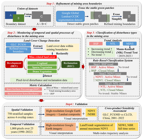
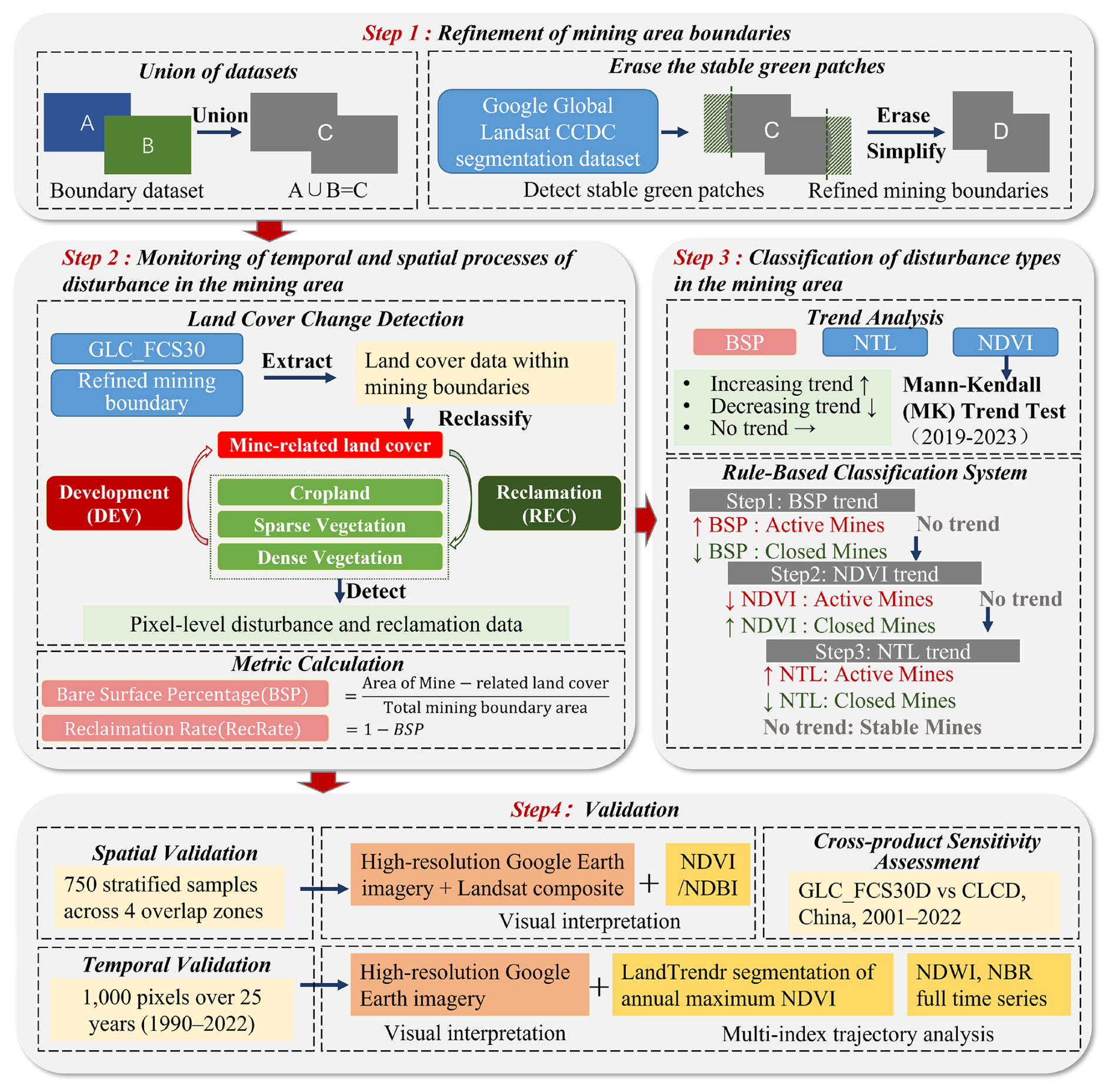
This study adopts an integrated strategy that combines multiple mining datasets with land change detection and morphological optimization to harmonize and refine surface mining boundaries, thereby deriving temporal indicators of mining activity. Temporal dynamics of land degradation and reclamation from 1985 to 2022 were further extracted, and a decision-tree algorithm was applied to determine the activity status of each mining patch. Figure 1 presents a detailed chart illustrating the workflow of this study. Four major steps can be distinguished: (1) Refinement of mining area boundaries; (2) Monitoring of temporal and spatial processes of disturbance in the mining area; (3) Classification of disturbance types in the mining area; (4) Validation.
2.1 Refinement of mining area boundaries
To enhance the accuracy of surface mining area boundaries, a multi-step preprocessing workflow was applied to refine the original global mining boundary dataset, encompassing data integration, classification reconstruction, stable green area exclusion, boundary overlap identification, and geometric simplification (Fig. 2).
2.1.1 Step 1
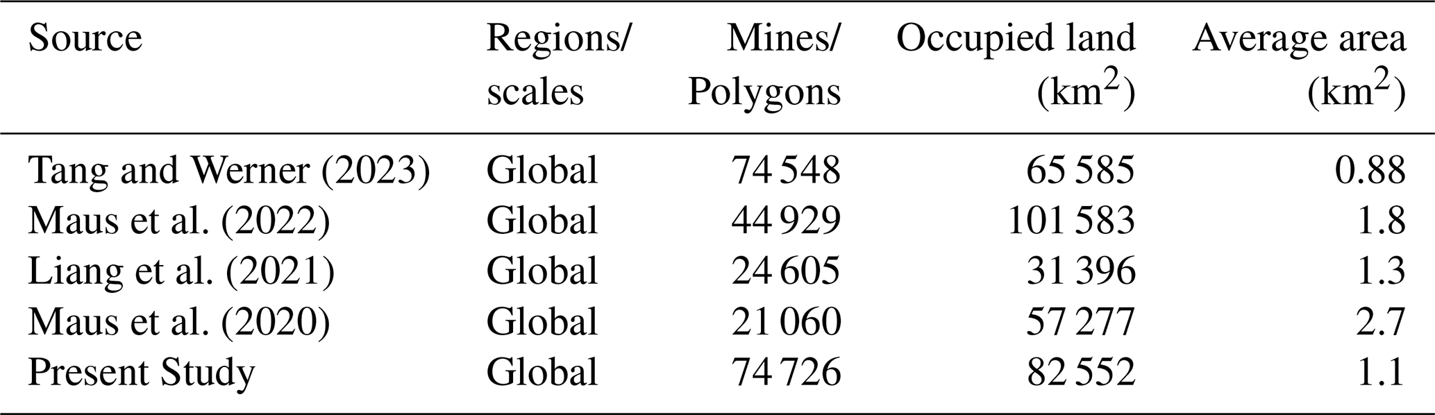
Dataset integration and removal of duplicate/intersecting areas. Two widely used global mining boundary datasets were first integrated: Dataset A (74 548 polygons, 65 585 km2) from Tang and Werner (2023) and Dataset B (44 929 polygons, 101 583 km2) from Maus et al. (2022). Through merging and union operations, a new Dataset C was generated, comprising 82 078 polygons covering 120 043 km2. This integration step relies on the spatial coverage of the two source mining inventories. The workflow is therefore designed to refine, harmonize, and remove overestimated portions of known mining areas, rather than to perform global discovery of mining sites absent from both input datasets. Mining areas that are missing from both sources cannot be recovered by the integration step and remain absent from the refined boundary product.
2.1.2 Step 2
Identification of stable green areas. To delineate truly disturbed regions within mining boundaries, we combined the Google Global Landsat-based CCDC Segments (1999–2019) (Gorelick et al., 2023) with a current-epoch land-cover map from the global 30 m land cover time-series dynamic remote sensing dataset (GLC_FCS30D) (Zhang et al., 2024) to extract areas with stable vegetation cover. This combination leverages long-term, consistent, and high-resolution observations to reliably extract areas of stable vegetation cover and detect mining-related vegetation changes. Pixels were labeled as stable green if they (i) exhibited no CCDC-detected temporal breakpoints across 1999–2019, and (ii) were classified as vegetated in the current land-cover map (e.g., forest, grassland, or cropland). This yields a mask of vegetated areas that remained unchanged over the past two decades. Spatially overlapping areas with mining boundaries were assumed to be undisturbed or ecologically restored and thus erased from the boundaries.
2.1.3 Step 3
Edge-area erasure strategy. Stable green pixels were aggregated into polygon objects, and erasure was performed at the object level. Only stable green polygons that intersected mining boundaries were erased to avoid misclassifying native or residual vegetation located along pit margins and haul-road edges as mining disturbance. Stable green polygons entirely enclosed within mining boundaries (i.e., not intersecting the boundary) were retained, as they likely represent enclosed features predating mining or non-mining inclusions rather than genuine reclamation or undisturbed zones. By erasing only boundary-intersecting polygons that showed no change during 1999–2019, we obtained the maximum potential mining disturbance boundary – the cumulative outer envelope of mining-induced land disturbance over the study period.
2.1.4 Step 4
Boundary jaggedness simplification and smoothing. Erasure of green polygons introduced jagged irregularities in boundary segments. A distance-thresholding method was applied for smoothing: adjacent boundary points within 100 m and approximately collinear were simplified into straight line segments, simplifying geometries. The final integrated mining boundary dataset contains 74 726 polygons with a total area of 82 552 km2.
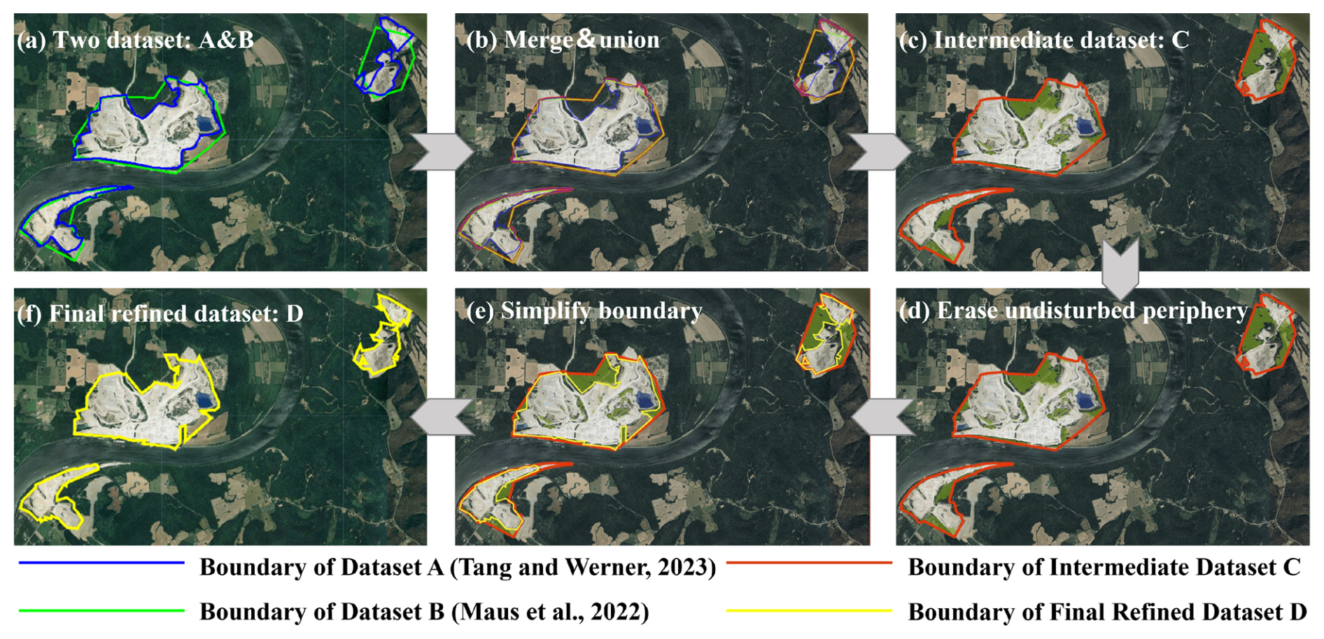
Figure 2Workflow of Refinement of mining area boundaries (Example Mining Area: 38.1353° N, 86.3544° W). (a) Two input datasets: Dataset A (blue lines; 74 548 polygons, 65 530 km2) (Tang and Werner, 2023) and Dataset B (green lines; 44 929 polygons, 101 583 km2) (Maus et al., 2022). (b) Merging and union of the two input datasets. (c) Intermediate Dataset C (red lines; 82 078 polygons, 120 043 km2); (d) Erasure of undisturbed peripheral areas. (e) Boundary simplification. (f) Final Refined Dataset D (yellow lines; 74 726 polygons, 82 552 km2). Imagery © 2025 Airbus, Landsat/Copernicus, Maxar Technologies; Map data © 2025 Google.
2.2 Monitoring the spatiotemporal dynamics of mining-induced disturbance
We analyzed land use changes within mining boundaries from 1985 to 2022 using the GLC_FCS30D dataset. For consistency with the objectives of this study, the original land cover classes were reclassified into four categories: (1) Mine-related land cover, (2) Cropland, (3) Sparse vegetation, and (4) Dense vegetation. Mine-related land cover was defined to include impervious surfaces, bare areas, consolidated bare areas, unconsolidated bare areas, water bodies and flooded flats, as identified in the GLC_FCS30D dataset.
We define DEV and REC based on the following land use type changes: if a pixel transitions from Cropland, Sparse vegetation, or Dense vegetation to Mine-related land cover, it is defined as a Development area. If a pixel transitions from Mine-related land cover to Cropland, Sparse vegetation, or Dense vegetation, it is defined as a Reclamation area. Using the land use definitions outlined above and the global 30 m land cover time-series dynamic remote sensing products (1985–2022), we obtained mining disturbance and reclamation data for over 74 726 surface mining polygons worldwide from 1985 to 2022, at 30 m pixel resolution. Rather than defining a site-specific baseline year for each mining polygon – which would be constrained by the general unavailability of comprehensive operational records for many global mining sites – we adopt a pixel-level detection approach. Disturbance is identified when a pixel first transitions from vegetated land cover to mine-related land cover within the study period (1985–2022). This first detected transition serves as the disturbance indicator, enabling fine-grained tracking of spatially and temporally heterogeneous mining impacts within individual polygons. GLC_FCS30D provides maps at five-year intervals before 2000 and annually thereafter. Pre-2000 transition timing was therefore interpolated, and annual area estimates before 2000 should be interpreted as interval-averaged estimates rather than directly observed annual changes. The resulting layers should therefore be interpreted as GLC_FCS30D-based land-cover transition products rather than as direct spectral–temporal breakpoint products. Because the workflow uses an existing global land-cover classification product as input, errors and uncertainties in the source LULC classes may propagate into the derived disturbance and reclamation layers. GLC_FCS30D was selected because, among currently available land-cover products, it uniquely combines global coverage, 30 m spatial resolution, annual temporal resolution after 2000, and an extended historical record back to 1985, which constitutes the combination of properties required for long-term, fine-resolution, global mining-dynamic analysis. We define Bare Surface Percentage (BSP) as the ratio of the area of Mine-related land cover to the total mining area boundary. Formally, it is expressed as:
This formulation assumes that a reduction in bare surface extent corresponds to vegetation regrowth or land cover restoration. It is important to note that this metric captures vegetation presence rather than comprehensive ecological reclamation. The reclamation rate (1− BSP) thus serves as a proxy for greening or revegetation progress within mining sites, and may overestimate the extent of true ecological restoration that includes soil quality recovery, biodiversity re-establishment, and ecosystem function restoration. It is important to clarify the terminology used in this study. We define three related but distinct concepts: (1) Greening refers to an increase in vegetation index values (e.g., NDVI) detected by remote sensing, indicating increased photosynthetic activity or vegetation cover, without implying ecosystem functionality; (2) Revegetation refers to the establishment of plant cover on previously disturbed land, whether through natural succession or active planting efforts; and (3) Reclamation in its comprehensive sense encompasses soil reconstruction, landform redesign, hydrological restoration, and the recovery of ecosystem structure and function. In this study, due to the limitations of remote sensing-based detection, what we identify as “reclaimed area” specifically refers to areas exhibiting vegetation recovery signals – essentially capturing greening or revegetation processes rather than comprehensive ecological reclamation.
2.3 Classification of mining areas based on development trends
To evaluate the recent developmental trajectories (2019–2023) and current status of global surface mining areas, we employed three indicators: NDVI, BSP, and NTL. NDVI was obtained from the MODIS MOD13Q1 and MYD13Q1 (Collection 6.1) products, and annual maximum NDVI composites at 250 m resolution were generated by combining Terra and Aqua observations for 2019–2023. The annual maximum value composite approach was adopted to minimize residual cloud contamination and to better represent peak vegetation conditions. BSP was calculated in this study based on the GLC_FCS30D dataset for 2019–2022. Nighttime light data were obtained from the VIIRS Day/Night Band monthly product (NOAA, dataset ID: NOAA/VIIRS/DNB/MONTHLY_V1/VCMSLCFG) via Google Earth Engine for 2019–2023. NDVI captures vegetation restoration or degradation, BSP quantifies bare land extent, and NTL reflects human activity intensity, enabling a comprehensive assessment of mining area disturbances and reclamation. All datasets were spatially harmonized and temporally aggregated to annual time series to ensure consistency across indicators. These indicators were then aggregated within each mining polygon to construct polygon-level annual time series for the Mann–Kendall trend analysis.
The Mann–Kendall (MK) trend test was employed to quantify the time-series trends of NDVI, BSP, and NTL in this study. This nonparametric statistical test is widely applied to detect monotonic trends in time-series data. The results of the analysis for each dataset are classified as follows: Increasing trend – indicating a significant positive trend (p< 0.1); Decreasing trend – indicating a significant negative trend (p< 0.1); No trend – indicating no statistically significant trend (p≥ 0.1). The results of the MK test are compiled into a unified DataFrame, with each mining area characterized by the trend classifications of NDVI, BSP, and NTL. Based on the combined trends of NDVI, BSP, and NTL, this study develops a rule-based decision-tree model to classify mining area disturbances.
-
BSP trend. As an indicator of bare land exposure, BSP is prioritized in the classification hierarchy. Mining areas with a decreasing BSP trend are classified as being in a reclamation state, while those with an increasing BSP trend are classified as being in an active mining state. Mining areas with no significant BSP trend are classified in the next step based on further analysis.
-
NDVI trend. NDVI is employed to assess vegetation restoration or degradation. Mining areas with an increasing NDVI trend are classified as being in a reclamation state, while those with a decreasing NDVI trend, reflecting vegetation loss, are classified as being in active mining. Mining areas with no significant NDVI trend are classified in the next step based on further analysis.
-
NTL trend. NTL is utilized to assess the level of human activities. Mining areas with an increasing NTL trend are classified as being in active mining, while those with a decreasing NTL trend indicate reduced human activities or mining area closure. If no significant NTL trend is detected, the area is classified as stable or undisturbed.
Based on trend analyses of NDVI, BSP, and NTL, a rule-based decision tree model was developed to classify mining areas into three categories. The framework first determined mining status as expanding, shrinking, or stable, and subsequently mapped these into types: active mines (expanding, characterized by increasing bare land, decreasing NDVI, and/or rising nighttime light signals), closed mines (shrinking, indicated by decreasing bare land, increasing NDVI, and/or declining nighttime light signals), and stable mines. The stable mines category encompasses: (1) equilibrium-state mines where extraction and reclamation have reached dynamic balance; (2) concurrent extraction-reclamation mines where simultaneous activities in different sectors produce offsetting signals; (3) maintenance-phase mines in transitional or suspended operational states; and (4) low-intensity or artisanal operations with insufficient signal magnitude to exceed statistical significance thresholds. By integrating the trend analyses of NDVI, BSP, and NTL, this study reveals the spatiotemporal dynamics of mining area disturbances and reclamations on a global scale.
2.4 Validation
The validation and sensitivity-assessment framework includes three ways to evaluate the performance and uncertainty of the proposed method: spatial validation, temporal validation, and cross-product sensitivity assessment. The spatial validation assessed the reliability of mining-area delineation by comparing our refined dataset with two existing global mining datasets through stratified cross-validation across four spatially defined zones. The temporal validation evaluated transition-year accuracy at sampled 30 m pixels using high-resolution Google Earth imagery, Landsat-based spectral trajectories with reference to the LandTrendr segmentation. The cross-product sensitivity assessment compared the GLC_FCS30D-based workflow with the same conceptual transition rules applied to CLCD over Chinese mining polygons, thereby quantifying uncertainty attributable to the choice of source LULC product.
To quantitatively assess the accuracy improvements of the refined dataset compared to the source datasets, we designed a stratified cross-validation framework based on the spatial overlap relationships among the three datasets: Dataset A (Tang and Werner, 2023), Dataset B (Maus et al., 2022), and our refined Dataset D. Four validation zones were defined based on dataset agreement patterns (Fig. 3):
-
Zone A. Areas identified by both Tang and Maus but excluded in our refined dataset, representing potentially over-estimated mining extents in the source datasets;
-
Zone B. Three-way consensus areas identified by all three datasets;
-
Zone C. Areas identified by Maus and our dataset but not by Tang;
-
Zone D. Areas identified by Tang and our dataset but not by Maus.
A total of 750 validation points (Fig. A1) were randomly sampled across these zones using stratified random sampling (150 points each for Zones A, C, and D; 300 points for Zone B to ensure adequate representation of consensus areas). Each point was verified through visual interpretation of high-resolution Google Earth imagery, supplemented by Landsat 8/9 Collection 2 Level 2 surface reflectance imagery (July 2019 to June 2021). Cloud-free median composites were generated using true-color visualization (bands B4, B3, B2), and the Normalized Difference Vegetation Index (NDVI) and Normalized Difference Built-up Index (NDBI) were calculated to assist in distinguishing mining areas from vegetated or built-up land covers.
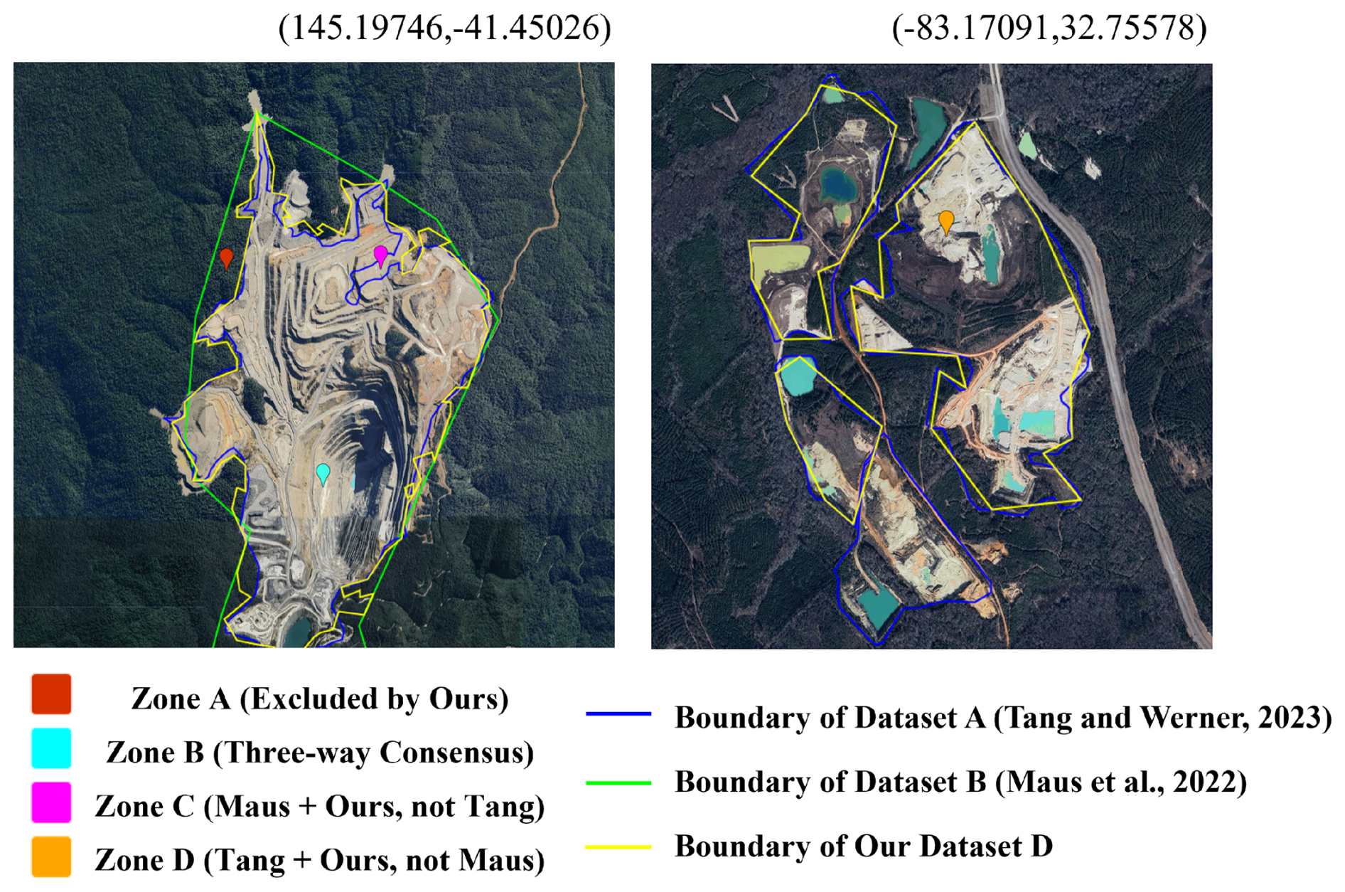
Figure 3Illustration of the four validation zones defined by spatial overlap relationships among three mining datasets at two representative sites. Left: a mining site in Tasmania, Australia (145.197° E, 41.450° S); Right: a mining site in Georgia, USA (83.171° W, 32.756° N). The boundary lines represent mining area delineations from Dataset A (Tang and Werner, 2023; blue), Dataset B (Maus et al., 2022; green), and our refined Dataset D (yellow). The filled zones indicate: Zone A (red) – areas identified by both source datasets but excluded in our refined dataset; Zone B (cyan) – three-way consensus areas identified by all three datasets; Zone C (magenta) – areas identified by Dataset B and our dataset but not by Dataset A; Zone D (orange) – areas identified by Dataset A and our dataset but not by Dataset B. Imagery © 2026 Airbus, CNES/Airbus, Landsat/Copernicus, Maxar Technologies; Map data © 2026 Google.
To assess the accuracy of the detected transition years, we constructed a reference set of 1000 samples drawn from mining-related pixels at which the dataset reports a development or reclamation transition. To maintain temporal balance across the study window, 40 pixels were randomly selected for each of 25 nominal transition years or time steps (1990, 1995, and 2000–2022), giving a total of 1000 validation samples whose spatial distribution is shown in Fig. A2. Reference transition years were assigned through visual interpretation of the available high-resolution Google Earth imagery time series, supported by Landsat-based spectral trajectories. Specifically, we used Landsat Collection 2 Level-2 surface reflectance data from Landsat 4, 5, 7, 8, and 9 for the period 1985–2024. Surface reflectance values were scaled using the Collection 2 scale factors, and clouds, cloud shadows, and saturated pixels were masked using the QA_PIXEL and QA_RADSAT bands. For each valid Landsat observation, we calculated NDVI together with complementary Normalized Difference Water Index (NDWI) and Normalized Burn Ratio (NBR) to assist the interpretation of disturbance and recovery signals. Annual maximum NDVI composites were further generated and segmented using the LandTrendr algorithm to identify major breakpoints in the vegetation trajectory. The final reference transition year for each validation sample was determined by jointly considering the high-resolution imagery record, the LandTrendr segmentation result, and the multi-year Landsat spectral-index profiles. The accuracy metric reported in Figure A7 is the offset between the dataset's predicted transition year and the trajectory-derived reference transition year, evaluated under explicit temporal tolerance windows.
The spatial location of the sample and the accuracy verification results using NDVI, NBR, NDWI, and high-resolution Google Earth imagery are presented in Fig. 4. Figure 4a illustrates the location of the sample mine on the island of Borneo in Indonesia. The spectral trajectories indicate a stable condition before 2015, followed by clear disturbance signals in 2015. The mining year inferred from the LCTS, however, is 2018, highlighting the potential temporal discrepancy between spectral evidence and land cover-based detection.
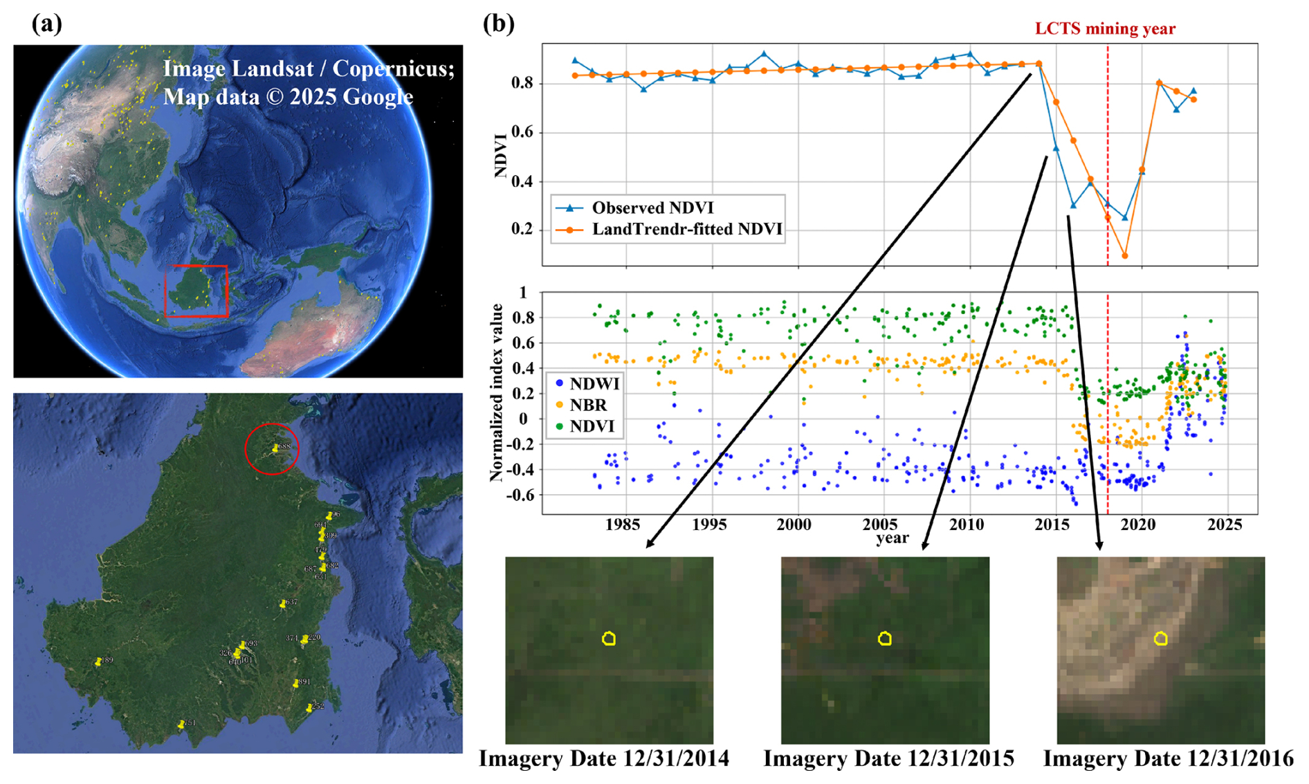
Figure 4(a) Spatial location of a sample mine (WGS84: 3.552883° N, 117.169372° E) located on the island of Borneo, Indonesia. (b) Spectral validation results for the selected sample point (Point 688). The upper panel displays the NDVI time series (blue), LandTrendr segmentation results (orange), and the mining year inferred from the land cover time series (LCTS) indicated by a red vertical dashed line. The lower panel shows high-resolution Landsat 8 OLI imagery (Collection 2 Level-2 Surface Reflectance) downloaded directly from Google Earth Engine for 2014, 2015, and 2016. The yellow marker indicates the location of the 30 m validation pixel. Imagery was exported at 10 m resolution (3 × supersampling) to enhance visual clarity while maintaining spectral fidelity of the original 30 m Landsat data.
In addition, to assess how strongly the inferred mining transitions depend on the choice of source land-cover product, we performed an object-based cross-product sensitivity assessment using the China Land Cover Dataset (Yang and Huang, 2021). CLCD provides 30 m annual maps over 1985–2025 for China, classified independently of GLC_FCS30D using a 9-class scheme and distinct temporal-consistency rules. The comparison was restricted to the 27 948 Chinese mining polygons of our dataset over 2001–2022, the temporal window in which both products provide annual maps; the pre-2000 period was excluded because GLC_FCS30D is delivered as five-year snapshots there (1985, 1990, 1995), and a comparison with CLCD's annual maps in that period would primarily reflect this temporal-resolution mismatch rather than classifier-driven differences. We applied the same conceptual transition rule used for the GLC_FCS30D-based DEV/REC layers, with class equivalence mapped to CLCD's class system. In CLCD, the mine-related class group comprised classes 5 (Water), 7 (Barren) and 8 (Impervious), and the vegetation/cropland class group comprised classes 1 (Cropland), 2 (Forest), 3 (Shrub), 4 (Grass) and 9 (Wetland). For each mining polygon we recorded, separately for development and reclamation, the total transition area in each product, the area-weighted mean transition year in each product, the polygon-level co-detection status, the area ratio CLCD/GLC_FCS30D, and the absolute polygon-mean transition-year offset between products in co-detected polygons.
3.1 Spatial distribution characteristics of global mine areas
Global surface mining exhibits pronounced spatial heterogeneity in both scale and intensity. At the continental and national levels, mining activities are unevenly distributed, with certain regions concentrating a disproportionately large number of sites or total area. Distinct spatial patterns also emerge, reflecting divergent development models – ranging from fragmented small-scale operations in Asia to centralized large-scale mines in countries such as Australia and Brazil. Beyond these spatial trends, a critical ecological concern arises from the overlap between mining areas and Key Biodiversity Areas (KBAs), where intensive extraction activities directly threaten globally significant ecosystems and species (Boldy et al., 2021; Li et al., 2020; Lv et al., 2019; Sonter et al., 2018; Tai et al., 2020).
This study identifies 74 726 surface mine area polygons globally, encompassing a cumulative areal extent of 82 552 km2, with an arithmetic mean of 1.10 km2. Figure 5a illustrates the global distribution of mining polygons, together with their area and count aggregated along latitude and longitude. Figure. A3 shows the global mining density in a 100 km grid. The analysis was performed in an equal-area projection (Interrupted Goode Homolosine), while the visualization uses the PlateCarree projection. Mining area densities range from 0 % to 15.13 % per fishnet, at an average of 0.19 %.
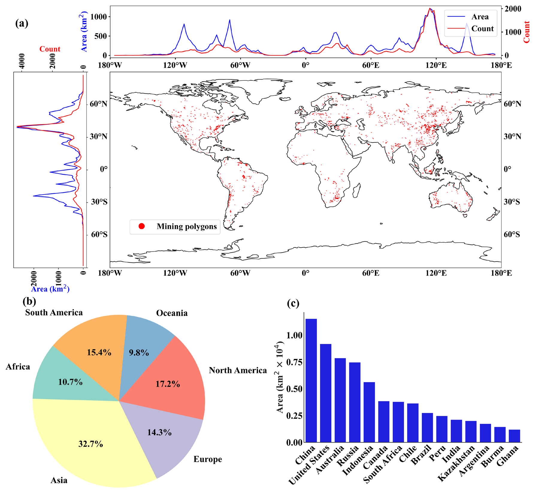
Figure 5Global distribution and characteristics of mining polygons. (a) Global distribution of mining polygons and their latitudinal/longitudinal statistics of area and count. Given the visualization effect, the centroids of the polygons are used for display here instead of the actual shapes of the polygons. (b) Continental proportion of the global mining polygons area. (c) Mining polygons area in the top 10 countries in terms of total mining area.
Asia hosts the largest share in both number and areal extent, with 37 304 polygons (49.9 %) spanning 26 992 km2 (32.7 %), and an average site size of 0.72 km2, indicating highly fragmented, small-scale mining (Fig. 5b). North America ranks second, comprising 11 059 polygons (14.8 %) and 14 160 km2 (17.2 %), with a mean site size of 1.28 km2. Europe accounts for 9167 polygons (12.3 %) over 11 799 km2 (14.3 %), with a mean site size of 1.29 km2. Africa (6360 polygons, 8.5 %; 8801 km2, 10.7 %) and South America (6923 polygons, 9.3 %; 12 345 km2, 15.4 %) exhibit comparatively larger average site sizes (1.38–1.78 km2) due to widespread surface mining. In Oceania, dominated by Australia's mega-mines, 3913 polygons (5.2 %) extend over 8075 km2 (9.8 %), with the largest mean site size globally (2.06 km2).
The distribution of global mine areas is markedly uneven, with a strong concentration in a limited number of countries. Our dataset comprises mine area polygons from 155 countries and regions. Table A1 shows summary of per-country mine areas globally mapped in this study. The top 10 countries ranking by total mining area, including China, the United States, Australia, Russia, Indonesia, Canada, South Africa, Chile, Brazil, and Peru, comprise 70.6 % (58 268 km2) of the global total. When extended to the top 30 countries, this proportion increases to 90.7 % (74 915 km2), underscoring the high geographical concentration of mining activities worldwide. Table A1 presents the mining areas of the major contributing countries. China ranks first in total mining area (11 542 km2, 14 %), driven by 27 948 mining polygons with a mean areal extent of 0.41 km2 per site (Fig. 5c). While China has the largest number and total area of mining polygons globally, its average site size remains significantly lower than that other high mineral demand countries (e.g., India and USA) and high mineral export countries (e.g., Australia, Canada, South Africa, and Russia), where averages exceed 1 km2. African countries, particularly in sub-Saharan Africa, show both small total areas and small scale sizes, largely due to the prevalence of artisanal and small-scale mining that occurs informally on unregulated land (Hilson et al., 2017; Oramah et al., 2015).
In this study, a total of 3248 mining areas were identified within KBAs worldwide, covering a combined area of 3986 km2, accounting for 4.8 % of the global mining extent. Figure 6a shows the global mining density within KBAs in a 100 km grid. These polygons are unevenly distributed across 105 countries and regions. Mining area densities range from 0 % to 3.25 % per fishnet, at an average of 0.07 %. Table A2 shows summary of per-country mine areas within KBAs mapped in this study. Asia hosts the largest number of KBA-overlapping mining areas (1412 polygons, 43.5 %), followed by South America (543 polygons), North America (394 polygons), and Europe (390 polygons). In terms of area, Asia also ranks highest (1299 km2, 32.7 %), followed by South America (1156 km2, 28.9 %) and Africa (512 km2, 12.9 %) (Fig. 6b). Approximately 71 % of the polygons are situated within 10 countries: China, Brazil, Argentina, Mexico, Australia, South Africa, Indonesia, Namibia, Burma, and Venezuela (Fig. 6c). China alone accounts for 858 mining areas (26.3 %) within KBAs, with a total area of 682 km2 (17.1 %). Brazil (244 polygons, 443 km2) and Argentina (22 polygons, 427 km2) also show considerable overlaps area despite fewer polygons. Notably, Argentina shows largest average area per polygon (19 km2), indicating the presence of large-scale operations within sensitive ecological regions. In contrast, countries such as Australia and Mexico exhibit moderate overlap both in terms of site count and area. These results highlight spatial clustering of mining pressure within biodiversity-priority regions, particularly in Asia and South America. The coexistence of high biodiversity value and intensive mining underscores the urgent need for spatially targeted conservation strategies and the integration of ecological sensitivity into mining governance frameworks.
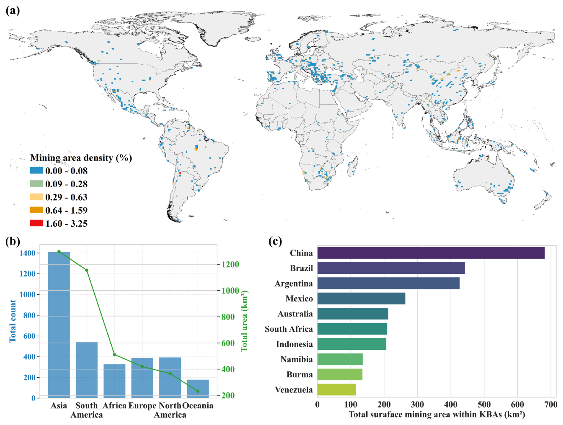
Figure 6Global distribution and characteristics of mining polygons within KBAs. (a) Global mining density within KBAs in a 100 km grid. Mining area density is calculated as the proportion of mining area within 100 × 100 km (10 000 km2) grid cells. Data was aggregated using the Interrupted Goode Homolosine equal-area projection to ensure accurate area calculations. The map is displayed using the PlateCarree projection. The boundary and attribute data of KBAs used in this study are obtained from the World Database of Key Biodiversity Areas (https://www.keybiodiversityareas.org/, last access: 18 August 2025). (b) Counts and total area of mine within KBAs by world regions. (c) Top 10 countries by mining area within KBAs.
3.2 Monitoring of spatiotemporal process of disturbance in mining area
Mining activities lead to substantial modifications in land cover. By tracking land cover change at the pixel level within delineated mining boundaries, we analyzed the global spatiotemporal dynamics of land disturbance and reclamation from 1985 to 2022. Over this period, the cumulative area of land disturbed by surface mining reached 40 596 km2, accounting for approximately 49 % of the total global surface mining footprint. In comparison, the reclaimed area totalled 29 285 km2. The annual land disturbance and reclamation areas showed distinct temporal dynamics during 1985–2022, with phase shifts in both magnitude and relative balance (Fig. 7a).
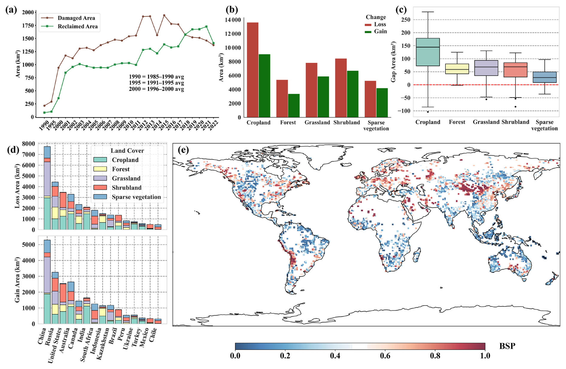
Figure 7(a) Annual land disturbance and reclamation area of global surface mines (1985–2022). To ensure the continuity of the graph, the values for 1990, 1995, and 2000 correspond to the average annual changes over five-year intervals – specifically, they represent the five-year averages for the periods 1985–1990, 1991–1995, and 1996–2000, respectively. (b) Gain and loss of land cover types during mining disturbance events. (c) Boxplot of “gap” for land cover types (gap = loss − gain). (d) Losses and gains of five land cover types in the top 15 countries ranked by total area of land with changes. (e) Percentage of bare surface area in global mining areas, aggregated to 100 km resolution (2022).
From 1985 to 2000, for the mine areas included in the study, the annual disturbed area surged from 214 to 940 km2, while the annual reclamation area expanded more slowly from 82 to 357 km2, resulting in a substantial gap indicative of delayed ecological restoration. During 2001–2010, both metrics continued rising to 1541 km2 (disturbance) and 1030 km2 (reclamation) with decelerated rates (36.7 km2 vs. 18.4 km2 yr−1), and the positive gap narrowed gradually. From 2011 onward, the disturbed area exhibited pronounced fluctuations, peaking at 1943 km2 in 2015, followed by a steady decline to 1373 km2 in 2022. In contrast, the reclaimed area continued to rise with interannual variability and reached a maximum of 1735 km2 in 2021. A notable transition occurred in 2018, when the reclaimed area (1576 km2) first exceeded the annual disturbed area (1569 km2), marking a shift toward net ecological recovery. This turning point underscores a global shift toward intensified ecological restoration. For example, in China, ecological rehabilitation of mining areas has long been prioritized, with national programs over the past four decades focusing on vegetation recovery and the mitigation of geological hazards. Furthermore, the Chinese government has ordered the closure of over 20 000 mines, and these sustained efforts have led to significant advances in mine land reclamation (Chen et al., 2025a; Xiao et al., 2020c). Quantification of the disturbance-reclamation gap (i.e., disturbance area minus reclamation area) confirms consistent positive values (net degradation) during 1990–2017, shifting to negative values post-2018, indicating a global transition to net land recovery.
We analyzed land disturbance and reclamation in global surface mining areas across five landcover types: cropland, forest, grassland, shrubland, and sparse vegetation from 1985 to 2022. Cropland had the largest damaged area (13 623 km2, 33.6 %), followed by shrubland (8464 km2, 20.9 %), grassland (7836 km2, 19.3 %), sparse vegetation (5262 km2, 13.0 %), and forest (5411 km2, 13.3 %) (Fig. 7b). For land reclamation, cropland also boasted the largest cumulative reclaimed area (9082 km2, 31.0 %), with shrubland (6716 km2, 22.9 %), grassland (5885 km2, 20.1 %), sparse vegetation (4221 km2, 14.4 %), and forest (3380 km2, 11.5 %) following in sequence. Despite ongoing reclamation efforts, considerable differences remain between disturbed and restored land cover types. Here, “reclamation” refers to areas showing vegetation recovery signals detected via land cover transitions, which may result from active restoration practices, natural regrowth (revegetation) in abandoned polygons, or conversion to agricultural land. This metric captures greening trends rather than verified comprehensive ecological restoration. We calculated the gap between damaged and reclaimed areas for annual areas of each landcover type (Figs. A4 and 7c). As of 2022, approximately 4541 km2 of cropland (33.3 %) and 2039 km2 of forest (37.5 %) were disturbed by unreclaimed mining areas. In contrast, the unreclaimed proportions for grassland, shrubland, and sparse vegetation are relatively lower, at 24.9 %, 20.7 %, and 19.8 %, respectively. This discrepancy may reflect differences in post-mining land use suitability, ecological fragility, or restoration policies targeting specific land cover types.
Notably, although the forest had the lowest damaged area among all land types, the gap between its disturbance and reclamation showed a relatively compact and continuously positive distribution. The box plot revealed that the net gap in most years was concentrated in the 0–100 km2 range, with almost no extreme outliers, reflecting the overall low disturbance intensity of forest ecosystems. However, unlike other landcover types where reclaimed area exceeded damaged area in some years, the forest was almost in a “net damage” state throughout the year. This persistent reclamation lag may stem from the long natural recovery period of forests or insufficient current restoration measures for forest ecosystems (Poorter et al., 2021). Moreover, considering the crucial role of forests in biodiversity protection and carbon storage, even a small absolute damaged area can have significant ecological consequences per unit of disturbance (Cook-Patton et al., 2020; Feng et al., 2022).
Among all mining-induced land disturbances globally, Asia contributed the largest share, particularly in cropland and grassland areas. Approximately 6414 km2 of disturbed cropland (47.1 % of the global total) and 4532 km2 of disturbed grassland (57.8 %) were located in Asia (Fig. A5). Within the region, China ranked first in both disturbed and reclaimed land areas, accounting for about 21.7 % of global cropland loss and 40.5 % of global grassland loss (Fig. 7d). Besides, forest disturbances were primarily observed in Russia, Canada, and Indonesia, contributing 19.8 %, 12.7 %, and 11.4 % of the global total, respectively. Shrubland loss was concentrated in North America (24.9 %) and Africa (23.4 %), with the United States alone contributing 16.5 %.
By 2022, the global average reclamation rate of surface mining land reached 62.6 %. In this study, the reclamation rate was calculated as 1− BSP, where BSP represents the proportion of mine-related bare surface classes within each mining polygon. National and global values were calculated as area-weighted averages using the mining polygon area. Therefore, this metric should be interpreted as a land-cover-based indicator of reclamation status rather than a direct field measurement of ecological restoration. The spatial pattern shown in Fig. 7e indicates that unreclaimed or actively disturbed mining surfaces remain concentrated in several major mining regions, including northern China, Central Asia, eastern Europe, western North America, the Andes, southern Africa, and parts of Australia. In contrast, many mining regions in Southeast Asia, tropical South America, parts of Africa, and Oceania showed lower proportions of exposed mine-related bare surfaces, suggesting a higher degree of land-cover recovery within mapped mining polygons.
At the national level, the top 15 countries ranked by mapped surface mining area showed substantial differences in reclamation rates (Fig. A6). Among these countries, Ghana (93.7 %) and Indonesia (92.1 %) showed the highest reclamation rates, followed by Australia (80.8 %), Brazil (78.8 %), South Africa (73.1 %), India (69.1 %), Peru (68.9 %), and the United States (65.9 %), all exceeding the global average. In contrast, China (46.6 %), Chile (17.3 %), Canada (55.3 %), Kazakhstan (56.6 %), and Russia (57.5 %) were below the global average, indicating that large surface mining footprints do not necessarily correspond to high reclamation rates. China, which contains the largest number of mapped mining polygons globally, had a reclamation rate substantially below the global average, highlighting the continuing restoration pressure associated with high-intensity mining. Chile showed the lowest reclamation rate among the top 15 countries, consistent with the concentration of large exposed mining surfaces in the Andes.
3.3 Classification of global surface mining areas
Overall, the global distribution of mining development status reveals a dominant trend of active mining, both in terms of site counts and spatial extent, with notable regional and national variations. Figure 8a presents the classification of the development status of mining areas over the recent years, encompassing three categories: active, stable, and closed.
Globally, of the 74 726 surface mining polygons identified, 14 546 (19.5 %) were classified as closed mines, 36 542 (48.9 %) as stable mines, and 23 638 (31.6 %) as active mines (Fig. 8b). The proportion of stable mines (48.9 %) is notably lower than that reported in comparable global analyses; for example, Wang et al., (2025), using single-indicator NDVI-based classification, identified 64.3 % of mines as stable. This 15-percentage-point reduction demonstrates the enhanced sensitivity of our multi-indicator approach in detecting mining dynamics that would otherwise remain undetected. In terms of area, active mines accounted for 30 147 km2 (36.5 % of the global total), followed by closed mines at 25 389 km2 (30.8 %). These results indicate that active mining areas dominate both numerically and in spatial extent worldwide. Regional analysis (Fig. 8c) shows that active mines outnumber closed mines across all continents except Europe, which is the only continent having more closed mines (2003) than active mines (1885). Mineral-rich Africa exhibits the lowest proportion of closed mines (18.7 %) and the highest proportion of active mines (33.5 %) (Ross and Werker, 2024). Asia has approximately 20.0 % of green mines and 32.0 % active mines, with 11 953 active mines representing 50.6 % of the global active mine count, highlighting intensive mining operations. In North America, active mines constitute 33.5 % of polygons, underscoring their role as major mineral producers (Giljum et al., 2025).
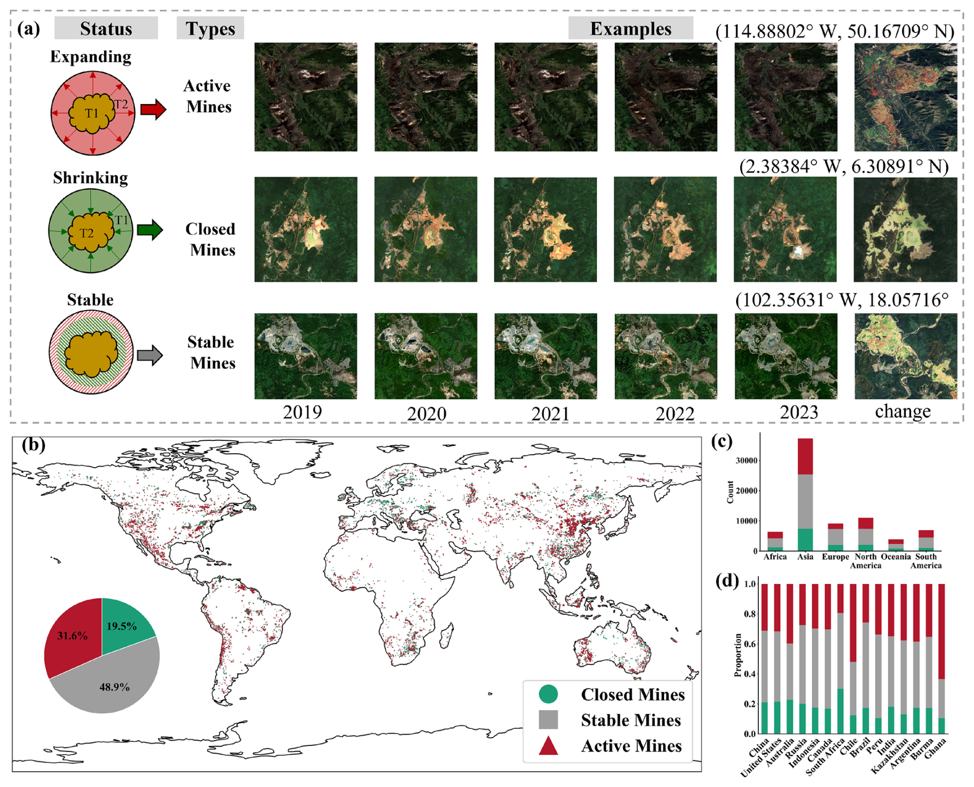
Figure 8(a) Classification of development status of mining areas in the recent five years: active, stable, closed. For the change maps corresponding to each development status category, two distinct change directions are denoted by specific colors: Red pixels indicate a land cover transition from non-mining-related types to mining-related types, representing the expansion of mining areas. Green pixels indicate the inverse transition – from mining-related land cover types to non-mining-related types – representing the shrinkage of mining areas. (b) Global distribution of three types of mining areas. Each mining area is represented by its centroid marker. Closed, stable, and active mining areas are shown using different colors and marker shapes. (c) Continental counts of mining areas types (d) Type structures of the top 15 countries, sorted by the total number of mining areas in descending order. In panel (a), the annual true-color images and the corresponding change maps were produced by the authors and contain modified Copernicus Sentinel data 2019–2023.
Among the major mining countries, almost all exhibit a predominance of active mines over closed mines, indicating that most nations remain in an expansionary phase of mining development (Fig. 8d). Fourteen of the fifteen leading mining countries follow this pattern, with South Africa as the sole exception. Several major mining nations, including China, the United States, Australia, Russia, Indonesia, and Canada, show a markedly higher proportion of active mines relative to closed mines. China, which possesses the largest mining area globally, and the United States, ranking second, both display similar proportions, with active mines accounting for approximately 31 % and closed mines around 21 %. Chile has the highest share of active mines (52.0 %) and one of the lowest shares of closed mines (12.4 %), reflecting its copper-dominated sector's strong reliance on ongoing mineral extraction (Abbas et al., 2024). Peru shows a similar trend, with closed mines comprising only 10.4 % and active mines 33.8 %. In contrast, South Africa stands out as the only major mining country where closed mines (30.1 %) exceed active mines (19.4 %), diverging from the overall global trend.
4.1 Comparison of results of prior mining area datasets
Our refined global surface mining area dataset demonstrates substantial improvements in comprehensiveness, offering detailed insights into spatiotemporal processes related to mining and reclamation. Compared with existing datasets, it achieves greater completeness in terms of data volume, while also filling the gap in long-term spatiotemporal change information of mining - induced land disturbances?.
To evaluate its performance, we systematically compared our dataset against two widely used global mining boundary datasets – Dataset A (Tang and Werner, 2023) and Dataset B (Maus et al., 2022) – as well as the intermediate merged dataset (Dataset C) generated during our workflow (Fig. 2). Dataset A comprises 74 548 polygons (65 585 km2) and delineates mining areas with relatively tight outlines, thereby capturing polygon shape variability in detail. In contrast, Dataset B consisting of 44 929 polygons (101 583 km2), applies a 10 km manual buffering approach that broadly encompasses mining extents but frequently exaggerates disturbed areas. These methodological differences are evident in Fig. 2a, where the boundaries from Maus et al. (2022) (green lines in Fig. 2a) cover much larger regions, whereas the boundaries from Tang and Werner (2023) (blue lines in Fig. 2a) are more closely aligned with actual mine features. Building on these, the boundaries of our refined dataset (yellow lines in Fig. 2f) further improve delineation by more accurately fitting the true extent of mining disturbances, thereby reducing both overestimation and omission.
Our intermediate Dataset C, obtained through merging and union operations, contained 82 078 polygons (120 043 km2), which maximized spatial coverage but introduced redundancy and misclassification. Through multi-step optimization, we refined this dataset to 74 726 polygons (82 552 km2), thereby striking a balance between coverage and accuracy. Compared with Maus et al. (2022), our dataset contains 165 % of its polygons while covering only 81.3 % of its total area, effectively reducing boundary overestimation. Relative to Tang and Werner (2023), our dataset adds 178 polygons and represents 125.9 % of its mapped area. By integrating CCDC-derived land surface dynamics with fine-resolution land cover datasets, we erased long-term stable vegetation patches and eliminated spurious inclusions, which led to a 31.2 % reduction (37 493 km2) in overestimated areas compared with the simple merged result. This refinement yields the maximum potential mining disturbance boundary, defined as the cumulative outer envelope of mining-induced land disturbance across the study period, thereby substantially improving boundary precision. As summarized in Table 1, the refined dataset (present study) balances spatial coverage and accuracy, reducing both overestimation and omission, and thus provides a more reliable basis for global-scale mining disturbance assessments.
Recently, Sepin et al. (2025) introduced a machine learning-based dataset mapping mining areas in the tropical belt from 2016 to 2024. Their approach employs a SegFormer model trained on the Tang and Werner (2023) and Maus et al. (2022) datasets to automatically segment mining areas from high-resolution (< 5 m) Planet/NICFI satellite imagery. The resulting dataset comprises approximately 147 000 mining polygons covering an average annual area of 66 400 km2 within the tropical belt.
For comparative analysis, we extracted mining polygons from our dataset within the same tropical region (±30° latitude), yielding 25 772 polygons covering 37 744 km2. In comparison, the Sepin et al. (2025) dataset contains 16 842 polygons with an area of 66 835 km2 for the year 2020. The substantially larger average polygon size in Sepin et al. (2025) reflects their discovery-oriented approach, which prioritizes detection sensitivity over boundary precision. Their machine learning predictions can identify previously unmapped sites, including informal and artisanal mining operations, but inevitably include model uncertainty and potential commission errors.
In contrast, our approach is designed for tracking – monitoring land cover dynamics within known mining footprints through morphological optimization and systematic removal of stable vegetation. Visual comparison at representative mining sites (Fig. 9) reveals that the Sepin et al. (2025) predictions exhibit notable omission errors at large-scale industrial mines, with fragmented boundaries that miss substantial portions of active mining areas visible in Landsat imagery. This observation aligns with their training strategy, which relied on existing polygon datasets that may underrepresent certain mining configurations.
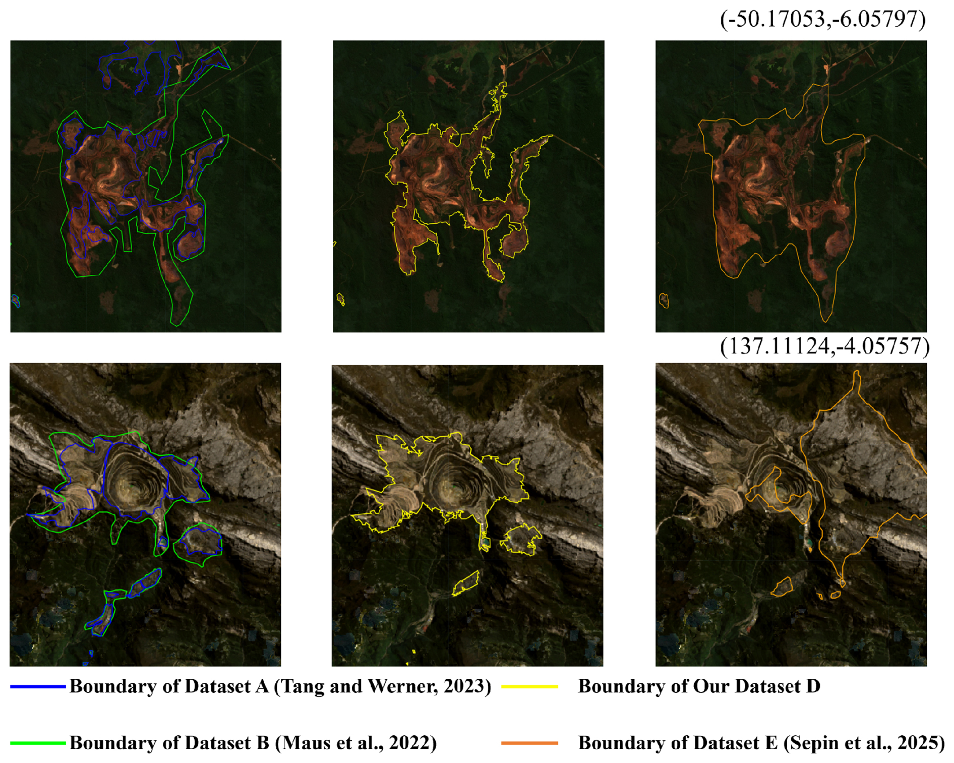
Figure 9Comparison of mining area boundary delineations among four datasets at two representative tropical mining sites. Top row: Carajás Iron Mine, Brazil (50.171° W, 6.058° S); Bottom row: Grasberg Mine, Indonesia (137.111° E, 4.058° S). Each row displays three panels showing different dataset combinations: left panel – Dataset A (Tang and Werner, 2023; blue) and Dataset B (Maus et al., 2022; green); middle panel – our refined Dataset D (yellow); right panel – Dataset E (Sepin et al., 2025; orange). Background imagery: Landsat 8 OLI true-color composite (2020). The comparison illustrates that our refined boundaries (yellow) achieve tighter alignment with visible mining features, while the Sepin et al. (2025) predictions (orange) exhibit omission errors at both sites, missing substantial portions of active mining areas.
The two datasets thus serve complementary purposes. Sepin et al. (2025) provides valuable coverage of artisanal mining and near-real-time detection capability in the recent period (2016–2024), while our dataset offers greater boundary precision, broader geographic scope (global vs. tropical), and substantially longer temporal depth (1985–2022). For ecological impact assessment and reclamation monitoring – the primary objectives of our study – the conservative boundary delineation minimizes false positives and provides robust baselines, even if this approach may underestimate total mining extent in regions with prevalent informal mining activity.
In this study, we analyzed the spatiotemporal dynamics of 74 726 mining polygons worldwide, covering the period from 1985 to 2022, and further examined recent development trends of mining areas. The monitoring of mining disturbance and reclamation processes was conducted at the pixel scale, enabling fine-grained tracking of temporal land-use transitions within each mining site. By comparison, Yu et al. (2018) focused on the spatial locations of 790 mines and carried out time-series monitoring of land-cover changes, but its temporal coverage was limited to the 1980s–2013. Our dataset not only extends the temporal span to nearly four decades (1985–2022) but also substantially broadens the scope to a global coverage of 74 726 mining polygons. In addition, we classified the current development status of mines into three categories – active, closed, and stable – providing a new dimension of information that complements previous datasets. The broader spatial coverage, combined with improved temporal resolution and accuracy, offers enhanced capacity to track fluctuations in both mining expansion and reclamation. This advancement facilitates a more comprehensive understanding of the temporal evolution of global surface mining disturbances and establishes a stronger foundation for ecological restoration research and impact assessment in mining regions.
The cross-dataset validation results provide quantitative evidence for the accuracy improvements achieved by our boundary refinement approach (Table 2). Zone A, representing areas identified by both Tang and Maus but excluded in our refined dataset, exhibited a mining rate of only 28.7 % (43 out of 150 samples). This indicates that 71.3 % of the areas excluded by our refinement process were correctly identified as non-mining land covers, validating the effectiveness of our CCDC-based stable vegetation exclusion strategy in reducing commission errors inherited from the merged dataset. Zone B, the three-way consensus area, showed a mining rate of 91.3 % (274 out of 300 samples), confirming the high reliability of areas where all three datasets agree. This high accuracy in consensus areas provides a solid foundation for the subsequent time-series analysis of mining disturbance and reclamation dynamics. Zones C and D demonstrated mining rates of 81.3 % (122/150) and 86.0 % (129/150), respectively. These results suggest that our integrated dataset successfully captures additional mining areas that were missed by individual source datasets while maintaining reasonable accuracy. The slightly higher mining rate in Zone D compared to Zone C may reflect differences in the mapping strategies employed by Tang and Werner (2023) and Maus et al. (2022).
Table 2Cross-dataset validation results for boundary refinement assessment.
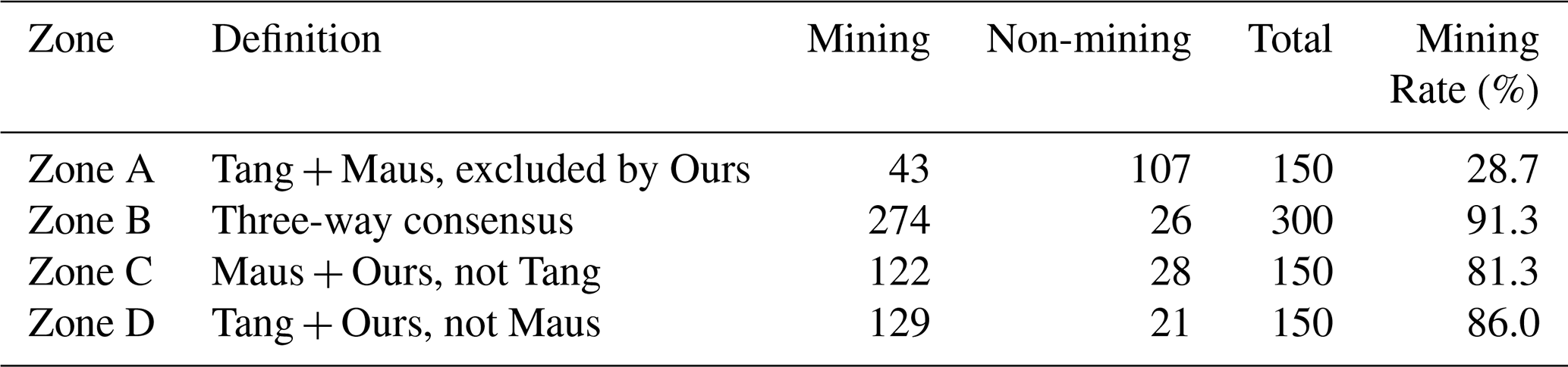
Collectively, these validation results demonstrate that our boundary refinement approach achieves two key objectives: (1) effectively reducing commission errors (false positives) from the merged dataset, as evidenced by the substantial proportion of non-mining areas in Zone A (71.3 %); and (2) preserving genuine mining areas with high confidence, as indicated by the consistently high mining rates in Zones B, C, and D (81.3 %–91.3 %). This balance between precision and coverage represents a meaningful improvement over using either source dataset alone or a simple union of both.
4.2 Advantages of this method and future application directions
By integrating and refining existing datasets and applying automated morphological optimization, this study substantially improved both the coverage and boundary accuracy of global surface mining area delineation relative to previous products. Specifically, the delineated boundaries were enhanced by erasing stable green pixels – identified through the Google Global Landsat-based CCDC Segments (1999–2019) and the GLC_FCS30D dataset – that intersected with mining polygons over a 20-year period. This procedure effectively reduced misclassification of non-mining vegetation within mining extents, thereby increasing the spatial precision of boundary mapping. As a result, we derived the maximum potential mining disturbance boundary, defined as the cumulative outer envelope of mining-induced land disturbance throughout the study period. This approach not only ensures more reliable detection of historical mining footprints but also provides a solid data foundation for future monitoring of disturbance–reclamation dynamics at multiple spatial and temporal scales.
For classifying development trends of mining areas, we integrated three remote sensing-derived indices, NDVI, BSP, and NTL, that capture spatiotemporal changes from multiple dimensions. NDVI, BSP, and NTL represent vegetation recovery, bare soil exposure, and human activities, respectively, providing a robust framework for disturbance analysis. The non-parametric MK test effectively reduces noise and irregular fluctuations in the data, ensuring the reliability and stability of trend analysis. This approach objectively and accurately detects monotonic trends in diverse datasets, providing a solid scientific basis for classifying disturbance types. Moreover, the method is simple, transparent, and easy to implement, making it suitable for large-scale spatial data analysis. Classification rules and data processing methods can be adjusted according to the specific characteristics of different mining areas.
Future research can integrate more detailed ecological restoration monitoring data, ecological environment data, human activity data, and socioeconomic data by incorporating the spatial boundaries of mining areas and time-series data on internal land disturbances. This integration will enable exploration of the impacts and relationships between global surface mining and the ecological environment, as well as help human society better distinguish different qualities of restored ecosystems after reclamation of former mining areas.
4.3 Uncertainty and limitations
This study is subject to several uncertainties and limitations stemming from the input data and the methodological framework. First, the temporal baseline of the analysis is constrained by the GLC_FCS30D dataset, which commences in 1985. Consequently, mining disturbances and any subsequent reclamation activities occurring prior to this date are not captured in our results. Furthermore, the temporal granularity of this dataset is coarse prior to 2000, with observations limited to five-year intervals. This reduces the precision for pinpointing the exact timing of disturbance and reclamation events, particularly in the early decades of the study period. Uncertainty is also introduced through the classification schemes inherent in global land cover products. For example, cropland appears as the largest cumulative reclaimed area, likely reflecting misclassification of early successional vegetation, bare soil, or agricultural areas rather than actual land use (Sonter et al., 2025). The CLCD comparison provides a same-resolution assessment of the dependence of our workflow on the source LULC product and helps clarify the added information gained from using GLC_FCS30D. Over Chinese mining polygons during 2001–2022, the GLC_FCS30D-based workflow detected 4211 km2 of development and 3058.5 km2 of reclamation, whereas CLCD detected 3407.9 and 790.9 km2 under the same conceptual transition rule, corresponding to 80.9 % and 25.9 % of the GLC_FCS30D-based estimates, respectively. At the polygon level, 67.6 % of polygons were co-detected for development, compared with 37.6 % for reclamation; CLCD-only detections were rare, accounting for only 1.9 % of development polygons and 1.4 % of reclamation polygons, while GLC_FCS30D-only detections accounted for 18.4 % and 47.5 %, respectively. For co-detected polygons, the median offsets in the area-weighted mean transition year were 2.97 years for development and 6.71 years for reclamation. This directional pattern indicates that most transitions detected by CLCD were also captured by the GLC_FCS30D-based workflow, whereas the latter identified many additional within-polygon changes, particularly for reclamation. These differences likely reflect both the nature of mining transitions and the design of the source LULC products: development is usually an abrupt conversion to bare or artificial surfaces, while reclamation is often gradual and fragmented; meanwhile, GLC_FCS30D uses continuous change detection on multi-decadal Landsat reflectance time series and provides more detailed bare, impervious, and water-related classes, whereas CLCD is based on annual Random Forest classifications with temporal-consistency processing and broader land-cover categories (Yang and Huang, 2021; Zhu and Woodcock, 2014; Zhang et al., 2024). These results support the use of GLC_FCS30D as the source LULC product in this study and quantify how the detected mining and reclamation changes are affected by the choice of LULC dataset.
A further methodological consideration is the use of static mining boundaries together with pre-existing mining inventories. Our analysis was conducted within the union of two published global mining datasets (Maus et al., 2022; Tang and Werner, 2023). This design improves boundary precision and reduces overestimated non-mining areas within known mining footprints, but it cannot discover mining sites absent from both source datasets. The “maximum potential mining disturbance boundary” used in this study should therefore be understood as a refined boundary conditional on the completeness of the input inventories. Newly developed mines after the circa-2020 source delineation date, small or informal/artisanal mining sites below the spatial-detection threshold of either source, and regions where both inventories share systematic omissions (e.g., certain artisanal-mining belts) may be under-represented or missing from the refined dataset. Consequently, our dataset primarily enhances the geometric precision of already identified mining regions and improves spatial consistency. It does not directly increase the completeness, or recall, of global mining-site detection; users applying the dataset for global mining-area accounting should account for this scope. Future work integrating time-series mining-site discovery methods could address this limitation and provide a more complete picture of mining's evolving spatial footprint.
A primary methodological limitation is the sensitivity of the disturbance detection algorithm. The approach identified disturbance signals across 40 596 km2, corresponding to approximately 49 % of the total delineated mining area. The remaining 51 % of the area did not exhibit a detectable disturbance signature under our framework. This incomplete detection rate can be attributed to a combination of inherent uncertainties within the GLC_FCS30D source dataset and the intrinsic limitations of the algorithm in capturing the complex spectral-temporal signatures of highly dynamic mining environments. Furthermore, the reliability of vegetation-based metrics is also geographically variable, posing particular challenges in extreme environments such as arid deserts and tundra (Xu et al., 2023). In these regions, natural bare land dominates, potentially leading to high rates of false negatives, while data processing accuracy and classification reliability are generally lower, complicating the detection of mining-induced disturbances.
The stable mines category, comprising 48.9 % of polygons, reflects both methodological considerations and genuine operational characteristics of the global mining landscape. Methodologically, the Mann–Kendall trend test requires statistically significant monotonic trends to classify a polygon as expanding or shrinking; mines with weak, non-monotonic, or internally offsetting signals are appropriately classified as stable. Operationally, the extraordinary diversity of our global dataset – spanning 155 countries, multiple commodity types, and scales ranging from artisanal operations to mega-mines – means that a substantial fraction of sites would be expected to exhibit apparent stability during any five-year analysis window. The concentration of small-scale, fragmented mining in Asia (average polygon size 0.72 km2), which accounts for nearly half of global polygons, further contributes to this proportion, as smaller sites generate weaker spectral signals that are less likely to exceed statistical significance thresholds. Notably, our stable proportion is substantially lower than comparable single-indicator studies (e.g., 64.3 % in Wang et al., 2025), suggesting that our multi-indicator framework does enhance trend detectability relative to existing approaches.
The MODIS-derived NDVI time series used for recent status classification has two main limitations. First, although NDVI was aggregated at the mining-polygon scale rather than interpreted as pure 250 m pixels, mixed-pixel effects may still affect small or narrow mining polygons where MODIS pixels include both mining and surrounding non-mining land cover. This spatial-scale mismatch may influence the estimated vegetation trend used for status classification, but it does not affect the 30 m DEV/REC area and year layers, which are derived from GLC_FCS30D land-cover transitions. Second, NDVI saturation effects in medium-to-high biomass environments (typically where NDVI > 0.8) may reduce sensitivity to vegetation recovery trends, particularly in densely vegetated reclamation sites within tropical biomes. Although the GLC_FCS30D land-cover classification employed in this study integrates multiple spectral and temporal features that partially alleviate reliance on a single vegetation index, the MODIS-derived NDVI time series used for recovery trend analysis may still underestimate vegetation regrowth under closed-canopy conditions. Alternative indicators such as NIRv (near-infrared reflectance of vegetation), which maintains sensitivity at high leaf area index (Badgley et al., 2017, 2019), or nonlinear variants such as kNDVI, could provide more accurate characterization of recovery trajectories. Future regional-scale assessments, especially in tropical forest environments or small and fragmented mining areas, should consider incorporating NIRv-based or harmonized Landsat-Sentinel vegetation-index time series to better capture advanced stages of ecological reclamation and reduce mixed-pixel uncertainty.
Finally, the reclamation rate in this study was calculated as 1 − BSP, where BSP represents the proportion of mine-related bare surface classes within mapped mining polygons. This metric should be interpreted as a land-cover-based reclamation proxy rather than a field-confirmed measure of ecological restoration. Because non-mine-related land-cover classes are not necessarily equivalent to successful ecological restoration, the global average reclamation rate reported for 2022 should be viewed as an indicator of land-cover recovery within mapped mining boundaries rather than a direct measure of completed reclamation practice.
The accuracy assessment covered 14 major terrestrial ecoregion types globally, commonly referred to as “biomes”, such as Boreal Forests/Taiga, Deserts and Xeric Shrublands, Flooded Grasslands and Savannas, and Mangroves (Olson et al., 2001). The overall accuracy was 67 %, but significant regional variations existed (Table A3). Excluding the Tropical and Subtropical Coniferous Forests (with only one sample), the 28 samples in Tropical and Subtropical Dry Broadleaf Forests showed the highest average accuracy (79 %). Four zones – Montane Grasslands and Shrublands, Temperate Broadleaf and Mixed Forests, Tropical and Subtropical Grasslands, Savannas and Shrublands, and Tropical and Subtropical Moist Broadleaf Forests – exceeded 70 % accuracy. In contrast, Deserts and Xeric Shrublands had an average accuracy of 61 %, likely due to high environmental heterogeneity and limited method adaptability in complex arid environments. The Mangroves zone exhibited a high standard deviation (0.58), indicating large fluctuations in accuracy, while Tropical and Subtropical Dry Broadleaf Forests had a lower standard deviation (0.42), reflecting more consistent results.
The confusion matrix between predicted and reference transition years (Fig. A7a) demonstrated a clustered diagonal distribution, indicating temporal proximity between predictions and ground-truth data. Cumulative temporal accuracy analysis (Fig. A7c) revealed 67 % of samples achieved ±5-year agreement, with progressive accuracy improvements observed at broader tolerance thresholds. Temporal lag histograms (Fig. A7b) quantified prediction errors. Error propagation analysis identified systematic limitations: 13.7 % of samples (n= 137) exhibited pre-1985 mining disturbances that were misclassified as transition events. This discrepancy arises from the land cover classification dataset's temporal scope (initiated in 1985), which prevents the detection of pre-existing disturbances. Such errors predominantly occurred in regions with legacy mining activities prior to the observational baseline. The temporal validation sample set provides an overview of global accuracy across biomes. Although the 1000 samples were temporally balanced across 25 nominal transition years or time steps, future work should expand the trajectory-based reference sample set and further stratify it by region, biome, mine type, and transition type to better characterize temporal uncertainty across different mining contexts.
The current release covers 1985–2022, the full temporal range of the underlying GLC_FCS30D land-cover product. We evaluated currently available global land-cover products for the possibility of extending the time series beyond 2022, but found that none match the 30 m resolution, Landsat-based sensor basis, and class detail of GLC_FCS30D closely enough to be appended without introducing a methodological discontinuity. The cross-product sensitivity assessment reported earlier in this section further indicates that inferred mining transitions, particularly reclamation, depend non-trivially on the choice of source LULC product. Future releases will extend the time series when updated GLC_FCS30D layers, or a sufficiently harmonized comparable product, become available.
The global mining disturbance and reclamation dataset presented in this study is publicly available in the Zenodo repository at https://doi.org/10.5281/zenodo.17085099 (Xu et al., 2025). Code supporting this study is publicly available at GitHub (https://github.com/NickCarraway96/GlobalMiningDatabase, last access: 28 August 2026) and archived on Zenodo at https://doi.org/10.5281/zenodo.21293825 (Xu et al., 2026).
In this study, we developed and validated a new global dataset that delineates the maximum potential disturbance boundaries for 74 726 surface mining polygons and tracks their land change dynamics from 1985 to 2022. By integrating existing products with an automated morphological optimization that systematically removed stable, non-mining vegetation, we substantially improved the spatial precision of historical mining area boundaries. The classification of mine development trends was further enhanced by integrating multi-dimensional remote sensing indices (NDVI, BSP, and NTL) within a robust Mann–Kendall trend analysis.
The resulting dataset, covering a total extent of 82 552 km2, reveals the vast scale of global mining's footprint. Our analysis shows that cumulative land disturbance reached 40 596 km2 (49 % of the total delineated area) over the 38-year period, while cumulative reclamation amounted to 29 285 km2 . Cropland was the land cover type most severely affected by surface mining. Significant disparities in reclamation progress were observed across regions, particularly in ecologically fragile areas such as the Amazon and tropical rainforests, where deforestation and delayed reclamation remain pressing issues. Over the past several years, active mines have consistently dominated, constituting 31.6 % of the total. The high share of active mines reflects the continued expansion of mining.
This high-precision boundary and disturbance dataset provides a foundational geospatial framework for the Earth system science community. Its primary value lies in addressing a critical knowledge gap by providing a new and more detailed global database that documents the long-term time series of both mining disturbance and reclamation dynamics. Ultimately, this work offers an essential data product to advance the monitoring of land degradation, assess the effectiveness of restoration efforts, and support policies aimed at achieving more sustainable mining practices globally.
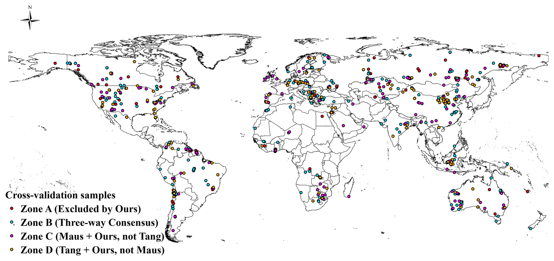
Figure A1Global spatial distribution of 750 cross-validation samples
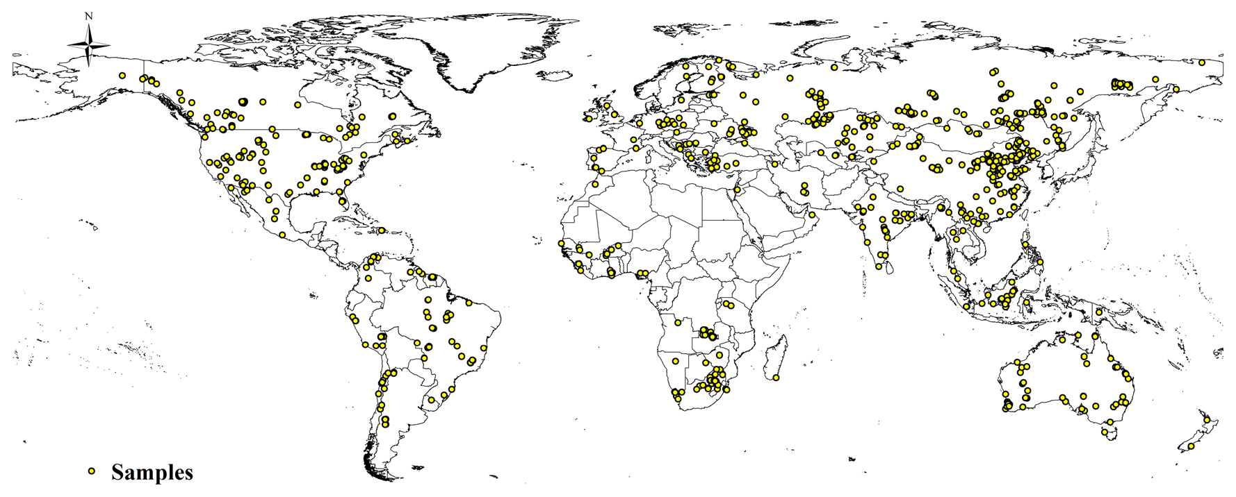
Figure A2Global spatial distribution of 1000 validation samples.
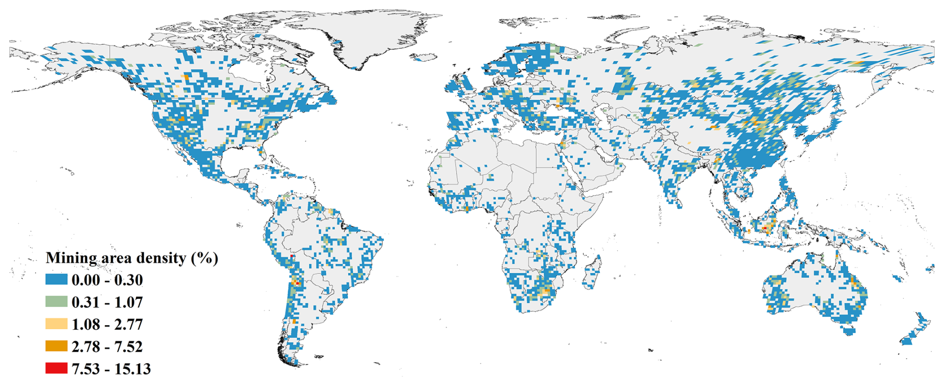
Figure A3Global mining density in a 100 km grid. Mining area density is calculated as the proportion of mining area within 100 × 100 km (10 000 km2) grid cells. Data was aggregated using the Interrupted Goode Homolosine equal-area projection to ensure accurate area calculations. The map is displayed using the PlateCarree projection.
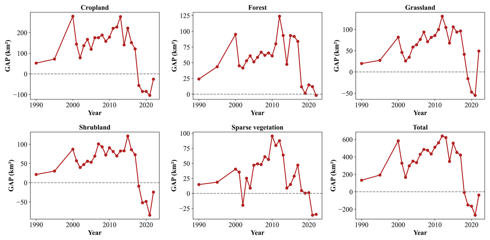
Figure A4Annual gap between damaged and reclaimed areas for five land cover types and total land (calculated every five years before 2000).
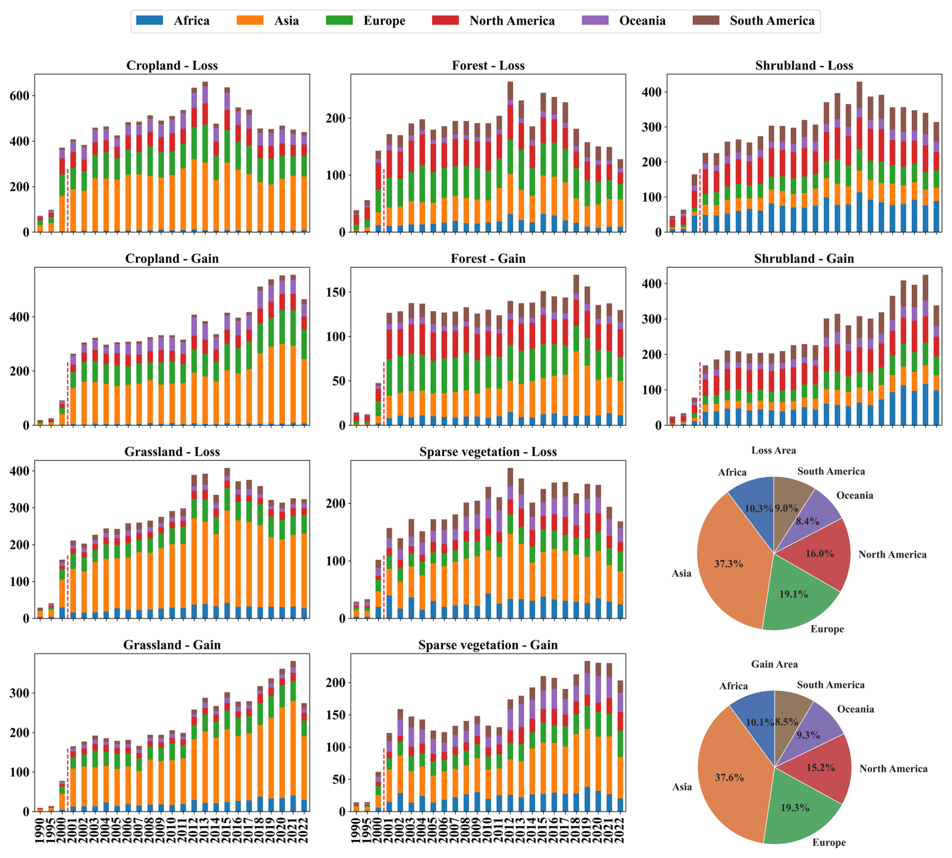
Figure A5Annual reclamation and damage of five land cover types across continents. To ensure the continuity of the graph, the values for 1990, 1995, and 2000 represent the average annual changes over five-year intervals.
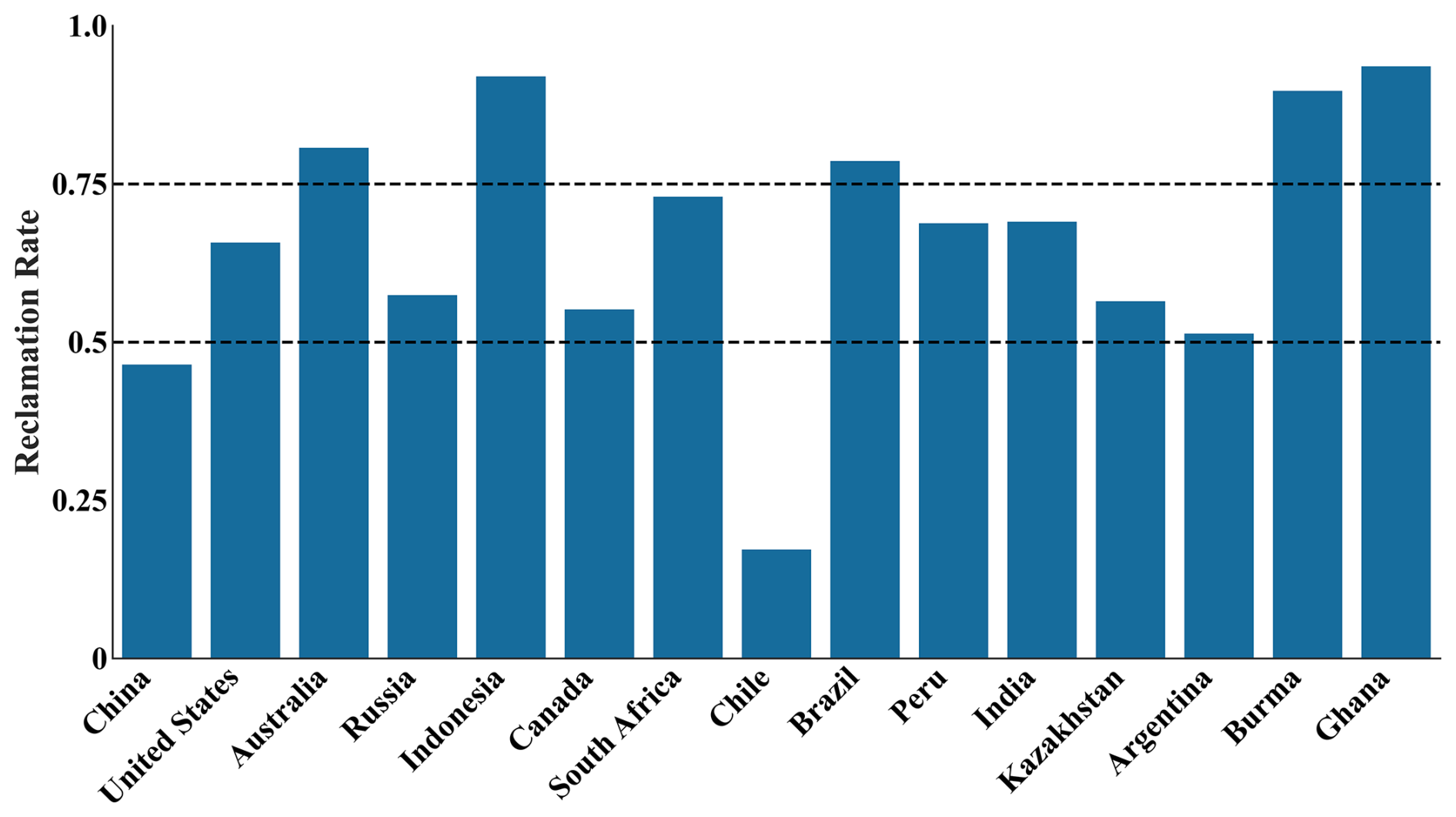
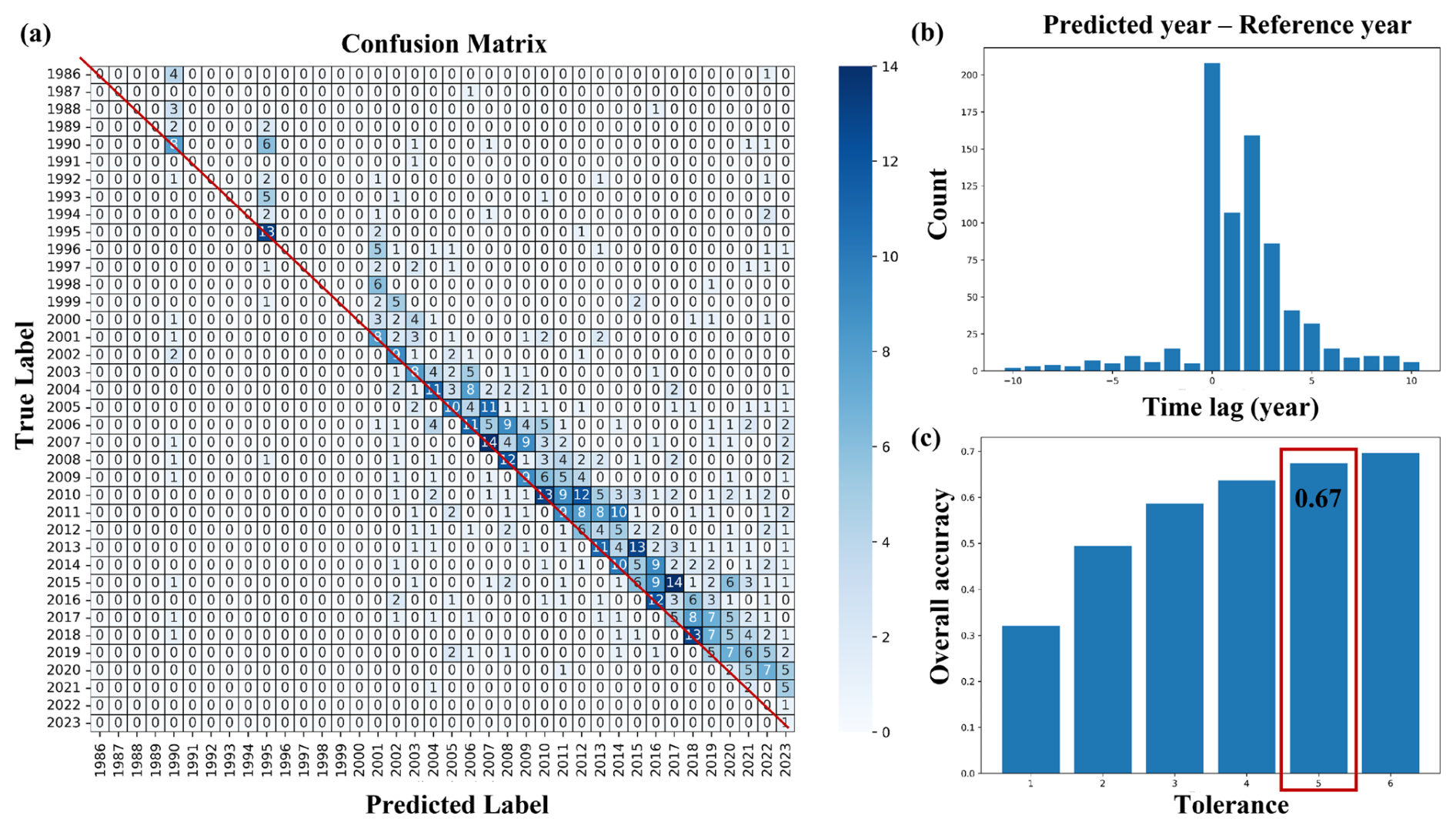
Figure A7Validation results. (a) Confusion matrix between predicted and reference change years; (b) Histogram of temporal lags between predicted and reference years; (c) Cumulative accuracy progression with increasing tolerance thresholds, validating the robustness of the ±5-year criterion.
Table A1Summary of per-country mine areas mapped in this study.
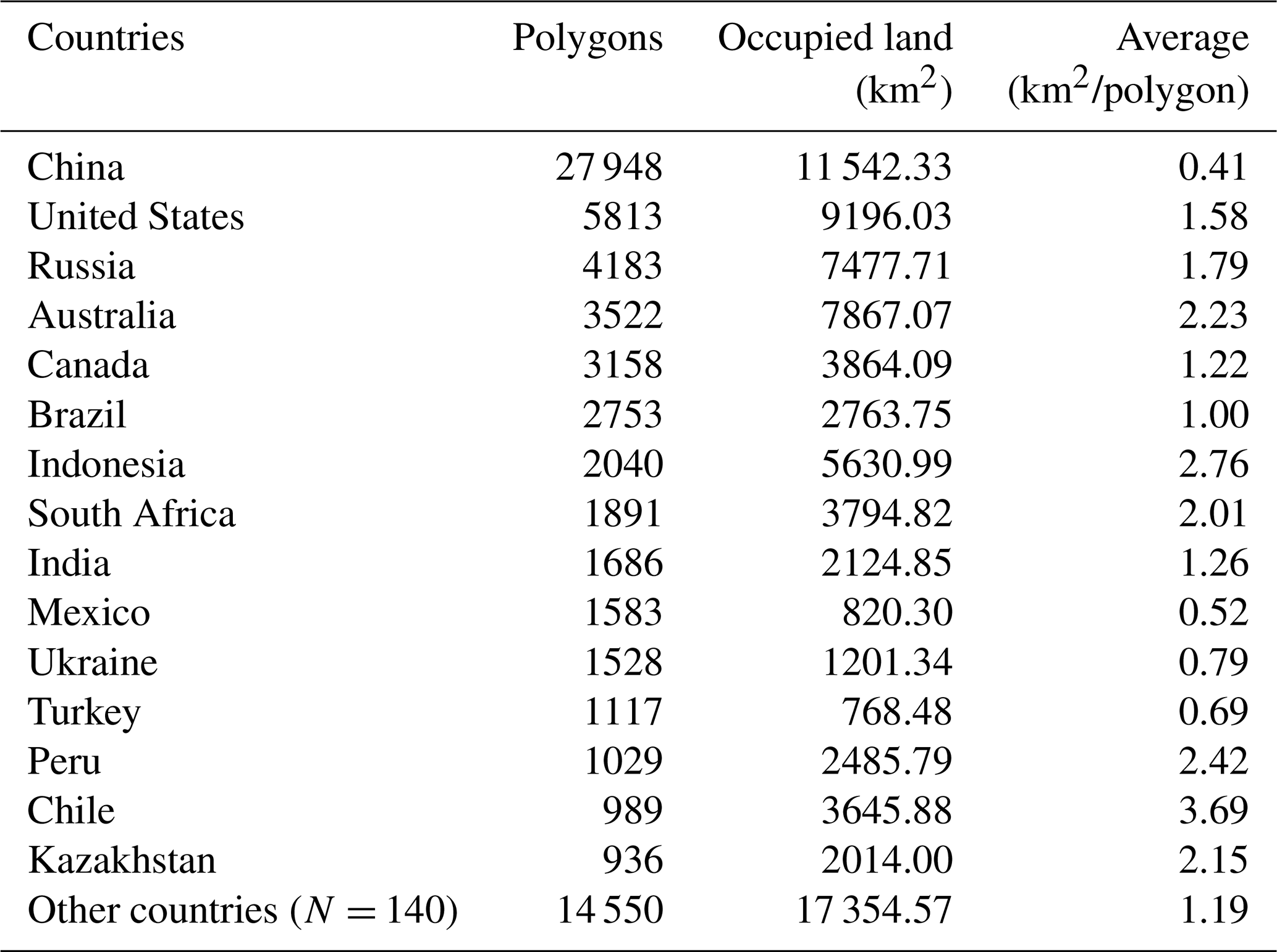
Table A2Summary of per-country mine areas within KBAs mapped in this study.
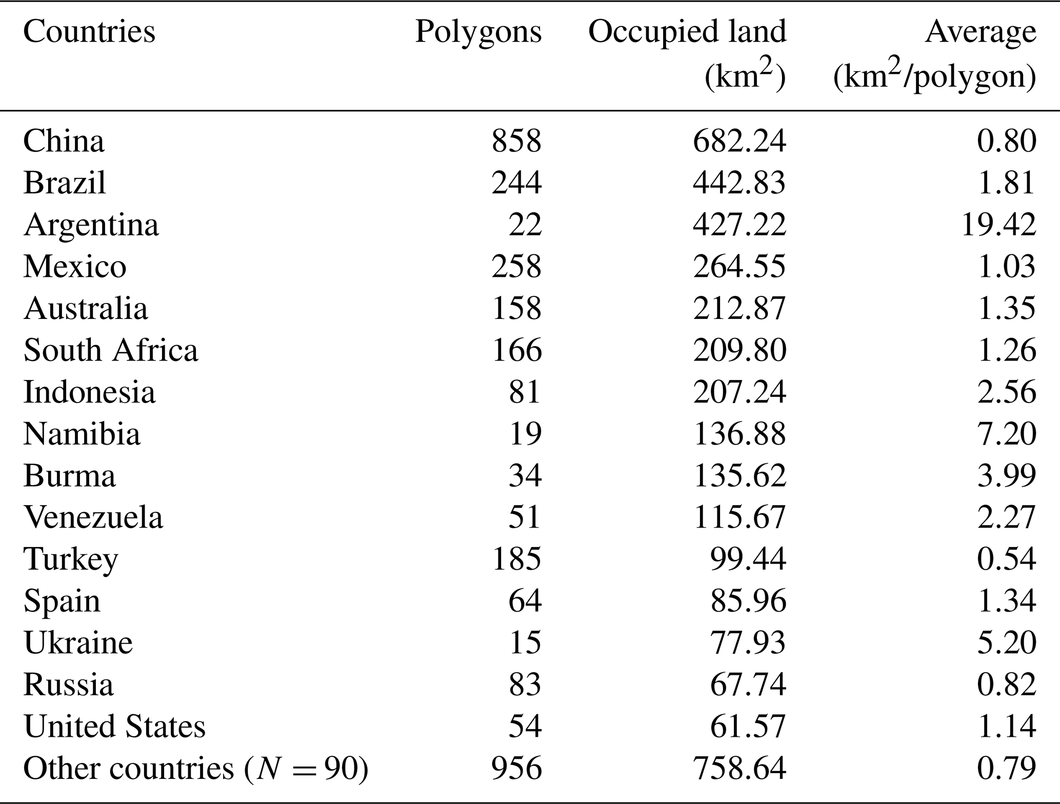
Table A3Distribution and accuracy rate of validation samples across global biomes.
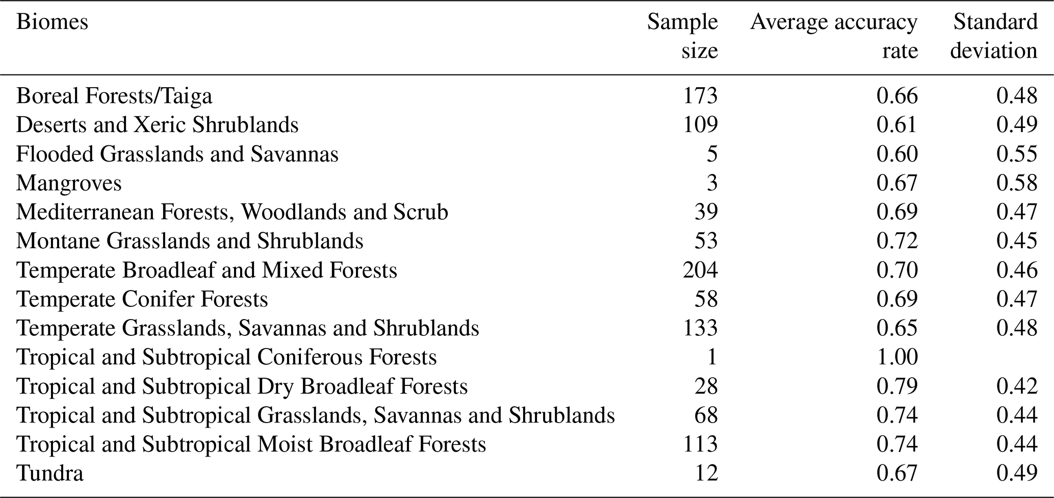
WX, SX, and JZ designed the research; SX and JZ developed the methodology, processed the data, and performed the analysis; KW and JG contributed to data Curation and visualization; SX and JZ wrote the original draft, which was supervised and critically revised by WX. SG, VM, TTW, and LT revised the draft; All authors contributed to the review and editing of the final manuscript.
The contact author has declared that none of the authors has any competing interests.
Publisher's note: Copernicus Publications remains neutral with regard to jurisdictional claims made in the text, published maps, institutional affiliations, or any other geographical representation in this paper. The authors bear the ultimate responsibility for providing appropriate place names. Views expressed in the text are those of the authors and do not necessarily reflect the views of the publisher.
This research has been supported by the National Key Research and Development Program of China (grant no. 2023YFE0122300) and the National Natural Science Foundation of China (grant no. 52674245).
This paper was edited by Han Ma and reviewed by Chu Zou and two anonymous referees.
Abbas, S., Saqib, N., and Shahzad, U.: Global export flow of chilean copper: The role of environmental innovation and renewable energy transition, Geosci. Front., 15, 101697, https://doi.org/10.1016/j.gsf.2023.101697, 2024.
Badgley, G., Field, C. B., and Berry, J. A.: Canopy near-infrared reflectance and terrestrial photosynthesis, Sci. Adv., 3, e1602244, https://doi.org/10.1126/sciadv.1602244, 2017.
Badgley, G., Anderegg, L. D. L., Berry, J. A., and Field, C. B.: Terrestrial gross primary production: Using NIRV to scale from site to globe, Glob. Change Biol., 25, 3731–3740, https://doi.org/10.1111/gcb.14729, 2019.
Boldy, R., Santini, T., Annandale, M., Erskine, P. D., and Sonter, L. J.: Understanding the impacts of mining on ecosystem services through a systematic review, The Extractive Industries and Society, 8, 457–466, https://doi.org/10.1016/j.exis.2020.12.005, 2021.
Carr-Wilson, S., Pattanayak, S. K., and Weinthal, E.: Critical mineral mining in the energy transition: A systematic review of environmental, social, and governance risks and opportunities, Energy Research & Social Science, 116, 103672, https://doi.org/10.1016/j.erss.2024.103672, 2024.
Chen, F., Zhu, Y., Bi, Y., Yang, Y., Ma, J., and Peng, S.: High-priority actions to improve carbon sequestration potential for mining ecological restoration in China, Engineering, 47, 16–21, https://doi.org/10.1016/j.eng.2024.09.012, 2025a.
Chen, W., Chen, L., Wei, Y., Ruan, L., Fu, Y., Li, W., He, T., and Xiao, W.: Using the forel-ule index (FUI) to track the water quality of subsidence water bodies across the life cycle of coal mining in eastern China, J. Environ. Manage., 374, 124037, https://doi.org/10.1016/j.jenvman.2025.124037, 2025b.
Cook-Patton, S. C., Leavitt, S. M., Gibbs, D., Harris, N. L., Lister, K., Anderson-Teixeira, K. J., Briggs, R. D., Chazdon, R. L., Crowther, T. W., Ellis, P. W., Griscom, H. P., Herrmann, V., Holl, K. D., Houghton, R. A., Larrosa, C., Lomax, G., Lucas, R., Madsen, P., Malhi, Y., Paquette, A., Parker, J. D., Paul, K., Routh, D., Roxburgh, S., Saatchi, S., van den Hoogen, J., Walker, W. S., Wheeler, C. E., Wood, S. A., Xu, L., and Griscom, B. W.: Mapping carbon accumulation potential from global natural forest regrowth, Nature, 585, 545–550, https://doi.org/10.1038/s41586-020-2686-x, 2020.
Feng, Y., Zeng, Z., Searchinger, T. D., Ziegler, A. D., Wu, J., Wang, D., He, X., Elsen, P. R., Ciais, P., Xu, R., Guo, Z., Peng, L., Tao, Y., Spracklen, D. V., Holden, J., Liu, X., Zheng, Y., Xu, P., Chen, J., Jiang, X., Song, X.-P., Lakshmi, V., Wood, E. F., and Zheng, C.: Doubling of annual forest carbon loss over the tropics during the early twenty-first century, Nat. Sustain., 5, 444–451, https://doi.org/10.1038/s41893-022-00854-3, 2022.
Firozjaei, M. K., Sedighi, A., Firozjaei, H. K., Kiavarz, M., Homaee, M., Arsanjani, J. J., Makki, M., Naimi, B., and Alavipanah, S. K.: A historical and future impact assessment of mining activities on surface biophysical characteristics change: A remote sensing-based approach, Ecol. Indic., 122, 107264, https://doi.org/10.1016/j.ecolind.2020.107264, 2021.
Giam, X., Olden, J. D., and Simberloff, D.: Impact of coal mining on stream biodiversity in the US and its regulatory implications, Nat. Sustain., 1, 176–183, https://doi.org/10.1038/s41893-018-0048-6, 2018.
Giljum, S., Maus, V., Kuschnig, N., Luckeneder, S., Tost, M., Sonter, L. J., and Bebbington, A. J.: A pantropical assessment of deforestation caused by industrial mining, P. Natl. Acad. Sci. USA, 119, e2118273119, https://doi.org/10.1073/pnas.2118273119, 2022.
Giljum, S., Maus, V., Sonter, L., Luckeneder, S., Werner, T., Lutter, S., Gershenzon, J., Cole, M. J., Siqueira-Gay, J., and Bebbington, A.: Metal mining is a global driver of environmental change, Nat. Rev. Earth Environ., 6, 441–455, https://doi.org/10.1038/s43017-025-00683-w, 2025.
Gorelick, N., Yang, Z., Arévalo, P., Bullock, E. L., Insfrán, K. P., and Healey, S. P.: A global time series dataset to facilitate forest greenhouse gas reporting, Environ. Res. Lett., 18, 084001, https://doi.org/10.1088/1748-9326/ace2da, 2023.
He, T., Zhang, M., Guo, A., Zhai, G., Wu, C., and Xiao, W.: A novel index combining temperature and vegetation conditions for monitoring surface mining disturbance using landsat time series, CATENA, 229, 107235, https://doi.org/10.1016/j.catena.2023.107235, 2023.
Hilson, G., Hilson, A., Maconachie, R., McQuilken, J., and Goumandakoye, H.: Artisanal and small-scale mining (ASM) in sub-Saharan Africa: Re-conceptualizing formalization and “illegal” activity, Geoforum, 83, 80–90, https://doi.org/10.1016/j.geoforum.2017.05.004, 2017.
Jacquin, A., Sheeren, D., and Lacombe, J.-P.: Vegetation cover degradation assessment in madagascar savanna based on trend analysis of MODIS NDVI time series, Int. J. Appl. Earth Obs., 12, S3–S10, https://doi.org/10.1016/j.jag.2009.11.004, 2010.
Jiang, Y., Liu, S., Liu, M., Peng, X., Liao, X., Wang, Z., and Gao, H.: A systematic framework for continuous monitoring of land use and vegetation dynamics in multiple heterogeneous mine sites, Remote Sens. Ecol. Conserv., 8, 793–807, https://doi.org/10.1002/rse2.276, 2022a.
Jiang, Y., Liu, S., Liu, M., Peng, X., Liao, X., Wang, Z., and Gao, H.: A systematic framework for continuous monitoring of land use and vegetation dynamics in multiple heterogeneous mine sites, Remote Sens. Ecol. Conserv., 8, 793–807, https://doi.org/10.1002/rse2.276, 2022b.
Karan, S. K., Samadder, S. R., and Maiti, S. K.: Assessment of the capability of remote sensing and GIS techniques for monitoring reclamation success in coal mine degraded lands, J. Environ. Manage., 182, 272–283, https://doi.org/10.1016/j.jenvman.2016.07.070, 2016.
Kennedy, R. E., Yang, Z., and Cohen, W. B.: Detecting trends in forest disturbance and recovery using yearly landsat time series: 1. LandTrendr – temporal segmentation algorithms, Remote Sens. Environ., 114, 2897–2910, https://doi.org/10.1016/j.rse.2010.07.008, 2010.
Ladewig, M., Angelsen, A., Masolele, R. N., and Chervier, C.: Deforestation triggered by artisanal mining in eastern Democratic Republic of the Congo, Nat. Sustain., 7, 1452–1460, https://doi.org/10.1038/s41893-024-01421-8, 2024.
Li, H., Wang, P., Werner, T. T., Chen, B., and Chen, W.-Q.: Machine learning-enhanced monitoring of global copper mining areas, Sci. Data, 12, 1120, https://doi.org/10.1038/s41597-025-05296-y, 2025.
Li, S., Xiao, W., Zhao, Y., and Lv, X.: Incorporating ecological risk index in the multi-process MCRE model to optimize the ecological security pattern in a semi-arid area with intensive coal mining: A case study in northern China, J. Clean. Prod., 247, 119143, https://doi.org/10.1016/j.jclepro.2019.119143, 2020.
Liang, T., Werner, T. T., Heping, X., Jingsong, Y., and Zeming, S.: A global-scale spatial assessment and geodatabase of mine areas, Global Planet. Change, 204, 103578, https://doi.org/10.1016/j.gloplacha.2021.103578, 2021.
Lv, X., Xiao, W., Zhao, Y., Zhang, W., Li, S., and Sun, H.: Drivers of spatio-temporal ecological vulnerability in an arid, coal mining region in western China, Ecol. Indic., 106, 105475, https://doi.org/10.1016/j.ecolind.2019.105475, 2019.
Ma, Q., Wu, J., He, C., and Fang, X.: The speed, scale, and environmental and economic impacts of surface coal mining in the Mongolian Plateau, Resour. Conserv. Recy., 173, 105730, https://doi.org/10.1016/j.resconrec.2021.105730, 2021.
Maus, V. and Werner, T. T.: Impacts for half of the world's mining areas are undocumented, Nature, 625, 26–29, https://doi.org/10.1038/d41586-023-04090-3, 2024.
Maus, V., Giljum, S., Gutschlhofer, J., Da Silva, D. M., Probst, M., Gass, S. L. B., Luckeneder, S., Lieber, M., and McCallum, I.: A global-scale data set of mining areas, Sci. Data, 7, 289, https://doi.org/10.1038/s41597-020-00624-w, 2020.
Maus, V., Giljum, S., da Silva, D. M., Gutschlhofer, J., da Rosa, R. P., Luckeneder, S., Gass, S. L. B., Lieber, M., and McCallum, I.: An update on global mining land use, Sci. Data, 9, 433, https://doi.org/10.1038/s41597-022-01547-4, 2022.
McKenna, P. B., Lechner, A. M., Phinn, S., and Erskine, P. D.: Remote sensing of mine site rehabilitation for ecological outcomes: A global systematic review, Remote Sens., 12, 3535, https://doi.org/10.3390/rs12213535, 2020.
Mi, J., Yang, Y., Zhang, S., An, S., Hou, H., Hua, Y., and Chen, F.: Tracking the Land Use/Land Cover Change in an Area with Underground Mining and Reforestation via Continuous Landsat Classification, Remote Sens., 11, 1719, https://doi.org/10.3390/rs11141719, 2019.
Murguía, D. I. and Bringezu, S.: Measuring the specific land requirements of large-scale metal mines for iron, bauxite, copper, gold and silver, PIE, 10, 264, https://doi.org/10.1504/PIE.2016.082142, 2016.
Olson, D. M., Dinerstein, E., Wikramanayake, E. D., Burgess, N. D., Powell, G. V. N., Underwood, E. C., D'amico, J. A., Itoua, I., Strand, H. E., Morrison, J. C., Loucks, C. J., Allnutt, T. F., Ricketts, T. H., Kura, Y., Lamoreux, J. F., Wettengel, W. W., Hedao, P., and Kassem, K. R.: Terrestrial ecoregions of the world: A new map of life on earth: a new global map of terrestrial ecoregions provides an innovative tool for conserving biodiversity, BioScience, 51, 933–938, https://doi.org/10.1641/0006-3568(2001)051[0933:TEOTWA]2.0.CO;2, 2001.
Oramah, I. T., Richards, J. P., Summers, R., Garvin, T., and McGee, T.: Artisanal and small-scale mining in Nigeria: Experiences from Niger, Nasarawa and Plateau states, The Extractive Industries and Society, 2, 694–703, https://doi.org/10.1016/j.exis.2015.08.009, 2015.
Pavloudakis, F., Roumpos, C., and Spanidis, P.-M.: Sustainable Mining and Processing of Mineral Resources, Sustainability, 16, 8393, https://doi.org/10.3390/su16198393, 2024.
Poorter, L., Craven, D., Jakovac, C. C., van der Sande, M. T., Amissah, L., Bongers, F., Chazdon, R. L., Farrior, C. E., Kambach, S., Meave, J. A., Muñoz, R., Norden, N., Rüger, N., van Breugel, M., Almeyda Zambrano, A. M., Amani, B., Andrade, J. L., Brancalion, P. H. S., Broadbent, E. N., de Foresta, H., Dent, D. H., Derroire, G., DeWalt, S. J., Dupuy, J. M., Durán, S. M., Fantini, A. C., Finegan, B., Hernández-Jaramillo, A., Hernández-Stefanoni, J. L., Hietz, P., Junqueira, A. B., N'dja, J. K., Letcher, S. G., Lohbeck, M., López-Camacho, R., Martínez-Ramos, M., Melo, F. P. L., Mora, F., Müller, S. C., N'Guessan, A. E., Oberleitner, F., Ortiz-Malavassi, E., Pérez-García, E. A., Pinho, B. X., Piotto, D., Powers, J. S., Rodríguez-Buriticá, S., Rozendaal, D. M. A., Ruíz, J., Tabarelli, M., Teixeira, H. M., Valadares de Sá Barretto Sampaio, E., van der Wal, H., Villa, P. M., Fernandes, G. W., Santos, B. A., Aguilar-Cano, J., de Almeida-Cortez, J. S., Alvarez-Davila, E., Arreola-Villa, F., Balvanera, P., Becknell, J. M., Cabral, G. A. L., Castellanos-Castro, C., de Jong, B. H. J., Nieto, J. E., Espírito-Santo, M. M., Fandino, M. C., García, H., García-Villalobos, D., Hall, J. S., Idárraga, A., Jiménez-Montoya, J., Kennard, D., Marín-Spiotta, E., Mesquita, R., Nunes, Y. R. F., Ochoa-Gaona, S., Peña-Claros, M., Pérez-Cárdenas, N., Rodríguez-Velázquez, J., Villanueva, L. S., Schwartz, N. B., Steininger, M. K., Veloso, M. D. M., Vester, H. F. M., Vieira, I. C. G., Williamson, G. B., Zanini, K., and Hérault, B.: Multidimensional tropical forest recovery, Science, 374, 1370–1376, https://doi.org/10.1126/science.abh3629, 2021.
Qian, D., Yan, C., Xiu, L., and Feng, K.: The impact of mining changes on surrounding lands and ecosystem service value in the Southern Slope of Qilian Mountains, Ecol. Complex., 36, 138–148, https://doi.org/10.1016/j.ecocom.2018.08.002, 2018.
Ross, M. L. and Werker, E.: Diversification in resource-rich africa, 1999–2019, Resour. Policy, 88, 104437, https://doi.org/10.1016/j.resourpol.2023.104437, 2024.
Schandl, H., Marcos-Martinez, R., West, J., Miatto, A., Lutter, S., Lieber, M., Giljum, S., Lenzen, M., Li, M., Wang, H., Tanikawa, H., Krausmann, F., Eisenmenger, N., and Fischer-Kowalski, M.: Global material flows and resource productivity: The 2024 update, J. Indust. Ecol., 28, 2012–2031, https://doi.org/10.1111/jiec.13593, 2024.
Sepin, P., Vashold, L., and Kuschnig, N.: Mapping mining areas in the tropics from 2016 to 2024, Nat. Sustain., 8, 1400–1407, https://doi.org/10.1038/s41893-025-01668-9, 2025.
Sonter, L. J., Herrera, D., Barrett, D. J., Galford, G. L., Moran, C. J., and Soares-Filho, B. S.: Mining drives extensive deforestation in the Brazilian Amazon, Nat. Commun., 8, 1013, https://doi.org/10.1038/s41467-017-00557-w, 2017.
Sonter, L. J., Ali, S. H., and Watson, J. E. M.: Mining and biodiversity: Key issues and research needs in conservation science, P. Roy. Soc. B., 285, https://doi.org/10.1098/rspb.2018.1926, 2018.
Sonter, L. J., Nursamsi, I., Bennun, L., Graham, J., Maus, V., Rainey, H., Starkey, M., Turner, J. A., Watson, J. E. M., and Prescott, G. W.: Global land cover maps do not reveal mining pressures to biodiversity, Sci. Rep., 15, 22421, https://doi.org/10.1038/s41598-025-01959-3, 2025.
Tai, X., Xiao, W., and Tang, Y.: A quantitative assessment of vulnerability using social-economic-natural compound ecosystem framework in coal mining cities, J. Clean. Prod., 258, 120969, https://doi.org/10.1016/j.jclepro.2020.120969, 2020.
Tang, L. and Werner, T. T.: Global mining footprint mapped from high-resolution satellite imagery, Commun. Earth Environ., 4, 134, https://doi.org/10.1038/s43247-023-00805-6, 2023.
Wang, K., Zhou, J., Yang, R., Xu, S., Hu, Z., and Xiao, W.: Deploying photovoltaic systems in global open-pit mines for a clean energy transition, Nat. Sustain., 8, 1037–1047, https://doi.org/10.1038/s41893-025-01594-w, 2025.
Werner, T. T., Bebbington, A., and Gregory, G.: Assessing impacts of mining: Recent contributions from GIS and remote sensing, The Extractive Industries and Society, 6, 993–1012, https://doi.org/10.1016/j.exis.2019.06.011, 2019.
Werner, T. T., Mudd, G. M., Schipper, A. M., Huijbregts, M. A. J., Taneja, L., and Northey, S. A.: Global-scale remote sensing of mine areas and analysis of factors explaining their extent, Global Environ. Chang., 60, 102007, https://doi.org/10.1016/j.gloenvcha.2019.102007, 2020.
Xiang, H., Wang, Z., Mao, D., Zhang, J., Zhao, D., Zeng, Y., and Wu, B.: Surface mining caused multiple ecosystem service losses in China, J. Environ. Manage., 290, 112618, https://doi.org/10.1016/j.jenvman.2021.112618, 2021.
Xiao, W., Lv, X., Zhao, Y., Sun, H., and Li, J.: Ecological resilience assessment of an arid coal mining area using index of entropy and linear weighted analysis: A case study of shendong coalfield, China, Ecol. Indic., 109, 105843, https://doi.org/10.1016/j.ecolind.2019.105843, 2020a.
Xiao, W., Deng, X., He, T., and Chen, W.: Mapping annual land disturbance and reclamation in a surface coal mining region using google earth engine and the LandTrendr algorithm: A case study of the shengli coalfield in inner mongolia, China, Remote Sens., 12, 1612, https://doi.org/10.3390/rs12101612, 2020b.
Xiao, W., Deng, X., He, T., and Chen, W.: Mapping annual land disturbance and reclamation in a surface coal mining region using google earth engine and the LandTrendr algorithm: A case study of the shengli coalfield in inner mongolia, China, Remote Sens., 12, 1612, https://doi.org/10.3390/rs12101612, 2020c.
Xu, H., Xu, F., Lin, T., Xu, Q., Yu, P., Wang, C., Aili, A., Zhao, X., Zhao, W., Zhang, P., Yang, Y., and Yuan, K.: A systematic review and comprehensive analysis on ecological restoration of mining areas in the arid region of China: Challenge, capability and reconsideration, Ecol. Indic., 154, 110630, https://doi.org/10.1016/j.ecolind.2023.110630, 2023.
Xu, S., Zhou, J., and Xiao, W.: Global surface mining and land reclamation of time series from 1985–2022, Zenodo [data set], https://doi.org/10.5281/zenodo.17085099, 2025.
Xu, S., Zhou, J., and Xiao, W.: GlobalMiningDatabase v1.0.0, Zenodo [code], https://doi.org/10.5281/zenodo.21293825, 2026.
Yan, X., Li, J., Shao, Y., Ma, T., Zhang, R., and Su, Y.: Assessing open-pit mining impacts on semi-arid grassland: A framework for boundary and intensity quantification, J. Clean. Prod., 475, 143464, https://doi.org/10.1016/j.jclepro.2024.143464, 2024.
Yang, J. and Huang, X.: The 30 m annual land cover dataset and its dynamics in China from 1990 to 2019, Earth Syst. Sci. Data, 13, 3907–3925, https://doi.org/10.5194/essd-13-3907-2021, 2021.
Yang, Y., Erskine, P. D., Lechner, A. M., Mulligan, D., Zhang, S., and Wang, Z.: Detecting the dynamics of vegetation disturbance and recovery in surface mining area via landsat imagery and LandTrendr algorithm, J. Clean. Prod., 178, 353–362, https://doi.org/10.1016/j.jclepro.2018.01.050, 2018.
Yu, L., Xu, Y., Xue, Y., Li, X., Cheng, Y., Liu, X., Porwal, A., Holden, E.-J., Yang, J., and Gong, P.: Monitoring surface mining belts using multiple remote sensing datasets: A global perspective, Ore Geol. Rev., 101, 675–687, https://doi.org/10.1016/j.oregeorev.2018.08.019, 2018.
Zhang, X., Zhao, T., Xu, H., Liu, W., Wang, J., Chen, X., and Liu, L.: GLC_FCS30D: the first global 30 m land-cover dynamics monitoring product with a fine classification system for the period from 1985 to 2022 generated using dense-time-series Landsat imagery and the continuous change-detection method, Earth Syst. Sci. Data, 16, 1353–1381, https://doi.org/10.5194/essd-16-1353-2024, 2024.
Zhao, Y., Wang, Y., Zhang, Z., Zhou, Y., Huang, H., and Chang, M.: The Evolution of Landscape Patterns and Its Ecological Effects of Open-Pit Mining: A Case Study in the Heidaigou Mining Area, China, Int. J. Env. Res. Pub. He., 20, 4394, https://doi.org/10.3390/ijerph20054394, 2023.
Zhu, Z. and Woodcock, C. E.: Continuous change detection and classification of land cover using all available Landsat data, Remote Sens. Environ., 144, 152–171, https://doi.org/10.1016/j.rse.2014.01.011, 2014.