Multi-year observations of BVOCs and ozone: concentrations and fluxes measured above and below the canopy in a mixed temperate forest

Volatile organic compounds (VOCs) and ozone (O₃) are key constituents of tropospheric chemistry, affecting both air quality and climate. Forests are major emitters of biogenic VOCs (BVOCs), yet large uncertainties remain regarding the diversity of exchanged compounds, the drivers of their bidirectional fluxes, and their in-canopy chemistry. Long-term and comprehensive in situ datasets remain scarce, limiting our understanding of these complex processes. We conducted a 3-year field campaign (2022–2024) at the Integrated Carbon Observation System mixed temperate forest station of Vielsalm (BE-Vie), combining vertical concentration profile and eddy covariance flux measurements above and below the canopy (concentration dataset: https://doi.org/10.18758/NVFBA74V, Verreyken et al., 2025c; flux dataset: https://doi.org/10.18758/KHV8ZXU2, Dumont et al., 2025a; concentration-turbulence profile dataset: https://doi.org/10.18758/BED4Q2VY, Dumont et al., 2025b). Using a PTR-ToF-MS and an open-source data-processing workflow, we identified 48 significantly exchanged VOCs. The vertical and diurnal gradients of the mixing ratios reflected the interplay between emission, deposition, chemistry, and transport. Combined with a profile of turbulence statistics, these observations offer an opportunity to investigate their behaviour within the canopy. The forest acted as a net VOC source in summer (∼ 1.25 µg m⁻² s⁻¹), while deposition dominated in autumn. Many oxygenated VOCs displayed bidirectional exchange. Monoterpenes, isoprene, and methanol were the most abundant flux contributors, but 15–30 (30–43) compounds were needed to account for 90 % of total emissions (depositions), depending on the season. Below-canopy BVOC and O₃ fluxes reached ∼ 10 % of above-canopy ones, with proportionally enhanced below-canopy ozone uptake at night. This study provides one of the most detailed long-term datasets of VOC and O₃ exchange in a temperate forest and serves as a key reference for improving process-based models of biogenic, physical, and chemical exchange in forest ecosystems.

1 Introduction

Volatile organic compounds (VOCs) form a heterogeneous group of reactive trace gases that play a key role in atmospheric chemistry. Together with nitrogen oxides (NO_x), they contribute to both the formation and destruction of tropospheric ozone (Stockwell and Forkel, 2002), influencing regional ozone pollution. By reacting with hydroxyl and peroxy radicals, VOCs also affect the atmospheric oxidizing capacity and the lifetime of methane (Yoon et al., 2025), the second most important radiatively active gas after carbon dioxide (Canadell et al., 2021). In addition, VOCs are precursors in the formation and growth of secondary organic aerosols (SOA) (Mahilang et al., 2021), thereby degrading air quality, impacting human health, and influencing climate through interactions with radiation and serving as cloud condensation nuclei.

Each year, terrestrial ecosystems emit over 1000 Tg of organic carbon in the form of biogenic VOCs (BVOCs), excluding methane (Guenther et al., 2012). This exceeds global emissions of methane (∼ 550 Tg yr⁻¹) (Saunois et al., 2016) and anthropogenic VOCs (∼ 200 Tg yr⁻¹) (Huang et al., 2017). Forests are the dominant BVOC emitters among terrestrial ecosystems (Isidorov et al., 2022, and references therein), making them a longstanding focus of atmospheric research. Within forests, Guenther et al. (2012) estimated that broadleaf deciduous temperate trees rank third in isoprene emissions, contributing 35.4 Tg yr⁻¹, compared to 244 and 178 Tg yr⁻¹ for tropical evergreen and deciduous forests, respectively. Similarly, needleleaf evergreen temperate trees are the third largest monoterpene emitters, with 7.38 Tg yr⁻¹, behind tropical evergreen and deciduous forests (82.9 and 45 Tg yr⁻¹, respectively). These estimates suggest that temperate forests composed of mixed deciduous and needleleaf species deserve particular attention.

Ozone (O₃), in addition to its role in radiative forcing as a potent greenhouse gas (Rowlinson et al., 2020), is toxic to both humans and plants. In terrestrial ecosystems, it undergoes various dry deposition pathways – including stomatal and non-stomatal processes such as uptake by leaf cuticles, soil, snow, or water surfaces (Clifton et al., 2020). Ozone deposition contributes significantly to reducing tropospheric ozone levels. However, when ozone enters leaves through stomata, it generates reactive oxygen species (ROS), which can damage plant cells, accelerate senescence, and reduce carbon assimilation via photosynthesis (Fiscus et al., 2005).

Despite decades of research into ozone uptake partitioning (Padro, 1996; Cieslik, 1998; Lamaud et al., 2002; Zhang et al., 2002; Mikkelsen et al., 2004; Fares et al., 2014; Horváth et al., 2017; Zhou et al., 2017b; Finco et al., 2018; Gerosa et al., 2022b), significant uncertainties remain. One such uncertainty lies in the reactions of ozone with BVOCs, which constitute an increasingly recognized atmospheric sink (Clifton et al., 2020, and references therein). This process, however, remains highly variable and difficult to quantify (Kurpius and Goldstein, 2003; Goldstein et al., 2004; Wolfe et al., 2011; Vermeuel et al., 2021).

Unlike ozone, BVOCs can undergo both emission and deposition. Early research primarily focused on isoprene and monoterpenes – the two most widely emitted isoprenoids globally (Guenther et al., 2012) – whose fluxes were long considered exclusively upward, with isoprene emissions driven by light and temperature and monoterpene emissions by temperature alone (Guenther et al., 1995). Later studies extended global emission inventories to include oxygenated VOCs (OVOCs, e.g., methanol, ethanol, acetone, acetaldehyde, formaldehyde, formic and acetic acids), sesquiterpenes, and isoprenoid oxidation products (Niinemets et al., 2014; Guenther et al., 2012), but largely continued to focus on emissions rather than deposition. Yet, in situ studies have highlighted non-negligible deposition fluxes of BVOCs (Karl et al., 2010; Bamberger et al., 2011; Jardine et al., 2011; Ruuskanen et al., 2011; Laffineur et al., 2012; Park et al., 2013a; Nguyen et al., 2015; Wohlfahrt et al., 2015; Zhou et al., 2017b), which are now recognized as significant in global budgets. For instance, Safieddine et al. (2017) estimated that 460 Tg C yr⁻¹ of reactive organic carbon is removed from the atmosphere via physical deposition. A regional simulation over the U.S. further showed that dry and wet deposition of organic vapours accounted for 60 %–75 % of the removal of tropospheric SOA burden in summer 2010 by limiting the availability of SOA precursors (Hodzic et al., 2014).

It is now well established that many BVOCs undergo bidirectional exchange. Yet, emissions and depositions are generally modelled separately in chemical transport models (CTMs), despite being driven by similar environmental variables (Forkel et al., 2015). Emissions are often simulated using the MEGAN model (for example, Sindelarova et al., 2014; Opacka et al., 2021; Wang et al., 2022; Zeng et al., 2023), one of the most widely used biogenic emission models, which combines species-specific emission potentials with responses to light, temperature, CO₂ inhibition, and leaf age (Guenther et al., 2012). Deposition, in contrast, is usually calculated as the product of ambient concentration and deposition velocity, using an Ohm’s law analogy introduced by Wesely (1989). This approach depends on deposition velocity estimates, which are still scarce, uncertain, and rarely incorporate seasonal variation (Niinemets et al., 2014). Other frameworks based on compensation points require precise knowledge of intercellular VOC concentrations and stomatal behaviour, and are difficult to upscale to the ecosystem level (Niinemets et al., 2014).

An additional process often overlooked in surface exchange models is in-canopy chemistry, which, in interaction with turbulent mixing, can significantly alter fluxes of highly reactive compounds such as sesquiterpenes (Forkel et al., 2015). VOCs can be lost between their point of release and the atmosphere above the canopy, where chemical processing depends strongly on turbulent mixing and residence times within the canopy (Rinne et al., 2007; Zhou et al., 2017b), affecting CTM predictions of atmospheric concentrations in ways that are not yet adequately represented (Vermeuel et al., 2024; Link et al., 2024). Accounting for these reactions also requires identifying the vertical distribution of sources and sinks within the canopy. Although several studies have applied inverse modelling to approach this question, few ecosystems and tracers have been characterized to date (Karl et al., 2004a; Tiwary et al., 2007; Wada et al., 2020; Petersen et al., 2023). Overall, there is a growing call for a unified framework to model bidirectional BVOC exchange, integrating altogether dry and wet deposition, direct emissions, and in-canopy chemistry (Pleim and Ran, 2011; Niinemets et al., 2014; Forkel et al., 2015).

While emission models such as MEGAN have become increasingly sophisticated, they still represent only a fraction of the chemical diversity of atmospheric VOCs. For example, MEGAN2.1 includes 147 compounds (Guenther et al., 2012), whereas most CTMs simulate only 30–45 species (Millet et al., 2018). This limited representation contrasts starkly with field observations: Goldstein and Galbally (2007) estimated that between 10⁴ and 10⁵ distinct organic compounds have been detected in the atmosphere. Flux measurements have also revealed remarkable chemical diversity, with over 500 VOC-related ions observed over an orange orchard (Park et al., 2013a) and 377 over a temperate forest (Millet et al., 2018).

Improving VOC exchange parametrizations requires in situ, ecosystem-scale flux measurements across a diversity of ecosystems and environmental conditions. Traditionally, such measurements relied on disjunct eddy covariance (Muller et al., 2010; Laffineur et al., 2011, 2012, 2013; Rinne et al., 2007; Yang et al., 2013; Seco et al., 2015; Bachy et al., 2016, 2018; Seco et al., 2017) and, more occasionally, on surface-layer gradient and profile methods (Rantala et al., 2014, and references therein), using PTR-Quad-MS instruments. Using this type of instrument allowed the monitoring of a limited number of pre-selected compounds and could not resolve isobaric interferences. As a consequence, this technique was mostly used to investigate well-known BVOCs (Schallhart et al., 2016). More recently, the advent of PTR-ToF-MS coupled with eddy covariance enabled the simultaneous detection of fluxes for hundreds of VOCs with improved sensitivity and mass resolution, allowing isobar separation (Ruuskanen et al., 2011; Kaser et al., 2013; Park et al., 2013a, b; Brilli et al., 2014, 2016; Schallhart et al., 2016; Juráň et al., 2017; Millet et al., 2018; Schallhart et al., 2018; Jensen et al., 2018; Fischer et al., 2021; Manco et al., 2021; Loubet et al., 2022; Petersen et al., 2023; Vermeuel et al., 2023b). However, many studies remained compound-targeted, and the technical complexity of PTR-ToF-MS operation and data processing limited their temporal coverage (Rinne et al., 2016). As a result, long-term flux measurements across seasons and under variable conditions remain scarce.

In this study, we revisit a temperate mixed forest in southern Belgium (Vielsalm station, BE-Vie), more than 10 years after the first PTR-Quad-MS flux measurements (Laffineur et al., 2011, 2012, 2013), with the aim of expanding the existing dataset. Using a PTR-ToF-MS and ozone analysers, we conducted a 3-year measurement campaign to obtain:

• i.

  1 min concentrations of BVOCs and O₃ above the canopy and at ground level,

• ii.

  30 min fluxes of BVOCs and O₃ above the canopy and at ground level,

• iii.

  vertical profiles of BVOC and O₃ concentrations at seven levels from the trunk space to above the canopy, and

• iv.

  vertical profiles of turbulence measured by sonic anemometers at eight levels.

We provide a detailed description of the VOC data processing workflow – including newly developed and openly available processing tools – from raw PTR-ToF-MS signal treatment to compound identification, quantification, flux calculation, and data flagging, following a non-targeted and comprehensive approach. Ozone flux data processing is also described in detail, and methodological issues raised in earlier studies (Muller et al., 2010; Zhu et al., 2015) are discussed.

To our knowledge, this study presents the longest combined VOC and ozone flux dataset publicly available to date, spanning 3 years and covering seasonal transitions from spring to summer and summer to autumn. Combined with additional open-access measurements at the site (extensive meteorological and phenological characterization, BTEX, HAPs, NO_x, fine particles, and aerosols), this structured database offers a unique opportunity to address key knowledge gaps. These include quantifying the magnitude and diversity of BVOC exchange in temperate forests, their influence on ozone levels, the dynamics of bidirectional fluxes, the spatial distribution of sources and sinks, and the role of in-canopy chemistry. As a result, it provides a strong basis for improving current parametrizations in surface exchange models and CTMs, and to advancing our understanding of VOC and ozone interactions in the Earth system.

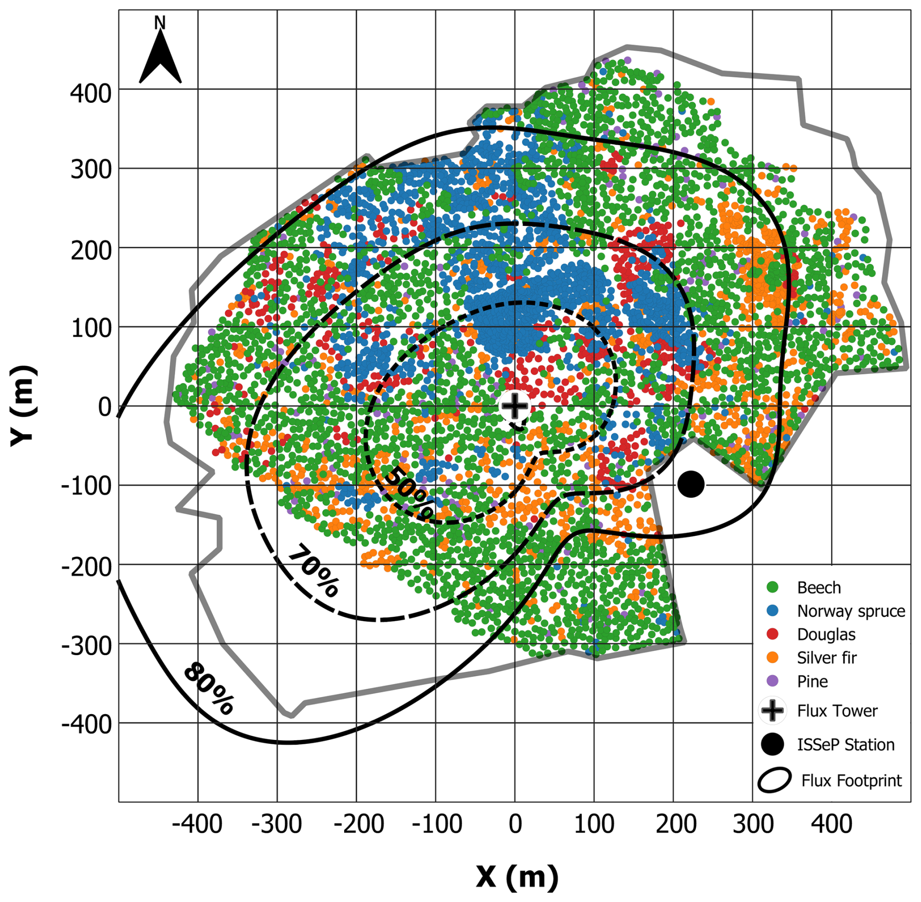
Figure 1 Map of the study site with details about (i) dominant tree distribution, (ii) footprint climatology (50 %, 70 % and 80 % isopleths) and (iii) research infrastructures (flux tower and ISSeP station). The grey line represents the border of the ICOS target area.

2 Material and methods

2.1 Study site

The study site (BE-Vie) is a mature mixed forest ecosystem, located in Vielsalm in the Belgian Ardenne region (50°18^′ N, 6°00^′ E; altitude 470 m a.s.l.). This site is part of several gas measurement networks: ICOS (class 2 ecosystem station) (https://www.icos-cp.eu/, last access: 13 January 2026), ACTRIS (for particle and gas in situ) (https://www.actris.eu/, last access: 13 January 2026), and EMEP (level 1 station) (https://www.emep.int/, last access: 13 January 2026). Its climate is temperate maritime and the 50-100 cm deep soil is classified as a dystric cambisol. The vegetation within the target area (that is, the area that contributes the most to fluxes measured at the flux tower) is a mixture of coniferous species, mainly Norway spruce (Picea abies [L.] Karst., mean height 17 m), Douglas fir (Pseudotsuga menziesii [Mirb.] Franco, 37 m) and Silver fir (Abies alba Miller, 26 m); and deciduous species, mainly European beech (Fagus sylvatica L., 22 m). Tree heights are reported from the last extensive inventory in the surroundings of the flux tower (2019), yielding an overall mean tree height of 26 m. Besides tree saplings, the understory vegetation is very sparse and is mainly composed of mosses (∼ 76 % of the understory vegetation in dry weight), shrubs (∼ 15 %, mainly Vaccinium myrtillus [L.] and Rubus species), and ferns (∼ 8 %). Figure 1 gives a distribution of dominant tree species in most of the target area. This classification is based on multispectral images acquired with a drone in 2018 (Lanssens, 2019). The dominant winds blow from the south-west (sector dominated by European beech) and the north-east (sector dominated by Norway spruce and Douglas fir). The footprint climatology was obtained using the model by Kljun et al. (2015) and is shown in Fig. 1. Within the 70 % cumulative footprint, the distribution of tree species is dominated by Norway spruce (38 %) and European beech (36 %), followed by Silver fir (14 %), Douglas fir (9 %), and Scots pine (2 %).

The study site is located in a rural area with low anthropogenic activity, except for a sawmill 3 km south-west of the flux tower and two small industrial hubs around 7 km north-east and south-east. ICOS-related measurements are carried out on the 51 m high flux tower and its close surroundings. Another measurement station, operated by the Walloon Scientific Institute for Public Service (ISSeP) – the regional environmental authority – is located in the same forest, approximately 250 m from the flux tower. Measurements carried out at the ISSeP station are detailed in Sect. 2.5.2. More information about the study site are available in Aubinet et al. (2001, 2018). Note that all times reported in this paper are given in local time (LT), defined as Central European Time (UTC+1) without daylight saving time (DST).

2.2 Experimental setup

Three setups were operated at BE-Vie from 2022 to 2024: the TOP system, the TRUNK system, and the PROFILE system. These are described below, and details about the related analytical techniques are provided in Sect. 2.3, while flux computations are discussed in Sects. 2.3.3 and 2.4.

2.2.1 TOP system

To characterize the bidirectional fluxes of BVOCs and O₃ above the canopy, a first setup was installed at the top of the 51 m high flux tower (level H7 in Fig. 2). Flux measurements were performed using the eddy covariance (EC) technique, which is based on fast measurements of the vertical wind velocity and the mixing ratio of the tracer of interest.

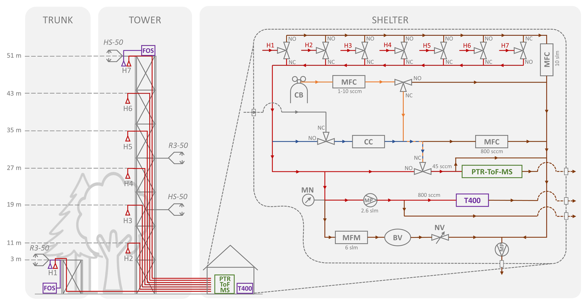
Figure 2 Schematic representation of the concentration and sonic anemometer profile setup, including a zoom on the pneumatical system. Instruments include: FOS – fast ozone analyser; T400 – slow ozone analyser; PTR-ToF-MS – fast VOC analyser; HS-50 & R3–50 – sonic anemometers; CB – calibration bottle; MFC – mass flow controller; CC – catalytic converter; MN – manometer; MP – membrane pump; MFM – mass flow meter; BV – buffer volume; NV – needle valve. Line colours indicate function: purple – ozone line, red – ozone/VOC line, blue – background line, orange – calibration line, brown – exhaust line. The positions of the solenoid valves are indicated by NO (normally open, i.e. open without electrical activation) and NC (normally closed, i.e. open only when electrically activated).

At the top of the tower, a 3D HS-50 sonic anemometer (Gill Instrument Ltd, UK) was used to record 3D wind components at a frequency of 10 Hz (see Table 1 for a summary of the instruments used). To measure BVOC and O₃ mixing ratios, ambient air was sampled at level H7 close to the HS-50 measurement volume and pumped to a wooden shelter at ground level through a 60 m long and 6.4 mm inner-diameter PFA (perfluoroalkoxy alkane) tubing (Fluortechnik-Deutschland, Germany) at a flow rate of about 10 SLM – litre per minute, under standard conditions of pressure (100 kPa) and temperature (273.15 K). The residence time in this tubing is estimated at ∼ 10 s. This line was heated and thermally insulated to prevent condensation. A PFA raincap and a PTFE (polytetrafluoroethylene) particulate filter (2 µm pore size, Pall Corp, Port Washington, NY, USA) were placed at the tubing inlet. The filter was replaced monthly.

Table 1 Overview of instruments and related measurements. The access to the four distinct datasets (groups i–iv) are given in the code and data availability section.

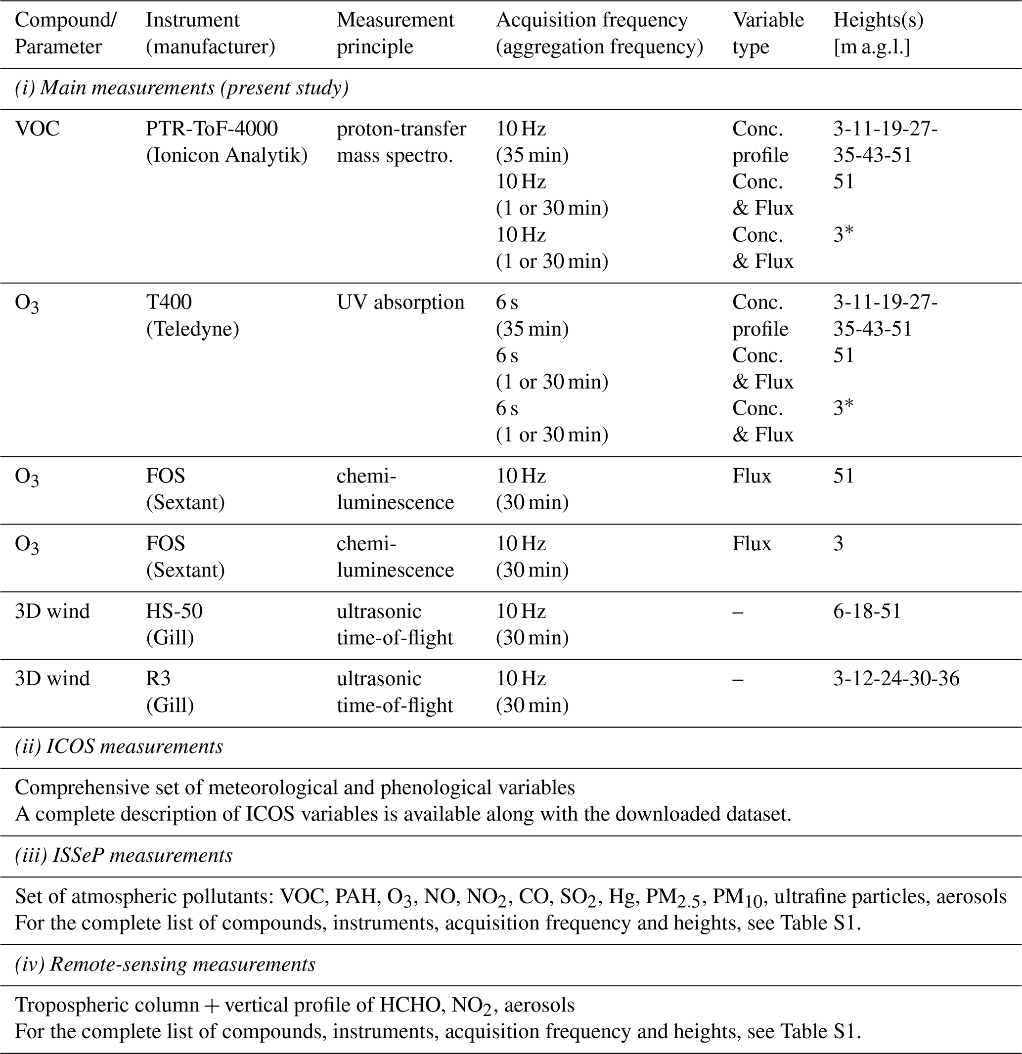
^* Not available in 2022.

In the shelter, ambient air was subsampled towards a PTR-ToF-MS 4000 (Ionicon Analytik GmbH, Innsbruck, Austria) instrument for fast measurements (10 Hz) of VOC mixing ratios. On the same line, air was also subsampled towards a T400 UV Absorption O₃ analyser (Teledyne Technologies Inc, San Diego, CA, USA) for low-frequency measurements (every 6 s) of ozone. Section 2.2.4 provides more information about the pneumatic system inside the shelter.

The T400 instrument was used to deliver calibrated concentrations of ozone, but its measurement frequency was not suitable for flux computation. Therefore, an additional Fast Ozone Analyser (FOS, Sextant Technology Ltd, Wellington, New Zealand) was installed at the top of the tower. Ambient air was sampled close to the sampling point of the VOC/O₃ line and brought to the FOS analyser through a 6.5 m long and 6.4 mm inner-diameter PFA tube with a flow rate of about 3.5 SLM. This line was also heated, thermally insulated, and protected by a PFA raincap and a PTFE particulate filter. The FOS signal was recorded at a frequency of 10 Hz.

2.2.2 TRUNK system

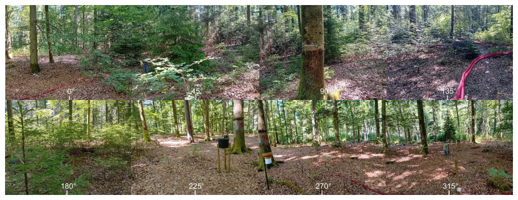
The lowest level of the VOC/O₃ profile (H1, see Sect. 2.2.3) was located on a 3 m high mast installed in 2022 in the European beech sector, approximately 10 m west of the tower. Ambient air was sampled through a 60 m long tube leading to the shelter. In 2023, a second FOS instrument (5 m long and 6.4 mm inner-diameter PFA tube, flowrate of 3.5 SLM) and a 3D R3-50 sonic anemometer (Gill Instrument Ltd, UK) were added to the 3 m mast to establish a system compatible with EC measurements. This configuration, referred to as the TRUNK system, samples air from within the trunk space of the forest, primarily to characterize the VOC and ozone fluxes exchanged by the soil. However, a small part of this space is occupied by young woody vegetation, shrubs, mosses and ferns, as shown in Fig. 3.

Figure 3 Panoramic view (360°) taken from the mast of the TRUNK system in summer 2023.

2.2.3 PROFILE system

The characterization of exchange processes inside the canopy is based on two types of profiles: (i) a VOC and O₃ concentration profile and (ii) a turbulence profile measured using 3D sonic anemometers. The two 60 m long lines installed for the TRUNK and TOP systems were supplemented by five additional tubes of the same length, material and diameter, resulting in a concentration profile with seven evenly distributed sampling points. The measurement heights for levels H7–H1 are given in Table 1 and Fig. 2. All of these lines were made of PFA, heated, and connected to a manifold inside the shelter. The TOP and TRUNK sonic anemometers were supplemented by an additional HS-50 and R3-50 sonic anemometers, respectively mounted on 3 and 2 m long aluminium arms attached to the tower. These sonic anemometers were rotated over the 3-year measurement period to characterize turbulence at as many heights as possible. The corresponding heights are listed in Table 1.

2.2.4 Pneumatical setup

In the shelter, a manifold system made of seven three-way PFA solenoid valves was used to sequentially sample ambient air from levels H7 to H1. During TOP (H7) and TRUNK (H1) system measurements, air was sampled for at least 30 min to apply the EC method. In PROFILE mode, air was sequentially sampled from levels H6 to H1, for respective periods of 5 min. To obtain a complete concentration profile, the last 5 min of a preceding TOP mode were included in the PROFILE cycle.

Downstream of the manifold, air was subsampled towards the PTR-ToF-MS and T400 instruments. Due to the pressure drop along the 60 m sampling line, the inlet pressure of the T400 becomes too low for proper operation. To compensate for this, a PTFE-coated membrane pump (KNF N86KT.18, KNF Neuberger GmbH, Freiburg, Germany) was installed upstream of the T400 to bring the sampled air to local atmospheric pressure. The PTR-ToF-MS requires regular calibration and background measurements. For background measurements, the ambient air subsampled from the H7 line was sent through a catalytic converter (Parker, type HPZA-3500, Haverhill, MA, USA) to remove VOC before being analysed. For calibration, a user-defined flow rate of a VOC standard (Apel-Riemer Environmental Inc., FL, USA) was mixed with zero-VOC air from the background line. More details on VOC quantification are given in Sect. 2.3.2. A total flow of about 10 SLM was pumped through the selected sampling line by a membrane pump (MD12C NT, Vacuubrand, Germany) and manually controlled by a needle valve. A buffer volume was added between the needle valve and the flow meter to dampen the flow and pressure variations caused by the pump. The non-selected sampling lines were continuously flushed with ambient air to allow for fast switching between lines.

2.2.5 Data coverage

During the 3 years of measurements, the VOC and O₃ analytical instruments were operated as simultaneously as possible, with particular emphasis on the spring, summer, and autumn periods. Figure 4 summarizes the monthly percentages of half-hour intervals that were successfully measured by each system.

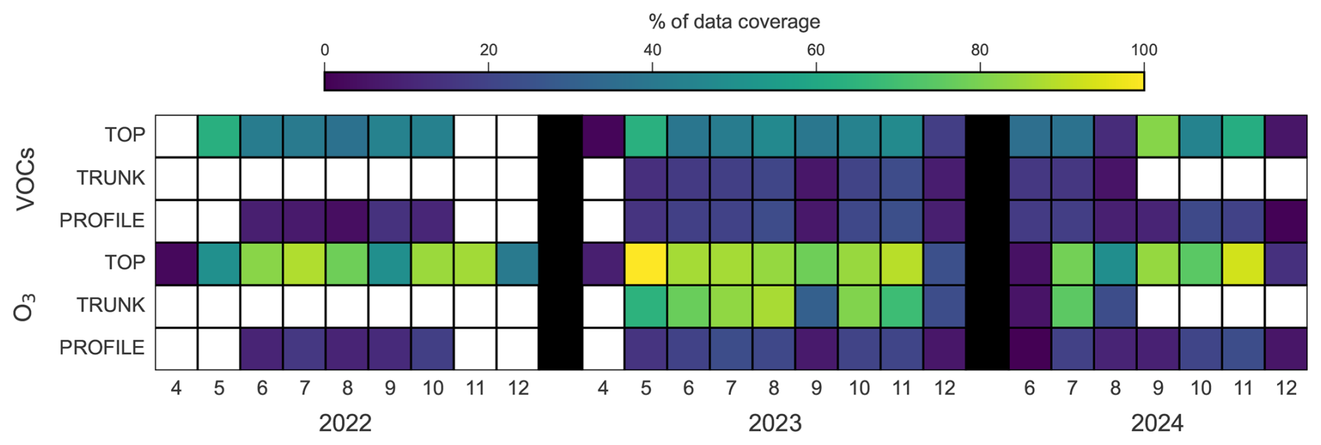
Figure 4 Percentage of half-hours covered per month and per year for measurements shared between the TOP, TRUNK and PROFILE systems.

In 2022, the PTR-ToF-MS and the T400 instruments sequentially measured 30 min periods at the TOP level and in PROFILE mode. On average, TOP measurements were performed 3.5 times more frequently than PROFILE measurements. Background VOC measurements were systematically performed for 30 min every 4 h, and single-point VOC calibrations were performed every 3 to 4 d. These procedures limited data coverage for other measurement systems.

In 2023 and 2024, TRUNK measurements were added. In this updated sequence, TOP measurements occurred on average 2.5 times more frequently than PROFILE or TRUNK measurements.

Overall, ozone flux measurements at the TOP and TRUNK levels were more frequent than those for VOCs, since the two FOS analysers operated continuously, while the PTR-ToF-MS had to alternate between levels. This will be discussed further in Sect. 2.4.2.

2.3 VOC measurements

2.3.1 PTR-ToF-MS settings

The PTR-ToF-MS instrument was operated in the H₃O⁺ mode. Air was subsampled by the instrument through a 1.2 m long silcosteel capillary (1 mm inner diameter). The drift tube reactor was operated at a pressure of 3.3 hPa and a reduced electric field ($E/N$) of 135 Td (1 Townsend = 10⁻²¹ V m²). Both the inlet line and the drift tube reactor were kept at 353 K. The inner part of the drift tube has an EVR (Extended Volatility Range, Piel et al., 2021) coating to minimize losses of sticky compounds to the surfaces of the reactor. A hexapole ion guide is used to efficiently transport ions from the drift tube to the mass analyser section.

The Time-of-Flight mass spectrometer was operated at an extraction time and frequency of 2 µs and 40 kHz, respectively, allowing for a mass-to-charge ($m/z$) range of 7–392. A small flow of diiodobenzene, provided by a built-in permeation device (PerMaSCal, Ionicon Analytik GmbH, Innsbruck, Austria) was constantly added to the drift tube for frequent internal mass scale calibration based upon the position of protonated diiodobenzene (at $m/z$ 330.848), its fragment (at $m/z$ 203.943), and H${}_{\mathrm{3}}^{\mathrm{18}}$O⁺ (at $m/z$ 21.022) on the detector. Time-of-flight mass spectra were integrated over 100 ms to allow for EC flux calculations. A maximal mass resolution ($m/\mathrm{\Delta }m$) of 4200 was obtained for the high mass range. At $m/z$ 59.049 (protonated acetone) and $m/z$ 137.132 (protonated monoterpenes), the mass resolution was about 3400 and 3800, respectively. The peak area related to primary ion signals ranged from 8766–25554 ($m/z$ 21.022 related to H₃O⁺) to 11–619 ($m/z$ 38.033; H₃O⁺(H₂O)) counts per second (cps) over the 3 years of measurements. By considering the relative transmission of the instrument at $m/z$ 21.022 and 38.33 (respectively 9 %–15 % and 29 %–43 % relative to the transmission at $m/z$ 180.937), together with the relative abundance of the H${}_{\mathrm{3}}^{\mathrm{18}}$O⁺ and H${}_{\mathrm{5}}^{\mathrm{17}}$O¹⁶O⁺ + DH${}_{\mathrm{4}}^{\mathrm{16}}$O${}_{\mathrm{2}}^{+}$ isotopes (respectively 488 and 669), this results in a transmission-corrected source ion count rate of 40×10⁶–110×10⁶ cps.

2.3.2 Signal processing and quantification

Peak identification and integration of recorded spectra were performed on a near-daily basis with the Ionicon Data Analyzer software (IDA Müller et al., 2013; 2022, v 1.0.0.2; 2023, v 2.0.1.2; 2024, v 2.2.1.1). Subsequent data processing was performed in a python-based framework referred to as the Peak Area Processing software (PAP) which was used for non-targeted peak selection, instrument characterization, and quantification of mixing ratios with related uncertainties at both 10 Hz and 1 min time resolution. The PAP software is publicly available (https://github.com/bverreyk/PeakAreaProcessing, last access: 13 January 2026, Verreyken et al., 2025a) and a general overview of its main processing steps is given below. An extended version of the discussion on how VOCs were quantified and details on the configuration of the PAP software and instrument operations can be found in Sect. S2.

Mass selection

The mass scale was calibrated in the IDA software every 60 s and peak-shapes were considered stable over the course of 1 h. Independent peak identification was performed for each IDA analysis with up to 8 $m/z$ values identified per peak system (collection of isobaric peaks with the same nominal mass). A peak system was only considered for analysis if its maximum ion signal intensity exceeded 0.1 cps. To obtain a list of non-targeted $m/z$ ratios, Density-Based Spatial Clustering of Applications with Noise (Ester et al., 1996), or DBSCAN, was employed to identify mass-to-charge ratios where peaks were regularly observed. An automated selection of ion $m/z$ values has been performed based on (i) the width of the DBSCAN intervals centred around the mass (stability of peak identification by IDA), (ii) the fraction of data above the limit of quantification (significance of concentrations), and (iii) the $m/z$ localization (interpretability of the data). Afterwards, a manual selection to discard $m/z$ values related to isotopes or hydrated ion species was done. Compound attribution was performed by making use of PTR-MS databases (Pagonis et al., 2019; Yáñez-Serrano et al., 2021) and measurements reported at ecosystem sites (Kim et al., 2010; Hellén et al., 2018; Schallhart et al., 2018; Pfannerstill et al., 2021) to identify the compounds most likely to contribute to the observed signal.

Instrument characterization

Calibrations were performed every 3–4 d to characterize the instrument transmission and calculate calibration factors for compounds included in the calibration bottle (Table S2). Instrument transmission (relative to the one at $m/z$ 21.022) was calculated using a subset of compounds (associated to $m/z$ 33.033, 42.034, 45.033, 59.049, 79.054, 93.070, 107.086, and 180.937) included in the calibration bottle (Fig. S2). The transmission curve between $m/z$ 21.022 and 180.937 was defined through linear interpolation of transmissions obtained during calibrations. At high $m/z$, the transmission curve becomes more stable and we assumed a constant behaviour (${\mathrm{Tr}}_{mz>\mathrm{180.937}}\equiv {\mathrm{Tr}}_{\mathrm{180.937}}$).

Mixing ratio calculation

The mixing ratio of compounds was calculated using either the kinetic or the calibration approach, similar to the discussion in the ACTRIS measurement guidelines for VOC analysis with PTR-MS instruments (Dusanter et al., 2025). In both cases, integrated peak areas (cps) obtained from IDA were corrected for ion transmission, and normalized with respect to a source ion peak area of 10⁶ cps to account for variations in the source ion production. VOC volume mixing ratios (VMR) were calculated by dividing the background-subtracted transmission-corrected normalized peak areas (tc-ncps) by the compound-dependent sensitivities (tc-ncps ppbv⁻¹). For compounds present in the calibration standard, sensitivities were calculated at every calibration. At $m/z$ values not related to compounds available in the standard, sensitivities were derived from calculated H₃O⁺/VOC reaction rate constants and product ion distributions, as well as drift tube reactor conditions, as explained in more detail in Sect. S2.1.3.

Uncertainty quantification

The expanded or combined uncertainty (with a coverage factor of 2) of the calculated VOC mixing ratios combines both the precision of the peak areas and systematic errors (accuracy) associated with instrument calibration or sensitivity calculations:

$$\begin{array}{}\text{(1)}& \mathrm{expanded}\mathrm{uncertainty}=\mathrm{2}\cdot \sqrt{{\mathrm{precision}}^{\mathrm{2}}+{\mathrm{accuracy}}^{\mathrm{2}}}\end{array}$$

The precision of the peak areas can be determined from Poisson statistics and approximated by the square root of the integrated counts over the measurement interval. However, peak areas obtained with IDA are inherently baseline-subtracted (Müller et al., 2013) and can be negative for small peaks, hereby invalidating the above-mentioned approach. This issue occurs especially during zero measurements and is more prevalent when considering data acquired at high sampling frequency, where statistical uncertainties are inherently higher. For 1 min averaged data, the precision was therefore approximated by the precision of the mean 100 ms peak area over the variability interval, assuming a normal distribution.

The systematic uncertainty (accuracy) of the volume mixing ratios for compounds included in the calibration standard was obtained by combining the stated uncertainty on the mixing ratios of those compounds in the standard (∼ 2.5 %) with the uncertainty of the dilution factor (∼ 1.5 %). A conservative systematic uncertainty of ∼ 56 % was used for mixing ratios quantified using the kinetic approach, due to large uncertainties on the calculated H₃O⁺/VOC rate constants (∼ 25 %) and on the product ion distributions (∼ 50 %). This accuracy is close to results by Sekimoto et al. (2017) which showed that measured sensitivities agreed within 20 %–50 % with theoretical sensitivities calculated using molecular mass, elemental composition, and functional group of the analyte.

For the combined uncertainty, Simon et al. (2023) included an additional 5 % uncertainty due to relative humidity effects. However, as the H₃O₊(H₂O) signal was generally less than 3 % that of H₃O⁺ + H₃O⁺(H₂O) (Fig. S4), the impact of relative humidity was assumed to be small and this additional uncertainty is not considered here.

The limit of detection (quantification) for concentrations is defined as three (ten) times the precision of the associated background measurement, of which we only considered the last 5 min to assure equilibrium. The mean and standard deviation of the measurement distribution during these 5 min were used to define the background value and its precision, respectively.

More details on uncertainty characterization are given in Sect. S2.1.4.

2.3.3 Flux computation

Half-hourly VOC fluxes were computed following the general procedure commonly used for eddy covariance flux calculation. This included raw data despiking and gap filling, block averaging, coordinate rotation of wind components, time-lag estimation by maximizing covariance and data shifting, covariance calculation and correction for high-frequency spectral losses (Aubinet et al., 2012).

EC fluxes are commonly filtered to remove data collected under low-turbulence conditions, particularly for CO₂ fluxes, using a friction velocity (u^*) threshold. However, given the different nature of VOC exchange processes compared to CO₂, no u^* filtering was applied in this study. Additional information and justification for this choice are provided in Sect. S3.1.

All flux computations, from raw sonic anemometer data and processed VOC concentrations, were performed using the GEddySoft (“Gembloux Eddy-covariance Software”) software. GEddySoft was initially developed from the open source innFlux software (Striednig et al., 2020), which supports both conventional and disjunct eddy covariance analyses. The original MATLAB^® code was converted to Python, and the software has been continuously expanded with additional data handling and flux processing features. For this study, version 4.0 of GEddySoft was used and is publicly available (https://github.com/BernardHeinesch/GEddySoft, last access: 13 January 2026), along with a test input dataset (https://doi.org/10.18758/IYPN6FNM, Heinesch et al., 2025).

Unless explicitly stated, the same procedure was applied to both the TOP and TRUNK systems. One exception concerns the tilt correction of the sonic anemometers: the double rotation method was used for the TOP system, while the sector-wise planar fit method was applied to the TRUNK system. Below-canopy turbulence was sometimes low, so applying the double rotation method at the half-hourly scale could result in high rotation angle values and erroneous fluxes (notably artificially high absolute fluxes; see Fig. S6, where the effect is most visible for O₃ fluxes). The sector-wise planar fit method, which computes a single set of tilt angles based on long-term time series, was able to solve this issue and was therefore applied to TRUNK fluxes (with tilt angles determined for 2023 and applied to both 2023 and 2024). Details about both methods are given in Wilczak et al. (2001). The structure at the back of the sonic anemometer used for the TOP system (HS-50) can act as an obstacle to airflow. Consequently, fluxes coming from a ±10° wind sector around the sonic anemometer arm were discarded, following the ICOS protocol (Sabbatini et al., 2018). No filtering was applied to TRUNK fluxes, which were measured with an omnidirectional sonic anemometer.

The main steps of flux computation described above were also applied to ozone fluxes. However, considering the differences in the measurement setups, several methodological aspects diverged between the two flux calculations. These aspects are detailed in the present Section for VOCs and in Sect. 2.4.1 for ozone.

Lag time determination

In EC measurements, the lag time represents the time delay between instantaneous measurements of the vertical wind component w and the tracer concentration c, arising, among other factors, from differences in electronic signal processing, spatial separation between wind and scalar sensors, and air transport through sampling lines (Aubinet et al., 2012). When w and c are recorded on separate data logging systems, it is therefore good practice to regularly synchronise their internal clocks in order to minimise clock drift, which would otherwise introduce an additional temporal offset between the two time series.

In the present set-up, w and c were recorded on two distinct laptops, which were frequently synchronised using a GPS time reference (MR-350, GlobalSat WorldCom Corporation, Taipei Hsien, Taiwan). However, while the computers themselves remained synchronised, the internal data acquisition system (DAQ) of the PTR-ToF-MS relied on a separate internal time axis, which exhibited a non-linear time drift, the origin of which could not be fully identified. As a consequence, the timestamps assigned to the mass spectra by the DAQ progressively became de-synchronised from the sonic anemometer time series. To overcome this issue, the evolution of this drift was monitored during each field campaign and used to correct for the DAQ-related time drift during post-processing. In addition, the DAQ was regularly restarted during the campaigns in order to minimise the accumulation of this time drift and reset it to zero.

After correction for the DAQ-related time drift, the lag time between w^′ and c^′ was determined by maximizing their covariance within a physically plausible window (11–15 s) for each flux window and each $m/z$. If the maximum covariance occurred at the edge of the window, a fixed lag of 13 s was assigned. This default value corresponds to both the centre of the window and the median lag time observed for monoterpenes (VOC with the highest signal-to-noise ratio, SNR) across the entire measurement campaign. It is also consistent with expectations based on tube dimensions and flow rates (first-order estimate of the residence time, ∼ 10 s).

To refine lag estimation and reduce spurious detections under low SNR conditions, the covariance function was smoothed using a 15-sample (1.5 s) moving average prior to the search. This approach, as recommended by Taipale et al. (2010) and Langford et al. (2015), effectively mitigates “mirroring” effects associated with low fluxes while preserving sensitivity to time-varying lags.

The stability of lag times was assessed visually across all campaigns and for all $m/z$ values. Under high SNR conditions, lag times were found to be highly stable, with the exception of two ions species: 33.033 (protonated methanol) and 47.049 (protonated ethanol) (as well as H₃O⁺ and its hydrates, which were excluded from the analysis). For these two $m/z$, a small but systematic dependence on air relative humidity (RH) was observed. When RH exceeded 95 %, the lag time tended to increase in absolute value, shifting from −13 up to −20 s (data not shown). Consequently, the centre of the lag-search window was parametrized as a function of RH for these two ions.

Correction for flux high-frequency losses

An experimental co-spectral approach was adopted to correct for high-frequency attenuation (Aubinet et al., 1999; Wintjen et al., 2020), and was applied in three steps. First, a transfer function was derived by dividing the normalized mean co-spectrum of wc (attenuated) by that of wT (considered ideal), and was then fitted using a Lorentzian function to obtain a single cut-off frequency. Second, to derive a flux correction factor at the half-hour scale, the area under the wT co-spectrum (representing the non-attenuated flux) was divided by the area under the same co-spectrum multiplied by the transfer function (representing the attenuated flux). Third, these correction factors, obtained for a limited number of half-hours after drastic data filtering (see Sect. S3.3), were sorted and averaged into five wind speed classes for unstable and stable atmospheric conditions separately. These two lookup tables were then used to assign a correction factor for each individual half-hour, depending on its wind speed and atmospheric stability. The procedure was applied to monoterpenes to benefit from their high SNRs. Since the correction characterizes the experimental setup in combination with the flow characteristics, without any expected compound-specific aspects, it was then applied to all other compounds.

The choice of a co-spectral, rather than spectral, approach was motivated by its capacity to empirically integrate all causes of signal attenuation – tube damping, instrumental response, and sensor separation – without relying on a theoretical transfer function for sensor separation. Furthermore, our method does not require a reference co-spectrum, whose formulation and ability to represent real conditions at the site are often subject to discussion. It should be noted that, following the recommendations of Peltola et al. (2021), the square root of the transfer function was used rather than the transfer function itself to derive both the cut-off frequency (step one) and the correction factor (step two), in order to correctly account for the phase shift introduced by our lag-time determination method.

For the TRUNK system, step one could not be applied due to generally low fluxes and associated low SNRs across all compounds. However, given that the cut-off frequency reflects the setup alone and that the TRUNK and TOP configurations were identical, the cut-off frequency derived from the TOP system was applied. Steps two and three were executed independently for the TRUNK level, as atmospheric turbulence is location-specific.

This procedure led to correction factors ranging from 1.10 to 1.26 for the TOP system, and from 1.10 to 1.40 for the TRUNK one. More details are provided in Sect. S3.3.

Flux quality control

Flux quality was assessed at two levels. First, the high-frequency inputs used for flux computation – VOC mixing ratios and sonic anemometer data – were (in)validated based on statistical tests developed by Vitale et al. (2020). These tests have the advantage, compared to the more traditional tests of Vickers and Mahrt (1997), of being completely automatable, not requiring user choices on, for example, threshold values. Adapted from the open-source RFlux toolbox (https://github.com/icos-etc/RFlux, last access: 3 July 2025), they were integrated in our GEddySoft processing pipeline. The combination of the tests present in RFlux and described in Vitale et al. (2020) (HF₅, HF₁, HD₅, KID) led to the creation of an instrumental flag, hereafter named flag_instr. Only a few half-hour periods were flagged for instrumental issues (Fig. S12), with a maximum of 12 % of fluxes flagged for $m/z$ 80.058 in the TOP system.

Other instrumental tests available in the RFlux toolbox – including AL1, DIP, and DDI – although implemented in the ICOS standard processing pipeline, were not applied here. These tests tended to flag excessively long periods, including VOC fluxes with low SNR, as well as those displaying clear and reasonable diurnal dynamics. Furthermore, they have not yet been described in peer-reviewed literature and have never been validated for compounds with inherently lower SNR such as VOCs. For these reasons, they were considered unsuitable for our dataset and were excluded from the present analysis.

Second, a quality flag was assigned to the computed fluxes based on steady-state (stationarity) and integral turbulence characteristic tests, following the methodology developed by Mauder and Foken (2004). This flag, named flag_MF (for Mauder and Foken), can take three values: 0 indicates high-quality fluxes; 1 corresponds to fluxes suitable for general analysis; and 2 denotes poor-quality fluxes. For stationarity, we preferred the test proposed by Mahrt (1998) over that of Foken and Wichura (1996), as it proved more effective at flagging anthropogenic influences (see Sect. 2.3.4). Fluxes flagged at level 2 were discarded for the remainder of this study. The percentage of half-hours discarded according to flag_MF reached up to 20 % for the TOP system and 33 % for the TRUNK system, in both cases for $m/z$ 137.132. This filtering is primarily due to the influence of anthropogenic sources (see Sect. 2.3.4), an effect further described in Sect. S3.4.

A combined flag (flag_tot) was created by integrating flag_instr and flag_MF, as well as an additional flag (flag_plume) designed to filter out periods affected by anthropogenic emissions (see Sect. 2.3.4). Only fluxes passing all three flag criteria were assigned a value of 0 for flag_tot and retained for further analysis in this study.

Correction for density fluctuation

VOC fluxes can be biased by fluctuations in temperature and water vapour, which affect air density. These effects can be accounted for using the Webb–Pearman–Leuning (WPL) corrections (Webb et al., 1980). In our setup, temperature fluctuations were considered attenuated due to the length of the sampling lines, which largely exceeded the 3.20 m minimum recommended by Rannik et al. (1997). Moreover, during flux measurements using a PTR-ToF-MS, Loubet et al. (2022) reported that corrections for water vapour fluctuations were very small (less than 2 % for 75 % of the time). For these reasons, WPL corrections were not applied to VOC fluxes in this study.

Flux storage

To obtain the net exchange of VOCs, a storage term should be added to the turbulent flux. The storage flux represents the temporal variation of the mixing ratio of the compound below the EC measurement height, and is expected to be non-negligible for tall towers and under low turbulence conditions, such as at night. The storage term was calculated following the procedure described by Montagnani et al. (2018):

$$\begin{array}{}\text{(2)}& S_i=\sum _{j=\mathrm{1}}^N{\mathit{\rho }}_{{\mathrm{d}}_j}{\left({\displaystyle \frac{\mathrm{\Delta }{c}_i}{\mathrm{\Delta }t}}\right)}_j\mathrm{\Delta }{z}_j\end{array}$$

where S_i is the storage flux for tracer i (nmol m⁻² s⁻¹), ${\mathit{\rho }}_{{\mathrm{d}}_j}$ is the dry air density of layer j, ${\left(\frac{\mathrm{\Delta }{c}_i}{\mathrm{\Delta }t}\right)}_j$ is the temporal variation of mixing ratio for tracer i (nmol mol⁻¹) at height j over a time period Δt (s), and Δz_j is the thickness of layer j (m). Temporal changes in mixing ratios were derived from concentration profiles measured every 2 to 2.5 h.

The resulting storage fluxes exhibited erratic temporal dynamics and, for many VOCs, their magnitudes often exceeded those of the turbulent flux. We consider that calculating temporal variations in concentrations over 2 to 2.5 h intervals is unlikely to accurately capture true storage processes within the canopy, particularly for reactive compounds with short atmospheric lifetimes. This limitation likely results in unreliable storage flux estimates. To avoid degrading the overall data quality, storage fluxes were therefore not included in the net flux calculation.

2.3.4 Filtering of anthropogenic sources

Over the 3 years of measurements, we occasionally observed abnormally high VOC mixing ratios under winds from the 230–270° sector. This phenomenon had already been reported for monoterpenes and methanol during earlier campaigns in 2009 and 2010 (Laffineur et al., 2011, 2012), and was attributed to a wood panel factory located 3 km south-west of the tower.

In the present study, this anthropogenic influence was mostly observed at night, yet occurred irregularly and did not affect all VOCs uniformly, with many of the detected ions not being impacted at all. The most affected ions included protonated monoterpenes (e.g. $m/z$ 137.132), as well as fragments and isotopes, sesquiterpenes, and potential derivatives such as $m/z$ 135.117 (likely p-cymene). A few low molecular weight oxygenated compounds such as methanol and acetic acid were also affected, though to a lesser extent. During plume events, the affected VOCs exhibited elevated mixing ratios and mixing ratio variances, and occasionally large negative fluxes (i.e. apparent deposition), which are not expected for compounds like monoterpenes.

To identify such episodes, Laffineur et al. (2011) proposed an upper threshold on the 30 min variance of monoterpene mixing ratios in the 230–270° wind sector, assuming that incomplete mixing between anthropogenic and biogenic sources led to higher variability in mixing ratios. However, extending this method would require manually identifying all impacted ions and setting compound-specific thresholds, which is subjective and impractical.

To address this limitation, we developed an automatic flagging procedure. For each VOC, we computed q₉₉, the 99th percentile of its 30 min mixing ratio variance calculated across all wind directions except 180–300°, which is subject to sawmill influence. Then, any half-hour within the 180–300° sector with a variance exceeding q₉₉ was flagged as potentially affected (Fig. S11). This approach successfully identified affected VOCs (7 % of half-hours flagged for monoterpenes or methanol, see Fig. S12) while leaving unaffected compounds mostly untouched (e.g. only 0.3 % flagged for isoprene). Although many spoiled half-hours had already been identified by the stationarity test (flag_MF), this new flag_plume completed the identification of such events.

Two mechanisms may account for the influence of the sawmill on local fluxes despite their relatively long distance from the tower (3 km). First, although the factory typically falls within an area with a low relative contribution to the measured flux compared with the surrounding forest, its clear influence observed in the fluxes suggests that the sawmill would constitute a strong VOC source. This influence is most evident at night, when more stable atmospheric conditions enlarge the flux footprint, thereby increasing the relative weight of the factory on the observed fluxes. A second explanation is that even when the factory lies in a footprint region with very low contribution, VOC-rich air masses emitted by the factory may still be advected toward the tower. In such cases, the resulting high local concentrations can generate apparent downward fluxes, despite the source being located outside the main footprint area.

While some fluxes exhibited a well-defined lag time during plume events – suggesting real turbulent deposition, as also observed by Bamberger et al. (2011) – these episodes showed erratic dynamics and no consistent relationship with environmental drivers. Therefore, to focus the analysis on biogenic VOC exchange, we excluded flagged fluxes from further processing. Similarly, concentrations flagged by flag_plume were not considered in the rest of this study.

2.3.5 Identification of significant exchanges

Among the $m/z$ retained by the DBSCAN algorithm, not all ions exhibited significant fluxes. To determine whether a compound is significantly exchanged, it is common practice to compare half-hourly fluxes with their corresponding flux limit of detection (LOD_f). In this study, LOD_f was estimated at the 99 % confidence level as three times the random flux error, calculated in GEddySoft following the method described in Finkelstein and Sims (2001).

Extrapolating such comparisons from the half-hourly scale to longer periods, in order to assess whether a compound is consistently exchanged, is not straightforward. Loubet et al. (2022) addressed this by comparing the mean flux of VOCs with an averaged LOD_f, itself calculated as the square root of the sum of squared individual LOD_f values, divided by the number of records (Langford et al., 2015). While this approach allows a simple comparison over an entire campaign, it may fail to detect compounds significantly exchanged only during short periods.

To overcome this limitation, we developed a novel three-step methodology, applied individually to all $m/z$ values. First, each half-hour period was flagged as significant if the absolute flux exceeded its LOD_f. Second, a day was considered significant if at least 25 % of the daytime half-hourly periods (defined as 08:00–20:00 LT) were significant. Finally, we considered the number of consecutive significant days. Given that the mechanisms responsible for VOC emission or deposition are unlikely to occur on a single day, we selected $m/z$ values for which at least 3 consecutive days of significant exchange were observed during the measurement period.

2.4 Ozone measurements

2.4.1 Raw ozone fluxes

Ozone flux measurements were performed with a fast ozone analyser (FOS). In the instrument, O₃ molecules present in ambient air react with a coumarin disc (solid or dry phase), thereby producing a light signal (chemiluminescence reaction) recorded in units of Volts (V) at a high frequency (10 Hz). Coumarin discs were produced from silica plates impregnated with a solution of coumarin, methanol and ethylene glycol. Since the efficiency of the chemiluminescence reaction decreases over time, coumarin discs were replaced on average once a week during the 2022 and 2023 campaigns. In 2024, disc replacements were less frequent considering the important workload (up to 36 d between disc replacements).

Raw ozone fluxes were computed using the EddyPro^® software, applying the same processing steps as described in Sect. 2.3.3. As for VOCs, no u^* filtering was applied. Given the differences in the measurement setups, certain aspects of the flux computation differ and are detailed below.

Lag time determination

As for VOCs, the physical lag time between w^′ and c^′ was determined by maximizing the covariance function within a predefined lag window. When no clear extremum was found within this window, a nominal lag value was applied. Due to the higher SNR of O₃ fluxes compared to many VOCs, no smoothing of the covariance function was necessary. Across the different measurement campaigns, the median lag time was close for the O₃ TOP and TRUNK systems, with values of 2.2 and 2.0 s, respectively.

Correction for flux high-frequency losses

The three-step experimental co-spectral approach applied to VOCs was also used for ozone. The only difference is that, due to more pronounced ozone fluxes measured at the TRUNK level compared to VOCs, it was possible to determine a cut-off frequency for the TRUNK system.

Correction factors ranged from 1.12 to 1.37 for the TOP system, and from 1.03 to 1.28 for the TRUNK one. Further details are provided in Sect. S3.3.

Flux quality control

An instrumental flag was generated by combining the individual tests developed by Vickers and Mahrt (1997) and implemented in EddyPro^®. The attack angle and non-steady wind tests were excluded, as they tended to over-flag data that did not appear problematic upon visual inspection. Very few half-hour periods (<1 %) were affected by instrumental issues (Fig. S12).

EddyPro^® also computes a flux quality flag similar to the previously described flag_MF, based on the stationarity test of Foken and Wichura (1996). Over the 3-year period, 9 % of the fluxes were flagged as level 2 (poor quality) for the TOP system, and 17 % for the TRUNK system (Fig. S12).

No influence from the wood factory was detected in the ozone data; therefore, no flag_plume was applied. Data flagged by flag_tot were excluded from further analysis in this study.

Correction for density fluctuation

From the original WPL equation (Webb et al., 1980), we neglected temperature fluctuations – assumed to be attenuated through the sampling tubing, as for VOCs – and only assessed the impact of water vapour fluctuations. The latter resulted in a correction of less than 1 % of the raw fluxes on average. This value is much lower than the one reported in Gerosa et al. (2022a) – where temperature-related corrections could not be neglected considering the large-diameter tubing – and also well below our flux random uncertainty estimated according to Finkelstein and Sims (2001). For these reasons, no WPL correction was applied.

Flux storage

The ozone storage was computed with Eq. (2). For TOP storage, 7 layers were considered (H1 to H7, see Fig. 2). Profile measurements were taken every 2 or 2.5 h, so half-hourly storage values were linearly interpolated between adjacent measurements. Since profiles were not continuously scanned throughout the measurement campaigns, a gap-filling approach was required. For TOP storage, we used the storage computed from TOP mixing ratio (which was available at least once every three half-hours) as a proxy for the actual storage term. In combination with other predictors (friction velocity u^*, air temperature, incoming PPFD at the top of the canopy, hour of the day, and month number), we trained a Random Forest regression model to estimate and gap-fill storage fluxes derived from the concentration profile. This procedure represents an improvement over the methodology used by Aubinet et al. (2018), who employed look-up tables to gap-fill missing storage data.

No model was required to gap-fill TRUNK storage fluxes. Since only one layer was considered, the storage flux was computed directly when the T400 was in PROFILE mode (using level H1) or TRUNK mode. The missing half-hour values were linearly interpolated between adjacent data points, provided that gaps were shorter than 3 h.

Unlike for VOCs, ozone storage showed a consistent diel pattern (Fig. S14, similar to that observed by Finco et al., 2018). We therefore decided to add the storage flux to the calibrated turbulent flux (calibration described in Sect. 2.4.2) to obtain the net ozone flux.

2.4.2 Ozone flux calibration

Since the FOS analyser provides only voltages (V) proportional to the ozone concentrations, the raw fluxes were calibrated using a T400 UV absorption analyser, which delivers absolute and stable O₃ mixing ratios in ppbv (nmol mol⁻¹). The T400 instrument was calibrated annually before each measurement campaign, and automatic zero and span checks were performed nightly to monitor potential drifts.

As noted in Muller et al. (2010) and Zhu et al. (2015), calibration procedures for FOS-based ozone fluxes are rarely detailed, despite their significant impact on data quality. The FOS analyser's sensitivity decreases over time due to the consumption of coumarin molecules in the chemiluminescence reaction with ozone. This sensitivity loss is therefore non-linear (Güsten and Heinrich, 1996), varies from one disc to another, and may include an offset between fast and slow signals.

Muller et al. (2010) tested three post-processing calibration methods (see Table 2) by comparing fast and slow ozone signals (1) at the half-hourly scale without considering an offset (Ratio Method, RM), (2) at the half-hourly scale with an offset determined for each coumarin disc (Ratio Offset Method, ROM) and (3) over the lifetime of a coumarin disc using a single regression (Disc Calibration Method, DCM). The RM captures changes in FOS sensitivity more effectively than the DCM, which assumes a stable response throughout the disc lifetime. The ROM represents a compromize; although it applies a half-hourly ratio, the offset remains fixed over the disc's life and may not follow short-term sensitivity shifts.

Table 2 Comparison of O₃ flux calibration methods.

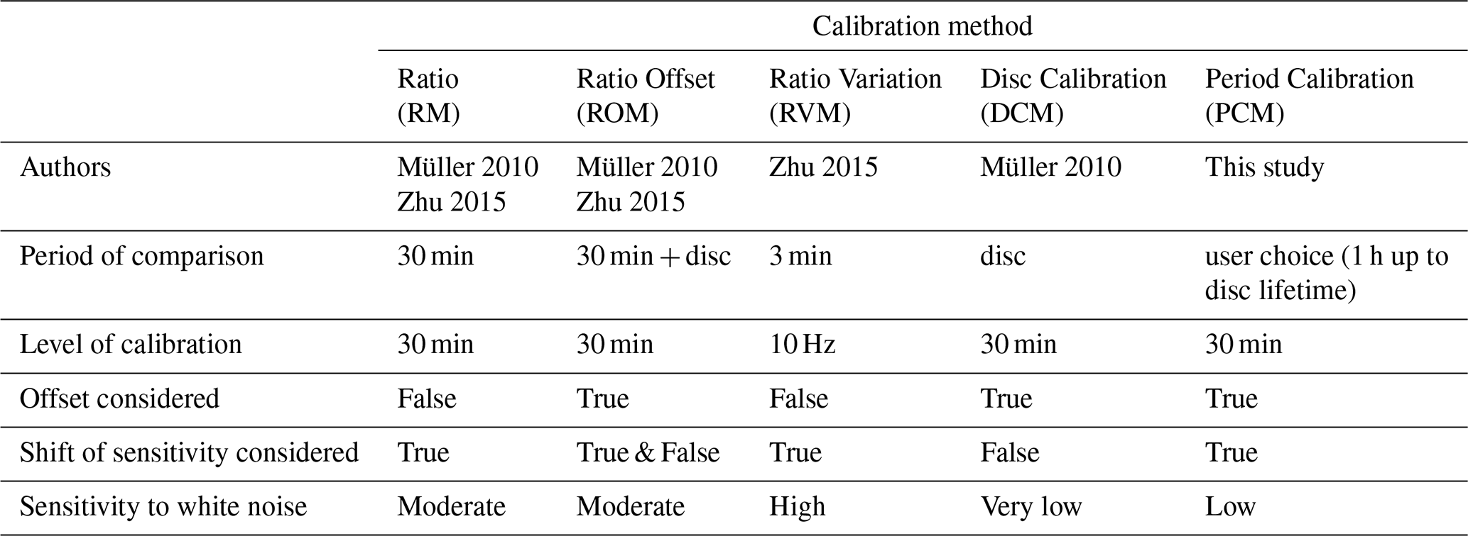
Zhu et al. (2015) later introduced the Regression Variance Method (RVM), which identifies an optimal averaging window between the FOS and T400 signals using Allan-Werle variance analysis. A 3 min period was found to best track sensitivity changes, but it is also more susceptible to white noise than RM and ROM (30 min windows), and especially DCM (multi-day windows). Both RM and RVM assume zero offset between fast and slow signals – an assumption invalidated by observations from Muller et al. (2010) and Zhu et al. (2015).

An important practical constraint in our study was the limited temporal overlap between fast and slow ozone measurements. The T400 analyser alternated between TOP, TRUNK, and PROFILE modes, preventing continuous half-hourly reference data at any one level. Therefore, we developed a new approach: the Period Calibration Method (PCM). Inspired by DCM, PCM accounts for potential offsets and reduces sensitivity to high-frequency noise. However, unlike DCM, it identifies optimal sub-periods during which the FOS sensitivity remained consistent, allowing more accurate tracking of temporal variability in analyser performance.

With the PCM (Period Calibration Method), calibrated fluxes were computed as:

$$\begin{array}{}\text{(3)}& F_{\mathrm{cal}}={\displaystyle \frac{{\mathit{\beta }}_{\mathrm{1}}{F}_{\mathrm{raw}}}{v_{\mathrm{mol}}}}\end{array}$$

where F_cal is the calibrated flux (nmol m⁻² s⁻¹), F_raw is the raw flux obtained from FOS measurements (V m s⁻¹), β₁ is the slope of the regression curve established between the T400 and the FOS measurements (nmol mol⁻¹ V⁻¹), and v_mol is the air molar volume (m³ mol⁻¹). Note that while regressions between the T400 and FOS measurements were established with an intercept, this constant term does not intervene in Eq. (3) because it does not correlate with w^′.

The overall uncertainty associated with the calibrated flux was estimated from Eq. (3):

$$\begin{array}{}\text{(4)}& {\mathit{\epsilon }}_{\mathrm{F},\mathrm{cal}}={\displaystyle \frac{\sqrt{{\left({\mathit{\beta }}_{\mathrm{1}}\cdot {\mathit{\epsilon }}_{\mathrm{F},\mathrm{raw}}\right)}^{\mathrm{2}}+{\left(F_{\mathrm{raw}}\cdot {\mathit{\epsilon }}_{{\mathit{\beta }}_{\mathrm{1}}}\right)}^{\mathrm{2}}}}{v_{\mathrm{mol}}}}\end{array}$$

where ε_F,cal is the calibrated flux uncertainty (nmol m⁻² s⁻¹), ε_F,raw is the raw flux random error as estimated by Finkelstein and Sims (2001) (V m s⁻¹), and ${\mathit{\epsilon }}_{{\mathit{\beta }}_{\mathrm{1}}}$ is the standard error of the slope estimate (nmol mol⁻¹ V⁻¹). The first term under the square root represents the random flux error and the second term represents the calibration error. On average, the calibration error contributed less than 3 % of the total uncertainty. This is in accordance with the observations made by Horváth et al. (2017).

The procedure to establish the regressions between FOS and T400 data comprised four steps:

1. Data validation: FOS and T400 measurements were automatically validated or invalidated based on instrumental parameters such as pressure, flow rate, temperature, and UV lamp status (for the T400). Measurements from the T400 were discarded during the first 3 min following a mode switch (e.g., PROFILE or TRUNK to TOP, PROFILE to TRUNK) due to sensitivity to pressure variations. This delay allowed for pressure stabilization.

2. Data averaging: the FOS signal was averaged to match the T400's resolution at a 6 s timestamp. Unlike the 15 min averaging used by Muller et al. (2010), this finer resolution captured more variability and increased the number of data points for regression. Both T400 and FOS time series were visually inspected to ensure data quality.

3. Data shifting: a time lag was observed between the two 6 s time series, attributed to the difference in tubing lengths (approximately 6 m for the FOS versus 60 m for the T400). To enhance regression quality, the FOS data was shifted by a time lag determined for each regression using covariance maximization. If a clear covariance maximum was not observed, a nominal time lag estimated for the entire measurement campaign was applied.

4. Regression optimization: linear regressions were established using least-squares fits. Equation (3) was applied only when a satisfactory correlation (R²>0.5) between relative (FOS) and absolute (T400) O₃ concentrations was achieved, as in Muller et al. (2010). Selecting the optimal regression period was a trade-off between maximizing the number of half-hour intervals meeting the R² criterion and minimizing calibration-associated uncertainty (Eq. 4). Initially, increasing the regression period (from 1 up to 24 h) enhanced the R² values and reduced slope errors, as the larger dataset countered random fluctuations (white noise). However, beyond a certain period, shifts in the T400-FOS relationship over time reduced R², while slope errors plateaued or increased. To balance these behaviours, different regression windows were tested, and for each year and system, an optimal period was selected (Sect. S3.5). Final regression slopes (β₁) and their associated uncertainty were then used to calibrate raw fluxes and compute the associated uncertainties.

2.5 Ancillary measurements

2.5.1 Other trace gas and particle measurements

Besides the high temporal resolution VOC and O₃ concentration and flux measurements, which are the main focus of this paper, numerous other in situ – both online and offline – measurements of short-lived climate forcers were conducted at the nearby ISSeP air quality station. In addition, remote sensing measurements of NO₂, HCHO, and aerosols were carried out from the top of the tower. For completeness, these variables and their associated instrumentation are listed in Table 1.

Furthermore, during the period covered by the high-resolution VOC and ozone datasets, two pan-European Intensive Measurement Campaigns on VOCs and O₃ were organized.

The first campaign, coordinated by the EMEP Task Force on Measurements and Modelling (TFMM), took place from 12 to 19 July 2022 and focused on ozone formation under heatwave conditions. It was conducted in close collaboration with the ACTRIS and RI-URBANS European research infrastructures. Among other objectives, this campaign aimed at intensified VOC measurements at selected sites, including the BE-Vie site (BE0007R). In addition to continuous online PTR-ToF-MS measurements, ambient air was sampled daily around noon or in the early afternoon at the ISSeP air quality station for subsequent offline analysis in reference laboratories. Air collected in Silcosteel canisters was analysed by GC-MS, while VOCs adsorbed on TENAX-TA or DNPH cartridges were analysed by GC-MS and HPLC, respectively. More details on the analytical methods, as well as some preliminary data on NMHCs, OVOCs, and terpene concentrations at BE-Vie during this campaign, can be found in Fagerli et al. (2023).

A second EMEP/ACTRIS/RI-URBANS campaign, the “EUROpe-wide Intensive Campaign on Volatile Organic Compounds” (EUROVOC), was held in September 2024. This campaign aimed at gaining deeper insights into VOC emissions, including their temporal variability and chemical speciation, by deploying high-resolution measurements at sites located near emission sources (e.g., urban, industrial, traffic, harbour, and forest areas), including the Vielsalm site.

2.5.2 Sonic anemometer profiles

Raw data from the sonic anemometer profiles were processed using the EddyPro^® software to compute key turbulence-related variables along the soil–canopy–atmosphere continuum. These include wind speed, wind direction, friction velocity (u^*), the standard deviation of the vertical wind component (σ_w), turbulent kinetic energy (TKE), Monin–Obukhov length, and atmospheric stability. The Lagrangian integral time scale (T_L), which is not included in EddyPro^®, was calculated separately as the time integral of the autocorrelation function of w(t), where w is the vertical wind component (Raupach, 1989). These variables – particularly σ_w and T_L – may be especially relevant for inferring the vertical positioning of sources and sinks from concentration profiles (Karl et al., 2004a; Leuning, 2000; Nemitz et al., 2000; Tiwary et al., 2007; Wada et al., 2020; Petersen et al., 2023).

2.5.3 ICOS data

As part of the ICOS network, a series of additional measurements were available at BE-Vie during the three measurement campaigns (Vincke et al., 2025). Turbulent fluxes of CO₂ and H₂O were measured at 51 m a.g.l. using an infrared gas analyser (LI-7200, LI-COR, Lincoln, NE, USA) coupled with the HS-50 sonic anemometer described previously.

Following the ICOS protocol, a comprehensive set of meteorological measurements was collected at BE-Vie, both above and within the canopy. These included air temperature and humidity, atmospheric pressure, incoming and outgoing longwave and shortwave radiation, incoming and outgoing photosynthetic photon flux density (PPFD), soil temperature and moisture, precipitation, and CO₂ and H₂O mixing ratio profiles along the tower.

Vegetation development was monitored using images captured every 3 d by a StarDot NetCam SC (PhenoCam) installed at the top of the flux tower and oriented towards the north-west sector (mixture of European beech and Norway spruce). These images were processed using the vegindex Python package (version 0.10.2, https://python-vegindex.readthedocs.io, last access: 5 June 2025, Milliman, 2022) to extract the Green Chromatic Coordinate (GCC), also known as the “greenness index”. Seasonal variations in the GCC provide a reliable proxy for vegetation onset and senescence. Further methodological details are provided in Seyednasrollah et al. (2019).

3 Results and discussion

3.1 Meteorological and phenological conditions

Throughout the three measurement campaigns, certain meteorological and phenological events stand out. While mean diel evolutions appear broadly similar across the years, some distinct year-to-year features are also apparent (Fig. 5).

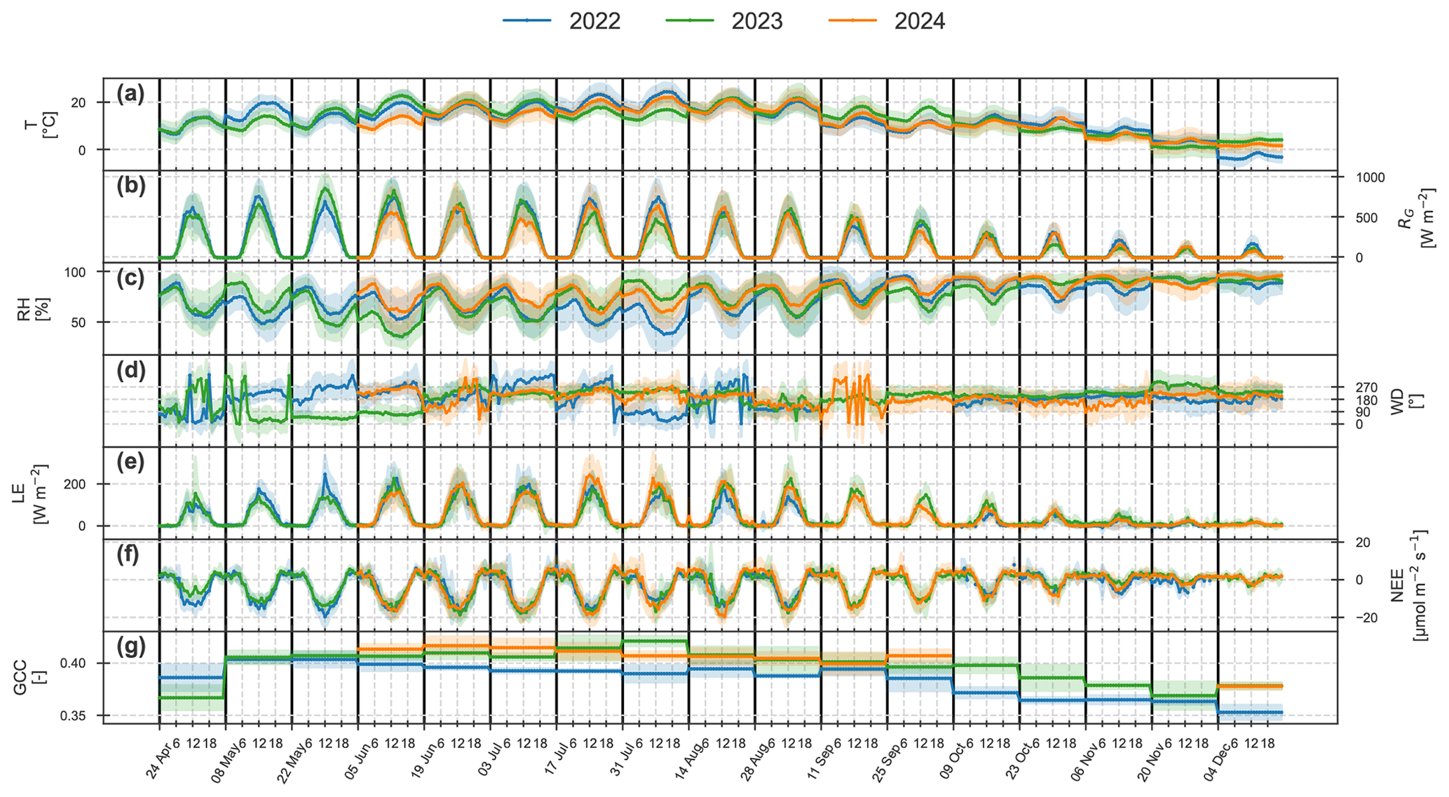
Figure 5 Average diel patterns (in LT) of meteorological and phenological conditions for each 2-week period. Solid lines represent hourly means, and shaded areas indicate the standard deviation around the mean. (a) Air temperature. (b) Incoming global radiation. (c) Relative humidity. (d) Wind direction. (e) Latent heat flux. (f) Net CO₂ flux. (g) Greenness index. All variables were measured at the top of the flux tower (TOP system). The greenness index (GCC) was measured once per day, so no diel pattern is shown for this variable and a single mean is provided for each 2-week period.

In 2022, a heatwave that lasted 8 consecutive days was observed from 9 to 16 August. This period was characterized by higher temperatures and radiation compared to the other years, and by lower relative humidity, partly due to very low precipitation (data not shown). From early December of the same year, temperatures were consistently below 0 °C for an extended period of days – a phenomenon not observed in the other years.

The year 2023 was marked by the two hottest months ever recorded in Belgium (June and September). At the end of May and beginning of June, a month-long period of anticyclonic conditions brought warm and dry air from the north-east sector.

Latent heat and carbon fluxes followed the expected patterns for a mixed temperate forest. Photosynthesis (Fig. 5f) and transpiration (Fig. 5e) were enhanced by the increase in temperature and radiation during the transition from spring to summer. The evolution of GCC (Fig. 5g) served as a proxy for leaf expansion of European beech. A strong development of vegetation was observed between 24 April and 8 May. Visual inspection of images captured from the top of the flux tower indicated that budburst occurred around 28 April, with little variation between years. In 2022, the onset of leaf fall was estimated between 20 and 26 October. Warmer conditions in 2023 delayed leaf fall compared to 2022, with observations indicating a period between 2 and 8 November. Phenological images were not available for 2024 to determine the leaf fall period.

3.2 Diversity of VOCs

3.2.1 Number of detected VOCs

In total, 74 $m/z$ values were retained by the DBSCAN algorithm. These ion species are listed in Table S3, along with their chemical formula, tentative compound identification, and parameters related to sensitivity computation.

It is important to note that compounds can give rise to signals at multiple ion masses, which may correspond either to isotopes associated with the chemical formula, to ion species resulting from the fragmentation of nascent excited protonated molecules (i.e., fragment ions), or to protonated water-cluster adducts formed in the ionization region. When reporting total VOC fluxes or concentrations, it is crucial to consider only one ion per compound to avoid double counting.

In general, water clusters and isotopes were not taken into account and have been excluded when compiling the list of ion masses considered (Table S3). One notable exception is protonated benzene ($m/z$ 79.054), whose peak is entangled with that of protonated hydrated acetic acid ($m/z$ 79.039). This entanglement is reduced for the ¹³C isotopes of these ion species (at $m/z$ 80.042 and 80.058, respectively) due to the relatively higher abundance of the protonated benzene isotope. As a result, only the protonated benzene isotope signal was considered for benzene quantification, eliminating any risk of double counting.

In contrast, both protonated molecules and their fragment ions are listed in Table S3 and were included in the concentration and flux database. Keeping both the protonated molecules and their corresponding fragments can be particularly informative, as temporal variations in their relative abundances can reveal shifts in chemical processes, ionization conditions, or source contributions. However, in the analyses and figures that follow, only one signal was taken into account for each VOC to avoid double counting and redundancy. To ensure the best possible quantification, we used the ion signal at the $m/z$ associated with the highest H₃O⁺/VOC product ion yield (Table S3), ending up with a list of 62 VOCs. It should be noted, however, that each of these reported VOCs represents a group of one or more individual chemical compounds contributing to the same $m/z$ signal, as listed in Table S3, and to which a single experimentally determined or estimated sensitivity factor was assigned. Consequently, when referring to the number of VOCs throughout this study, this number should be interpreted as the number of $m/z$-based VOC groups rather than the exact number of distinct molecular species exchanged by the ecosystem.

From these 62 VOCs, 44 were identified as significantly exchanged at the top of the tower, based on the three-step comparison of fluxes with LOD_f described in Sect. 2.3.5. The algorithm performed well in identifying ions with clear flux dynamics, with only a few exceptions: one VOC was found by the algorithm but displayed erratic flux patterns ($m/z$ 97.028 (C₅H₄O₂H⁺)), while five others exhibited consistent diurnal trends but were not detected by the algorithm – $m/z$ 97.065 (C₆H₈OH⁺), 99.044 (C₅H₆O₂H⁺), 101.023 (C₄H₄O₃H⁺), 103.075 (C₅H₁₀O₂H⁺), and 115.075 (C₆H₁₀O₂H⁺). The latter were manually included, and the former excluded, resulting in a final list of 48 VOCs considered significantly exchanged for the TOP system.

In summary, the DBSCAN algorithm retained 74 $m/z$ values corresponding to 62 VOCs, of which 48 showed significant exchange. This number is intermediate in comparison to other studies using a PTR-ToF-MS instrument. Some reported hundreds of ions with significant fluxes: 494 over an orange orchard in California (Park et al., 2013a); 377 above a mixed temperate forest in the USA (Millet et al., 2018); around 200 with a PTR3-ToF-MS above a boreal forest in Hyytiälä, Finland (Fischer et al., 2021); and 123 over a winter wheat field in France (Loubet et al., 2022). In contrast, other studies reported lower numbers than in the present work: 29 in a deciduous forest in Northern Italy (Schallhart et al., 2016); between 10 and 20 over a similar forest in the same region (Jensen et al., 2018); 25 above a boreal forest in Finland (Schallhart et al., 2018); and 18 compounds distributed over 43 ion species at a grassland site in Austria during harvest (Ruuskanen et al., 2011).

These large differences can be explained by the sensitivity of the PTR-ToF-MS instrument but also by the ecosystem type – for example, an orange orchard may emit substantially more VOCs than a temperate forest (Loubet et al., 2022). However, even for similar ecosystems and climatic conditions, Millet et al. (2018) reported six times more significant compounds than in the present study. This raises questions not only about instrumental performance, but also about the methodological choices involved in filtering ions to identify VOC exchanges.

Differences across studies already arise upstream of flux calculations, at the level of ion detection and selection. The number of ions identified by PTR-ToF-MS can vary substantially depending on how fragments, water clusters, isotopes, impurities, and other artefacts are filtered, a process that is often insufficiently described in the literature. In the present work, beyond an initial filtering of water clusters and isotopes, the application of the PAP software further reduced the ion list by retaining only mass-to-charge ratios for which peaks were regularly observed and generally above the limit of quantification.

At a later stage, when computing fluxes, additional methodological choices are introduced, particularly regarding the definition of a flux as being significantly different from zero. While most studies estimate the random flux error from the cross-covariance between vertical wind fluctuations (w^′) and concentration fluctuations (c^′) at large time lags – where the remaining covariance is attributed to noise (Langford et al., 2015) – the criteria used to extrapolate this assessment over an entire measurement period vary widely. Some illustrative examples are discussed below.

Loubet et al. (2022) computed an average random error following the recommendation of Langford et al. (2015), as the square root of the summed squared individual errors divided by the number of records. With this approach, the average random error decreases proportionally to $\mathrm{1}/\sqrt{n}$ when averaging over n measurements. Consequently, the longer the measurement period, the more likely a compound’s mean flux is to exceed its detection limit. Figure S15 compares the flux signal-to-noise ratios (SNRs, defined as the mean flux divided by the average error) reported in several PTR-ToF-MS studies for a subset of masses calibrated in the present study. For consistency, the SNRs shown for this work were computed using an average error calculated following Loubet et al. (2022). When averaging over our three measurement campaigns, the strong reduction in random error leads to SNRs that exceed those found in all other studies. In contrast, the lower SNRs in Park et al. (2013a), Ruuskanen et al. (2011), and Fischer et al. (2021) likely reflect the much shorter duration of their measurement periods. Applying the methodology of Loubet et al. (2022) to the present dataset would therefore lead to the conclusion that all 74 detected ions exhibit a mean flux significantly different from zero. This does however not necessarily imply that the exchange of a given VOC displays a clear, consistent, or interpretable temporal pattern.

Several alternative approaches have been proposed to identify significant VOC exchanges. For instance, Ruuskanen et al. (2011) visually assessed the quality of the covariance function (presence of a distinct and well-defined extremum) for each ion. While this approach was feasible for their 8 d measurement period, it becomes impractical and excessively time-consuming for longer measurement campaigns. Similarly, Fischer et al. (2021) selected compounds based on their covariance with the vertical wind component, although the exact evaluation criteria were not detailed. A more formalised approach was introduced by Park et al. (2013a), who computed a mean absolute covariance function from individual half-hourly records and compared its peak value to the standard deviation of the mean covariance function at large lag times, assumed to represent random noise. This framework provides a direct way to extrapolate half-hourly significance assessments to longer time periods. However, unlike the algorithm applied in the present study, such methods may fail to detect compounds that exhibit significant exchanges only during limited or episodic periods.

Among the diversity of existing methods, it is also worth highlighting the approach developed by Millet et al. (2018), who estimated the flux detection limit using an internal standard (diiodobenzene), for which no biogenic exchange is expected. Any measured flux of this compound can therefore be attributed to instrumental or internal effects – primarily fluctuations in relative humidity – and used to define a general detection limit.

Overall, the choice of detection and significance criteria has a direct and often dominant impact on the number of VOCs reported as being exchanged by an ecosystem (Schallhart et al., 2016; Jensen et al., 2018). The wide diversity of methodologies currently in use makes quantitative comparisons across studies challenging. We therefore advocate for the development of more unified algorithms and community standards for PTR-ToF-MS flux analyses.

For the TRUNK fluxes, only 31 $m/z$ values were identified as significantly exchanged. Considering their lower temporal resolution (about one half-hour every 2 h), and less pronounced flux dynamics, no visual inspection was applied to adjust this list.

3.2.2 Orders of magnitude

The mass range of the ion species used for the quantification of the 62 detected VOCs, as well as the range of their average mixing ratios and mean absolute fluxes, are illustrated in Fig. 6. It must be noted that in this study, VOC fluxes are reported in mass units (µg m⁻² s⁻¹), allowing for straightforward aggregation and carbon budget assessments. For fragment ions, molar fluxes were converted to mass units using the molar mass of the corresponding VOC.

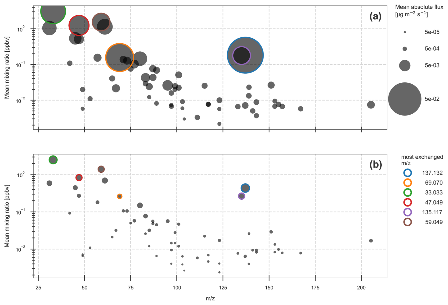
Figure 6 Mean mixing ratio of the 62 detected VOCs over the whole campaign (in log scale) as a function of the mass-to-charge ratio ($m/z$) of the ion species used for their quantification. (a) TOP system. (b) TRUNK system. For each $m/z$, the circle size is weighted by the corresponding absolute mean flux. The eight most exchanged ions (in terms of absolute mean flux) are highlighted on the graph.

The PTR-ToF-MS instrument was able to detect and quantify protonated VOCs with mass-to-charge ratios ranging from 31.018 (formaldehyde) to 205.195 (sesquiterpenes). In terms of average mixing ratios, concentrations span several orders of magnitude from approximately 3 ppbv for methanol down to pptv level for the least abundant compounds. Mixing ratios measured at the TRUNK level remain in the same range, although somewhat smaller than the ones acquired at the top of the flux tower. The top-left area of Fig. 6 is occupied by low molecular weight oxygenated compounds which are listed in Table 3: methanol ($m/z$ 33.033), acetic acid ($m/z$ 61.028), acetone ($m/z$ 59.049), ethanol ($m/z$ 47.049), formaldehyde ($m/z$ 31.018), formic acid ($m/z$ 47.013), and acetaldehyde ($m/z$ 45.033). These present the highest mixing ratios, across all seasons, although lower in autumn.

Table 3 Seasonal mean fluxes and concentrations of VOCs and ozone measured at the TOP system during 2022, 2023, and 2024. Only the 48 VOCs exhibiting significant exchange are reported and listed in descending order of flux magnitude. A tentative compound attribution is provided for ions with relatively high confidence. For others, candidates are listed in Table S3. For VOCs quantified based on their fragment ion, the chemical formula of the protonated compound is indicated. Compounds calibrated with a gas standard are indicated in italics. Note that ozone fluxes are reported in nmol m⁻² s⁻¹ as in the rest of the manuscript, while VOC fluxes were transformed from µg m⁻² s⁻¹ to ng m⁻² s⁻¹ to improve scaling.

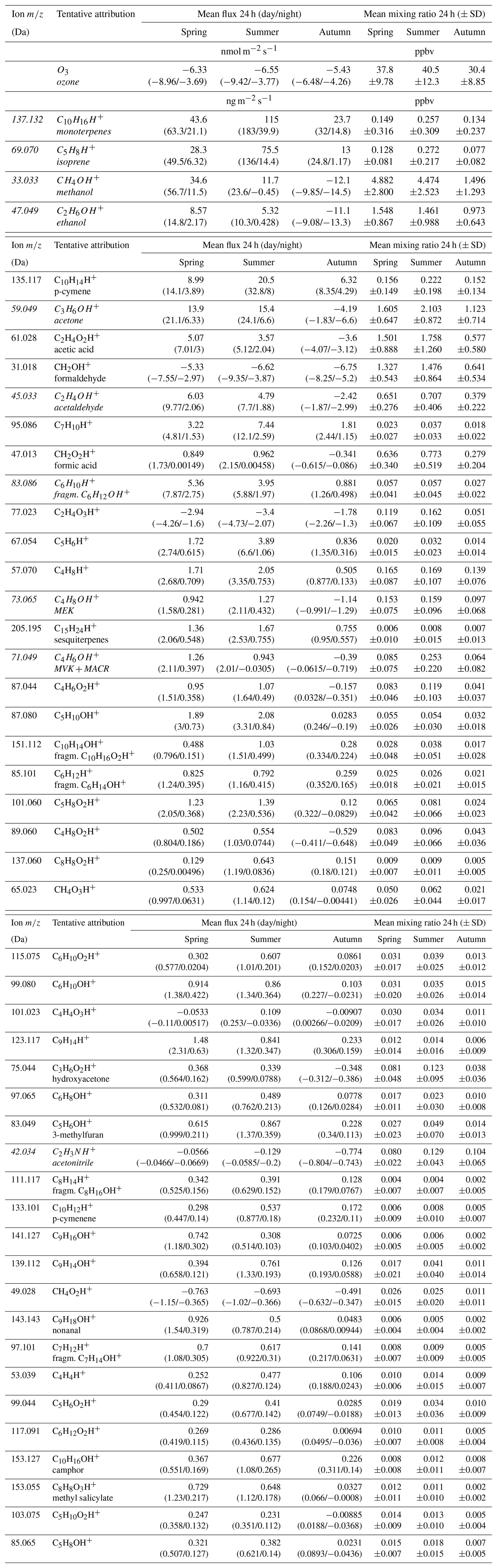
VOC concentrations show a clear decreasing trend with increasing $m/z$, both above the canopy (TOP system, Fig. 6a) and near ground level (TRUNK system, Fig. 6b). This pattern largely reflects the tendency for heavier compounds to exhibit lower volatility, which limits their ability to remain in the gas phase and accumulate in the atmosphere. Additionally, higher reaction rate constants with atmospheric oxidants contribute to the reduced concentrations of heavier BVOCs.

Local emissions also influence this pattern, as suggested by the circle sizes. Most of the strongest emissions correspond to ions with $m/z$ values below 80, while heavier compounds tend to show weaker emissions. Despite the overall trend, some compounds deviate from the expected decrease, exhibiting higher concentrations than those associated with neighbouring $m/z$ values. Notable examples include $m/z$ 137.132 (sum of monoterpenes) and $m/z$ 135.115 (C₁₀H₁₄H⁺, potentially p-cymene). These anomalies are associated with high fluxes, indicating an effect of local emissions on ambient VOC concentrations.

The seasonal dynamics of VOC ambient concentrations and fluxes will be further described in Sect. 3.3 and 3.4, respectively.

3.3 Ambient concentrations

Although the present study focuses on biogenic VOC and ozone exchange, the analysis of ambient concentrations provides valuable insights into some of the mechanisms driving the observed fluxes. Among the many measured compounds, a selection of chemical species with characteristic diel patterns is presented in Fig. 7. These exhibit pronounced cycles, albeit with differing phases and amplitudes, likely reflecting distinct sources, sinks, and reactivity. In addition, these patterns are modulated by atmospheric stability within the boundary layer, which influences vertical mixing and the vertical distribution of compounds. Their concentration profiles may therefore help identify sources and sinks at different heights, as well as the role of boundary-layer dynamics.

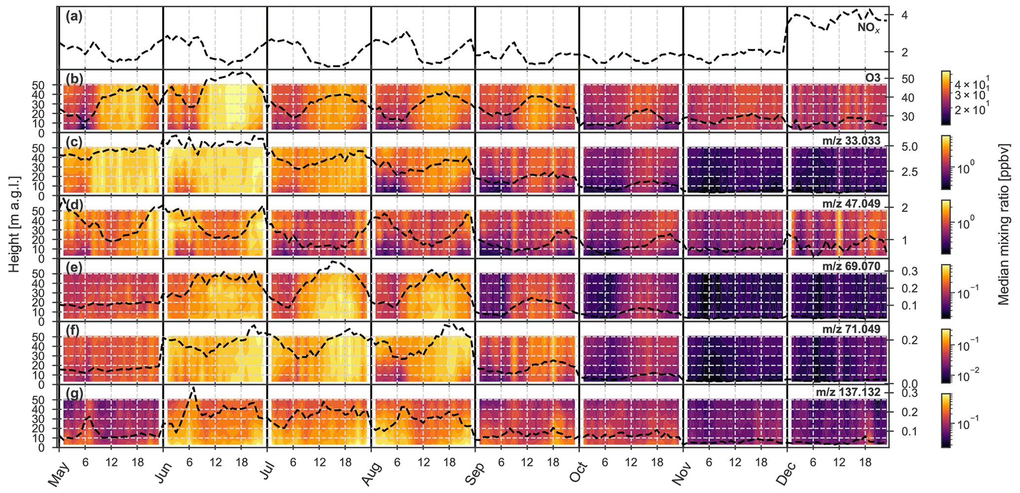
Figure 7 Average diel evolution (in LT) of vertical concentration profiles of selected trace gases for each month of the 2022, 2023, and 2024 field campaigns. (a) Nitrogen oxides (NO + NO₂). (b) Ozone. (c) Methanol. (d) Ethanol. (e) Isoprene. (f) MVK + MACR. (g) Sum of monoterpenes. Median values of 1 h aggregated data were computed, then interpolated horizontally (over time) and vertically (over height). The dashed line represents the median concentration measured at the TOP system.

Across seasons, average ozone concentrations ranged between 20 and 60 ppbv (Fig. 7b), consistent with values reported by Vermeuel et al. (2021) in a mixed temperate forest. Concentrations peaked in summer (June) and reached a minimum in autumn. This seasonal behaviour, along with the intra-daily variations described below, supports the photochemical origin of tropospheric ozone, which depends on solar radiation and temperature (Pellegrini et al., 2007). During the day, O₃ mixing ratios increase progressively after sunrise and peak in mid-afternoon (typically 16:00–18:00 LT), driven by photochemical production involving NO₂ photolysis and reactions with biogenic VOCs (Stockwell and Forkel, 2002; Faiola et al., 2024). After peaking, concentrations decline steadily towards the evening, as photochemical production decreases with declining solar radiation, and due to titration by NO, along with ongoing deposition. In a maritime pine forest, Kammer et al. (2018) observed nighttime ozone levels dropping below the detection limit (0.5 ppbv), suggesting efficient removal by highly reactive and abundant BVOCs. A similar phenomenon was reported by Andersen et al. (2024), but attributed to thermal inversion, which limited ozone replenishment from above; in this case, chemical loss alone was considered insufficient to explain the low nighttime ozone levels. In the present study, however, nighttime O₃ levels remained relatively high (on average between 10 and 20 ppbv).

Ozone concentrations were generally lowest near the ground, as observed by Petersen et al. (2023) in a boreal forest. Vertical stratification was especially evident in the morning and evening, when atmospheric mixing was reduced. The decrease near ground level may be attributed to continuous deposition from the canopy top downward (Zhou et al., 2017a), which was also observed at night in this study (Sect. 3.5). Furthermore, reduced photochemical production due to radiation attenuation within the canopy likely contributes to lower ozone levels close to the ground during the day.

In contrast, NO_x concentrations (Fig. 7a) showed a nocturnal pattern, peaking at night and in early morning. This accumulation likely results from soil NO emissions (Min et al., 2014) in combination with a stable nocturnal boundary layer that limits vertical mixing. As NO_x measurements were conducted at the ISSeP station, vertical concentration profiles are not available in this dataset, preventing direct verification of this hypothesis. After sunrise, NO_x levels decrease rapidly due to oxidation and dilution, occurring concurrently with ozone production. The amplitude of average NO_x concentrations ranged from 0 to a maximum of 5 ppbv, confirming the rural character of the site, with limited seasonal variation except in December, when peak values were observed – possibly due to reduced NO₂ photolysis or increased wintertime anthropogenic NO emissions.

Although chemically distinct from NO_x, many VOCs displayed similar diel behaviour, characterized by nighttime accumulation followed by a daytime minimum. These include ethanol ($m/z$ 47.049) as well as heavier masses, with the following potential attribution: $m/z$ 107.086 (xylenes), $m/z$ 121.101 (trimethylbenzene), $m/z$ 133.101 (p-cymenene), $m/z$ 135.117 (p-cymene), $m/z$ 143.143 (nonanal), and $m/z$ 153.127 (camphor). This pattern is illustrated for ethanol in Fig. 7d. The observed nighttime increase may reflect emissions under limited mixing conditions, supported by the stratification observed in vertical profiles. The daytime decrease, however, is more difficult to interpret, especially given the upward fluxes of ethanol measured during the day (Fig. 8d) and its relatively low reactivity (estimated atmospheric lifetime of 2.8 d, Naik et al., 2010). One possible explanation is that background concentrations are sufficiently high that local emissions do not result in noticeable concentration increases.

Figure 8 Seasonal evolution of VOC fluxes measured by the TOP system over the years 2022 (a–e), 2023 (f–k), and 2024 (l–o). For each $m/z$ value and hour of the day (in LT), mean fluxes are calculated only when at least 25 % of the expected half-hourly data are available within the corresponding period. The 10 most exchanged $m/z$ values are shown individually (see legend), while the remaining compounds are grouped into emission (“other > 0”) and deposition (“other < 0”) categories. Subplots aligned vertically correspond to the same seasonal period and share identical y axis limits to allow for direct visual comparison. The same figure with variable y axis is available in Sect. S3.8 for a distinct type of visualization.

In contrast to ethanol, methanol concentrations increased after sunrise (around 06:00 LT) and peaked in the evening before declining at night (Fig. 8c). The diel patterns of both OVOCs are broadly similar, but offset in time. This timing difference may arise from differing emission dynamics – methanol being among the most strongly exchanged VOCs (Table 3) – and differences in atmospheric reactivity (methanol's estimated lifetime of 4.7 d, Millet et al., 2008). Both compounds also showed decreasing vertical concentrations from above-canopy to ground level at night.

Methanol and ethanol concentrations were highest in May, whereas isoprene (Fig. 8e), methyl vinyl ketone (MVK) and methacrolein (MACR) (Fig. 8f), and monoterpenes (Fig. 8g) peaked in June, July, and August. These differences likely reflect distinct emission processes, further discussed in Sect. 3.4.

Isoprene and its oxidation products (MVK + MACR) exhibited diurnal profiles similar to that of ozone. Isoprene concentrations followed the expected light- and temperature-dependent emission patterns (Guenther et al., 2012), but showed a slight delay compared to solar radiation and isoprene fluxes. Peak concentrations typically occurred in the early afternoon (between 13:00 and 16:00 LT), whereas incoming radiation peaked around noon, isoprene fluxes near 13:00 LT, and air temperature somewhat later (15:30–16:00 LT). This pattern suggests that isoprene emissions (fluxes) closely track solar radiation, while atmospheric concentrations respond with a delay of a few hours following emissions. Vertically, maximum isoprene concentrations were not observed at the top of the flux tower (51 m a.g.l.) but rather near the canopy top, around 31 m a.g.l., indicating that emissions were primarily localized within or just above the canopy. From November onward, isoprene concentrations declined sharply, consistent with the strong seasonality of its emissions.

MVK + MACR differed from isoprene in timing and vertical distribution. Their concentrations peaked approximately 0 to 3 h after those of isoprene, consistent with their secondary formation through isoprene oxidation (estimated isoprene lifetime of ∼ 1.4 h, based on an average daytime OH concentration of 2×10⁶ molec. cm⁻³; Jensen et al., 2018). While isoprene concentrations were highest near the top of the canopy, MVK and MACR peaked slightly higher, around 51 m a.g.l., near the top of the measurement profile. This vertical offset may reflect enhanced isoprene oxidation above rather than inside the canopy.

Finally, monoterpenes displayed less pronounced diel patterns compared to the other species. Their emissions, which are predominantly temperature-driven (Guenther et al., 2012), also occurred at night. This may contribute to the lower diel variability in their mixing ratios relative to isoprene. Uniquely, monoterpenes reached maximum concentrations near ground level, a pattern also observed in a boreal forest by Petersen et al. (2023). This could reflect continuous nighttime emissions that accumulate within a shallow nocturnal boundary layer. Around sunrise (06:00–07:00 LT), concentrations increased at higher levels, possibly due to the onset of turbulent mixing.

While the above interpretations offer plausible explanations for the observed diel and vertical patterns, they remain limited by the complexity of the processes involved. In particular, ambient concentration dynamics results from the interplay between emissions, depositions, atmospheric transport, and chemical transformations. Disentangling the different factors affecting this type of dataset requires either methods to isolate specific features or more integrative approaches. For instance, to isolate where sources/sinks are located within the forest canopy, one can use Lagrangian modelling in combination with vertical concentration and turbulence profile measurements (Karl et al., 2004a; Tiwary et al., 2007; Wada et al., 2020; Petersen et al., 2023). Source apportionment studies can identify the impact of specific sources on local concentrations by using positive matrix factorization (Song et al., 2024), by looking at how meso-scale transport affects the concentration dataset (Simon et al., 2023), or by using a combination of both (Verreyken et al., 2021). The disadvantage of matrix factorization is that chemical degradation is not explicitly taken into account. To overcome this, chemically aged masses related to a specific source can be designated as separate factors and ageing regarded as a linear combination between both (Verreyken et al., 2021; Song et al., 2024). To identify the impact of chemistry on trace gas concentrations, one can use atmospheric chemistry models in various setups. Simple 0-D chemistry models can quantify chemical losses occurring at a specific site (Andersen et al., 2024). However, when characterizing a forest canopy, more integrative 1-D canopy exchange models (Ashworth et al., 2016; Zhou et al., 2017b) better represent the various processes occurring in the ecosystem. Unfortunately, 1-D canopy exchange models often neglect or strongly simplify the effect of advection of plumes originating from sources outside the forest. To get a broader picture of chemistry processes, the use of 3-D chemistry and transport models (Poraicu et al., 2025) are valuable tools for constraining the regional BVOC budget. However, they often lack a detailed representation of forest canopy structure, which can limit their accuracy in simulating in-canopy mechanisms. Altogether, combining multiple approaches remains essential to fully capture the complexity of trace gas dynamics within and above forest canopies.

3.4 VOC fluxes

3.4.1 Flux balance

BVOCs can both be emitted by the ecosystem (positive fluxes) and removed from the atmosphere through deposition (negative fluxes) via different biological, physical and chemical pathways. The total ecosystem exchange resulting from the balance between these two processes is illustrated in Fig. 8, across six representative 2-week periods. Note that only the 62 unique ions, representing each a single VOC, were considered in this figure to avoid skewing the mass balance. The description below focuses first on the year 2023, for which the measurement coverage was the most continuous.

Seasonal variability

During spring and summer, the net BVOC exchange was largely dominated by emissions (Fig. 8f–h), with a peak in mid-June (Fig. 8h), reaching a maximum mean value of ∼ 1.25 µg m⁻² s⁻¹ – more than three times higher than in May. Similar magnitudes were observed in July and August (not shown, but comparable to Fig. 8h). These maxima correspond to ∼ 0.9 µg C m⁻² s⁻¹ (carbon mass basis) or ∼ 18 nmol m⁻² s⁻¹ (molar basis). This value is twice as high as the summed flux of 494 detected ions in an orange orchard in summer (Park et al., 2013a). This difference is attributed to isoprene and monoterpenes, which contributed to most of the exchange in the present study while being very low in the orange orchard. Our maximum total flux of 18 nmol m⁻² s⁻¹ is closer to ranges reported by Schallhart et al. (2016) in a Mediterranean oak-hornbeam forest (between 25 and 30 nmol m⁻² s⁻¹), where isoprene emissions were dominant and much higher.

Expressing VOC fluxes on a carbon mass basis can be useful for assessing their contribution to atmospheric carbon. For comparison, daytime CO₂ uptake was about 20 µmol m⁻² s⁻¹ which is equivalent to 240 µg C m⁻² s⁻¹, such that the fraction of photosynthesized carbon allocated to VOC emission represented approximately 0.37 %. This fraction was highest in summer (daily median of up to 0.9 %) and lowest in autumn and winter (daily median of ∼ 0.1 %, data not shown here), consistent with observations reported for other vegetation types (Sharkey and Loreto, 1993; Peñuelas and Llusià, 1999, 2001). This summertime increase has previously been attributed to a potential acclimation strategy to cope with stressful conditions under high temperature and irradiance. The fraction of carbon allocated to VOCs was highest during the heatwave event encountered at BE-Vie, although not significantly higher than during the rest of the summer.

From September onward, the observed net fluxes decreased and approached a balance between emissions and depositions (Fig. 8i and j). This seasonal transition is attributed both to meteorological factors – namely decreasing temperature and solar radiation, which are key drivers of BVOC production – and to phenological changes such as vegetation senescence. Although Fig. 8 might suggest that downward fluxes were enhanced in autumn, they varied little across seasons and remained close to −0.1 µg m⁻² s⁻¹ or −0.05 µg C m⁻² s⁻¹ or −2 nmol m⁻² s⁻¹. These seemingly constant depositions are probably the result of compensating mechanisms. Lower mixing ratios and reduced stomatal aperture in autumn compared to spring (Fig. 7) would be expected to decrease stomatal VOC uptake (Niinemets et al., 2014). However, higher autumn humidity may enhance the deposition of water-soluble VOCs onto canopy water films followed by a (bacterial) consumption process (Laffineur et al., 2012), potentially compensating for the reduced stomatal uptake. This implies that downward VOC fluxes are less sensitive to seasonal variation than emissions, though a comprehensive modelling approach is needed to disentangle these effects.

Diurnal variability

At the diurnal scale, transitions from net uptake during the night to net release during the day are also evident. This diel pattern was particularly clear at the start of the 2023 campaign (Fig. 8f). During the night and early morning, depositions were observed for small oxygenated compounds such as methanol ($m/z$ 33.033), ethanol (47.049), acetone (59.049), acetic acid (61.028), acetaldehyde (45.033), and formic acid (47.013). As shown in Fig. 5c, humidity was higher at night, creating conditions favouring the adsorption of such compounds on water films. Higher concentrations found at night (Fig. 7) could also have induced downward fluxes, although stomatal closure exerts a strong control on the stomatal sink. At night, isoprene flux ($m/z$ 69.070), which is light-dependent, was not detected in the absence of solar radiation. In contrast, temperature-driven compounds such as monoterpenes ($m/z$ 137.132) and $m/z$ 135.117 (C₁₀H₁₄H⁺, potentially p-cymene) were still emitted at night, as illustrated in Fig. 8i and j.

From around 07:00 LT, total emissions increased, primarily driven by monoterpenes and isoprene, which were the dominant daytime BVOC sources in this ecosystem. Concurrently, net fluxes of small oxygenated BVOCs switched from negative to positive shortly after sunset. Niinemets et al. (2014) describes this transition as the result of the outgassing of VOCs from water films to the gas phase and stomatal opening. However, it is important to note here that the eddy covariance technique provides net exchange measurements; hence, this shift does not imply the absence of deposition, but rather that emission rates surpass deposition. This bidirectional behaviour – nighttime net uptake followed by daytime net release – has been previously documented (Millet et al., 2018; Schallhart et al., 2016) and confirms the existence of two-way exchange mechanisms. Compounds exhibiting this pattern are referred to as “bidirectional BVOCs”. Their relative contribution was particularly high in May, following the canopy leaf-out. In Fig. 8g, methanol emissions even exceeded those of isoprene and monoterpenes, which may reflect leaf expansion, as methanol is known to be produced by pectin demethylation during cell wall expansion (Kreuzwieser, 2002; Wohlfahrt et al., 2015). After the summer, these compounds generally reverted to net deposition over the full day.

VOC acting as a net sink

Among all of the detected VOCs, formaldehyde was the only compound presenting downward fluxes at all seasons and every hour. However, one should note that the quantification of formaldehyde concentrations and fluxes comes with high challenges and uncertainties. Protonated formaldehyde can undergo back reactions with water vapour in the PTR-ToF-MS instrument (Inomata et al., 2008), making its quantification sensitive to relative humidity. In the present study, the sensitivity of our PTR-ToF-MS to formaldehyde was estimated from a comparison with HPLC analyses performed during the EMEP2022 campaign (Fagerli et al., 2023 and Sect. 2.5.1), which resulted in a very good correlation. However, this comparison was made over samples taken during 6 warm days in July. The estimated sensitivity does therefore not take different classes of relative humidities into account. This humidity-dependent sensitivity can lead to fluctuations in high-frequency data which skew fluxes computed with the EC technique. Loubet et al. (2022) estimated that the impact of water vapour variations on fluxes was negligible for most VOCs except formaldehyde, which should be considered with caution. The same advice is given in the present study.

Relative VOC contribution

BVOCs not individually represented in Fig. 8 still contributed substantially to the overall flux (see the “other > 0” and “other < 0” categories). In summer, between 15 and 20 species were required to capture 90 % of the total upward flux expressed in carbon mass units. In comparison, Millet et al. (2018) found that only 5 ions were sufficient to represent 90 % of the summed emissions in July, despite considering 377 ions in the total flux. In both cases, this indicates that strong emitters are followed by a long tail of VOCs with very low upward fluxes, although this phenomenon is more pronounced in Millet et al. (2018). In autumn, 30 compounds were needed to capture 90 % of the total upward flux, as the relative importance of the top emitters (isoprene, monoterpenes) decreased. To account for 90 % of the summed depositions, between 30 and 43 compounds were necessary. This confirms the observation by Millet et al. (2018) that the total deposition flux is composed of a larger number of species with lower individual contributions.

Vermeuel et al. (2023a) expanded the suite of VOCs measured over a coniferous forest by combining PTR-ToF-MS with iodide chemical ionization mass spectrometry (ICIMS) flux measurements. While upward fluxes of VOC species detected with PTR-ToF-MS and included in CTMs were accurately simulated by GEOS-Chem, many additional species not represented in CTMs contributed significantly to the total downward VOC flux. This led to an underestimation of the reactive carbon sink by GEOS-Chem. Notably, downward fluxes of VOCs detected by PTR-ToF-MS alone accounted for only 63 % of the total deposition, indicating that 37 % would have been missed without the inclusion of ICIMS measurements. The compounds missed without ICIMS include oxidation products of isoprene and of 232-MBO, as well as > C₂ organic acids. These findings suggest that the results presented in the present study may underestimate part of the total VOC deposition.

Inter-annual variability

The seasonal and diel trends described for 2023 were also observed in 2022 and 2024, with some differences that can be attributed to varying meteorological conditions and the differing contributions of tree species to the measured fluxes (discussed in Sect. 3.4.2). In early May 2022, warmer and sunnier weather favoured stronger emissions compared to the same period in 2023 (Fig. 8a and b vs. Fig. 8f and g). Conversely, in June 2024, emission levels were much lower (Fig. 8l) than those in June 2022 (Fig. 8c) and 2023 (Fig. 8h) – a difference of nearly a factor of three – further highlighting the high sensitivity of BVOC fluxes to light and temperature. Notably, the relatively warm autumn conditions in 2024 sustained active emissions into early November (Fig. 8o), in contrast to 2023 where emissions did not show any clear dynamics (Fig. 8k).

Figure 9 Same as Fig. 8 but for TRUNK fluxes, over the years 2023 (a–f) and 2024 (g–h).

The maximum monoterpene flux observed in the present study (1.63 µg m⁻² s⁻¹) exceeded the value previously reported at the same site in 2009 using a PTR-Quad-MS (0.69 µg m⁻² s⁻¹) (Laffineur et al., 2011). In both cases, these maxima occurred under air temperatures exceeding 30 °C. From 2022 to 2024, only 0.1 % of the monoterpene fluxes exceeded the 2009 value of 0.69 µg m⁻² s⁻¹. In contrast, the maximum isoprene flux in the present study (1.18 µg m⁻² s⁻¹) was lower than in 2009 (1.96 µg m⁻² s⁻¹). Methanol was another compound reported in 2009 and 2010 (Laffineur et al., 2012). While the 24 h average maximum emissions were similar in both studies (approximately 0.07 µg m⁻² s⁻¹ in spring and 0.02 µg m⁻² s⁻¹ in summer), methanol deposition fluxes reported by Laffineur et al. (2012) were roughly twice those measured in the present dataset. Methanol concentrations, however, were comparable in both studies, and no unusual meteorological event was reported in 2009 or 2010 that could explain these differences. Given the many factors that may have varied between the two measurement periods – including vegetation type and cover, climatic conditions, and instrumental characteristics – it is difficult to draw firm conclusions based solely on the observed differences in monoterpene, isoprene, and methanol fluxes.

Below-canopy fluxes

Below-canopy fluxes measured by the TRUNK system exhibited a seasonal transition similar to that observed at the TOP level (Fig. 9). However, the net balance was already dominated by deposition at the beginning of the campaign (Fig. 9a). The dominant emissions observed in late spring and early summer (Fig. 9b and c) declined earlier and more steeply, resulting in a faster shift towards net deposition in subsequent periods (Fig. 9d–f).

Flux magnitudes (maximum diel values) were at least ten times lower than those observed at the top of the canopy, and across all periods. Maximum emission values rarely exceeded 0.06 µg m⁻² s⁻¹, reflecting the more limited production capacity below the canopy. Importantly, no additional significant BVOC signals appeared in the TRUNK data that were not already detected in the TOP dataset. This suggests that the same suite of compounds is involved in the exchange processes, albeit at reduced intensity.

The diurnal flux dynamics observed above the canopy were much less pronounced in the TRUNK system. A clear daytime emission peak was only visible in Fig. 9b and c, corresponding to late May and mid-June. During the remainder of the year, no systematic diurnal pattern emerged, suggesting that the below-canopy environment is governed by mechanisms other than those controlling foliar emissions. Isidorov and Zaitsev (2022) list a variety of biotic and abiotic drivers of leaf litter decomposition and soil-atmosphere VOC exchanges, many of which remain poorly characterized. Given the diversity of processes involved, a large variability in VOC exchanges measured near the ground is expected. Nonetheless, owing to its continuity and coverage of a wide range of environmental conditions, the present dataset may offer an opportunity to disentangle some of these (a)biotic controls.

Finally, we emphasize that TRUNK measurements do not solely represent soil and litter emissions, as some understorey vegetation (including young trees) was present below 3 m a.g.l. (Fig. 3). This vegetation may explain the daytime upward fluxes observed in Fig. 9b and c, which follow the evolution of temperature and light.

3.4.2 Flux dynamics

Figures 8 and 9 provide an overview of total BVOC exchange but do not highlight the specific temporal dynamics that could shed light on production and deposition mechanisms. A more detailed analysis of the flux time series allows for the identification of different categories of BVOCs based on their flux temporal behaviour. To illustrate these patterns, a selection of five $m/z$ values is presented in Fig. 10.

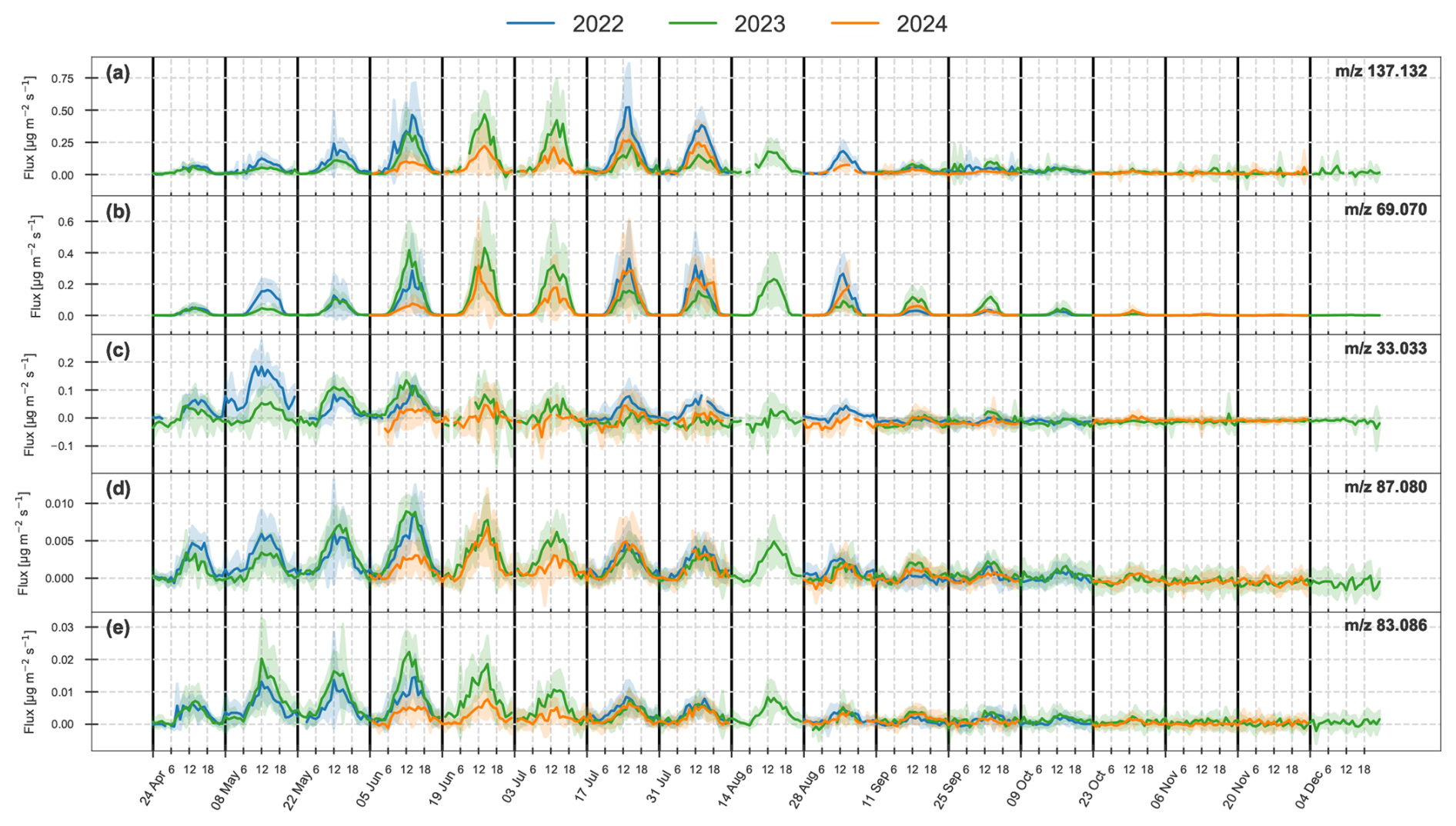
Figure 10 Average diel patterns (in LT) of BVOC TOP fluxes for each 2-week period. (a) Sum of monoterpenes. (b) Isoprene. (c) Methanol. (d) MBO. (e) C₆H₁₀H⁺. The five $m/z$ values shown exhibit distinct exchange behaviours. Solid lines represent hourly mean fluxes, and shaded areas indicate the standard deviation around the mean. For each 2-week period, the diel pattern is displayed only if data were available for at least 25 % of the expected hours.

Isoprene and monoterpenes (Fig. 10a and b) exhibit the clearest and least noisy flux signals. Another $m/z$ value associated with well-defined emissions is 153.055 (C₈H₈O₃H⁺, potentially methyl salicylate), although its flux magnitude is approximately 100 times lower (data not shown). As discussed previously, the emission of isoprene and monoterpenes peaked in summer, between 5 June and 14 August. Isoprene and monoterpenes showed similar flux magnitudes, but some differences are noteworthy. For instance, from 5 to 19 June, fluxes of monoterpenes were higher in 2022 than in 2023, whereas the opposite was true for isoprene. Temperature and radiation were comparable during this period in both years (Fig. 5), however, differences in the prevailing wind direction may partly explain the observed patterns. In 2022, winds predominantly originated from the south-west sector, where European beech was the dominant tree species, accounting for 62 % of the vegetation within the 70 % flux footprint (followed by 24 % of silver fir; Fig. 1). Measurements conducted in 2009 at the same site by Laffineur et al. (2011) identified European beech as the main monoterpene emitter among the species present at BE-Vie. The higher monoterpene emissions in 2022 appear to support this finding. In contrast, in 2023, winds mainly originated from the north-east sector, which was dominated by Norway spruce, representing 61 % of the vegetation within the 70 % flux footprint, followed by Douglas fir (17 %). The increased isoprene fluxes during that period suggest that Norway spruce may act as an isoprene emitter at BE-Vie, in line with the findings of Filella et al. (2007), although this could not be confirmed by Laffineur et al. (2011).

Another possible explanation for the increased emissions of $m/z$ 69.070 in 2023 compared to 2022 is provided by the signal at $m/z$ 87.080 (Fig. 10d), to which 2-methyl-3-buten-2-ol (MBO) may contribute. Between 22 May and 19 June, $m/z$ 87.080 also showed higher upward fluxes in 2023. MBO emissions have been reported from Norway spruce forests by Juráň et al. (2017), and since this compound is known to fragment at $m/z$ 69.070, the enhanced fluxes observed in Fig. 10b under winds from the Norway spruce sector may reflect MBO emissions. Interestingly, emissions at $m/z$ 87.080 developed earlier in the season than those of isoprene, and showed only limited variation throughout spring and summer. If MBO is indeed contributing to the signal at $m/z$ 87.080, this observation contrasts with the estimates from Guenther et al. (2012), which suggest similar light and temperature dependencies for both isoprene and MBO.

The differences in emission patterns observed between the 2 years, and their apparent link to prevailing wind directions and stand composition, illustrate the challenges and opportunities of working in a heterogeneous forest ecosystem. While such heterogeneity complicates the attribution of observed fluxes to specific sources, it reflects the reality of many temperate forests and is likely to become even more common as forest management moves away from monocultures towards more resilient, mixed-species stands (Seliger et al., 2023, and references therein). At BE-Vie, this heterogeneity is not evenly spread but rather organized in species-dominated patches. Future efforts to refine flux interpretation could build on the existing high-resolution tree species distribution map (Fig. 1) combined with footprint-weighted flux disaggregation approaches, to better attribute observed fluxes to their biogenic sources.

The methanol flux (Fig. 10c) is a clear example of the bidirectional behaviour typical of some BVOCs, with weak nighttime deposition followed by daytime emissions. Methanol fluxes rise earlier and more rapidly than those of isoprene or monoterpenes, peaking between 22 May and 5 June. This early increase and subsequent decline after 19 June likely reflect leaf development and cell expansion processes (Wohlfahrt et al., 2015).

In Fig. 10e, $m/z$ 83.086 (C₆H₁₀H⁺, potentially a fragment of hexenol or hexanal) exhibited an unexpected emission peak in 2023, between 8 and 22 May. This peak resulted from exceptionally high upward fluxes recorded over 2 d (9–11 May) and was also observed for other C₆–C₉ aldehydes and alcohols: $m/z$ 101.096 (C₆H₁₂OH⁺, likely protonated hexenol or hexanal), $m/z$ 143.143 (C₉H₁₈OH⁺, potentially nonanal), and two additional ions probably related to nonenal, $m/z$ 123.117 (C₉H₁₄H⁺) and $m/z$ 141.127 (C₉H₁₆OH⁺). These emission bursts were likely triggered by a hailstorm that occurred during this period in 2023, which caused significant canopy damage and left many broken branches and leaves on the forest floor. The above-mentioned ion species are commonly referred to as green leaf volatiles (GLVs) (Dudareva et al., 2013) and may have originated from wounded plant tissues – a well-documented source of GLV emissions (Scala et al., 2013; Niinemets et al., 2014). During this burst, the GLVs reached peak fluxes ranging from 18 times (for $m/z$ 101.096) to 37 times (for $m/z$ 123.117) their median positive fluxes, highlighting the substantial enhancement of their emissions under stress conditions.

3.5 Ozone fluxes

As expected, ozone fluxes were always negative, representing a net deposition into the ecosystem (Fig. 11). Unlike for VOCs, O₃ fluxes were expressed in molar units, which is a common practice, to directly reflect the number of molecules involved in atmospheric chemical reaction.

Figure 11 Same as Fig. 10 but for O₃ fluxes. (a) TOP system. (b) TRUNK system.

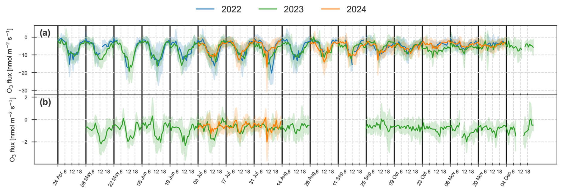
For the TOP system, O₃ depositions showed a clear diurnal pattern, with a maximum absolute flux found mostly around 11:00 and 12:00 LT. This evolution from nighttime to daytime depositions can be attributed to the stomatal aperture and subsequent ozone uptake, which is known as a major O₃ deposition pathway (Clifton et al., 2020). Average daytime ozone uptake rapidly increased from spring (8.96 nmol m⁻² s⁻¹) until reaching maximum values in summer (9.42 nmol m⁻² s⁻¹, Table 3). This reflects elevated O₃ concentrations (Fig. 7) and leaf development among deciduous species, which began in late April/early May. During summer, O₃ depositions varied to a small extent and started decreasing from October to reach 24 h-averaged fluxes of −5.43 nmol m⁻² s⁻¹ in autumn. Again, this is primarily due to the onset of leaf senescence – with leaf fall typically occurring in late November – combined with lower ozone levels in ambient air.

Nighttime depositions showed less variation than daytime ones (in terms of mean values and standard deviations). The non-zero values indicate a continuous uptake, even when stomata where closed. These nighttime fluxes remained relatively stable throughout the seasons compared to daytime depositions, although the phenology of the forest did evolve. This supports the idea of non-stomatal deposition pathways, such as uptake by leaf cuticles, soil and water (Clifton et al., 2020).

Overall, the inter-annual variability of TOP fluxes was limited. Daytime ozone uptake reached its highest mean value in 2022, with 20 nmol m⁻² s⁻¹ recorded during the fortnight from 31 July to 14 August, which coincided with a heatwave. Under such heat stress, stomatal conductance would normally be expected to decline, leading to reduced ozone uptake. The enhanced O₃ deposition observed here can be partly understood in light of the elevated ambient ozone levels recorded during the heatwave (above 70 ppbv). Moreover, Juráň et al. (2025) reported that during drought conditions, non-stomatal ozone fluxes compensated for reduced stomatal uptake in a temperate Norway spruce forest. The increased contribution of non-stomatal deposition was attributed mainly to reactions on leaf cuticles and on soil particles, and to a lesser extent to chemical loss through reactions with VOCs.

Below-canopy fluxes also exhibited a diurnal pattern, with an increase from non-zero nighttime depositions to maximum daytime depositions around 14:00 LT on average – later than observed for the TOP system. This delay may be attributed to ozone concentrations taking longer to rise after sunrise at the TRUNK level compared to above the canopy (Fig. 7), possibly due to delayed photochemical activity near the forest floor.

Both in 2023 and 2024, TRUNK fluxes rapidly declined from 3 July and remained in the same order of magnitude for the rest of the campaign. This contrasts with above canopy fluxes which maintained high deposition values and seemed more sensitive to meteorological and phenological conditions. The explanation for this decrease remains unclear. As a reminder, TRUNK fluxes were measured 3 m above ground level, and therefore primarily reflect non-stomatal deposition pathways, such as uptake by soil, litter, or water surfaces (Clifton et al., 2020). These processes would be expected to persist even during summer.

TRUNK fluxes represented on average approximately 10 % of the above-canopy fluxes, although large variations were observed – from 0 % to 50 %. This is broadly consistent with the range of 5 % to 39 % reported by Fares et al. (2014), and references therein. The relative contribution of TRUNK fluxes was often higher at night, in agreement with observations from the Landes forest by Lamaud et al. (2002), likely due to the reduced importance of stomatal deposition in the total ozone sink during the night.

In 2023, we observe a little boost of below-canopy O₃ uptake from 6 until 20 November. This period exactly coincides with the fall of dead leaves from deciduous trees. An explanation of this increased consumption might be linked to a reaction of ozone with compounds present on the surface of senescent and/or dead leaves. This phenomenon was observed both in situ and in vitro by Potier et al. (2015, 2017) and was attributed to ascorbate leaching out from senescent and dead leaves.

4 Code and data availability

Four distinct groups of datasets are available for the BE-Vie site during the 2022–2023–2024 period:

• i.

  Main measurements (present study). 1 min concentrations of VOCs and O₃ are available at https://doi.org/10.18758/NVFBA74V (Verreyken et al., 2025c); 30 min concentrations and fluxes (TOP & TRUNK) of VOCs and O₃ are available at https://doi.org/10.18758/KHV8ZXU2 (Dumont et al., 2025a); vertical profiles of VOC and O₃ concentrations and turbulence are available at https://doi.org/10.18758/BED4Q2VY (Dumont et al., 2025b).

• ii.

  ICOS measurements. Flux and meteorological data were downloaded from the ETC L2 ARCHIVE on the ICOS Carbon portal https://doi.org/10.18160/S6HM-CP8Q (Vincke et al., 2025).

• iii.

  ISSeP measurements. Data from the ISSeP air quality station were downloaded from the wallonair platform https://data.wallonair.be/ (last access: 13 January 2026. More information available upon request from b.bergmans@issep.be.

• iv.

  Remote-sensing measurements. Data available upon request from alexis.merlaud@aeronomie.be.

Results from the EMEP campaigns (VOC analysis by GC-MS and HPLC) will be made available through the EBAS data repository (http://ebas.nilu.no/, last access: 13 January 2026).

The Peak Area Processing software (PAP, used for non-targeted peak selection, instrument characterization, and quantification of mixing ratio's with related uncertainties) is available here: https://doi.org/10.18758/2i4h1353 (Verreyken et al., 2025a). A test dataset for the PAP software can be found here: https://doi.org/10.18758/BDBRICLK (Verreyken et al., 2025b). GEddySoft (software used to process VOC fluxes with the eddy covariance method) is available here: https://github.com/BernardHeinesch/GEddySoft (last access: 13 January 2026). A test dataset for GEddySoft can be found here: https://doi.org/10.18758/IYPN6FNM (Heinesch et al., 2025).

5 Conclusions

This study presents a 3-year field campaign (2022–2024) of VOC and ozone dynamics at the extensively instrumented ICOS forest station of Vielsalm (BE-Vie), combining a vertical profile with eddy covariance fluxes above and below the canopy. A new open-source processing pipeline (PAP and GEddySoft) was developed to quantify VOC mixing ratios and fluxes using a PTR-ToF-MS instrument. Various critical steps of the eddy covariance methodology applied to VOC and ozone flux measurements were addressed, including data quality flagging, storage corrections, sonic anemometer rotation within the trunk space, and ozone flux calibration.

The processing of VOC data resulted in the identification of 48 significantly exchanged VOCs among 74 VOC-related signals, based on a single representative ion $m/z$ per VOC and fluxes frequently exceeding the detection limit. These included both well-known biogenic VOCs and lesser-studied compounds, reflecting the chemical and functional diversity of VOC exchange in forest ecosystems. The number of significantly exchanged VOCs is intermediate in comparison to other studies using a PTR-ToF-MS instrument – while Park et al. (2013a); Millet et al. (2018); Fischer et al. (2021); Loubet et al. (2022) identified hundreds of compounds, others found tens of VOCs exhibiting significant fluxes (Ruuskanen et al., 2011; Jensen et al., 2018; Schallhart et al., 2018). Despite potential differences in ecosystem signatures and instrumental capabilities, this raises questions about the criteria used to determine whether a flux is considered significant or not.

Ambient mixing ratios revealed clear vertical and diurnal gradients shaped by the interplay of emission, deposition, photochemistry, and atmospheric transport. Ozone and NO_x exhibited tightly coupled patterns, with daytime O₃ formation and nighttime NO_x accumulation. VOCs showed compound-specific behaviour: ethanol remained relatively constant due to high background levels, methanol followed a daytime emission pattern, and isoprene peaked near the canopy with oxidation products (MVK + MACR) accumulating at higher altitudes. At night, monoterpenes accumulated near the forest floor, indicating sustained temperature-driven emissions and limited mixing. These observations highlight the value of high-resolution datasets for exploring the spatial and temporal dynamics of reactive trace gases within a forest ecosystem.

The forest acted as a net source of VOCs for most of the measurement period, with peak emissions in summer exceeding 1.25 µg m⁻² s⁻¹. Monoterpenes, isoprene, and methanol dominated the fluxes. However, between 15 and 30 compounds were needed to capture 90 % of the total emissions (depending on the season), and between 30 and 43 for deposition, confirming the importance of considering a broad range of compounds beyond a few dominant species. According to Vermeuel et al. (2023a), up to 37 % of the total downward flux of VOCs would be missed when relying on PTR-ToF-MS measurements alone. Therefore, while the upward fluxes reported in this study are likely representative of total ecosystem emissions, the total deposition should be regarded as a lower limit of the actual ecosystem sink.

The total VOC deposition remained relatively stable across seasons (∼ −0.1 µg m⁻² s⁻¹), while emissions showed stronger seasonal variability. Many oxygenated VOCs exhibited bidirectional behaviour, switching from nighttime deposition to daytime emission – especially in spring after budburst – underlining the importance of biological processes and environmental conditions.

The interannual variability in flux magnitudes – such as the markedly lower emissions observed in June 2024 compared to previous years – further emphasizes the sensitivity of VOC exchange to meteorological and phenological drivers. Fluxes measured near the forest floor were generally close to equilibrium between emissions and depositions, except in late spring and early summer, when upward fluxes increased.

Additional insights were gained into species-specific emission patterns, with wind direction modulating isoprene and monoterpene fluxes. For instance, Norway spruce was identified as a likely isoprene and MBO emitter at this site. A short-lived burst of green leaf volatiles following a hailstorm also illustrated the ecosystem’s capacity for rapid VOC responses to disturbance. The spatial heterogeneity of the forest, while challenging for flux attribution, also offers an opportunity to improve our understanding of species-specific emissions in realistic, mixed-species stands.

Ozone fluxes remained consistently downward, with the strongest uptake in spring and early summer. Below-canopy deposition accounted for ∼ 10 % of the above-canopy flux on average, although this ratio was variable. These patterns point to persistent non-stomatal uptake processes, both above and below the canopy, and suggest opportunities for further partitioning of ozone sinks.

Overall, this study provides one of the most detailed long-term characterizations of trace gas exchange in a temperate mixed forest. The diversity of behaviours observed across compounds, seasons, and canopy levels offers a unique dataset for the development and calibration of process-based models, including bidirectional biogenic, physical and chemical exchange schemes. Such models are essential for improving predictions of VOC–ozone–aerosol interactions and their feedbacks on air quality and climate.