Gulf of St. Lawrence and Estuary Dataset (GOSLED): a 20-year compilation of quality-controlled biogeochemical observations (2003–2023)

This paper presents the Gulf of St. Lawrence and Estuary Dataset (GOSLED), a quality-controlled compilation of biogeochemical observations collected during 21 research cruises in the St. Lawrence Estuary, Gulf of St. Lawrence, and Saguenay Fjord between 2003 and 2023. This dataset integrates hydrographic measurements and a broad suite of discrete biogeochemical variables into a single, standardized compilation suitable for reuse, synthesis, and long-term analysis. GOSLED includes discrete measurements of dissolved oxygen, carbonate-system parameters, macronutrients, dissolved organic carbon, selected biogeochemical gases, stable isotope ratios of carbon and water, and transient and deliberate tracers. Data were compiled from multiple independent research cruises and laboratory archives (2003–2020), including contributions from the Marine Environmental Observation, Prediction and Response Network (MEOPAR) – Réseau Québec maritime (RQM) Gulf of St. Lawrence Tracer Release Experiment (TReX; 2021–2023), RQM Odyssée Saint Laurent program (2018–2023), and the Fisheries and Oceans Canada (DFO) Atlantic Zone Monitoring Program (AZMP; fall 2022). Sampling was conducted predominantly during the ice-free season, resulting in limited winter coverage across much of the system. All data were harmonized and processed following primary quality-control procedures adapted from GLODAP and CODAP-NA standards. Secondary crossover analysis was not possible due to a lack of deep-water (>1500 m) sampling. This paper documents the data provenance, quality-control procedures, known limitations, and recommended considerations for dataset usage. GOSLED is archived at the Canadian Integrated Ocean Observing System – St. Lawrence Global Observatory (CIOOS-SLGO) and is publicly accessible at https://doi.org/10.26071/d6f3fdfc-788d-48ff (Nesbitt et al., 2026).

1 Introduction

High-quality, long-term, quality-controlled datasets are essential for the advancement of ocean and climate research, and for monitoring the temporal dynamics of biogeochemical variables. These variables form the backbone of long-term trend analyses, inform ecosystem health assessments for conservation and fisheries management, and support climate model projections that guide environmental policy. In estuaries and coastal seas, where anthropogenic nutrient loading, seasonal stratification, and long residence times are ubiquitous, biogeochemical data products are critical for capturing phenomena such as de-oxygenation and acidification that can constrict suitable aquatic habitats, alter trophic structure, and modulate microbial metabolic activity.

The Estuary and Gulf of St. Lawrence (EGSL) make up one of the largest semi-enclosed estuarine systems on Earth (Laruelle et al., 2024; see Fig. 1). Over the past century, the deep-layer dissolved oxygen (DO) concentrations at the head of the Lower St. Lawrence Estuary (LSLE) have declined from ∼125 µmol kg⁻¹ in ∼1930 (Gilbert et al., 2005; Jutras et al., 2020, 2023b) to as low as ∼25 µmol kg⁻¹ in 2022 (Blais et al., 2023; Jutras et al., 2023b), reaching a state of severe hypoxia that was still observed in 2024 (Blais et al., 2025). This long-term deoxygenation is driven by eutrophication and changes in the western North Atlantic circulation, particularly the reduced inflow of the cool, oxygen-rich Labrador Current Water (LCW) and the increasing dominance of the warm, oxygen-poor North Atlantic Central Water (NACW) through the Cabot Strait (Jutras et al., 2020, 2023b). Over the same period, the deep-layer pH has declined by ∼0.3–0.4 units due to the accumulation of metabolic CO₂ (Galbraith et al., 2025a; Mucci et al., 2011), leading to aragonite undersaturation throughout the EGSL and the emergence of calcite undersaturation in the LSLE (Galbraith et al., 2025a), threatening the viability of CaCO₃-secreting organisms and the preservation of their fossil remains (Mucci et al., 2011; Nesbitt and Mucci, 2021). Together, these processes have created a regional hotspot of severe hypoxia and ocean acidification with direct consequences for both pelagic and benthic habitats (Pascal et al., 2024), fisheries, and ecosystem functions.

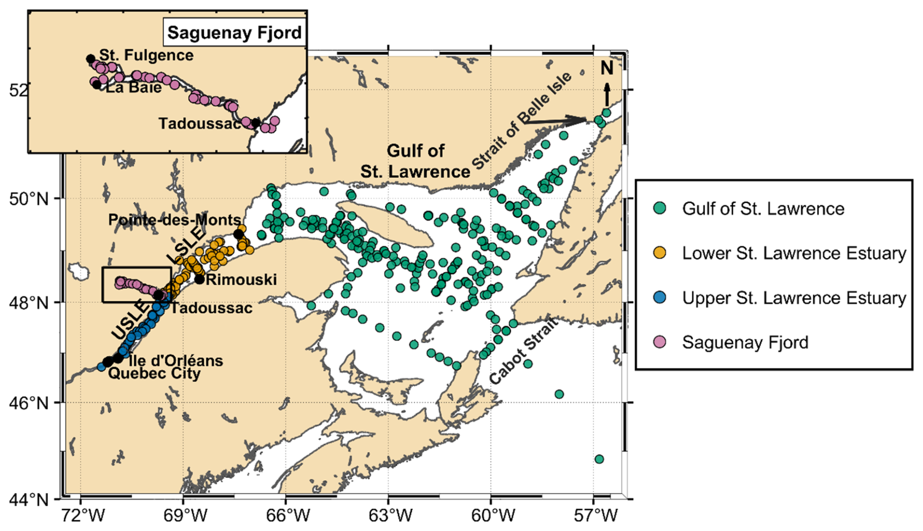
Figure 1 Location of sampling stations in the St. Lawrence system (2003–2023). Points are colour-coded according to the four regions defined and used throughout the manuscript: Gulf of St. Lawrence (GSL; bluish green), Lower St. Lawrence Estuary (LSLE; orange), Upper St. Lawrence Estuary (USLE; blue), and Saguenay Fjord (SF; reddish purple). The black rectangle on the main map marks the Saguenay area; the inset at upper left enlarges the fjord near Tadoussac. Key place names (e.g., Strait of Belle Isle, Cabot Strait, Tadoussac, Île d'Orléans, Québec City, Rimouski, Pointe-des-Monts) are shown for orientation. Coastlines are from the GSHHS fine-resolution shoreline (via M-Map).

Whereas numerous open-ocean data products, with the most notable being GLODAP (Lauvset et al., 2024), have enabled transformative research on large-scale biogeochemical cycles, comparable coastal data products remain scarce and regionally fragmented. The Coastal Ocean Data Analysis Product in North America (CODAP-NA; Jiang et al., 2021) addressed this gap for the North American continental shelf and the Gulf of Mexico, providing a publicly available, quality-controlled synthesis of carbonate-system, oxygen, and nutrient data. It, however, notably omits Canadian coastal regions, such as the Canadian Arctic, Hudson Bay, as well as the Estuary and Gulf of St. Lawrence.

On the Canadian Atlantic margin, the Atlantic Zone Monitoring Program (AZMP; implemented in 1998 by Fisheries and Oceans Canada) provides yearly reports of hydrographic and biogeochemical observations in support of ecosystem and fisheries management. Since 2014, AZMP has included the measurement of at least two carbonate-system parameters as part of these surveys (Galbraith et al., 2025a; Gibb et al., 2023). More recently, the Canadian Atlantic Shelf Temperature-Salinity (CASTS) dataset (Coyne et al., 2026) compiled over 850 000 individual temperature and salinity profiles collected since 1873, providing an open-access, baseline for physical conditions in the northwest Atlantic and eastern Arctic.

Whereas these initiatives have significantly advanced the availability of physical and biogeochemical observations for Atlantic Canada, a regionally integrated, multi-parameter dataset that combines these measurements with additional tracers, organic parameters, and stable isotope data for the EGSL has not been previously assembled. Much of the data collected during dedicated academic and collaborative research cruises, including joint sampling conducted aboard the 2022 AZMP mission, has remained isolated across institutions. The data product presented here is designed to complement, not replace, existing national monitoring programs by providing a harmonized, quality-controlled synthesis of biogeochemical data taken over a 20-year (2003–2023) period in the ESGL as well as the Saguenay Fjord. It consolidates hydrography variables, carbonate-system parameters, dissolved oxygen, nutrient, dissolved organic carbon, stable isotope, and transient tracer data into a single, publicly accessible framework. Although much of the presented data have been exploited in previous publications, until now only a small fraction of it has undergone rigorous, consistent quality control (QC), or been archived in a public repository. Table 1 lists references corresponding to previously archived components of individual cruise datasets, rather than all studies that have used or interpreted these data. As was done in CODAP-NA (Jiang et al., 2021), we applied primary QC procedures while omitting secondary QC methods such as crossover analysis that compares deep-water measurements across cruises to identify systematic biases (Lauvset and Tanhua, 2015; Tanhua et al., 2010). Crossover analysis was not applied here as it is unsuitable in the absence of consistent deep-water (>1500 m) reference samples across the region. By complementing existing efforts such as AZMP, CASTS, GLODAP, and CODAP-NA, the Gulf of St. Lawrence and Estuary Dataset (GOSLED) provides a robust observational foundation for future research on deoxygenation, acidification, and ecosystem change in one of Earth's largest estuarine systems.

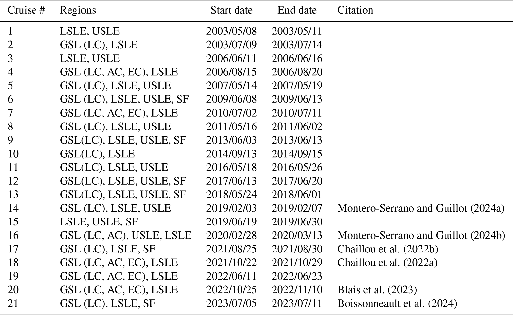
Table 1 The list of cruises included in this data product. Regions are identified as follows: Gulf of St. Lawrence (GSL), Lower St. Lawrence Estuary (LSLE), Upper St. Lawrence Estuary (USLE), and Saguenay Fjord (SF). The channels sampled within the Gulf of St. Lawrence are noted: Laurentian Channel (LC), Anticosti Channel (AC), and Esquiman Channel (EC). Most of the sampled stations in the LSLE are located along the LC, hence the lack of detailed identification. Start and End dates of individual cruises are noted in year/month/day. Partial data from individual cruises that have been previously archived are listed in the “Citation” column.

2 The Estuary and Gulf of St. Lawrence and the Saguenay Fjord

The Gulf (GSL) and St. Lawrence Estuary (SLE) form the downstream connection between the Great Lakes and North Atlantic Ocean through the St. Lawrence River. Draining an area of approximately 1.32×10⁶ km², the St. Lawrence River delivers and average freshwater discharge of 11 900 m³ s⁻¹, making it the second largest in North America, only second to that of the Mississippi. The SLE extends roughly 400 km downstream from the landward front of the salt-water intrusion at the eastern tip of the Île d'Orléans (10–15 km east of Québec City) and stretches 400 km seaward to Pointe-des-Monts where it widens into the GSL. It is conventionally divided into the Upper SLE (USLE) and Lower SLE (LSLE; see Fig. S1 in the Supplement for regional definitions). Extending from the Île d'Orléans to Tadoussac near the mouth of the Saguenay Fjord, the USLE is characterized by a narrow width (2 to 24 km), shallow depths (<30 m), and weak stratification, though it exhibits strong lateral salinity gradients. In contrast, the LSLE, extends from Tadoussac to Pointe-des-Monts and is substantially wider (30–50 km) and deeper (<340 m), exhibiting a smoother bathymetry and pronounced vertical stratification. It opens into the GSL, a large, semi-enclosed sea, connected to the North Atlantic Ocean through the Cabot Strait to the south and Strait of Belle Isle to the north-east.

The primary bathymetric feature of both the GSL and LSLE is the Laurentian Channel (LC). It forms a deep (), U-shaped submarine valley extending ∼1240 km from the continental shelf break, through Cabot Strait, to the head of the LSLE proximal to Tadoussac. Within the eastern GSL, two smaller channels diverge from the LC: the Anticosti Channel (AC) extends westward north of Anticosti Island, whereas the Esquiman Channel (EC) trends northeastward toward the Strait of Belle Isle (Galbraith et al., 2025b). During the ice-free season, the water column of the GSL and LSLE is characterized by a strong three-layer vertical stratification: (1) a freshened surface layer (0–30 m) flowing seaward, (2) a cold intermediate layer (CIL; 50–150 m; Galbraith, 2006) formed in the GSL during winter and flowing inward towards the LSLE, and (3) a upstream-flowing deep layer (>150 m) originating in the western North Atlantic. Historically, this deep layer inflow has been composed of a mixture of LCW and NACW entering through Cabot Strait. As noted earlier, the composition of this deep layer inflow has changed over the past century in response to the retroflection of the Labrador Current off of the Grand Banks (Jutras et al., 2023a), with the inflow predominantly composed of warm, saline, oxygen-poor NACW in recent years of the time series (Jutras et al., 2023b).

The Saguenay Fjord (SF) connects to the head of the LC in the LSLE at Tadoussac. It forms a 110 km long and 2 km wide tributary fjord with a maximum depth of 275 m and a drainage basin of 78 000 km² (Delaigue et al., 2020). Its bathymetry is defined by three sill-bound basins (250, 170 and 275 m deep), with each sill depth (20, 60, and 115 m) becoming progressively deeper landward thus restricting deep-water renewal. The fjord's surface layer consists of a 6–8 m thick brackish wedge for which the fresh water is supplied primarily by the Saguenay River (∼1200 m³ s⁻¹) into the North Arm of the fjord near St. Fulgence and is supplemented by smaller tributaries such as the à Mars and Ha! Ha! Rivers that flow into the Baie des Ha! Ha! (the south arm) as well as the Éternité and Sainte-Marguerite Rivers that discharge along the main axis of the fjord. Beneath this surface layer, the fjord contains dense marine waters that are renewed episodically by overflows of LSLE CIL water across the outer sill, leading to a strongly stratified water column. Seasonal dynamics in the SF are tightly coupled to the conditions of the SLE, with tidal and river discharge modulating stratification (Delaigue et al., 2020).

3 Data collection

This data product represents a 20-year compilation (2003–2023) of discrete biogeochemical measurements from the SLE, GSL, and the SF. The dataset was assembled from individual cruise datasets, laboratory archives, and spreadsheets contributed by multiple investigators and institutions. The first 17 cruises (2003–2021) were primarily sourced from the personal archives of Alfonso Mucci (McGill University), with complementary additions from Yves Gélinas (Concordia University) and Jean-Éric Tremblay (Université Laval). The 2017, 2018, and 2019 summer cruises were supported by the St. Lawrence ECOsystem Health Research and Observation NETwork (SECO.Net) whereas the winter cruises in 2019 and 2020 were funded through the Odyssée St. Lawrence program under the Réseau Québec Maritime (RQM). The four most recent cruises (2021–2023) were conducted by the CERC.OCEAN Lab at Dalhousie University, the Institut des sciences de la mer de Rimouski (ISMER), and the Maurice Lamontagne Institute (Fisheries and Oceans Canada, Mont-Joli) during the Marine Environmental Observation, the Prediction and Response Network (MEOPAR) and RQM lead Gulf of St. Lawrence Tracer Release Experiment (TReX; see Table 1 for summary of cruises).

The locations sampled across the contributing research cruises provide broad spatial coverage of the St. Lawrence system, extending from near Québec City in the USLE to the continental shelf edge beyond Cabot Strait. The water column of the LC was intensively sampled, with additional coverage of the AC and EC in the GSL and repeated occupations in the SF. Collectively, the cruises span winter through late fall, although the majority of fieldwork occurred in spring and summer because of ice conditions and vessel availability (see Fig. 2). The spatial distribution of the 20-year sampling effort is shown in individual cruise maps in the Supplement (Sect. S2) and can be seen as a collective in Fig. 1.

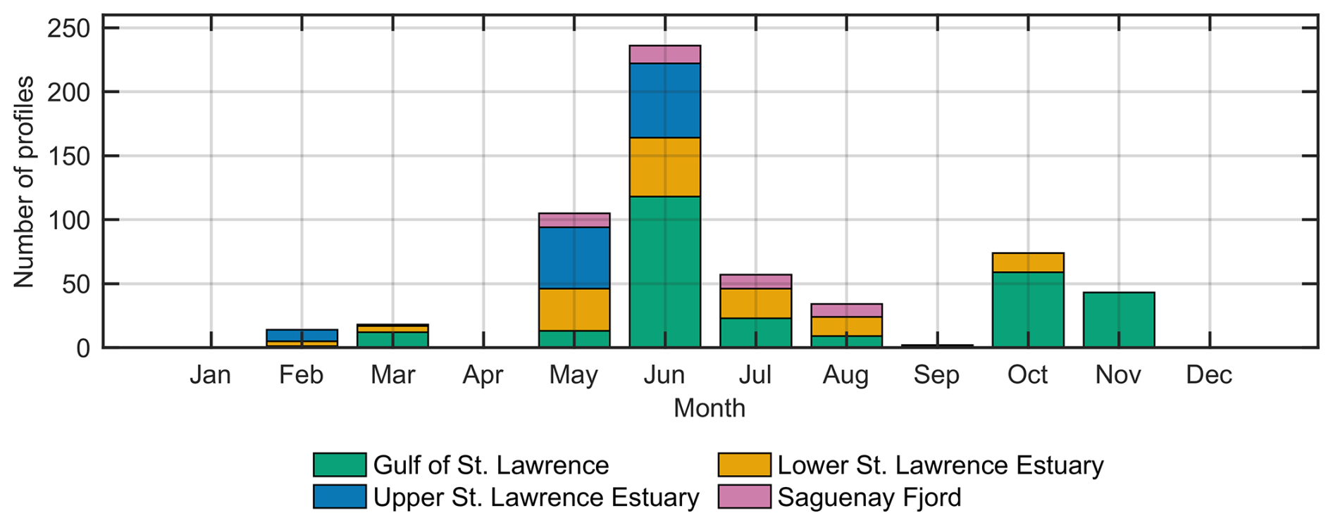
Figure 2 Monthly sampling effort expressed as the number of unique profiles per region. Totals across 2003–2023: All n=584; GSL n=280; LSLE n=142; USLE n=116; SF n=46.

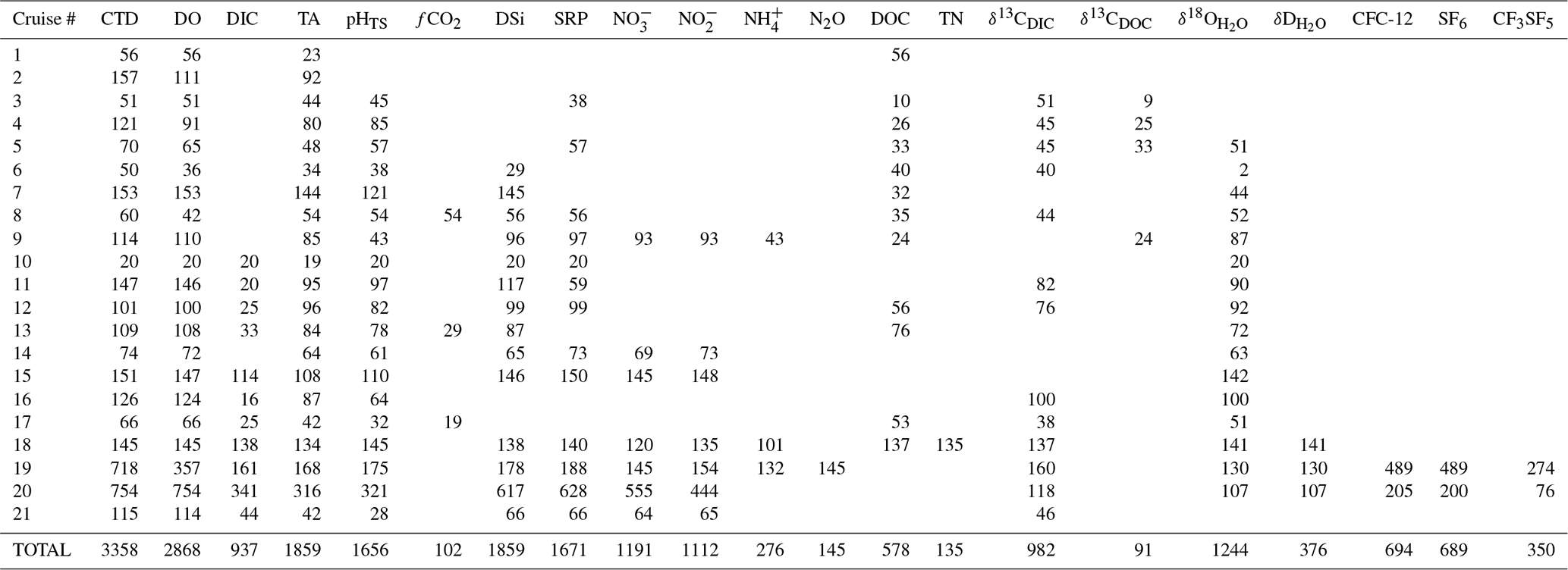
A total of 23 measured parameters is included in the dataset, combining sensor-based CTD measurements with results of discrete water sample analyses (see Table 2). Both manuscript abbreviations and data product variable codes are listed side-by-side in Table 2 to enable direct translation between this paper and the dataset. Sensor-based profiles include pressure, in-situ temperature, practical salinity, CTD-derived dissolved oxygen, and fugacity of CO₂ (fCO₂). Discrete water samples were analyzed for Winkler oxygen (Grasshoff et al., 2009), dissolved inorganic carbon (DIC), total alkalinity (TA), pH on the total proton scale (pH_TS), nutrients (nitrate (${\mathrm{NO}}_{\mathrm{3}}^{-}$), nitrite (${\mathrm{NO}}_{\mathrm{2}}^{-}$), ammonium (${\mathrm{NH}}_{\mathrm{4}}^{+}$), soluble reactive phosphate (SRP), dissolved silicate (DSi)), dissolved organic carbon (DOC), total dissolved nitrogen (TN; dissolved inorganic nitrogen + dissolved organic nitrogen), stable isotopes (δ¹³C_DIC, δ¹³C_DOC, ${\mathit{\delta }}^{\mathrm{18}}{\mathrm{O}}_{{\mathrm{H}}_{\mathrm{2}}\mathrm{O}}$, $\mathit{\delta }{\mathrm{D}}_{{\mathrm{H}}_{\mathrm{2}}\mathrm{O}}$), nitrous oxide (N₂O), transient tracers (CFC-12, SF₆) and the deliberate tracer used in TReX (CF₃SF₅; Stevens et al., 2024). The number of samples taken for each parameter on individual cruises is reported in Table 3. All analytical methods, including instrumentation, detection limits, and cruise-specific procedures, are provided in the Supplement (Sect. S3) and are cross-referenced to each cruise listed in Table 1.

Table 2 Measured parameters included in this data product with their manuscript abbreviations and data product code.

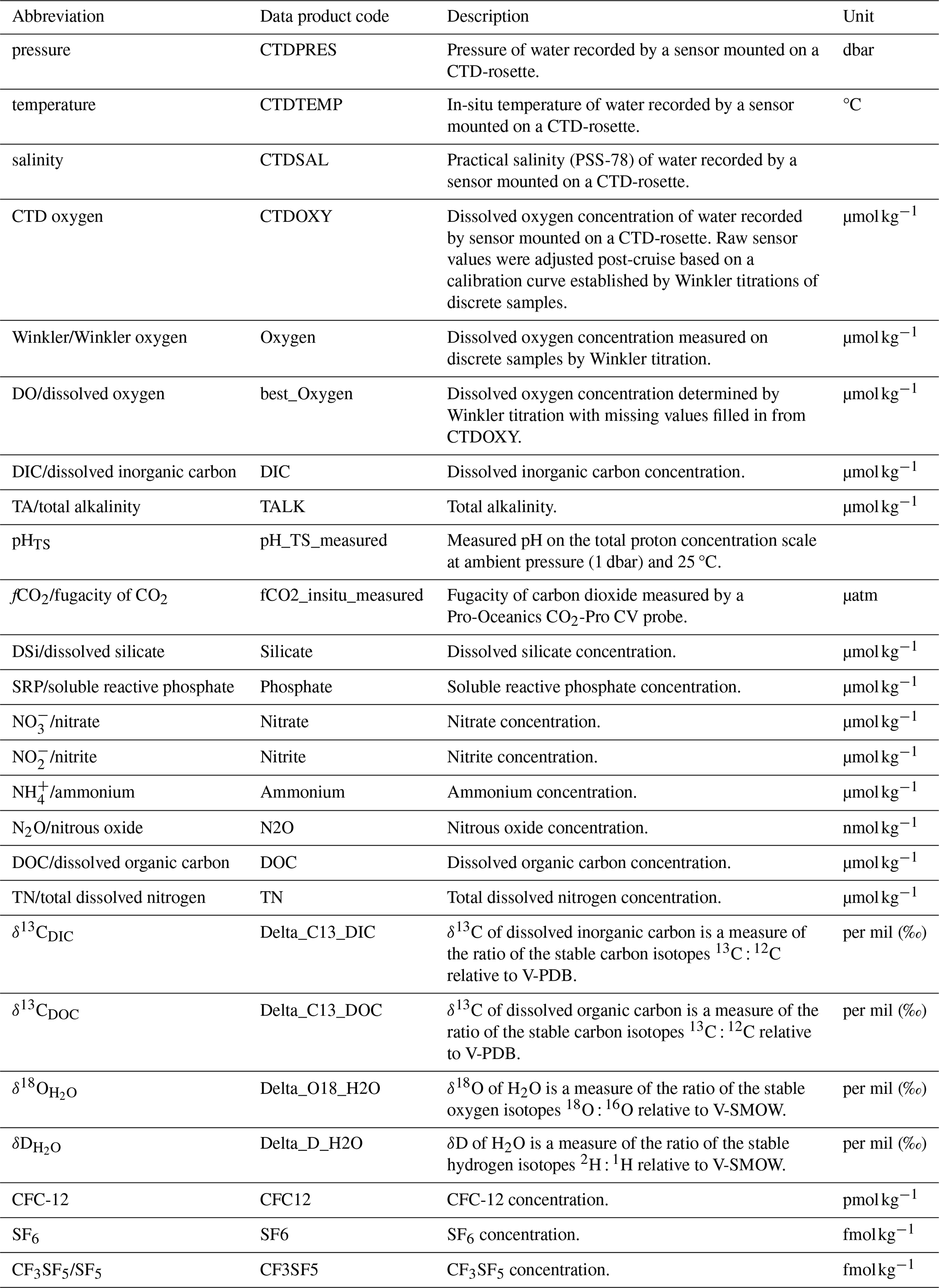
Table 3 Number of valid (flag = 2, non-missing) observations for each measured parameter by cruise. CTD represents concurrent pressure, in-situ temperature, and practical salinity measurements associated to discrete samples; DO includes both CTD oxygen and discrete Winkler measurements (reported as the best_Oxygen variable). Carbonate-system parameters include dissolved inorganic carbon (DIC), total alkalinity (TA), pH on the total proton concentration scale (pH_TS), and fugacity of CO₂ (fCO₂). Nutrients comprise dissolved silicate (DSi), soluble reactive phosphate (SRP), Nitrate (${\mathrm{NO}}_{\mathrm{3}}^{-}$), Nitrite (${\mathrm{NO}}_{\mathrm{2}}^{-}$), and Ammonium (${\mathrm{NH}}_{\mathrm{4}}^{+}$). Additional variables include nitrous oxide (N₂O), dissolved organic carbon (DOC), total dissolved nitrogen (TN), stable isotopes (¹³C_DIC,¹³C_DOC, δ¹⁸O and δD of H₂O), as well as transient (CFC-12, SF₆) and deliberate (CF₃SF₅) tracers. “TOTAL” indicates the cumulative number of quality-controlled samples across all cruises from 2003 to 2023. See Table 1 for cruise region and date information.

Sampling coverage varies both laterally and vertically across the dataset. Depth sampling is not uniform, as stations were sampled at variable and often irregular depth intervals depending on cruise objectives and conditions. Whereas all regions include stations with depth-resolved sampling, some individual stations are limited to surface or near-surface measurements. This variability reflects the diversity of sampling strategies over the 20-year observation period.

4 Methods

4.1 Dataset harmonization and formatting

All original files were parsed and merged into a single, harmonized CSV format with consistent variable naming, column structure, and metadata fields. To ensure compatibility with other global synthesis efforts such as GLODAPv2 (Lauvset et al., 2024) and CODAP-NA (Jiang et al., 2021), all chemical concentrations were standardized to SI units, primarily in moles per kilogram of seawater (e.g. µmol kg⁻¹; see Table 2). Metadata fields, including station coordinates, timestamps, and parameter units were normalized across all entries.

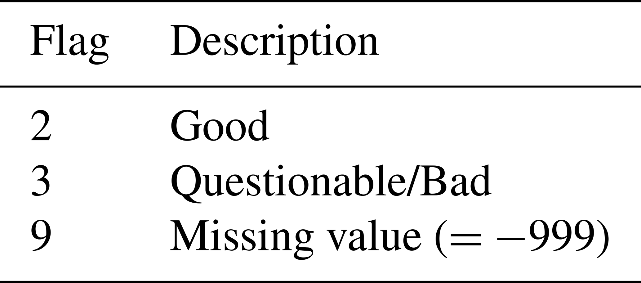
Missing data were encoded using the conventional placeholder value of “−999” and assigned a QC flag value of “9”. All reported values were initially assigned a flag of “2” (good) prior to QC screening. The flagging system used is summarized in Table 4.

Table 4 Summary of QC flags used in this study.

Given the geographic extent of the EGSL as well as the regionally specific hydrography and water column stratification in the various channels, regional identifiers were assigned to each profile to avoid the identification of false outliers. The regional identifiers (Region) were defined as follows: Gulf of St. Lawrence = 1, Lower St. Lawrence Estuary = 2, Upper St. Lawrence Estuary = 3, and Saguenay Fjord = 4. Furthermore, binary identifiers were assigned to indicate if a profile was located within the Laurentian Channel (LC), Anticosti Channel (AC), or Esquiman Channel (EC) (1 = present, 0 = absent). These indicators were assigned manually based on station coordinates and their placement on a map in relation to bathymetry. Stations outside these three main channels were coded as a 0 in each column, whereas some samples lie in multiple or all channels, such as just inside Cabot Strait, where the three channel branches form, were assigned a value of 1 in two or more columns. This structure facilitates regional analysis and provides the framework for the quality control procedures described below.

4.2 Primary quality control framework

In the absence of deep-water observations (>1500 m), a prerequisite for secondary QC techniques such as crossover analysis, the present dataset solely underwent primary QC. This approach follows the standards established in other large-scale syntheses like CARINA (Key et al., 2010; Tanhua et al., 2010), GLODAPv2 (Lauvset et al., 2024), CASTS (Coyne et al., 2026) and, perhaps most relevant to this effort, CODAP-NA (Jiang et al., 2021), with adaptations suited to the stratified and regionally heterogenous nature of the EGSL system.

Primary QC involves identifying and flagging implausible or inconsistent values within individual profiles, among regional clusters, and across property-property relationships. It does not attempt to apply multi-cruise consistency adjustments (e.g. inter-calibrated offsets) that would be inappropriate in dynamic, shallow coastal systems. Instead, we focus on producing a transparent and regionally contextualized dataset for users to build upon.

Given the distinct physical and biogeochemical characteristics of the four major subregions: the GSL, LSLE, USLE, and SF, each profile was assessed in the context of its regional variability. This region-specific approach avoided false flagging of valid data that deviate from global norms but are consistent within the regional oceanography (e.g., freshwater lenses, hypoxic zones, high nutrient layers, or acidified bottom waters).

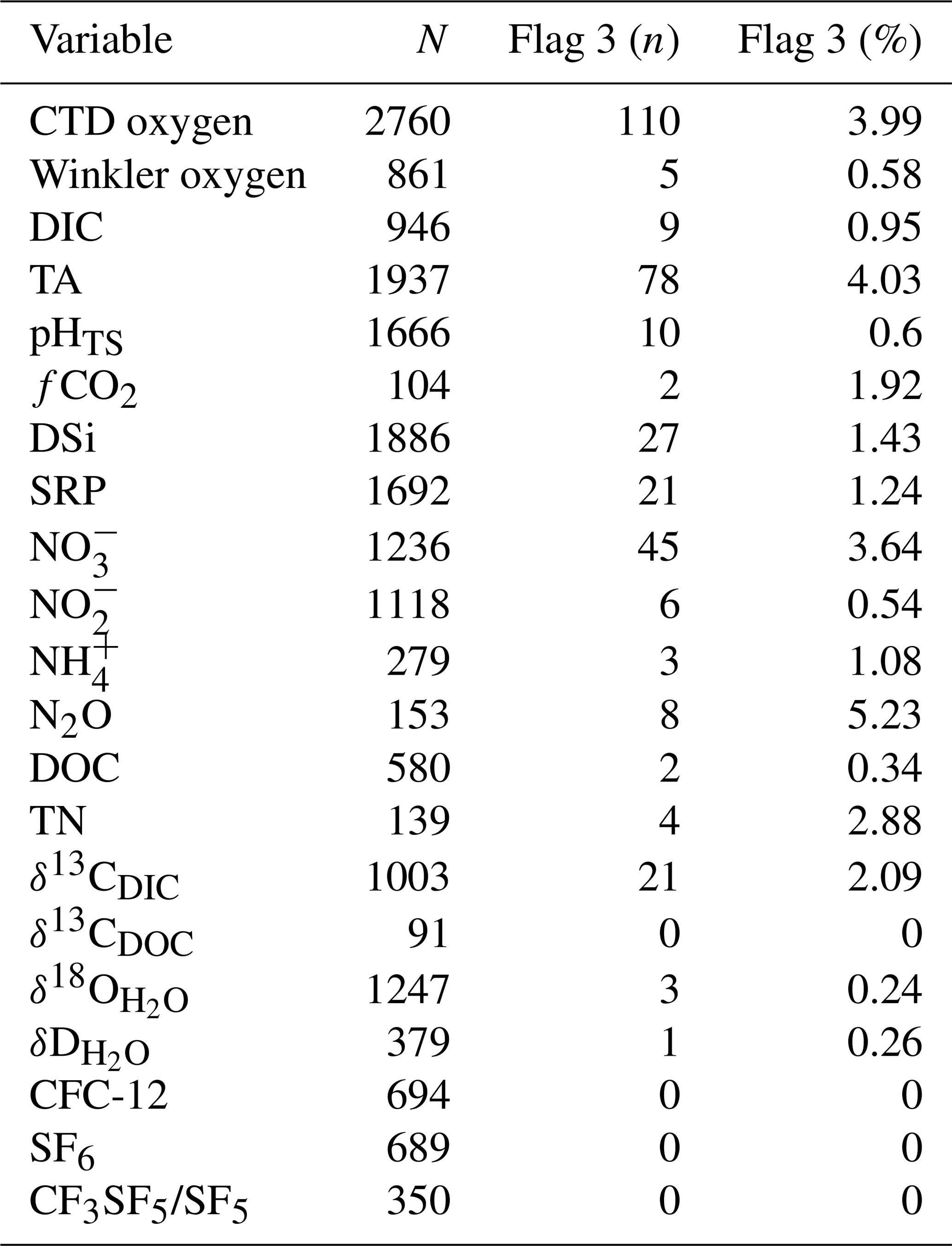
All profiles were visually examined with parameters plotted against pressure (analogous with depth in this case) while overlaying with regionally aggregated profiles derived from the full dataset. Particular attention was paid to shape irregularities (e.g., sawtooth shapes, abrupt trend reversals, etc.) that often reflect bottle misfires, sampling contamination, or sensor drift. Obvious single-point outliers were assigned a QC flag of “3” (questionable) and retained in the dataset with their original values for transparency. To complement these visual diagnostics, automated acceptance criteria were applied to selected property-property relationships within each region. Robust (Huber-weighted) linear fits were generated for key pairs (${\mathrm{NO}}_{\mathrm{3}}^{-}$-AOU, N₂O-AOU, δ¹³C_DOC-DOC, etc., where AOU stands for Apparent Oxygen Utilization ($=[\text{DO}{]}_{\text{sat}}-[\text{DO}{]}_{i-s}$). Fits and ±3σ envelopes, are shown and data falling outside of these thresholds were flagged as questionable (flag =3). This 3σ threshold effectively captures extreme deviations while preserving the natural scatter associated with spatial and seasonal variability. Elemental ratios, such as N:P, were evaluated qualitatively but were not used to assign flags as natural deviations from the Redfield ratios (Redfield et al., 1963) occur frequently in estuarine and coastal waters (Paradis-Hautcoeur et al., 2023). Likewise, internal consistency checks for the carbonate-system were performed but not used to modify flags. Together, these procedures constitute a transparent, regionally-tuned QC framework. The resulting flags and residual diagnostics provide a foundation for secondary evaluations and cross-calibration efforts. The proportion of observations flagged as questionable (flag =3) was low across all parameters, typically below 5 % (see Table 5), with no systematic patterns identified across cruises, regions, or sampling periods.

Table 5 Summary of QC flags across measured parameters. N denotes the number of valid observations (excluding missing values), while n denotes the number of observations flagged as questionable (Flag =3). Percentages represent the proportion of flagged values relative to N for each parameter.

4.3 Dissolved oxygen (CTD oxygen and Winkler)

Dissolved oxygen data in this product originate from two sources: a Sea-Bird Scientific SBE43 CTD-mounted oxygen probe and discrete Winkler oxygen titrations. For all cruises, CTD dissolved oxygen data had undergone post-cruise calibration by the Principal Investigators (PIs) or scientific data managers through regression of matched sensor-Winkler pairs. The resulting cruise-specific fits were then applied to the unmatched CTD oxygen values to correct them to an inferred Winkler-equivalent concentration. These adjusted values were adopted in the present dataset. Subsequent tests confirmed close agreement between sensor and discrete values across the dataset, indicating that this calibration step was consistently implemented. The resulting adjusted CTD oxygen values are the ones reported in the final product.

Following Grégoire et al. (2021), we adopted a threshold of ±10 µmol kg⁻¹ as the acceptable deviation between each sample that have both CTDOXY and paired Winkler measurements (see Fig. 3). If $|\text{CTD oxygen}-\text{Winkler}|>\mathrm{10}$ µmol kg⁻¹, the CTD oxygen value was noted as questionable (flag =3). To provide a single, consistent oxygen field for analyses, a composite variable “best_Oxygen” was generated using the following hierarchy:

$$\begin{array}{rl}& \text{Winkler}(\text{flag}=\mathrm{2})>\text{CTD oxygen}(\text{flag}=\mathrm{2})\\ & >\text{Winkler}(\text{flag}=\mathrm{3})>\text{CTD oxygen}(\text{flag}=\mathrm{3}).\end{array}$$

The first available value in this sequence was adopted, and its original flag was propagated to the composite column. This ensures that the highest-quality measurement (usually Winkler titration) is retained where available while maintaining transparency for users.

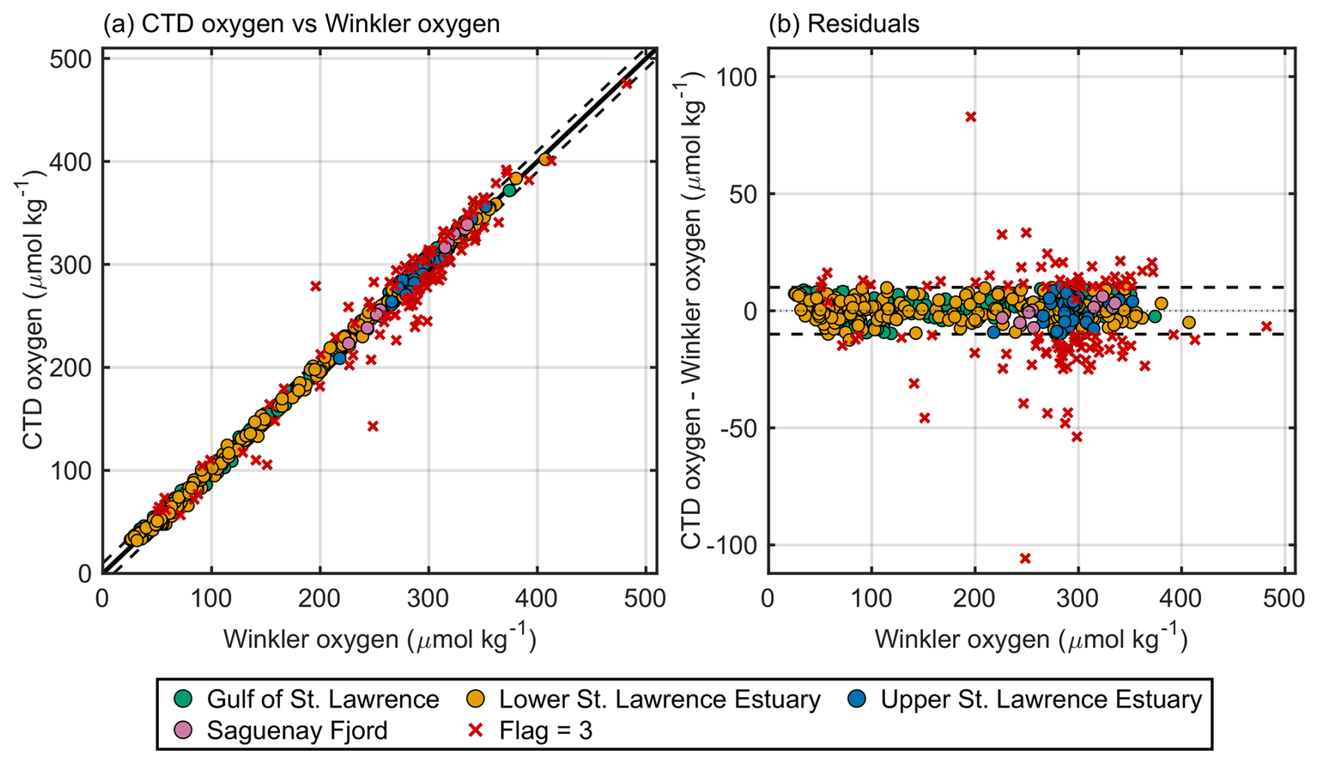
Figure 3 Comparison of CTD-probe dissolved oxygen measurements with results of discrete Winkler titrations across the St. Lawrence system (2003–2023). (a) CTD oxygen vs. Winkler oxygen; the solid line is 1:1 and the dashed lines denote an acceptance band of ±10 µmol kg⁻¹. Points are coloured by region. (b) Residuals, defined as CTD Oxygen – Winkler oxygen, versus Winkler; dashed lines again indicate ±10 µmol kg⁻¹. Filled symbols represent data flagged as good (Flag =2); red “×” indicate measurements flagged as questionable (Flag =3) and are shown for transparency but not used in performance evaluation. Units are µmol kg⁻¹ throughout.

The QC'd oxygen field (best_Oxygen in the data product; see Table 2) was subsequently used to calculate the AOU, as it serves as a diagnostic tracer to evaluate the internal consistency of other redox-sensitive parameters. AOU provides a quantitative measure of remineralization and is thus compared with other variables (i.e., nutrients, nitrous oxide etc.) in later QC steps and is included in the final data product.

4.4 Carbonate chemistry (pH_TS, TA, DIC, fCO₂)

First, TA was plotted against the practical salinity and the DSi concentrations for each region to identify obvious analytical or sampling outliers. Clear outliers were assigned flag =3 (questionable). Evaluations presented in this section are intended to illustrate data behaviour and patterns within the dataset and provide completeness of the description of the data. Comparisons between measured and calculated carbonate-system parameters are therefore used to highlight systematic offsets and visualize variability across regions and are not used as a basis for flag assignment. Carbonate-system calculations were performed in MATLAB version R2024a with the CO2SYSv3 package (Lewis and Wallace, 1998; Sharp et al., 2020). As prescribed by Dickson et al. (2007), the following constants were selected for these calculations: carbonic acid dissociation constants of Lueker et al. (2000), bisulfate dissociation constant of Dickson (1990), hydrofluoric acid dissociation constant of Perez and Fraga (1987), and total borate concentration of Lee et al. (2010).

It is important to note that the choice of equilibrium constants can significantly influence calculated carbonate-system parameters under low-salinity (<20) or cold (<8 °C) conditions. Several studies have shown that the constants of Cai and Wang (1998) return improved agreement of fCO₂ and pH_TS values in low-salinity and estuarine waters (Delaigue et al., 2020; Dinauer and Mucci, 2017; Minor and Brinkley, 2022). Likewise, the formulations of Waters et al. (2014) have also been recommended for brackish waters. In colder coastal regions, the Lueker et al. (2000) constants may underestimate fCO₂ and overestimate pH_TS in surface waters (Sulpis et al., 2020). Despite these considerations, the Lueker et al. (2000) constants were retained to maintain consistency with published best practices (Dickson et al., 2007) as well as GLODAP and CODAP-NA. The objective of this manuscript is to provide a consistent, quality-controlled dataset. Hence, a systematic assessment of constant selection and its impact on carbonate system calculations, while worthwhile, is beyond the manuscript's scope. A full propagation of uncertainty would require resolving multiple coupled equilibria involving numerous acid-base systems and equilibrium constants (Carter et al., 2024). This has been partially addressed in previous publications in this region (Delaigue et al., 2020; Dinauer and Mucci, 2017, 2018; Fradette, 2025; Mucci et al., 2011; Mucci and Jutras, 2026) and should be further considered in future use of this dataset.

Residuals between measured and calculated parameters were evaluated against arbitrary envelopes (±25 µmol kg⁻¹ for TA and DIC, ±0.15 for pH_TS, and ±60 µatm for fCO₂). Residuals exceeding these limits were qualitatively investigated but not used to assign flags, given the difficulty of attributing them unambiguously to a single parameter in coastal and estuarine waters. This approach allows visualization of how carbonate-system variables behave across regions while avoiding over-interpretation of residual structure in a setting where natural variability and methodological diversity are prevalent. Each parameter evaluation is described in the subsections below.

4.4.1 pH_TS

pH_TS data showed the largest variability relative to calculated values of all carbonate-system parameters. In the GSL and LSLE, residuals (pH_TS – pH(TA,DIC)) were mostly within ±0.15 unit, though persistent positive residuals were noted, meaning that measured pH_TS was significantly higher than pH_TS calculated from TA and DIC (pH_TADIC in the data product). Notably, in the USLE and SF, residuals increased substantially, sometimes exceeding +0.6 pH unit (see Fig. 4).

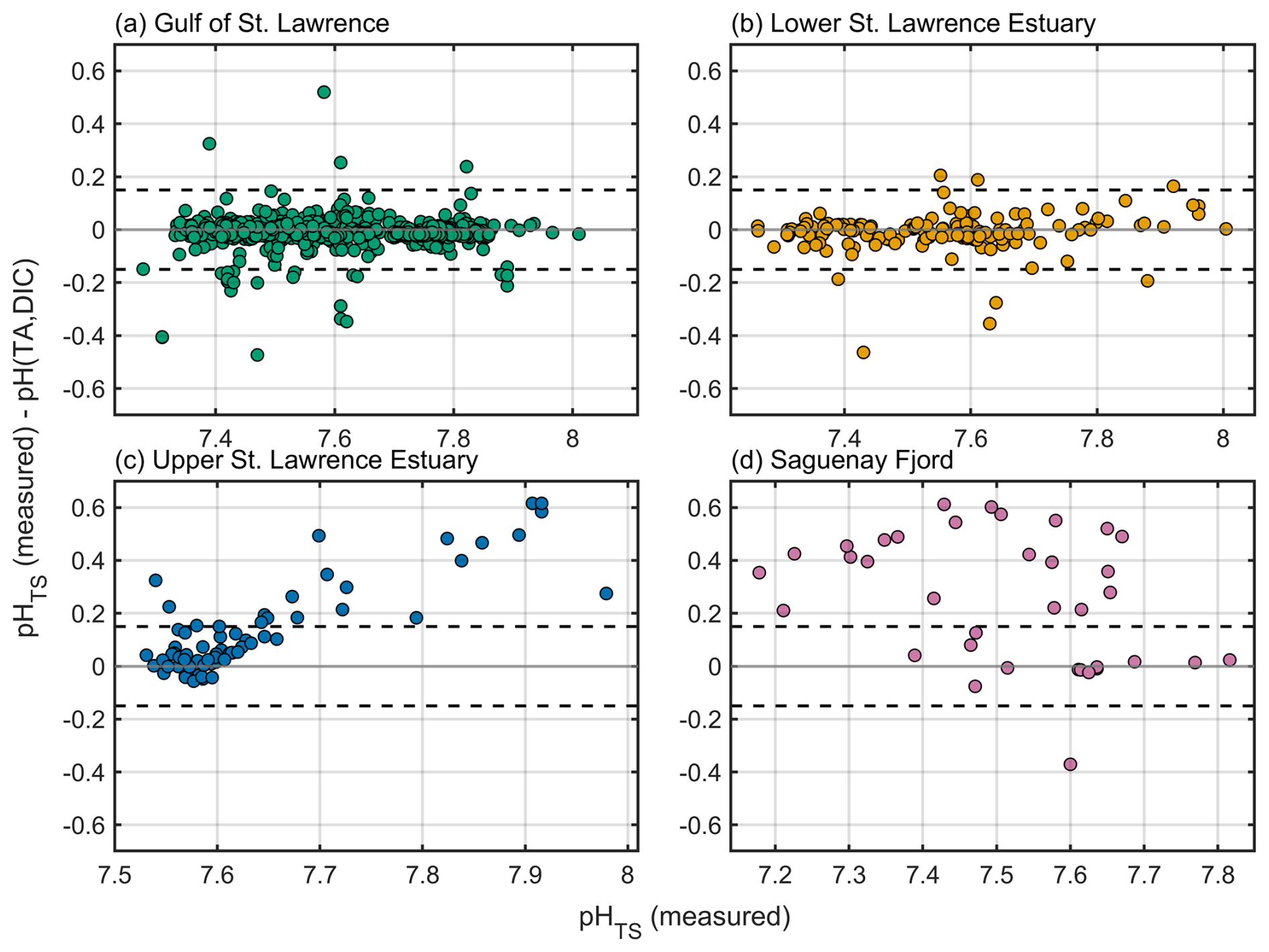
Figure 4 Behaviour of pH_TS relative to calculated values by region. Residuals are computed as pH_TS (measured) – pH(TA,DIC) and plotted versus pH_TS (measured) for (a) Gulf of St. Lawrence, (b) Lower St. Lawrence Estuary, (c) Upper St. Lawrence Estuary, and (d) Saguenay Fjord. Only samples with QC flag =2 are shown. The grey line denotes zero residual, and the darker, dashed lines border the ±0.15 pH_TS band. Shared y-axes allow direct comparison among regions; the scatter about zero reflects combined measurement and calculation uncertainty, whereas any coherent offsets highlight potential region-specific patterns.

The deviations likely reflect methodological and compositional sources of uncertainty. At reduced ionic strength, the optical properties of indicator dyes, temperature-sensitivity of equilibrium constants, and incomplete standardization to the total proton scale can contribute to deviations (Carter et al., 2024; Patsavas et al., 2015). The indicator dye itself adds a small but measurable alkalinity component, that if unaccounted for, produces an overestimation of pH_TS (Carter et al., 2024; Dickson et al., 2007; Fradette, 2025). As previously mentioned, at reduced salinity, differences in the choice of carbonic acid dissociation constants (Cai and Wang, 1998; Lueker et al., 2000; Waters et al., 2014) together with uncharacterized organic alkalinity, can further amplify offsets between measured and calculated variables in humic-rich environments such as in the SF (Delaigue et al., 2020) and USLE (Qudsi et al., 2024). Since carbonate-system parameters are interdependent, even small pH_TS errors can lead to large offsets in calculated DIC and TA. Consequently, the consistent direction of the residuals likely reflects a combination of analytical uncertainties and unresolved organic alkalinity contributions.

4.4.2 Total alkalinity

TA measurements exhibit agreement with calculated values across the GSL and LSLE (Fig. 5). In these regions, TA calculated from measured pH_TS and DIC (TALK_pHDIC in the data product) generally aligned well with observed TA, with most residuals falling within ±25 µmol kg⁻¹. Measured values, however, tended to exceed calculated TA (TA > TA(pH,DIC)), indicating systematic offsets between measured and calculated variables arising from a combination of factors, including uncertainties in pH_TS measurements, the choice of equilibrium constants, the presence of organic alkalinity (Carter et al., 2024). Similar features have been documented in productive, freshwater-influenced systems where weak organic acids and bases are not represented in standard CO₂-system calculations (Cai and Wang, 1998; Kerr et al., 2023; Kim and Lee, 2009; Martín Hernández-Ayon et al., 2007; Patsavas et al., 2015; Song et al., 2020), including the surface waters of the SF (Delaigue et al., 2020).

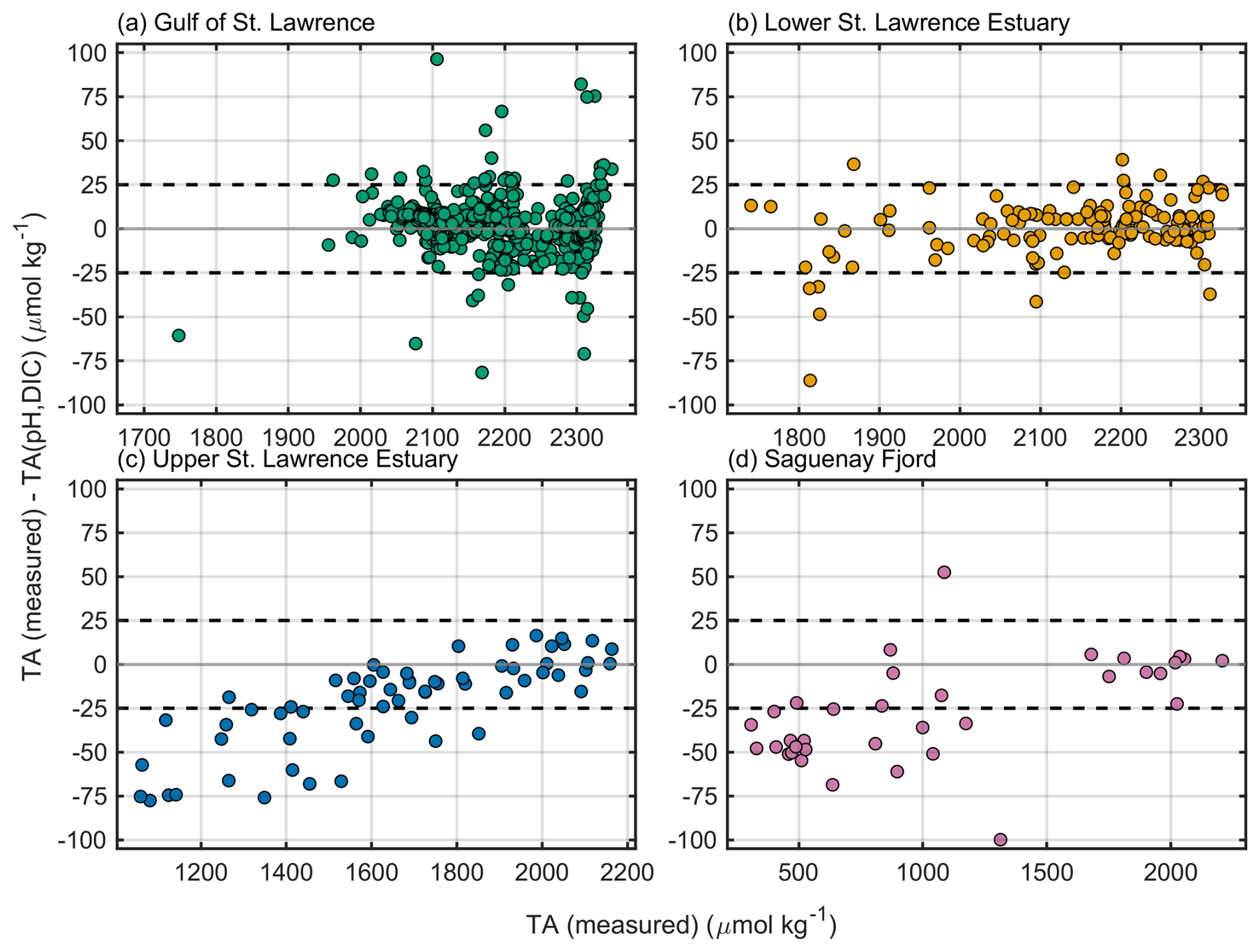
Figure 5 Behaviour of TA relative to calculated values by region. Panels show the residual TA (measured) – TA(pH,DIC) versus TA (measured) for (a) Gulf of St. Lawrence (GSL), (b) Lower St. Lawrence Estuary (LSLE), (c) Upper St. Lawrence Estuary (USLE) and (d) Saguenay Fjord (SF). TA(pH,DIC) is the carbonate-system TA recalculated from paired pH_TS and DIC measurements. Only measurements with quality Flag =2 are plotted. The dashed lines border a ±25 µmol kg⁻¹ band around zero; the grey line marks zero residual. Shared y-axes allow direct comparison among regions; the scatter about zero reflects combined measurement and calculation uncertainty, whereas any coherent offsets highlight potential region-specific patterns.

In contrast, residuals in the USLE and SF were predominantly negative (TA < TA(pH, DIC)) and increased in magnitude toward lower salinities. These offsets likely reflect both reduced buffer capacity of low-salinity waters and increasing uncertainty of thermodynamics constants below a salinity ≈20, where the seawater dissociation constants for carbonic and boric acids along with the boron-salinity relationship are more poorly constrained (Carter et al., 2024; Patsavas et al., 2015). As reported by Delaigue et al. (2020), organic alkalinity in the Saguenay River can be significantly negative ($-\mathrm{33}\pm \mathrm{3}$ µmol kg⁻¹), whereas smaller, positive contributions are observed in the EGSL, particularly at low salinity.

As previously stated, since pH_TS was used to calculate both TA and DIC, even seemingly small uncertainties in pH_TS can propagate into relatively large offsets in derived TA. The spread observed here therefore likely reflects a combination of analytical uncertainties in pH_TS, measured-method differences (Sharp and Byrne, 2020) and unidentified alkalinity contributions (e.g. organic alkalinity), rather than a single defined cause (Fradette, 2025).

4.4.3 Dissolved inorganic carbon

DIC measurements were generally in agreement with calculated values (DIC_pHTA in the data product) in the GSL and LSLE (see Fig. 6). Most residuals fell within ±25 µmol kg⁻¹ indicating agreement across these regions. A few negative residuals (DIC < DIC(pH,TA)) were observed and likely reflect the combined influence of pH_TS uncertainty and unidentified alkalinity contributions. As discussed in the previous sections, small offsets in pH_TS can propagate into significant DIC residuals.

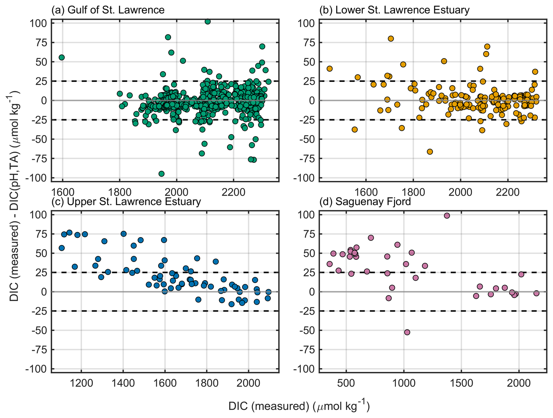
Figure 6 Behaviour of DIC relative to calculated values by region. Residuals are computed as DIC (measured) – DIC(pH,TA) and plotted versus DIC (measured) for (a) Gulf of St. Lawrence, (b) Lower St. Lawrence Estuary, (c) Upper St. Lawrence Estuary and (d) Saguenay Fjord. Only samples with QC flag =2 are shown. The grey line marks zero residual and the darker, dashed lines border the ±25 µmol kg⁻¹ band. Shared y-axes allow direct comparison among regions; the scatter about zero reflects combined measurement and calculation uncertainty, whereas any coherent offsets highlight potential region-specific patterns.

Residuals increased in magnitude at lower salinities in the USLE and SF, consistent with the combined effects of reduced buffering, uncharacterized acid-base species, and uncertainties in the carbonate-system constants at salinities below 20. These deviations mirror the regional trends described for TA and pH_TS and underscore the interconnected nature of these biases: the same low-salinity samples showing elevated ΔpH_TS typically correspond to larger ΔDIC and ΔTA values (Patsavas et al., 2015).

4.4.4 Fugacity of CO₂

Measured fCO₂ showed overall agreement with values calculated from other carbonate-system parameter pairs (Fig. 7). Across all regions, most residuals (fCO₂ (measured) – fCO₂ (calculated)) fell within ±60 µatm. No clear systematic bias pattern was observed among the three parameter combinations tested (pH_TS-DIC, TA-DIC, pH_TS-TA; or within the data product, fCO2_pHDIC, fCO2_TADIC, and fCO2_pHTA respectively), although scatter increased significantly in the USLE and SF, consistent with the lower precision of pH_TS and TA under freshwater influence in DOC-rich and poorly buffered regions.

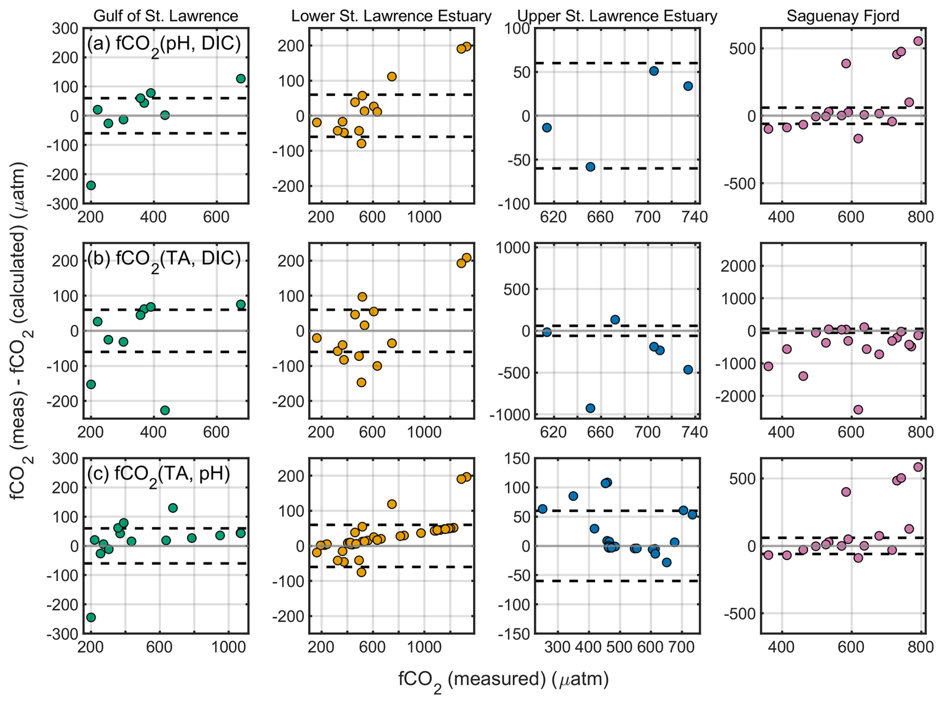
Figure 7 Behaviour of fCO₂ relative to calculated values by region. Residuals are defined as fCO₂ (measured)-fCO₂ (calculated) and are plotted against fCO₂ (measured) (µatm). Columns show regions (Gulf of St. Lawrence, Lower St. Lawrence Estuary, Upper St. Lawrence Estuary, Saguenay Fjord); rows show the variable pairs used to calculate fCO₂ (calculated): (a) pH_DIC; (b) TA_DIC; (c) TA_pH. Only samples with quality flag =2 are included (2003–2023). The grey line marks a zero residual; darker, dashed lines denote the ±60 µatm acceptance band. Positive values indicate measured fCO₂ higher than the value reconstructed from the given pair. Regional x axis limits reflect the local fCO₂ ranges.

Interestingly, the TA-DIC pair produced the least consistent fCO₂ values, differing from the general pattern of pH_TS-related uncertainty observed in the other carbonate diagnostics. This divergence likely reflects excess or unidentified components of alkalinity as previously discussed. In these low-salinity regimes, deviations likely reflect propagated uncertainty from the companion variables and the omission of organic alkalinity in calculations, rather than measurement error of fCO₂ itself. Given the limited number of direct fCO₂ measurements, fCO₂ data were retained without adjustment and are interpreted primarily as a comparative reference across carbonate-system variables.

4.4.5 Carbonate-system summary

Overall, the carbonate-system parameter visualisations presented above illustrate that apparent residuals among TA, DIC, pH_TS, and fCO₂ largely reflect the compounded uncertainties described in Carter et al. (2024). Specifically, where differences in methodology (particularly in pH_TS), choice of equilibrium constants, and potential uncharacterized alkalinity components likely led to deviations, particularly in low salinity, DOC-rich, poorly buffered waters (i.e. USLE and SF). Although large residuals were observed for pH_TS, the TA-DIC pair produced the greatest deviations when evaluated through calculated fCO₂, an outcome that underscores the complicated thermodynamic and methodological uncertainties in these regions. This counterintuitive result underscores that no single parameter pair provides universally reliable closure across the full salinity range.

Consequently, these comparisons are therefore used to describe dataset behaviour and variability, rather than as a criterion for flag adjustment or formal evaluation. Future work should prioritize refining thermodynamic constraints and internal consistency approaches for estuarine and low-salinity waters, where deviations from seawater composition challenge the robustness of current carbonate-system parameter calculations.

4.5 Nutrients

Nutrient data were evaluated through individual profile inspection and regional property-property analyses following the primary-QC framework described above. Each dissolved nutrient (nitrate, nitrite, ammonium, soluble reactive phosphate (SRP), and silicate (DSi)) was assessed in the context of its vertical distribution, regional norms, and expected stoichiometric relationships. Clear analytical outliers were assigned a flag =3 (questionable) and retained for transparency.

For nitrate, concentration profiles displayed strong and coherent vertical structure across most regions, generally increasing with depth in stratified water columns (see Fig. 14 in Sect. 5). Property–property plots with SRP revealed Redfield-like slopes in the GSL and LSLE (Fig. 8), whereas samples from the USLE displayed local departures with a weak or nonlinear relationship at low SRP concentrations (<1 µmol kg⁻¹). Deep-water nitrate plateaus were observed around 25 µmol kg⁻¹ in the LSLE, and near 10 µmol kg⁻¹ in the SF. A consistent positive relationship between nitrate and AOU was evident across most subregions (apart from the USLE; Fig. 8), confirming coupling between remineralization and oxygen consumption.

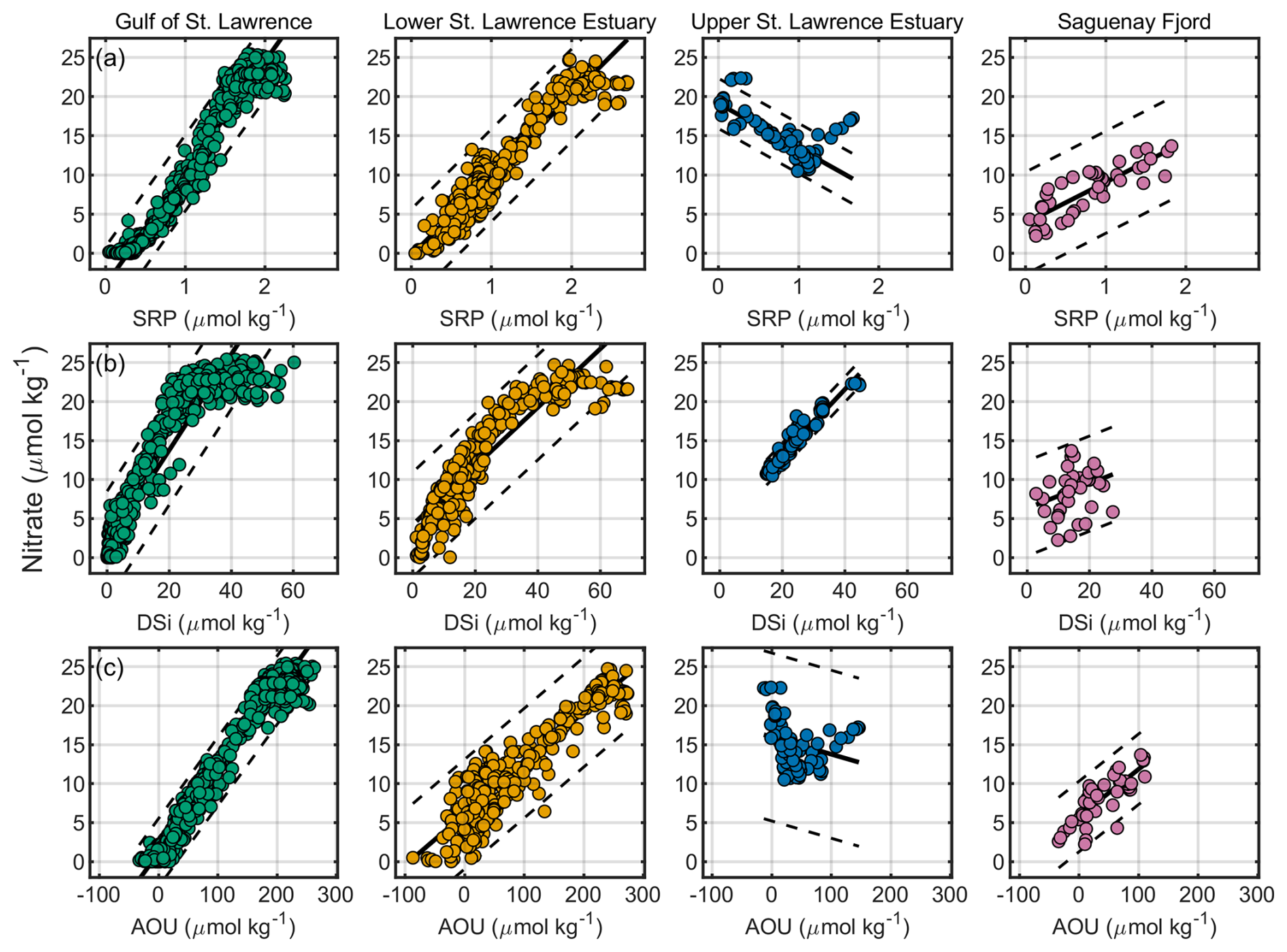
Figure 8 Property–property relationships by region. Columns show the Gulf of St. Lawrence, Lower St. Lawrence Estuary, Upper St. Lawrence Estuary, and Saguenay Fjord. Rows are (a) Nitrate vs. soluble reactive phosphate (SRP), (b) Nitrate vs. dissolved silicate (DSi), and (c) Nitrate vs. apparent oxygen utilization (AOU). Only samples with primary QC flag =2 are plotted (filled circles; colors by region). Black lines are robust linear fits computed separately for each region; dashed lines border the ±3σ envelope. Properties on both axes are in µmol kg⁻¹. Bands are shown to illustrate internal consistency; Nitrate vs. SRP is treated as a secondary diagnostic, with potential outliers corroborated against Nitrate-AOU before any flag changes. Overall, relationships are internally consistent across regions.

Automated regional regressions were applied for nitrate against SRP, DSi, and AOU, using ±3σ acceptance envelopes (see Sect. 4.2). Points outside these ranges were visually reviewed, and only clear analytical outliers were flagged. Deviations from the classical Redfield ratio (Redfield et al., 1963; N:P $\approx \mathrm{16}:\mathrm{1}$) were not used as a flagging criterion, as such variability is expected in estuarine and shelf systems influenced by differential regeneration, denitrification, and sedimentary fluxes.

Nitrite concentrations were generally low, with distinct subsurface maxima occurring at AOU values of ∼50 and 200 µmol kg⁻¹ (Fig. 9). These features were most pronounced in the stratified GSL and LSLE, consistent with active nitrification or partial denitrification zones (Crowe et al., 2012). Depth profiles show narrow peaks (see Fig. 14 in Sect. 5), consistent with localized redox transition zones (Wang et al., 2003).

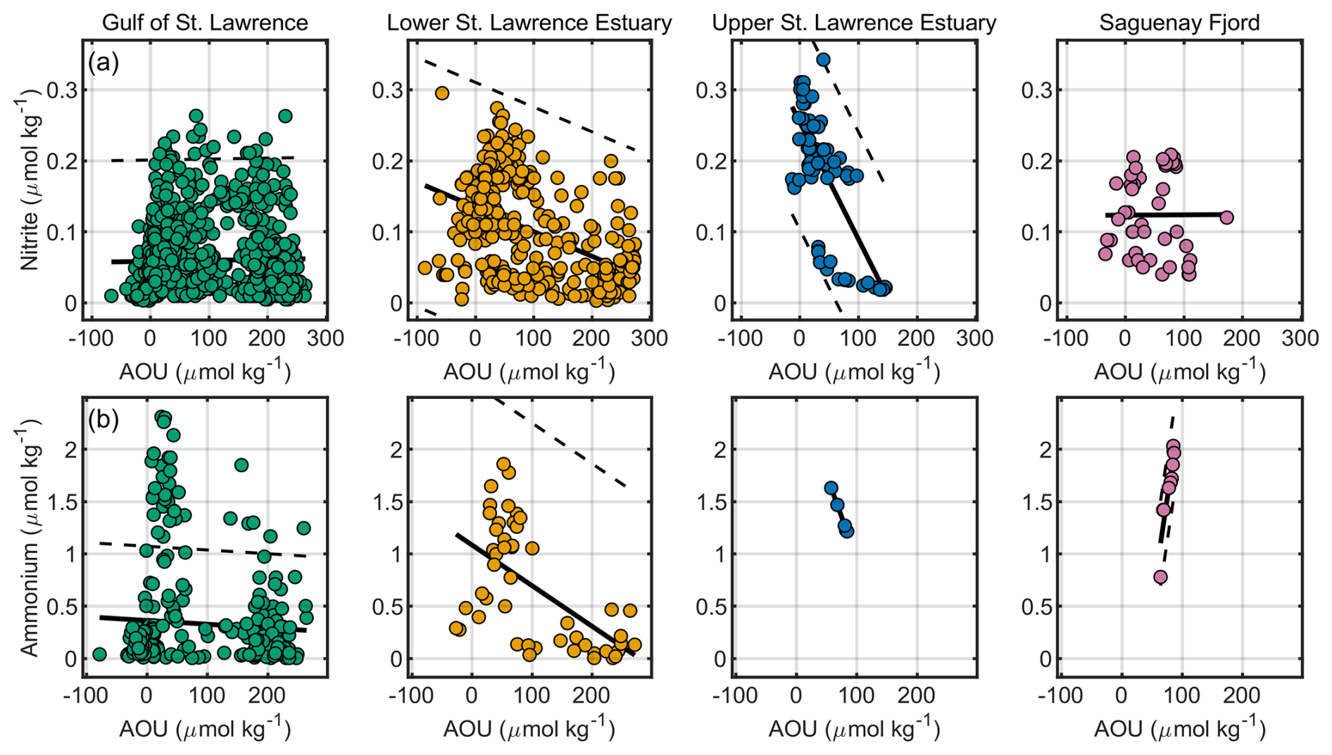
Figure 9 Property–property relationships by region. Columns show the Gulf of St. Lawrence, Lower St. Lawrence Estuary, Upper St. Lawrence Estuary, and Saguenay Fjord. Rows are (a) Nitrite vs. AOU and (b) Ammonium vs. AOU. Only samples with primary QC flag =2 are plotted (filled circles; colors by region). Black lines are robust linear fits computed separately for each region where sufficient data are available; dashed lines border the ±3σ envelope. All properties are reported in µmol kg⁻¹.

Ammonium profiles exhibited subsurface peaks that co-occurred with those of nitrite but with greater amplitude (Fig. 9). Concentrations were elevated below the photic zone, near the sediment–water interface, and in high-AOU (low-oxygen) waters, reflecting remineralization/degradation of organic matter under oxygen-limited conditions. These maxima were particularly pronounced in the GSL.

SRP concentrations displayed a strong positive correlation with AOU across all regions, increasing with depth as remineralization progressed. This trend was robust throughout the GSL, SLE, and SF, though slightly weaker in the USLE and SF. The observed profiles reflect the combined effects of remineralization and benthic release of SRP from sediments (Pascal et al., 2025), processes that can occur well before fully reducing conditions are reached (Katsev et al., 2007; Lefort, 2012; Sundby et al., 1986, 1992).

DSi showed a similar relationship, increasing with AOU and depth. Concentrations were highest in the LSLE and GSL deep layers (up to 60–70 µmol kg¹), and remained elevated near the seafloor in the SF, consistent with benthic regeneration in stratified, organic-rich environments.

4.6 Nitrous oxide, dissolved organic carbon, and total dissolved nitrogen

Profiles of N₂O, DOC and TN were examined for outliers and regionally-consistent trends following the primary-QC framework. Outlier detection combined visual inspection of vertical profiles (see Figs. 14 and 15 in Sect. 5) for all three parameters with additional property–property comparisons against AOU for N₂O. Implausible values were assigned flag =3 (questionable) and retained for transparency.

N₂O measurements were available only in the GSL and LSLE (Fig. 10), as no samples were collected in the USLE and SF. Across the investigated regions, N₂O concentrations increased systematically with AOU, peaking just below the surface mixed layer in waters with AOU >100 µmol kg¹. Regional regressions of N₂O versus AOU showed strong positive slopes within ±3σ envelopes, consistent with nitrification–denitrification coupling under suboxic conditions (Pascal et al., 2025). The relationship was most pronounced in the LSLE, where clusters of elevated-AOU and N₂O concentrations corresponded to oxygen-deficient waters of the LC.

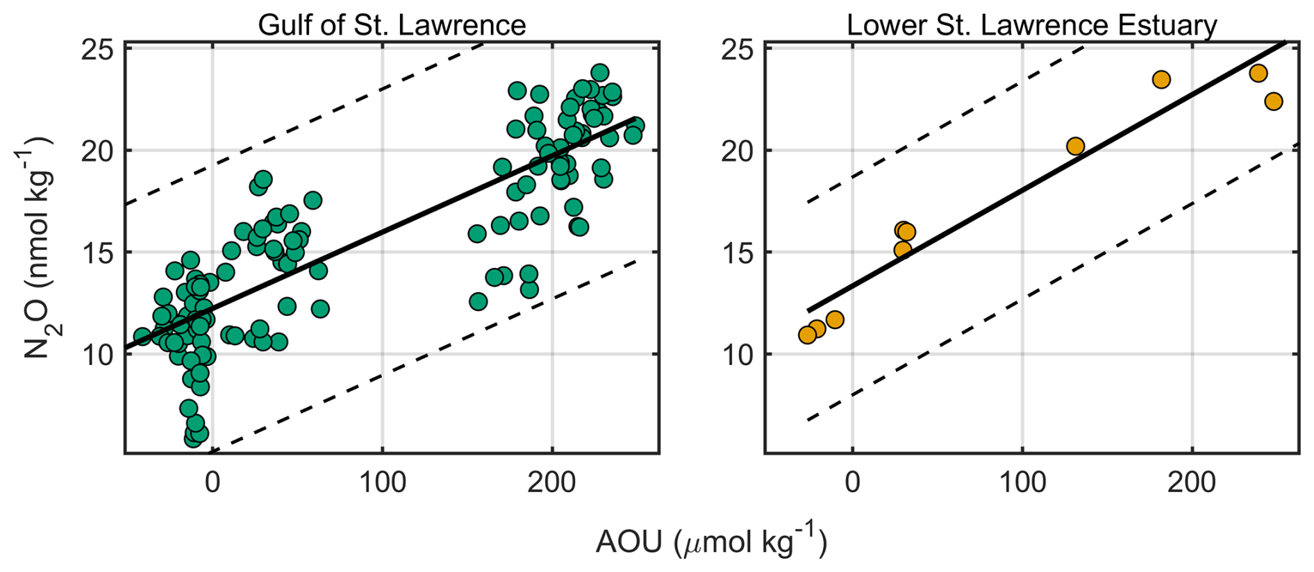
Figure 10 Nitrous oxide (N₂O) vs. AOU. Panels show the Gulf of St. Lawrence (left) and Lower St. Lawrence Estuary (right), the two regions with sufficient paired observations. Only measurements with a primary quality flag =2 are plotted (filled circles). Black lines indicate robust linear fits; dashed lines delimit the ±3σ residual envelope estimated from the median absolute deviation.

DOC displayed a classical profile structure, with elevated surface concentrations that decayed exponentially with depth. DOC typically stabilized near 50 µmol kg⁻¹ below ∼150 m, consistent with the transition from reactive to refractory carbon pools (LaBrie et al., 2020). Surface values were slightly higher in the USLE and SF, reflecting greater relative terrestrial and freshwater inputs and/or its release from suboxic sediments (Hélie and Hillaire-Marcel, 2006; Lévesque et al., 2023; Qudsi et al., 2024). No systematic inter-regional offsets were identified.

TN profiles exhibited an inverse pattern to DOC, with concentrations lowest at the surface and increasing with depth to a stable mean of ∼25 µmol kg⁻¹ below ∼150 m. The deep-water enrichment of TN reflects the accumulation of inorganic nitrogen species regenerated during organic matter remineralization. When considered jointly, the DOC and TN distributions highlight the vertical decoupling of organic and inorganic nitrogen pools within the St. Lawrence system.

4.7 Stable isotope measurements

All stable isotope profiles were visually screened for outliers and evaluated for internal consistency using regional regressions and expected isotopic–property relationships (δ¹³C_DIC-AOU, δ¹³C_DOC-DOC, and ${\mathit{\delta }}^{\mathrm{18}}{\mathrm{O}}_{{\mathrm{H}}_{\mathrm{2}}\mathrm{O}}$–$\mathit{\delta }{\mathrm{D}}_{{\mathrm{H}}_{\mathrm{2}}\mathrm{O}}$; see Fig. 11). Linear fits and ±3σ envelopes were used to identify implausible values, following the general QC framework described in Sect. 4.2.

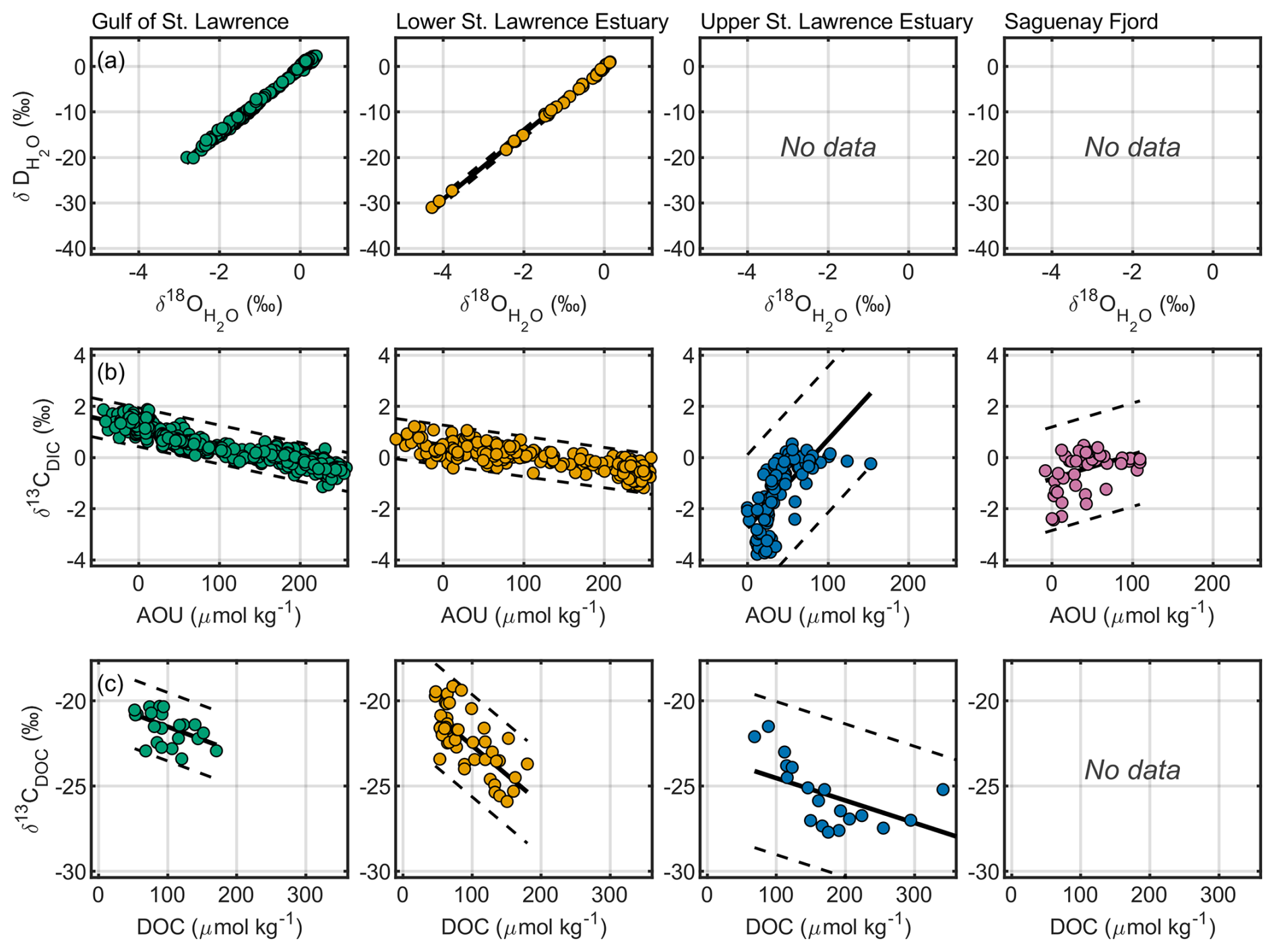
Figure 11 Isotopic relationships by region. Rows show (a) ${\mathit{\delta }}^{\mathrm{18}}{\mathrm{O}}_{{\mathrm{H}}_{\mathrm{2}}\mathrm{O}}$ versus $\mathit{\delta }{\mathrm{D}}_{{\mathrm{H}}_{\mathrm{2}}\mathrm{O}}$, (b) δ¹³C_DIC versus apparent oxygen utilization (AOU), and (c) δ¹³C_DOC versus dissolved organic carbon (DOC). Only data with a primary quality flag =2 for the measured stable isotopes are shown. Black lines denote robust linear fits, with dashed lines delineating the ±3σ envelope based on the median absolute deviation.

δ¹³C_DIC values in the GSL and LSLE exhibited vertically coherent profiles consistent with marine carbonate-system dynamics. Surface waters showed typical marine signatures of +1 ‰ to +2 ‰ (relative to Vienna Pee Dee Belemnite (VPDB)), decreasing systematically with increasing AOU and depth to approximately −1 ‰ at 250–300 m (see Fig. 16 in Sect. 5). These gradients reflect progressive release of isotopically light inorganic carbon during organic matter remineralization and mixing with Atlantic-derived DIC at depth. The δ¹³C_DIC–AOU slopes agree with model-derived remineralization rates for the LC reported by Nesbitt et al. (2025).

In the USLE, δ¹³C_DIC values were more variable and generally depleted (−4‰ to 0‰; see Fig. 16 in Sect. 5), consistent with freshwater inputs and in-situ respiration of organic carbon. The SF data, although limited, showed similarly low and weakly stratified values (−2 ‰ to −1 ‰), reflecting a restricted deep-water renewal and a stronger terrigenous influence (Qudsi et al., 2024).

δ¹³C_DOC values (−22 ‰ to −27 ‰) were depleted relative to those of DIC, consistent with organic matter of mixed terrestrial and planktonic origin. The strongest depletions occurred in the USLE and SF, where terrestrial organic carbon inputs dominate (Barber et al., 2017; Tremblay and Gagné, 2009)

The water isotopes, ${\mathit{\delta }}^{\mathrm{18}}{\mathrm{O}}_{{\mathrm{H}}_{\mathrm{2}}\mathrm{O}}$ and $\mathit{\delta }{\mathrm{D}}_{{\mathrm{H}}_{\mathrm{2}}\mathrm{O}}$, displayed linear covariance (slope =7.23, R²=0.998 in the GSL; slope =7.23 and R²=0.999 in the LSLE), consistent with the global meteoric water line (Craig, 1961). Values increased with depth and salinity, reflecting conservative mixing between isotopically light riverine water (δ¹⁸O $\approx -\mathrm{15}$ ‰ to −20 ‰ VSMOW; δD $\approx -\mathrm{100}$ ‰ to −140 ‰) and heavier Atlantic inflows (δ¹⁸O ≈0 ‰; δD ≈0 ‰). Profiles in the GSL and LSLE followed this two-endmember structure closely, confirming internal consistency between isotope and hydrographic data (Dinauer and Mucci, 2018).

Overall, isotopic parameters exhibited high internal consistency and physically coherent mixing relationships. Variations among regions primarily reflect salinity-driven endmember mixing and redox-linked fractionation during organic matter remineralization, rather than analytical offsets. Future QC efforts should continue to test isotopic stability in estuarine gradients, where freshwater–marine transitions and the complexity of the organic carbon cycle (multiple sources, photosynthesis and respiration) may challenge internal consistency approaches.

4.8 Deliberate and Transient Tracers

Measurements of three gaseous tracers (CFC-12, SF₆, and CF₃SF₅) were included in the later years of the dataset, particularly during the 2022–2023 Gulf of St. Lawrence Tracer Release Experiment (TReX). Of these, CF₃SF₅ was a deliberate tracer, released and tracked to directly investigate the dispersion and ventilation pathways of the deep inflow in the LC (Stevens et al., 2024). The other two compounds, CFC-12 and SF₆, are well-established transient tracers that provide context for water mass age and transit times, and are used for cross-validation of ventilation estimates based on the dispersion of the deliberate tracer (Gerke et al., 2026; Stevens et al., 2024). All three tracers were measured simultaneously.

QC focused on ensuring internal consistency between cruises. Profile distributions were visually inspected to confirm agreement with neighbouring casts. Data from the two 2022 cruises (TReX2 (Cruise #19) and DFO AZMP Fall 2022 (Cruise #20)) were compared in T-S space and against expected atmospheric concentrations, displaying elevated variability in the Cruise #20 data. To correct for this systematic offset, measurements from Cruise #20 were uniformly scaled by −20 % for CFC-12, −14 % for SF₆, and −17 % for CF₃SF₅, bringing them into agreement with Cruise #19 observations and with conceivable atmospheric equilibrium saturation in surface waters. Thus, these parameters were rigorously quality-controlled at the analytical stage by the laboratory personnel performing the gas extractions and analyses. Tracer profiles were visually inspected during compilation to confirm consistency with adjacent depth structure and to ensure that regional patterns matched known distributions. No additional profile-level outliers were flagged.

5 Data records

The full 20-year biogeochemical dataset for the Estuary and Gulf of St. Lawrence as well as the Saguenay Fjord is publicly archived through the Canadian Integrated Ocean Observing System – St. Lawrence Global Observatory (CIOOS-SLGO) under the DOI: https://doi.org/10.26071/d6f3fdfc-788d-48ff (Nesbitt et al., 2026). The dataset is provided as a comma-separated value (CSV) file in long-format, where each row represents a unique sample depth within a given profile. All metadata fields (e.g., station coordinates, cruise identifier, regional assignments) are included alongside the measured parameters, and column headers follow naming conventions compatible with GLODAPv2 and CODAP-NA standards.

The file includes 23 unique measured parameters together with sensor metadata and identifiers. All chemical concentrations are reported in SI units, primarily per kilogram of seawater (e.g., µmol kg⁻¹) and each variable is accompanied by a QC flag. Regional identifiers are provided to distinguish between the Gulf of St. Lawrence, Lower and Upper Estuary, and the Saguenay Fjord. Additional binary indicators specify whether a profile is located within the Laurentian, Anticosti, or Esquiman Channels.

The following figures (Figs. 12–17) illustrate the vertical and regional distribution of all parameters included in the final post-QC dataset. Each panel presents depth profiles separated by subregion and coloured accordingly, providing a visual summary of the spatial coverage, vertical extent, and data density for each parameter group: including hydrographic variables, carbonate chemistry, nutrients, redox-linked tracers, stable isotopes, and gaseous tracers. “No data” indicate where measurements were unavailable or did not meet minimum QC thresholds. Together, these figures summarize the integrated outcome of the QC and harmonization process, demonstrating the breadth and internal consistency of GOSLED.

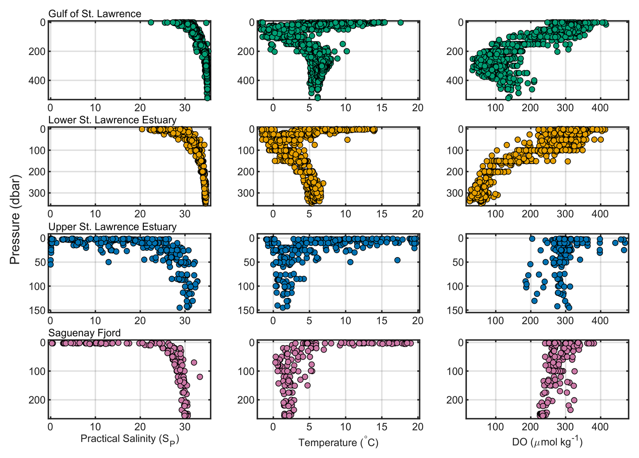
Figure 12 Depth profiles of practical salinity, temperature, and DO (best_Oxygen) by region. Only flag =2 values are plotted. Note that the depth range varies across regions.

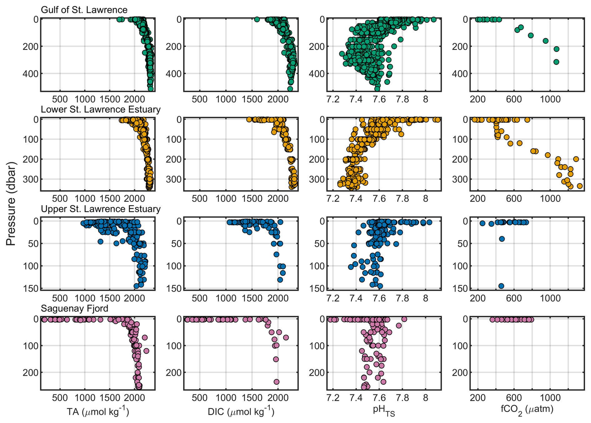
Figure 13 Depth profiles of TA, DIC, pH_TS, and fCO₂ by region. Only flag =2 values are included. Note that the depth range varies across regions.

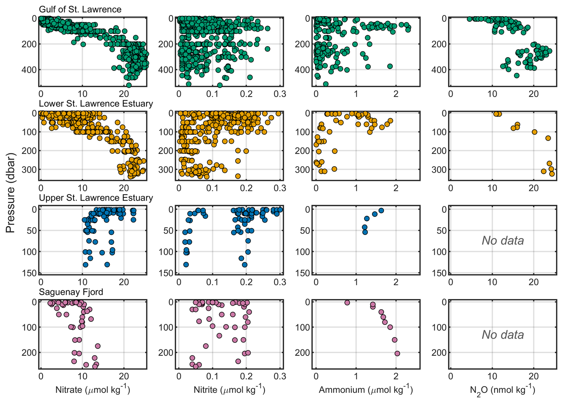
Figure 14 Depth profiles of dissolved nitrate, nitrite, ammonium, and N₂O by region. Only flag =2 values are shown; tiles without data are labelled “No data”. Note that the depth range varies across regions.

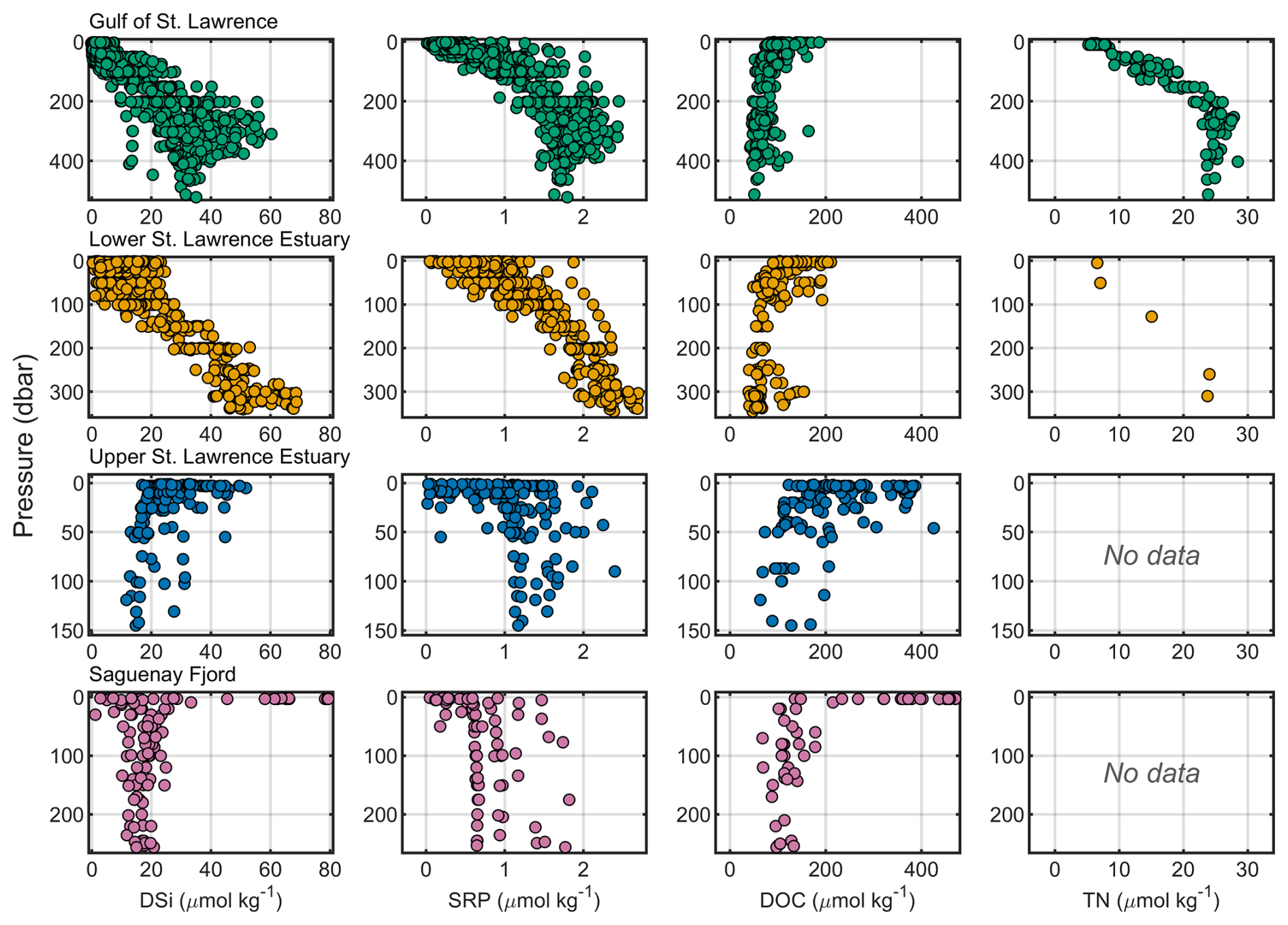
Figure 15 Depth profiles of dissolved silicate (DSi), soluble reactive phosphate (SRP), DOC, and TN by region. Only flag =2 values are shown; tiles without data are labelled “No data”. Note that the depth range varies across regions.

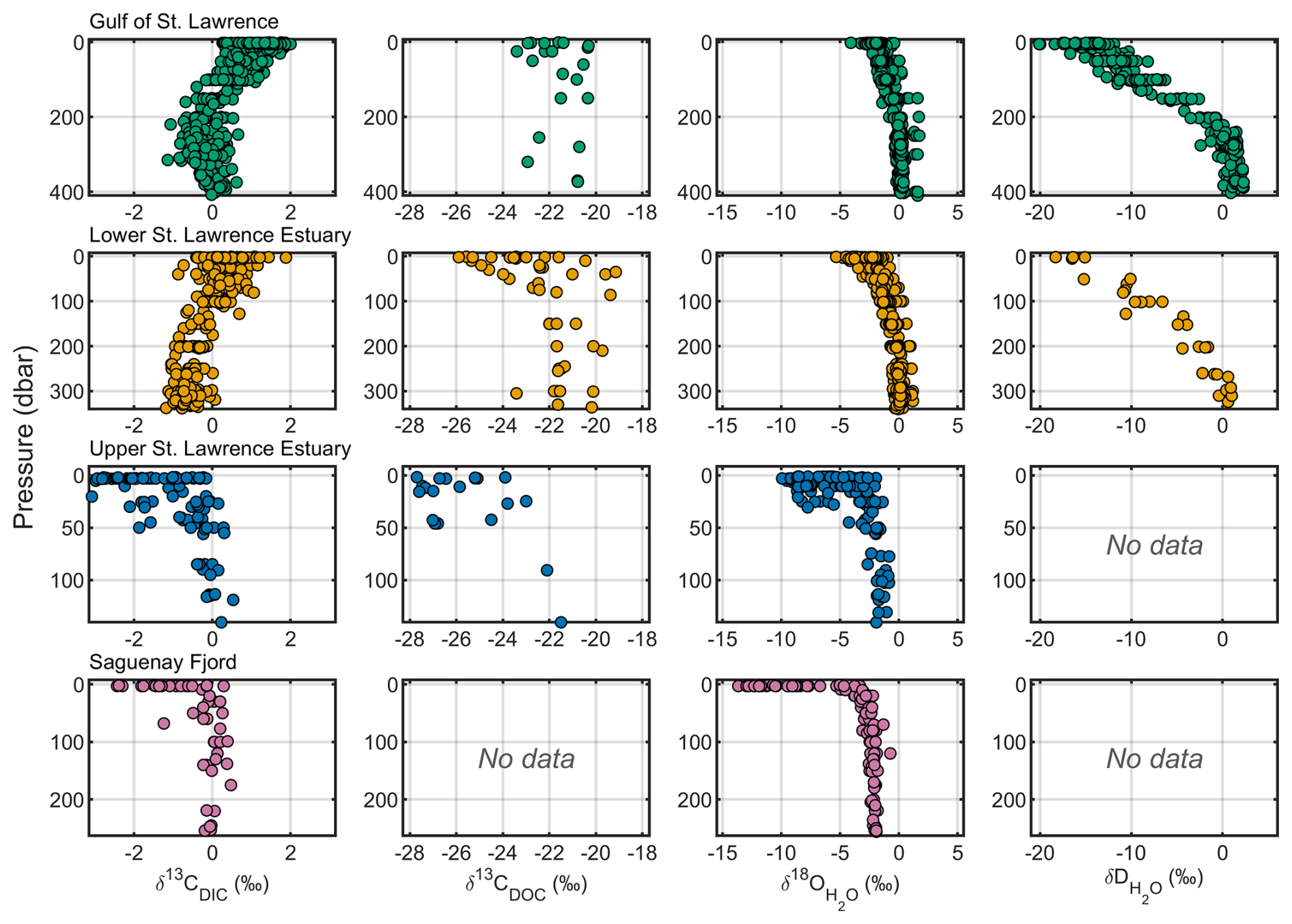
Figure 16 Depth profiles of δ¹³C_DIC, δ¹³C_DOC, ${\mathit{\delta }}^{\mathrm{18}}{\mathrm{O}}_{{\mathrm{H}}_{\mathrm{2}}\mathrm{O}}$, and $\mathit{\delta }{\mathrm{D}}_{{\mathrm{H}}_{\mathrm{2}}\mathrm{O}}$ by region. Only flag =2 values are shown; tiles without data are labelled “No data”. Note that the depth range varies across regions.

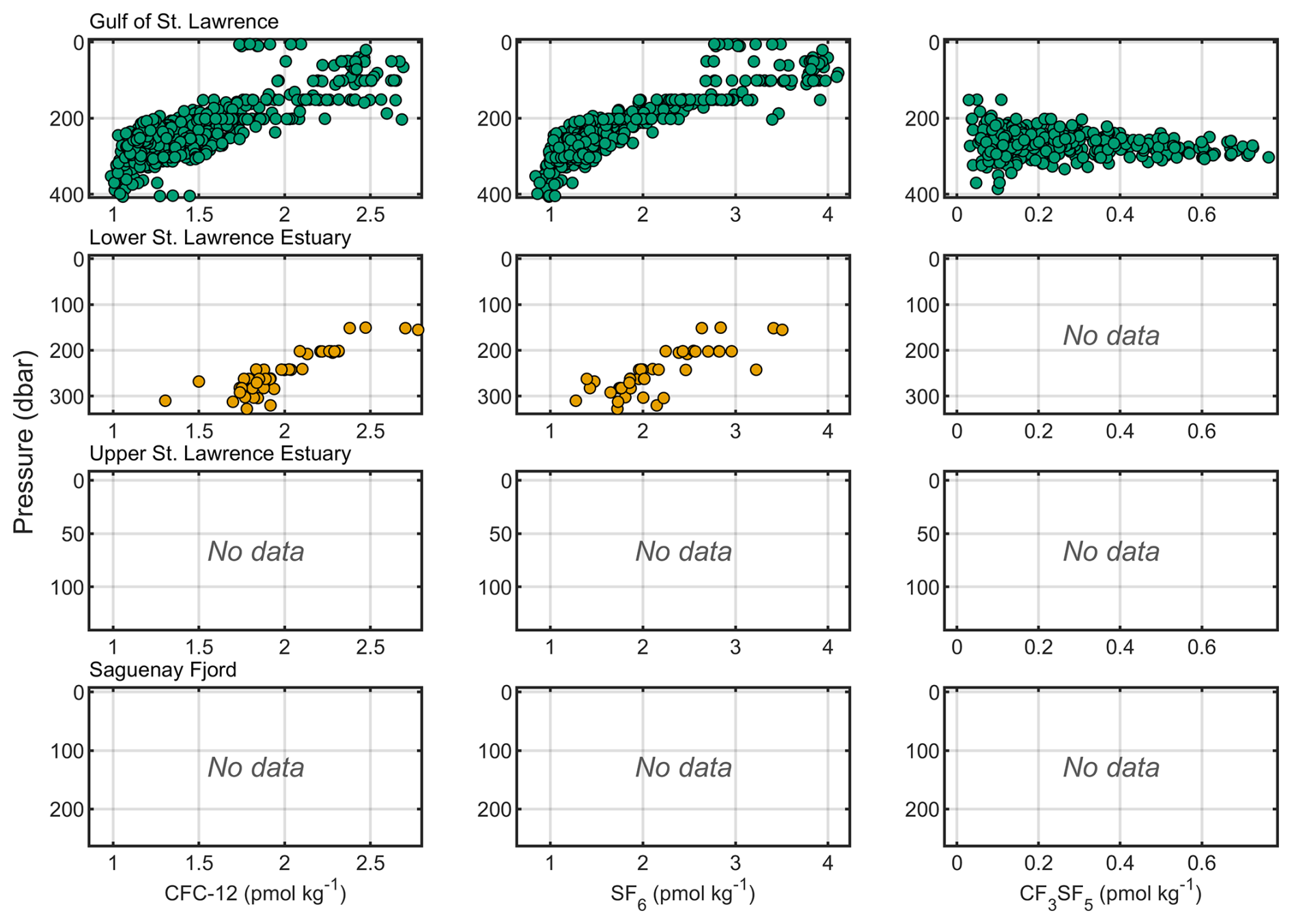
Figure 17 Depth profiles of CFC-12, SF₆, and CF₃SF₅ by region Only flag =2 values are shown; tiles without data are labelled “No data”. Note that the depth range varies across regions.

6 Discussion and validation

This section synthesizes the outcomes of the quality control procedures described in Sect. 4 and evaluates the dataset in terms of parameter behaviour, agreement among measurements, and known limitations. The dataset underwent primary QC, following established protocols used in synthesis products such as GLODAPv2 (Lauvset et al., 2024) and CODAP-NA (Jiang et al., 2021). As noted in Sect. 4, secondary QC procedures (such as crossover analysis and inter-cruise consistency checks) could not be applied due to the absence of deep-water reference layers (>1500 m). This limitation is inherent to shallow coastal systems like the EGSL and reinforces the need for a regionally focused, profile-based QC approach. A three-tier flagging system was used (Table 4), and parameters were assessed for outliers via profile shape and internal consistency checks, with all values preserved but flagged accordingly.

6.1 Validation of dissolved oxygen

To evaluate the accuracy of oxygen measurements, CTD-probe derived dissolved oxygen data (CTDOXY) were compared with results of discrete Winkler titrations (Oxygen) from matched bottle samples. Cruise-specific linear regressions were used to correct CTD oxygen to the Winkler calibration, and residuals were examined for departures beyond ±10 µmol kg⁻¹ (the threshold adopted by Grégoire et al. (2021) and consistent with typical SBE43 sensor uncertainty). Values exceeding this difference were flagged as questionable. The composite parameter best_Oxygen, that merges corrected CTD oxygen and Winkler data by flag priority, provides the most reliable oxygen estimate for subsequent calculations such as the apparent oxygen utilization (AOU). The strong CTD oxygen – Winkler correlation and narrow residual spread (Fig. 3) confirm the validity of this ±10 µmol kg⁻¹ criterion.

6.2 Carbonate system behaviour and limitations

The behaviour of carbonate-system variables, as assessed in Sect. 4.4, reflects the combined influence of measurement uncertainty, equilibrium constant selection, and natural variability associated with low-salinity coastal environments. Comparisons among measured and calculated parameters reveal systematic patterns and offsets that vary regionally, rather than a single, consistent level of agreement across the dataset. Across all regions, offsets between measured and calculated parameters were large relative to open-ocean standards.

The most consistent dataset was found in the GSL and LSLE, where residuals were smaller but still exhibited systematic offsets. In the USLE and SF, discrepancies were substantially larger and often exceeded these limits (Figs. 4–7), reflecting the combined influence of low salinity, weak buffering, and the likely presence of unaccounted organic alkalinity. Measured TA commonly exceeded calculated values, consistent with contributions from weak organic bases, whereas occasional negative residuals, typically found in the Saguenay Fjord (Delaigue et al., 2020), imply the influence of organic acids (Qudsi et al., 2024).

These findings confirm that internal consistency deteriorates below salinities of ∼20 due to both uncertainties in the thermodynamic constants and variable contributions from organic alkalinity (Patsavas et al., 2015). Regardless, quantitative interpretations remain possible when appropriate parameter pairs are selected and when constants more suited for low-salinity waters (e.g., Cai and Wang, 1998) are used (Delaigue et al., 2020; Dinauer and Mucci, 2017, 2018; Mucci et al., 2011; Mucci and Jutras, 2026). Therefore, carbonate-system parameters at low salinity should be interpreted critically and with caution, with preference given to over-determined pairs where available.

6.3 Outlier identification in nutrients and tracers

Dissolved nutrient profiles (nitrate, nitrite, ammonium, SRP and DSi) were inspected against AOU and stoichiometric relationships to verify internal coherence (Figs. 8 and 9). Most regions followed Redfield-like nitrate–phosphate scaling, with minor deviations in the USLE where low-phosphate samples (<1 µmol kg⁻¹) produced nonlinear slopes. Subsurface nitrite and ammonium maxima coincided with mid and high-AOU layers, confirming realistic redox-transition features.

Transient (CFC-12, SF₆) and the deliberate (CF₃SF₅) tracer measurements were included for 2021–2023 cruises during the TReX campaign. These data were quality-controlled analytically at the laboratory stage; visual inspection confirmed smooth depth structure and realistic gradients consistent with known ventilation pathways (Gerke et al., 2026; Stevens et al., 2024). No additional flags were required.

6.4 Dataset limitations

Several factors constrain the completeness and interpretability of this dataset. Seasonal coverage is uneven, with minimal winter sampling due to ice conditions and logistical constraints; consequently, late-winter processes such as cold-intermediate-layer formation and deep-water renewal remain under-resolved. Spatially, sampling is densest along the Laurentian Channel and Lower Estuary, whereas the Anticosti and Esquiman Channels, Upper Estuary, and Saguenay Fjord are less represented in certain years. Parameter coverage also varies among cruises: some tracers (e.g., N₂O, fCO₂, stable isotopes) were collected only during targeted field efforts.

In addition, this dataset integrates measurements from multiple laboratories, instruments, and analytical procedures. As such, measurement uncertainties reflect those reported by the original data providers and are inherently heterogeneous across the entirety of the dataset. No additional harmonization or uncertainty propagation was applied beyond the primary QC performed by the source research groups or during the synthesis of this product.

Due to the lack of deep-water reference layers (>1500 m), a pre-requisite for secondary crossover analysis, no inter-cruise adjustments could be applied. For carbonate-system parameters, uncertainties increase substantially at low salinity due to weak buffering, uncharacterized organic alkalinity, and the limited applicability of seawater equilibrium constants in estuaries. These factors can produce large residuals for DIC, TA, pH_TS, fCO₂ in the USLE and SF, and users should interpret derived carbonate variables in these regions with caution.

Despite these limitations, GOSLED constitutes one of the most spatially and temporally comprehensive academic archives of hydrographic and biogeochemical profiles for the St. Lawrence system to date. The dataset provides a robust foundation for regional carbon–oxygen budget assessments, model validation, and future synthesis within coastal and estuarine carbon-cycle research. Users are therefore encouraged to consider these sources of variability when performing quantitative analyses, particularly in regions of strong freshwater influence or limited sampling coverage.

7 Data availability

The Gulf of St. Lawrence and Estuary Dataset (GOSLED) is available through the Canadian Integrated Ocean Observing System – St. Lawrence Global Observatory (CIOOS-SLGO) at https://doi.org/10.26071/d6f3fdfc-788d-48ff (Nesbitt et al., 2026). The dataset is also provided as a quality-controlled CSV file as Supplement to this manuscript for convenience.

8 Usage notes

This dataset includes both measured and calculated parameters. When using the data product, users are strongly advised to filter based on QC flags. All measured values were initially assigned a flag of “2” (good) and reviewed manually for outliers. Data points deemed implausible or inconsistent were flagged as “3” (questionable) and retained in the product with their original values to ensure transparency. Missing values are denoted as “−999” and flagged as “9”, in line with GLODAP and CODAP-NA conventions.

8.1 Dissolved oxygen

The variable best_Oxygen represents the most reliable estimate of dissolved oxygen per sample. The dataset was constructed using a decision hierarchy that prioritizes Winkler titrations (when available), followed by sensor-corrected probe values. Users are strongly encouraged to use best_Oxygen as the default for biogeochemical and stoichiometric calculations, rather than relying solely on CTDOXY or Oxygen columns.

8.2 Calculated variables

When direct measurements are missing, this dataset includes several calculated variables that can be used as substitutes or for internal consistency checks:

• AOU (Apparent Oxygen Utilization): calculated from best_Oxygen and oxygen solubility at in-situ temperature and salinity using standard equations (Garcia and Gordon, 1992). AOU is useful for estimating remineralization or respiration in subsurface layers.

• pH_TS_IS (in-situ pH_TS): calculated from pH_TS_measured to in-situ temperature and pressure conditions using CO2SYS and other available carbonate variables. This correction facilitates comparison with other carbonate-system parameters under in-situ conditions.

8.3 Carbonate-system use guidance

• Use measured carbonate-system parameter values (e.g., DIC, TALK, pH_TS_measured, fCO2_insitu_measured) when validating instruments, comparing with field campaigns, or for direct observational analysis.

• Use calculated carbonate-system parameter values (e.g., pH_TADIC, fCO2_pHTA, etc.) for modeling, process studies, or when measured data are missing or flagged as questionable.

• Be aware that in regions with strong freshwater influence (e.g., USLE and SF), measured carbonate-system parameters may reflect additional unquantified components such as organic alkalinity that can introduce residuals when performing carbonate-system reconstructions.

This data product does not include secondary inter-cruise adjustments and therefore should be used with caution when assessing small-scale temporal trends across years. Nevertheless, it is well-suited for regional comparisons, ecosystem model validation, tracer budget studies, and investigations into physical-biogeochemical coupling in the estuarine and coastal domain.