Bowen ratio-constrained global dataset of bulk air–sea turbulent heat fluxes from 1993 to 2017

Air-sea turbulent heat fluxes, including the sensible heat flux (SHF) and latent heat flux (LHF), along with the Bowen ratio (β, ratio of SHF to LHF), are crucial for understanding air–sea interaction and global energy and water budgets. However, the existing products, primarily developed using the semi-empirical bulk aerodynamic methods and data-driven machine learning approaches, are often weak in accuracy and physical rationality, due to the uncertainties in the environmental forcings and inappropriate parameterizations. In this study, we generated a global daily 0.25° product of bulk air–sea turbulent heat fluxes using the Bowen ratio-constrained Neural Network (NN) model (referred to as the BrTHF model) that could coordinately estimate the SHF and LHF, along with the observations from 197 globally distributed buoys and multi-source remote sensing and reanalysis inputs. The spatial ten-fold cross-validation results showed that the BrTHF model achieved root mean square errors of 6.05, 23.67 W m⁻² and 0.22 and correlation coefficients of 0.93, 0.91 and 0.25 for the SHF, LHF and β, respectively. Compared with the physics-agnostic NN model and seven widely used air–sea turbulent heat flux products (including JOFURO3, IFREMER, SeaFlux, ERA5, MERRA2, OAFlux, and OHF), the BrTHF model shows better agreement with observations, primarily attributable to its improved representation of β. Furthermore, the inter-comparison of the spatial distribution of multi-year means, as well as intra-annual and inter-annual change patterns showed that the BrTHF product reliably simulated global SHF, LHF and β, in contrast to the machine learning-based OHF product that failed to replicate these patterns. The main advantage of the BrTHF model lies in its improved rationality of β estimates, successfully eliminating the outliers observed in the physics-agnostic NN model and the seven typical products. The improved SHF, LHF, and β estimates can allow for more accurate quantification of the global air–sea energy and water budgets, enhance our understanding of air-sea interaction, and improve projections of climate change under global warming. The 0.25° daily global product from 1993 to 2017 can be freely accessed from the National Tibetan Plateau Data Center (TPDC) (https://doi.org/10.11888/Atmos.tpdc.302578, Tang and Wang, 2025).

1 Introduction

Air-sea turbulent heat fluxes, comprising the latent heat flux (LHF) and sensible heat flux (SHF), play vital roles in the Earth's climate system by characterizing the exchange of energy and water between the ocean and atmosphere (Wild et al., 2014; Loeb et al., 2021; Fasullo et al., 2014). Accurate estimation of SHF, LHF and their ratio – the Bowen ratio (β = $\mathrm{SHF}/\mathrm{LHF}$) is an essential prerequisite for advancing our understanding of atmosphere-sea interaction (Gentemann et al., 2020), improving the quantification of global water and energy budget (Zhang et al., 2023), and enhancing the predictability of extreme weather events (Yu, 2019).

To estimate global air–sea turbulent heat fluxes, the semi-empirical bulk aerodynamic method was developed based on the Monin–Obukhov similarity theory (Monin and Obukhov, 1954). It establishes scaling relationships between fluxes and near-surface meteorological variables such as wind speed, humidity, and temperature (Yu, 2019). This method, for its ease of application, has been applied to generate tens of widely used products in the past few decades (Shie et al., 2009; Liman et al., 2018; Yu and Weller, 2007; Berry and Kent, 2011; Tomita et al., 2018; Crespo et al., 2019). However, there were huge discrepancies in the global and regional magnitude and patterns of SHF and LHF among these products, which seriously impeded our understanding of the air–sea interaction and the global budget of water and energy (Bentamy et al., 2017; Tang et al., 2024; Yu, 2019). The discrepancies could be partly attributed to the substantial uncertainties in the environmental forcings used to develop these products (Robertson et al., 2020) and the inappropriate parameterizations (Brodeau et al., 2017; Jiang et al., 2024a, b; Yang et al., 2025). More explicitly, existing parameterizations often rely on simplified assumptions about atmospheric stability and boundary layer dynamics, which may not hold under diverse environmental conditions. For instance, most bulk algorithms are optimized for moderate wind regimes, resulting in degraded performance and increased uncertainty when applied under weak wind regimes (Jiang et al., 2024a; Brunke, 2002). At very high wind speeds, however, observations show that the drag coefficient can decrease due to sea spray and whitecap formation, reducing effective surface roughness and potentially biasing flux estimates (Cai et al., 2025). In addition, simplifications in the treatment of sea surface skin temperature, saturation humidity, and air density in the parameterizations can also introduce substantial uncertainty (Brodeau et al., 2017). Together, these limitations can contribute a lot to the biases in the SHF and LHF estimates which can even lead to the unphysical estimations of β, as Wang et al. (2024) reported. To better describe and comprehend the air–sea interaction and the energy and water budgets, the existing mode to produce global air–sea turbulent heat fluxes needs improvement urgently.

Machine learning techniques have been extensively applied to upscale point-scale in-situ measurements of a single variable (such as soil moisture, roughness, or temperature) into grid-scale global datasets (Wang et al., 2023; Peng et al., 2022; O and Orth, 2021; Nelson et al., 2024; Fu et al., 2023). These efforts highlight the great potential of machine learning for more accurate and consistent multivariate coordinated mapping (Karniadakis et al., 2021; Kashinath et al., 2021; van der Westhuizen et al., 2023; Wang et al., 2024). However, the application of machine learning in global mapping of air–sea turbulent heat fluxes remains limited. Among these studies, some have focused on solely improving the accuracy of LHF, while the remaining studies have mostly considered independent modeling of SHF and LHF (Bourras et al., 2007; Cummins et al., 2024, 2023; Zhou et al., 2024). In both cases, however, most studies have not produced long-term flux products. The machine learning-based global air–sea turbulent heat fluxes product, released by the National Oceanic and Atmospheric Administration (NOAA) Ocean heat flux CDR (hereafter dubbed OHF), simultaneously modeled SHF and LHF using a Neural Network (NN) technique (Clayson and Brown, 2016). Although it performed well when validated against the observations from the tropical buoys, it failed to capture the regional characteristics, particularly in areas where air–sea turbulent heat exchange is intense (e.g. oceans with latitudes beyond 45° for SHF and subtropical highs for LHF) (Tang et al., 2024). Additionally, it exhibited different patterns of temporal evolution of global annual mean and opposite inter-annual trends at both regional and global scales to most widely-used physical model-based products, likely due to unreasonable construction of observation datasets [with data before and after 2007 coming from SeaFlux in-situ datasets and ICOADS (International Comprehensive Ocean-Atmosphere Data Set) datasets, respectively]. Furthermore, the product likely suffers from unphysical estimates of the β due to neglecting the interrelations among SHF, LHF and β during the model construction.

To improve the estimation of SHF, LHF, and β in a coordinative framework, we recently proposed an innovative Bowen ratio-informed data-driven model by considering the synergistic changes [on the one hand, ensuring physical consistency (i.e., $\mathrm{SHF}/\mathrm{LHF}$ =β); on the other hand, achieving high-accuracy estimations of SHF, LHF, and β simultaneously] using a Random Forest (RF) technique (Wang et al., 2024). Validation against hourly eddy covariance (EC) flux measurements from 53 historical cruises demonstrated the model's superior performance, achieving high accuracy in estimating SHF, LHF, and β, with results that are physically consistent. Wang et al. (2024) highlights the feasibility of simultaneously estimating SHF, LHF, and β with high accuracy using machine learning techniques, offering strong potential for global mapping that aligns with physical consistency. However, since EC observations are difficult to obtain at sea due to platform motion and airflow distortion (Bourras et al., 2019; Bourras et al., 2009) – their limited spatio-temporal coverage constrains the application of the model for global mapping. Buoy-based flux observations provide a viable alternative. Buoy data offer globally representative flux samples with adequate volume and acceptable accuracy, which have been widely used to evaluate the performance of global products (Bentamy et al., 2017; Bourras, 2006; Tang et al., 2024; Weller et al., 2022; Zhou et al., 2020) and support global modeling (Chen et al., 2020a) and analysis (Song et al., 2024; Yan et al., 2024).

The primary objectives of this study are three fold: (1) to develop an innovative Bowen ratio-constrained statistical model for improving the air-sea SHF, LHF and β estimates (referred to as the BrTHF model hereafter) using the machine learning technique and global buoy-based air-sea turbulent heat fluxes observations; (2) to demonstrate the superiority of the statistical model through an inter-comparison with seven widely used global products and the estimates from the physics-free machine learning-based model; (3) to produce a global daily 0.25° dataset based on the BrTHF model over ice-free oceans covering the period from 1993 to 2017. The flux observations from 197 globally distributed buoys, along with multi-source satellite-based and reanalysis-based inputs, were collected to construct the models and further produce the global air–sea turbulent heat fluxes dataset. The accuracy and spatio-temporal patterns of the SHF, LHF and β estimates were inter-compared with seven widely used products, including the remote sensing-based JOFURO v3, IFREMER v4.1 and SeaFlux v3, as well as reanalysis-based ERA5 and MERRA2, hybrid-based OAFlux v3 and machine learning-based OHF v2 products.

2 Data and Methods

The following sub-sections provide an overview of the development of the BrTHF product, detailing the construction of air–sea turbulent heat fluxes observation datasets, learning datasets and the BrTHF model, as well as the evaluation strategies used in this study, as indicated in Fig. 1.

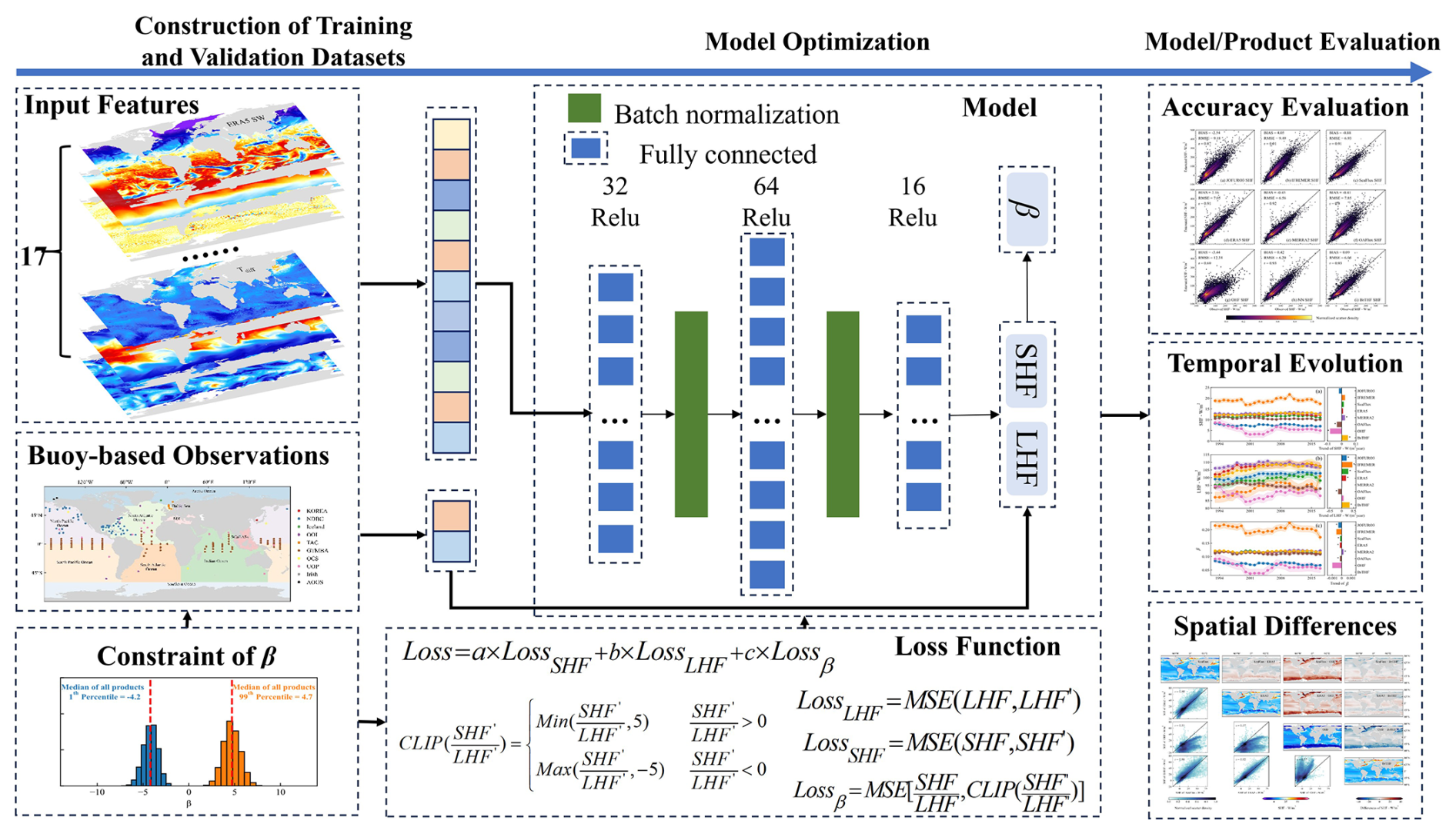
Figure 1 Flowchart of the generation of a global product of air–sea SHF, LHF and β by the BrTHF model.

2.1 Air-sea turbulent heat fluxes observation datasets

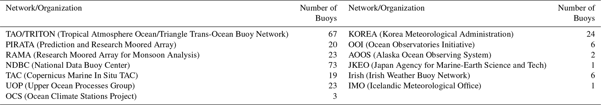
To obtain the buoy-derived air–sea turbulent heat fluxes observations, the hourly or sub-hourly oceanic and atmospheric measurements including sea surface temperature (T_s), sea surface air temperature (T_a), sea surface wind speed (WS) and relative humidity (RH) were firstly collected at 268 buoys covering a variety of ocean basins from 13 organizations or networks. Detailed information about the buoy sources and the number of buoys from each provider is summarized in Table 1.

Table 1 Summary of f buoys used in this study.

For certain buoys lacking RH measurements [e.g. buoys from NDBC (National Data Buoy Center) provided dew point temperature (DEW) rather than RH], the RH was computed using DEW and T_a. To ensure the quality of the measurements, we filtered the records based on the quality control recommendations provided by the data providers. Further refinement was also made by removing the questionable values that exceeded three standard deviations (3σ) for each variable at individual buoys.

Once the data was cleaned, daily mean aggregation was applied to the oceanic and atmospheric measurements. Given the varying temporal resolutions of the measurements (e.g. NDBC provided hourly observations before 2005 and 10 min observations thereafter), we only retained the daily mean data when the fraction of the valid hourly or sub-hourly observations exceeded 80 % on a given day.

After the above mentioned data preprocessing, the daily buoy-derived air–sea turbulent heat fluxes (SHF and LHF) observations were then calculated using the daily oceanic and atmospheric measurements combined with the version 3.5 of Coupled Ocean-Atmosphere Response Experiment (COARE3.5) model (Edson et al., 2013) (https://github.com/NOAA-PSL/COARE-algorithm, last access: 18 March 2023) with the cool-skin and warm-layer calculation switched off. The configuration follows the practice adopted by Pacific Marine Environmental Laboratory for producing daily air–sea turbulent heat flux products (https://www.pmel.noaa.gov/tao/drupal/flux/documentation-lw.html, last access: 31 March 2026) at Global Tropical Moored Buoy Array (TAO/TRITON, PIRATA, and RAMA) Note that outliers of β present in the observations are likely associated with uncertainties in the model-derived estimates and input data. Considering that such outliers can severely impede model training and evaluation, it was necessary to constrain β within a reasonable range to enable simultaneous high-accuracy estimation of SHF, LHF, and β. Therefore, following the air–sea turbulent heat fluxes computations, we further made quality control on the derived SHF and LHF observations to exclude the abnormal records, by filtering the observations based on the range of daily β values determined from seven widely-used flux products. Specifically, we calculated the cumulative distribution of daily β for each product and their ensemble (across all products). The medians of the 1st and 99th percentiles, approximately −5 and 5, respectively, were selected as the minimum and maximum of valid daily β, as shown in Fig. S1 in the Supplement. In total, this study compiled 463 585 observations of valid daily air–sea turbulent heat flux from 197 buoy stations (Fig. 2 and Table S1) in the Arctic Ocean, Pacific Ocean, Atlantic Ocean and Indian Ocean.

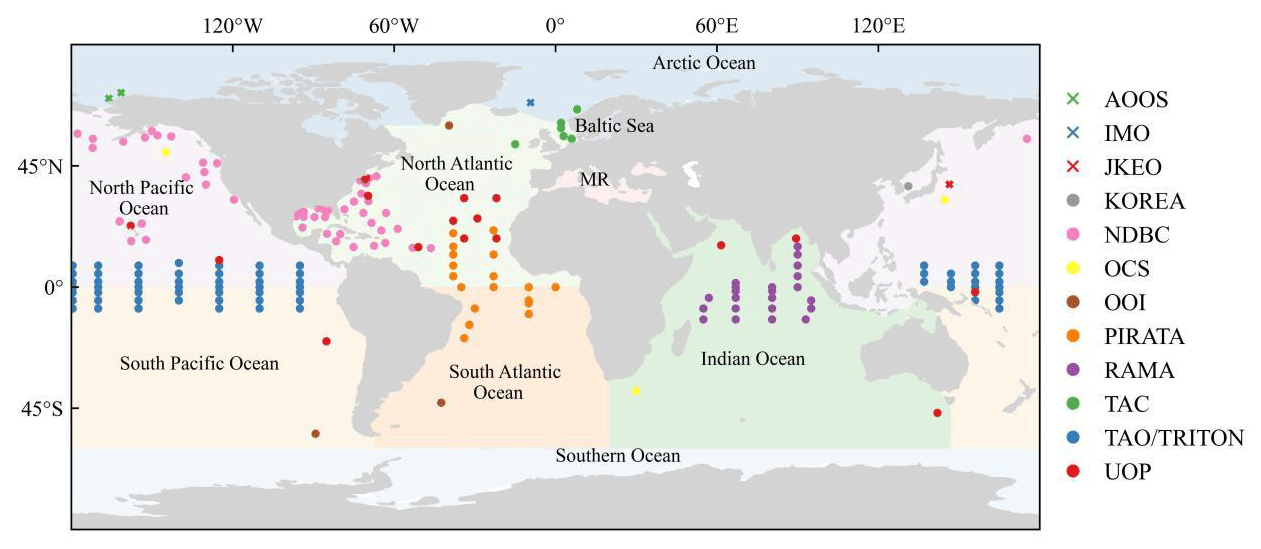
Figure 2 Geographic locations of 197 buoy sites from 12 organizations or networks involved in this analysis including TAO/TRITON, PIRATA, RAMA, NDBC, TAC, UOP, OOI, AOOS, KOREA, OCS, JKEO and IMO. The boundaries of global land and open oceans were sourced from the Natural Earth dataset (https://www.naturalearthdata.com/downloads/, last access: 8 January 2025) and the Global Oceans and Seas dataset (https://www.marineregions.org/sources.php, last access: 8 January 2025), respectively. Abbreviations MR refers to the Mediterranean Region. It should be noted that the Caspian Sea was not included within the boundaries of the open oceans and is shown in white.

Finally, the quality-controlled observations were collected to train and validate the BrTHF model. Note that the COARE-based observations at the buoy stations have already been widely applied as a benchmark for global air–sea turbulent heat flux product development and evaluation (Bentamy et al., 2017; Chen et al., 2020b; Tang et al., 2024; Weller et al., 2022)

2.2 Learning datasets and state-of-the-art products

2.2.1 Learning datasets for training the neural network

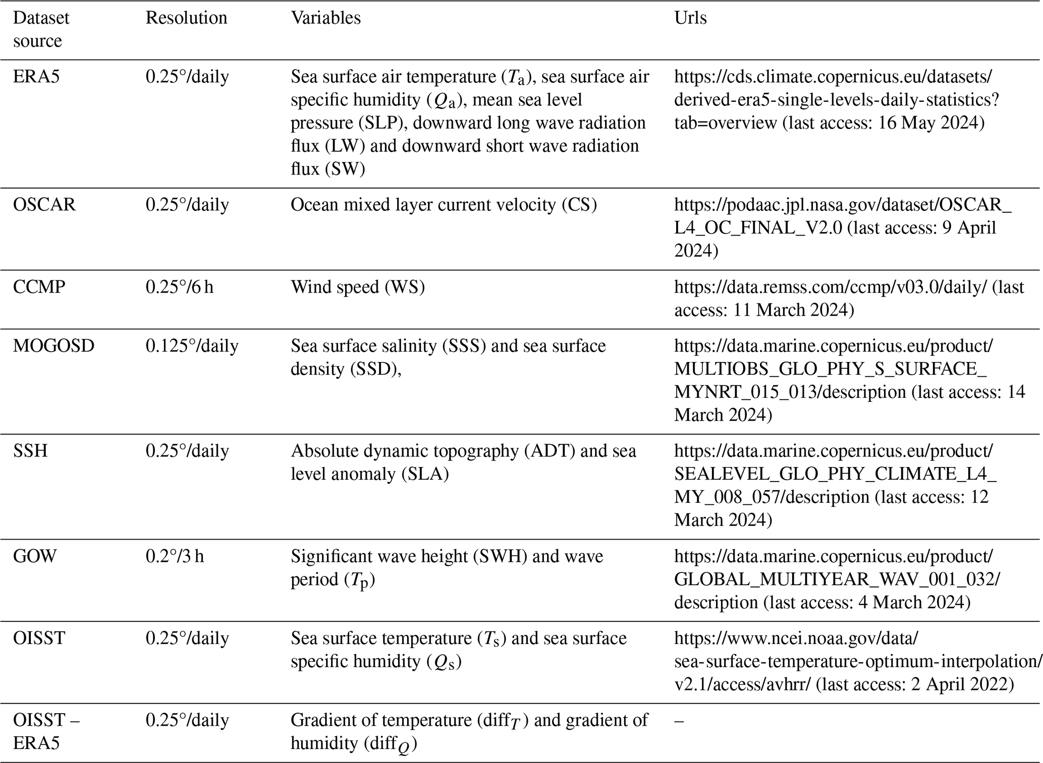
Learning variables were carefully selected based on their potential impacts on the variations of the air–sea turbulent heat fluxes (Grist et al., 2016; Kudryavtsev et al., 2014; Myslenkov et al., 2021; Song, 2020, 2021; Yan et al., 2024) to conduct the feature selection (see Sect. 2.3.1). These variables include T_a, sea surface air specific humidity (Q_a), Mean Sea Level Pressure (SLP), Downward Long Wave Radiation Flux (LW), Downward Short Wave Radiation Flux (SW), T_s, sea surface specific humidity (Q_s), Absolute Dynamic Topography (ADT), Sea Level Anomaly (SLA), Sea Surface Salinity (SSS), Sea Surface Density (SSD), Ocean Mixed Layer Current Velocity (CS), WS, Significant Wave Height (SWH), Wave period (T_p), as well as gradient of temperature (diff_T) calculated using the T_s and T_a, and gradient of humidity (diff_Q) calculated using the Q_s and Q_a.

Datasets of these learning variables were collected from multiple publicly available sources, as summarized in Table 2 and were used as the input features for training the neural network. The Multi Observation Global Ocean Sea Surface Salinity and Sea Surface Density (MOGOSD) dataset and Global Ocean Waves (GOW) Reanalysis dataset were spatially resampled to a 0.25° resolution using mean aggregation, while temporal mean aggregation to daily values was applied to the GOW dataset (originally at 3 h resolution) and Cross-Calibrated Multi-Platform (CCMP) wind vector analysis dataset (6 h resolution). Additionally, a daily ERA5 sea-ice mask was applied to the datasets to mitigate the impact of sea ice.

Table 2 Summary of learning datasets used in this study.

2.2.2 State-of-the-art products for inter-comparison

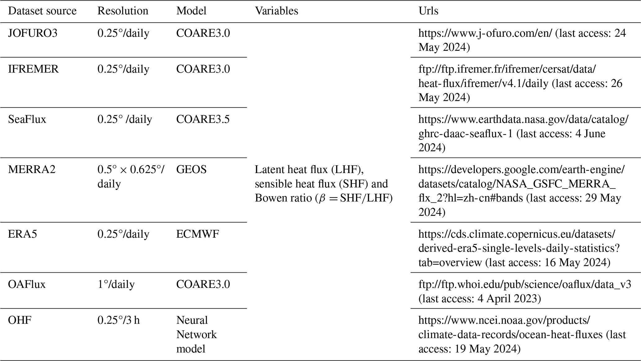
Seven widely used air–sea turbulent heat flux products, involving remote sensing-based JOFURO3, IFREMER and SeaFlux, as well as reanalysis-based ERA5 and MERRA2, hybrid-based OAFlux and machine learning-based OHF products were selected for inter-comparison, as summarized in Table 3.

The remote sensing-based JOFURO3, IFREMER, and SeaFlux products were developed by the Japanese Ocean Flux Data Sets under the Remote Sensing Observations (J-OFURO) research project, the Institute Français de Recherche pour l'Exploitation de la Mer (IFREMER), and the NASA Global Hydrology Resource Center (GHRC) Distributed Active Archive Center (DAAC), respectively. The reanalysis-based ERA5 and MERRA2 products were developed by the ECMWF and NASA Global Modeling and Assimilation Office (GMAO), respectively. The hybrid-based OAFlux and machine learning-based OHF products were developed or published by the Woods Hole Oceanographic Institution (WHOI) and NOAA Ocean Surface Bundle (OSB) Climate Data Record (CDR), respectively. With the exception of the OHF product calculating SHF and LHF simultaneously using a NN model without a constraint, all other products employed bulk aerodynamic methods to estimate SHF and LHF. The JOFURO3, IFREMER, and OAFlux products used the COARE3.0 model, while the SeaFlux used the COARE3.5 model. Differently, the ERA5 adopted the bulk aerodynamic method used by the ECMWF, and the MERRA2 used the method by the GEOS. These products provide SHF and LHF estimates at a 0.25° spatial resolution, except for the MERRA2 (0.5° × 0.625°) and OAFlux (1°). Additionally, most products provide daily SHF and LHF estimates, while only the OHF product provides estimates at a 3 h interval. For further inter-comparison, the daily mean aggregation was applied to the OHF product. More details about the seven products can be found in the review of Tang et al. (2024).

Table 3 Summary of the state-of-the-art air–sea turbulent heat flux products used for inter-comparison in this study.

2.3 Construction of the BrTHF model

2.3.1 Feature selection

The study employed a random forest (RF) model to evaluate the importance scores of 17 oceanic and atmospheric learning variables (with datasets collected in Sect. 2.2) for target variables (SHF and LHF), aiming to filter out less influential variables. As shown in Table S2, the variable importance assessment revealed that diff_T and diff_Q showed the highest importance scores (71.56 % and 49.93 %) for SHF and LHF modelling, respectively; additionally, WS exhibited the second highest importance for both SHF (10.19 %) and LHF (27.59 %) modelling. Building upon the importance evaluation and through careful screening of highly correlated variables, we ultimately selected 11 key environmental features for subsequent air–sea turbulent heat flux modelling including SLP, LW, SW, SSS, ADT, CS, WS, SWH, T_p, diff_Q, and diff_T.

2.3.2 Model construction and optimization

We selected the NN technique to build the BrTHF model due to its strong ability to capture the complex nonlinear relationships between the multiple inputs and multiple-target variables with high accuracy (Zhou et al., 2024; Fu et al., 2023; Cummins et al., 2023, 2024). Additionally, the technique enables the seamless integration of physical constraints, improving the reasonableness of the results (Zhou et al., 2024; Zhao et al., 2019; Shang et al., 2023).

In order to estimate the SHF and LHF with high accuracy in a physics-consistency framework, the β(= $\mathrm{SHF}/\mathrm{LHF}$) physical constraint was incorporated into the NN model using the custom multiple-objects (SHF, LHF and β) loss function as follows:

$$\begin{array}{}\text{(1)}& \mathrm{Loss}=a\times {\mathrm{Loss}}_{\mathrm{SHF}}+b\times {\mathrm{Loss}}_{\mathrm{LHF}}+c\times {\mathrm{Loss}}_{\mathit{\beta }}\end{array}$$

Loss_SHF, Loss_LHF and Loss_β represent the Mean Squared Error (MSE) of SHF, LHF and β, respectively. They were weighted using the factors of a (SHF), b (LHF) and c (β) to balance the different magnitudes of loss during optimization. To prevent potential gradient explosion during model training, predicted β[SHF${}^{\prime }/{\mathrm{LHF}}^{\prime }$, calculated using the predicted SHF (SHF^′) and LHF (LHF^′)] values were clipped within the observed range of β (from −5 to 5) during training:

$$\begin{array}{}\text{(2)}& {\displaystyle }\mathrm{CLIP}\left({\displaystyle \frac{{\mathrm{SHF}}^{\prime }}{{\mathrm{LHF}}^{\prime }}}\right)=\left\{\begin{array}{l}\mathrm{Min}\left(\frac{{\mathrm{SHF}}^{\prime }}{{\mathrm{LHF}}^{\prime }},\mathrm{5}\right)\frac{{\mathrm{SHF}}^{\prime }}{{\mathrm{LHF}}^{\prime }}>\mathrm{0}\\ \mathrm{Max}\left(\frac{{\mathrm{SHF}}^{\prime }}{{\mathrm{LHF}}^{\prime }},-\mathrm{5}\right)\frac{{\mathrm{SHF}}^{\prime }}{{\mathrm{LHF}}^{\prime }}<\mathrm{0}\end{array}\right.\text{(3)}& {\displaystyle }{\mathrm{Loss}}_{\mathit{\beta }}=\mathrm{MSE}\left({\displaystyle \frac{\mathrm{SHF}}{\mathrm{LHF}}},\mathrm{CLIP}\left({\displaystyle \frac{{\mathrm{SHF}}^{\prime }}{{\mathrm{LHF}}^{\prime }}}\right)\right)\end{array}$$

Finally, after optimization, the final weights (a, b and c) for SHF, LHF, and β were set to 5, 1, and 250, respectively. The model was constructed using the Python TensorFlow library and consisted of one input layer, three fully connected hidden layers, two Batch Normalization layers applied after the first and second hidden layers, and one output layer. The numbers of neurons in the three hidden layers were 32, 64, and 16, respectively and the activation function of Leaky Rectified linear unit (ReLU) was used throughout the model.

To illustrate the superiority of the BrTHF model in terms of accuracy and physical consistency, another physics-free NN models, trained without integrating the β constraint, were also constructed to predict SHF and LHF separately for further comparison, where β was calculated to be $\mathrm{SHF}/\mathrm{LHF}$.

2.4 Evaluation strategy

A spatial 10-fold cross-validation was employed to assess the performance of the BrTHF model for estimating air–sea SHF, LHF and β. Compared to the traditional 10-fold cross-validation, which randomly split all samples into ten folds and thus may result in overlapping spatial samples between training and validating datasets, the spatial 10-fold cross-validation was conducted in a relatively independent spatial distribution and can provide a more robust and generalizable evaluation.

Specifically, first, all buoy sites were randomly split into ten folds. Then, each fold was in succession selected as the validation dataset and the remaining nine folds were used as the training dataset.

The metrics used to evaluate the performance of the models include: (1) the mean bias error (BIAS); (2) the root mean squared error (RMSE); (3) the correlation coefficient (r).

$$\begin{array}{}\text{(4)}& {\displaystyle }\mathrm{BIAS}={\displaystyle \frac{\mathrm{1}}{n}}\sum _{i=\mathrm{1}}^n\left({\widehat{y}}_i-y_i\right)\text{(5)}& {\displaystyle }\mathrm{RMSE}=\sqrt{{\displaystyle \frac{\mathrm{1}}{n}}\sum _{i=\mathrm{1}}^n{\left({\widehat{y}}_i-y_i\right)}^{\mathrm{2}}}\text{(6)}& {\displaystyle }r={\displaystyle \frac{\sum _{i=\mathrm{1}}^n\left[\right({\widehat{y}}_i-\stackrel{\mathrm{‾}}{\widehat{y}}\left)\right(y_i-\stackrel{\mathrm{‾}}{y}\left)\right]}{\sqrt{\sum _{i=\mathrm{1}}^n{\left({\widehat{y}}_i-\stackrel{\mathrm{‾}}{\widehat{y}}\right)}^{\mathrm{2}}\sum _{i=\mathrm{1}}^n{\left(y_i-\stackrel{\mathrm{‾}}{y}\right)}^{\mathrm{2}}}}}\end{array}$$

where n is the number of samples, ${\widehat{y}}_i$ and y_i are the estimated value and reference truth, $\stackrel{\mathrm{‾}}{\widehat{y}}$ and $\stackrel{\mathrm{‾}}{y}$ are the mean of ${\widehat{y}}_i$ and y_i, respectively. These metrics – BIAS, RMSE, and r – comprehensively evaluate model performance, representing systematic deviation, dispersion between observations and estimates, and the strength and direction of the linear relationship, respectively. Note that RMSE and r can be sensitive to extreme values, particularly for the β, which is a ratio-based variable and may exhibit unrealistically large magnitudes under near-zero flux conditions. To ensure a fair evaluation, model performance is assessed both with all samples retained and with extreme β values excluded in subsequent analyses. This dual evaluation allows us to quantify overall model performance while explicitly accounting for the influence of rare extreme cases.

3 Results and discussion

3.1 Spatial ten-fold cross-validation of the models

3.1.1 Overall accuracy

Figures 3, 4 and 5 present the normalized scatter density plots of the estimated daily SHF, LHF and β from the BrTHF and physics-free NN models, as well as the seven air–sea turbulent heat flux products against the observations obtained from 197 globally distributed buoys by the spatial ten-fold cross-validation strategy.

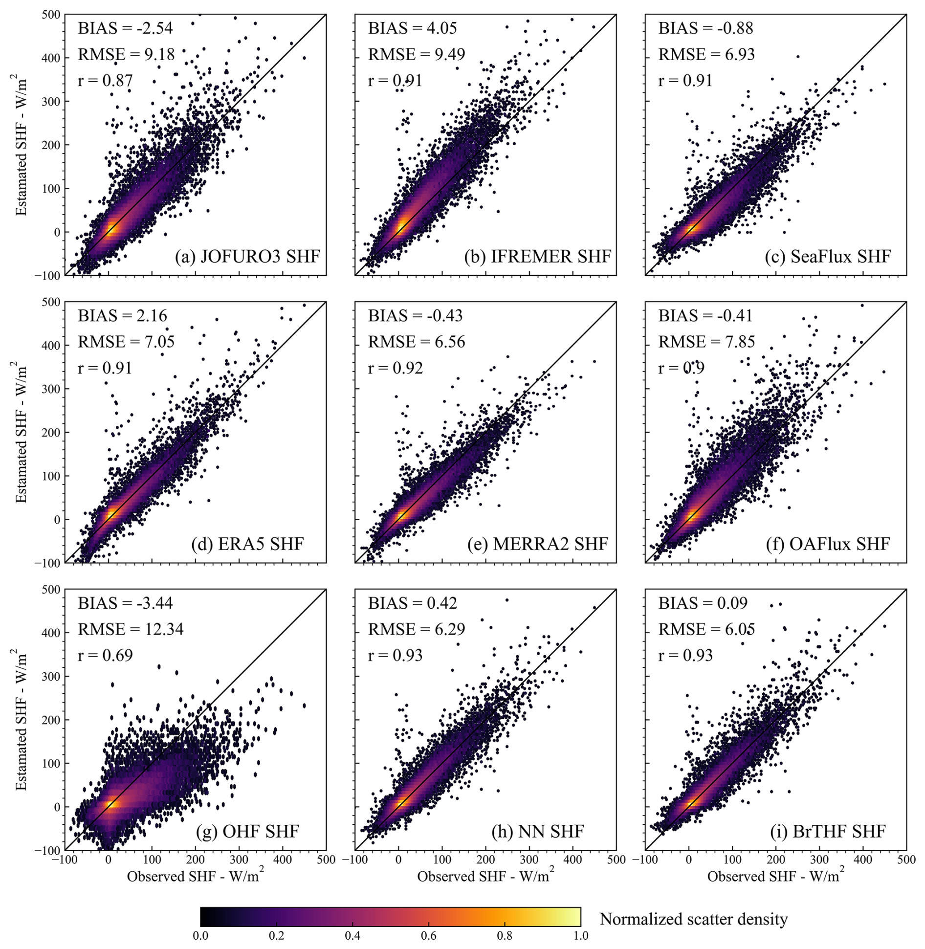
Figure 3 Normalized scatter density plots of estimated SHF from the BrTHF model, the physics-free NN models and seven air–sea turbulent heat flux products against the observed SHF obtained from 197 global distributed buoys.

Figure 4 Same as Fig. 3 but for LHF.

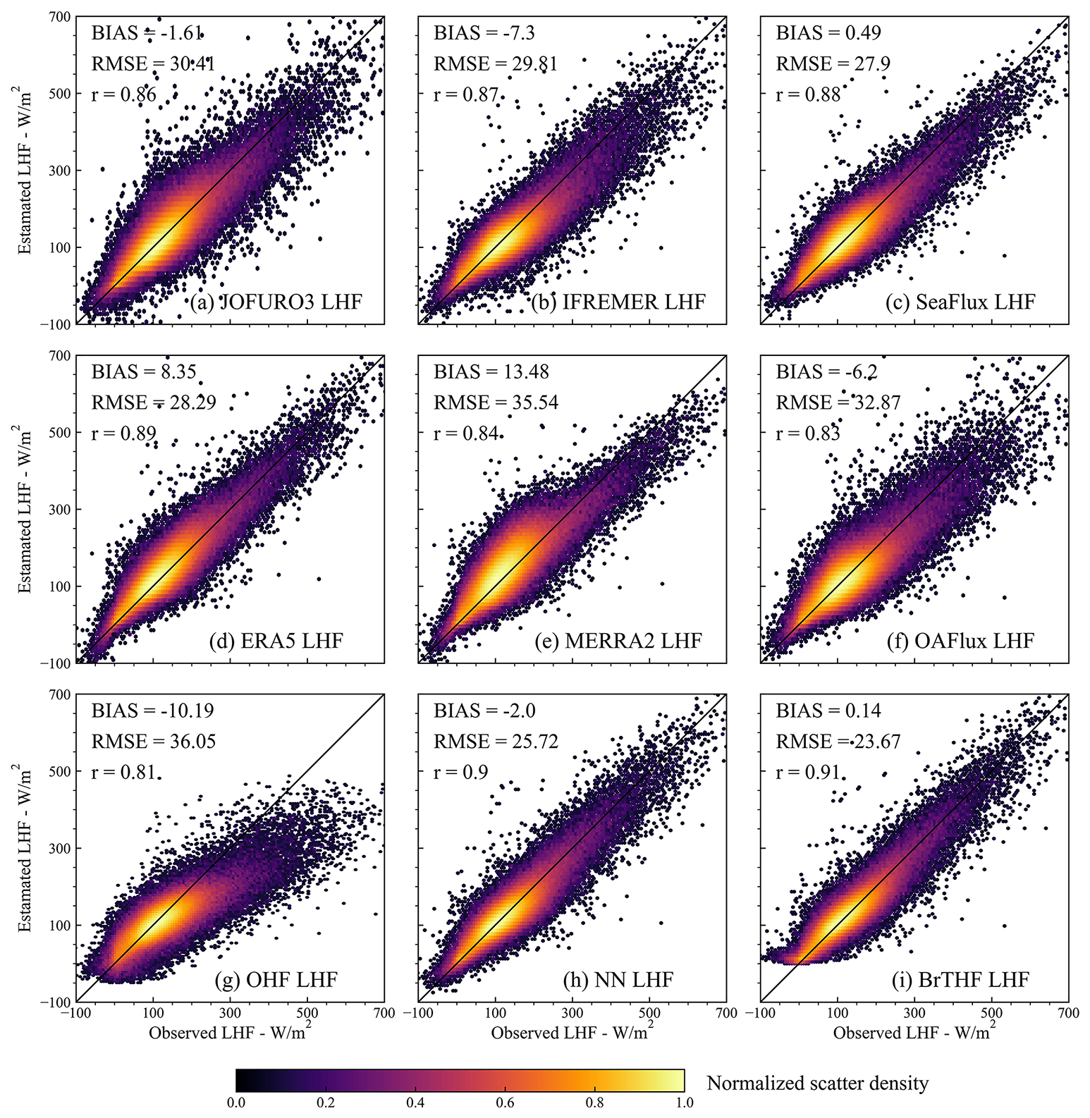
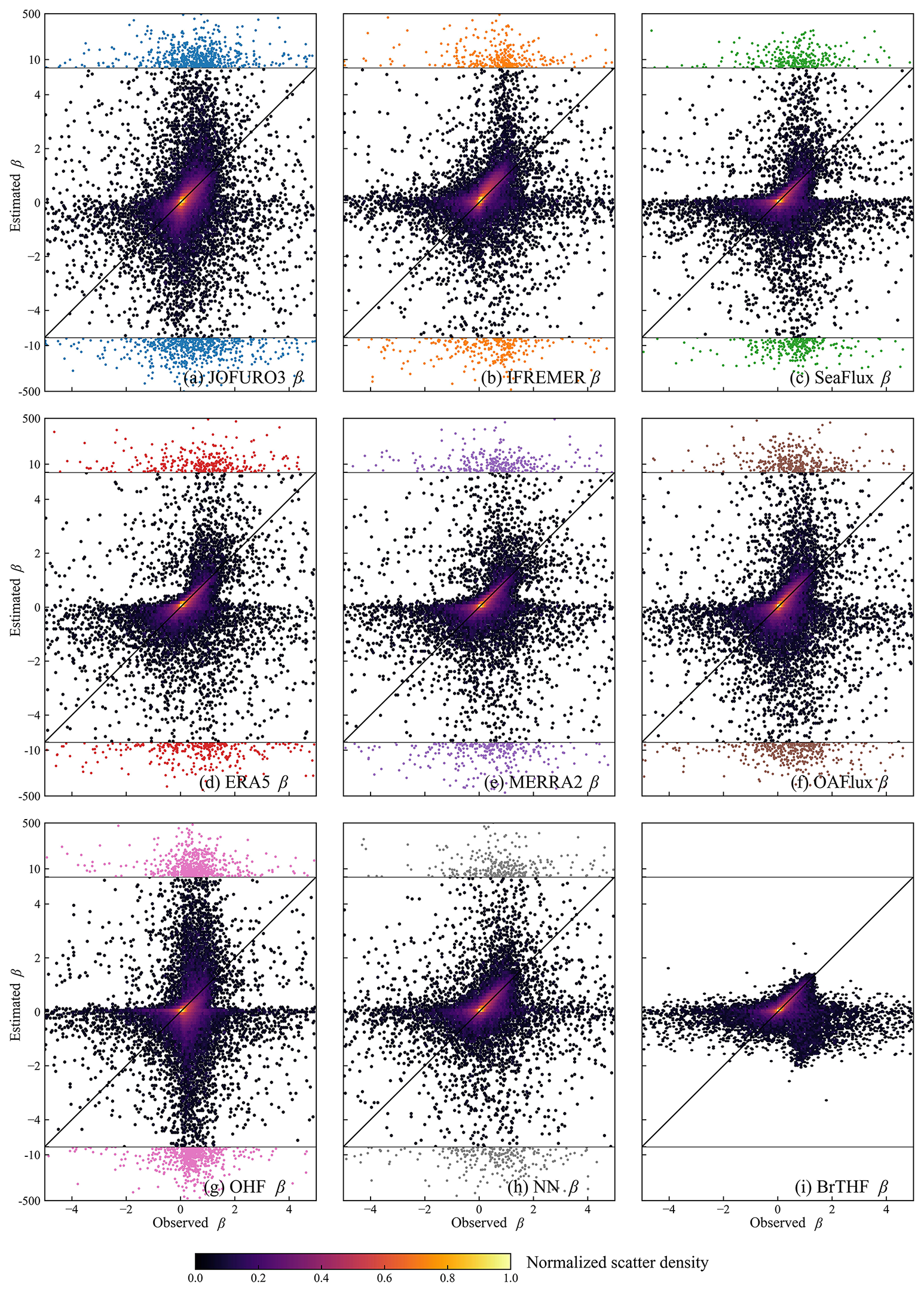
Figure 5 Same as Fig. 3 but for β. The samples out of the ranges of observed β (−5 $\le \mathit{\beta }\le$ 5) were colored in blue, orange, green, red, purple, brown, pink and gray for JOFURO3, IFREMER, SeaFlux, ERA5, MERRA2, OAFlux, OHF products and the physics-free NN models, respectively. The statistical metrics could be found in Table S3 and Fig. 6.

Most models and products showed data distributions closely aligned with the observed SHF, with the majority of samples clustered around the 1:1 line. The BrTHF model slightly overestimated SHF with a BIAS of 0.09 W m⁻², whereas the physics-free NN models, and ERA5 and IFREMER products showed more pronounced overestimations (from 0.42 to 4.05 W m⁻²). In contrast, the remaining five products exhibited notable underestimations (from −3.44 to −0.41 W m⁻²). As illustrated in Fig. 6, the variability of estimated SHF from the BrTHF and the physics-free NN models and ERA5 product closely matched the observed SHF, all with a Standard Deviation (STD) of approximately 16 W m⁻². Notably, the BrTHF model achieved the lowest RMSE (6.05 W m⁻²), outperforming both the physics-free NN models (6.29 W m⁻²) and the seven air-sea turbulent heat flux products (ranging up to 12.34 W m⁻² for OHF). Additionally, the BrTHF model combined with the physics-free NN models yielded the highest values of r (0.93), surpassing all seven other products. In summary, the BrTHF model showed the best overall performance in estimating SHF among all the models and products.

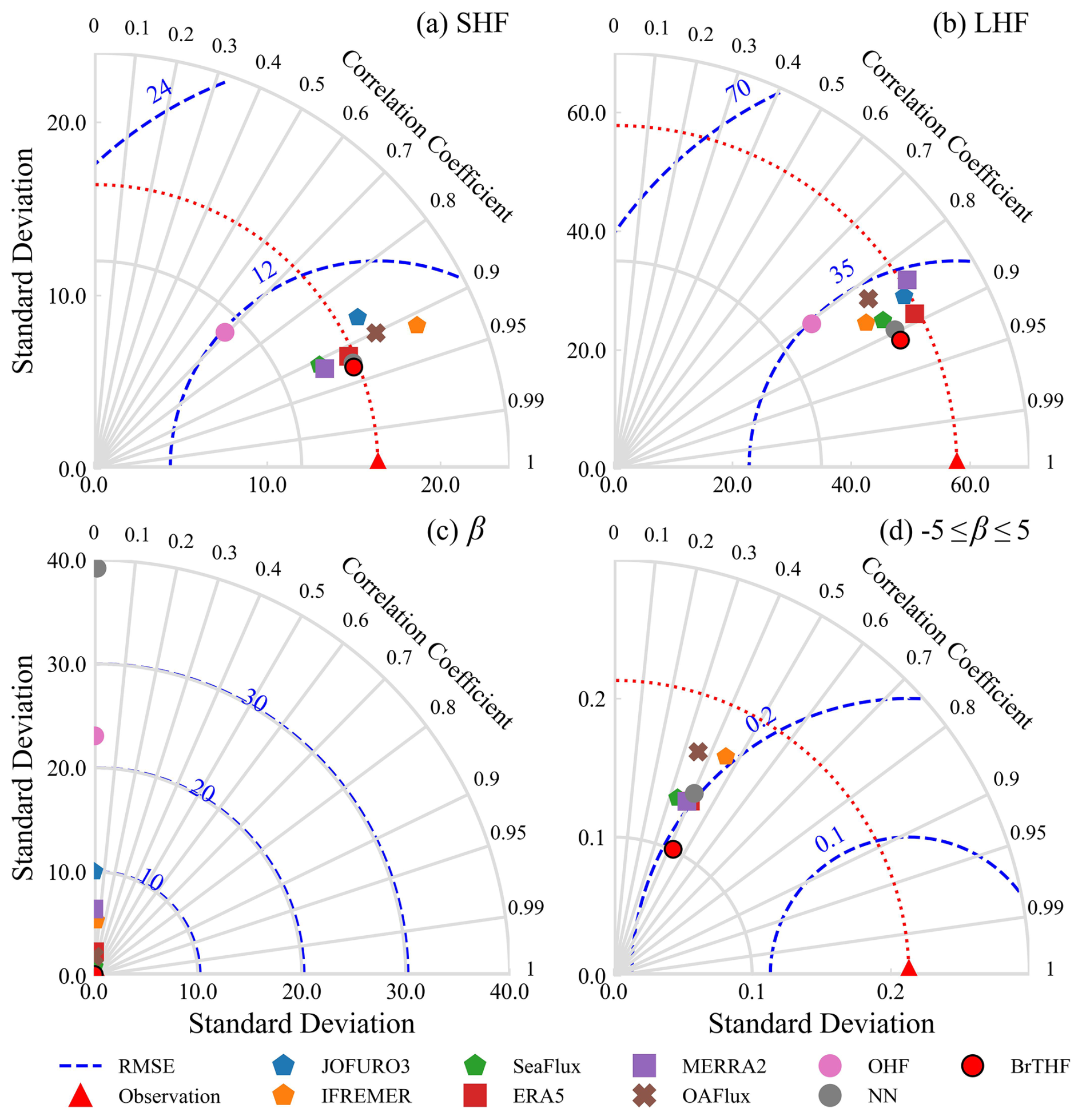
Figure 6 Taylor diagrams of the validation of estimated daily SHF (a), LHF (b), β (c) and β (−5 $\le \mathit{\beta }\le$ 5, d) from the BrTHF model, the physics-free NN models and the seven products against the in-situ observations.

For LHF, similar to the results for SHF, the BrTHF model demonstrated the best agreement with observations, achieving the lowest RMSE (23.67 W m⁻²) and the highest value of r (0.91). Compared to the physics-free NN models and seven products, the BrTHF model reduced RMSE by 2.05 W m⁻² (physics-free NN models) to 12.38 W m⁻² (OHF) and improved r by 0.01 (physics-free NN model) to 0.1 (OHF). Additionally, the BrTHF model showed a slight overestimation of LHF (BIAS = 0.14 W m⁻²), lower than that of the SeaFlux, MERRA2, and ERA5 products. In contrast, the remaining products (JOFURO3, IFREMER, OAFlux, and OHF), along with the physics-free NN models, underestimated LHF, with the BIAS values ranging from −10.19 W m⁻² (OHF) to −1.61 W m⁻² (JOFURO3).

The BrTHF model exhibited a significantly different distribution of β compared to the physics-free NN models and the seven products, as shown in Fig. 5. The β estimates from the BrTHF model consistently fell within the observed range of −5 to 5, while the physics-free NN model and the seven products occasionally produced estimates outside this range. Specifically, approximately 0.9 % of β estimates from both the physics-free NN model and the seven products were out of range. The extreme positive and negative β estimates were found in the OHF (β= 14 997) and physics-free NN models (β= −25 703) products, respectively. The abnormal β estimates significantly impacted the accuracy of the physics-free NN models and the seven products as Fig. 6 indicated. When excluding the abnormal β samples from the physics-free NN models and seven products, the RMSEs ranged from 0.17 (physics-free NN models and SeaFlux) to 0.26 (OHF), with values of r ranging from 0.13 (OHF) to 0.46 (IFREMER), as shown in Fig. 6 and Table S3. However, when all estimates were considered, the performances of these model and products deteriorated sharply, with RMSEs rising from 0.87 (SeaFlux) to 39.21 (physics-free NN models), and values of r dropping from 0.06 (SeaFlux) to 0 (JOFURO3, MERRA2 and OHF). In contrast, the BrTHF model maintained robust outperformance, with the lowest RMSEs of 0.22 and 0.15, and higher r values of 0.25 and 0.43, both before and after removing the abnormal β samples from the physics-free NN models and the seven products. Notably, the BIAS values remained stable (ranging from −0.04 to 0.04) for all models and products, regardless of whether the abnormal samples were excluded.

3.1.2 Accuracies across oceans

To better understand the accuracy of SHF, LHF and β estimates from the BrTHF and physics-free NN models, as well as the seven products in different oceans, we conducted an additional evaluation by categorizing the observations according to the belonging ocean basins, as shown in Fig. 7. The major ocean boundaries, obtained from Marine Regions (https://www.marineregions.org/, last access: 31 March 2026), were used to define the ocean basins, which include the Arctic Ocean, South Pacific Ocean, North Pacific Ocean, South Atlantic Ocean, North Atlantic Ocean, and Indian Ocean.

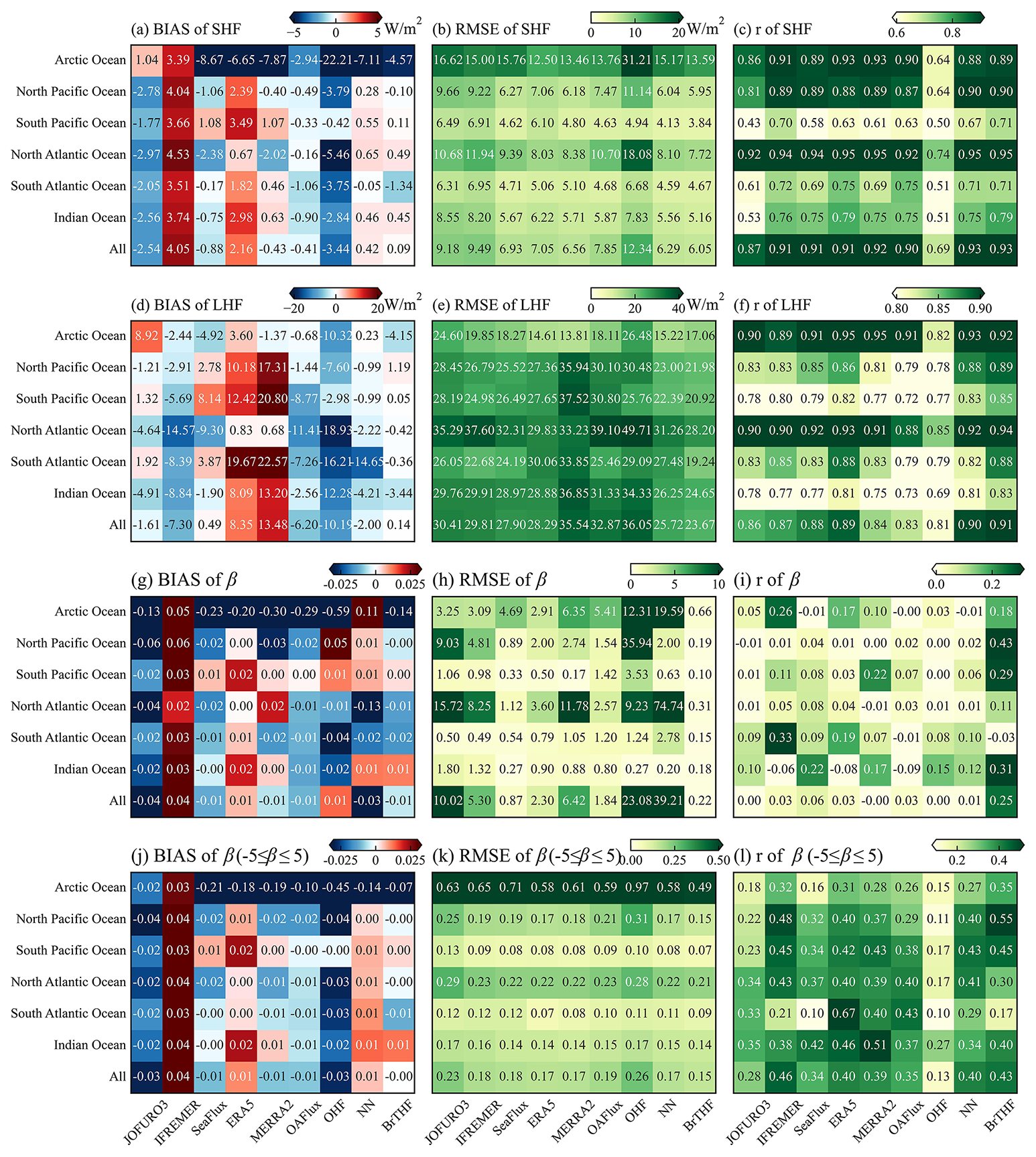
Figure 7 Heatmaps of BIAS, RMSE and r metrics for the validation of estimated daily SHF (a–c), LHF (b–e), β (f–i) and β (−5 $\le \mathit{\beta }\le$ 5, j–l) from the BrTHF model, the physics-free NN models and the seven products against the in-situ observations across different ocean basins. It should be noted that the statistical metrics for each ocean basin were calculated using observations from the available buoys within the corresponding basin.

For SHF, the BrTHF model exhibited overestimations in the South Pacific Ocean, North Atlantic Ocean, and Indian Ocean, while it underestimated SHF in the remaining three ocean basins. The values of BIAS ranged from −4.57 W m⁻² in the Arctic Ocean to 0.49 W m⁻² in the North Atlantic Ocean. Furthermore, the BrTHF achieved the lowest RMSEs in most ocean basins, ranging from 3.84 W m⁻² in the South Atlantic Ocean to 7.72 W m⁻² in the North Atlantic Ocean, except in the Arctic Ocean where the RMSE of 13.59 W m⁻² was higher than those of the ERA5 (12.5 W m⁻²) and MERRA2 (13.46 W m⁻²) products, as shown in Fig. 7b. Correlation analysis also demonstrated the robust performance of the BrTHF model in estimating SHF, with values of r exceeding 0.89 in most ocean basins, except for ocean basins in the Southern Hemisphere (ranging from 0.71 to 0.79) where the values of r for all models and products were reduced.

For LHF, the values of BIAS of the BrTHF model ranged from −4.15 W m⁻² in the Arctic Ocean to 1.19 W m⁻² in the North Pacific Ocean. In comparison, the BrTHF model showed more pronounced underestimations in the Arctic Ocean and Indian Ocean. Additionally, the BrTHF model outperformed the physics-free NN models and the seven products across most ocean basins, achieving the lowest RMSEs (ranging from 17.06 W m⁻² in the Arctic Ocean to 28.20 W m⁻² in the North Atlantic Ocean) and the highest values of r (ranging from 0.83 in the Indian Ocean to 0.94 in the North Atlantic Ocean) except for the Arctic Ocean where the value of r was 0.01 less than the physics-free NN models and the RMSEs were 2.45, 3.25 and 1.84 W m⁻² higher than the ERA5 and MERRA2 products and the physics-free NN models, respectively. Combining the overall and regional evaluations, we find that, except for the OHF product, the relative performance of SHF and LHF among the seven products is generally consistent with Tang et al. (2024). The OHF product shows notable degradation, particularly in high-latitude oceans, which may be due to limitations in the training datasets (sparse and unevenly distributed in-situ observations) and model training strategy (randomly splitting all observations into training, validation, and test sets without accounting for spatial dependencies), leading to reduced generalizability.

The BrTHF model consistently performed better in estimating β across most ocean basins, both before and after removing the abnormal β samples that deviated from the observed range (−5 $\le \mathit{\beta }\le$ 5). In contrast, the physics-free NN models and the seven products did not perform as well. Specifically, the BrTHF model exhibited the lowest RMSEs in almost all ocean basins except in the South Atlantic Ocean after removing β outliers. Moreover, in terms of correlation analysis, the BrTHF model achieved higher values of r in most ocean basins before and after the removal of abnormal β samples, among all models and products.

3.2 Temporal variations in SHF, LHF and β

After spatial ten-fold cross-validation, we produced the daily 0.25° global air–sea turbulent heat flux products from 1993 to 2017 using a combination of the BrTHF model and learning datasets, and further made a comparison of the temporal variation (in this section), spatial distribution (in Sect. 3.3) and annual trend (in Sect. 3.4) of SHF, LHF and β estimates from the BrTHF product and those with the seven state-of-the-art global products. The selected period (from 1993 to 2017) was determined by the overlapping availability of input learning datasets.

Figure 8 illustrates the monthly area-weighted global means of SHF, LHF and β from 1993 to 2017 for the BrTHF product and seven state-of-the-art products. The BrTHF product exhibited similar bimodal patterns for SHF, LHF and β as the seven products, with peaks in December-January and May-June-July-August. In addition, the peak in May-June-July-August was less pronounced for SHF and β compared to that for LHF. The monthly area-weighted global means of SHF and β from the BrTHF product were higher than those of most products, except for the MERRA2 product in January, February, March, April, July, August and September, and the IFREMER product in all months. For LHF, the BrTHF showed lower values than the ERA5 and MERRA2 products across all months. Notably, the patterns of SHF and β from the OHF product, with the highest peak occurring in August and smoother intra-annual cycles, differed from those of the corresponding BrTHF product and the other six products developed using the bulk aerodynamic methods.

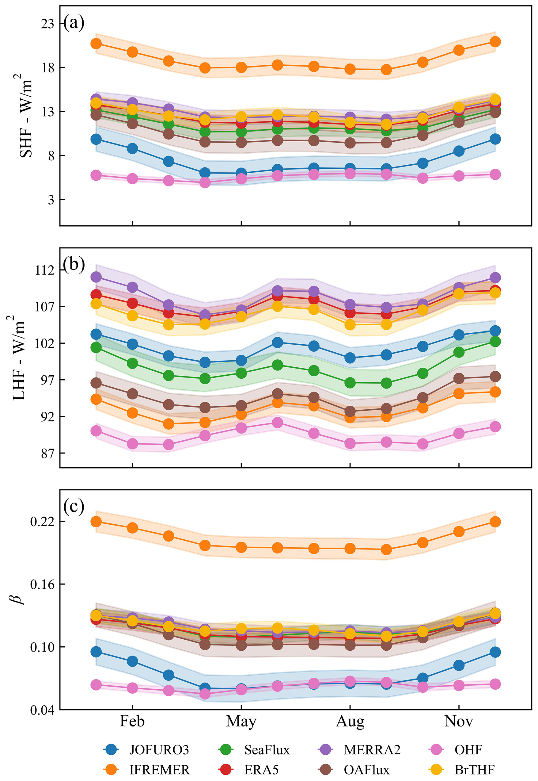
Figure 8 Intra-annual cycles of area-weighted global monthly mean of SHF (a), LHF (b) and β (c) from the eight products from 1993 to 2017. The shaded areas indicate ±1 standard deviation around the mean.

Figure 9 presents the temporal evolution of the area-weighted annual global mean of SHF, LHF and β from 1993 to 2017 for the eight products over ice-free oceans. The global mean annual SHF of the BrTHF product was 12.7 W m⁻², which was close to those of SeaFlux (11.6 W m⁻²), OAFlux (10.6 W m⁻²), MERRA2 (13 W m⁻²) and ERA5 (12.4 W m⁻²), whereas it significantly lower than that of IFREMER (18.8 W m⁻²) and higher than those of JOFURO3 (7.5 W m⁻²) and OHF (5.6 W m⁻²). Meanwhile, the BrTHF product exhibited the largest significant increase of SHF with the trend of 0.04 W m⁻² yr⁻¹ among all eight products, and showed similar temporal evolution as SeaFlux, MERRA2, ERA5 and OAFlux during the period from 1993 to 2017. As for LHF, the BrTHF exhibited a relatively high global mean annual value of 106.2 W m⁻², which was close to those of the ERA5 (107.3 W m⁻²) and MERRA2 (108.3 W m⁻²), and it was significantly higher than the rest of the products. Moreover, the growth of the BrTHF LHF was significant with a trend of 0.33 W m⁻² yr⁻¹, which was lower than the IFREMER but higher than the OAFlux, MERRA2, OHF, ERA5, JOFURO3 and SeaFlux, ranging from −0.14 W m⁻² yr⁻¹ to 0.4 W m⁻² yr⁻¹. Note that only the OAFlux product showed a negative trend of LHF from 1993 to 2017. For β, the BrTHF showed a similar temporal pattern to that of SHF, and most products concentrated within the narrow range of 0.11 to 0.12 for the annual values. The magnitude of annual β of the BrTHF was about 0.11, which was close to the OAFlux, SeaFlux, MERRA2 and ERA5, but significantly lower than the IFREMER and higher than the JOFURO3 and OHF. Moreover, in contrast to the significant increasing trends of LHF and SHF, negative trends of β were shown for most products. However, the BrTHF product exhibited a weak positive trend, which may be attributed to the relatively smaller differences between the SHF and LHF trends in BrTHF compared to those in other products.

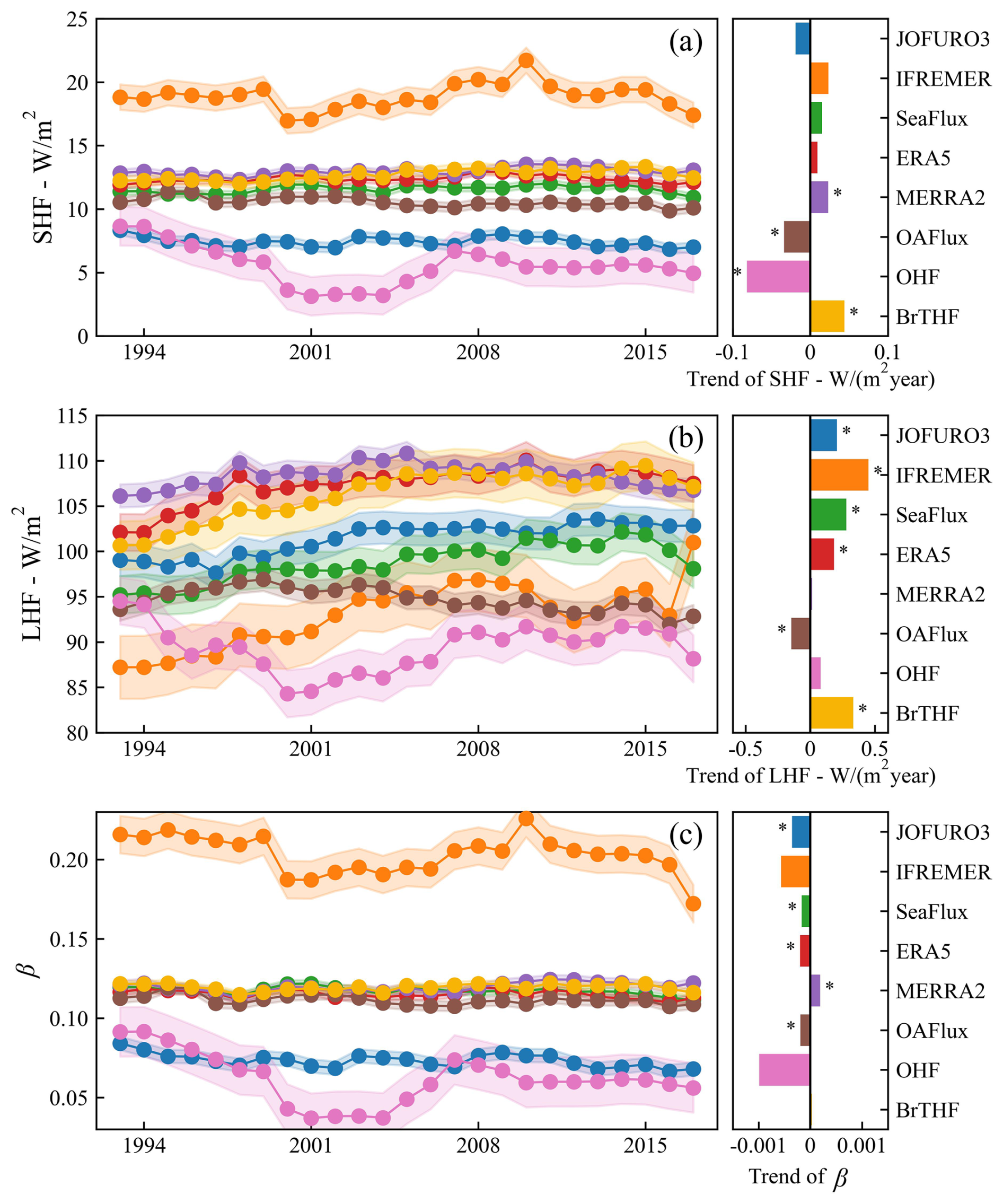
Figure 9 Inter-annual evolution of area-weighted global mean SHF (a–b), LHF (c–d) and β (e–f) from 1993 to 2017. The trends were calculated based on the Sen's slope method. The ^* in the sub-figures (b, d, f) represent the trend passed the Mann–Kendall significant test (p<0.05). The shaded areas indicate ±1 standard deviation around the mean.

3.3 Inter-comparison of the spatial pattern

We selected three representative products including the (reanalysis-based) ERA5, (remote sensing-based) SeaFlux, and (the machine learning-based) OHF products to evaluate the BrTHF product's ability in simulating global air–sea turbulent heat fluxes (SHF, LHF, and β) from 1993 to 2017. These products were chosen because they demonstrated relatively high accuracy within their respective categories (as shown in Sect. 3.1) and shared the same 0.25° spatial resolution with the BrTHF product.

Figure 10 presents the spatial distribution of multi-year mean of SHF from the SeaFlux, ERA5, BrTHF, and OHF products, along with their cross-comparisons. Overall, the BrTHF product exhibited strong consistency with ERA5 and SeaFlux products, with values of r exceeding 0.88, which was significantly higher than the consistency between SeaFlux and OHF (r = 0.33) and between ERA5 and OHF (r = 0.37). Spatially, the BrTHF, SeaFlux and ERA5 products all showed higher SHF (over 50 W m⁻²) in the Western Boundary Currents (WBCs, e.g. Kuroshio, Gulf Stream, Brazil Current and Agulhas Current) regions, whereas the OHF product yielded much lower SHF (∼ 25 W m⁻²). Additionally, the former three products captured pronounced SHF gradients in the Southern Ocean, features that were absent in the OHF product. SHF differences between BrTHF and SeaFlux/ERA5 remained within ±10 W m⁻² in most oceans. The BrTHF product exhibited slightly higher SHF values than SeaFlux in the Northern Hemisphere, whereas in the Southern Hemisphere – particularly over the Southern Ocean – the BrTHF showed relatively lower SHF. Compared to the ERA5 product, the BrTHF product yielded lower SHF in the equatorial zone, subtropical high-pressure regions and the Southern Ocean, but higher SHF in other areas, particularly in the North Pacific and the southern Indian Ocean.

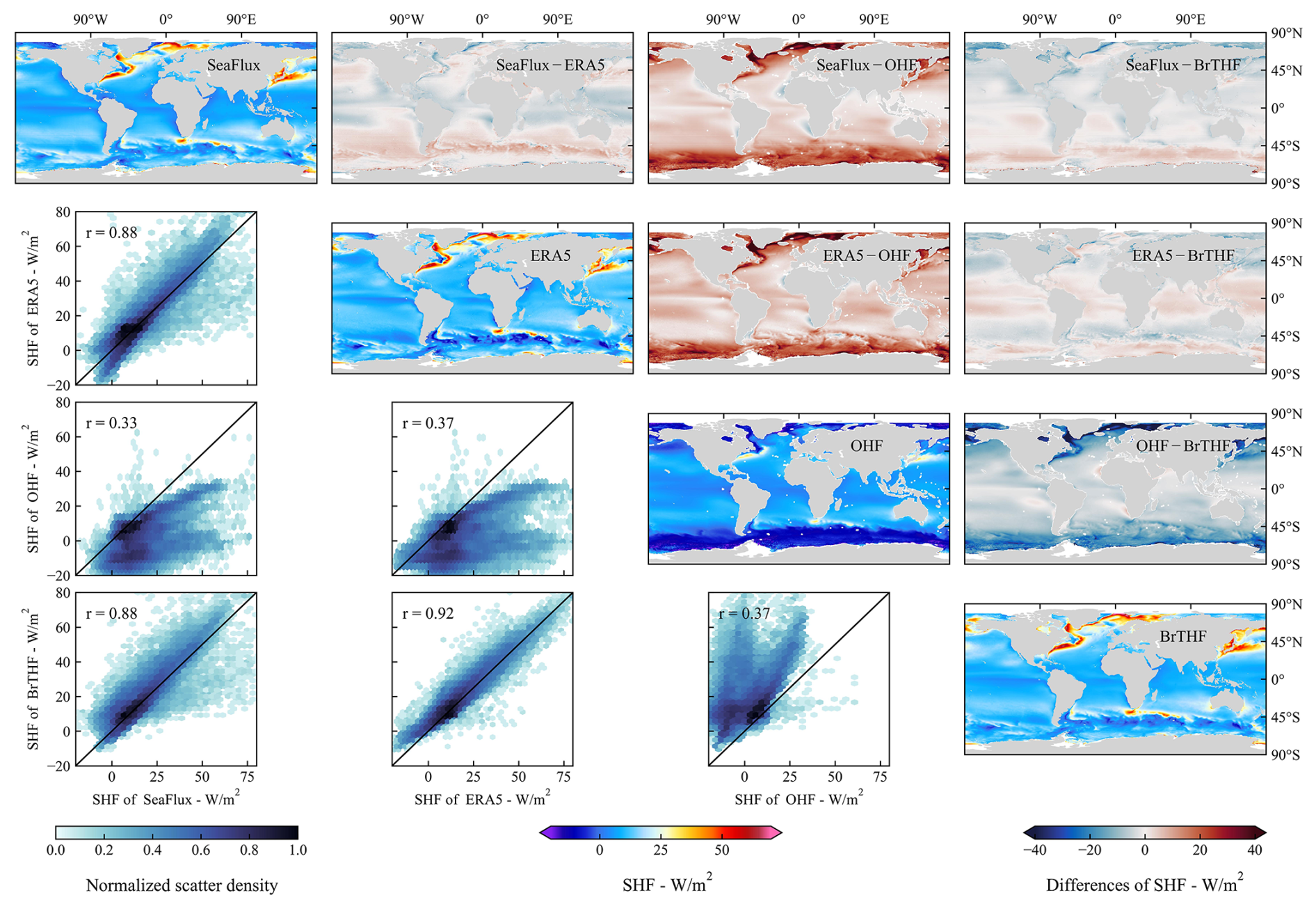
Figure 10 Inter-comparison of the spatial distributions of multi-year means of SHF among the SeaFlux, ERA5, OHF and BrTHF products from 1993 to 2017.

For LHF, the BrTHF and the three reference products exhibited more similar spatial distribution patterns, with the values of r exceeding 0.98, compared to the results for the SHF, as shown in Fig. 11. The higher LHF (over 150 W m⁻²) primarily occurred around the regions of WBCs and the sub-tropic highs, while lower LHF (below 50 W m⁻²) appeared in the Eastern Equatorial Pacific and Atlantic Warm Tongue and the oceans with latitudes higher than 45°. The spatial distribution of LHF in the BrTHF product generally agreed better with that of the ERA5 product, though the BrTHF showed significantly lower LHF in sub-tropic highs. Additionally, the BrTHF exhibited relatively lower LHF than the ERA5 over the Southern Ocean and the central North Atlantic. Compared to the SeaFlux, the BrTHF yielded slightly higher LHF in most oceans except the Southern Ocean and equatorial zones.

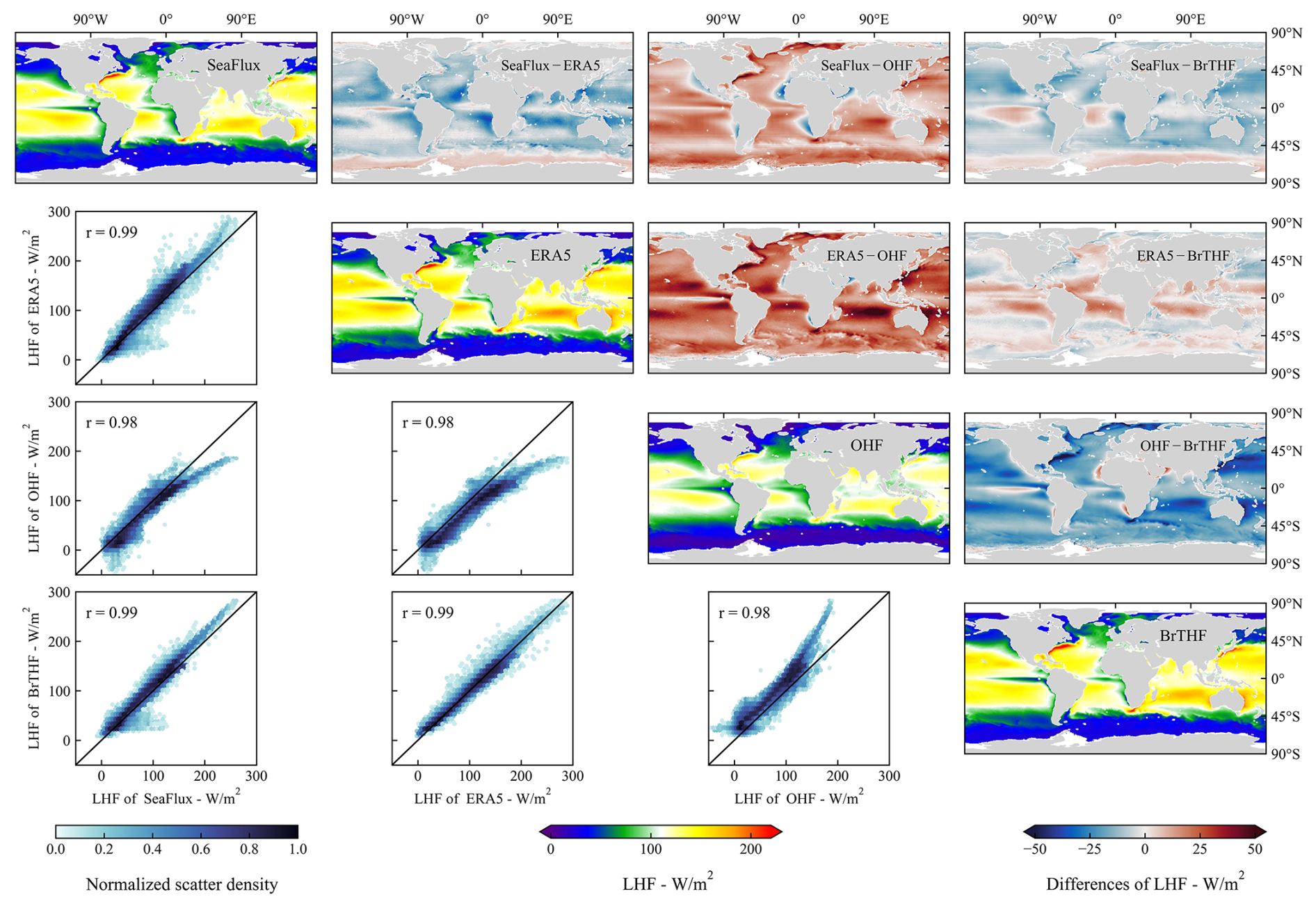
Figure 11 Same as Fig. 10 but for LHF.

For β, the BrTHF product demonstrated strong spatial correlation with the ERA5 and SeaFlux in multi-year mean distributions, with values of r exceeding 0.81. In contrast, the OHF showed a markedly different spatial pattern of β, exhibiting negative correlations when compared to the other three products. Spatially, the BrTHF product's β distribution aligned more closely with the SeaFlux, both displaying higher β (up to 1) in high-latitude oceans particularly in the Northern Hemisphere and the similar wavelike textures of β over the Southern Ocean's Antarctic Circumpolar Current zone. The differences between the BrTHF and OHF products were more evident. Specifically, the BrTHF product showed overall overestimation of β in the oceans where latitudes were larger than 45° compared to the OHF product.

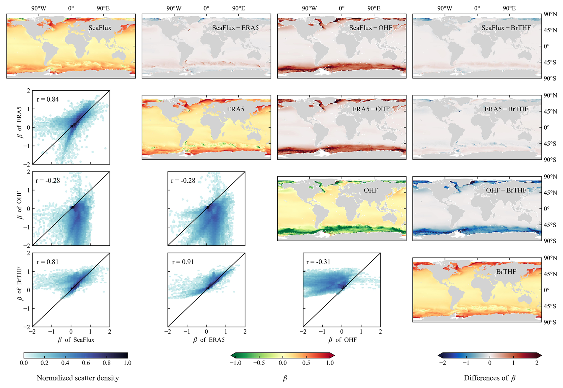
Figure 12 Same as Fig. 10 but for β.

3.4 Spatial pattern of trends in SHF, LHF and β from the BrTHF product

Figure 13 illustrates the spatial distribution of inter-annual trends of SHF, LHF and β in the BrTHF product from 1993 to 2017. The SHF showed increasing trends across 71.4 % of the oceans, with statistically significant increases in 26.2 % of regions. In contrast, decreasing trends were observed in 28.6 % of the oceans, with only 3 % showing significant reductions. Overall, the trends of zonal annual averages of SHF remained stable between 60° N to 45° S, with significant increases occurring southward and decreases northward. Specifically, moderate increases (∼ 0.2 W m⁻² yr⁻¹) dominated between 45° N and 45° S, while more pronounced increases (> 0.8 W m⁻² yr⁻¹) were observed in mid- and high-latitude oceans, including the Kara Sea, Gulf Stream, Baffin Bay, Brazil Current, Sea of Okhotsk, and Sea of Japan. Notable decreases (< −0.8 W m⁻² yr⁻¹) were concentrated in the Barents Sea and the central North Atlantic.

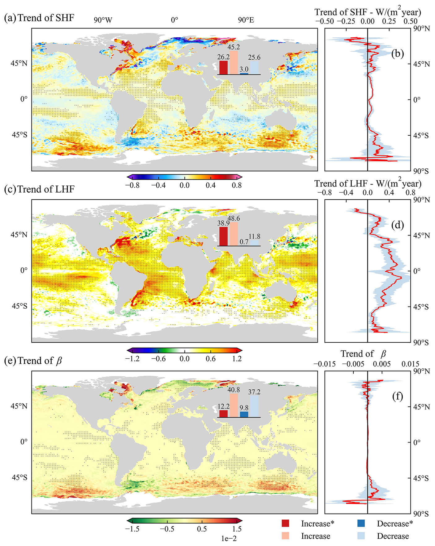
Figure 13 Spatial maps of inter-annual trends for SHF (a), LHF (c), and β (e) from the BrTHF product for the period 1993 to 2017. The trends were calculated using the Sen's slope method. Dotted areas indicate oceans where the p-value of the Mann–Kendall significance test is less than 0.05. Panels (b), (d) and (f) represent the inter-annual trends of zonal annual averages for SHF, LHF and β, respectively.

The LHF exhibited markedly different characteristics of the spatial distribution, with 87.5 % of oceans showing increasing trends (38.9 % were significant), versus 12.5 % decreasing (0.7 % were significant). In contrast to those of the SHF, the trends of zonal annual averages for LHF weakened poleward from the oceans of Equator. The substantial increases (> 0.6 W m⁻² yr⁻¹) occurred in the oceans between 45° N and 45° S, particularly in the Gulf Stream, Brazil Current, and Agulhas Current systems, while notable decreases (lower than −0.3 W m⁻² yr⁻¹) were observed in the central North Atlantic and Kuroshio extension regions.

For β, approximately 53 % of the oceans showed increasing trends, with 12.2 % of these being statistically significant. Conversely, about 47 % of the oceans showed decreasing trends, with 9.8 % being significant. Most oceans between 45° N and 45° S exhibited near-zero trends, while significant trends were concentrated in the high-latitude oceans. Notable increases were found in Baffin Bay, Kara Sea, and the Southern Ocean, while decreases were observed in the Barents Sea and the Southern Ocean near South America.

3.5 Discussion

Advancing our understanding of the air–sea interaction and achieving the global closure of the ocean surface energy budget require accurate global-scale simulations of air–sea turbulent heat fluxes (Yu, 2019). Existing global air–sea turbulent heat flux products, primarily generated using the semi-empirical bulk aerodynamic methods and data-driven machine learning approaches, are often weak in accuracy and physical rationality, arising from uncertainties in environmental forcings and inappropriate parameterizations (Brodeau et al., 2017; Jiang et al., 2024a; Wang et al., 2024). To improve the simulation of the global air–sea turbulent heat fluxes, this study presents the BrTHF product, generated using a Bowen ratio-constrained NN technique with a custom multiple-objective loss function, as well as observations from 197 globally distributed buoys along with multi-source remote sensing and reanalysis inputs.

3.5.1 Advantages

The primary advantage of the BrTHF model lies in its accurate estimation of β, which shows the most pronounced improvement among all flux components. As a key indicator of surface energy partitioning, β is widely used within the surface energy balance framework to ensure physically consistent and reliable estimates of SHF and LHF (Jo et al., 2004; Yang and Roderick, 2019; Yang et al., 2025). In addition, β serves as an effective diagnostic variable in the studies of large-scale climate variability (e.g., El Niño) (Jo, 2002; Weisberg and Wang, 1997) and in investigations of how surface energy constraints regulate the hydrological cycle (e.g., precipitation) (Cai and Lu, 2009; Wang et al., 2021). With its enhanced representation of β, the BrTHF product is expected to provide more reliable support for such applications.

To achieve these improvements in β and fluxes, the BrTHF model was designed differently from our previous study (Wang et al., 2024), which simultaneously predicted SHF, LHF and β in the constructed RF model. Specifically, this study employed an NN model constrained by the Bowen ratio to jointly estimate SHF and LHF. The new approach avoided the issue of selection of β derived from either the calculated β [β_cal equals predicted SHF (SHF_pre) divided by predicted LHF (LHF_pre)] or the predicted β (β_pre), as reported by Wang et al. (2024). Furthermore, the custom loss function in our new approach provides a flexible approach to adjust the weights of SHF, LHF, and β, allowing the model to balance attention among these variables. As a result, the accuracy of SHF, LHF, and β from our newly developed BrTHF model outperformed that of the mainstream air–sea turbulent heat flux products and the physics-free NN models on both global and regional scales. In contrast, the accuracy of SHF and LHF in the model constructed by Wang et al. (2024) was marginally lower than that of the physics-free RF model.

3.5.2 Generalizability

Based on Fig. 2 and Table S8, we observe that the spatial coverage of observations varies across different ocean regions: the Northern Hemisphere generally has higher coverage than the Southern Hemisphere, with the Northern Pacific Ocean exhibiting the highest coverage, while the Arctic Ocean shows the lowest. Comparing spatial coverage with accuracy metrics reveals a more complex relationship between model performance and data coverage. Specifically, the values of r tend to be lower in regions with lower coverage – a pattern consistent across SHF, LHF, and β. However, RMSE does not follow this trend. For SHF and β, RMSEs in the Northern Hemisphere are generally higher than those in the Southern Hemisphere. Similarly, for LHF, RMSEs are higher in the Northern Hemisphere except in the Indian Ocean, where the pattern differs.

We applied a spatial 10-fold cross-validation, which provides a more generalized assessment than traditional random cross-validation, to evaluate the BrTHF model. However, it is important to acknowledge that the spatial distribution of the training dataset is inherently imbalanced, with a heavy concentration of observations in the Tropics and the Northern Hemisphere. In contrast, the Southern Hemisphere – particularly the Southern Ocean – suffers from sparse or even missing observational coverage. Given that the environmental conditions in these underrepresented or data-sparse regions may differ significantly from those captured in the training dataset, the selected input variables for the observations may lead to large uncertainty in the model's performance in these areas. To further assess the model's ability to extrapolate to such regions, we conducted an additional targeted cross-validation. Specifically, we excluded stations from the Southern Ocean [i.e., Southern Ocean Flux Station (SOFS) and Global Southern Ocean Station (GSOS)] from the training dataset and used them solely for validation. Results presented in Tables S4 and S5 show that the BrTHF model achieved the best performance in terms of LHF and β at the SOFS with lower RMSE of 15.6 W m⁻² and 0.73 and higher values of r of 0.96 and 0.34, respectively, while its SHF was slightly outperformed by ERA5 and the physics-free NN model. At the GSOS, BrTHF yielded more accurate estimates for SHF and β with RMSEs of 6.38 W m⁻² and 0.74 and values of r of 0.95 and 0.16, respectively, compared to other products, while its LHF was marginally less accurate than that of SeaFlux and the physics-free NN model. Moreover, under both spatially-informed cross-validation and targeted cross-validation, the model demonstrates comparable accuracy at the two sites, as shown in Tables. S4–S7. These findings suggest that BrTHF retains competitive accuracy of SHF, LHF and β even in regions entirely excluded from training, reflecting promising generalization. While these results are encouraging, it is important to note that the validation remains limited to a small number of sites with available observations. Therefore, the reported r values and RMSE reflect model performance in these specific locations and do not necessarily guarantee similar accuracy in broader, unobserved ocean regions. Consequently, the BrTHF product should be viewed as being optimized within the geographical coverage of existing buoy networks. In remote regions far from the observation-rich regions, such as the high-latitude Southern Ocean, the model inputs may fall outside the range of values represented in the training data, leading to increased uncertainty. Users should therefore exercise caution when interpreting the global-scale performance, particularly in data-sparse basins where spatial sampling limitations are most pronounced.

The generalization capability of the model can also affect the accuracy of simulated long-term trends. In Fig. 13, we present the spatial distributions of long-term trends for SHF, LHF, and β simulated by the BrTHF product. Considering the scarcity of training data in high-latitude oceans, the simulated long-term trends in these regions may be associated with larger uncertainties. However, due to the lack of long-term observations in high-latitude oceans, we cannot validate the simulated trends using observational records as has been done in previous studies for mid- and low-latitude regions (Weller et al., 2022; Tang et al., 2024). To address this, we examined the spatial distribution of long-term trends from the other seven widely used products, as illustrated in Figs. S2–S4. Specifically, in these high-latitude regions, the trends simulated by the BrTHF are largely consistent with those of most other products – for example, SHF exhibits a pronounced increase in the Kara Sea, Gulf Stream, Baffin Bay, Brazil Current, Sea of Okhotsk, and Sea of Japan, with differences mainly in magnitude.

3.5.3 Sensitivity and uncertainty

Given the key role of the β constraint in the BrTHF model, it is also important to assess the sensitivity of the estimated SHF and LHF to the imposed β range. A series of sensitivity experiments with progressively relaxed β constraints indicate that the BrTHF model exhibits weak sensitivity to the specific choice of the β range (see Table S9). The resulting variations in RMSE are small relative to their mean values, while values of r and BIAS remain largely unchanged across different β configurations. These results suggest that the improved performance of BrTHF is not driven by a particular predefined range of β, but instead reflects the robustness of the Bowen ratio–constrained machine learning framework.

Beyond the sensitivity to the imposed β range, we further examined the robustness of the BrTHF model to uncertainties in its environmental inputs, using one-at-a-time perturbation experiments (Table S10). The results indicate that the model is generally insensitive to perturbations (from ±5 to ±20 %) in most auxiliary inputs, with changes in SHF and LHF RMSE typically remaining within 1 %. Noticeable sensitivities are mainly associated with WS, diff_Q, and diff_T, which are physically expected given their direct roles in controlling air–sea turbulent heat exchanges. Even under extreme perturbations, the resulting variations in SHF and LHF remain within physically reasonable ranges, suggesting that the BrTHF model does not rely excessively on precise tuning of individual inputs. For β, most perturbations lead to minor changes; however, perturbations of diff_Q can induce large variability due to the ratio-based nature of β, further highlighting the necessity of the β constraint.

To further address potential methodological inconsistencies between buoy-derived fluxes and flux products, we conducted an additional baseline experiment. Specifically, the COARE3.5 model was forced with the same subset of daily meteorological variables used to drive the BrTHF model, thereby providing a reference under identical forcing conditions. The results (Table S12) show that the COARE3.5-driven estimates exhibit substantially larger errors for SHF and LHF, with RMSEs of approximately 10.3 and 34.4 W m⁻², respectively, accompanied by systematic underestimations relative to buoy observations. More importantly, physically unrealistic values of the β emerge in the COARE3.5 estimates, leading to a degradation in β accuracy (RMSE = 6.35). These findings suggest that, even when driven by the same meteorological inputs, traditional bulk formulations remain highly sensitive to forcing uncertainties. In contrast, the BrTHF model demonstrates improved robustness by explicitly incorporating physical constraints within the machine-learning framework.

Finally, we examined the potential impact of temporal aggregation, as the buoy-derived daily fluxes used for model training and evaluation were calculated from daily-averaged meteorological variables via COARE3.5, which may introduce biases due to the nonlinearity of bulk flux formulations. By recalculating fluxes from high-frequency buoy observations and aggregating to daily means, we found that although absolute errors differ to some extent, the relative performance among different flux products and models remains unchanged, with the BrTHF model still achieving the best overall accuracy (Table S11). This confirms that our conclusions are robust to the choice of daily flux calculation strategy.

3.5.4 Limitations and recommendations

Although the results demonstrated significant improvements in the accuracy and physical consistency of SHF, LHF, and β estimates from the BrTHF model compared to those from the physics-free NN models and the seven products, the BrTHF product also has some limitations. First, extreme values of β may arise either from physically plausible but rare ocean conditions or from numerical instability or poorly constrained estimates associated with uncertainties in model-derived fluxes and input variables. In practice, these two sources are difficult to distinguish. To ensure robust model training and stable performance across the vast majority of β conditions (approximately the 1 %–99 % of the β distribution), we applied a conservative β constraint (−5 to 5) during training. This compresses the standard deviation and constrains the extreme tails of the predicted β, but substantially improves model stability and accuracy for the majority of ocean conditions. Although this choice leads to a narrower dynamic range compared to some other products, it ensures that the 1 %–99 % of the β distribution is well-represented for most practical applications. It should be noted that this strategy represents an interim solution rather than a final one. With future improvements in the quality and spatiotemporal representativeness of observational datasets, physically plausible extremes (e.g., 0 %–1 % and 99 %–100 % of the β distribution) could be better constrained and incorporated into model training, allowing expansion of the dynamic range of β. Secondly, the estimated SHF and LHF values exhibited a narrower distribution compared to the observations. This issue possibly stems from the uncertainty of the BrTHF model that was constructed from the uneven distribution of SHF and LHF in the observation datasets, which contain a low proportion of extreme samples, especially negative LHF values. Moreover, due to the insufficient observations, validation and modelling in high-latitude oceans, especially in the Southern Ocean, were limited. To address these problems, more experiments are highly recommended to collect observations covering more regions of oceans with better spatial and temporal representativeness, which could further enhance the product.

The BrTHF model demonstrated the feasibility and potential of jointly estimating multiple interrelated air–sea variables through a machine learning model that incorporates appropriate physical constraints to account for their interrelations. In the future, the predicted variables in the BrTHF model could be expanded to include surface radiation, heat storage, and precipitation over the ocean, by integrating the physical mechanisms of energy and water exchange. This would allow for the collaborative optimization of estimates across all components of the air–sea energy and water budgets, potentially contributing to achieving global closure of the air-sea energy and water budgets.

4 Code and data availability

The daily 0.25° BrTHF product, consisting of SHF and LHF estimates from 1993 to 2017, can be freely accessed from the National Tibetan Plateau Data Center (TPDC) (https://doi.org/10.11888/Atmos.tpdc.302578, Tang and Wang, 2025). The code for developing the product can be found on the Zenodo platform (https://doi.org/10.5281/zenodo.19595146, Wang, 2026).

5 Summary and Conclusion

In this study, we generated a daily 0.25° air–sea turbulent heat fluxes product for the period from 1993 to 2017 using our developed BrTHF model and multi-source remote sensing and reanalysis data. A comprehensive validation was performed against observations from 197 buoys and inter-comparisons were made with seven representative gridded products. The key findings are as follows:

The BrTHF model demonstrated the most significant improvement in estimating the β, while its performance in estimating SHF and LHF was generally comparable to or slightly better than that of the physics-free NN models and the seven widely used air–sea turbulent heat products (including the JOFURO3, IFREMER, SeaFlux, ERA5, MERRA2, OAFlux and OHF products). Through the spatial ten-fold cross-validation against the observations from the 197 buoys, the BrTHF model achieved RMSEs of 6.05 W m⁻² for SHF, 23.67 W m⁻² for LHF and 0.22 for β, and showed values of r of 0.93, 0.91, and 0.25 for SHF, LHF, and β, respectively. Additionally, the BrTHF model performed better in evaluations across six major ocean basins, with lower RMSEs and higher values of r, in comparison to the physics-free NN models and the seven products. Notably, the BrTHF model significantly improved the rationality of β estimates, successfully eliminating the outliers observed in both the physics-free NN models and the seven products. Furthermore, the global distributions for SHF, LHF, and β from the BrTHF product closely matched those of the physically-based ERA5 and SeaFlux products. The global mean annual estimates of SHF, LHF, and β from the BrTHF product from 1993 to 2017 were 12.7, 106.2 W m⁻² and 0.11, respectively, all within the ranges of the seven products. The BrTHF product exhibited similar intra-annual cycles for SHF, LHF and β, with bimodal patterns featuring lower and higher peaks in May-June-July-August and December-January, respectively, which was consistent with the results of the seven state-of-the-art products. Additionally, the BrTHF product exhibited significant increasing trends for global SHF and LHF, with rates of 0.04 and 0.33 W m⁻² yr⁻¹, respectively, which were consistent with most of the seven products. In contrast, the BrTHF product displayed weak growth in β, with a trend approaching 0, which was opposite to the results of the seven products except for the MERRA2 product. The increasing (significant increasing) trends dominated the oceans, with areas of 71.4 % (26.2 %) for SHF, 87.5 % (38.9 %) for LHF, 53 % (12.2 %) for β in the BrTHF product.

The BrTHF product shows significant advantages in the accuracy and rationality of estimates for key parameters (SHF, LHF, and β) related to air–sea interaction and the global energy and water budgets compared to the existing products. It holds great potential for quantifying the global air-sea energy and water budgets, enhancing our understanding of the air–sea interaction, and projecting climate change under global warming.