Spatially resolved meteorological and ancillary data in Central Europe for rainfall streamflow modeling

We present a gridded dataset for rainfall streamflow modeling that is fully spatially resolved and covers five complete river basins in central Europe: upper Danube, Elbe, Oder, Rhine, and Weser (https://doi.org/10.4211/hs.d7f2cbb587ab4a75ac7987854e8f62ca, Vischer et al., 2025a). We compiled meteorological forcings and a variety of ancillary information on soil, rock, land cover, and orography. The data is harmonized to a regular 9 km × 9 km grid, temporal resolution is daily from 1980 to 2024. We also provide code to further combine our dataset with publicly available river discharge data for end-to-end rainfall streamflow modeling. We have used this data to demonstrate how neural network-driven hydrological modeling can be taken beyond lumped catchments, and want to facilitate direct comparisons between different model types.

1 Introduction

In recent years, a substantial number of rainfall streamflow datasets were released that follow the example of the popular CAMELS dataset (Newman et al., 2015; Addor et al., 2017). They cover Chile (Alvarez-Garreton et al., 2018), Great Britain (Coxon et al., 2020), Brazil (Chagas et al., 2020), Australia (Fowler et al., 2021), the upper Danube basin (Klingler et al., 2021), France (Delaigue et al., 2022), Switzerland (Höge et al., 2023), Denmark (Liu et al., 2024) and Germany (Loritz et al., 2024). There is also a world-wide version of CAMELS, CARAVAN (Kratzert et al., 2023). These datasets bundle a range of data sources and harmonize them to a readily ingestible, common spatio-temporal data format. Besides meteorological variables, they contain additional static information such as land cover, soil and bedrock type and orographic features. While suitable for a range of hydrological modeling approaches, these publications specifically facilitated a surge in popularity of neural network models for rainfall streamflow modeling. For example, Kratzert et al. (2019); Nearing et al. (2024) have shown that neural network models are particularly suited to learn from such multi-variate, large-scale data.

A common downside of the above-mentioned datasets however is that they aggregate (“lump”) each variable within a catchment to a single value. By doing so, all information about spatial variability is lost: A pattern of soil types might be reduced to the most prevalent one, or a range of different amounts of precipitation over a large area might be averaged to a single, unexpressive average value. This reduction of information is unnecessary and counter-intuitive, especially for large catchments or catchments with high spatial variability. The principle advantage of spatially resolved inputs is that they enable the model to capture spatial covariance among different variables, e.g. the interacting effects of soil sealing or steepness of terrain and a torrential rainfall. Physical models, still the standard model type in active operation, resolve their equations on such a grid for exactly this reason, but neural network training also benefit from vast amounts of data. Additionally, as each grid cell contains a complete, self-contained set of meteorological and ancillary variables, they can be processed independently. Recent advances in memory parallelism can leverage this property and make large-scale processing of such data without prior aggregation practically feasible: in Vischer et al. (2025b), we show that a neural network model is capable of efficiently handling this large amount of data. However, parallelization is just as applicable for physical or conceptual modeling approaches. Recently, Kraft et al. (2025) demonstrated this by using a combined neural network, conceptual and physical approach on spatially resolved data from Switzerland to significantly outperform a lumped baseline. Rakhymbek et al. (2025) report similar results with a neural network model trained on two snow-driven basins in Kazakhstan and the USA. Both studies highlight the importance of representing spatial detail. Gauch et al. (2024) and Gauch et al. (2025) discussed general advantages and applicability of semi-distributed models for future world-wide flood-prediction models at recent conferences, further testifying to the relevance of providing datasets suitable for this research direction.

2 Methods

The study area of the dataset covers 5 entire basins in central Europe, namely the upper reaches of the Danube (until Bratislava), Elbe, Oder, Rhine and Weser. It is contiguous, 570.592 km² large and spans 10 countries. The temporal coverage ranges from 1 January 1980 to 31 December 2024. We bundle 6 spatiotemporal (“dynamic”) meteorological features with 46 static (“ancillary”) features: 3 hydro-geological features, 16 land cover features, 19 soil features and 8 orographical features. We based our choice of which kind of dynamic and ancillary information to include on the work of Addor et al. (2017) and Kratzert et al. (2019) to allow for maximum comparability with recent hydrological literature in general and neural network-based literature in particular. The dataset consists of data derived from a variety of publicly available sources – no new data was recorded. Our contribution consists in collecting the data and harmonizing it to a common grid: We provide a comprehensive, peer-reviewed, publicly licensed dataset that integrates well with already existing datasets while supporting novel research questions regarding spatial heterogeneity. Figure 1 provides an overview of the study area, common grid and types of variables. The remainder of this section first describes each data modality. Original data sources are listed in Table A1, detailed lists of all dynamic and ancillary features that we derived to compile this dataset can be found in Tables A2 and A3. We then describe how the different spatial data sources were harmonized to a common grid. Along with the data, we release all scripts for processing the raw source data into the dataset. This allows users to both verify and adapt our data aggregation pipeline. We also provide an additional script that combines the dataset presented here with river discharge data, after manual download from the original provider, the Global Runoff Data Center (GRDC) (https://grdc.bafg.de/data/data_portal/, last access: 11 September 2025). In the preprocessing code linked below, we also show that our study area is covered densely and uniformly with river gauging stations. As there are much fewer stations in the lower Danube basin, we decided to only include the upper part in order to eliminate this source of sampling bias, which can be a major concern not only for data-driven approaches. The discharge time series come at daily resolution, which is the reason that we provide our temporal features in daily resolution as well. This data can serve as targets for end-to-end training in data-driven rainfall streamflow modeling, such as in our study (Vischer et al., 2025b).

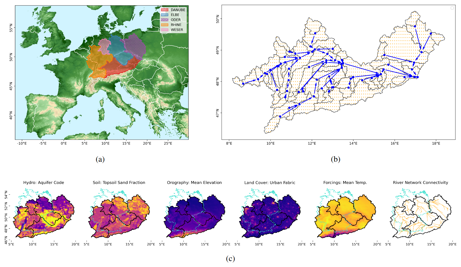
Figure 1 Overview of study area, input grid and data types. (a) Study Area: The study area comprises 5 basins that cover a contiguous area in central Europe. (b) Input Grid and Station Network in Upper Danube Basin: Cells of input grid (orange) for Upper Danube basin. Catchment boundaries (black) are overlaid with corresponding stations (blue), as well as connecting arrows representing the station connectivity network. Code to reproduce the river network is released together with this paper. (c) Input Types: Visualizations for one example feature of each type of input. Basin outlines (black) and borders of Germany (turquoise) are plotted for reference. Orography in panel (a) was adapted from the European Space Agency's Copernicus Global 90 m DEM (GLO-90, doi: https://doi.org/10.5270/ESA-c5d3d65, ESA, 2022) © EuroGeographics for the administrative boundaries in panel (a) and (c). Watershed boundaries in panels (a), (b), and (c) were taken from the Global Runoff Data Center (https://portal.grdc.bafg.de/applications/public.html, last access: 11 September 2025).

2.1 Meteorological Forcings

The meteorological forcings in our study were derived from the ERA5-Land dataset¹ (Muñoz Sabater, 2019; Copernicus Climate Change Service, 2022). Temporal aggregation from hourly to daily resolution was achieved differently for each variable: The temperature two meters above surface was aggregated by calculating minimum, mean and maximum values. Potential evapotranspiration was summed. Precipitation is provided in ERA5-Land as sub-daily values, meaning that the daily total sum corresponds to the value stored at 24:00. We added a measure of variability of precipitation by taking the variance over the increment at every hourly time step. Due to the good maintenance of the ERA5 dataset, there were no missing values in the temporal data, hence no interpolation was necessary on our part. Table A2 provides a detailed list of all dynamic variables.

2.2 Ancillary Data

Hydrogeological properties were derived from the International Hydrogeological Map of Europe (IHME)². The original dataset features six hydrogeological classes as well as two classes for snow-ice-fields and inland water bodies. The six classes represent the productivity of rock type, which indicates how easily water can dissipate through the bedrock. Classes are ordinal in that they are sorted by the corresponding productivity in ascending order. This allows us to take a non-rigorously defined but nonetheless informative average over the classes' proportions within each grid cell. We concatenate this productivity score with the binary categorical classes for snow-ice-fields and inland water bodies, each represented by a ratio of prevalence of this type of binary class within the grid cell.

Land Cover information was obtained from the Corine Land Cover Map³ (CLC). This dataset classifies land cover at three different levels of detail, with increasingly differentiated (sub)classes. We decided to use the second level, which containing 16 classes in total. Similarly to the procedure applied to the hydrogeological properties, we calculated a distributional vector representing the proportion of a given class covering the grid cell.

Soil type information was obtained from the dataset European Soil Database Derived Data⁴ (Hiederer, 2013a, b). This dataset features 17 different physical properties, separately for top soil and lower soil. We calculate the average value of each feature within a grid cell.

Orographic information was derived from the European Union Digital Elevation Map⁵ (EU-DEM). Elevation was averaged within each grid cell, as well as the gradient in latitudinal and longitudinal direction, and the steepness or magnitude of the two-dimensional gradient. This yielded a total of four orographic features.

Table A3 provides an detailed list of all ancillary variables in the same ordering as we just introduced, which is also the ordering in the data file.

2.3 Grid Harmonization

As a common grid format, we decided to use the grid of the ERA5-Land reanalysis dataset (Muñoz Sabater, 2019; Copernicus Climate Change Service, 2022), which covers the earth's surface with a 0.1°×0.1° resolution, corresponding to roughly 9 km × 9 km for the case of our study area. ERA5-Land contains a vast number of meteorological variables and has an hourly resolution, spanning from 1950 onward. It has been widely used and is actively maintained and updated. This means the dataset we provide with this paper remains easily extendable, should a user like to e.g. include an additional meteorological variable in their experiments, extend the study area or increase the temporal resolution. Our study area comprises a total of 7169 grid cells on this grid.

The spatial data originally comes in different formats (vector or grid), projections and resolutions. All data sources were thus harmonized to the grid of ERA5-Land. The first step consisted in converting the maps to a common coordinate system. For the sake of compatibility with ERA5, we decided to use the geographic coordinate system WGS 84. Then for each map separately, polygons covering 0.1° in latitude and longitude with the grid cell at the center were extracted. For categorical maps like hydrogeology and land cover, consisting of classes such as “Artificial surfaces: Urban fabric”, the fractions covered by each class within each polygon were calculated. This results in a distributional description of class occurrence maximally conserves the original information, as no averaging or other kind of aggregation is necessary. Quantitative information, like e.g. clay content in topsoil, was however aggregated in a final step within the polygon. As a downside to this approach, note that both cases require calculating coverage areas in a geographic coordinate system. This treats the surfaces as flat instead of accounting for the earth's curvature, making the calculations imprecise. We consider this effect negligible here since the surfaces contained in the grid cells are so small that they can be safely considered approximately flat. A more severe limitation is the fact that at high latitudes, polygons defined by a given latitudinal and longitudinal extent become substantially more narrow on the side facing the pole, which also impairs the calculation of area. We could not change the polygons to counteract this effect since they are implicitly dictated by the ERA5 grid. At the moderate latitudes of our study area and especially the small polygons used in the grid, this distortion can still be considered acceptable for the sake of harmonization with ERA5, depending on the application. However, applying this approach in polar regions for example would necessitate an intermediate step of choosing a suitable projected coordinate system for calculating the areas in order to make the distortion explicit and thus better understand its effects. Boundary effects are not an issue with this vector approach as no interpolation is required, however. All maps covered regions well exceeding the study area.

Specifically for the four map types, the hydrogeological map already came in the WGS 84 reference system. The land cover map came in vector format and LAEA coordinate system, so the polygon's coordinates could simply be calculated point-wise using the geopandas Python package (den Bossche et al., 2025) with pyproj (Snow et al., 2025) as a backend. This was followed by calculating the fraction of each class within the polygon described above. The soil map came in LAEA reference system but as a raster. We decided against interpolating as it would not contribute any additional information. Instead, we simply considered each cell in the raster as a separate polygon and calculated the fractions using the vector method described above. The situation was the same for the elevation map, with the added initial step of down-sampling the map from 25 m resolution to 500 m resolution using weighted average resampling implemented in rasterio (Mapbox, 2024).

3 Code and data availability

The dataset is available at https://doi.org/10.4211/hs.d7f2cbb587ab4a75ac7987854e8f62ca, (Vischer et al., 2025a). Dynamic meteorological forcing data and static ancillary data are stored in two separate NetCDF4 (Rew et al., 2006) files, “ancillary_pub.nc” and “dynamic_pub.nc”. This format allows for labeled coordinates such as latitude, longitude and date for convenient selection on spatial and temporal domains, respectively. All variables are named in a self-explanatory manner and we provide labeled metadata. See Tables A2 and A3 for a detailed reference of the included variables.

The data was processed in several Python Jupyter Notebooks (Granger and Pérez, 2021) that can be found in this repository: https://gitlab.hhi.fraunhofer.de/vischer/spatial_streamflow_dataprep, last access: 11 September 2025. The code requires Python 3.11 (Van Rossum and Drake, 2009) and is licensed under the Clear BSD licence. Additional dependencies are specified in an Anaconda environment (Anaconda, 2020) specification contained in the repository. The scripts are stand-alone and do not require further input parameters. Along with the code to process the data, we provide a script that loads the data, selects subsets and visualizes them. This can serve as a starting point for the user to interact with the data. Furthermore, we provide code to wrap all the data in a PyTorch (Ansel et al., 2024) Dataset class for further processing in a machine learning context. Since dense arrays are required for this, we provide an alternative format version of our features in the files “ancillary_paper.nc” and “dynamic_paper.nc”, where dimensions were transformed from latitude and longitude to a unique grid cell index. In this version, all features were standardnormalized in order to suit better the requirements of neural networks.

All data sources from which we obtained the original data have been widely used across various scientific fields for years, so we assume the original data to be valid. In order to technically validate our processing steps, we feature a testing script in our repository with extensive tests and visualizations of the compiled data. We also successfully employed this dataset in training a neural network model for rainfall streamflow modeling (Vischer et al., 2025b).

4 Conclusions

Combining a variety of data sources, we provide the first spatially resolved dataset for multivariate rainfall-streamflow modeling. It covers five entire river basins and it thus particularly suited for large-scale modeling of hydrological processes. With the publication of this dataset, we hope to stimulate further development of spatially resolved, high-resolution hydrological modeling beyond the scope of lumped catchments. Suitable for neural network models as well as conceptual and physical modeling approaches, we hope this dataset will facilitate model comparison and stimulate future development in the spatially resolved domain. Using the same spatial grid as ERA5 as well as daily resolution limits its expressiveness of small scale, e.g. convective events, where higher spatial and temporal resolution would be preferable. If users decide to spatially aggregate our data and want to use derived variables like hydrological or climate signatures as input for their models, they would have to manually compute them from the raw data contained in our dataset. This is especially the case for snow-related variables, as particularly the Southeast of our study area is dominated by snowmelt dynamics. Lastly, the dataset is of only limited use for training training models that are to be deployed world-wide. We focus on a contiguous area in central Europe, which means in turn that the dataset contains only a particular subset of all hydrological dynamics that can be observed.

Appendix A: Data Origins and Detailed List of Features

Muñoz Sabater (2019)Copernicus Climate Change Service (2022)Günther and Duscher (2019)Hiederer (2013a, b)

Table A1 Overview of source datasets and their authors for dynamic data/meteorological forcings contained in file forcings_pub.nc and static/ancillary data contained in ancillary_pub.nc. See Tables A2 and A3 for more details on derived features. Last access for all weblinks is 11 September 2025.

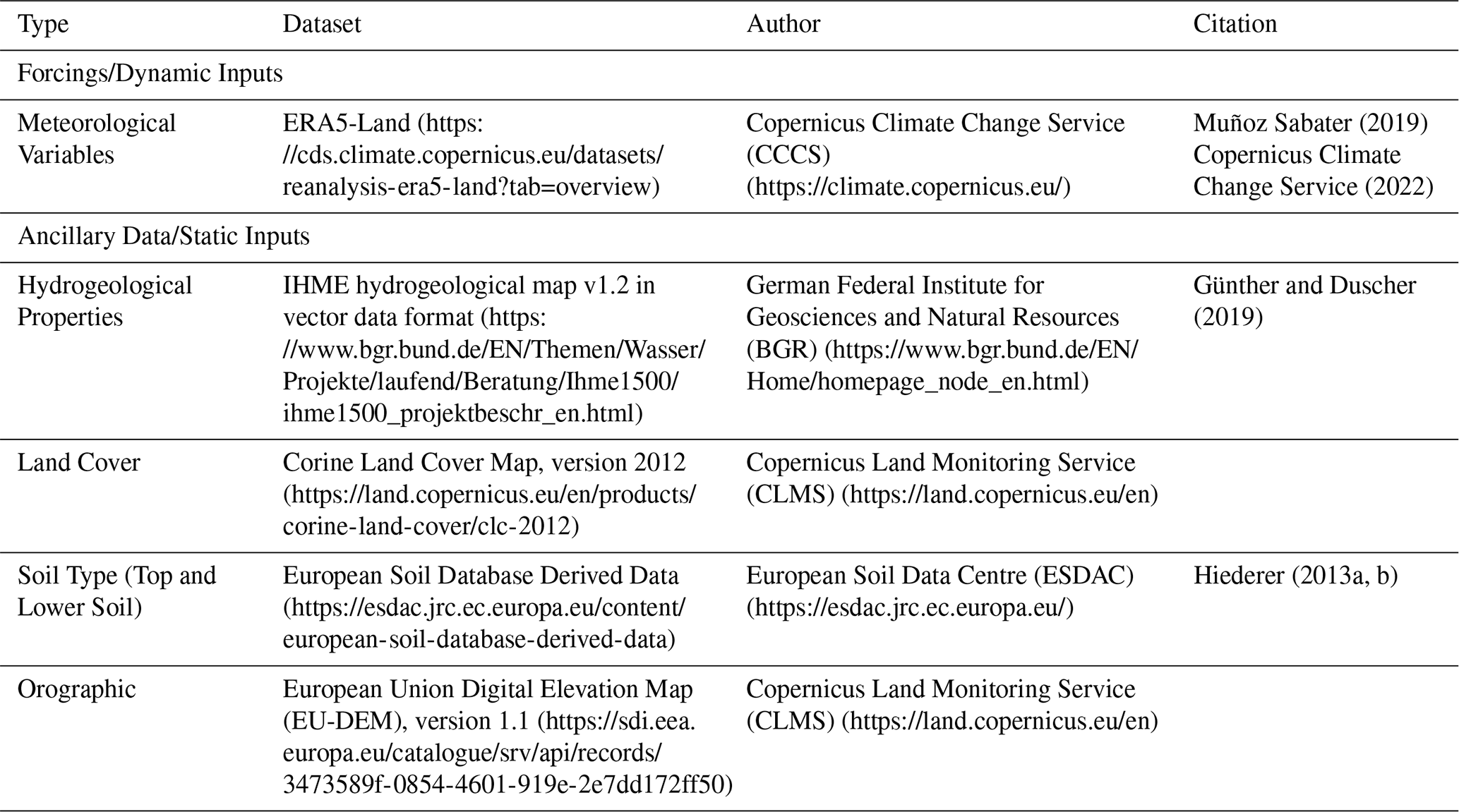
Table A2 Overview of dynamic input features in the file forcings_pub.nc. Empty cells indicate that the value is identical to the one above. Each of these features is a three-dimensional array with dimensions latitude, longitude and date. Labeled coordinate indices for all dimensions are contained in the file.

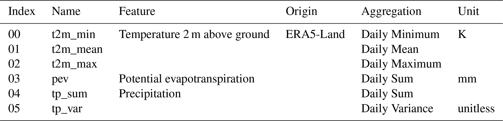
Table A3 Overview of static input features in the file ancillary_pub.nc. Empty cells indicate that the value is identical to the one above. Explanations of the features derived from Corine Land Cover map (CLC) and elevation map were omitted because the names are self-explanatory. Each of these features is a two-dimensional array with dimensions latitude and longitude. Labeled coordinate indices for all dimensions are contained in the file.

Appendix B: Comparison with Related Datasets

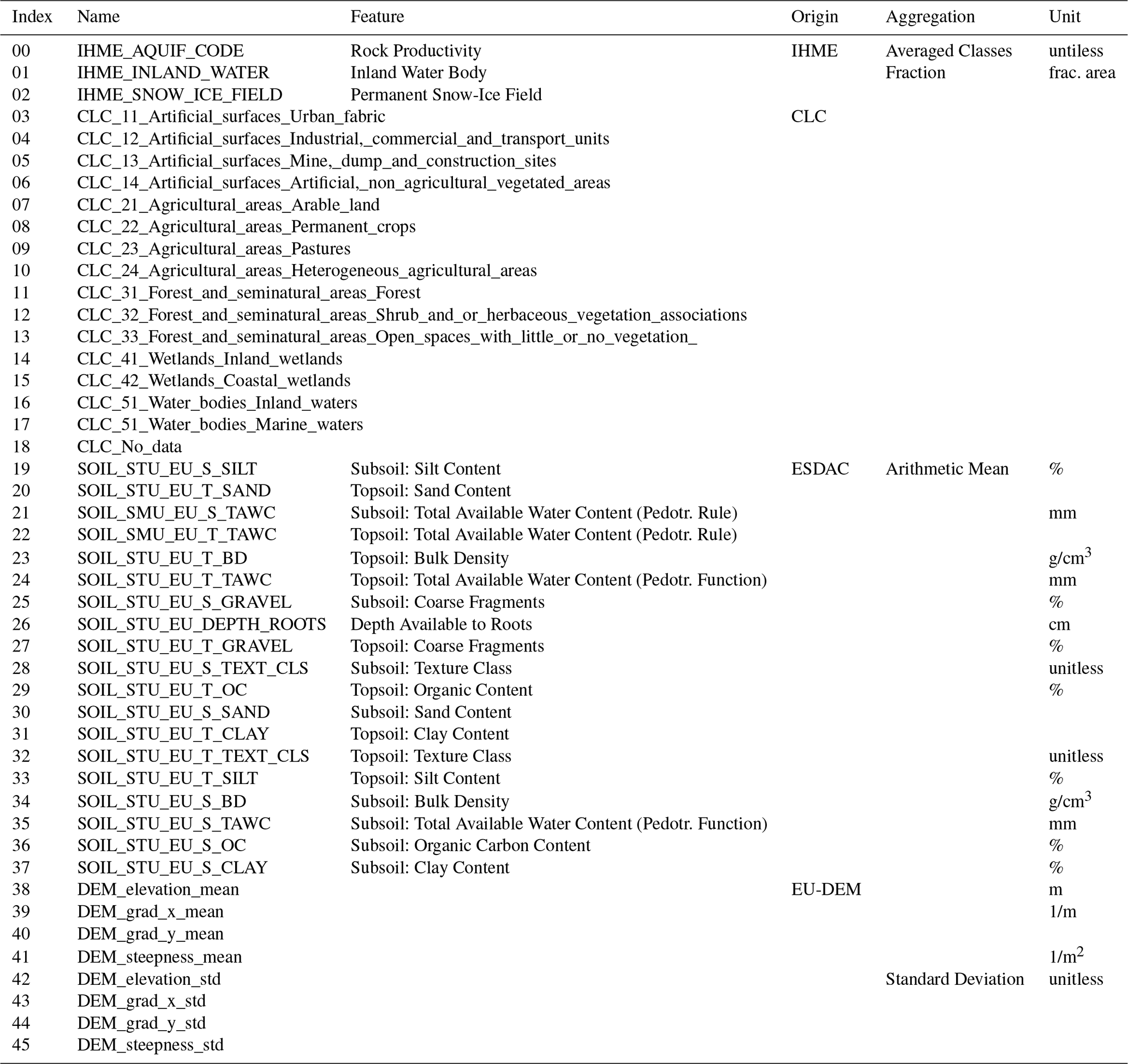
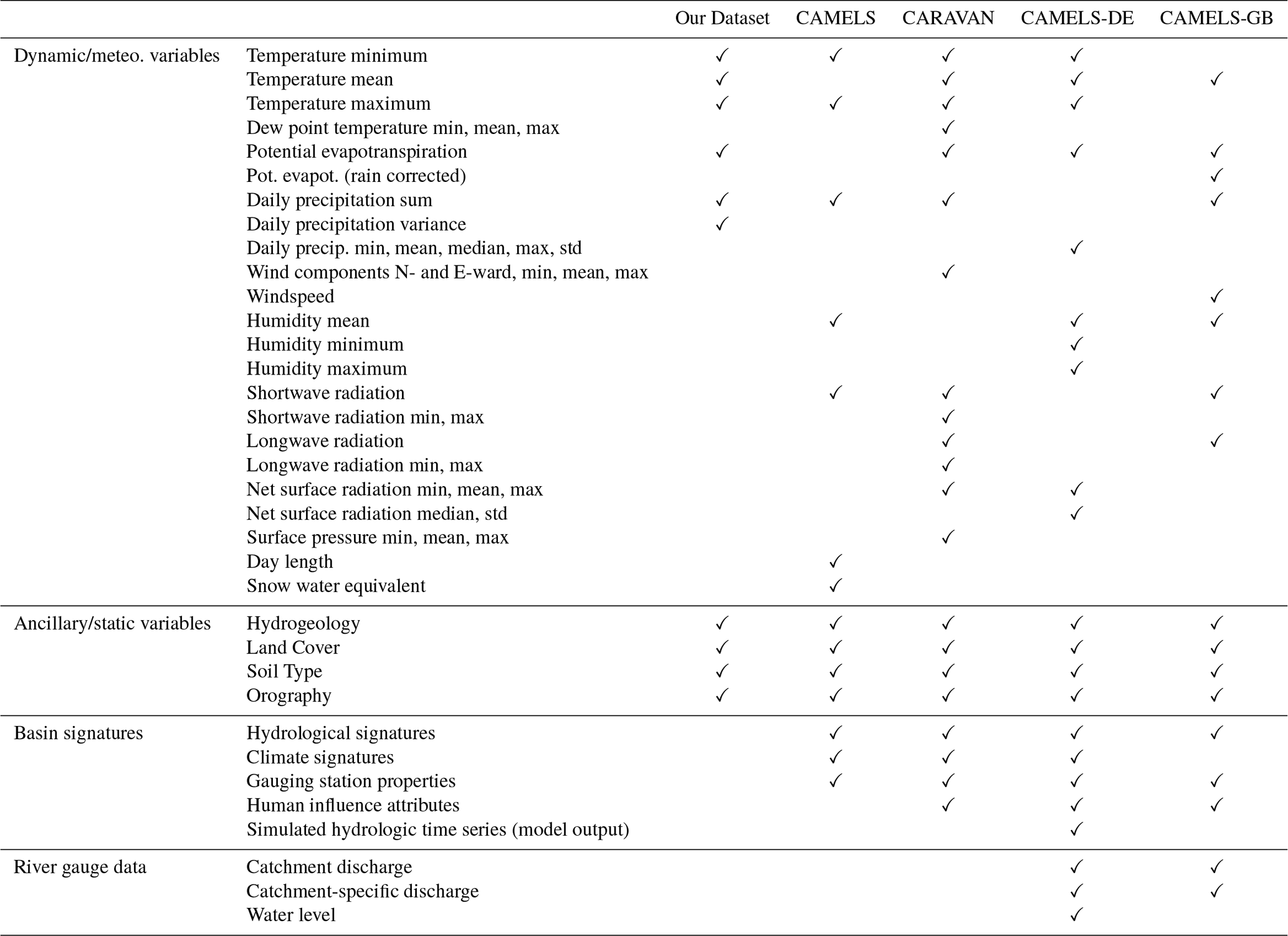
Table B1 This table compares the variables contained in our dataset to those contained in similar datasets. We matched the raw variables contained in the CAMELS dataset (Addor et al., 2017 and Newman et al., 2015) as precisely as data availability in our study area permits. This means that e.g. the classes for describing land cover type may vary, although the kind of information is the same. Our dataset also matches other established datasets in this domain rather closely in terms of selection of variables, namely CARAVAN (Kratzert et al., 2023), CAMELS-DE (Loritz et al., 2024) and CAMELS-GB (Coxon et al., 2020). The only substantial difference to all these datasets is that we opted not to include derived climate and hydrological signatures of basins, since any aggregation of our data is optional and would depend on the application. Arguably, since spatially resolved data is more abundant and detailed, it might render “summary statistics” of entire basins less relevant to begin with. In any case, signatures can be readily calculated from the raw data contained in our dataset according to the user's preference. Throughout the table, all listed temporal variables across all datasets are aggregated daily, so “mean” temperature refers to daily mean etc.