Global open-ocean daily turbulent heat flux dataset (1992–2020) from SSM/I via deep learning

Air–sea turbulent heat fluxes – latent heat flux (LHF) and sensible heat flux (SHF) – are fundamental to the Earth's energy and moisture budgets and to ocean–atmosphere coupling. Global flux estimates via bulk aerodynamic algorithms depend on sea surface temperature (SST), surface wind speed (SSW), near-surface air temperature (T_a), and specific humidity (Q_a), but orbital sampling and cloud contamination leave gaps in satellite inputs that propagate uncertainty to $T_{\mathrm{a}}/Q_{\mathrm{a}}$ and hence to LHF/SHF. Here we present DeepFlux, a global daily 1° × 1° heat-flux dataset for 29 years (January 1992–December 2020). The dataset is produced with a concise completion-then-retrieval workflow: Special Sensor Microwave/Imager (SSM/I) variables (SSW, cloud liquid water, total column water vapor, and rain rate) are first gap-filled using the AI-based Generalized Data Completion Model (GDCM) to yield spatiotemporally continuous inputs; these – together with Optimum Interpolation SST (OISST) – are then used to retrieve T_a and Q_a via the AI-based Matrices-Points Fusion Network (MPFNet). LHF and SHF are then computed using a bulk algorithm. Validation against in-situ buoy observations shows that the dataset closely matches the true measurements, with RMSEs of 0.53 °C (T_a), 0.70 g kg⁻¹ (Q_a), 5.53 W m⁻² (SHF), and 25.28 W m⁻² (LHF). Comparisons with widely used flux products indicate differences among products, reflecting variability in flux estimates from different sources. DeepFlux provides an open, consistent, observation-constrained view of near-surface meteorology and air–sea heat exchange for climate diagnostics, model evaluation, and process studies. DeepFlux v1.0 is openly available under CC BY 4.0 at https://doi.org/10.12157/IOCAS.20250823.001 (Wang et al., 2025b).

1 Introduction

Air–sea turbulent heat fluxes – latent heat flux (LHF) and sensible heat flux (SHF) – govern the exchange of energy and moisture at the air-sea interface and thereby influence weather, climate variability, and ocean circulation across scales (Andersson et al., 2010; Bentamy et al., 2013; Large and Pond, 1982; Trenberth et al., 2001). Variations in LHF and SHF modulate sea surface temperature (SST) and atmospheric conditions, with broad implications for diagnosing air–sea coupling and improving climate prediction (Cayan, 1992; Yu et al., 2004; Zhang and McPhaden, 1995; Bentamy et al., 2017; Zhou et al., 2019, 2020). High-quality, spatially and temporally continuous flux fields are therefore essential for process studies and model evaluation.

Flux estimates over the global ocean are typically derived from bulk aerodynamic formulations (e.g., the COARE family) that depend on input fields such as SST, near-surface wind speed (SSW), air temperature (T_a), and specific humidity (Q_a) (Fairall et al., 1996a, b, 2003; Large and Pond, 1982). In situ measurements provide accurate point observations but are sparse in space and time, being limited to research cruises and moored arrays such as TAO/TRITON (Bourlès et al., 2008; McPhaden et al., 1998). Satellites offer broad coverage but most passive sensors do not directly observe T_a and Q_a (Simonot and Gautier, 1989), prompting indirect approaches based on empirical relationships or statistical retrievals from satellite-derived variables (Wells and King-Hele, 1990; Liu, 1986; Schulz et al., 1997; Schlüssel et al., 1995; Jones et al., 1999). While such methods reduce typical flux errors to the order of 10–30 W m⁻², they remain sensitive to atmospheric regime, regional biases, and uncertainties in near-surface humidity and temperature (Berry and Kent, 2011).

Reanalysis and blended products integrate multiple observing systems and data assimilation to provide global fields of T_a, Q_a, and surface fluxes (Hersbach et al., 2023; Kalnay et al., 1996; Bentamy et al., 2003, 2013; Tomita and Kubota, 2006; Tomita et al., 2018; Schulz et al., 1997). These datasets are invaluable, yet spread among products persists – especially over data-poor basins – owing to differences in parameterizations, assimilation strategies, and input data quality (Bourassa et al., 2013; Esbensen et al., 1993; Meng et al., 2007). A persistent obstacle is the spatiotemporal incompleteness of satellite inputs, arising from orbital sampling and cloud contamination, which degrades the continuity of flux estimates and propagates uncertainties through the retrieval chain (Chou et al., 1995; Kubota et al., 2002; Schulz et al., 1997).

Recent advances in data-driven methods have shown promise in capturing nonlinear ocean–atmosphere relationships and improving geophysical retrievals (Wang et al., 2023, 2024; Wang and Li, 2023, 2024; Zhang and Li, 2024). To mitigate error propagation from missing inputs, we developed the Flux Model, which consists of two components: the Generalized Data Completion Model (GDCM) (Wang et al., 2025a) and the Matrices-Points Fusion Network (MPFNet) (Wang et al., 2025c). The Flux Model adopts an integrated “completion-then-retrieval” strategy: first constructing spatiotemporally continuous input fields to address data gaps using the previously developed GDCM (Wang et al., 2025a), and then performing the flux-related retrievals. In particular, we complete the key SSM/I variables – SSW, cloud liquid water (CLW), total column water vapor (WV), and rain rate (RR) – and account for the distinct diurnal signals associated with orbital sampling by processing ascending and descending passes separately before merging (Chou et al., 1995; Kubota et al., 2002; Schulz et al., 1997; Hollinger et al., 1990).

Using these completed inputs (together with SST), we retrieve T_a and Q_a with the MPFNet and compute SHF and LHF with a bulk algorithm, yielding a new daily flux dataset for the global open ocean at 1° × 1° resolution for 1992–2020 (hereafter DeepFlux. We evaluate DeepFlux against buoy observations and widely used benchmark products. Validation against buoy measurements indicates that DeepFlux aligns more closely with the buoy observations than the benchmark products in both $T_{\mathrm{a}}/Q_{\mathrm{a}}$ and fluxes, while comparisons among the benchmark products show differences between them (Bourlès et al., 2008; McPhaden et al., 1998; Bentamy et al., 2003, 2013). The dataset, code, and documentation are openly available (see Data/Code Availability).

This paper is structured as follows: Sect. 2 details the satellite, in situ, and reanalysis datasets used. Section 3 provides a detailed description of the DeepFlux products generated using the Flux Model, which is composed of two components: the GDCM for data completion and the MPFNet for inversion and bias correction. In Sect. 4, we rigorously validate DeepFlux against in situ observations and compare its performance with six state-of-the-art products. Section 5 discusses the spatiotemporal characteristics and long-term trends revealed by our dataset. Section 6 presents the code and data availability and Sect. 7 concludes the study.

2 Data and Processing

This section provides an overview of the data and preprocessing procedures used for data completion and model inversion. Satellite remote sensing products from the SSM/I sensor serve as the model's input. Missing dates in the satellite data are filled using interpolated ERA5 reanalysis data. In situ observations of T_a, Q_a, LHF, and SHF are used as ground-truth references. ERA5 data are also used for model pretraining and, along with NCEP, Institut Français de Recherche pour l'Exploitation de la Mer (IFREMER), Objectively Analyzed air-sea Fluxes (OAFlux), and Ocean Heat Fluxes Climate Data Record (OHF-CDR) products, for performance comparison.

2.1 Data and method

2.1.1 SSM/I data

The Special Sensor Microwave/Imager (SSM/I), flown on the Defense Meteorological Satellite Program (DMSP) series, is a conically scanning passive microwave radiometer designed to measure naturally emitted microwave radiation from Earth's surface and atmosphere. Since its initial deployment in 1987, SSM/I has provided synoptic, near-all-weather observations widely used for both operational weather applications and climate studies (Hollinger et al., 1990). The instrument carries seven frequency channels (19.35–85.5 GHz) that enable the retrieval of a variety of geophysical parameters. DMSP platforms follow near-polar orbits and typically provide two passes per day (ascending and descending), but the local equator-crossing time differs among satellites and drifts over mission life because the orbits are not maintained in strict local-time control (Wentz, 2013). In addition, multiple DMSP satellites often operate concurrently, increasing sampling but also introducing local-time heterogeneity in the long-term record (Fennig et al., 2020). Beginning in 2003, the Special Sensor Microwave Imager/Sounder (SSMIS) replaced SSM/I, adding sounding channels and extending high-frequency capabilities, thereby enhancing precipitation and cloud microphysical retrievals (Bommarito, 1993). Because of orbital geometry and conical scanning, swath gaps remain between adjacent passes, particularly in the tropics.

In this study, we use four key ocean atmosphere variables retrieved from the SSM/I to SSMIS series SSW, CLW, total column WV, and RR – together with SST from NOAA OISST v2.1 to retrieve global near-surface T_a and Q_a. Specifically, we use the Remote Sensing Systems (RSS) SSM/I to SSMIS Ocean Products (daily gridded fields; Version 7) for DMSP satellites F10-F17 over January 1992 December 2020 (RSS, 2026b; Wentz, 2013). RSS applies a unified physically based retrieval algorithm and Version-7 calibration/intercalibration to promote consistency across satellites and the SSM/I to SSMIS transition (Wentz, 2013; RSS, 2026b). We process ascending and descending passes separately and provide both pass-time-resolved daily fields in the final product.

Despite these processing efforts, certain data limitations remain. Swath gaps and rain contamination lead to missing or degraded retrievals in some regions and time periods, and local sampling times vary and drift across the DMSP constellation (Wentz, 2013; RSS, 2026a). To minimize local-time aliasing, we (1) treat ascending and descending branches separately throughout the gap-filling and retrieval procedures (Sect. 2.2) and (2) recommend using the mean of the two branches for long-term trend analyses (Sect. 5), while retaining each branch for studies focused on pass-time (diurnal sampling) characteristics.

2.1.2 OISST

The NOAA OISST dataset integrates observations from multiple platforms, including satellite infrared and microwave sensors, ship measurements, and buoy data. Using an optimal interpolation algorithm, it fills spatial gaps and merges data to produce daily global SST fields at a spatial resolution of 0.25° × 0.25°, covering the period from September 1981 to the present (Huang et al., 2021). In this study, we use global SST data from OISST v2.1 (1 January 1992 to 31 December 2020) along with GDCM-completed SSM/I SSW, CLW, WV, and RR data over the same period as input for the MPFNet model to retrieve global T_a and Q_a. Note that OISST is used as an auxiliary input to provide Ts because SSM/I does not directly retrieve Ts. Therefore, OISST is not used as a training target (“ground truth”) for MPFNet. MPFNet is first pretrained on the large-scale ERA5 dataset and then fine-tuned using satellite–in situ matchups, enabling adaptive adjustment of the input–output mapping and mitigating moderate systematic biases in externally sourced Ts. This design is consistent with our published MPFNet transfer experiments, in which using OISST as an alternative Ts input for SSM/I resulted in only minor performance degradation and still demonstrated robust adaptability for long-term SSM/I-series applications (Wang et al., 2025c).

2.1.3 In Situ Data

Continuous, systematic, and comprehensive in situ observations are essential for ocean climate research. In this study, we utilize three types of in situ datasets: the Global Tropical Moored Buoy Array (GTMBA), the coastal moored buoy network maintained by the National Data Buoy Center (NDBC), and version 3.0.2 of the ICOADS. Among them, the GTMBA and NDBC datasets are derived from buoy platforms, while ICOADS primarily contains ship-based observations.

The GTMBA is part of the Tropical Ocean Global Atmosphere (TOGA) program (Webster and Lukas, 1992). It aims to support research on seasonal to interannual climate variability in tropical regions through in situ buoy measurements. The NDBC, operated by the NOAA, is responsible for deploying and maintaining moored buoys and coastal meteorological stations across the U.S. coastal and offshore regions, providing long-term, high-quality meteorological and oceanographic observations. ICOADS is the world's most extensive and longest-running collection of surface marine observations, incorporating data from ships, buoys, and other platforms. Version 3.0.0 includes monthly updates from 1992 to 2014, while version 3.0.2 has provided near real-time monthly updates since 2015.

In this study, we select variables necessary for surface heat flux estimation from these three in situ sources, aligned temporally with SSM/I satellite observations from 1 January 1992 to 31 December 2020 (including SSW, CLW, WV, and RR), to construct a matched satellite–in situ dataset for further analysis.

2.1.4 Heat flux data products

In this study, we evaluate the T_a, Q_a, SHF, and LHF estimates from the DeepFlux dataset developed in this study against five widely recognized flux and reanalysis products – OHF-CDR, ERA5, NCEP, IFREMER v4.1, and OAFlux – which are extensively used in oceanic and climate research as reference datasets. Table 1 summarizes the characteristics of different heat fluxes products. These products serve as authoritative benchmarks for assessing the consistency and performance of DeepFlux. A brief description of each dataset is provided below.

Table 1 Table of characteristics of different heat flux products.

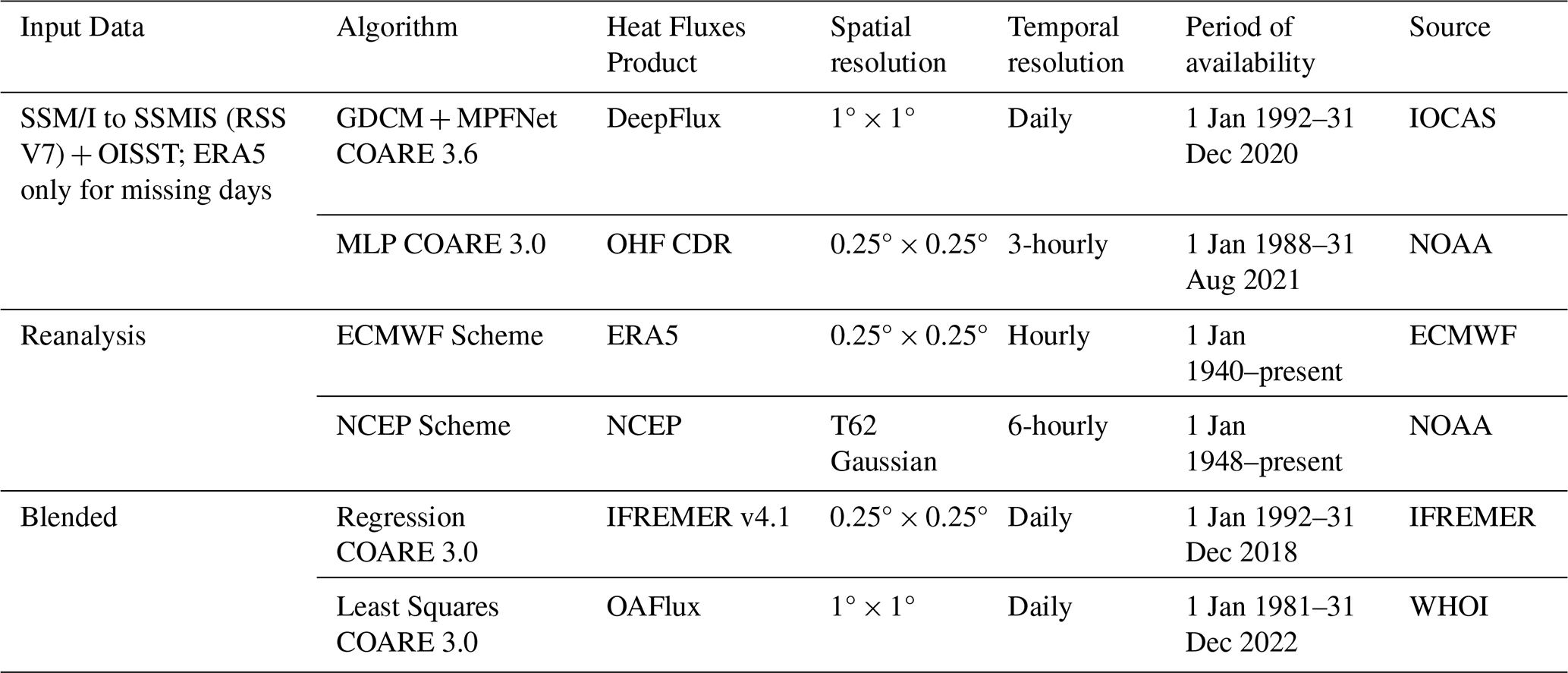
The OHF-CDR dataset is a long-term climate data record of global ocean heat fluxes and associated atmospheric parameters. It integrates passive microwave satellites (SSM/I, SSM/IS, AMSR), infrared sensors (AIRS, IASI), and reanalysis data (ERA5, MERRA-2), covering over 30 years since 1987, with a spatial resolution of 0.25° × 0.25° and a temporal resolution of 3 h. OHF-CDR estimates ocean-atmosphere heat fluxes using the COARE 3.0 algorithm. To compensate for the low sensitivity of microwave sensors near the surface, AIRS infrared data are introduced. Temperature is directly retrieved via radiative transfer equations from AIRS and fused with SSM/IS microwave data through a weighted nonlinear mapping between brightness temperature and atmospheric temperature. Deep learning is combined with physical modeling to derive initial TPW and specific humidity vertical profiles using SSM/IS and AIRS data along with SST and SSW. These initial fields are refined via a 1D variational assimilation constrained by radiative transfer, resulting in a gridded 0.25° product. This dataset provides reliable humidity fields for studies on ocean-atmosphere energy exchanges (Clayson and Brown, 2016; Roberts et al., 2010).

ERA5, developed by the ECMWF, is one of the core global high-resolution atmospheric reanalysis products. It provides hourly global ocean-atmosphere variable data with a spatial resolution of 0.25°, covering the period from 1950 to the present with continuous updates. ERA5 integrates multi-source observations – including satellite remote sensing, surface weather stations, and ocean buoys – through a four-dimensional variational assimilation system (4D-Var), enabling accurate and temporally continuous representations of ocean-atmosphere variables. It serves as an authoritative data source for related research (Hersbach et al., 2023; Hersbach et al., 2020).

The NCEP reanalysis datasets were developed jointly by the NCEP and the NCAR. They include two generations: NCEP/NCAR Reanalysis 1 (from 1948 to present) and NCEP-DOE Reanalysis 2 (from 1979 to present). These datasets provide global ocean-atmosphere parameters with a temporal resolution of 6 h and a spatial resolution of approximately 2.5°. NCEP reanalysis uses 3D-Var assimilation to integrate multi-source observations from ships, buoys, and satellite remote sensing. It is based on the Global Spectral Model (GSM) to dynamically simulate fields such as SSW, temperature, and humidity (Kalnay et al., 1996).

IFREMER v4.1, developed by the French Research Institute for Exploitation of the Sea (IFREMER) in collaboration with the European Space Agency (ESA) and climate research institutions, is one of the leading satellite-based ocean-atmosphere flux products. It calculates air-sea fluxes using the COARE 4.0 algorithm and provides global flux data with a daily temporal resolution and 0.25° spatial resolution. Covering the full span of multiple satellite missions, the dataset extends from 1993 to the present (Fairall et al., 2003).

The OAFlux air-sea flux dataset, developed by the Woods Hole Oceanographic Institution (WHOI), spans from 1958 to the present, with a spatial resolution of 1° and both daily and monthly temporal resolutions. OAFlux integrates multi-source data, including satellite observations, reanalysis products, and in situ measurements. Sea surface temperature is derived from blended satellite products such as AVHRR (infrared) and AMSR-E (microwave) data, while atmospheric temperature and humidity are primarily based on ERA-Interim and MERRA-2 reanalyses, corrected using satellite-retrieved specific humidity from SSM/I and AMSR-E. Surface turbulent heat fluxes are estimated using the COARE 3.0 algorithm, incorporating SSW data from satellite scatterometers (QuikSCAT, ASCAT). The uncertainties in latent and sensible heat fluxes are constrained within ±10 and ± 5 W m⁻², respectively, making OAFlux a reliable dataset for long-term climate studies and air-sea interaction analysis (Chou et al., 2003; Yu, 2008).

2.2 Data processing

2.2.1 Overall flow of data processing

Our data processing workflow is a comprehensive pipeline designed to first create complete input fields and then apply a novel two-stage inversion and correction scheme to produce the final heat flux dataset. The initial inputs for our model are remote sensing data from SSM/I – specifically SSW, CLW, WV, and RR – which are combined with the OISST dataset. Given the distinct diurnal variations associated with the satellite's northbound and southbound orbits, all SSM/I data are divided into ascending and descending orbit datasets for separate processing. Since the raw SSM/I data contain significant gaps due to orbital mechanics, we first apply the GDCM (Wang et al., 2025a) model to perform data completion, resulting in two complete sets of spatiotemporally continuous remote sensing observations.

Once the input data fields are complete, the retrieval process commences using the MPFNet architecture (Wang et al., 2025c). The first step is the primary retrieval of T_a and Q_a. To address the sample imbalance inherent in the matched satellite-in situ dataset, the MPFNet model is first pretrained on ERA5 data, then fine-tuned using a training set constructed from matched remote sensing and in situ observations. Because OISST provides Ts as an external predictor, we rely on the ERA5 pretraining + matchup fine-tuning strategy to adapt the input–output mapping and reduce sensitivity to moderate systematic biases in the Ts input, as demonstrated in our published MPFNet transfer experiments (Wang et al., 2025c). This process yields initial global T_a and Q_a fields, from which preliminary LHF and SHF are calculated using the bulk aerodynamic formulas (Eqs. 1 and 2).

Because the completion and retrieval stages are machine-learning based, specific model design choices (e.g., temporal length and incremental-learning strategy for GDCM; predictor selection, matrix size, and architectural/training techniques such as ERA5 pretraining and transfer learning for MPFNet, Pan and Yang, 2010) can affect the results. In generating DeepFlux, we adopt the peer-reviewed configurations of GDCM and MPFNet that have been evaluated through sensitivity/ablation experiments, and we summarize the key ablation evidence in the Supplement (Figs. S4–S7); full details are provided in the companion methodology papers (Wang et al., 2025a, c).

However, a critical challenge emerged from the input data itself. Our analysis revealed significant errors in the SSM/I SSW data when compared against in situ observations (as shown in Fig. S3). To mitigate the impact of this and other input uncertainties on the final fluxes, we implemented a second-stage correction model. This model, also based on the MPFNet architecture, is specifically designed to correct for systematic biases. It takes the initially retrieved LHF and SHF, along with all their constituent variables (T_a, Q_a, SST, Q_s, and SSW), as inputs. By training on the discrepancies between these preliminary fluxes and in-situ-derived fluxes, the model learns to correct for biases, particularly those originating from SSW inaccuracies. The final, bias-corrected LHF and SHF from this second stage constitute our DeepFlux dataset. This entire multi-step data processing workflow is illustrated in Fig. 1.

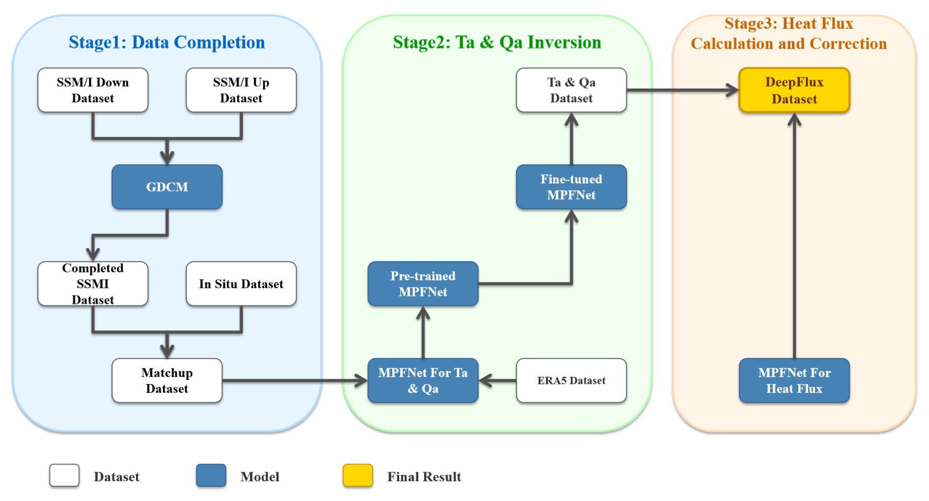
Figure 1 Data Processing Flowchart. The left panel illustrates the data completion stage, where SSM/I variables are gap-filled using GDCM to generate continuous inputs. The middle panel represents the stage of applying MPFNet to retrieve T_a and Q_a. The right panel shows the heat flux calculation and correction stage, where the final DeepFlux dataset is produced.

2.2.2 Data processing in the data-completion phase

In this study, the GDCM model is trained using complete ERA5 data, and the spatial resolution of the data was 1° × 1° (60° S–60° N, 0–360°). To simulate the missing patterns in SSM/I, a binary mask is created with the same spatial distribution, values of 1 indicating valid data and 0 indicating missing data. This binary mask is multiplied by the ERA5 data to generate simulated remote sensing data with missing values. A sliding window approach is then applied to format the data for GDCM input, using a 7 d window with a stride of 1 d. The complete ERA5 data from the 7th day serves as the ground truth, forming the training dataset for the GDCM model.

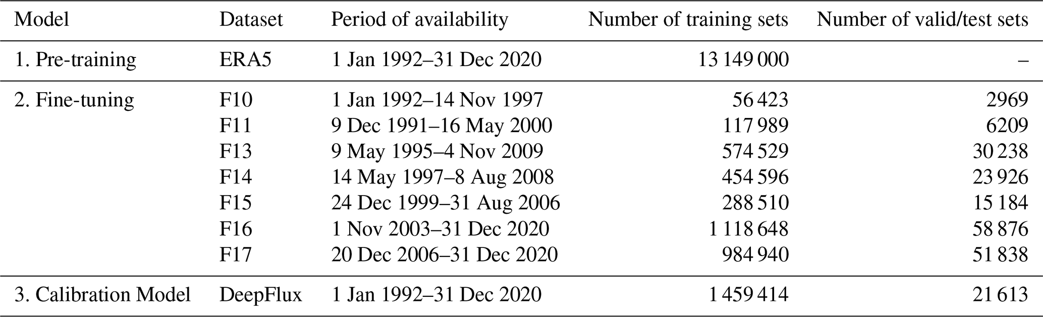
In the first step, ERA5 data served as both the input and output for the pre-training phase, which adjusted the randomly initialized MPFNet to produce the pre-trained MPFNet. One thousand random points were sampled daily (at 00:00) from the ERA5-provided T_a and Q_a as label data to pre-train the inversion model (MPFNet), covering the period from 1 January 1992 to 31 December 2020 (excluding 2018), with a total of 13 149 000 records. In the second step, data from SSM/I F10–F16 satellites matched with buoy observations (excluding WHOTS/Stratus/NTAS, which are reserved for independent evaluation) are used to fine-tune the MPFNet model, with 5 % of the data (excluding 2018) randomly selected as the validation set for each model. Due to the earlier observation periods of F10 and F11, fewer matched records with buoy data are available, leading to overfitting during training. To address this issue, we combine F15 and F17 data – which do not overlap in time with F10 and F11 – with the earlier records to mitigate overfitting during fine-tuning. In the final step, the calibration model's training set includes observed data from 1992 to 2020, excluding 2018, with 1 459 414 matched records. Data from 2018 are used as the test set, with 21 613 matched records. The detailed split of the training and test sets is shown in Table 2.

Table 2 Table of training/test set data details.

2.2.3 Calculation of heat flux

LHF and SHF are calculated using the COARE bulk air–sea flux algorithm (Fairall et al., 2003), here implemented using COARE version 3.6 (COARE3.6, 2017). The algorithm takes bulk inputs including SST, near surface air temperature (T_a), near-surface specific humidity (Q_a), and wind speed (SSW), and computes turbulent transfer coefficients iteratively as functions of atmospheric stability, sea-state-dependent roughness lengths, and Monin Obukhov similarity theory (Fairall et al., 2003; COARE3.6, 2017). In our implementation, T_a and Q_a are provided on the model grid (Sect. 2.2.2), SST is from OISST, and SSW is from the completed RSS SSM/I to SSMIS fields. The basic formulation is as follows:

$$\begin{array}{}\text{(1)}& {\displaystyle }\mathrm{SHF}=\mathit{\rho }{c}_{\mathrm{p}}{c}_{\mathrm{h}}U\left(T_{\mathrm{s}}-T_{\mathrm{a}}\right)\text{(2)}& {\displaystyle }\mathrm{LHF}=\mathit{\rho }{L}_{\mathrm{e}}{c}_{\mathrm{e}}U\left(Q_{\mathrm{s}}-Q_{\mathrm{a}}\right)\end{array}$$

Here, ρ denotes air density, c_p is the specific heat capacity of air, c_h is the turbulent heat exchange coefficient, U represents SSW, L_e is the latent heat of evaporation, and c_e is the turbulent moisture exchange coefficient.

2.2.4 Matchup Data

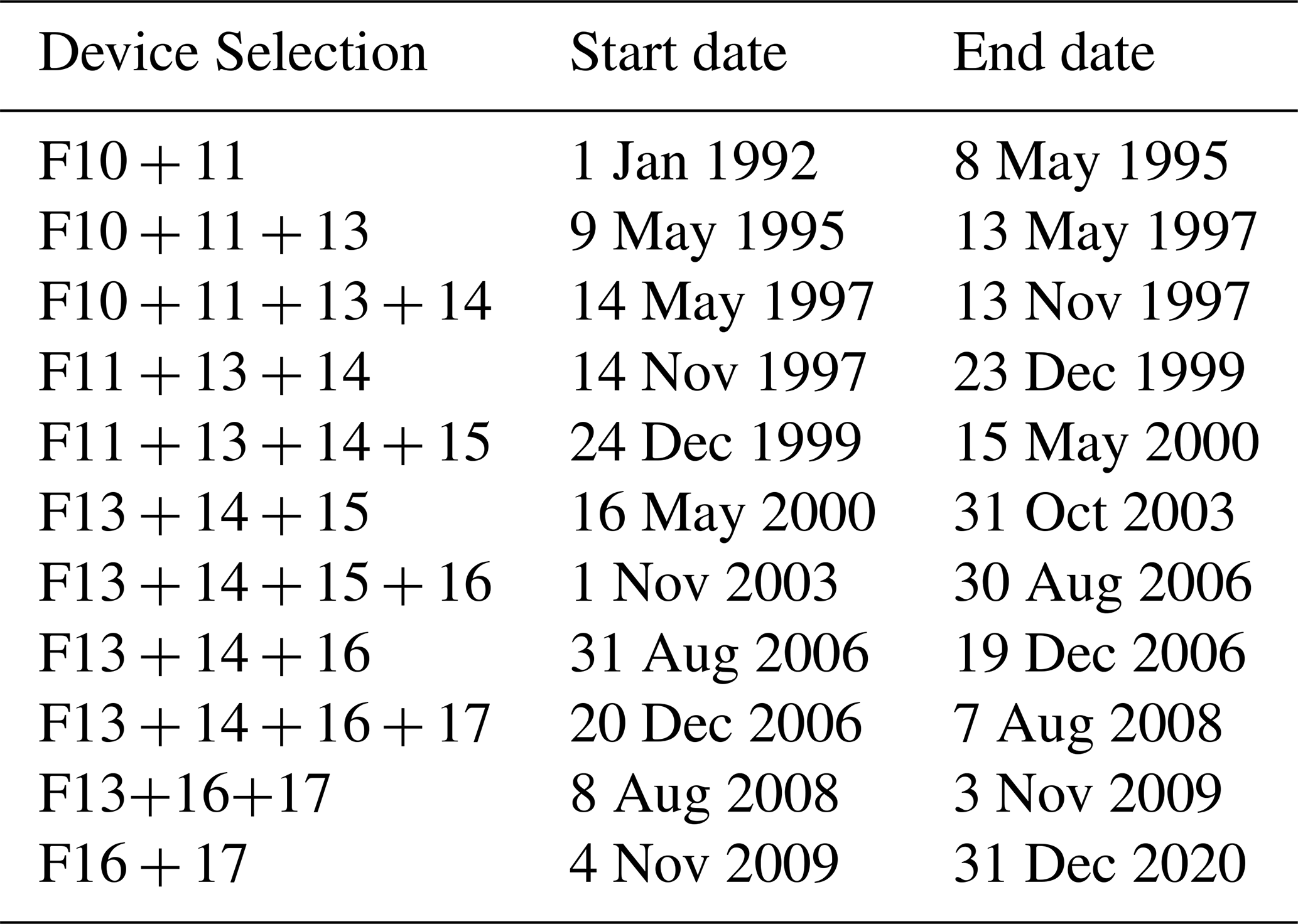
Matchup data, which pair satellite retrievals with coincident in situ measurements, are essential for calibrating retrieval algorithms and evaluating data quality. As shown in Table 1 in the second step, Fine-tuning, it is necessary to match SSM/I satellite data with in situ observations in order to retrieve T_a and Q_a. In this study, we use variables retrieved from the SSM/I satellite, including SSW, CLW, WV, and RR. All satellite data are divided into ascending and descending passes, corresponding to the satellite's northbound and southbound orbits, respectively. We utilize data from DMSP satellites F10 to F17, which have overlapping operational periods. Because overlapping DMSP satellites may sample different local times, their concurrent observations can reflect not only sensor differences but also real sub daily variability. This temporal overlap allows for observations from multiple satellites at the same time, as shown in Table 2, thereby increasing data redundancy. For periods with duplicate satellite data, we select the record with the lowest RMSE compared to in situ measurements as the final entry. In cases where in situ data are not available for comparison, the data from the newest When in situ data are unavailable for comparison, data from the most recent satellite are retained. This ensures each satellite observation corresponds to one ground-truth measurement. Additionally, 220 d of missing observations are filled using interpolated ERA5 reanalysis data at a 1° spatial resolution (Table S1 in the Supplement). The final satellite dataset spans 28 years, as detailed in Table 1 of the final step in the Calibration Model. The specific time coverage for each satellite is detailed in Table 3.

Table 3 Table of satellite data time ranges.

3 DeepFlux Products

The DeepFlux is generated based on the Flux Model, which first applies the GDCM to fill observational gaps, and then uses the MPFNet to retrieve air–sea heat flux variables. In this study, we used the GDCM data completion model developed by Wang et al. (2025a) and the MPFNet model developed by Wang et al. (2025c) to retrieve ocean surface heat fluxes. The GDCM model integrates the strengths of Convolutional Long Short-Term Memory (ConvLSTM) networks and attention mechanisms to complete missing data by leveraging spatiotemporal information. ConvLSTM captures spatiotemporal features of the data, while the attention mechanism (Vaswani et al., 2017) enables the model to dynamically focus on key information by assigning weights to emphasize important features and suppress redundant ones, making it especially effective for handling temporal dependency tasks. Figure S1 illustrates the overall architecture of the GDCM model. The GDCM framework consists of four main components: a spatiotemporal feature extraction block, a spatiotemporal motion extraction block, a multi-source spatiotemporal attention selection block, and an ASPP module. Detailed descriptions of each component are provided in the Supplementary Materials.

The GDCM-completed SSM/I data, combined with OISST, are used as inputs to the MPFNet model to retrieve T_a and Q_a. MPFNet is a satellite-to-surface parameter retrieval model based on an encoder-decoder architecture, as shown in Fig. S2. The model consists of five main components: the input module integrates five satellite observation variables – SSW, CLW, WV, RR (all completed by the GDCM model), SST (OISST) – and their corresponding latitude and longitude information; the matrix encoding module extracts spatial distribution patterns of satellite remote sensing images using FNO and analyzes environmental features at multiple scales through downsampling; the point encoding module employs ResNet to capture spatiotemporal variation patterns from historical observations at target locations; the feature fusion module combines global spatial features and local point features through residual connections; and the output module generates the predicted values of atmospheric temperature and humidity. By using a parallel encoding architecture and a multi-scale feature fusion strategy, MPFNet effectively addresses the limitations of traditional methods in modeling global-local features, improving the accuracy of T_a and Q_a retrieval. Detailed descriptions of each module are provided in the Supplementary Materials.

4 Results validation and discussion

In this section, we conduct a comprehensive evaluation of the SSM/I-derived heat flux dataset against buoy measurements and show that it is closer to the buoy observations than other mainstream heat flux products. The in situ and satellite matchup dataset from the test set, consisting of 21 613 records from 2018, was used to evaluate the performance of our DeepFlux and other products.

4.1 Comparison of statistical indicators for different heat flux products

In this section, we compare the performance of the SSM/I heat flux dataset with similar datasets from NCEP, ERA5, CDR, IFREMER, and OAFlux. Unlike existing heat flux products such as OAFlux, IFREMER, and ERA5, which are primarily reanalysis- or synthesis-based and often subject to spatial or temporal discontinuities, DeepFlux provides the first satellite-based, globally seamless, daily ocean surface heat flux dataset derived primarily from the SSM/I to SSMIS series (with OISST SST and limited ERA5 infill for missing days) using advanced AI-driven models. This design ensures improved temporal resolution, observational fidelity, and consistency across the 1992–2020 record, making DeepFlux a valuable complement to reanalysis and blended datasets.Correlation Coefficient (CC) and RMSE are used as evaluation metrics to assess the quality of each product comprehensively. In the SSM/I dataset, T_a and Q_a are divided into ascending and descending orbit datasets, which are trained and evaluated separately.

Figure 2 presents Taylor diagrams and Fig. 3 presents scatter plots comparing various heat flux products with in situ observations, while Table 4 summarizes their performance in terms of RMSE and CC. Among all datasets evaluated, the SSM/I heat flux product shows the highest accuracy and consistency with in situ data, achieving the lowest RMSE and highest CC for T_a, Q_a, SHF, and LHF (Fig. 2).

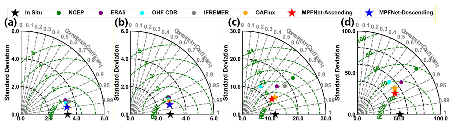
Figure 2 Taylor diagrams comparing NCEP, ERA5, OHF CDR, IFREMER, OAFlux, MPFNet-Ascending, and MPFNet-Descending with in situ observations for (a) T_a, (b) Q_a, (c) SHF, and (d) LHF. The radial distance represents the standard deviation (SD), the azimuthal angle represents the correlation coefficient (CC), and the green dashed contours indicate the centered root-mean-square error (RMSE). In situ observations are denoted by the black star; NCEP, ERA5, OHF CDR, IFREMER, and OAFlux are shown by colored circles; and MPFNet-Ascending and MPFNet-Descending are shown by the red and blue stars, respectively.

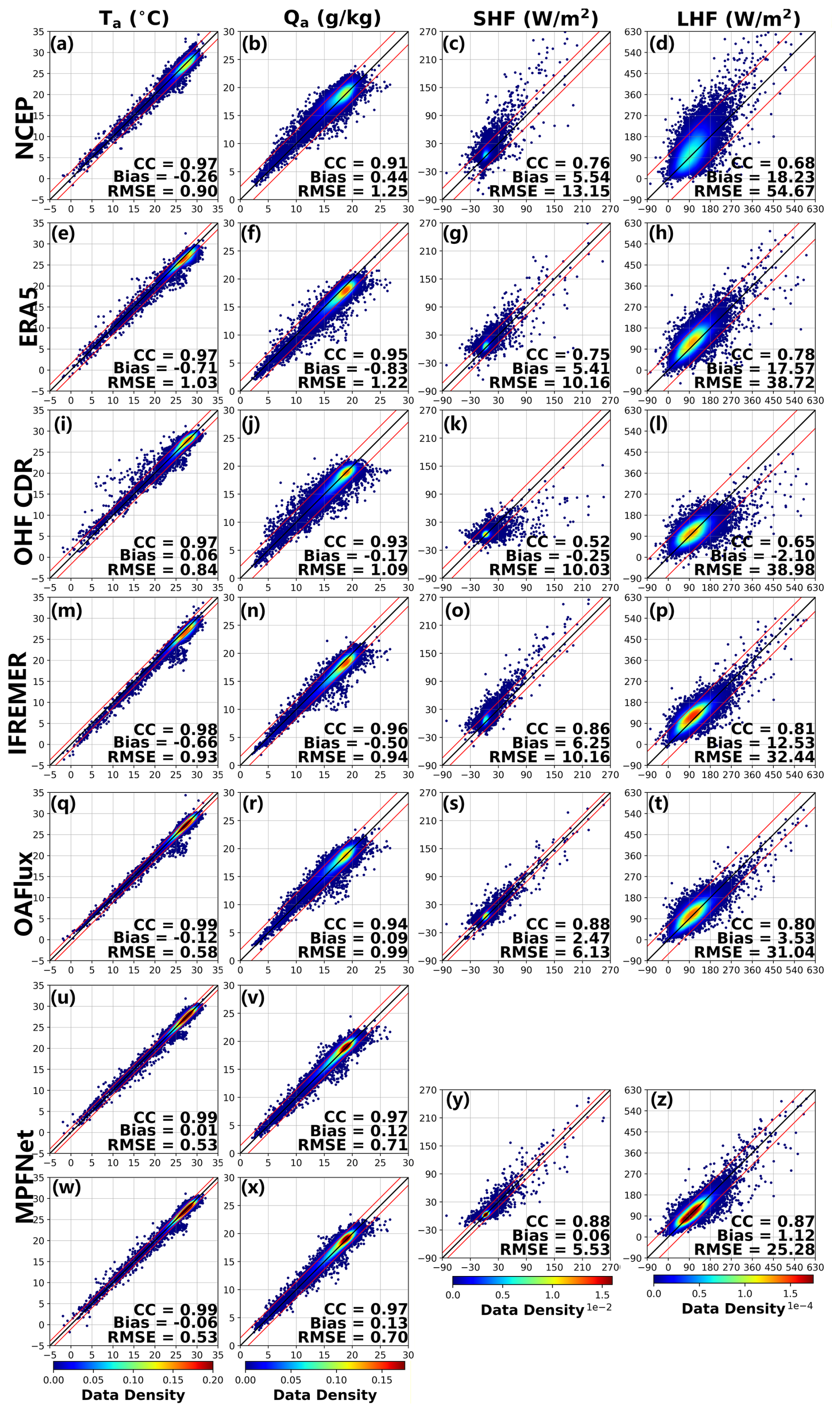
Figure 3 Scatterplots of T_a, Q_a, SHF, and LHF retrieved from different products against in situ observations. Panels (a)–(d), (e)–(h), (i)–(l), (m)–(p), and (q)–(t) correspond to NCEP, ERA5, OHF CDR, IFREMER, and OAFlux, respectively, for T_a (first column), Q_a (second column), SHF (third column), and LHF (fourth column). Panels (u)–(v) and (w)–(x) show the MPFNet results for T_a and Q_a from the two orbital branches (ascending and descending, respectively), while panels (y)–(z) show the MPFNet estimates of SHF and LHF. The black line denotes the 1:1 reference line, and the two red lines indicate the ±2 standard-deviation envelope of the retrieval–observation differences, encompassing approximately 95 % of the samples. Color shading indicates data density, and the CC, Bias, and RMSE values are given in each panel.

To specifically assess the effectiveness of the GDCM infilling, we provide supplementary diagnostics that compare errors in data-missing versus non-missing regions (see Figs. S4–S5 and Tables S1–S2), based on the completion-validation framework reported in the companion GDCM paper (Wang et al., 2025a).

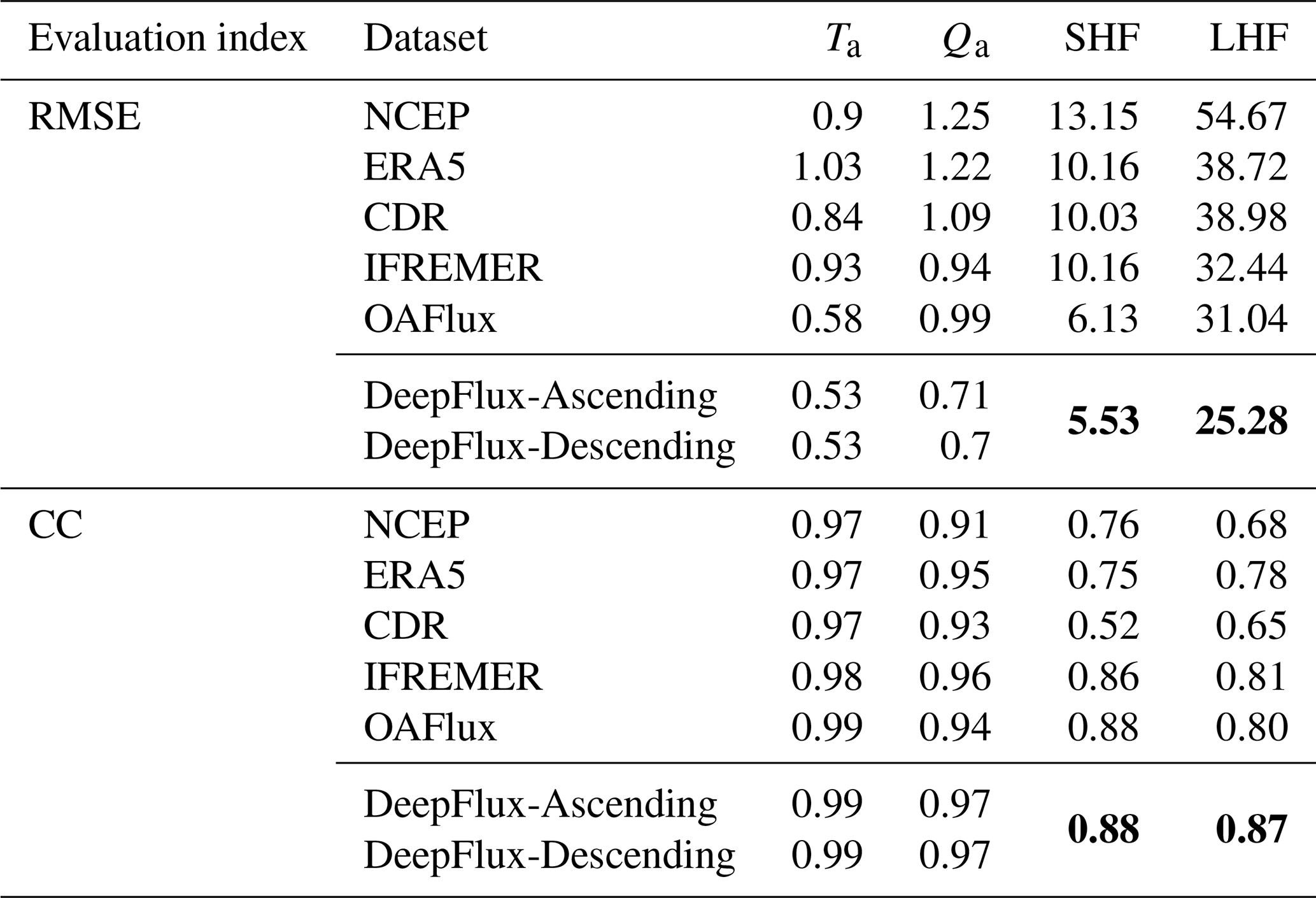
Specifically, for T_a, the SSM/I RMSE is 0.53 °C compared to ERA5's 1.03 °C, representing a 48.54 % improvement in accuracy. For Q_a, the SSM/I RMSE is 0.70 g kg⁻¹ versus 1.25 g kg⁻¹ for NCEP, a 44 % gain. For SHF and LHF, SSM/I achieves RMSEs of 5.53 and 25.28 W m⁻², respectively, compared to NCEP's 13.15 and 54.67 W m⁻², improving accuracy by 57.95 % and 53.76 % (Fig. 3, Table 4). These results further highlight the reliability and high quality of the SSM/I heat flux dataset.

Table 4 Evaluation Metrics of Seven Datasets Across Four Heat Flux Variables. Bold values indicate the best-performing dataset for a given metric/variable combination (lowest RMSE and highest CC${/}^{\mathrm{2}}$, as applicable).

4.2 Comparison of monthly average time series of independent validation datasets

To facilitate regional analysis and evaluation, we selected monthly averaged data from three independent buoy stations – NTAS (51° W, 15° N), Stratus (85° W, 22° S), and WHOTS (158° W, 22.7° N) – as additional datasets to assess the accuracy of different heat flux products under varying environmental conditions. To ensure independence, observations from these three moorings are withheld from model training and used only for independent evaluation. The time spans covered are 2002–2020, 2001–2020, and 2005–2020, respectively, as shown in Figs. 4–7.

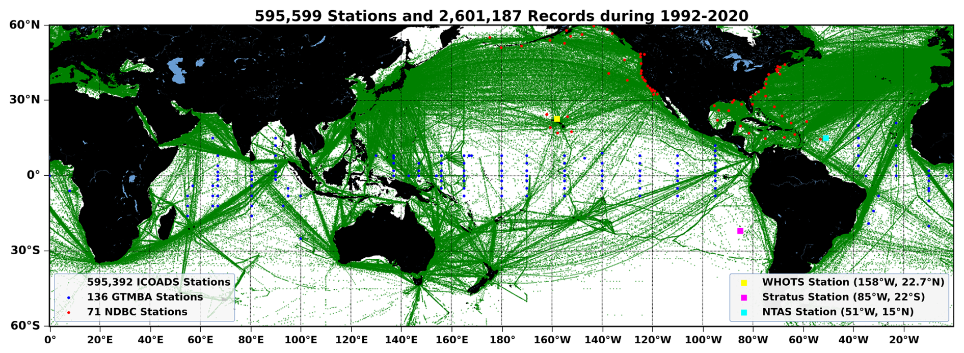
Figure 4 Spatial distribution of the 71 NDBC, 136 GTMBA, and 595 392 ICOADS stations matched with SSM/I during 1992–2020, yielding a total of 2 601 187 satellite–in situ matchup records. The independent validation stations used in this study are highlighted by colored squares: WHOTS (158° W, 22.7° N; yellow), Stratus (85° W, 22° S; magenta), and NTAS (51° W, 15° N; cyan).

The three selected independent buoy stations are located in the central Pacific, southeastern Pacific, and Atlantic Ocean, respectively. Oveall, in terms of long-term trends, the SSM/I-based heat flux dataset demonstrates strong consistency with in situ observations across all stations, while the NCEP product shows varying degrees of bias depending on location. Specifically, at the WHOTS Station in the tropical Pacific, where the monthly mean T_a exceeds 21 °C, the SSM/I dataset achieves the lowest RMSE for T_a (0.40 and 0.41 °C). Its RMSEs for monthly mean SHF and LHF are 3.93 and 15.2 W m⁻², respectively, while the other five mainstream datasets show SHF and LHF RMSEs above 7 and 19 W m⁻². The SSM/I ascending-track Q_a data has the lowest RMSE at 0.61 g kg⁻¹, and the descending-track RMSE is slightly lower than ERA5 at 0.69 g kg⁻¹ (Fig. 5).

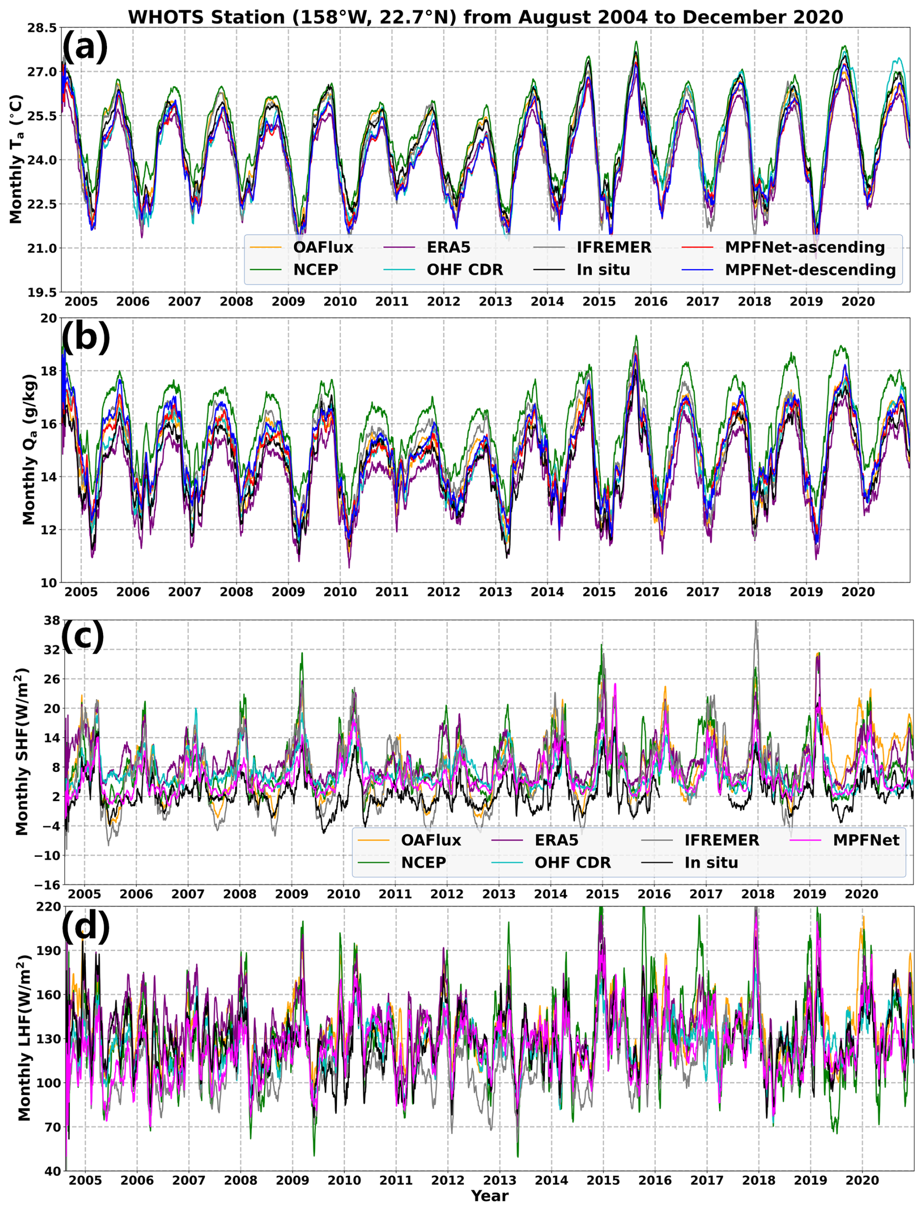
Figure 5 Monthly time series comparison at the WHOTS station (158° W, 22.7° N) from August 2004 to December 2020. Panels (a)–(d) show T_a, Q_a, SHF, and LHF, respectively. OAFlux, NCEP, ERA5, OHF CDR, IFREMER, and MPFNet retrievals are compared with in situ observations. For T_a and Q_a, the MPFNet ascending and descending retrievals are shown separately, whereas for SHF and LHF the MPFNet estimates are shown as a single series.

At the Stratus Station in the southeastern Pacific, SSM/I achieves the lowest monthly mean RMSEs across all variables, with Q_a ascending and descending RMSEs slightly higher than IFREMER at 0.71 and 0.65 g kg⁻¹, respectively (Fig. 6).

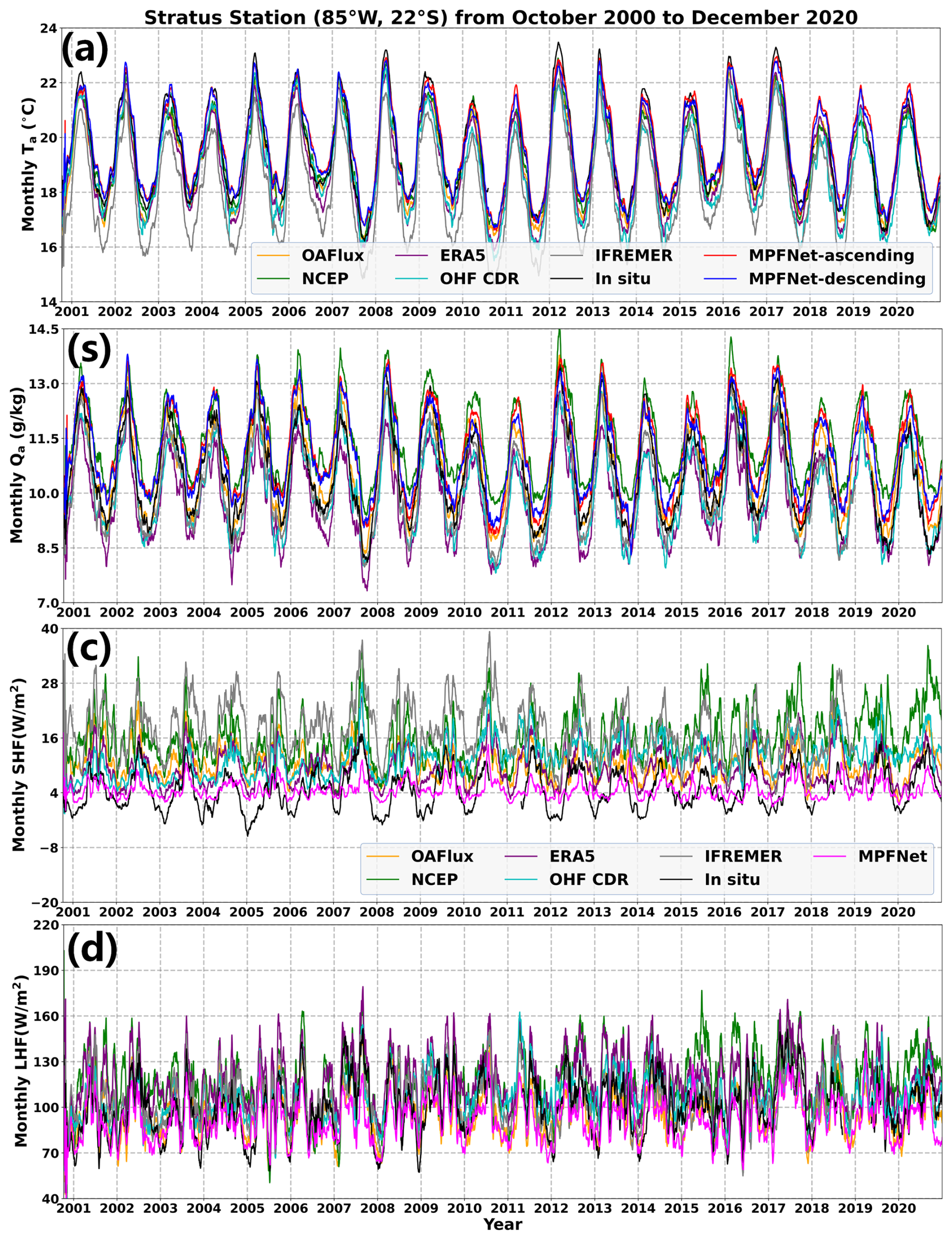
Figure 6 Monthly time series comparison at the Stratus station (85° W, 22° S) from October 2000 to December 2020. Panels (a)–(d) show T_a, Q_a, SHF, and LHF, respectively. OAFlux, NCEP, ERA5, OHF CDR, IFREMER, and MPFNet retrievals are compared with in situ observations. For T_a and Q_a, the MPFNet ascending and descending retrievals are shown separately, whereas for SHF and LHF the MPFNet estimates are shown as a single series.

At the NTAS Station in the Atlantic, where conditions are warm and humid with monthly mean T_a above 24 °C and Q_a above 14 g kg⁻¹, the SSM/I dataset consistently yields the lowest RMSEs, outperforming the other five datasets with significantly improved accuracy and clear advantages (Fig. 7).

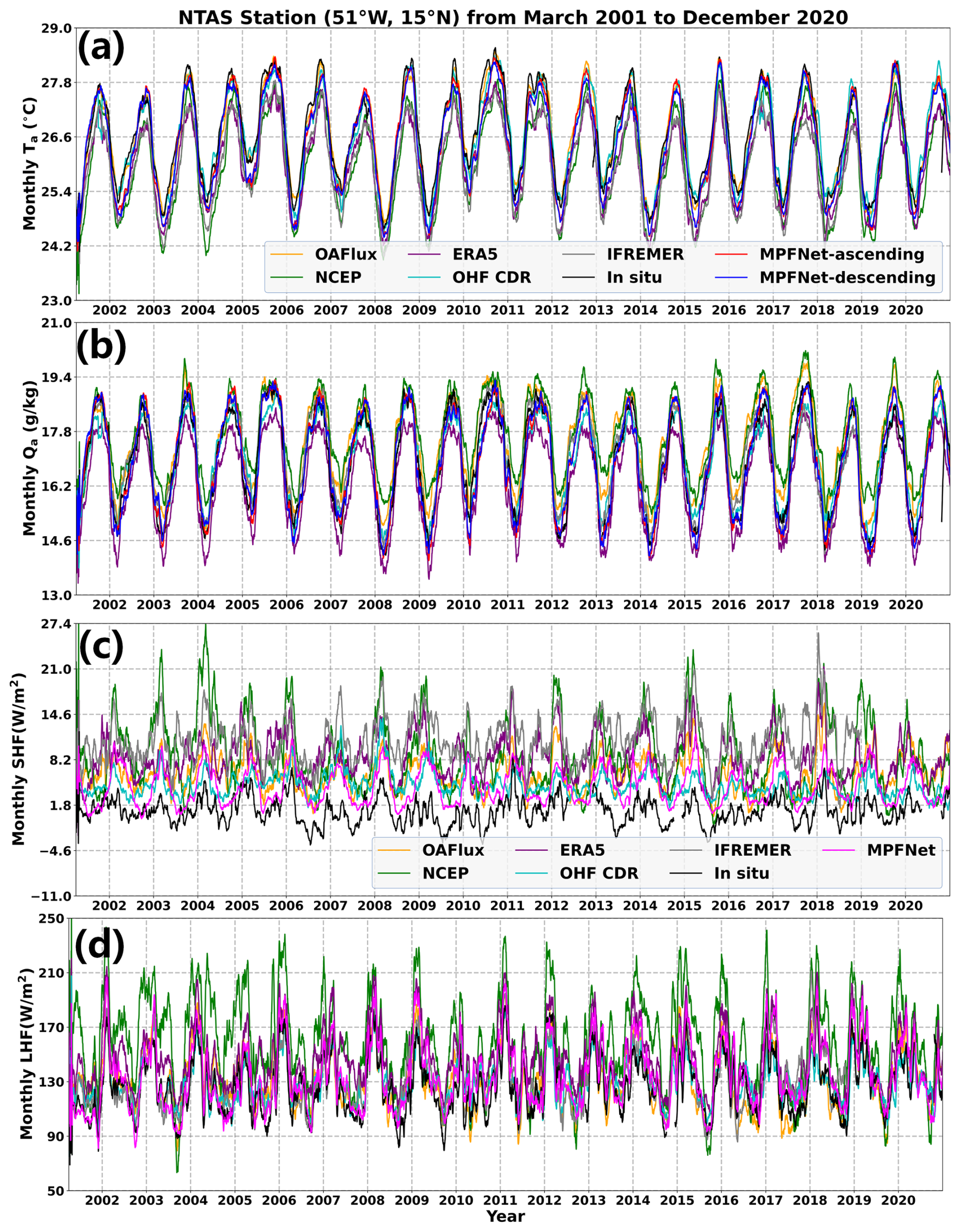
Figure 7 Monthly time series comparison at the NTAS station (51° W, 15° N) from March 2001 to December 2020. Panels (a)–(d) show T_a, Q_a, SHF, and LHF, respectively. OAFlux, NCEP, ERA5, OHF CDR, IFREMER, and MPFNet retrievals are compared with in situ observations. For T_a and Q_a, the MPFNet ascending and descending retrievals are shown separately, whereas for SHF and LHF the MPFNet estimates are shown as a single series.

4.3 Global Performance of Different Heat Flux Datasets

In this section, we evaluate the global performance of various heat flux products, comparing their differences and similarities in spatial distribution, temporal variability, and long-term trends. These comparisons provide a systematic overview of the consistency and discrepancies among different datasets and offer a basis for assessing the performance of the DeepFlux dataset relative to buoy observations. Figures 8–9 present global spatial distribution of the annual mean T_a, Q_a, SHF and LHF for different products in 2018.

The global T_a distributions from all datasets exhibit high consistency, sharing similar spatial patterns with maxima concentrated along the equator, averaging between 25 and 30 °C, and decreasing toward the poles. High Q_a values are mainly found over tropical oceans, particularly in the western Pacific warm pool and Indian Ocean, with averages ranging from 15 to 25 g kg⁻¹. In contrast, Q_a is lowest at high latitudes, approaching 0–5 g kg⁻¹ (Fig. 8).

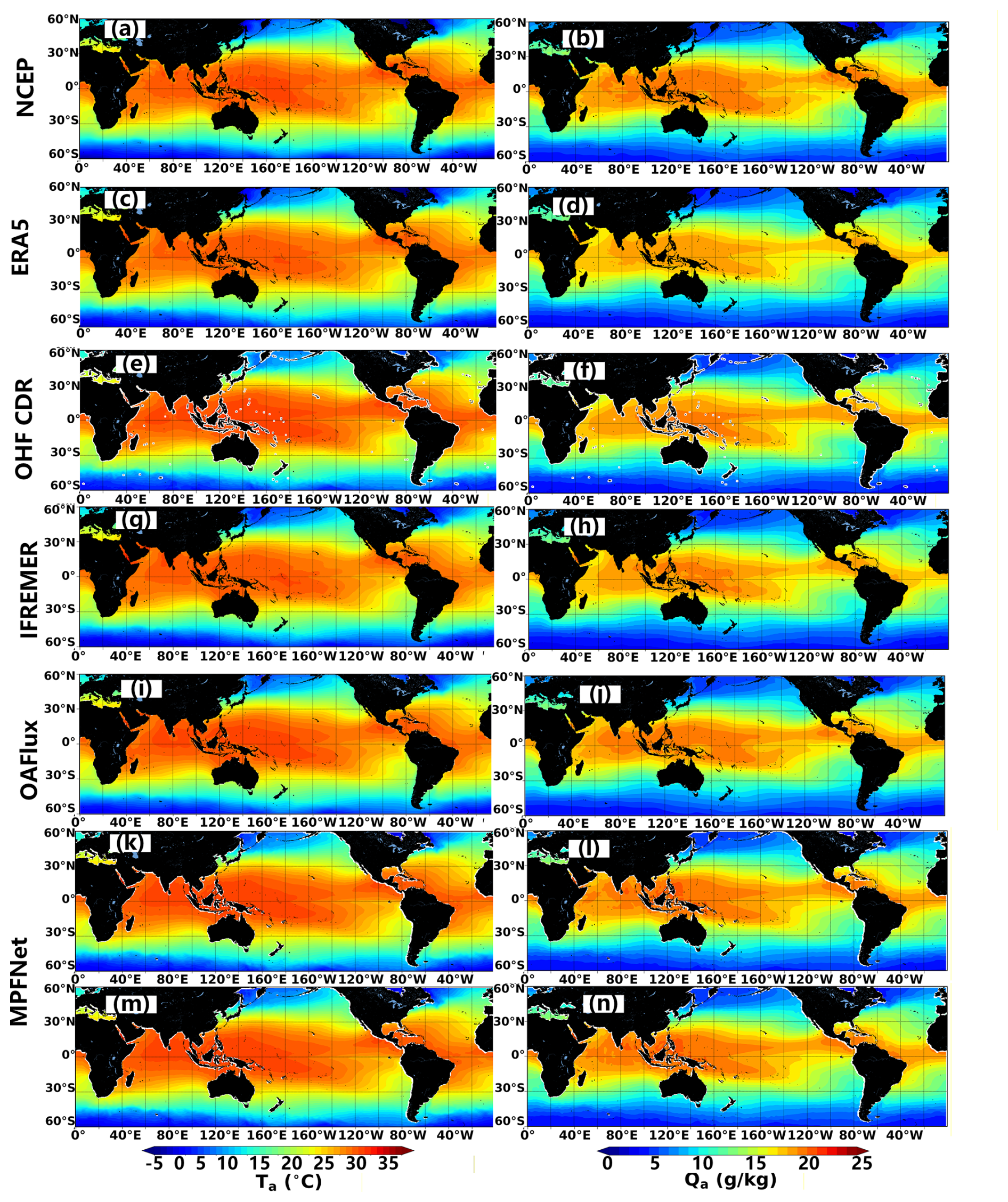
Figure 8 Global spatial distribution of the annual mean T_a and Q_a in 2018 from different products. The left column shows T_a and the right column shows Q_a. Panels (a) and (b) correspond to NCEP, (c) and (d) to ERA5, (e) and (f) to OHF CDR, (g) and (h) to IFREMER, and (i) and (j) to OAFlux. Panels (k) and (l) and (m) and (n) show the MPFNet retrievals from the ascending and descending orbits, respectively.

Positive SHF indicates heat transfer from ocean to atmosphere, while negative values reflect the opposite. SHF displays a clear zonal structure, with higher values over the North Atlantic and North Pacific, and lower values in equatorial and tropical regions. The IFREMER dataset shows an overestimation tendency in the mid-to-high latitudes of the Southern Hemisphere. Positive LHF denotes latent heat release from ocean to atmosphere, with maxima observed in the central Pacific, northwestern Pacific, and western Atlantic, where offshore winds transport cold, dry continental air over warm currents like the Kuroshio and Gulf Stream (Chou et al., 1997), driving strong air-sea heat exchange. The NCEP dataset tends to overestimate LHF, while the LHF retrieved by MPFNet aligns more (Fig. 9).

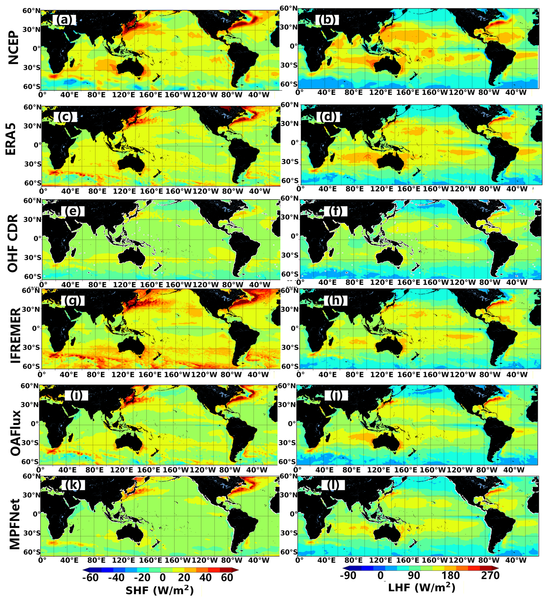
Figure 9 Global spatial distribution of the annual mean SHF and LHF in 2018 from different products. The left column shows SHF and the right column shows LHF. Panels (a) and (b) correspond to NCEP, (c) and (d) to ERA5, (e) and (f) to OHF CDR, (g) and (h) to IFREMER, (i) and (j) to OAFlux, and (k) and (l) to MPFNet.

Figure 10 presents the temporal evolution of monthly mean values from different heat flux datasets. For T_a, OAFlux, NCEP, ERA5, and IFREMER all show an underestimation trend, with IFREMER exhibiting the lowest monthly T_a, generally below 17.5 °C. For Q_a, NCEP shows a clear overestimation, while ERA5 consistently underestimates, with monthly means remaining below 11.4 g kg⁻¹. SHF and LHF are strongly correlated with T_a and Q_a; thus, OAFlux, NCEP, ERA5, and IFREMER tend to overestimate both SHF and LHF. In contrast, the DeepFlux dataset shows lower monthly means, with SHF ranging from 4–9 W m⁻² and LHF from 80–90 W m⁻². Notably, between 2000 and 2006, the OHF-CDR dataset displays significant discrepancies, consistently reporting the lowest monthly SHF and LHF.

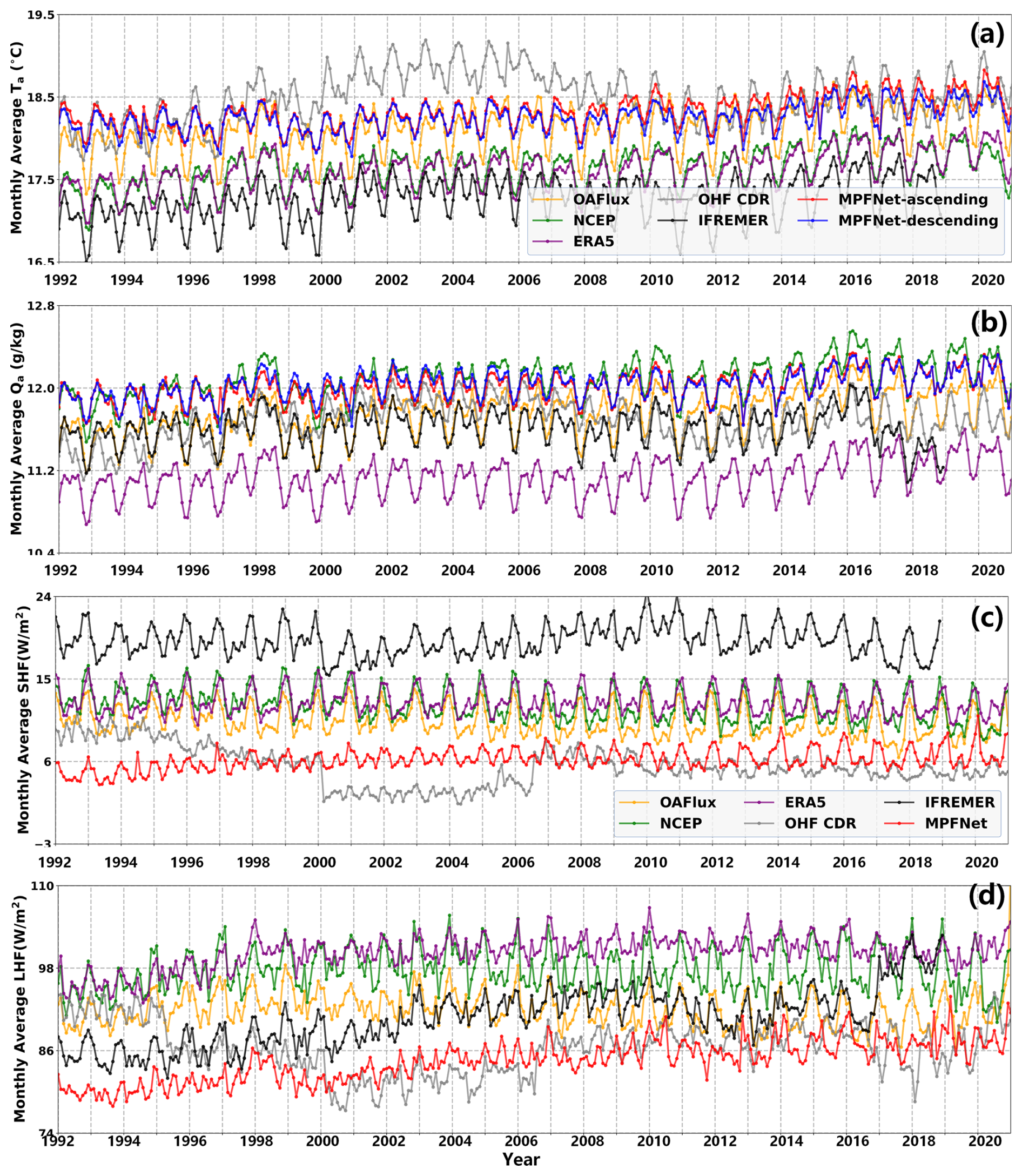
Figure 10 The temporal evolution of the monthly average of global (a) T_a, (b) Q_a, (c) SHF and (d) LHF for different products from 1992 to 2020.

5 DeepFlux Reveals Trends and Drivers of SHF and LHF

To investigate the global trends in SHF and LHF and their underlying causes, trend analyses were conducted on SHF, LHF, and their related variables (i.e., sea-air temperature difference and sea-air humidity difference). Trend calculations were based on the annual average values for all years from 1992 to 2020. Figure 11 shows the linear trends of global SHF, LHF, sea-air temperature difference, and sea-air humidity difference, where positive and negative values indicate increasing and decreasing trends, respectively. The overall trend of SHF in global oceans is relatively weak (Fig. 11a), with most regions showing trends close to zero. Significant positive trends are primarily concentrated in western boundary current regions such as the Kuroshio Current, Gulf Stream, and Brazil Current, where the ocean's release of sensible heat to the atmosphere has slightly increased, with an average maximum of 8 W m⁻². Compared to SHF, LHF exhibits a more pronounced global positive trend (Fig. 11b), with significant positive trends observed in western boundary current regions such as the central-eastern North Pacific, Kuroshio Current, Gulf Stream, East Australian Current, Brazil Current, and Agulhas Current. In these ocean regions, evaporation has significantly increased, leading to a notable rise in latent heat released to the atmosphere. LHF has increased significantly, with the maximum positive trend reaching 16 W m⁻², showing a stronger trend than SHF. The global sea-air temperature difference between the ascending and descending tracks exhibits high consistency (Fig. 11c, d), showing very similar spatial structures and magnitudes. The sea-air temperature difference in most global ocean areas exhibits a positive trend, indicating that the relative surface air temperature of the ocean is rising faster than the atmospheric temperature on a global scale. The trend in the global sea-air temperature difference shares a similar spatial structure with SHF, with their spatial distributions largely aligning. The sea-air humidity difference is a key variable linking the trends of LHF and SST. The global sea-air humidity difference in both ascending and descending orbits exhibits high consistency (Fig. 11e, f), with most regions showing a positive trend. This indicates that the humidity at the global ocean surface is increasing faster than atmospheric humidity. The global sea-air humidity difference trend is highly consistent with the LHF trend. On the other hand, the global sea-air temperature difference and sea-air humidity difference trends exhibit similar spatial structures.

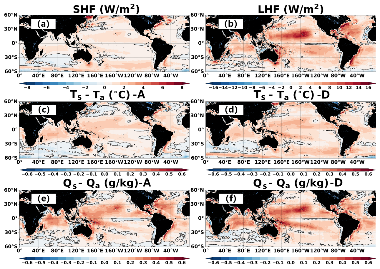
Figure 11 Linear trends (per decade) of global (a) SHF, W m⁻², (b) LHF, W m⁻², T_s−T_a (°C) for (c) ascending and (d) descending orbits, Q_s−Q_a (g kg⁻¹) for (e) ascending and (f) descending orbits, calculated from annual mean fields for 1992–2020. Positive values indicate increasing trends.

To further investigate the primary drivers of global ocean heat flux trends, it is necessary to separately examine the decadal trends in SST, Q_s, and model-reconstructed T_a and Q_a. Figure 12 shows the decadal linear trends in global SST, Q_s, T_a, and Q_a, where positive and negative values indicate increasing and decreasing trends, respectively. Most global ocean regions exhibit a clear positive trend in SST (Fig. 12a), with significant warming concentrated in the North Pacific, Indian Ocean, and western boundary current regions, reaching a maximum increase of 0.8 °C. In some areas, such as off the coast of Peru and parts of the South Pacific, SST trends are near zero or even negative, indicating localized cooling. Global Q_s exhibits a similar upward trend (Fig. 12b), with significant positive trends in the North Pacific, Indian Ocean, and western boundary current regions. The Clausius-Clapeyron relationship indicates that higher temperatures result in greater Q_s. The spatial distribution of Q_s trends in these regions aligns closely with temperature trends, consistent with the Clausius-Clapeyron relationship. The spatial distribution structure of the global average atmospheric temperature trend is similar to that of SST (Fig. 12c, d), showing an overall upward trend, though the increase is smaller than that of SST. The increase is notably reduced in the subtropical and equatorial eastern Pacific regions. The global average atmospheric humidity shows an overall positive trend (Fig. 12e, f), though the increase is far smaller than that of Q_a. In the equatorial central and eastern Pacific regions, the positive trend of Q_a weakens, and even shows a slight negative trend in some local areas, with significant spatial variability. We caution that inferred long-term trends in T_s (and derived Q_s) may depend on the chosen SST analysis, because operational changes and time-dependent bias referencing in some SST analyses can introduce inhomogeneities that affect trend estimates (e.g., Yang et al., 2021; ESA SST CCI Climate Assessment Report). Therefore, the SST-related trend interpretation should be viewed as supportive evidence, while the primary contribution of DeepFlux lies in the observation-constrained orbit-sampled T_a, Q_a, SHF and LHF fields validated against in situ measurements.

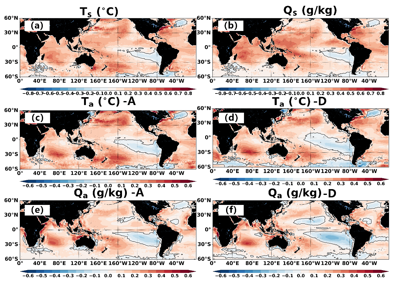
Figure 12 Linear trends (per decade) of global (a) T_s (°C), (b) Q_s (g kg⁻¹), T_a (°C) for (c) ascending and (d) descending orbits, Q_a (g kg⁻¹) for (e) ascending and (f) descending orbits, calculated from annual mean fields for 1992–2020. Positive values indicate increasing trends.

Compared with traditional reanalysis and blended products such as ERA5, IFREMER, and OAFlux, DeepFlux provides the first long-term, daily, satellite-derived global heat flux record (1992–2020) with seamless coverage, which significantly improves the representation of fine-scale features and long-term changes in key dynamic regions. In western boundary current regions (e.g., Kuroshio, Gulf Stream, Brazil Current), DeepFlux resolves stronger local gradients and more coherent positive trends of SHF and LHF, revealing intensified ocean-atmosphere exchanges that are often underestimated in coarse-resolution reanalyses. In tropical regions, DeepFlux highlights spatially heterogeneous changes in sea-air humidity difference and latent heat flux, offering new insight into the coupling between SST warming patterns and atmospheric moisture transport. The improved temporal continuity and observational grounding of DeepFlux add substantial value to long-term trend analyses, helping to reduce uncertainties introduced by model-based products and enhancing our understanding of regional climate variability and air-sea interaction processes over nearly three decades. Overall, the global average SST increase has led to a significant increase in Q_s, consistent with the Clausius-Clapeyron relationship. This is consistent with previous research findings, which indicate that changes in SST are closely related to changes in the sea-air humidity difference. The increase in T_a is found to be smaller than that of SST, leading to a larger sea-air temperature difference. Similarly, the increase in Q_a is smaller than that of Q_s, resulting in an expanded sea-air humidity difference. This expansion in the humidity difference, particularly in western boundary current regions such as the Kuroshio Current, the Gulf Stream, and the Brazil Current, becoming the primary factor driving the intensification of the LHF (Chen and Wang, 2024; Leyba et al., 2019). Similarly, the trend of SSTincrease is greater than that of T_a increase, leading to an increase in the sea-air temperature difference. The SHF is directly proportional to the sea-air temperature difference; the larger the sea-air temperature difference, the larger the SHF, thereby driving the strengthening of the SHF across global oceans. On the other hand, the rise in SST in western boundary current regions such as the Kuroshio Current, the Gulf Stream, and the Brazil Current may trigger stronger turbulent mixing, allowing more heat to be transferred from the ocean to the atmosphere, thereby enhancing the SHF (Leyba et al., 2019; Tang et al., 2024; Yu and Weller, 2007).

6 Code and data availability

The global open-ocean heat flux dataset and deep-learning models developed in this study are publicly released, as summarized below:

1. Daily global heat flux datasets. We provide a complete global daily gridded dataset of surface air temperature (T_a), specific humidity (Q_a), sensible heat flux (SHF), and latent heat flux (LHF) for the period 1992–2020. The dataset was generated by integrating SSM/I-derived variables (surface wind speed, cloud liquid water, water vapor, and rain rate) with OISST data, followed by reconstruction using the GDCM model and inversion with the MPFNet framework. The products have full global coverage at 1° × 1° spatial resolution. Validation against in situ observations shows RMSEs of 0.53 °C for T_a, 0.70 g kg⁻¹ for Q_a, 5.53 W m⁻² for SHF, and 25.28 W m⁻² for LHF.

2. Deep learning model. The Flux Model consists of the GDCM and MPFNet models. The trained versions of the GDCM and MPFNet models are shared. These can be directly applied to other satellite inputs or adapted for further fine-tuning. The GDCM model leverages spatiotemporal convolution and attention to complete missing data, while MPFNet fuses Fourier Neural Operators and ResNet modules to retrieve T_a and Q_a from multi-source inputs.

All datasets and codes are openly accessible without restrictions. They can be accessed at repository under https://doi.org/10.12157/IOCAS.20250823.001 (Wang et al., 2025b), with data available in NetCDF format. The repository also includes model scripts written in Python for data reconstruction and inversion, along with detailed documentation to facilitate reproduction and extension of this work. If you want to download without registering you can visit https://zenodo.org/records/17160579 (last access: 23 April 2026).

SSMI was downloaded from Remote Sensing Systems (https://www.remss.com/missions/ssmi/, last access: 23 April 2026) and was available from https://www.remss.com/missions/ssmi/ (last access: 23 April 2026). The NDBC buoy data was acquired from http://www.ncdc.noaa.gov (last access: 23 April 2026). Buoy measurements from GTMBA were downloaded from http://pmel.noaa.gov (last access: 23 April 2026). The ICOADS was from https://www.ncei.noaa.gov/products/international-comprehensive-ocean-atmosphere-data-set (last access: 23 April 2026). The WHOI buoy was from https://uop.whoi.edu/currentprojects/ReferenceDataSets.html (last access: 23 April 2026). The OHF CDR was available from https://www.ncei.noaa.gov/access/metadata/landing-page/bin/iso?id=gov.noaa.ncdc:C01561 (last access: 23 April 2026). The IFREMER v4.1 was from ftp://ftp.ifremer.fr/ifremer/cersat/products/gridded/flux-heat/ (last access: 23 April 2026) (/ifremer/dataref/heat-fluxes). The NCEP was from https://psl.noaa.gov/data/gridded/data.ncep.reanalysis.surface_gauss.html last access: 23 April 2026). The ECMWF ERA5 was available from https://doi.org/10.24381/cds.adbb2d47 (Hersbach et al., 2023). The OAFlux was available from https://oaflux.whoi.edu/data-products/ (last access: 23 April 2026).

7 Conclusion

In this study, we developed DeepFlux the first global, seamless, daily ocean surface heat flux dataset derived solely from SSM/I to SSMIS passive microwave observations, together with OISST SST and limited ERA5 infill for missing dates, spanning 1992–2020 with 1° × 1° resolution. Using a two-step deep learning approach, we first employed the GDCM to reconstruct missing satellite observations and then applied the MPFNet to retrieve T_a, Q_a, SHF, and LHF from SSM/I-derived SSW, CLW, WV, and RR. The separation of T_a and Q_a into ascending and descending track channels provides additional diurnal variability information often absent in traditional datasets.

The heat flux dataset developed in this study demonstrates significantly improved spatial completeness and accuracy compared to mainstream products such as NCEP, ERA5, OHF-CDR, IFREMER, and OAFlux, the test set, consisting of 21 613 records from 2018, shows excellent performance with RMSEs of 0.53 °C for T_a, 0.70 g kg⁻¹ for Q_a, and 5.53 and 25.28 W m⁻² for SHF and LHF, respectively. It exhibits higher stability and reduced systematic bias, especially in tropical and mid-latitude regions. Independent validation using monthly data from the NTAS, Stratus, and WHOTS buoys further confirms its robustness across diverse oceanic environments. With a continuous 28-year temporal coverage, the dataset extends the duration and completeness of global ocean heat flux records. Its high accuracy supports improved parameterization in climate models and provides a reliable data source for studying air-sea interactions and their role in driving atmospheric and oceanic circulation.

Importantly, DeepFlux fills key observational gaps in the tropics, western boundary currents, and other dynamically active regions (e.g., Kuroshio, Gulf Stream, Brazil Current), where existing products often exhibit large retrieval errors or coarse spatial/temporal coverage. The dataset's seamless daily continuity over nearly three decades offers a unique resource for long-term climate analyses, enabling a clearer assessment of multi-decadal trends in air–sea fluxes and their physical drivers. Our results show that DeepFlux captures the spatial structure and intensification of SHF and LHF trends with higher fidelity than existing datasets, particularly highlighting the role of sea–air humidity and temperature differences in driving flux variability in high-energy regions.Reliance on SSM/I passive microwave data may introduce errors under severe weather conditions, such as interference from thick cloud cover. The retrieval accuracy of SHF and LHF is influenced by the quality of SSW input, and some SSM/I wind products contain considerable errors, necessitating additional correction steps. These limitations highlight future improvement directions: integrating data from additional satellite sensors such as AMSR, SSM/I, and WindSat to enhance spatial coverage and reduce uncertainties from single-sensor reliance; and incorporating high-resolution reanalysis or in situ observations to further refine the retrieval of T_a and Q_a, thereby improving the accuracy of SHF and LHF estimates.