Monitoring dry snow metamorphism using 4D tomography across 20 experimental conditions

Refined observations of the temporal evolution of snow microstructure are crucial for improving the understanding and modeling of snow metamorphism. X-ray tomography has opened new possibilities for observing the microstructure of dry snow by enabling 3D imaging of the ice and air arrangement with micrometric resolution. The development of cells that control the thermal boundary conditions of a snow sample during scanning has made in-situ monitoring of microstructural changes during metamorphism possible. However, such data sets remain scarce and are often limited in terms of the snow evolution conditions explored. In this work, we use highly resolved X-ray tomography to characterize the temporal evolution of dry snow microstructure under a wide range of thermal boundary conditions. We designed a snow-metamorphism cell to continuously control the temperature at the boundaries of a centimeter-sized snow sample directly inside the tomograph. Using this setup, we conducted a total of 20 snow metamorphism experiments, covering mean snow temperatures from −3 to −17 °C, snow temperature gradients from 0 to 100 K m⁻¹, and five initial snow samples with varying snow types, densities, and specific surface areas. Each experiment lasted 7 d, during which tomographic measurements were performed every 4 h at a spatial resolution of 8.5 µm. We provide a unique set of 4D data in .zarr format, consisting of time series of binary 3D images of snow undergoing the aforementioned experiments. These images are particularly well-suited for investigating local processes, such as the interface growth velocity, as well as the geometrical properties of snow, such as specific surface area, chord length distribution, or surface curvature, to name just a few. Computing these properties could help to model their evolution during dry snow metamorphism. In addition, videos showing the temporal evolution of the snow microstructure for the 20 experiments are provided. The data set and the videos are available at https://doi.org/10.1594/PANGAEA.992556 (Dick et al., 2026).

1 Introduction

Snow microstructure refers to the three-dimensional arrangement of ice, air, and, sometimes, liquid water at the sub-millimeter scale. It controls the physical and mechanical properties of snow and thus the behavior of the snowpack at larger scales, such as the avalanche release (e.g. Schweizer et al., 2003), the hydrology of the mountain regions (e.g. Holko et al., 2011), or the interaction between climate and earth surface (e.g. Dumont et al., 2014). This microstructure is in constant evolution, notably through shape transformations driven by thermodynamic processes, known as snow metamorphism (e.g. Yosida et al., 1955; Colbeck, 1983). Dry snow metamorphism refers more specifically to the transformations that occur in dry snow, in the absence of liquid water.

Dry snow metamorphism is traditionally classified into two categories. If the snow is in near-isothermal conditions, the microstructure undergoes equi-temperature metamorphism (ETM); otherwise, it undergoes temperature gradient metamorphism (TGM). ETM is caused by thermodynamic instabilities driven by curvature gradients at the ice-air interfaces (Thomson, 1871). In contrast, TGM is caused by thermodynamic instabilities driven by temperature gradients in the snow (Colbeck, 1983). They result in different microstructure transformations. Mainly, ETM leads to the rounding and sintering of the snow grains (Colbeck, 1980), while TGM leads to the faceting and coarsening of the snow grains, without grain sintering (Colbeck, 1983). The resulting snow types are rounded grains for ETM and faceted crystals and depth hoar for TGM, as defined in the international classification for seasonal snow on the ground (Fierz et al., 2009). However, despite these standard features, variations exist in snow transformation within the same metamorphism class. Indeed, the intensity of the temperature gradients (e.g. Akitaya, 1974; Furukawa and Kohata, 1993; Pfeffer and Mrugala, 2002; Wang and Baker, 2014), the absolute temperature at which the transformation occurs (e.g. Kamata et al., 1999; Kaempfer and Schneebeli, 2007; Bouvet et al., 2023), and the initial properties of the transforming snow (e.g. Akitaya, 1974; Marbouty, 1980; Sturm and Benson, 1997; Pfeffer and Mrugala, 2002), are all factors that affect the evolution of the microstructure. For example, a different type of depth hoar, called hard depth hoar, can be obtained during TGM for specific initial snow type and density (Pfeffer and Mrugala, 2002). Kaempfer and Plapp (2009) showed that ETM conducted at temperatures between −2 and −54 °C results in drastically different stages of rounded grains, as low temperatures slow down the snow transformation.

To access dry snow microstructure and its evolution during metamorphism, a breakthrough development has been the introduction of X-ray tomography (Brzoska et al., 1999; Coléou et al., 2001; Lundy et al., 2002). Because air and ice have different X-ray attenuation properties, the 3D microstructure of snow at the micrometer scale can be retrieved from absorption tomographic measurements of snow samples. Over the last 25 years, various methods have been developed to monitor the temporal evolution of snow microstructure during dry snow metamorphism using X-ray tomography. A first approach involves scanning different snow samples extracted at regular time intervals from a snow layer undergoing snow metamorphism, either in nature or in a cold laboratory (e.g. Flin et al., 2004; Srivastava et al., 2010; Calonne et al., 2014; Bouvet et al., 2023). Snow evolution is thus captured by imaging different snow samples of the same snow layer. In some cases, snow samples can be impregnated for conservation until tomography (e.g. Brzoska et al., 1999; Coléou et al., 2001; Heggli et al., 2009). A second approach, referred here as in-situ monitoring, involves scanning the same snow sample at regular time intervals, with the snow sample undergoing snow metamorphism directly inside the tomograph (e.g. Schneebeli and Sokratov, 2004; Pinzer and Schneebeli, 2009; Kaempfer and Plapp, 2009; Chen and Baker, 2010; Pinzer et al., 2012; Calonne et al., 2015; Hammonds et al., 2015; Wiese and Schneebeli, 2017a; Granger et al., 2021; Li and Baker, 2022). Since the same snow sample is scanned, the evolution of the ice-air interface of the snow grains can be tracked, provided that the scanning frequency is appropriate. For this approach, a dedicated environmental cell mounted in the tomograph is used to hold the snow sample and control its boundary temperatures. Two types of cells exist: cells that operate at ambient temperature, which can operate in a broad range of tomographs but need to include an efficient system of thermal insulation (Enzmann et al., 2011; Rolland du Roscoat et al., 2011; Calonne et al., 2015), and cells that operate at negative temperatures in the cold laboratory where the lab-tomograph is also placed (Schneebeli and Sokratov, 2004; Pinzer and Schneebeli, 2009; Wiese and Schneebeli, 2017a).

In-situ monitoring of snow samples undergoing metamorphism using X-ray tomography and an environmental cell has been done in the past (e.g. Flin et al., 2004; Schneebeli and Sokratov, 2004; Kaempfer and Plapp, 2009; Pinzer and Schneebeli, 2009; Srivastava et al., 2010; Pinzer et al., 2012; Riche et al., 2013; Wang and Baker, 2014; Calonne et al., 2014; Hammonds et al., 2015). They differ in terms of spatial and temporal resolution of tomography, duration of the metamorphism, boundary conditions (temperature and mechanical load), and initial snow samples. Most studies focus on monitoring a single snow metamorphism, with a unique set of boundary conditions and initial snow, partly because such experimental work is time-consuming. Some of the more extensive studies on snow metamorphism monitoring are described hereinafter. Pinzer et al. (2012) studied three cases of TGM, in which similar initial snow samples, made of rounded grains, were subjected to a temperature gradient of 50 K m⁻¹ at three different mean temperatures of −3.4, −8.1, and −7.6 °C for 11, 16, and 28 d, respectively. Samples were scanned every 8 or 4 h at a spatial resolution of 25 or 18 µm, depending on the time-series. Grain interface tracking was performed for the first time, so that the amount of ice growth or decay at any location of the ice-air interfaces during metamorphism could be assessed. Kaempfer and Schneebeli (2007) measured four time series of snow evolving under ETM for a large range of mean temperature (from −1.6 to −54 °C), starting from fresh snow samples, during nearly one year. Tomography was done monthly at a resolution of 10 µm. Especially, they highlighted the strong dependency of ETM on temperature. Wang and Baker (2014) carried out 18 experiments of intense TGM, with variations in the initial snow types (precipitation particles, small and large rounded particles), temperature gradients (from 100 to 500 K m⁻¹), but for a unique mean temperature of −4 °C. Tomography was performed every 4 h at a spatial resolution of 15 µm. The focus was on studying the SSA evolution during the early stage of TGM, so the experiments were short, lasting up to 48 h only. Finally, Wiese and Schneebeli (2017b) carried out 13 experiments of both ETM and TGM, with variations in temperature gradient (from 0 to 95 K m⁻¹) and mean temperature (from 4.1 13.7 °C), but using initial snow samples made of sieved rounded grains of similar density and specific surface area. These metamorphism experiments were combined with snow settling, which was imposed on the snow samples by placing a load on top, the focus being to study the interaction between temperature gradient and settling on the snow microstructure evolution.

Yet, there is a need for a broader range of time series of snow microstructure images at high spatial and temporal resolutions. Such data would be required to better understand and model dry snow metamorphism, including the role of the temperature conditions and initial snow (Pfeffer and Mrugala, 2002). The recent studies of Krol and Löwe (2018) and Braun et al. (2025) point out the lack of experimental time series of snow images to develop and evaluate the models of dry snow metamorphism, and especially the modeling of the specific surface area. Indeed, Krol and Löwe (2018) underlines the need for high-resolution data to obtain better evaluation of the interface growth velocity, which appears to control the specific surface area evolution, according to Eq. 14 in Krol and Löwe (2018). Braun et al. (2025) also highlights the need for experiments with systematic variations of the boundary conditions and initial conditions to parametrize the proposed evolution law of the specific surface area of snow (Eq. 5 in Braun et al., 2025). Such evolution laws of microstructure properties are needed to improve the representation of the snow microstructure, and hence, the physical properties of snow, in detailed snowpack models such as CROCUS or SNOWPACK (Vionnet et al., 2012; Lehning et al., 2002). Currently, the evolution laws of density and specific surface area in the detailed snowpack models are not fully satisfactory. For example, it was shown that the SNOWPACK model overall underestimates SSA compared to field measurements, and the Crocus model tends to underestimate densification for fresh snow and, inversely, to overestimate densification for depth hoar (Schleef et al., 2014; Calonne et al., 2020).

The present work contributes to filling this data gap. We present a unique set of time series of 3D images of 20 scenarios of dry snow metamorphism, monitored with time-lapse tomography at a spatial resolution of 8.5 µm and a temporal resolution of 4 h. For that, we developed a snow metamorphism cell, referred to as CellCold, that enables in situ monitoring. Using this cell, we varied the average temperature (−3, −8, and −17 °C), the temperature gradient (0, 10, 40, and 100 K m⁻¹), and the initial snow (varying snow types, density, and specific surface area). Each experiment lasted 7 d. The provided data set consists of 20 time series of 3D segmented images of snow microstructure, ready for further computations of snow properties as well as further analysis of the local processes, such as the evaluation of grain growth by interface tracking. Videos of the evolving snow microstructures are also provided.

The paper is organized as follows. Section 2 presents the snow metamorphism cell. Section 3 describes the experiments, including the experimental work in the cold laboratory and the image processing to obtain the 3D binary images. Finally, Sect. 4 presents the resulting data set, consisting of 20 time series of 3D images of snow undergoing metamorphism under various conditions. We also highlight in this section the potential of such data set for the understanding of dry snow metamorphism and its modeling.

2 Snow metamorphism cell

2.1 Description of CellCold

To capture the evolution of snow samples' microstructure by X-ray tomography at high spatial and temporal resolution, we designed a snow metamorphism cell, called CellCold. The development of CellCold was inspired by previously developed snow cells (Pinzer and Schneebeli, 2009; Wiese and Schneebeli, 2017a). This cell allows the continuous control of the boundary temperatures of a centimeter-sized snow sample, including during tomographic scanning. Hence, CellCold is mounted directly inside the tomograph operating in our cold room. It allows for convenient handling of snow samples, so that a sample can be easily placed and removed, and it is made from materials that do not interfere with X-rays in the field of view. Figure 1 presents a picture of CellCold mounted in the tomograph (a), as well as a schematic of the cell (b) and a picture of the sample holder (c). The cell can be divided into three parts: the temperature control part, the snow sample holder, and the electrical connections.

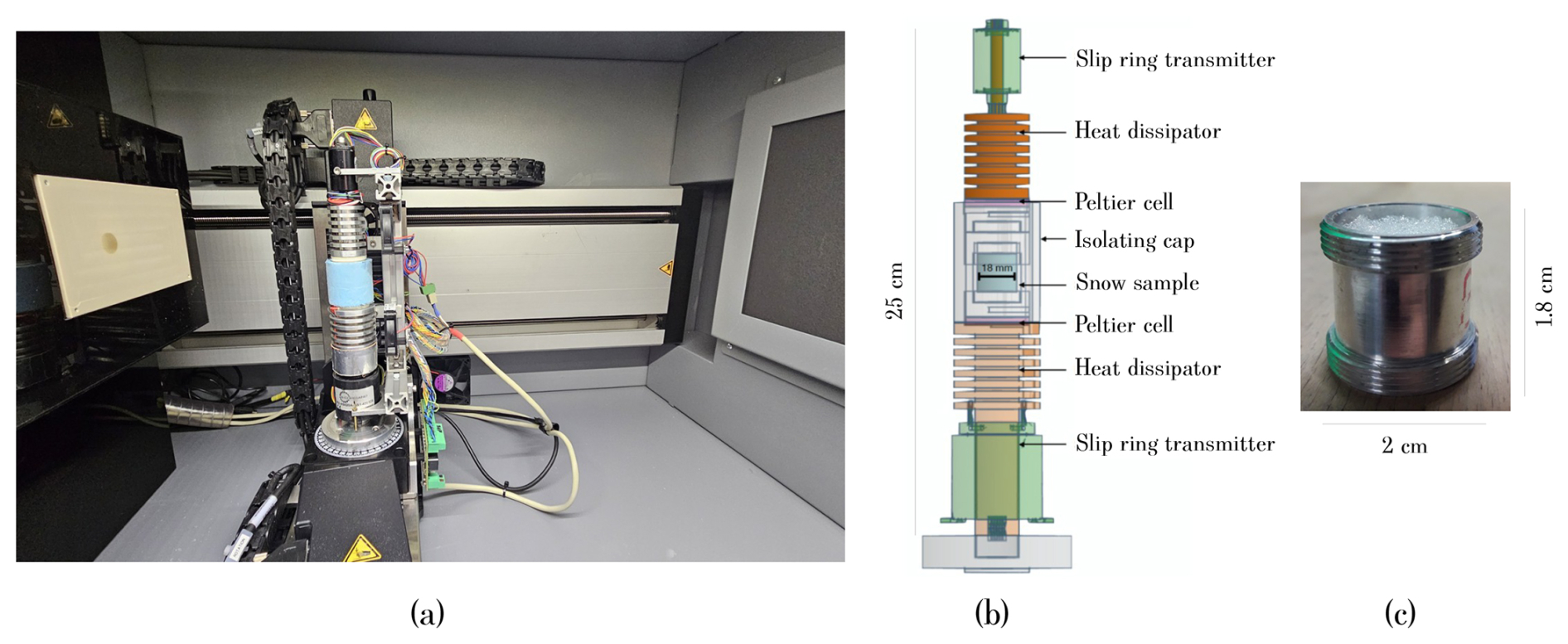
Figure 1 Illustration of the snow metamorphism cell CellCold. (a) Picture of CellCold in the tomograph chamber: X-ray source is on the left, X-ray detector is on the right, and CellCold, mounted on the rotation platform of the tomograph, is in the middle. (b) Schematic of the cell with the description of the different parts. Transparency was applied to some of the cell components, such as the polystyrene and the aluminum sample holder, for the sake of clarity. (c) Picture of an aluminum sample holder filled with snow.

To constrain the temperature at the top and the bottom of the snow sample, we use two Peltier devices located above and below the sample holder. The Peltier heat pumps are from Arctic TEC Technologies, and correspond to round single-stage thermoelectric coolers (model TEC-14,7-3,9-34,0-70-30/0-R). They are controlled using the Peltier controller TEC 1141-4A. The Peltier cells have an absolute accuracy of 0.5 K. Aluminum heat exchangers, or heat sinks, are attached to both Peltier cells to dissipate the energy produced by the Peltier. To facilitate energy transfer, the heat exchangers have fins to increase heat transfer area on the air side and are ventilated by fans.

The snow sample holder is located at the center of CellCold between each Peltier cell. It corresponds to a cylinder made of aluminum, which can hold a cylindrical snow sample of a height of 1.8 cm and a diameter of 2 cm, as shown in Fig. 1c. The central part of the holder is thin (aluminum of 0.5 mm thickness) to minimize the absorption of X-rays by the holder. The upper and lower parts of the holder are thicker (1.2 mm thick) and are threaded, so that the sample holder can be screwed onto the upper and lower Peltier cells. The sample holder is open at the top and closed at the bottom with a 5 mm thick aluminum plate. The sample holders have been produced by precision machining a single aluminum piece for each holder. Aluminum has been chosen for its relatively high thermal conductivity and moderate X-ray attenuation coefficient. The sides of the sample holder are thermally insulated from the outside using an insulating cap made of polystyrene foam 8 mm thick (blue foam visible in Fig. 1a).

At the extremities of the cell, slip rings are mounted adjacent to the heat exchangers. They allow the electrical cables, which power and control the Peltier cells, to pass through without rotating with the cell during a scan. The two models used are the slip ring B-Command RX-HS005A-QS2-00012S and the slip ring B-Command RX-HS020A-QS2-42012S. Finally, CellCold can be mounted on the rotation platform of the tomograph using screws. The final set-up in the tomograph chamber is shown in Fig. 1a.

The cell is easy to handle. In practice, when placing a new snow sample holder, the holder is first screw to the bottom part of the cell, the polystyrene foam is then slid into position, and the upper part of the cell is then screwed to the top of the holder.

2.2 Heat conduction simulation in CellCold

To estimate the quality of the temperature field inside the sample holder of CellCold and verify the effective temperature gradient experienced by the snow sample, we performed 3D heat conduction simulations. The design of the different parts of CellCold was done using the open-source parametric 3D modeler FreeCAD, and the heat conduction equations were solved using the open-source computational tool Elmer. Snow was modeled as a homogeneous medium with a density of 100 kg m⁻³ and a conductivity of 0.05 W m⁻¹ K⁻¹. To replicate the experimental conditions (see Sect. 3.1), a 2 mm thick ice layer was included at the bottom of the snow sample, with a density of 917 kg m⁻³ and a conductivity of 2.1 W m⁻¹ K⁻¹. The sample holder and Peltier devices were modeled as aluminium 6060, with a density of 2700 kg m⁻³ and a conductivity of 209 W m⁻¹ K⁻¹. The insulating foam was modeled as polystyrene with a density of 30 kg m⁻³ and a conductivity of 0.03 W m⁻¹ K⁻¹. We imposed constant temperature conditions at the external boundaries. We applied the values of the target temperatures of the Peltier cells on the top and bottom Peltier faces, and the value of the air temperature surrounding CellCold in the tomograph on the lateral sides of the insulating foam.

To illustrate our simulation results, Fig. 2 presents a simulation of heat conduction in CellCold, obtained for a gradient of 100 K m⁻¹. The top temperature was set to −3.9 °C, the bottom temperature to −2.1 °C, and the outside temperature to −3 °C, which corresponds to the mean of the top and bottom temperatures. A similar temperature setup was used during our experiments. The right panel shows the temperature field in the immediate surroundings of the sample holder, and the left panel shows the vertical temperature profile along a line drawn in the middle of the sample holder. We see that most of the temperature gradient is located in the snow, whereas almost no temperature changes occur in the ice layer. We also see that the temperature evolution with height is not strictly linear due to the vertical asymmetry of the sample holder.

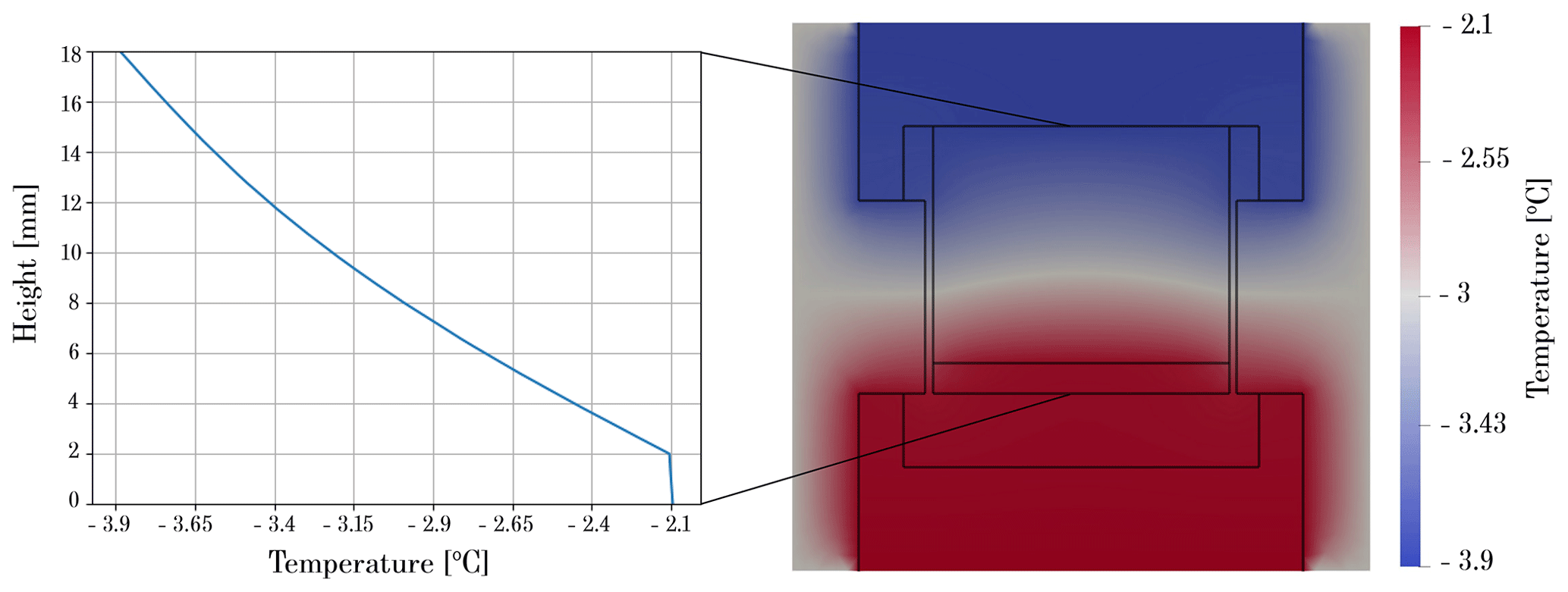
Figure 2 Simulation of the heat conduction in the cell. The right panel shows the temperature field in the immediate surroundings of the snow sample obtained for a temperature gradient of 100 K m⁻¹. The boundaries of the cell components are shown by grey solid lines. The lateral boundaries correspond to the outer surface of the polystyrene cylinder. The top and bottom boundaries correspond to the Peltier devices. We applied a top temperature of −3.9 °C, a bottom temperature of −2.1 °C, and a temperature at the lateral boundaries of the polystyrene cylinder of −3 °C. The left panel shows the corresponding vertical temperature profile in the center of the snow sample holder, filled with snow lying on the 2 mm ice layer.

We used these simulations to evaluate the effective vertical temperature gradient along the rotation axis and the effective horizontal gradient parallel to the bottom surface in the snow sample, compared to the imposed, macroscopic temperature gradient controlled by the Peltier devices. For an imposed gradient of 100 K m⁻¹, the effective vertical gradient in the snow sample is 108 K m⁻¹ with the ice layer and 97 K m⁻¹ without the ice layer. The value without the ice layer can be seen as a lower boundary of the temperature gradient for the extreme case that the ice layer decays until full disappearance during the experiment. This was observed in none of our experiments. For an imposed gradient of 40 K m⁻¹, the effective vertical gradient in snow is 44 K m⁻¹ with an ice layer and 39 K m⁻¹ without the ice layer. Finally, for an imposed gradient of 10 K m⁻¹, the effective vertical gradient in snow is 10.6 K m⁻¹ with the ice layer and 10 K m⁻¹ without the ice layer. In addition, the Peltier cells have a relative accuracy of ±0.03 °C, which results in an accuracy of ±1.7 K m⁻¹ for the temperature gradient applied to the snow samples. Hence, we roughly estimate that, during our experiment of temperature gradient metamorphism, the vertical temperature gradient experienced by the snow volume corresponds to the imposed temperature gradient with a maximum error of ±(1.7 K m⁻¹ + 10 %). Finally, for all the imposed temperature gradients, no significant effective temperature gradient was obtained along the horizontal direction in snow.

We also used the simulation to evaluate our isothermal conditions. For that, both Peltier devices impose the same temperature. In that case, the critical parameter that influences the quality of the temperature field in snow is the temperature difference between the temperature imposed by the Peltier devices and the air temperature outside CellCold, which can create a lateral temperature gradient inside the snow sample. We estimate that a difference of 2 °C was the maximum that could be punctually reached during our experiments. For a difference of 2 °C, we simulated a maximum horizontal temperature gradient of 0.16 K m⁻¹ and a maximum vertical temperature gradient of 0.016 K m⁻¹ inside the snow. Both values are insignificant and lead to equi-temperature metamorphism (ETM). This conclusion was confirmed by the analysis of the snow image obtained from the ETM experiment, for which the expected behavior for a curvature-driven snow evolution was observed.

3 Dry snow metamorphism experiments

3.1 Experimental conditions

We conducted 20 experiments to monitor dry snow metamorphism by tomography using CellCold. Five different types of initial snow samples, four temperature gradients, and three mean temperatures have been explored.

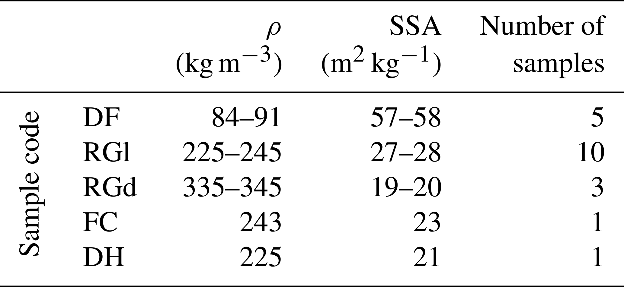
First, we describe the snow samples used as initial samples to start our experiments. These samples were either created by sieving different natural snow or directly resulted from our metamorphism experiments. Table 1 summarizes the main characteristics of the 20 initial snow samples used, including their range of density and SSA, computed from the initial 3D image of each experiment (computation described in Sect. 3.2). Visualizations of these 5 initial sample types are provided later in Sect. 4. The five different initial snow types correspond to samples of decomposing and fragmented particles, light rounded grains, dense rounded grains, faceted crystals, and depth hoar. We refer to these samples using the snow type abbreviations (Fierz et al., 2009). To differentiate the light and dense rounded grain samples, we combined the snow type with the letter “l” for light and “d” for dense.

• The samples DF refer to samples of decomposing and fragmented precipitation particles with rimed surfaces (towards graupel), with a mean density of 86 kg m⁻³ and a mean SSA of 57.5 m² kg⁻¹. They were obtained from decomposing and fragmented particles sampled at the Col de Porte field site (1325 m elevation) on the 26 January 2025. They were stored in the cold lab at −8 °C for 24 h and then sieved in the aluminum holder using a sieve with a mesh size of 4 mm. The samples were left to sinter for 5 h in the cold lab at −8 °C and then placed into the −85 °C freezer for storage until the experiment. 5 samples were made.

• The samples RGl refer to samples of rounded grains considered as light in the present study, with a mean density of 235 kg m⁻³ and a mean SSA of 27.5 m² kg⁻¹. They were obtained from the same decomposed and fragmented particles as for the DF samples, but the sieving was done with a finer sieve with a mesh size of 1.6 mm. After sieving, the RGl samples were left to sinter for 19 h in the cold lab at −8 °C, before being placed into the −85 °C freezer for storage until the experiment. 10 samples were made.

• The samples RGd refer to samples of rounded grains considered as dense, with a mean density of 340 kg m⁻³ and a mean SSA of 19.5 m² kg⁻¹. They were obtained from rounded grains stored in the cold lab of CEN at −22 °C for more than six months. Samples were made by sieving the snow in the sample holders using a sieve with a mesh size of 1.6 mm, followed by 19 h of sintering at −8 °C, before being placed into the −85 °C freezer for storage until the experiment. 3 samples were made.

• The sample FC refers to a sample of faceted crystals of density 243 kg m⁻³ and SSA of 23 m² kg⁻¹. This sample was directly obtained from one of our experiments, as it was the snow resulting from the evolution of a DF sample after 7 d of temperature gradient metamorphism at 10 K m⁻¹ at a mean temperature of −3 °C. 1 sample was made.

• The sample DH refers to a sample of depth hoar of density of 225 kg m⁻³ and SSA of 21 m² kg ⁻¹. This sample was the snow resulting from the evolution of a DF sample after 7 d of temperature gradient metamorphism at 100 K m⁻¹ at a mean temperature of −3 °C. 1 sample was made.

Table 1 Density and SSA of the different types of initial snow samples.

For each sample, a 2 mm-thick ice layer was first created on the bottom of the sample holder. The ice layer constitutes a basal vapor source and prevents the formation of an air gap when strong temperature gradients are applied, as observed in previous similar experiments (Wiese and Schneebeli, 2017b; Bouvet et al., 2023). During our experiments of temperature gradient, the ice layer tended to decrease in thickness, whereas ice deposition occurred at the top against the aluminum cap. These effects were very localized and concerned the upper and lower 3 mm parts of the sample, at most. Figure A1 of the appendix illustrates the evolution of the sample boundaries between the start and the end of an experiment with a temperature gradient of 100 K m⁻¹ at −3 °C. For the samples DF, RGl, and RGd, the snow was then sieved in the aluminium sample holder on top of the ice layer. The excess of snow at the surface was removed using a metal blade. The sample holders were then sealed with the aluminum caps to prevent snow sublimation; the cap was removed just before usage. The snow samples were stored until usage in their aluminum sample holders in a freezer at −85 °C, a temperature at which snow no longer transforms.

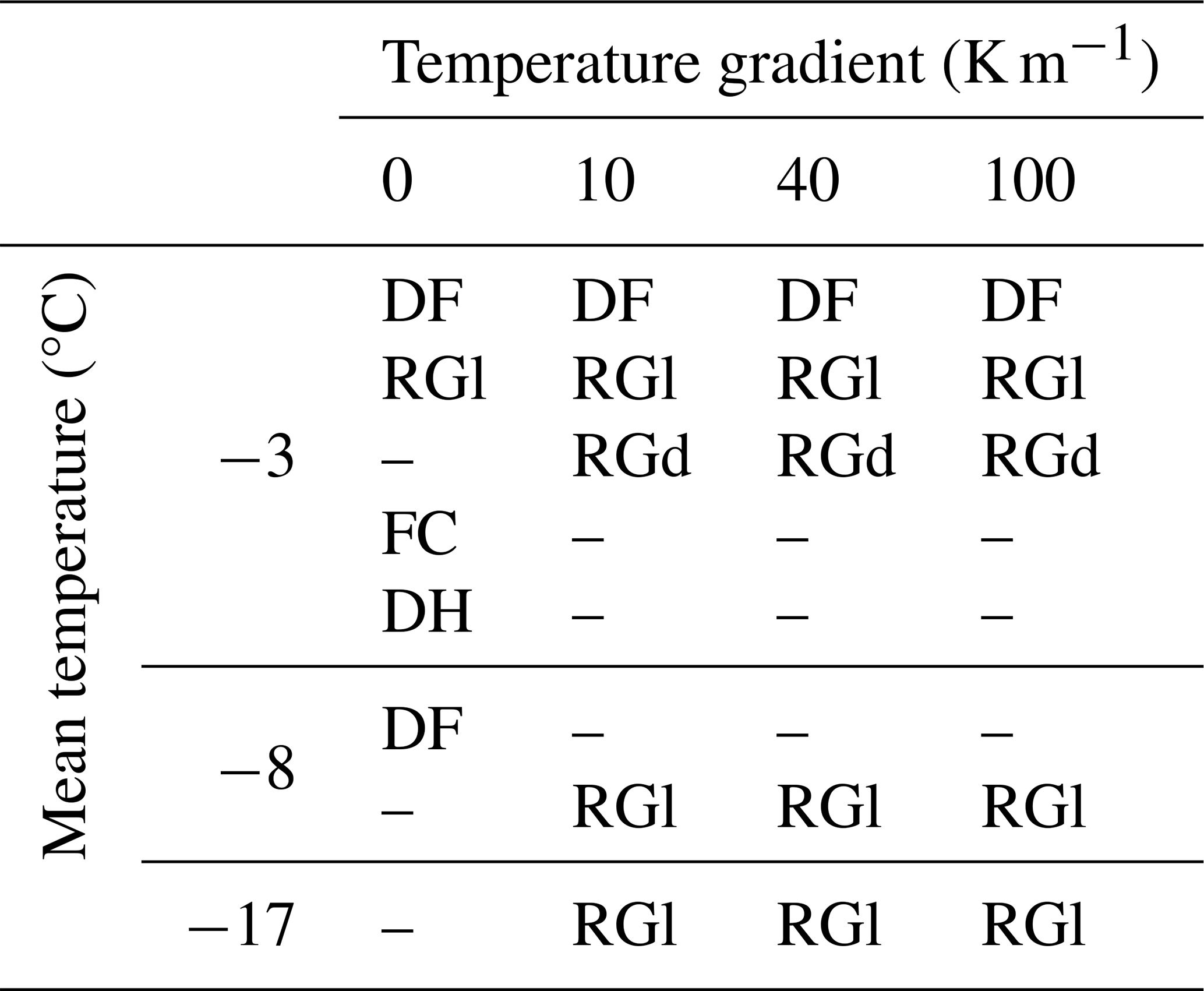
Next, we describe the temperature conditions applied to the snow samples, as synthesized in Table 2. Temperature gradients of 0, 10, 40, and 100 K m⁻¹, and ambient or mean temperatures of −3, −8, and −17 °C were explored. The ambient temperature corresponds to the temperature inside the tomograph chamber, itself controlled by the temperature of the cold lab. The top and bottom temperatures of the Peltier devices were set so that the ambient temperature corresponds to their average value, in order to reduce the lateral temperature gradients. For example, for a gradient of 100 K m⁻¹ at a mean temperature of −3 °C, the top temperature was set to −3.9 °C and the bottom temperature was set to −2.1 °C. Table 2 provides an overview of the 20 experiments carried out and the experimental conditions applied. Not all the combinations of temperature and temperature gradient were covered for all the different initial snow samples. The samples RGl were used the most systematically and cover all ambient temperatures and all temperature gradient conditions. Isothermal conditions were applied at −3 °C on the samples DF, RGl, FC, and DH, and at −8 °C for a DF sample. The monitoring of the FC and DH samples was included to characterize the evolution of faceted crystals and depth hoar in isothermal conditions, similar to what can happen in nature when they are buried under new snow layers. The samples RGd and DF were used at −3 °C for nearly all temperature gradient conditions, complementing the RGl samples, and allow for assessing the impact of the initial snow sample on the snow evolution.

Table 2 Overview of the experimental conditions explored.

Finally, we present the experimental protocol. For each experiment, we monitor the evolution of the snow sample during 7 d with a frequency of tomography of 4 h. To start an experiment, the snow sample was taken from the freezer and immediately placed in CellCold for temperature control. The temperatures imposed by the cell on the top and bottom of the sample were, for the first 5 to 10 min, an isothermal condition that corresponds to the mean temperature of the experiment. In doing so, we force the thermalization of the snow sample. In the case of a temperature gradient experiment, the adequate temperature conditions were then imposed. This procedure was not needed for the FC and DH samples, as they were already in CellCold, resulting from the previous experiment.

3.2 Image acquisition and processing

3.2.1 Tomography acquisitions

X-ray tomography was performed using a cone beam CT scanner from RX Solutions (model DeskTom 130, source Hamamatsu L9181-02, flat panel detector Varian 2520DX), modified by the company to operate down to −30 °C. Two types of scans were performed, a high-resolution (HR) scan and a fast low-resolution (LR) scan. An HR scan was performed to image at high resolution the center of the snow sample and obtain a volume on which geometrical and physical snow properties could be later accurately computed and be representative of the whole snow sample (Fig. 3). LR scans were performed to quickly image the entire snow sample, including its boundaries, to control the evolution at the snow sample borders.

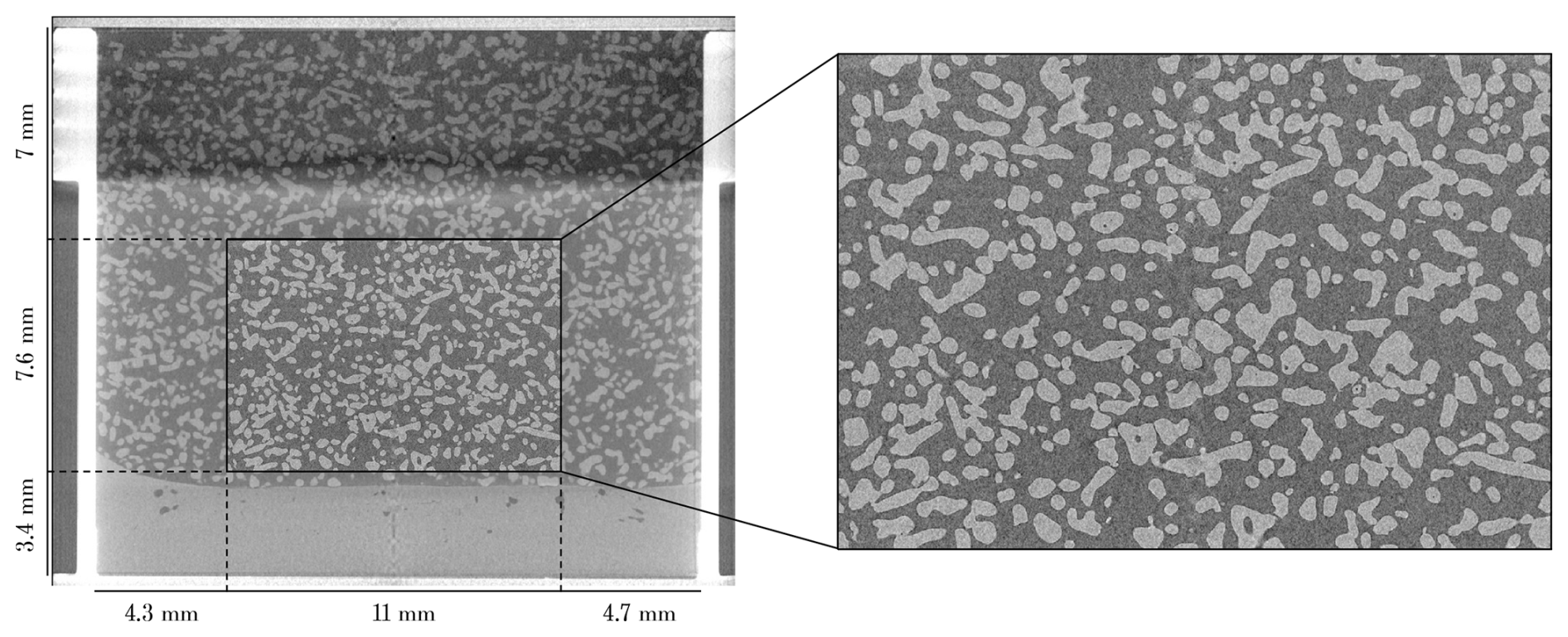
Figure 3 Reconstructed grey-scale vertical slice from a low resolution scan (left panel) and from a high resolution scan (right panel) of a sample RGd at the first time step of an experiment. Light grey shapes correspond to ice, and darker grey corresponds to air. On the left panel, the bright white parts correspond to the sample holder, and the ice layer is visible at the bottom of the snow.

For the HR scans, the X-ray source was set with a current of 132 µA, a tension of 60 kV with a small focal mode (about 5 µm focal spot size). 1440 projections were measured by the detector (127 µm pixel pitch, 1920 × 1536 pixels) during a 360° turn, with a frame rate of 1 image per second, and an averaging of two frames per image. The zoom was set to get a nominal voxel size of 8.5 µm. The obtained images correspond to sub-volumes of the snow samples and have, after reconstruction, a size of length × height × width = 11 × 7.6× 11 mm, as illustrated in Fig. 3. The image total volume of 919 mm³ was also chosen to be larger than the representative elementary volume (REV), defined as the minimum volume on which computed properties are representative of the whole snow sample under study, which has been found to be less than 63 mm³ for various properties (Kaempfer et al., 2005; Brzoska et al., 2008; Zermatten et al., 2011; Calonne et al., 2011). One HR scan lasted around 48 min.

For the LR scans, the X-ray source was set with a current of 200 µA, a tension of 80 kV with a medium focal mode (about 15 µm focal spot size). 1000 projections were measured by the detector during a 360° turn, with a frame rate of 5 images per second, and an averaging of three frames per image. The zoom was set to get a nominal voxel size of 25 µm. Three scans were stacked vertically to get the full volume without metal artifacts from top and bottom aluminum plates. The obtained images correspond to sub-volumes of the snow samples and have, after reconstruction, a size of length × height × width = 22.5 × 18.7 × 22.5 mm, as illustrated in Fig. 3. One LR scan lasted around 30 min.

Every 4 h, the following sequence was automatically initiated: first, the detector calibration (back and white calibration), then an HR scan at 8.5 µm resolution, and finally, an LR scan at 25 µm resolution. For one timeseries, i.e., for one 7 d experiment, about 40 HR scans and 40 LR scans were made.

3.2.2 Image processing and storage

After scanning, grey-scale 3D images were reconstructed from the projections at each scan, using the filtered back projection algorithm with the X-Act software. Center-shift and ring artifact corrections were applied to ensure accurate reconstruction.

The next step was the registration of the grey-scale 3D images. Despite setting the same x-, y-, and z-positions for each scan, small spatial differences between scans of the same time series were found and needed to be corrected. To spatially realign each image of a time series, the 3D images were compared from one time step to another and readjusted to get the best grey-scale matching. First, the LR images were registered by using the sample holder as a reference. Then the HR scans are readjusted by matching them with their respective LR images. Registration is conducted with micrometric accuracy. Figure 3 shows an HR scan that is overlaid on its corresponding LR scan. The registered 3D images were aggregated to get a 4D data set for each time series.

Finally, the HR 4D data sets were segmented into a binary data set (0 for air, 1 for ice) NumPy-like array. We adapted the segmentation algorithm from (Hagenmuller et al., 2013; Boykov and Funka-Lea, 2006), which is based on minimizing the segmentation energy, to 4D data. Here, the time series is treated as a whole (and not a series of independent 3D scans), which enables consistent segmentation in time. The energy-based segmentation finds the segmentation that minimizes an energy composed of energy related to the log-likelihood of being of one phase knowing the local grey-scale value and an interface energy, which is the air-ice 4D surface area times a smoothing factor r. A simple thresholding would correspond to r=0, increasing r smooths the interface. Here, the smoothing factor r was set to 5 for all series.

4D data are saved in a .zarr format, version 2. This data format is convenient for storing multidimensional data. It divides the saved data into subsets referred to as chunks, which allows for easy parallel computation. Zarr files are accessible from various code languages, including Python, C, C$++$, Rust, Javascript, Java, and Julia (https://zarr.dev/, last access: 9 April 2026). We chose this format for its simplicity of usage, parallel computation, and content compressibility. The whole data set takes 150 GB of storage. 4D data are accompanied by a readme.txt file with an example of Python code to open and visualize the data.

3.2.3 Geometrical property computations

Snow density and SSA were used to characterize the initial snow samples (Sect. 3.1). Density was calculated using a simple voxel counting method, while surface area was calculated using the Crofton approach described in Lehmann and Legland (2012). This method is based on the Cauchy-Crofton formula, which explicitly relates the surface area to the number of intersections with any straight lines in a 3D volume. Its high accuracy compared to other area computation methods for various images was assessed by Hagenmuller et al. (2016). In Sect. 4, the grain's shape is highlighted using the surface mean curvature. At a given point of the 3D image, two principal curvatures can be calculated: a maximal curvature κ₁ and a minimal curvature κ₂. From these two curvatures, the mean curvature H can be calculated:

$$\begin{array}{}\text{(1)}& H={\displaystyle \frac{\mathrm{1}}{\mathrm{2}}}({\mathit{\kappa }}_{\mathrm{1}}+{\mathit{\kappa }}_{\mathrm{2}})\end{array}$$

We used the open-source library DGtal to compute the curvatures on discrete surfaces of our 3D binary images, based on the theoretical work of Lachaud et al. (2022).

4 Time-series images of dry snow metamorphism

We provide a 4D data set of 20 experiments on dry snow metamorphism, with a temporal resolution of 4 h and a spatial resolution of 8.5 µm, and with systematic changes in experimental conditions. Videos showing the temporal evolution of the microstructure are also available for each experiment (repository link available in Sect. 5). To illustrate the data set, we present visualizations of snow microstructures obtained from the experiments (Figs. 4, 5, 6, 7, and 8). In what follows, the presented images are not the full snow images but cropped volumes. They consist of vertical slices of dimension length × height × width = 1300 × 900 × 100 voxels, or 11 × 7.65 × 0.85 mm. To emphasize the grain's shape, the microstructure is shown in terms of mean curvature, with values ranging from −20 to 20 mm⁻¹. Thus, in the following figures, convex or saddle surfaces appear in red, concave or saddle surfaces appear in blue, and flat surfaces appear in grey. Note that, at the image boundaries, artificial surfaces are created where ice grains are cut; these surfaces are flat and appear in grey, but they should not be considered as real surfaces of the snow microstructures. Hereinafter, grain shape and size are estimated qualitatively.

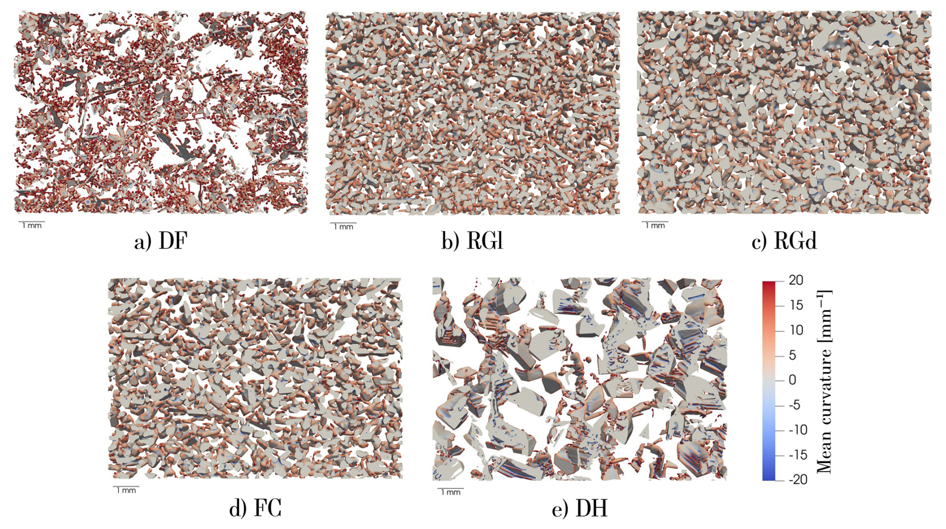
Figure 4 Images of the five initial snow sample types used in this study. To facilitate the visualization, a section of only 0.85 mm thickness is shown. Colors correspond to the surface mean curvature. Sample names are described in Sect. 3.1.

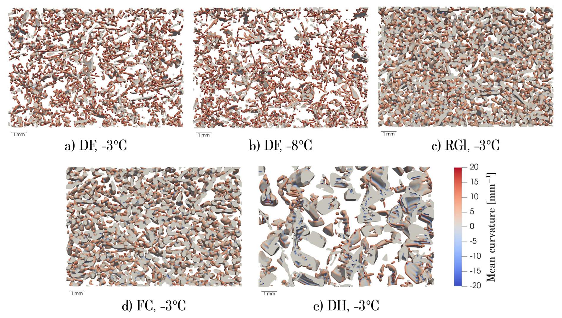
Figure 5 Images of the snow samples obtained after one week of equi-temperature conditions (final images). To facilitate the visualization, a section of only 0.85 mm thickness is shown. Information on the initial sample type and temperature conditions is provided. Colors correspond to the surface mean curvature. Sample names are described in Sect. 3.1.

4.1 Images of the initial snow sample types

First, Fig. 4 presents the 5 initial types of snow samples used for our experiments and described in Sect. 3.1. The figure highlights the large range of snow microstructure investigated. The mix of decomposing fragmented particles and rimed surfaces (towards graupel) is seen for the DF sample, with a mix of large, star-like or dendritic crystals and small, rounded pustules (Fig. 4a). Differences between the two types of rounded grains, samples RGl and RGd, can be assessed, notably in terms of density and grain size (Fig. 4b and c). The sample DH shows some typical depth hoar characteristics, with large cup-shaped grains oriented downward and striated surfaces (Fig. 4.e). This snow sample type exhibits the largest grain size of all initial snow types.

4.2 Images of equi-temperature metamorphism

Next, we illustrate the provided time series of equi-temperature metamorphism. The snow microstructures obtained at the end of these experiments are presented in Fig. 5. After one week in near-isothermal conditions, snow grains are overall more rounded, as they show lower extreme values of mean curvature compared to their initial state (Fig. 4). It is worth noting the evolution of the depth hoar sample: the size and general shape of the snow grains changed little, but on closer inspection, the striations and angles on the surface of the grains have become smoother from Figs. 4e to 5e. Videos available in Sect. 5 are more indicative of the grain's shape evolution happening during these equi-temperature metamorphism.

4.3 Images of temperature gradient metamorphism

Figure 6 shows the snow microstructures obtained at the end of the temperature gradient experiments. As an overview, the results of all 15 TGM experiments are presented and ordered in terms of the initial sample type, temperature gradient, and temperature. The impact of the temperature gradient is visible, as classically described in the literature (e.g. Colbeck, 1983): a gradient of 10 K m⁻¹ leads to the formation of faceted crystals (first column of Fig. 6), while a gradient of 40 or 100 K m⁻¹ leads to the formation of depth hoar (second and third columns of Fig. 6). The effect of temperature gradient magnitude on depth hoar shape is visible: the higher the temperature gradient, the larger the depth hoar. Videos available in Sect. 5 also show, especially for the DF sample, that the grain evolution at a temperature gradient of 100 K m⁻¹ is not similar to the grain evolution at a temperature gradient of 40 K m⁻¹. This highlights that there are discrepancies of shape within depth hoar depending on the temperature gradient magnitude, as shown in e.g. Akitaya (1974).

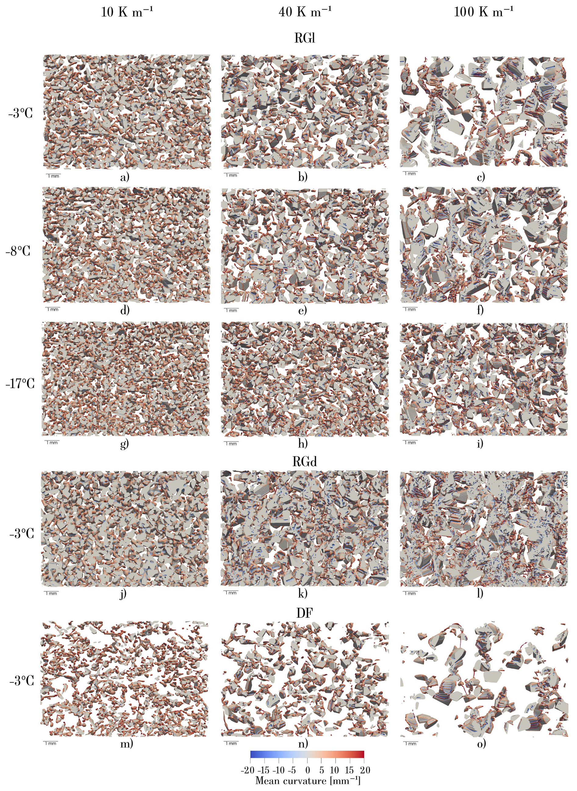
Figure 6 Images of the snow samples after one week of temperature gradient conditions (final images). A section of only 0.85 mm thickness is shown. The images are structured regarding the initial sample type, temperature gradient, and mean temperature. The sample names are described in Sect. 3.1. Colors correspond to the surface mean curvature.

The effect of the temperature on snow metamorphism can also be observed. For the same magnitude of temperature gradient, the temperatures at which the gradient occurs significantly impact the final snow microstructure: the lower the temperature, the slower the metamorphism and the recrystallization rate of the ice grains, as shown by previous studies (e.g. Kamata et al., 1999; Kaempfer and Schneebeli, 2007; Pinzer et al., 2012). The effect of the temperature is explained by the fact that the saturation vapor pressure in air increases exponentially with temperature. Hence, a given temperature gradient in snow induces a larger saturation vapor pressure gradient in warmer conditions compared to colder ones, and thus a higher metamorphism rate. In our data, this effect can be seen, for example, by comparing Fig. 6c, f, and i: smaller depth hoar and smaller pore spaces are obtained after a week of temperature gradient of 100 K m⁻¹ at a mean temperature of −17 °C compared to a mean temperature of −3 °C. Another example of the temperature effect is that the microstructure of the depth hoar obtained at a gradient of 100 K m⁻¹ at −17 °C (Fig. 6i) exhibits features that are more similar to the depth hoar obtained at a gradient of 40 K m⁻¹ at −8 °C (Fig. 6e) than the depth hoar obtained at a temperature gradient of 100 K m⁻¹ at −8 °C (Fig. 6f).

Finally, the effect of the initial sample type can be seen, as different depth hoar shapes are obtained from the different samples. Regarding snow density, we can compare the evolution of dense and light rounded grains in the same temperature conditions. Different types of depth hoar, with regard to the grain's shape and density, are obtained from the RGl and RGd samples for temperature gradients of 10, 40, and 100 K m⁻¹ at −3 °C. As shown by Akitaya (1974) and Pfeffer and Mrugala (2002), for dense snow, the growth of the grains is more constrained in space, due to the surrounding grains, than for snow with larger pore space, which influences the grain formation (Akitaya, 1974; Pfeffer and Mrugala, 2002). In line with this, the depth hoar formed from dense rounded grains at a gradient of 100 K m⁻¹ (Fig. 6l) can be considered as hard depth hoar (e.g. Akitaya, 1974; Bouvet et al., 2023).

4.4 Grain-to-grain evolution

Finally, we illustrate the provided time series and present the temporal evolution of the snow microstructure for the case of a temperature gradient of 100 K m⁻¹ in Figs. 7 and 8. Images at three consecutive time steps are shown. These figures illustrate the high temporal and spatial resolution of the time series combined with high precision registration, which allows tracking the evolution of the grain interfaces with time. By looking at the grain interfaces from one step to the other, one can see their evolution. For example, in Fig. 7, the cup shape visible in the middle clearly increases downwards, along the vertical direction, with more and more striations appearing inside the cup during the growth. In Fig. 8, the arms of the dendrite in the middle sublimate, while sharp angles start to appear on other grains.

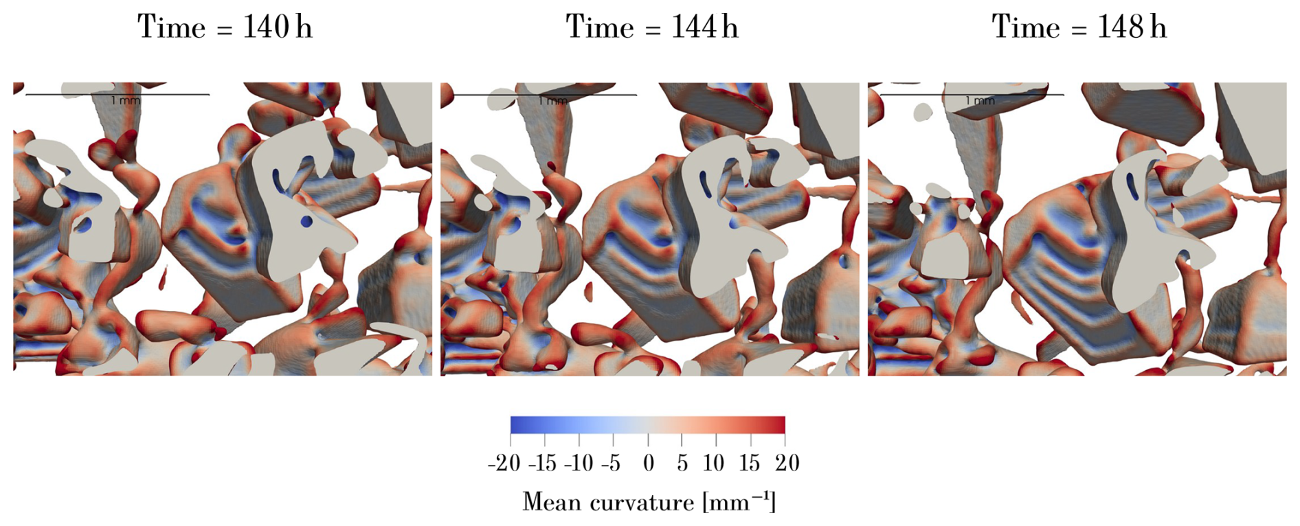
Figure 7 Temporal evolution of a RGl sample exposed to a temperature gradient of 100 K m⁻¹ at a mean temperature of −3 °C. To facilitate the visualization, a section of only 0.85 mm thickness is shown. Colors correspond to the surface mean curvature.

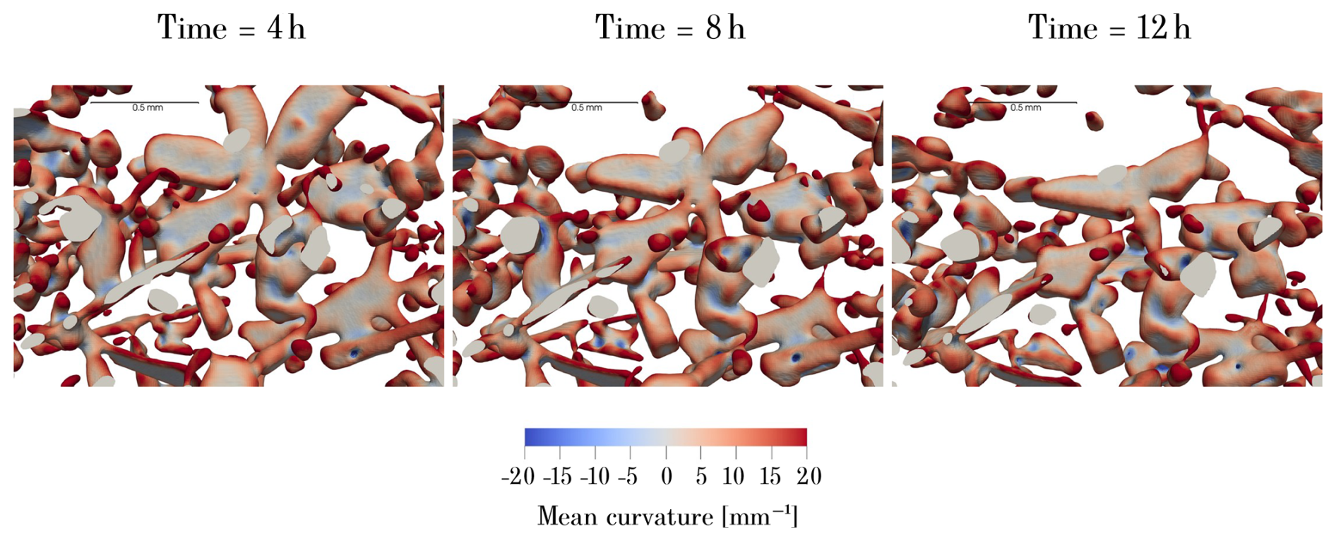
Figure 8 Temporal evolution of a DF sample exposed to a temperature gradient of 100 K m⁻¹ at a mean temperature of −3 °C. To facilitate the visualization, a section of only 0.85 mm thickness is shown. Colors correspond to the surface mean curvature.

5 Data availability

The 4D data set presented in this paper, along with videos showing the evolution of the microstructure, are available on Pangaea (https://doi.org/10.1594/PANGAEA.992556, Dick et al., 2026). Videos are also available on YouTube (https://www.youtube.com/@Snow-Science, last access: 9 April 2026).

6 Conclusions

This study provides time series of 3D images of snow microstructure for 20 scenarios of dry snow metamorphism. Videos of these time series are also provided. This data set comes from 20 experiments in which the evolution of centimetric snow samples was monitored by tomography with a frequency of 4 h and a spatial resolution of 8.5 µm during 7 d. For that, a new metamorphism cell, called CellCold, was developed and allows controlling thermal boundary conditions on the snow sample continuously, including during scanning. We used five types of initial snow samples, which include decomposed and fragmented particles, light rounded grains, dense rounded grains, faceted crystals, and depth hoar. Different temperature conditions were applied, exploring temperature gradients from 0 to 100 K m⁻¹ and mean temperatures of −3, −8, and −17 °C.

Two types of data are made available: 4D data in .zarr format consisting in time series of binary 3D images of snow microstructure, together with the metadata, as well as videos in format .mp4 showing the temporal evolution of snow during the experiments, using the surface mean curvature to highlight the grain features (repository links are available in Sect. 5). Both data sets are accompanied by a readme.txt file with explanations on the data organization and an example of Python code to read and visualize the 4D .zarr data. Videos are also available on YouTube, with the link provided in Sect. 5.

This data set opens new opportunities to improve the understanding of dry snow metamorphism and its modeling. Systematic variations in the control parameters allow separation of each parameter's impact on the temporal evolution of the snow microstructure. Geometrical properties of the microstructure can be calculated with high precision due to the images' high spatial resolution. In addition, the high temporal resolution of the experiments offers the possibility to track the interface velocity during different snow metamorphism.

Appendix A

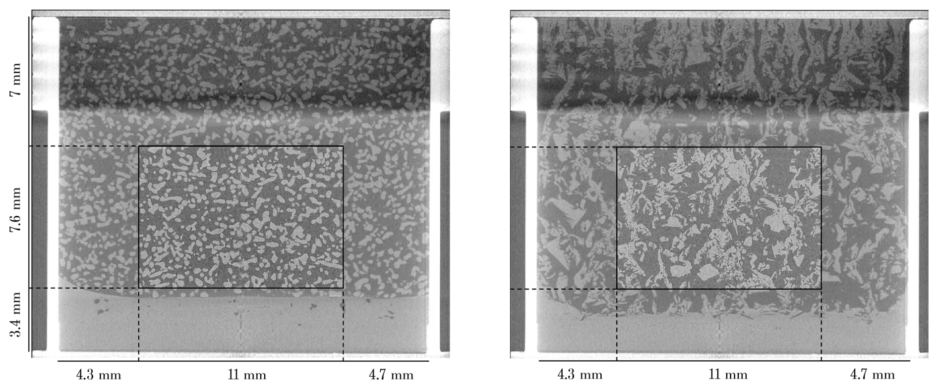
Figure A1 Reconstructed grey-scale vertical slices from the low resolution scans of a sample RGd exposed to a temperature gradient of 100 K m⁻¹ at −3 °C. The corresponding high resolution scans are shown in the middle. The left panel corresponds to the first time step, the right panel corresponds to the last one, after 164 h. Light grey shapes correspond to ice, while darker grey shapes correspond to air, and the bright white parts correspond to the sample holder. The ice layer is visible at the bottom of the snow.