Soil information and soil property maps for the Kurdistan region, Dohuk governorate (Iraq)

We present the first detailed soil property maps at multiple depths for the northwestern autonomous Kurdistan region of Iraq (Dohuk). A total of 532 soil samples from 122 sites were collected at five depth increments (0–10, 10–30, 30–50, 50–70, and 70–100 cm), and their mid-infrared (MIR) spectra were measured. A subset of 108 samples, selected via Kennard–Stone sampling, was analysed in a laboratory on ten soil properties. A Cubist model was trained and used from these measured values to predict all samples' soil properties from their MIR spectra. Digital soil mapping was conducted using a machine learning regression techniques based on a quantile random forest model, trained on the predicted soil properties and using a total of 85 covariates at 30 m pixel resolution, resulting in 50 prediction maps in total. Results were compared with the SoilGrids 2.0 product and a regional texture model. Soil depth was also mapped using a similar model with 26 covariates. Our model outperformed global SoilGrids 2.0 predictions in resolution and accuracy, with texture RMSEs (sand: $\stackrel{\mathrm{‾}}{x}$ RMSE 11.03; silt: $\stackrel{\mathrm{‾}}{x}$ RMSE 8.82; clay: $\stackrel{\mathrm{‾}}{x}$ RMSE 7.39) comparable to local models. Key predictors included Landsat 8 SWIR, EVI, SAVI, Sentinel 2 SWIR, PET and solar radiation. Spatial patterns reflected the contrast between the flat areas of the Selevani and Zakho plains, as opposed to the shallower and steeper Little Khabur Valley and anticline formations. Furthermore, the soil depth prediction model (R² 0.39; RMSE 30.76 cm) showed strong correlation with slope and a similar pattern distribution with deeper soils in the flat areas of the Selevani and Zakho plains, while shallow soils were predicted in the anticline and strongly erodible areas. Our comprehensive dataset (https://doi.org/10.1594/PANGAEA.973700, Bellat et al., 2024a; https://doi.org/10.1594/PANGAEA.973701, Bellat et al., 2024b; https://doi.org/10.1594/PANGAEA.973714, Bellat et al., 2024c; https://doi.org/10.6084/m9.figshare.31320958.v2, Bellat et al., 2026a; https://doi.org/10.57754/FDAT.d5h1h-4x027, Bellat et al., 2026b) offers substantial insights for soil knowledge in the region, as well as for aridic and semi-aridic areas.

1 Introduction

Soils record chemical, physical and biological processes over extended temporal scales (Hillel and Hatfield, 2005; Schaetzl and Anderson, 2005; Duchaufour et al., 2020). They are part of global exchanges (Bossio et al., 2020; Lal et al., 2021; Telo da Gama, 2023) and exert significant influence on local ecosystems (Adhikari and Hartemink, 2016; Scholten et al., 2017; Zeraatpisheh et al., 2022; Webber et al., 2023; Guan et al., 2024). Soil texture provides insights into soil stability, water retention, carbon storage, and biomass production (Rabot et al., 2018), while pH regulates soil acidity and nutrient availability for plants (Thomas, 1996; Neina, 2019). Organic carbon (OC) reflects local organic production and functions as a major carbon sink for CO₂ at a global level (Trivedi et al., 2018; Bossio et al., 2020; Beillouin et al., 2023). Inorganic carbon – calculated as total carbon (C_t) minus organic carbon – also plays a critical role in carbon sequestration in semi-arid zones (Zamanian et al., 2016; Sharififar et al., 2023). Calcium carbonate (CaCO₃), abundant in calcareous soils of semi-arid climates, further influences both acidity (Yu et al., 2023) and carbon dynamics (Umer et al., 2020; Dou et al., 2023). Additional key soil properties include total nitrogen (N_t), which influences plant growth (Crawford and Forde, 2002; Anas et al., 2020), and electrical conductivity (EC), essential for assessing soil water content or capacity (Brevik et al., 2006), and soil salinity (Friedman, 2005), particularly problematic in arid and semi-arid regions such as Iraq (Smith and Robertson, 1962; Christen and Saliem, 2013; Azeez and Rahimi, 2017). Evaluating all of these properties and establishing a taxonomic classification of a soil gives information on its ability to fit agricultural purposes and helps to better understand the development of soils over time and under changing climatic conditions.

In the Dohuk Governorate (Parêzgeha Dihok) of north-western Kurdistan region of Iraq (Herêmî Kurdistan, Fig. 1), exploratory mapping efforts (Buringh, 1957, 1960; Altaie, 1968; Altaie et al., 1969; Barzanji, 1973; Muhaimeed et al., 2014; Muhaimeed, 2020) identified the presence of semi-arid and mountainous soils shaped by complex interactions between geomorphology, parent material and climate. The fluvial dynamics of the Tigris River (Dîcle) have been recognised as a major factor in landscape formation, influencing salinity, clay deposition, and vertic properties through sedimentation and erosion (Buringh, 1960, pp. 51–54). However, critics (Wilkinson, 1990) have suggested that vertic features and horizons might have been overestimated (Buringh, 1957, 1960; Altaie, 1968; Abdulrahman et al., 2020). Gypsum is another critical factor in local soil development, either inherited from primary deposits such as alabaster formations (Buringh, 1960, p. 106), or formed secondarily through irrigation-induced precipitation and soil chemical processes (Buringh, 1960, p. 107). High gypsum concentrations are commonly found in areas south and south-west of the Zagros and Taurus mountain chains (Smith and Robertson, 1962; Barzanji, 1973; Azeez and Rahimi, 2017), reflecting the influence of regional hydrogeology, and aquitard structures (Buringh, 1960, p. 108; Azeez and Rahimi, 2017). Favourable factors for soil development have been poorly explored outside of the alluvial plain area (Altaie et al., 1969; Barzanji, 1973). While some valley bottom soils may exhibit higher organic carbon content (Buringh, 1960, p. 78; Altaie, 1968) soils in upland areas are generally poorly developed due to severe erosion, leading to shallow, fragmented profiles (Muhaimeed et al., 2013) referred to as “broken soils” (Buringh, 1957; Altaie, 1968).

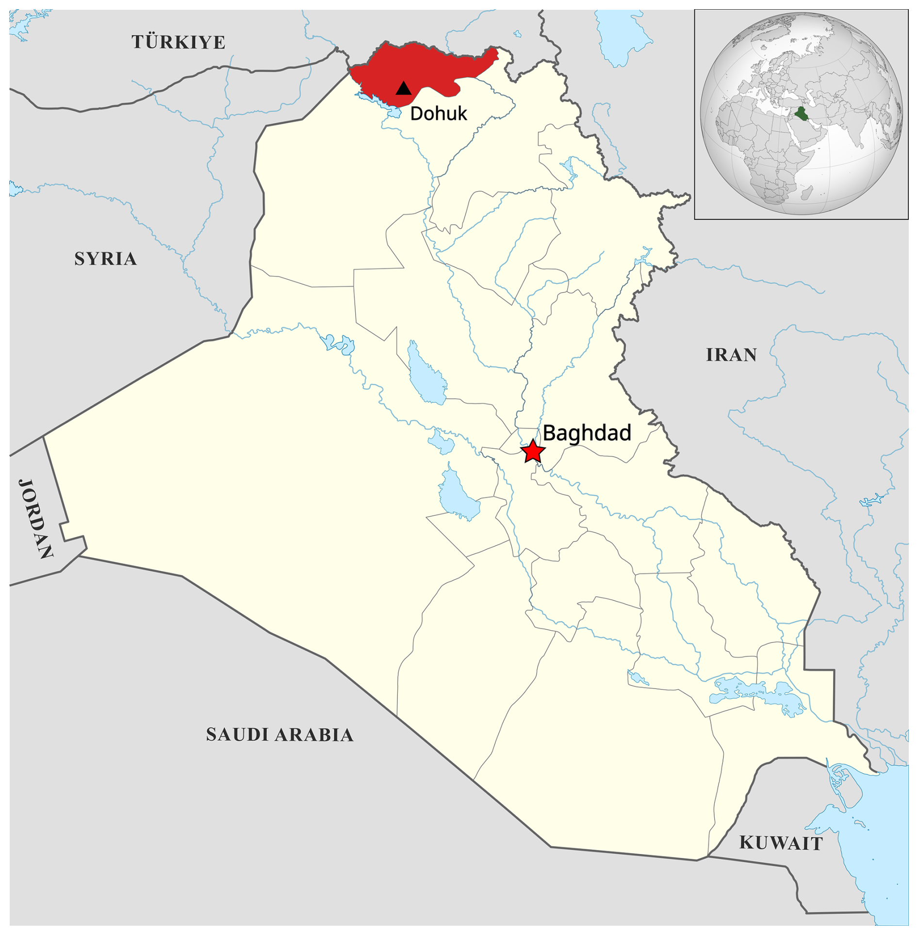
Figure 1 Location of Dohuk governorat in the Republic of Iraq (Wikimedia commons). Realised with QGIS 3.34.5.

Quantitative soil property data for the region remain scarce. The global SoilGrids 2.0 product (Poggio et al., 2021) offers coarse-resolution (250 m) predictions of key soil attributes. While adequate at a national scale in some regions (Varón-Ramírez et al., 2022; Shi et al., 2025), its performance at finer scales is limited, particularly due to sparse calibration points in the Middle East and Iraq (Batjes et al., 2020; FAO and IIASA, 2023). At the regional scale, only one recent study has attempted digital texture mapping (Yousif et al., 2023), but it covers a different area and does not account for the full range of soil-forming factors described in the scorpan model (McBratney et al., 2003).

Previous classifications and soil descriptions in the region were mostly carried out at the national scale and do not reflect recent landscape changes (Forti et al., 2022), nor do they align with contemporary standards (IUSS Working Group WRB, 2022). Moreover, no spatially explicit dataset currently exists for the most important chemical and physical soil attributes. While the previous mappings only used limited observations windows, with modern digital soil mapping (DSM), the spatial distribution of soils and their characteristics can now be described and modelled with increasing accuracy (Behrens and Scholten, 2006; Taghizadeh-Mehrjardi et al., 2014). Therefore, we have developed a meso-scale (1:200 000; 30 m pixel) DSM of key properties in the Dohuk region, alongside an updated classification based on the WRB taxonomy (IUSS Working Group WRB, 2022). Soil sampling campaigns conducted between 2022 and 2023 enabled the creation of 10 soil property maps across five depth intervals and a soil depth model for the western part of Dohuk governorate (Fig. 1). All data products follow the FAIR principles (Findable, Accessible, Interoperable, Reusable; Wilkinson et al., 2016) and were adapted to physical geography specificities (Bailo et al., 2020). These outputs are relevant for application in agriculture, geography, and ecology, especially as climate change exacerbates desertification in Iraq (Eltaif and Gharaibeh, 2022; Eltaif et al., 2024). The production of a spatial dataset from unexplored region, and the digital soil maps from recent field observations became an asset for depicting actual soil situations and exploring potential solutions.

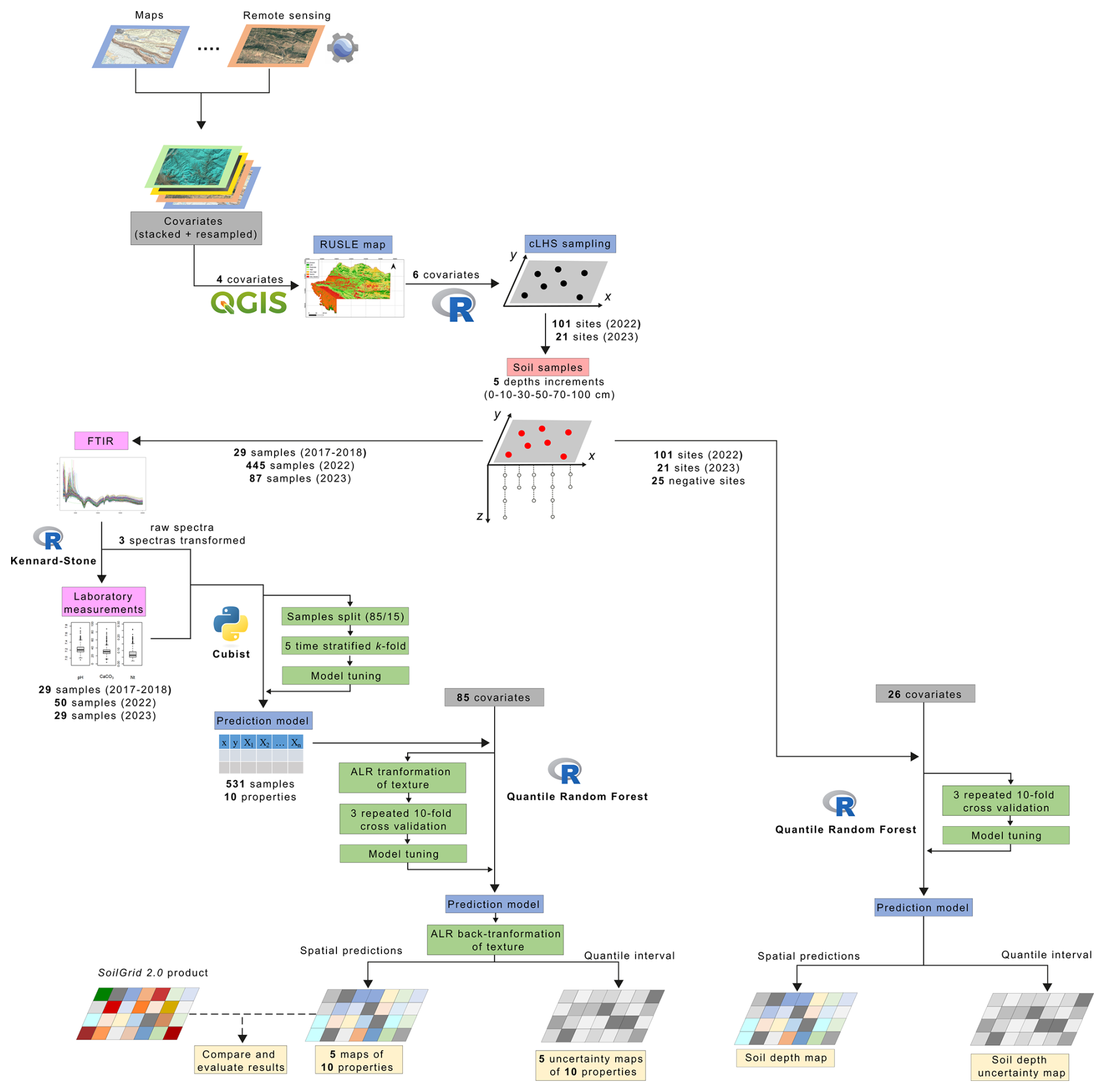
Figure 2 Workflow of the soil properties maps production based on Malone et al. (2022) protocol. Realised with Inkscape 1.4, and inspired by Shi et al. (2025) design.

2 Material and Methods

The workflow (Fig. 2) followed a semi-standardised fully reproducible protocol (Malone et al., 2022). Using a conditioned Latin hypercube sampling design (cLHS), 532 soil samples were collected from 122 sites (Table 1) and analysed via mid-infrared (MIR) spectroscopy. A representative subset of 108 samples, including legacy material from older surveys, underwent laboratory analysis for detailed physical, biological, and chemical characterisation. These samples were used to calibrate a Cubist regression model, with one raw and three transformed MIR spectra as predictor variables. The resulting predictions of soil properties were then integrated into a digital soil mapping framework (Lagacherie et al., 2006; Behrens and Scholten, 2006; Brevik et al., 2016; Malone et al., 2017; Hengl and MacMillan, 2019), following the scorpan equation model (Eq. 1; McBratney et al., 2003), and computed with a quantile random forest regression for each of five soil depth increments. Additionally, a soil depth map was developed using a similar model, incorporating remote sensing covariates and field observations. The digital soil maps integrate field observations and spatial predictions derived from a suite of remote sensing and spatial datasets. All datasets used are listed in Table , with further methodological detail provided in the Supplement.

$$\begin{array}{}\text{(1)}& S_{\mathrm{a}}=f(s,c,o,r,p,a,n)\end{array}$$

2.1 Study area

The data were collected from the Dohuk governorate in the Kurdistan region of Iraq, specifically from the Simele (Qezaya Sêmêl) and Zakho districts (Qezaya Zaxo, Fig. 3) covering a total area of 2280 km². The region is often referred to as Eastern Khabur/ (Xabûr, Pfälzner and Sconzo, 2016), though it is sometimes divided into two entities: the eastern Syrian al-Jazira (Ǧazīra) for the western and southern part and the mountain chain of Khabur for the northern part (Abdulsalam and Schlaich, 1988).

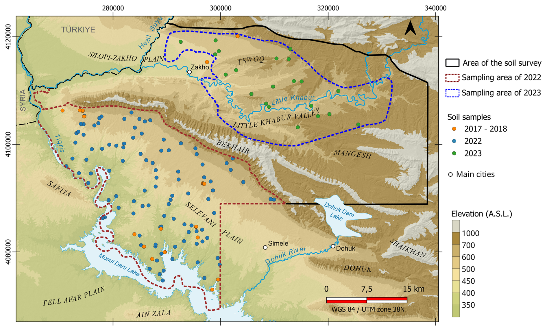
Figure 3 Map of the sampling areas and different sample locations (Background: Copernicus data ESA and Airbus, 2022). Realised with QGIS 3.34.5 and Inkscape 1.4.

2.1.1 Tectonic development and parent material

Our study area within the Dohuk governorate is located within the northwestern segment of the Zagros-fold thrust belt (ZFTB), a mountain belt that extends from southern Iran NW-ward to the Kurdistan Region of Iraq and SE Turkey. The ZFTB resulted from the ongoing convergence between the Arabian and Eurasian plates (Berberian, 1995; Agard et al., 2011; Mouthereau et al., 2012; Sembroni et al., 2024). The convergence started in the late Cretaceous with the subduction of the Neotethys oceanic crust beneath the Eurasia Plate and the obduction of the ophiolite sequences on Arabia's margin, followed by the subsequent continent-continent collision between the Arabian and Eurasian plates during the Oligocene-Early Miocene (Agard et al., 2011; Khadivi et al., 2012; Mouthereau et al., 2012; Koshnaw et al., 2017). Since the onset of continental deformation on the northeastern margin of the Arabian Plate (including the study area), it has propagated for 250–350 km (Blanc et al., 2003; Molinaro et al., 2005; Alavi, 2007; Agard et al., 2011; Mouthereau et al., 2012; Koshnaw et al., 2020; Zebari et al., 2020; Sembroni et al., 2024). Within the external part of the ZFTB, these zones include the Imbricated Zone, the High Folded Zone, and the Foothill (Low Folded) Zone (Berberian, 1995; Jassim and Goff, 2006; Fouad, 2012, 2014; Zebari et al., 2020).

The study area covers parts of the High Folded and Foothill zones (Fig. 4), where structures are mainly trending in a nearly E–W direction (Forti et al., 2021; Doski and McClay, 2022). The Bekhair/Ǧebel Bihair Anticline ( Bixêr) is the main structural and morphological feature in the area and plunges at the western end of our study area. It separates the Selevani Plain ( Selevani), which stretches from the northern bank of the Mosul Dam Lake to the anticline, in the south, from the Zakho-Cizre-Silopi Plain – later shorten into Zakho Plain – and Little Khabur Valley to the north (Forti et al., 2021; Doski and McClay, 2022).

The exposed rocks in the area include sedimentary units ranging in age from the Upper Cretaceous to the Pliocene (Sissakian and Al-Jiburi, 2012, 2014; Doski and McClay, 2022). The Upper Cretaceous units consist of platform carbonates and siliciclastic rocks (Jassim and Goff, 2006; Aqrawi et al., 2010). The Paleocene-Eocene units consist mainly of marginal marine marls and shales that interfinger with rigid carbonate units, followed by red Eocene clays and carbonates. These Upper Cretaceous-Eocene units are exposed within the anticlinal structures in the area. The Oligocene units are missing in the area; thus, the Eocene carbonates underlie the Middle Miocene clays, evaporites, and limestones. The Upper Miocene–Pliocene units consist of fluvial sandy succession, clay, and conglomerate deposited in the Zagros foreland basin (Jassim and Goff, 2006; Aqrawi et al., 2010). The Miocene-Pliocene units are exposed within the synclines and low-elevation area to the north and south of Bekhair Anticline.

The Quaternary deposits cover three different environments of the study area (Fig. 4). First, the flat area of the Selevani Plain and north of the Zakho Plain (Türkiye) is covered by residual clayey soil material, coming from the erosion of the Bekhair and Zagros anticlines. Second, along the riverbanks of the Tigris and Little Khabur rivers, sand and gravel-sized terrace deposits, as well as floodplain sediments of fine sand and clay, can be observed. Finally, Quaternary formations from alluvial fan sediments of clayey soil, combined with rock fragments coming from colluvial deposits, are visible in the foothills of the Bekhair and the shallow Little Khabur Valley. Sometimes, calcrete is also developed within the these Quaternary deposits (Sissakian and Al-Jiburi, 2012, 2014; Forti et al., 2021).

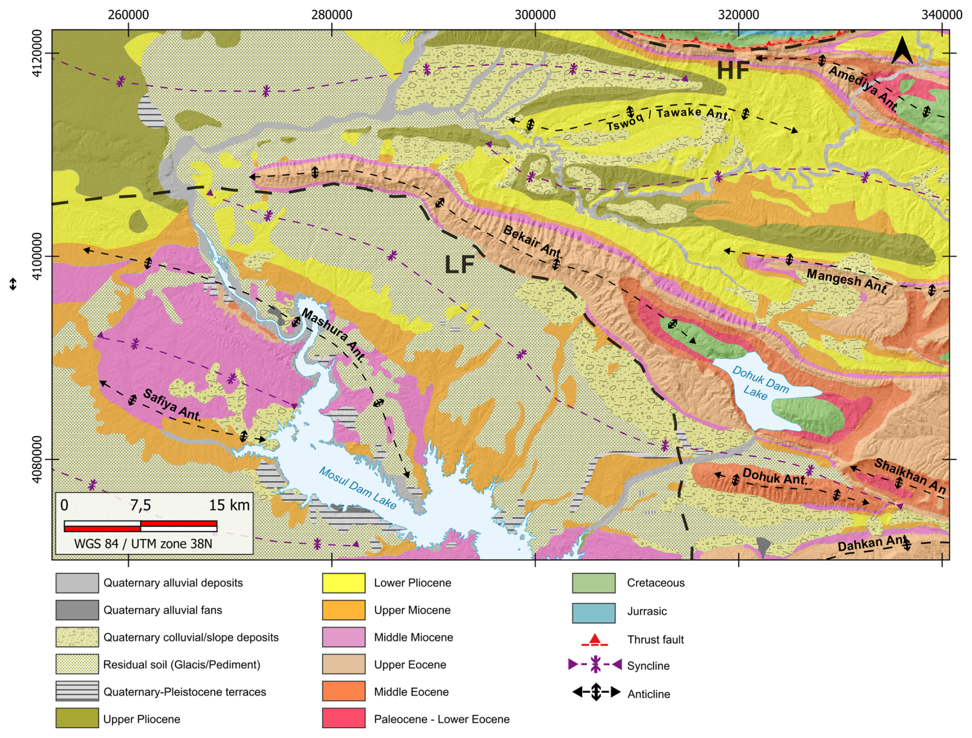
Figure 4 Geological map of the studied area compiled from: Ponikarov and Mikhailov (1986), Sissakian et al. (1995), Isiker et al. (2002), Al-Mousawi et al. (2007), Sissakian and Al-Jiburi (2012), Sissakian and Al-Jiburi (2014) and Doski and McClay (2022) (LF = Low-folded zone; HF = High-folded zone). Realised with QGIS 3.34.5 and Inkscape 1.4.

2.1.2 Climate and vegetation

The central part of the study area falls within a Csa (Hot-summer Mediterranean) agro-climatic zone, according to the Köppen Geiger classification (Köppen, 1936; Beck et al., 2018; Alwan et al., 2019). Annual precipitation ranges from 200 to 500 mm, with an average yearly temperature exceeding 16 °C (Fick and Hijmans, 2017; Salman et al., 2019; Najmaldin, 2023). Only the Little Khabur Valley, located north of the Bekhair anticline, experiences slightly cooler winters and receives higher rainfall, typically between 500 and 800 mm per year (Fick and Hijmans, 2017; Alwan et al., 2019). South of the Bekhair anticline, the Selevani Plain belongs to the Mesopotamian steppe floral complex, which supports a limited number of xerophytic shrubs and herbs, primarily Artemisia herba-alba mesopotamica often associated with Aristida plumosa (Guest and Al-Rawi, 1966, pp. 78–80; Zohary, 1973, p. 183). In contrast, the northern region, encompassing the Zakho Plain and Little Khabur Valley, falls within the Kurdo-Zagrosian climate zone, characterised by a denser xerophilous deciduous steppe forest, driven by its higher elevation and more favourable climatic conditions (Fig. B1; Guest and Al-Rawi, 1966, p. 68). Dominant shrubs include Anagyris foetida or Pistacia khinjuk are associated with trees as Quercus brantti, or Quercus boissieri, which grows between 800 and 1700 m of altitude. Historical records mention the presence of pine forests (Zohary, 1973, pp. 183–190), though they are likely no longer extant. In both the foothills of the Mesopotamian Plain and the Kurdo-Zagrosian space, cultivated Olivae europanis can be sporadically observed.

2.1.3 Geomorphology and soils

In the southern part of our study area, the Tigris floodplain and its Quaternary alluvial deposits have largely disappeared due to the construction of the Mosul Dam Lake (Forti et al., 2022). What remains are sporadic surface exposures of conglomerates and marls (Fig. B2; Forti et al., 2021) and three to four terraces levels (Al-Dabbagh and Al-Naqib, 1991; Forti et al., 2021, 2022). North of the Tigris river, in the Selevani Plain, combined action of wind and irregular water action of $w\stackrel{\mathrm{‾}}{a}d\stackrel{\mathrm{‾}}{\mathit{ı}}s$, have led to the formation of gullies on this depositional glacis (Yacoub et al., 2012; Forti et al., 2021), shaping a badland landscape (Fig. 5B). The Bekhair anticline and its imbricated zone form a structurally homogenous ridge dominated by exposed limestone and sandstone formations (Fig. 4, Forti et al., 2021), which are subject to lift-up process and tectonic action. The foothills on both sides of the ridge, however, are subject to wind, water erosion, and gravitational processes, resulting in extensive colluvial deposits (Fig. 5C; Sissakian and Abdul Jab'bar, 2014; Sissakian et al., 2015). In the area of the Tswoq anticline and the Little Khabur Valley, the landscape is dominated by sandstone and conglomerate. Soil surface erosional process are less pronounced in the Little Khabur Valley region due to the protective effect of denser vegetation cover. The Zakho Plain, located within a synclinal structure (Fig. 4), is a flat alluvial area, also less affected by erosion.

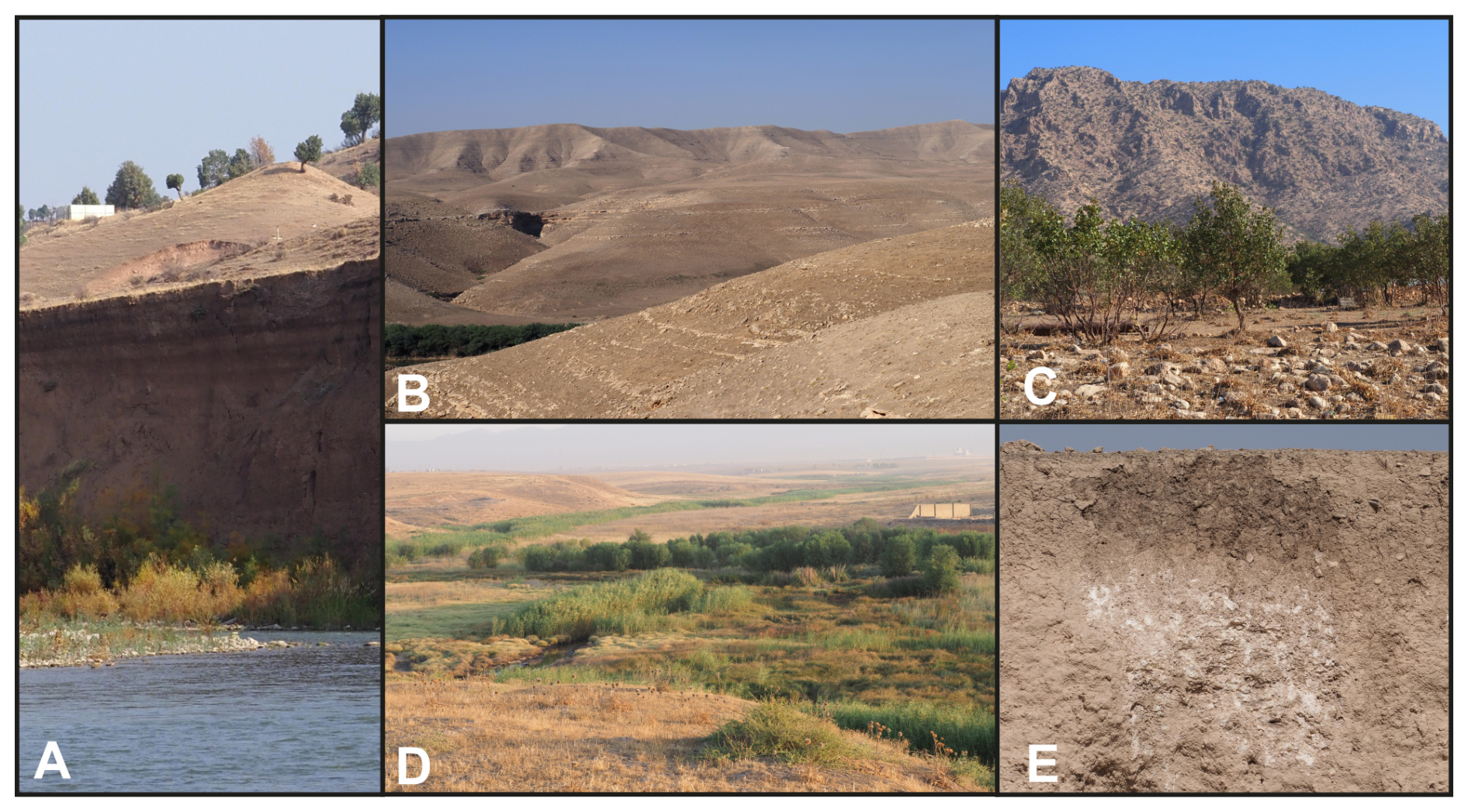
Figure 5 Examples of landscapes (A) Terraces of the Little Khabur (10–11 m) featuring a succession of colluvial and flood deposits. 37°05^′14.46^′′ N 42°56^′28.32^′′. (B) Hill and badland landscape on marl formation. $W\stackrel{\mathrm{‾}}{a}d\stackrel{\mathrm{‾}}{\mathit{ı}}s$ shape this landscape mainly used for grazing. 36°57^′16.86^′′ N 42°28^′38.53^′′ E. (C) Foothills landscape at the base of the Bekhair. Stones are visible on the surface, and olive trees (Olivae europanis) are cultivated in these foothills. Lithosols, Cambisols or Calcisols dominate this landscape. 37°03^′50.73^′′ N 42°34^′50.71^′′ E. (D) $W\stackrel{\mathrm{‾}}{a}d\stackrel{\mathrm{‾}}{\mathit{ı}}$ landscape with heavily developed vegetation, shrubs and small trees. Fluvisols or Vertisols are usually associated with this environment. 36°54^′35.33^′′ N 42°44^′29.64^′′ E. (E) Calcisol developed on a conglomerate formation formation. The top 10–15 cm shows an A humic horizon, followed by 5–10 cm of a Bt horizon and a C calcitic horizon at the bottom. 37°01^′24.61^′′ N 42°30^′37.11^′′ E. Realised with Inkscape 1.4.

Soil mapping in the region was initially carried out in the 1950s and 1960s as part of the Iraq soil mapping project (Buringh, 1957; Altaie, 1968; Altaie et al., 1969). We adapted Buringh's classification to the WRB system (IUSS Working Group WRB, 2022), improved spatial detail using modern satellite imagery (Sentinel 2 ESA, 2022; DEM ESA and Airbus, 2022; and Bing Maps https://www.bing.com/maps, last access: 6 September 2024), and completed the map with unrecorded Regosols and Fluvisols. This resulted in a new regional soil map built on an expert-based knowledge method (Fig. 6). The semi-arid climate, marked by sharp temperature variations and high subsurface CaCO₃ concentrations, has favoured the development of vertic and calcic features in many soil profiles (Abdulrahman et al., 2020). However, significant local variability exists. Soils adjacent to the Tigris River are typically calcic Vertisols, likely due to subsurface marl and conglomerate permeability. The Selevani Plain's glacis deposits are dominated by cambic and gypsic Calcisols (Figs. 5 and 6), with mediumly developed soil horizons, and a soil depth of 100 to 200 cm. North of the Selevani Plain, on the structural ridge and the steep slopes of the Bekhair anticline, soil development is minimal, due to active erosion, resulting in nudilithic Leptosols. On the northern side of the ridge, the Little Khabur Valley and its surroundings are dominated by poorly developed soil such as calcic Cambisols, Regosols and Leptosols, shaped by steep slopes and more erodible parent materials (conglomerate and sandstone), compared to the Simiele Plain. In contrast, the flat, irrigated Zakho alluvial plain, with higher precipitation, supports more developed soils, such as calcic isomeric Kastanozems (Fig. 6). Finally, Fluvisols occur sporadically along the Tigris and Little Khabur floodplains and major $w\stackrel{\mathrm{‾}}{a}d\stackrel{\mathrm{‾}}{\mathit{ı}}s$ channels riverbanks (Figs. 5 and 6), identifiable by their ochric and/or umbric horizons.

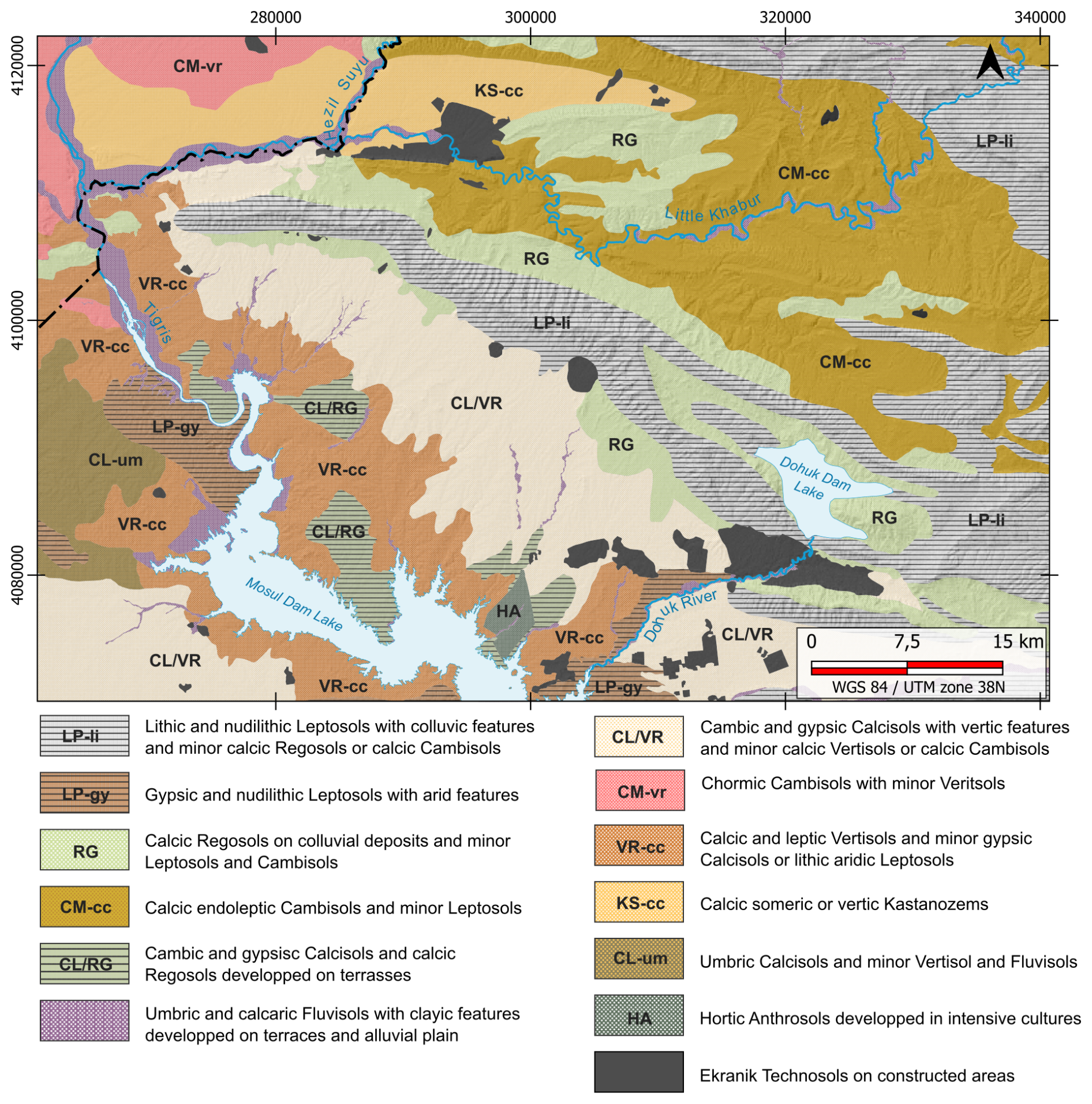
Figure 6 Soil type map based on the IUSS Working Group WRB (2022) classification. Observations come from survey informations and previous work of Buringh (1957), Altaie (1968) and European Soil Bureau Network and European Union (2005). Realised with QGIS 3.34.5 and Inkscape 1.4.

2.2 Sampling campaign

The 2022 campaign primarily focused on the Selevani Plain and the Tigris riverbanks, resulting in collecting at 101 sites a total of 445 samples. In 2023, the mission was conducted in the Zakho district, where 21 sites were visited and 87 samples were collected. Due to ongoing violence and conflict between the Kurdistan Workers’ Party (PKK) and the Turkish government in the mountainous areas of Zakho (Ertan, 2022), the 2023 survey coverage was reduced for safety reasons. To increase the number of training samples for model calibration (cf. Sect. 2.4.1), 16 additional sites and 29 samples were included from earlier 2017–2018 surveys, and were based on purposive, non-randomised sampling design. The total number of samples collected and analysed with the FTIR methods was 561 from 138 sites (Table 1).

Table 1 Sampling campaigns.

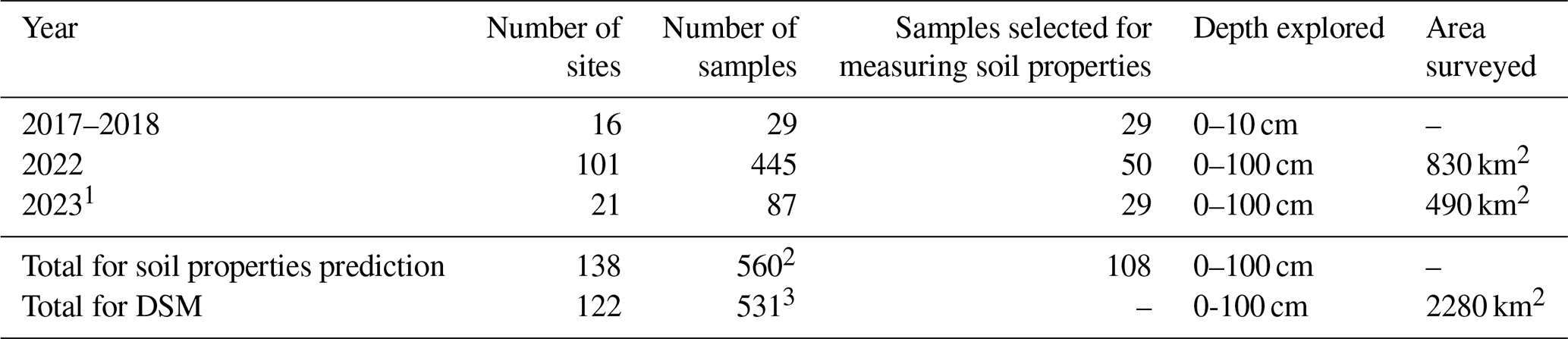
¹ Original size of the non-reduced area is 1450 km². ² One sample did have FTIR spectra out of range, and therefore was not used. ³ Samples of the 2017–2018 campaigns were not used for the DSM due to the absence of several depth increments, and the highly clustered locations near archeological sites with modified soil caracteristics.

2.2.1 Conditioned Latin hypercube sampling

Sampling design plays a critical role in ensuring that selected locations reflect the spatial and environmental variability of the study area (Brus, 2022). We adopted a conditioned Latin hypercube sampling (cLHS) approach, a method particularly suited to digital soil mapping applications (Minasny and McBratney, 2006; Stumpf et al., 2016). The cLHS method ensures that sampling points are distributed across the full range of values in selected environmental covariates by stratifying feature layers. For each covariate, a set of marginal strata is defined (intervals). The number of marginal strata for each covariate equals the sample size, resulting in pⁿ a total of marginal strata, where p is the number of covariates and n is the sample (Brus, 2022). Sampling was performed with R 4.4.0 (R Core Team, 2024) using the clhs package (Roudier, 2021).

We selected six covariates (Table ) which represent a broad range of parameters influencing soil variability. These included physical characteristics, underlying geomorphological formations (Forti et al., 2021), potential soil properties and erosion process.

The potential soil properties layer was constructed using spectral indexes (clay minerals, ferrous minerals, rock outcrop, carbonate) derived from climatic and satellite datasets (Copernicus, 2019; EROS, 2020). Erosion risk was modelled using the Revised Universal Soil Loss Equation (RUSLE; Renard et al., 1991), incorporating five key factor: soil erodibility (K), soil coverage (C), topographic effect (LS), rainfall-runoff (R) and erosion control practices (P; Cossart et al., 2020; Thapa, 2020; Abdi et al., 2023; Mehri et al., 2024). In our RUSLE model (Table C1), we set K as the soil strength factor based on texture and organic carbon values (Kouli et al., 2009), and C was set with values from Morgan (2005) and Swarnkar et al. (2018). Slope length and steepness factor LS were based on Desmet and Govers' method (Desmet and Govers, 1996), while the R factor from Morgan et al. (1984) was used. Finally, the conservation factor P, which could not be observed, has been set to 1 artificially, as suggested by Mehri et al. (2024).

2.2.2 Field measurements

At each site, samples were collected for the top 50 cm using a 3.5 cm ø auger and from depths up to 100 cm with a 2 cm ø auger. The different soil horizons' depths were measured, and colour was determined according to the Munsell soil colour chart. Samples were collected at five depth increments: 0–10, 10–30, 30–50, 50–70 and 70–100 cm. Bulk density was calculated for the topsoil using a 5.3 cm ø ring (Blake and Hartge, 1986). After removing the surface litter and loose sand, the sampling ring was used on the 0–10 cm soil layer. All samples were air-dried at 40 °C for 48 h before sieving at 2 mm for subsequent analysis.

2.3 Laboratory analysis

2.3.1 Mid-infrared spectroscopy

Mid-infrared spectroscopy to measure physical and chemical soil properties has significantly evolved over the past decades (Ng et al., 2022a) and offers reliable results while saving time and resources (Stenberg et al., 2010; Viscarra Rossel et al., 2022). All the 561 soils samples were ground under 1 µm with a Pulverisette 5/4, classic line (Fritsh, Idar-Oberstein, Germany) before being pressed into a tablet, mixing 1–1.3 mg of soil and 250 mg of potassium bromide (KBr). The spectra were analysed with a Vertex 80v (Bruker OPTIK GmbH, Germany), with a 4 cm⁻¹ resolution, on the 375–4500 cm⁻¹ interval.

The spectra were imported into R 4.4.0 and analysed using the prospectr (Stevens and Ramirez-Lopez, 2014) and simplerspec (Bauman, 2023) packages. To reduce noise interference, we decided to remove the measurements between 375–499 and 2451–2500 cm⁻¹ intervals and spectra value higher than 2 and lower than −2 (Curran et al., 1996; Ng et al., 2018). One sample was therefore removed due to its low values (< −2). The remaining 560 soil spectra were enhanced by applying three spectral transformations (Ng et al., 2018; Wadoux et al., 2021b; Ludwig et al., 2023), Savitzky-Golay with a polynomial order of 2 and a window size of 11 (SG 2.11), a moving average of 11 and standard normal variate transformation on the SG transformed spectra (SNV-SG). A total of 108 samples were selected for laboratory measurements (Table 2) using Kennard-Stone sampling (Kennard and Stone, 1969), ensuring a high diversity and variability of individuals, based on their spectral data (Ramirez-Lopez et al., 2014).

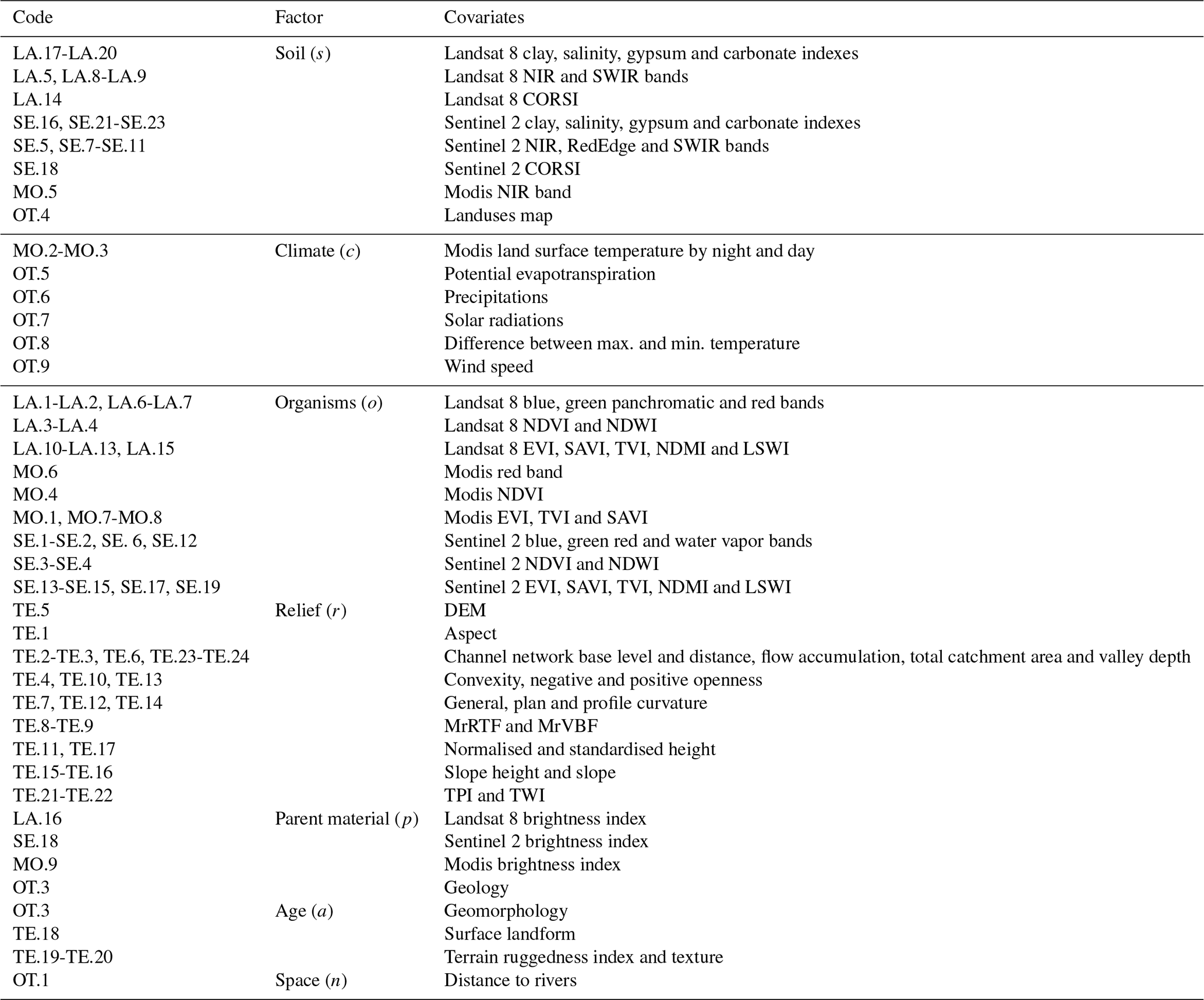
Table 2 Environmental covariates by soil forming factor, for the digital soil mapping. These factors are based on scorpan model (Eq. 1; McBratney et al., 2003; NIR = Near-infrared; NDVI = Normalised difference vegetation index; SWIR = Short wavelength infrared; EVI = Enhanced vegetation index; SAVI = Soil adjusted vegetation index; NDMI = Normalised difference moisture index; CORSI = Combined spectral response index; LST = Land surface temperature; TVI = Transformed vegetation index; LSWI = Land surface water index; DEM = Digital elevation model; MrRTF = Multiresolution index of the ridge top flatness; MrVBF = Multiresolution index of the valley bottom flatness; TPI = Topographic position index; TWI = Topographic wetness index).

2.3.2 Soil properties

On these 108 selected samples, seven properties were measured: pH, CaCO₃, N_t, C_t, OC, EC and texture. The pH was measured using a potassium chloride (KCl) solution, with a ProfiLine pH 3310 and a WTW SenTix 81 pH electrode (Fisher Scientific, Strasbourg, France). Carbonate calcium (CaCO₃) content was determined as a percentage using a calcimeter 08.33 (Royal Eijkelkamp, Giesbeek, Netherlands). Total nitrogen (N_t), total carbon (C_t) and total organic carbon (OC) were quantified as percentages with a CNS analyser, Vario EL III (Elementar, Hanau, Germany). The electro-conductivity (EC) was measured in micro-siemens per centimeter (µS cm⁻¹) using a Cond 330i/340i (WTW, Weilheim in Oberbayern, Germany). Texture property was determined as a percentage and measured through wet sieving for sand fraction and a SediGraph III for finer fractions (Micromeritics, Norcross, USA). Additionally, we estimated the mean weight diameter in mm (MWD, Eq. 2) based on the texture results.

$$\begin{array}{}\text{(2)}& \mathrm{MWD}=X_i\times W_i/\mathrm{100}\end{array}$$

where X_i is the mean diameter of i size fraction, and W_i is the weight percentage of i size fraction.

2.4 Models and pre-process

2.4.1 Spectra prediction

The Cubist model is a regression-based machine learning algorithm that extends the ideas of decision trees by combining rule-based predictive models with linear models at the leaves, enhancing both interpretability and predictive accuracy (Quinlan, 1992). This model excels at handling both continuous and categorical data, providing robust predictions even in the presence of complex interactions and non-linear relationships (Kuhn and Quinlan, 2024). Cubist’s strength lies in its ability to partition the data space and fit separate linear models to each segment, making it particularly effective for problems with distinct patterns or heteroscedasticity (Wang and Witten, 1996). This model has been applied in a variety of studies for soil property prediction from spectral predictors, such as Viscarra Rossel et al. (2016), Padarian et al. (2020), and Behrens et al. (2022). We tested a Cubist regression model on the four spectral datasets from each of our 560 samples in a Python (Python Software Foundation, 2022) environment using the Cubist library (Aselin, 2024). The model used a stratified 5-folds cross-validation and a tuned grid (n rules: 20, 30, 40 and n committees: 5, 10, 15).

2.4.2 Digital soil properties mapping

We based our soil property model on the soil formation factors of the scorpan equation (Eq. 1) developed by McBratney et al. (2003). We included 85 covariates (Tables 2 and ). The remote sensing variables were accessed through an API of Google Earth Engine (https://earthengine.google.com, last access: 15 January 2026) on Python, via the ee library (Google, 2025), and the different indices computed in R with the terra package (Hijmans et al., 2025). The terrain variables were computed on SAGA GIS 9.3.1 (Conrad et al., 2015) based on a filled and filtered DEM from GLO-30 (ESA and Airbus, 2022). All the computation was realised under R 4.4.0 environment (R Core Team, 2024). We included only the 2022 and 2023 samples to produce the DSM for two reasons. First, these campaigns followed a cLHS sampling strategy (cf. Sect. 2.2.1), whereas the 2017–2018 campaigns did not; including them would have reduced the consistency of the sampling design. Second, the 2017–2018 samples lacked depth information and were primarily limited to topsoil. To ensure data comparability, these earlier samples were therefore excluded, resulting in a dataset of 531 samples from 122 sites (Table 1). These samples were included in the DSM as input with: 122 samples for the 0–10 cm depth, 111 for the 10–30 cm increment, 108 for the 30–50 cm depth, 98 for the 50–70 cm increment and 92 for the 70–100 cm depth. We divided the mapping of each variable for each soil depth increment, resulting in 45 models and 50 maps in total (the three texture variables only include two alr models). We performed a standardisation of the predicted textures values from the Cubist model, with TT.normalise.sum function (Moeys et al., 2024) and an additive-log ratio transformation (Aitchison, 1986) with the alr function (Tsagris et al., 2025). This transformation preserved the spatial information of the prediction with a repartition close to a normal distribution (Liu et al., 2022). Digital soil mapping have adapted this additive-log ratio on the texture with success, alr_sand = ln$(\mathrm{sand}/\mathrm{clay})$ and alr_silt = ln$(\mathrm{silt}/\mathrm{clay})$ (Poggio et al., 2021; Varón-Ramírez et al., 2022). Once the models were performed, the additive-log ratio was reversed into the three texture with the alrInv function, before being evaluated.

During the pre-processing, we performed a feature selection with the Boruta package (Kursa and Rudnicki, 2010). Using a random forest-based model, Boruta validated or rejected the selection of variables regarding their influence on the inputs (Fig. ). This method improves model accuracy and reduces overfitting results (Kursa and Rudnicki, 2010), and its efficiency has been proven for digital soil mapping (Taghizadeh-Mehrjardi et al., 2020; Suleymanov et al., 2024; Bouslihim et al., 2024). We also performed a recursive feature elimination (RFE; Guyon et al., 2002) on the covariates with the caret package (Kuhn, 2019). The results were more conservative with the number of covariates selected (> 60 for each variables), longer in time computing capacities (800 %), and provided lower accuracy scores compared to Boruta selection, for the tested 0–10 cm depth increment.

For each soil depth, we used a 10 k-fold cross-validation repeated 3 times to tune the model and choose the final settings. This resampling strategy allowed us to avoid potential overfitting due to the small size of our training data set (< 100). We trained the models on a specific random forest algorithm called “quantile regression forest model” (QRF), which has shown good performance for digital soil mapping (Varón-Ramírez et al., 2022; Shi et al., 2025). The model was implemented with the caret (Kuhn, 2019), and quantregForest (Meinshausen and Michel, 2020) packages. We tuned the mtry hyperparameters (1:n, by = 1; n beeing the number of covariates), which corresponds to the number of covariates randomly sampled as candidates at each split, and the minimum node size hyperparameter nodesize (5:31, by = 5, Shi et al., 2025), which defines the minimum number of samples required to be at a leaf node. The number of trees was set as default at 500 (Liu et al., 2022). Best hyperparameters were selected based on the lowest RMSE (Table E1), before beeing applied to produce a final model with the whole training dataset.

Regression trees use a tree-based structure, splitting the data into different nodes. In the end, the model evaluates the leaves and selects those with the best performance. Their specificity in regression is to predict continuous values at the terminal nodes rather than classes, unlike classification trees. Random forests build upon this principle by combining many regression trees grown on bootstrapped samples of the data, which improves prediction performance and stability. Based on this random forest framework, the quantile regression forest (QRF) (Breiman, 2001), tracks each sample’s value at each node, providing a conditional response distribution. This allows the model to produce prediction intervals and to assess accuracy through quantiles (Vaysse and Lagacherie, 2017).

2.4.3 Soil depth mapping

To predict soil depth, we developed a prediction model using remote sensing data and ground-truth control points, collected during surveys to estimate soil depth. By soil depth, we defined the height of the active horizons in the pedogenesis process (IUSS Working Group WRB, 2022, p. 225), the so-called solum. The measurement is taken from the top of the solum downward to the mineral layer (C horizon) or consolidated rock (R horizon). The soil depth was measured from 0 to 100 cm on the 122 sampling sites; we added 25 zero values (negative sites) from remote sensing imagery observation on bare rock points. Soil depth is mainly determined by climate, terrain, parent material, vegetation, and land uses (Zhang et al., 2021; Liu et al., 2022). Consequently, we used 26 environmental covariates to predict the soil depth (Table ). Original soil depth data were first square root-transformed, similar to the DSM, we performed the training on a 10 k-fold cross-validation repeated three times. A quantile regression forest model (Meinshausen, 2006) was chosen and implemented in the R 4.4.0 environment (R Core Team, 2024) using the caret (Kuhn, 2019) and quantregForest (Meinshausen and Michel, 2020) packages. As described above (cf. Sect. 2.4.2), the QRF model is fitted for digital soil mapping. The tuning of the hyperparameters was similar to the DSM with a tuned grid for mtry, and nodesize, while the number of trees was leave by default at 500. The optimisation of the hyperparameters (Table E1), and training of the final model followed the same procedure as the DSM.

2.4.4 Evaluation criteria

To validate the performance of our models, we evaluated prediction accuracy on for both spectroscopy predictions (Bellon-Maurel et al., 2010; Williams et al., 2017), and DSMs (Lilburne et al., 2024). Prediction accuracy was assessed using complementary metrics capturing systematic error, error magnitude, and the strength of the relationship between predicted and observed values. Bias, was expressed as the mean error (ME, Eq. 3), used to quantify systematic over, or underestimation by the model. Values closer to zero indicate a lower systematic bias in the predictions. The root mean square error (RMSE, Eq. 4) was selected as the primary error metric, as it quantifies the average magnitude of prediction errors and indicates how far model predictions deviate from the observed values. To characterize the extent to which the model explains the variability of the observed data, we reported the coefficient of determination (R², Eq. 5), which reflects the proportion of variance in the observations explained by the predictions. An R² value of 1 indicates that the model explains 100 % of the observed variability. For spectroscopy-based predictions, we additionally report the ratio of performance to interquartile range (RPIQ, Eq. 6), which normalizes the prediction error by the interquartile range of the observed values. This metric is commonly used in infrared spectroscopy to facilitate comparisons across skewed response variables, this enhanced the reliability of spectroscopic prediction models (Bellon-Maurel et al., 2010). Spatial models, such as DSMs, are prone to various sources of error, which should be quantified and represented spatially as prediction uncertainty (Schmidinger and Heuvelink, 2023; Lilburne et al., 2024). We evaluated the prediction uncertainty, for the quantile regression forest models of the DSM and soil depth, using the prediction interval coverage probability (PICP, Eq. 7). The PICP correspond to the probability that all observed values fall within their prediction intervals (Shrestha and Solomatine, 2006; Malone et al., 2011), here set at the 90 % level. Values of PICP under 0.9 suggest an overestimation of the uncertainty whereas a PICP above 0.9 indicates it was underestimated (Poggio et al., 2021). However, recent research in DSM has shown that PICP alone does not account for the distribution of the predictions inside the interval and can also be bias due to the PI boundaries (Schmidinger and Heuvelink, 2023). Other metrics can overcome these issue by capturing the full coverage of the reliability of a regression model such as quantile coverage probability (QCP) and probability integral transform (PIT). Their implementation, while simple, does rely on an independent test set and were limited due to our workflow based on the caret package. These limitations of the PICP have to be taken into account while reading at the quantification of the uncertainty.

$$\begin{array}{}\text{(3)}& \mathrm{ME}={\displaystyle \frac{\mathrm{1}}{n}}\sum _{i=n}^n({\widehat{y}}_i-y_i)\end{array}$$

where n is the number of observations, y_i the observed value for i, and ${\widehat{y}}_i$ the predicted value for i.

$$\begin{array}{}\text{(4)}& \mathrm{RMSE}=\sqrt{{\displaystyle \frac{{\sum }_{i=\mathrm{1}}^n(y_i-{\widehat{y}}_i{)}^{\mathrm{2}}}{n}}}\end{array}$$

where n is the number of observations, y_i the observed value for i, and ${\widehat{y}}_i$ the predicted value for i.

$$\begin{array}{}\text{(5)}& R^{\mathrm{2}}=\mathrm{1}-{\displaystyle \frac{{\sum }_{i=\mathrm{1}}^n(y_i-{\widehat{y}}_i{)}^{\mathrm{2}}}{{\sum }_{i=\mathrm{1}}^n(y_i-\stackrel{\mathrm{‾}}{y}{)}^{\mathrm{2}}}}\end{array}$$

where y_i the observed value for i, ${\widehat{y}}_i$ the predicted value for i, and $\stackrel{\mathrm{‾}}{y}$ is the mean of observed values.

$$\begin{array}{}\text{(6)}& {\displaystyle }\mathrm{RPIQ}=(Q\mathrm{3}-Q\mathrm{1})/\mathrm{RMSE}\text{(7)}& {\displaystyle }\mathrm{PICP}={\displaystyle \frac{\mathrm{1}}{v}}\mathrm{count}ji={\mathrm{PL}}^L\le {\mathrm{obs}}_i\le {\mathrm{PL}}_i^{\mathrm{U}}\end{array}$$

where v is the number of observations, obs_i is the observed value for i, PL${}_i^L$ is the lower prediction limit for i, and ${\mathrm{PL}}_i^{\mathrm{U}}$ is the upper prediction limit for i.

3 Results

3.1 Laboratory measurements

Observations from the different laboratory samples show a large variability in soil property distributions (Table 3, Fig. 7). The pH values ranged from 6.93 to 8.2, with a mean of 7.3 ± 0.2, indicating a slightly alkaline soil environment. The CaCO₃ content varied widely, from 3.61 % to 84.27 %, with an average of 30 ± 12 %, suggesting significant differences in carbonate content across the samples. Overall, only two samples had CaCO₃ content below 10 %, which indicates the strong relationship between soils and their parent material, mainly limestone, in this aridic environment.Total nitrogen (N_t) ranged from undetectable levels to 0.67 %, with a mean of 0.12 ± 0.1 %, with the higher values concentrated in the upper 0–10 cm soil depth (20 on 20 of the highest measurements). While organic carbon (OC) content was generally low, with a mean of 1.1 ± 0.9 %, the total carbon (C_t) content was higher, with a mean of 4.8 ± 1.7 %, showing values approximately 360 % higher. This pronounced difference between organic and inorganic carbon is well known for aridic and semi-aridic environments (Zamanian et al., 2016). Electrical conductivity (EC) values included some outliers above 500 µS cm⁻¹ (n=5) – likely due to laboratory manipulation – explaining the high variability characterized by a standard deviation of 158 µS cm⁻¹. The mean weight diameter (MWD) of soil aggregates was higher mostly in the upper part of the soil profile (17 of the 20 highest values). Soil texture was predominantly silty-clay and silty-clay-loam, with average sand, silt, and clay contents of 19.4 ± 15.3 %, 44 ± 10.5 %, and 36.5 ± 14.4 %, respectively. Clay presents a particularly homogenous distribution pattern (Fig. 7), indicating a high variability among the samples collected. The upper depth increments (0–10 and 10–30 cm) showed slightly sandier textures than the lower layers (14 of the 20 highest measurements).

Table 3 Descriptive statistics of soil properties observed and predicted.

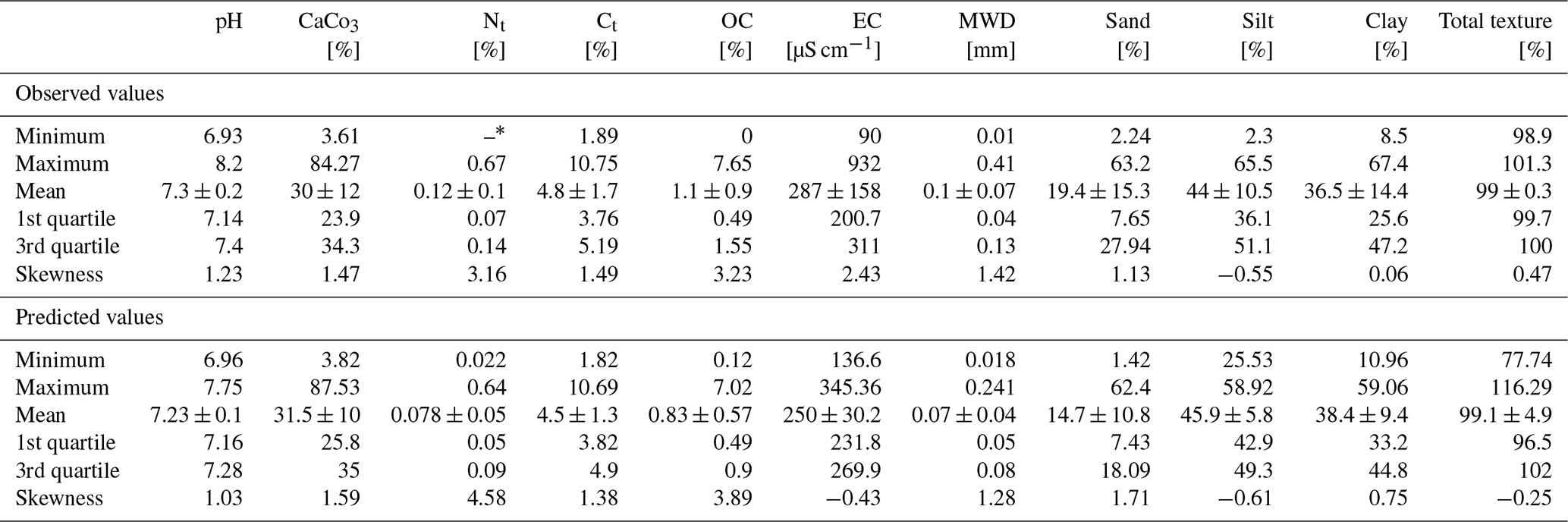
^* Device could not measure concentration below 0.03.

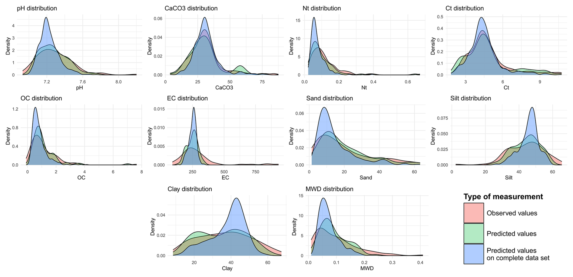
Figure 7 Density plot of the laboratory measurements, the predicted values, from the Cubist model, for the laboratory samples and the predictions of all samples. Realised with R 4.4.0.

3.2 Soil properties spectra prediction

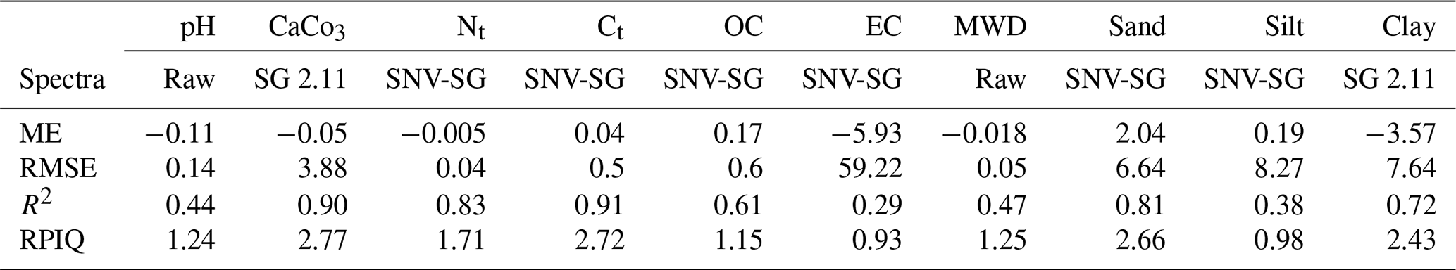
The SNV-SG transformed spectra provided the best performance for six out of the ten soil properties, while SG-SNV and raw spectra were optimal for two properties each (Table 4). Model performance varied substantially depending on the soil property. For pH, predictions showed a slight underestimation bias (ME = −0.11) and a moderate prediction error (RMSE = 0.14). The moderate R² (0.44) indicates a limited ability to reproduce the observed variability. Predicted values displayed a narrower range than the observations and tended to concentrate around the mean (Fig. 7). In contrast, CaCO₃, N_t, and C_t were predicted with higher accuracy. These properties showed minimal bias and relatively small prediction errors (RMSE = 3.88 %, 0.04 %, and 0.5 %). Their high R² values (0.90, 0.83, and 0.91, respectively) indicate that a large proportion of the observed variability was captured by the models. For CaCO₃ in particular, the low bias is notable given the wide range of observed values (Table 3), and the predicted distributions closely matched the observed ones (Fig. 7). The interpretation of N_t remains more cautious due to the strong skewness of its observed distribution. Organic carbon predictions showed a slight overestimation bias (ME = 0.17) and moderate error (RMSE = 0.6 %). Given the high skewness of the observed values, this performance can be considered acceptable, although the R² (0.61) indicates that part of the variability remains unexplained. Regarding the electrical conductivity, the strong underestimation bias (ME = −5.93 µS cm⁻¹), large RMSE (59.22 µS cm⁻¹), and low R² (0.29) indicate weak predictive performance. This suggests that EC is not well captured by the spectral information. The high variability and skewness of the observed EC values likely contributed to this difficulty. Predicted EC values were strongly concentrated in the lower range compared to the observations, as reflected by their smaller standard deviation and distribution pattern (Fig. 7). For MWD, predictions showed a slight underestimation bias and moderate error (ME = −0.018 mm, RMSE = 0.05 mm). However, the model failed to reproduce the upper range of observed values (Table 3). The predicted distribution showed reduced variability, with high MWD values systematically underrepresented. This indicates limited ability of the model to capture extreme aggregate stability conditions. Regarding soil texture, clay content was generally underestimated (ME = −3.57 %), whereas sand and silt showed slight overestimation biases (ME = 2.04 %, 0.19 %). Prediction errors were similar for all three fractions, but a good explanatory power was obtained for sand and clay (R² = 0.81 and 0.72), whereas silt showed weaker performance (R² = 0.38). The silt model particularly failed to represent the lower and higher ends of the distribution, resulting in a concentration of predicted values near the mean (Fig. 7). Overall, predicted texture fractions exhibited lower variability than the laboratory measurements, especially for silt.

Table 4 Cubist model evaluation metrics.

Although the general patterns observed in laboratory measurements were also reflected in the predictions (Table 3), some differences remained. Predicted soil textures were predominantly classified as silty-clay and silty-clay-loam (Fig. 8), with slightly lower clay and higher sand contents compared to observations. The silt and clay classes were proportionally less represented in the predictions than in the observed values.

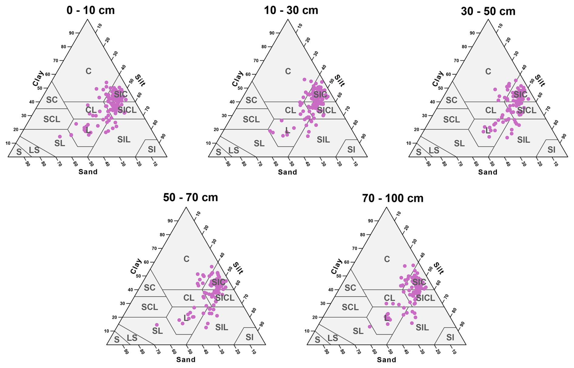
Figure 8 Particle size soil predictions, representation in a triangle diagram, according to USDA classification system (IUSS Working Group WRB, 2022), for each depth increments. C: clay; SC: sandy clay; SCL: sandy clay loam; CL: clay loam; SIC: silty clay; SICL: silty clay loam; L: loam; SIL: silty loam; SI: silt; SL: sandy loam; LS: loamy sand; S: sand. Realised with R 4.4.0.

3.3 Digital soil properties mapping

Feature selection using Boruta substantially reduced the number of covariates by 75 %–93 % (Table 5). Models for deeper soil layers selected fewer covariates than those for the upper layers. The most influential predictors were Landsat 8 SWIR bands and SAVI indices. Sentinel-2 SWIR bands, the EVI index, DEM-derived variables, potential evapotranspiration, wind speed, and solar radiation were also important. Overall, Landsat 8 products performed slightly better than Sentinel-2. These covariates mainly correspond to the s (soil), o (organisms), and r (relief) components of the scorpan framework.

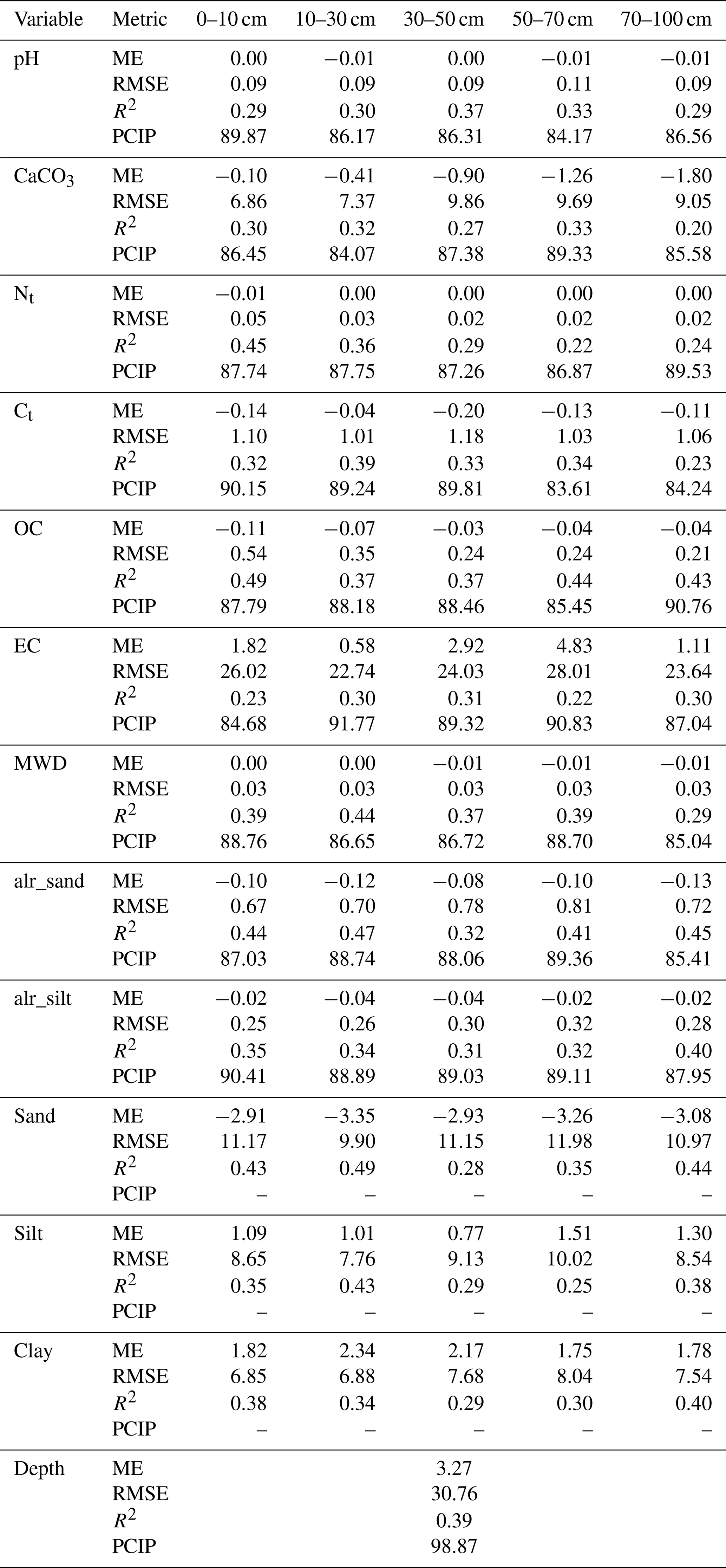
The models generally showed low bias (Table 6), including for EC, where the largest ME (4.83) occurred only in the 50–70 cm layer. Sand and clay were the only variables showing systematic bias, with sand tending to be underestimated and clay overestimated. In contrast to the Cubist predictions, silt performed better than the other texture fractions in terms of bias, although clay had slightly lower RMSE. Overall explanatory power was relatively low, with R² values mostly below 0.5. Some depth-dependent variability in accuracy was observed. For instance, CaCO₃ and clay prediction errors increased with depth, whereas OC showed the opposite pattern, with lower RMSE at greater depths (Table 6). Prediction interval coverage was generally close to the nominal 90 % level, with PICP values mostly ranging between 85 %–95 %, indicating slight overestimation of uncertainty. A few exceptions were observed: pH at 50–70 cm, CaCO₃ at 10–30 cm, and C_t at 50–70 cm. Overall, this suggests that the models were reasonably well calibrated. PICP was not reported for texture fractions. Because log-ratio transformations are nonlinear, nominal coverage may not be strictly preserved after back-transformation.

The spatial distribution of soil properties reveals a clear contrast between the southern and western areas, Selevani and Zakho plains, Tigris riverbanks, and the northern and eastern zones, Bekhair anticline and Little Khabur Valley (Figs. 9, 10, 11, 12 and 13).

Soil pH remained relatively stable with depth and tended to be higher in the anticline and valley areas, except at 50–70 cm where spatial variability increased (Fig. 12). CaCO₃ showed a generally uniform spatial distribution, with localized high values along the southern anticline foothills. N_t concentrations were highest in the topsoil (0–30 cm), particularly in the anticline and north-western areas (Figs. 9, and 10). C_t remained relatively consistent across the upper layers, with maxima near the anticline, while the 70–100 cm layer displayed additional hotspots in the Selevani Plain and appeared strongly influenced by water dynamics (Fig. 13). OC showed depth-dependent spatial shifts, with maxima located in the anticline in the surface layer and in the Little Khabur Valley at intermediate depths. EC was highest in the Selevani and Zakho plains, with secondary peaks in the Little Khabur Valley. Texture patterns indicated higher sand content near the surface and increased silt at 50–70 cm. Sand dominated in anticline and valley areas, whereas silt and clay were more prevalent in the plains. MWD broadly followed texture patterns, with higher values where sand content was greater. Uncertainty maps showed higher values in the Bekhair foothills, Little Khabur Valley, and along the Tigris River (Figs. 9, 10, 11, 12 and 13). For ALR-transformed texture variables, uncertainty values are not directly interpretable due to the nonlinear transformation and should be considered only for relative spatial comparison.

3.4 Soil depth mapping

The soil depth model explained about 39 % of the observed variability, with an RMSE of 30.76 cm. Uncertainty was slightly under-calibrated, as indicated by a PICP of 98.87 % (Table 5). DEM-derived predictors were dominant, with four of the five most influential variables accounting for roughly 25 % of explained variance (Table 6). Spatial predictions revealed two main patterns: shallow soils in mountainous areas and the Little Khabur Valley, and deeper soils in the Selevani and Zakho-Cizre-Silopi plains (Fig. 14).

Table 5 Number of covariates selected with Boruta and top five factors for every soil property.

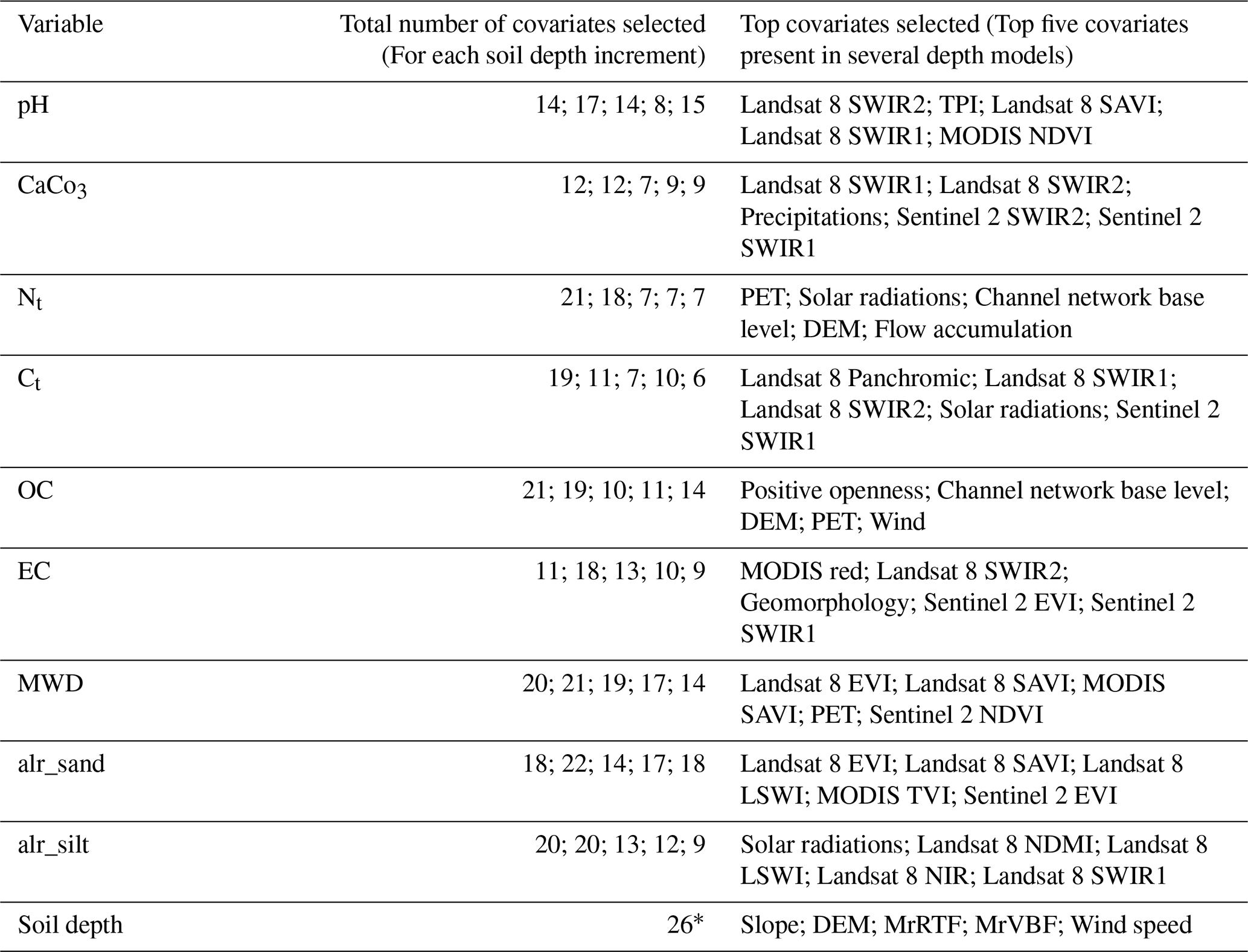
^* No selection of the covariates was performed (see Supplement)

Table 6 Soil properties mapping models evaluation metrics.

4 Discussion

4.1 Spatial interpretations of soil properties distribution

The contrasting distribution of soil properties across the study area (Figs. 9, 10, 11, 12 and 13) can be attributed mostly to landscape differences. The Selevani and Zakho plains, together with the Tigris alluvial valley, largely comprise flat areas along rivers and depressions, which are mainly characterized by sedimentation processes, for example the deposition of flood sediments on river banks and terraces or the filling of depressions with erosion material. In contrast, the little Kabur Valley experiences stronger erosional processes with the formation of rills and gullies, and the Bekhair and Zagros anticlines are subject to uplift at the geological timescale.

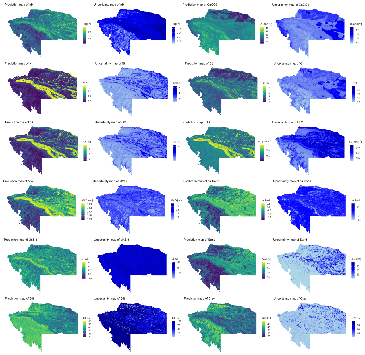
Figure 9 Prediction and uncertainty maps for the 0–10 cm depth increment. Realised with R 4.4.0.

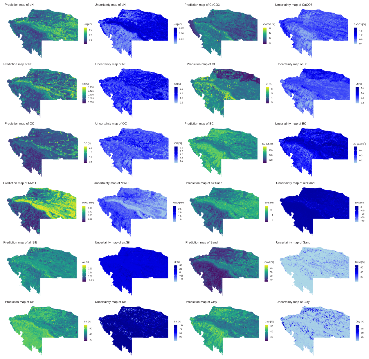
Figure 10 Prediction and uncertainty maps for the 10–30 cm depth increment. Realised with R 4.4.0.

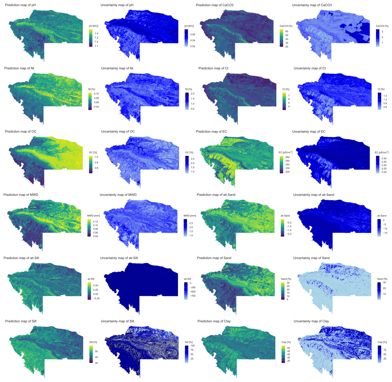
Figure 11 Prediction and uncertainty maps for the 30–50 cm depth increment. Realised with R 4.4.0.

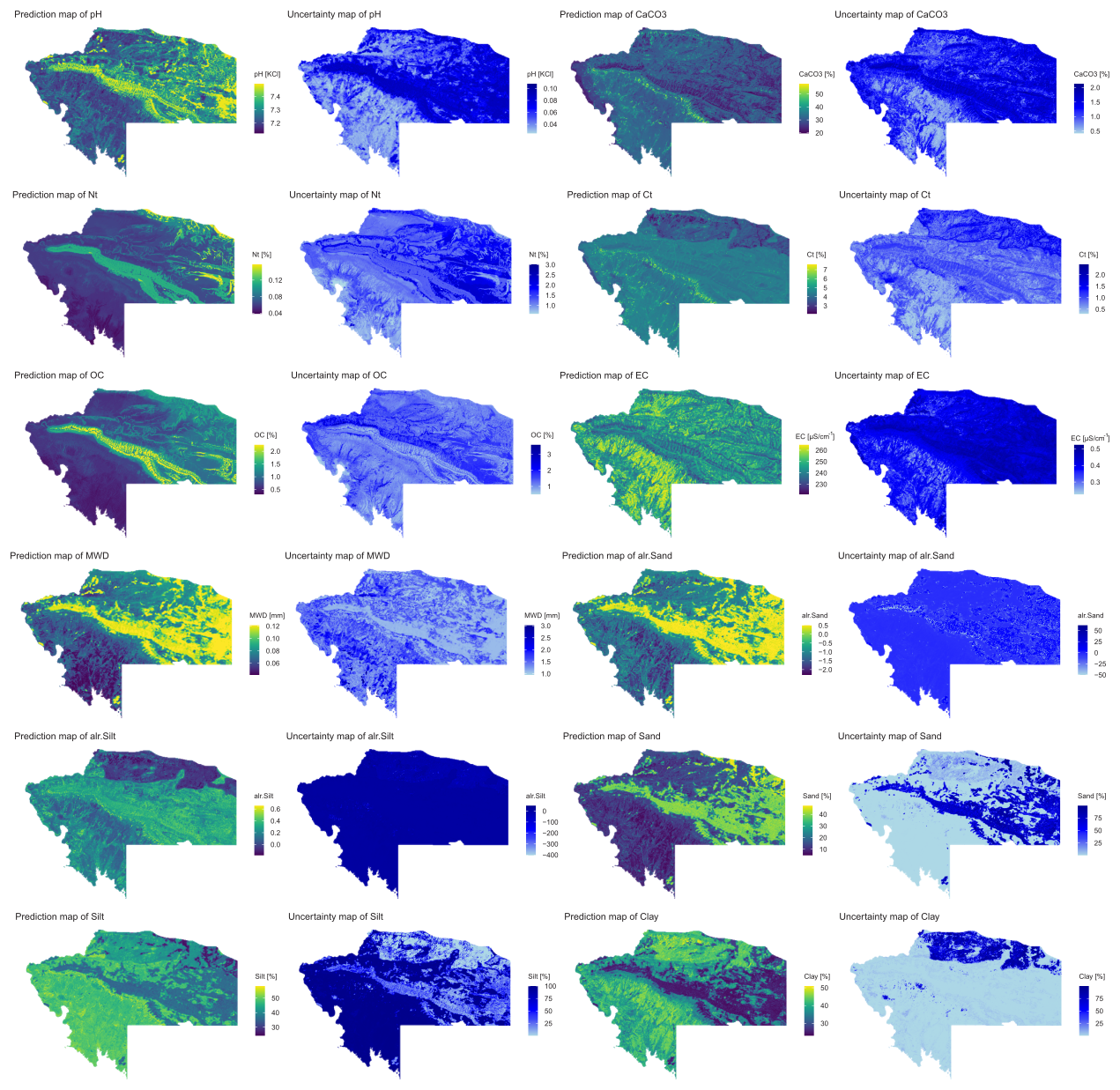
Figure 12 Prediction and uncertainty maps for the 50–70 cm depth increment. Realised with R 4.4.0.

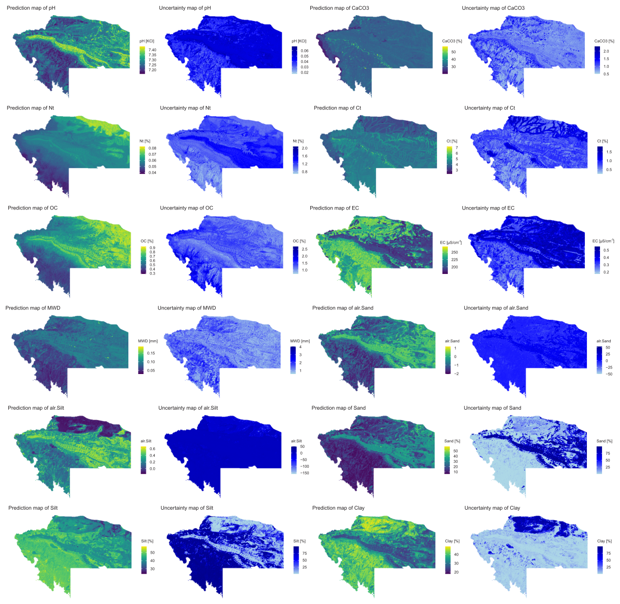
Figure 13 Prediction and uncertainty maps for the 70–100 cm depth increment. Realised with R 4.4.0.

The spatial correlation between pH and EC is particularly evident. Neutral pH values and elevated EC are mainly associated with Kastanozems in the Zakho Plain and calcareous Calcisols or Vertisols in the Selevani Plain. Organic carbon and N_t concentrations are higher in the Little Khabur Valley and mountainous areas, likely linked to denser vegetation cover (Quercus brantii, Quercus boissieri; Zohary, 1973, pp. 183–190) and a cooler climate regime. CaCO₃ content appears to reflect the lithological composition of the Selevani Plain, particularly the carbonate-rich sandstone Injana Formation. Consequently, total carbon (C_t), closely follows CaCO₃ distribution, with the majority of carbon storage deriving from inorganic forms in deeper horizons (Moharana et al., 2021). Textural patterns reveal finer soil fractions (clay and silt) prevailing in the flat plains and the southern foothills of the Bekhair anticline. In contrast, coarse-textured soils with higher sand content are found in more eroded and badlands areas, such as the top of the anticline and the Little Khabur Valley.

Concerning the uncertainty of the predictions, higher values were observed in the Bekhair anticline and Little Khabur Valley, which are areas with greater geomorphological variability and microrelief. This is consistent with the fact that the terrain predictors derived from DEM, may not fully capture the complex topography of these areas. Additionally, the presence of active $w\stackrel{\mathrm{‾}}{a}d\stackrel{\mathrm{‾}}{\mathit{ı}}s$ channels and badlands in these regions may contribute to increased spatial heterogeneity, further challenging the model's predictive performance.

4.2 Soil depth distribution

Two distinct patterns emerged in the spatial distribution of soil depth (Fig. 14). Shallow soils are prevalent in foothill and mountainous regions, as expected (Patton et al., 2018), but are also common in badlands and along active $w\stackrel{\mathrm{‾}}{a}d\stackrel{\mathrm{‾}}{\mathit{ı}}s$ channels, and riverbanks of the Tigris and Little Khabur.

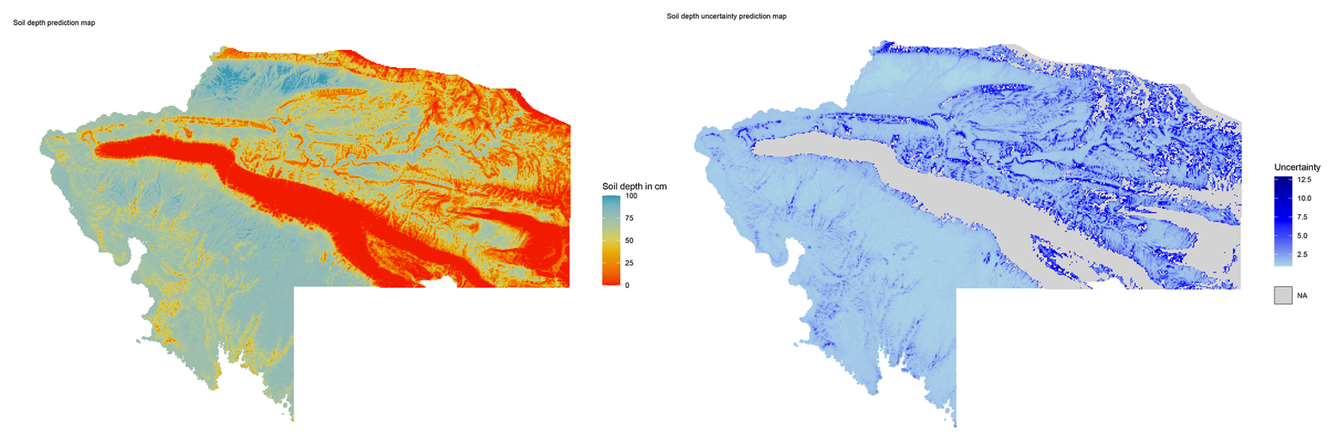
Figure 14 Left: Soil depth prediction map. Right: Soil depth prediction uncertainty map. Realised with R 4.4.0.

In contrast, deeper soils were mapped in the Zakho Plain and on the plateaus of the Little Khabur Valley. These patterns may be explained by flat topography, active depositional process, and in the case of the plateaus, by denser vegetation zones typical of the Kurdo-Zagrosian climate formation.

The soil depth uncertainty map confirms the model’s robustness in predicting both shallow and deep profiles. The highest uncertainty was found near major $w\stackrel{\mathrm{‾}}{a}d\stackrel{\mathrm{‾}}{\mathit{ı}}s$, badlands, and along the foothills – areas with greater geomorphological variability and microrelief. The top-ranked covariates, mainly derived from DEM, confirm the well-established relationship between topography and soil depth (Patton et al., 2018; Yan et al., 2018; Liu et al., 2022).

4.3 SoilGrids 2.0 product comparison

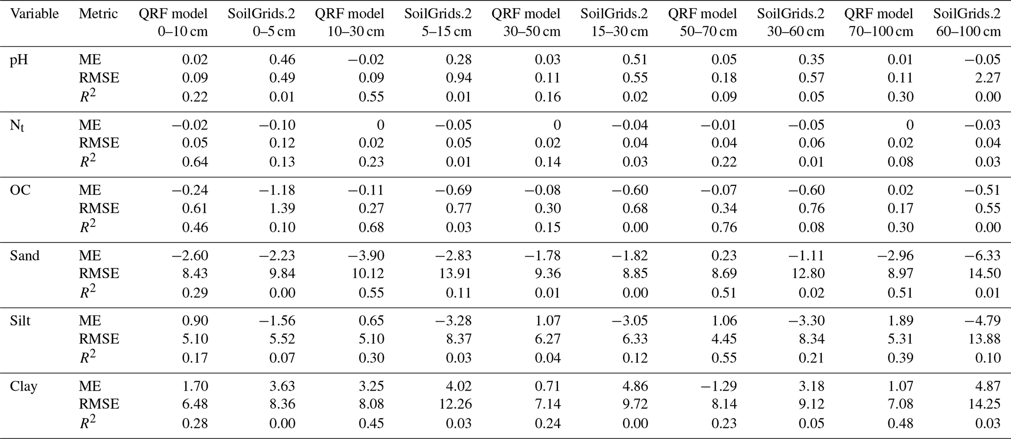
To assess model performance, we compared our results with the global SoilGrids 2.0 product (Poggio et al., 2021), focusing on pH, OC, N_t, and texture attributes (Table 7), for three generalised depth intervals (0–30, 30–60/70, and 60/70–100 cm). We scaled our predictions to match the 250 × 250 m resolution of SoilGrids 2.0, with a bilinear method from the terra package (Hijmans et al., 2025).

Table 7 Comparative statistics of prediction maps with SoilGrids 2.0 model.

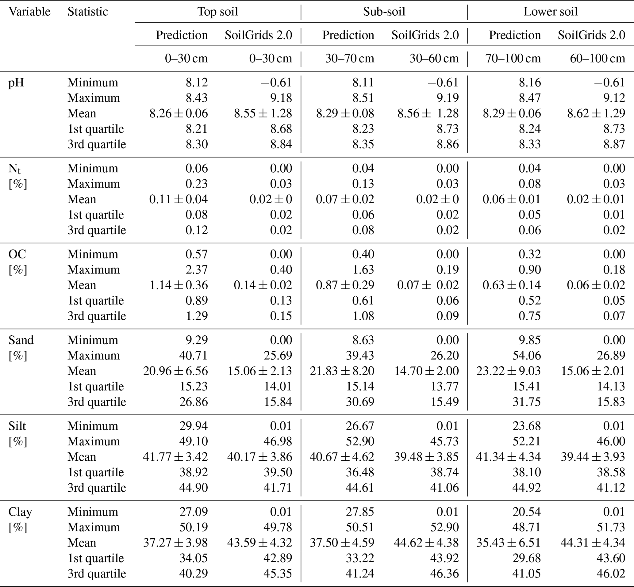
Our models predicted higher values of OC and N_t, with respective increases of ≈ 1000 % and 300 % over those from SoilGrids 2.0. Predicted sand values were also higher (by ≈ 25 %), while clay values were slightly lower (by ≈ 15 %). The differences in silt and pH values were negligible, with a 3 % higher value for silt and 5 % lower for pH in our predictions compared to SoilGrids 2.0.

The standard deviation of the SoilGrids 2.0 product is smaller, except for the pH, than for our prediction models (Table 7). This shows a narrower distribution of values, likely due to the wide range of input data used for the SoilGrids 2.0. The diversity of soil types and input data at the global scale makes the SoilGrids 2.0 model respond relatively homogeneously at the regional scale. Furthermore, the SoilGrids 2.0 product shows a more skewed distribution for OC and N_t, with a higher concentration of values near the lower end of the distribution, which is consistent with the known underestimation of these properties in global models (Shi et al., 2025).

We also compared the evaluation metrics of our predicted values with those obtained from SoilGrids 2.0 on an independant data set (Table F1). Before training the models on a full data set, we splited the data retaining 20 % for test and 80 % for training. The models were trained in similar conditions as our main prediction models (cf. Sect. 2.4.2), before evaluation were computed on the independant test set. Overall, our models outperformed SoilGrids 2.0 across all evaluation metrics for pH, N_t, OC, sand, silt, and clay at all depth intervals. The only exception was the sand QRF model RMSE score at the 10–30 cm depth interval, which was slightly higher for the SoilGrids 2.0 model at the 15–30 cm interval.

Bivariate comparison maps (Fig. 15) indicate that our model yields higher values of pH, N_t, OC, and sand in the Selevani Plain, while SoilGrids 2.0 shows higher values for the same properties in the Little Khabur Valley and the Bekhair anticline. The spatial patterns of silt and clay are inversely distributed. Areas of similarity between the models include pH in the eastern part of the Selevani Plain and Zakho area, OC in the Selevani Plain sporadicly and eastern part of the Zakho Plain. Sand values are similar in the southern foothills of the Bekhair anticline while clay present similarity in the eastern part of the Little Khabur Valley. Due to the use of different algorithms for each depth increment, a direct ensemble model comparison with SoilGrids 2.0 (Varón-Ramírez et al., 2022) was not feasible.

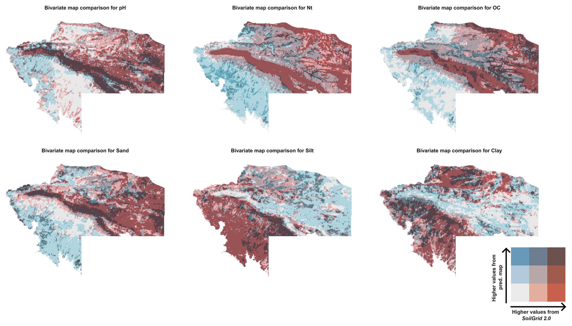
Figure 15 Bivariate map of pH, N_t, OC, and texture from prediction maps vs. SoilGrids 2.0. Realised with R 4.4.0.

4.4 Data quality, limitations, and future applications

The laboratory-measured soil properties and their corresponding FTIR spectra constitute a valuable and reusable dataset that can contribute to improving predictive model performance over time (Viscarra Rossel et al., 2016; Safanelli et al., 2025). Assigning reliability categories to FTIR-based predictions is a common practice to help users interpret results (Wadoux et al., 2021a), and frameworks such as those proposed by Ng et al. (2022b) have supported this effort. However, such categories are not absolute and can vary depending on the study context, input data quality, and intended application. Therefore, although these categories (A–D) provide a useful reference framework, they were not formally applied in this study. Considering the results for the ten predicted properties (Table 4), CaCO₃, C_t, sand, and clay showed comparatively strong predictive performance, with low errors and good explanatory power, suggesting that these models may be transferable to similar contexts. In contrast, pH, N_t, OC, and MWD showed more moderate performances. For OC, this likely reflects the high variability and skewness of the observations, whereas for pH, N_t, and MWD it may indicate weaker relationships with spectral information. EC and silt predictions presented distinct challenges, consistent with known limitations of FTIR-based prediction (Hobley and Prater, 2019; Ng et al., 2022b). In addition, for the EC, the high variability and skewness of the measured values likely limited the model’s ability to capture consistent patterns. Concerning the silt, lower performance may relate to the indirect nature of its spectral response, which is typically more difficult to detect than clay or sand (Janik et al., 2016; Lacerda et al., 2016). Additionally, for the silt, we used MIR spectra and Cubist model, while previous studies have reported improved performance when using vis-NIR data or alternative algorithms such as RF (Hobley and Prater, 2019).

The updated soil classification map (Fig. 6) must be interpreted with care, especially for local agricultural or construction planning. First, arround 90 % of field observations were based on auger sampling rather than full-profile descriptions. Second, the 100 cm depth limit may omit deep horizons, although other local profile observations (Abdulrahman et al., 2020) tend to show that profiles below 100 cm are uncommon. Third, the Tigris right bank was mapped using remote sensing only, which may introduce higher uncertainty. But despite these limitations, the current product offers improved detail over earlier maps (Buringh, 1957; Altaie, 1968), and adheres to modern WRB standards (IUSS Working Group WRB, 2022).

Direct comparison of our model’s accuracy with global datasets such as SoilGrids 2.0 is inherently difficult due to differences in spatial resolution and input data. While SoilGrids 2.0 aims to provide consistent global coverage, our maps, with a resolution of 30 m, offer substantial improvements for regional applications. Notably, the density of training samples used in our study (53.5 per 1000 km²) greatly exceeds that of the WoSIS dataset used for SoilGrids 2.0, which reports a density of only 0.032 per 1000 km² and includes no samples from the Kurdistan Region (Batjes et al., 2020). Furthermore, the use of a conditioned Latin hypercube sampling strategy further enhances spatial representativeness compared to legacy sampling methods (Brus, 2019; Ma et al., 2020).

One limitation lies in the harmonisation of our soil depth intervals with other models (Arrouays et al., 2014; Poggio et al., 2021; Varón-Ramírez et al., 2022; Shi et al., 2025). A second limitation concerns our limited depth observation window of 100 cm, whereas global products such as SoilGrids 2.0 and the Chinese Soil Atlas extend to 200 cm (Shi et al., 2025).

Finally, compared to the prediction model by Yousif et al. (2023), our RMSE values for sand and silt (at 0–10 cm depth) are comparable, while slightly higher than theirs (sand = 9.14; silt = 7.18). However, their clay predictions are more accurate (RMSE = 3.70), and overall model R² is higher (sand = 0.91; silt = 0.85; clay = 0.90). Yet, their model is limited to topsoil (0–30 cm) and focuses only on “soil” areas (202 km²), based on the land use/cover classification (LU/C), while our model covers a broader range of landscapes.

5 Data and repository organisation

The Supplement of this paper contain all additional information and original product divided into eight folders:

1. RUSLE part contains all factor of the RUSLE model map and the map itself.

2. The cLHS part includes the R code and the soil profile points produced for 2022 and 2023 campaigns.

3. The field part contains all the photographs of sampling sites and the raw observations made during the campaigns, including the soil classification map in .gpkc format.

4. FITR element includes all the raw spectra in the .dpt format and the R code used to compile and filter these spectra.

5. Laboratory folder has only one item, the .csv of all the laboratory measurements detailed.

6. The spectra prediction folder includes the Python codes used to predict the soil properties based on the FTIR spectra with a Cubist model, and the predictions results and metrics.

7. DSM folder contains all the codes and exportations from the digital soil mapping made under R including the raw prediction and uncertainty maps.

8. The Soil depth folder is similar to the DSM folder, only with soil depth values.

6 Code and data availability

The final maps products are available at https://doi.org/10.6084/m9.figshare.31320958.v2 (Bellat et al., 2026a) in both Network Common Data Form 4 (NetCDF4) and GeoTIFF (GTiff) formats. Profile depth measurements (https://doi.org/10.1594/PANGAEA.973714, Bellat et al., 2024c), laboratory measurement (https://doi.org/10.1594/PANGAEA.973701, Bellat et al., 2024b) and MIR spectra and its predictions (https://doi.org/10.1594/PANGAEA.973700, Bellat et al., 2024a) are also accessible online. All the supplementary files and raw material is available at https://doi.org/10.57754/FDAT.d5h1h-4x027, Bellat et al., 2026b, and the interactive material visible at https://mathias-bellat.github.io/DSM-Kurdistan/ (last access: 26 March 2026). Code is available in the Supplement but also at the GitHub deposit https://github.com/mathias-bellat/DSM-Kurdistan.git (last access: 26 March 2026) (https://doi.org/10.5281/zenodo.19236909, Bellat and Kakhani, 2026). Finally, we developed an online version of the prediction maps of the soil properties, adapted for colourblind persons accessible at https://mathias-bellat.shinyapps.io/Northern-Kurdistan-map/ (last access: 26 March 2026). The sampling design and Cubist predictive model or spectra transformation were computed with: OS = Windows 11, CPU = Intel I7-9750H 2.60 GHz, RAM = 32 GB 2667 MHZ DDR4 (1–2 h process). For the prediction maps models were computed on the Humanum cloud infrastructure: OS = CentOS 8 (arch x86_64), CPU = 2 ⋅ AMD EPYC 7542 32-Core Processor 2.9 MHz(64 cores), RAM = 16 ⋅ 64 GB 3200 MHz DDR4 (1024 GB), GPU = 2 ⋅ Nvidia A100 40G, (6 h process per map, total 24 h).

7 Conclusions

We developed a complete workflow for digital soil mapping at a regional scale in the Dohuk governorate of the Kurdistan Region of Iraq, combining cLHS-driven sampling, MIR-based soil property prediction, and several machine-learning models to produce 50 soil property maps at 30 m resolution, as well as regional soil depth and soil class maps. Compared with SoilGrids 2.0 and earlier local products, our models offer more locally relevant predictions and improved spatial detail, while also covering a broader set of soil properties and depth increments than previous regional studies. The soil class map further aligns with current WRB standards and benefits from greater observational density than earlier exploratory works.

Beyond these technical achievements, the study highlights the importance of integrating local measurements with models tailored to regional environmental gradients. Global products provide consistent baselines, but they cannot fully capture the geomorphological and topographic contrasts that drive soil variability at fine scales. The superior performance of our regional models demonstrates the complementarity between global and local approaches: global datasets remain essential for broad-scale comparisons, whereas locally calibrated workflows are crucial for operational land management, agricultural planning, and resource assessments.

The proposed workflow is fully transferable to other regions of similar size (2000 km²). Areas with comparable environmental conditions – such as western Iran, northern Syria, or parts of the Mediterranean basin – represent suitable candidates for direct methodological transposition. In addition, the time investment required for the entire process, from sampling design to final DSM production, is relatively modest: in our case, approximately one year (235 person-days). The datasets produced in this study also offer broader reusability, for example, as calibration material for MIR/FTIR spectral libraries (Safanelli et al., 2025; Viscarra Rossel et al., 2016) or as part of a regional or global soil profile archive database (Lachmuth et al., 2025).

A further contribution of this work is the provision of the first regional FAIR-compliant soil dataset (Crystal-Ornelas et al., 2022). Soil science research remains highly geographically imbalanced, with five countries producing more than 80 % of global output (Cherubin et al., 2025). Southwestern Asia is sparsely represented, except for Iran, and no soil profiles from the Kurdistan Region of Iraq appear in the WoSIS database (Batjes et al., 2020) used by SoilGrids 2.0 (Poggio et al., 2021). Such data gaps reinforce global inequalities in environmental knowledge (Allik et al., 2020; Sonnenwald, 2007) and limit the capacity of data-poor regions to benefit from international modelling initiatives. By openly sharing our dataset and workflow, we help reduce this imbalance and contribute to greater transparency and reproducibility in regional soil information systems.

Overall, this project demonstrates that, locally informed digital soil mapping is feasible and highly effective in data-poor regions. The workflow presented here substantially advances soil knowledge in Dohuk Governorate and provides a generalisable and reproducible model for improving soil information in other regions facing similar environmental and data constraints.

Appendix A: Covariates description and features selection

EROS (2020)EROS (2020)Rouse et al. (1974)McFeeters (1996)EROS (2020)EROS (2020)EROS (2020)EROS (2020)EROS (2020)Huete et al. (1994)Huete (1988)Deering (1975)Gao (1996)Fernández-Buces et al. (2006)Chandrasekar et al. (2010)Khan et al. (2001)Bousbih et al. (2019)Abuelgasim and Ammad (2019)Boettinger et al. (2008)Nield et al. (2007)EROS (2013)EROS (2013)EROS (2013)EROS (2013)Rouse et al. (1974)McFeeters (1996)Hulley and Hook (2018)Hulley and Hook (2018)Hulley and Hook (2018)Hulley and Hook (2018)Huete et al. (1994)Wan et al. (2021)Wan et al. (2021)Didan (2021)Vermote (2021)Vermote (2021)Huete (1988)Deering (1975)Khan et al. (2001)ESA and Airbus (2022)Sissakian et al. (1995); Al-Mousawi et al. (2007)Forti et al. (2021)Zanaga et al. (2021)Zomer and Trabucco, 2022; Zomer et al., 2022Fick and Hijmans (2017)Fick and Hijmans (2017)Fick and Hijmans (2017)Fick and Hijmans (2017)Fick and Hijmans (2017)FAO and IIASA (2023)ESA (2022)ESA (2022)Rouse et al. (1974)McFeeters (1996)ESA (2022)ESA (2022)ESA (2022)ESA (2022)ESA (2022)ESA (2022)ESA (2022)ESA (2022)Huete et al. (1994)Huete (1988)Deering (1975)Bousbih et al. (2019)Gao (1996)Fernández-Buces et al. (2006)Chandrasekar et al. (2010)Khan et al. (2001)Abuelgasim and Ammad (2019)Boettinger et al. (2008)Nield et al. (2007)ESA and Airbus (2022)ESA and Airbus (2022)ESA and Airbus (2022)ESA and Airbus (2022)ESA and Airbus (2022)ESA and Airbus (2022)ESA and Airbus (2022)ESA and Airbus (2022)ESA and Airbus (2022)ESA and Airbus (2022)ESA and Airbus (2022)ESA and Airbus (2022)ESA and Airbus (2022)ESA and Airbus (2022)ESA and Airbus (2022)ESA and Airbus (2022)ESA and Airbus (2022)ESA and Airbus (2022)ESA and Airbus (2022)ESA and Airbus (2022)ESA and Airbus (2022)ESA and Airbus (2022)ESA and Airbus (2022)ESA and Airbus (2022)

Table A1 Covariates used for the different process and modelling (Cont. = Continuous data; Dis. = Discrete data; CLHs =  Conditioned Latin Hypercube sampling; DSM = Digital soil mapping; NDWI = Normalised difference water index; NIR = Near-infrared; NDVI = Normalised difference vegetation index; SWIR = Short wavelength infrared; EVI = Enhanced vegetation index; SAVI = Soil adjusted vegetation index; NDMI = Normalised difference moisture index; CORSI = Combined spectral response index; LST = Land surface temperature; TVI = Transformed vegetation index; LSWI = Land surface water index; DEM = Digital elevation model; MrRTF =  Multiresolution index of the ridge top flatness; MrVBF = Multiresolution index of the valley bottom flatness; TPI = Topographic position index; TWI = Topographic wetness index).

Appendix B: Regional environment

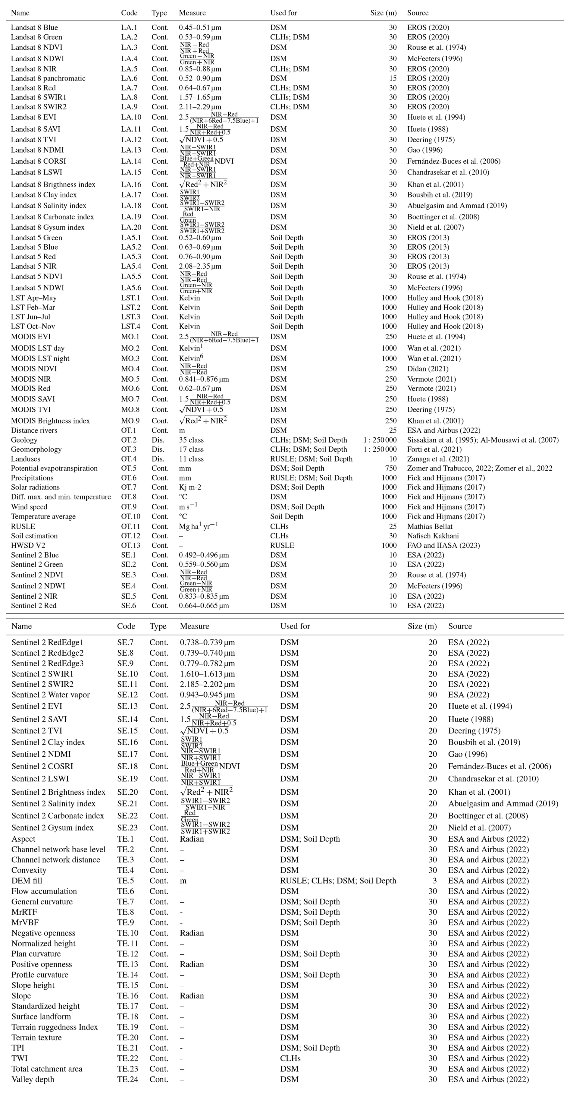
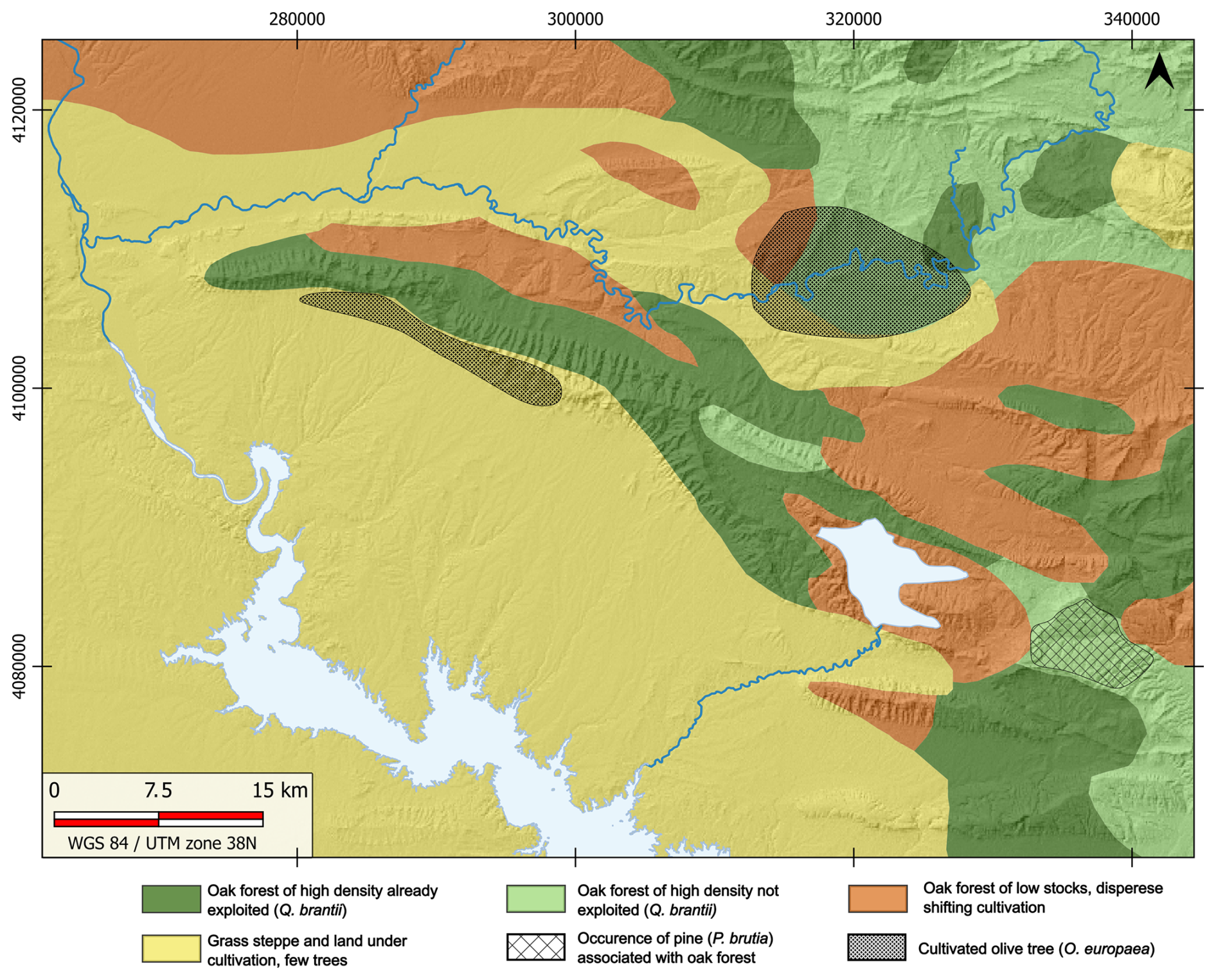
Figure B1 Vegetation map modified from Guest and Al-Rawi (1966). Realised with QGIS 3.34.5 and Inkscape 1.4.

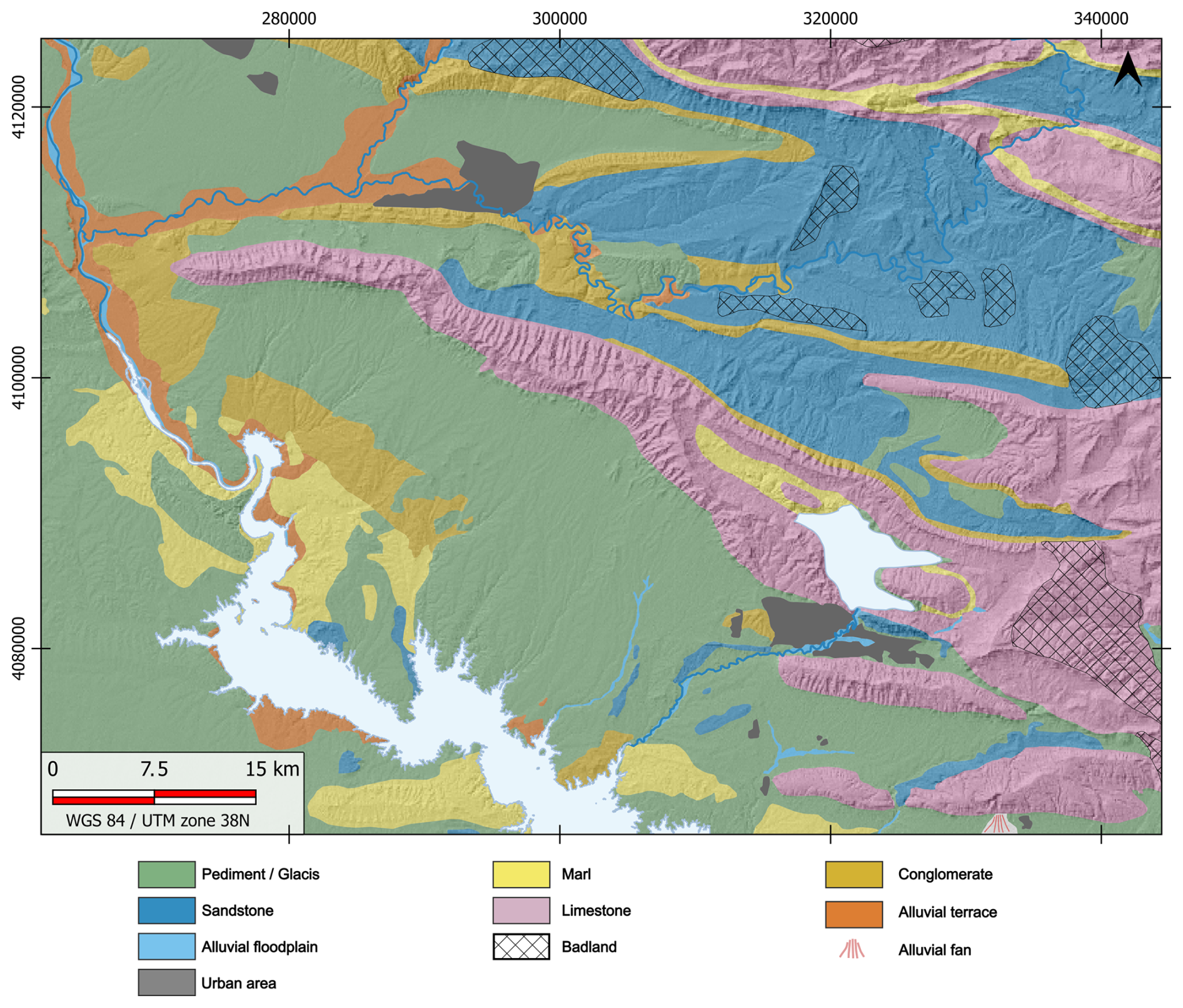
Figure B2 Geomorphological modified map from Forti et al. (2021). Realised with QGIS 3.34.5 and Inkscape 1.4.

Appendix C: RUSLE equations

Table C1 Equations for the performed RUSLE model.

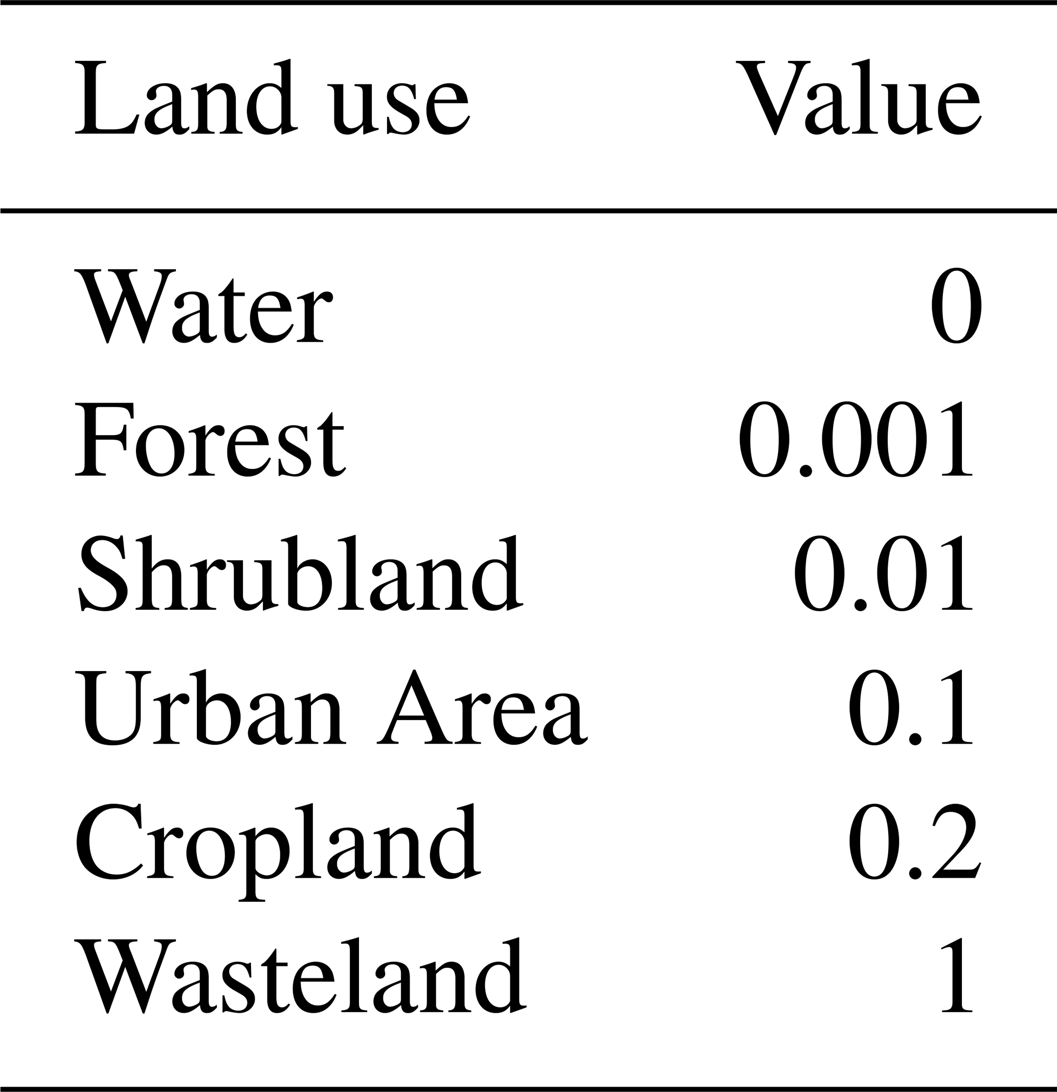
Land use (C) are defined based on (Copernicus, 2019).

$$K=F_{{\mathrm{c}}_{\mathrm{sand}}}\times F_{\text{si-cl}}\times F_{\mathrm{orgc}}\times F_{{\mathrm{hi}}_{\mathrm{sand}}}\times \mathrm{0.1317}$$

where $F_{{\mathrm{c}}_{\mathrm{sand}}}$, F_si-cl, F_orgc and, $F_{{\mathrm{hi}}_{\mathrm{sand}}}$ are defined below.

$$F_{{\mathrm{c}}_{\mathrm{sand}}}=\mathrm{0.2}+\mathrm{0.3}\exp \left(-\mathrm{0.0256}\mathrm{SAN}\left(\mathrm{1}-{\displaystyle \frac{\mathrm{SIL}}{\mathrm{100}}}\right)\right)$$

where SIL is the amount of silt in %.

$$F_{\text{si-cl}}={{\displaystyle \frac{\mathrm{SIL}}{\mathrm{CLA}+\mathrm{SIL}}}}^{\mathrm{0.3}}$$

where SIL and CLA are the amount of silt and clay in %.

$$F_{\mathrm{orgc}}=\mathrm{1}-{\displaystyle \frac{\mathrm{0.25}\mathrm{C}}{\mathrm{C}+\exp \left(\mathrm{3.72}-\mathrm{2.95}\mathrm{C}\right)}}$$

where C is the amount of organic carbon in %.

$$F_{{\mathrm{hi}}_{\mathrm{sand}}}=\mathrm{1}-{\displaystyle \frac{\mathrm{0.7}\left(\frac{\mathrm{SAND}-\mathrm{1}}{\mathrm{100}}\right)}{\left(\frac{\mathrm{SAND}-\mathrm{1}}{\mathrm{100}}\right)+\exp \left(-\mathrm{5.51}+\mathrm{22.9}\left(\frac{\mathrm{SAN}-\mathrm{1}}{\mathrm{100}}\right)\right)}}$$

where SAN is the amount of silt in %.

$${\mathrm{LS}}_j={\displaystyle \frac{S_j\left({\mathit{\lambda }}_j^{m+\mathrm{1}}-\mathit{\lambda }\frac{m+\mathrm{1}}{j-\mathrm{1}}\right)}{\left({\mathit{\lambda }}_j-{\mathit{\lambda }}_{j-\mathrm{1}}\right){\mathrm{22.13}}^m}}$$

where S_j = Slope factor for the jth segment, λ_j= Distance from the lower boundary of the jth segment to the upslope (m) and m= length exponent of the RUSLE Ls factor.

$$R=\mathrm{38.5}+\mathrm{0.35}P$$

where P in the sum of precipitations in one year in mm.

Appendix D: Boruta selections

Figure D1 Boruta feature selection for each soil property. Realised with R 4.4.0.

Appendix E: Tuning hyperparameters for prediction maps

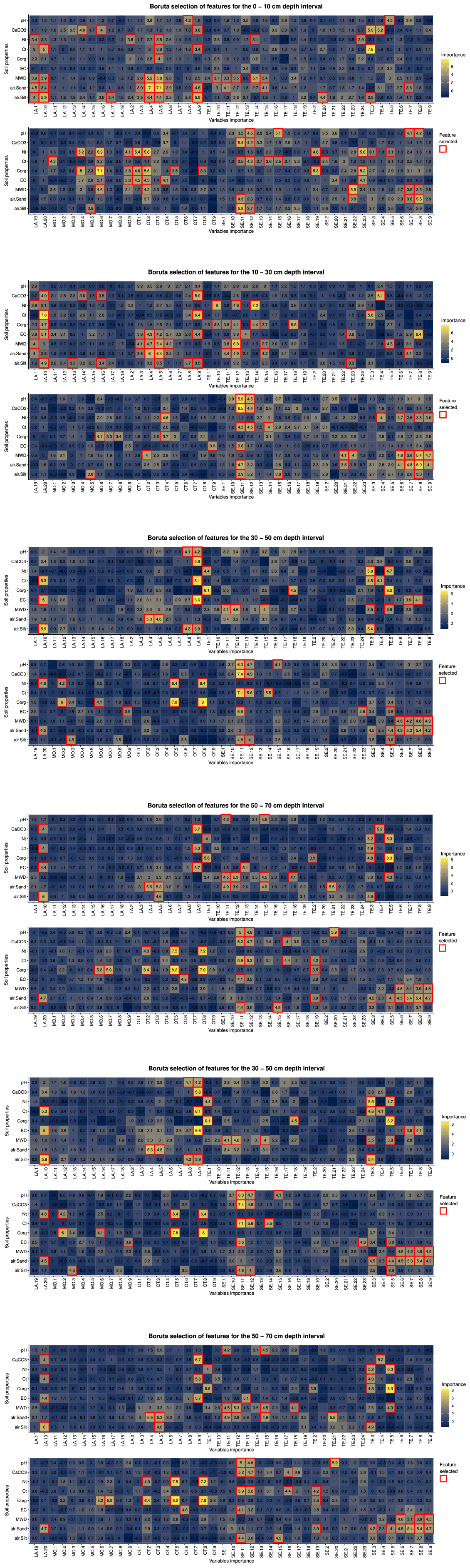
Table E1 Tuning hyperparameters used for the digital soil mapping of soil properties and depth (ntree = Number of trees; mtry = Number of predictors; nodesize = Minimum node size).

Appendix F: SoilGrids.2

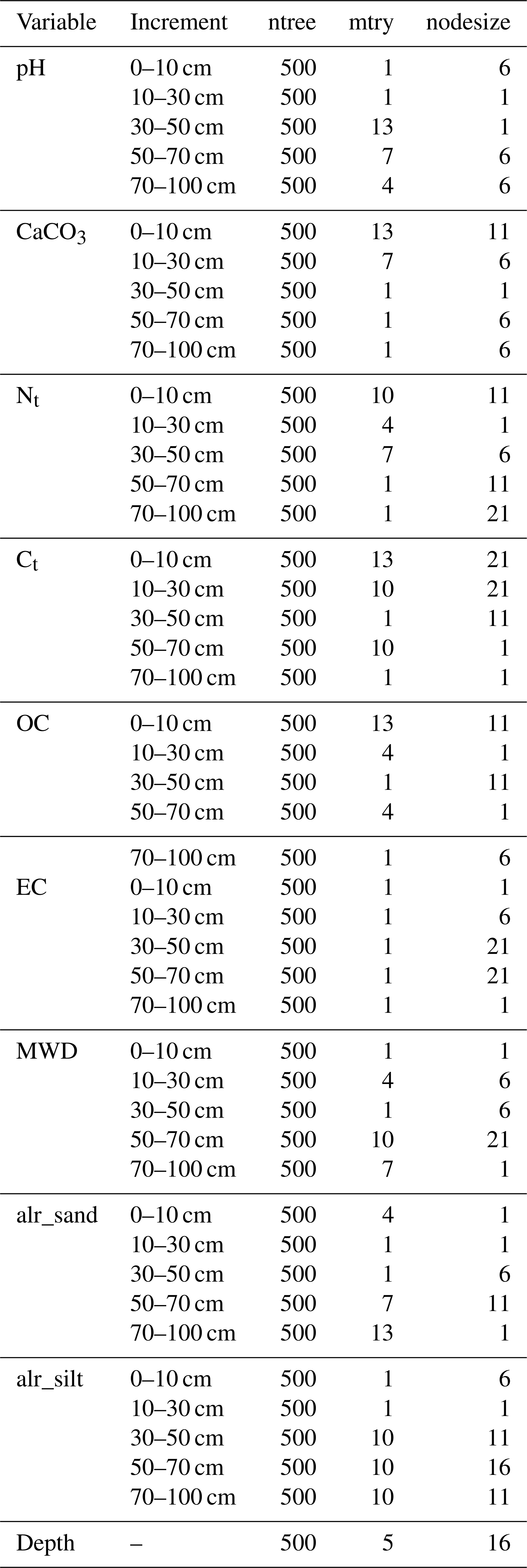
Table F1 Predictions from QRF model vs. SoilGrids.2 model metrics.