Toward better conservation: a spatial analysis of species occurrence data from the Global Biodiversity Information Facility

The world is facing an unprecedented loss of biodiversity, with nearly one million species on the brink of extinction, and the extinction rate accelerating. Conservation efforts are often hindered by insufficient information on crucial ecosystems. To address this issue, our paper leverages advances in machine-based pattern recognition to estimate species occurrence maps using georeferenced data from the Global Biodiversity Information Facility (GBIF). Our algorithms have generated maps for more than 600 000 species, including vertebrates, arthropods, mollusks, other animals, vascular plants, fungi, and other organisms. Validation involved comparing these maps with expert maps for mammals, ants, and vascular plants. We found a close similarity in global distribution patterns, with regional differences attributed to technical variations or necessary revisions in existing expert maps based on GBIF data. As a practical application, we identified the global distributions of approximately 68 000 species with small ranges (25 km × 25 km or less) confined to a single country. Our maps reveal a skewed international distribution of these species, identifying 30 countries where 78.2 % are concentrated. These results highlight the need to integrate the newly mapped GBIF data into global conservation planning. Our algorithms support rapid updates and the creation of new maps as GBIF occurrence reports increase. The data are available on the World Bank Development Data Hub at https://doi.org/10.57966/h21e-vq42 (Dasgupta et al., 2024).

1 Introduction

The world is losing biodiversity at an unprecedented rate. One million plant and animal species may be near extinction, and the pace of extinction is accelerating. According to Pimm et al. (2014), the species extinction rate is at least one thousand times the background rate. The Living Planet Index (https://www.livingplanetindex.org/, last access: 26 January 2026), an indicator of global biodiversity based on population trends for vertebrate species in terrestrial, freshwater, and marine habitats, provides corroborating evidence, showing a 73 % decline since 1970 (WWF, 2024). In response to such alarming indicators, 188 governments in the Convention on Biological Diversity (CBD) ratified the Kunming-Montreal Global Biodiversity Framework (GBF) at the fifteenth meeting of the CBD's Conference of the Parties (COP 15) in December 2022. Among other measures, the GBF committed participants to protecting 30 % of global biodiversity by 2030 (UNEP, 2022). Effectively implementing the GBF requires an understanding of (1) the spatial distribution of global biodiversity to be protected and (2) how protecting 30 % of the planet can best conserve this biodiversity, taking the opportunity value of protected areas into account.

Unfortunately, conservation efforts worldwide are often hindered by limited information on critical ecosystems and biodiversity (Hughes et al., 2024). Comprehensive species coverage is significantly lacking; instead, the predominant focus is on vertebrates and vascular plants, neglecting crucial taxa like invertebrates and other major phyla. This gap creates a policy dilemma for meeting the 2030 GBF commitment of 30 % global protection. If global biodiversity assessments are limited to previously mapped species, policy makers and the conservation community will effectively ignore the enormous population of other species whose occurrences are reported by the Global Biodiversity Information Facility (GBIF). In short, policymakers cannot automatically assume that previously mapped species adequately represent the larger population, a point further discussed by Kass et al. (2022) in the case of invertebrates.

To help bridge the data gap, this study uses GBIF species occurrence records to revisit global biodiversity's spatial distribution. GBIF's reporting network has expanded over 15 years to include over 2 million species' occurrences, with a daily increase of about 1.3 million records in the last two years. Most of these records include locational coordinates, making it possible to estimate the spatial distribution of previously unmapped species, as well as improve estimates for those with existing maps. The algorithm that is presented and implemented in this study generates species maps directly from the GBIF occurrence data, updating the maps automatically as new occurrence data become available. Maps are generated for all species whose data satisfy our computational criteria (currently around 600 000 species). By overlaying the maps with a high-resolution grid, the view of global biodiversity is broadened from the traditional focus on vertebrate animals to encompass greater representation for invertebrates, other animals, plants, fungi, and other non-animal and non-plant species. The maps are then used to develop new indicators of species endemism and identify species with small, vulnerable habitats. Traditionally, species are considered endemic if they reside 100 % in one country; this study examines the effects of lowering this threshold to 95 % and 90 %. Additionally, since small-range status lacks a definitive minimum habitat size, the study explores different area sizes for species with limited occurrence regions.

The study's approach should be viewed as complementary to previous biodiversity assessments (e.g. Map of Life) and can benefit the policy process in several major ways. For existing mapped species, rapid updates using the study's algorithm can help to identify cases where newly reported occurrences suggest alteration of map boundaries. For unmapped species, the approach can provide new information useful for global biodiversity assessments. In addition, the mapping exercise can yield valuable insights on the global distribution of endemic species and small-range species that are especially vulnerable to human encroachment.

The open-access data, algorithm, and programming code developed in this study align with principles of open and equitable sharing of location-specific biodiversity information (Blankespoor et al., 2025; Tanalgo, 2025). It is hoped that this approach would facilitate coordination among countries and enable policymakers, researchers, and conservation practitioners to take informed, coordinated actions to safeguard biodiversity.

2 Data and methods

2.1 Data source and tools

Our data source is an international network funded by the world's governments that provides open access to data about all types of life on Earth. Other international organizations with which the GBIF collaborates include the Catalogue of Life (https://www.catalogueoflife.org/, last access: 26 January 2026) partnership, Biodiversity Information Standards, Consortium for the Barcode of Life (CBOL), Encyclopedia of Life (EOL), and Global Earth Observation System of Systems (GEOSS). The GBIF provides a continuously updated, open-source repository of geolocated, date-stamped reports of species occurrences from many institutions and nongovernmental organizations (NGOs) worldwide. These reports can be accessed directly from the GBIF's Occurrence and Maps application programming interfaces (APIs) at https://www.gbif.org/developer/occurrence (last access: 26 January 2026) and https://www.gbif.org/developer/maps (last access: 26 January 2026), respectively. Its georeferenced data for plants, animals, fungi, and microbes hold the potential for vastly expanding the species domain maps that provide a critical foundation for global conservation planning. Access to the GBIF's full database is offered through Google's BigQuery, Amazon Web Services (AWS), and other cloud-based services.

In this study, we use BigQuery to download the full GBIF database due to its convenient dataset size reduction tools (GBIF, 2024). We limit the GBIF occurrence data to geolocated reports since 1970 for species with at least five unique reporting locations, which our mapping algorithm requires. Since our mapping algorithm operates reliably on several thousand points at most, we cap the data at a maximum of 20 000 randomly selected reports per species to ensure reliability. This limit drastically reduces the size of the download dataset since some species have millions of occurrence records (e.g., the American robin [Turdus migratorius] currently has 21 258 907 reported occurrences). We accept the GBIF's protocols for occurrence report admissibility. Detailed descriptions of the GBIF's protocols and database elements can be found at https://www.gbif.org/data-quality-requirements-occurrences (last access: 26 January 2026).

2.2 Analysis

The premise of our analysis is that species maps underpin spatial analyses of global biodiversity. In theory, if all species are treated equally, a map of global biodiversity could be created by (1) choosing the best available map for each species; (2) overlaying all chosen maps on a high-resolution global grid; and (3) counting the total species incidence in each grid cell. In practice, however, global biodiversity analyses can modify species counting in several major ways. For example, species may be assigned weights, based on the branches they occupy in the “tree of life,” which describes overall genetic variation in the global biome. Also, species weights for conservation priority-setting may vary, based on the species' widely differing vulnerabilities to human encroachment. In addition, the distribution of a species may not be uniform in the spaces enclosed by its maps. If its spatial distribution density is known, its counting weight for each cell can be made proportional to its likelihood of occurrence in that cell. Abundant scientific literature offers examples of weighted species counting (e.g., Guo et al., 2022; Jenkins et al., 2015; Pimm et al., 2014; Veach et al., 2017); however, the requisite research may require detailed genetic and environmental data, as well as expert analysis of their roles in assigning counting weights. Inevitably, the intensive processes involved are time-consuming, requiring technical resources that are in short supply. As a result, a large gap has emerged between the population of species with GBIF occurrence records and that for which research-driven counting weights are available.

The mapping algorithm utilized in this study is a by-product of recent advances in machine-based pattern recognition, cluster analysis, and image processing. In terms of computational geometry, it addresses the problem of efficient bounding of a spatial set, given a subset of actually observed points. Traditional algorithms that draw simple convex hulls poorly represent sets with irregular shapes as a polygon is considered convex if none of its corners bend inward and a convex hull is the smallest convex polygon that encloses all points in a set. In contrast, this study's alphahull algorithm, developed by Pateiro-López and Rodríguez-Casal (2010), which is a function in the R programming language can construct continuous non-convex boundaries for efficient representation. This powerful feature has motivated alphahull's rapid adoption for species range analysis (Guo et al., 2022; Kass et al., 2022).

In our study, alphahull successfully estimates occurrence maps for 92.9 % (567 464) of the 610 694 species in our database. For each of the remaining 7.1 % of species in the database, we employ a standard k-means algorithm to separate occurrence reports into spatial clusters and draw a convex hull around each. We assess the utility of these mapping algorithms for delineating species occurrence regions, with illustrative examples provided in the Annex. Our algorithms estimate occurrence maps for terrestrial, coastal, and marine species.

2.3 Spatial selection bias

We acknowledge that GBIF occurrence reports are often produced by voluntary exercises that do not utilize scientific sampling methods. As a result, spatial point densities in species occurrence reports are positively related to physical accessibility, population density, and income (Borgelt et al., 2022; Garcia-Roselló et al., 2023; Isaac and Pocock, 2015; Reddy and Dávalos, 2003). This means that (all else being equal) species sightings are more likely to occur in areas (1) near transport arteries; (2) with a greater number of inhabitants to identify species, and (3) where more inhabitants have enough disposable income to support species search and reporting costs.

These factors complicate attempts to map species population densities from occurrence reports (e.g., Kass et al., 2022). Our alphahull and clustered convex hull estimators for boundaries differ because they focus on exterior points in spatial sets. Even so, accurate representation requires a critical minimum number of sightings in areas not advantaged by transport access, high population density, or sufficient disposable income. As the occurrence of sightings in non-advantaged areas increases, so does the accuracy of boundary estimation (Feeley and Silman, 2011). Given that the GBIF occurrence inventory is growing by about 1.3 million new reports per day, one can expect that, over time, increased sightings will improve the boundary estimates for sparsely reported species.

3 Results

3.1 Pilot example

To illustrate the results of our mapping algorithm exercise, we take the example of the species Lagidium viscacia (common name: Mountain Viscacha), whose range extends from areas in Argentina and Chile to Bolivia and Peru. In Fig. 1, a comparison of panels a and b shows that the reported sightings of this species include a few points beyond the northern boundary of the expert range map (Burgin et al., 2020a), along with many points beyond the southern boundary. Panel c, which displays the output of our mapping algorithm, shows that the alphahull boundary follows the curvilinear north-south orientation of the point set, widening and narrowing as the point set expands and contracts. As shown, it overlaps heavily with the map of Burgin et al. (2020a), but extends its northern and southern boundary areas to incorporate these sightings.

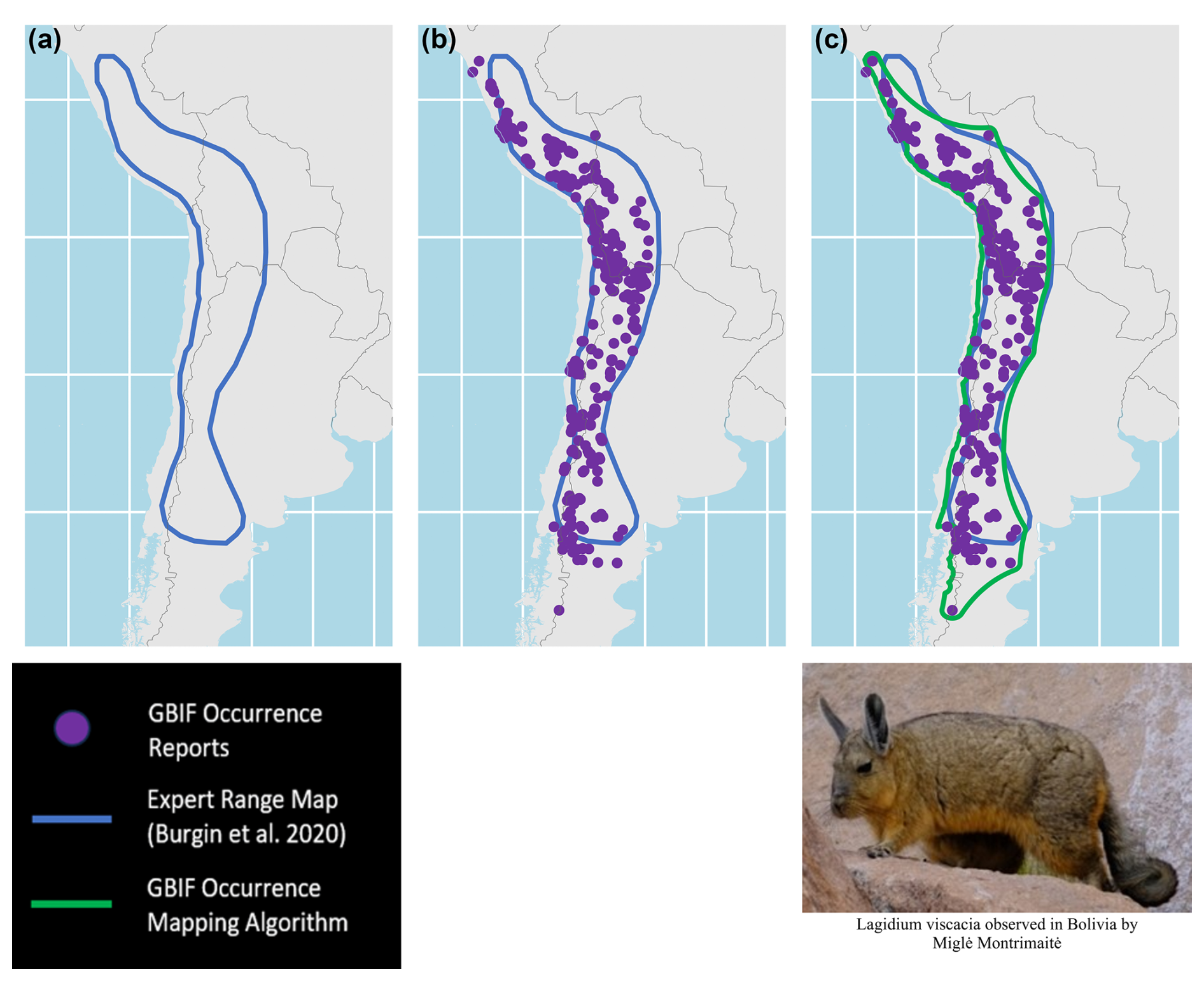
Figure 1 Mapping exercise results for Lagidium viscacia (Mountain Viscacha), showing overlapping boundaries: (a) Expert range mapping boundary in blue from Burgin et al. (2020a), (b) Overlay of GBIF occurrence report locations in purple with the expert range mapping boundary in blue from Burgin et al. (2020a), and (c) Overlay of the GBIF occurrence mapping algorithm in green with GBIF occurrence report locations in purple with the expert range mapping boundary in blue from Burgin et al. (2020a).

3.2 Overall mapping results

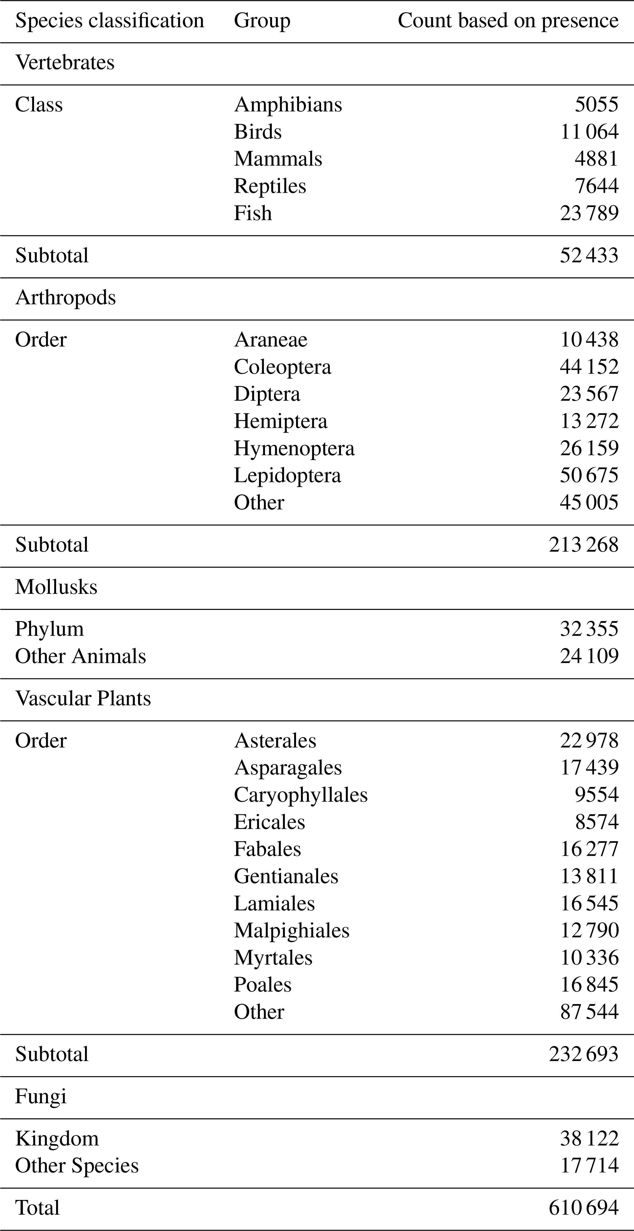
Occurrence record maps were computed for 610 694 GBIF species, comprising 52 433 vertebrates (amphibians, birds, fish, mammals, and reptiles), 213 268 arthropods, 32 355 mollusks, 24 109 other animals, 232 693 plants, 38 122 fungi, and 17 714 other species (the kingdoms Archaea, Bacteria, Chromista, Protozoa, and Viruses) (Table 1).

Table 1 GBIF species occurrence maps.

The exercise was limited to GBIF species in three kingdoms (Animalia, Plantae, and Fungi) with at least three unique geolocated occurrences since 1970. To remove spurious observations from locales (e.g., zoos and botanical gardens), we relied on the following two methods: (1) exclusion of isolated outlier occurrences before map estimation, which happens automatically in our mapping algorithms and (2) exclusion of bounded point sets with fewer than three observations after map estimation. For the many species maps that have multiple bounded areas, we imposed a conservative interpretation of the evidence, dropping species maps with single-bounded areas when they contain fewer than three observations. Although this final condition may seem redundant; it is important to include as a species can pass the initial condition and fail the final one since our estimation algorithms may exclude an outlier point or two from their computations of the bounded areas. Examples of the convex and alpha hull comparisons are included in Appendix A (Sect. 2).

3.3 Case comparisons

To test our species boundary mapping from the current inventory, we ask whether the view of global biodiversity distribution it provides is consistent with that of existing expert maps. On comparing our estimated GBIF occurrence maps with publicly available expert maps from recently published research, we find that thousands of species with GBIF maps have been mapped by the research teams. Using these matched species, each comparison assesses the similarity in global biodiversity patterns produced by our GBIF maps and the expert research products by rank group based on the pixel level distribution of the species maps from 1 (lowest count) to 10 (highest count). Where the patterns diverge, we explore the technical factors that can explain the differences. The first case comparison retains the traditional focus on vertebrates, comparing mammal range maps estimated by Marsh et al. (2022). The second one focuses on a comparison with maps for ants developed by Kass et al. (2022), while the third centers on a limited set of vascular plants mapped by Borgelt et al. (2022). Invertebrates are significantly underrepresented in existing expert maps (Kass et al., 2022). At the outset, it should be noted that this study's major contribution is the expanded coverage of invertebrates. As shown in Table 1, our work offers more comprehensive representation by estimating maps for 213 268 arthropods.

3.3.1 Mammals

Marsh et al. (2022) map the native ranges of mammals globally using the authoritative taxonomy provided by the Mammal Diversity Database (Burgin et al., 2018). Their exercise harmonizes species maps from the Checklist of the Mammals of the World (Burgin et al., 2020b, c; MDD, 2020), and the Handbook of the Mammals of the World published in nine volumes by Mittermeier et al. (2013), Wilson et al. (2016, 2017), and Wilson and Mittermeier (2009, 2011, 2014, 2015, 2018, 2019). In our GBIF occurrence maps database, we identify 3530 mammals that are also mapped by Marsh et al. (2022). We rasterize both sets of maps using a global grid with 0.05° (5 km) resolution. For each species map, rasterization assigns a value of 1 to grid cells that overlap with the map and 0 to other cells. Next, we compute species densities by cellwise addition across 3530 rasters for each set. Figure 2 compares cell counts, which are ranked in 10 groups. The maps' broad patterns are visibly similar. Both assign ranks in the highest two groups to Central America, northwest South America, West Africa, East Africa, the northern region of Central Africa, the eastern region of southern Africa, Western Europe and Southeast Asia. Notably, they also differ in other regions. The GBIF map assigns higher ranks to large areas of Mexico, western United States, and eastern Australia and lower ranks to the southeastern Amazon region and South Asia (also see Fig. A1).

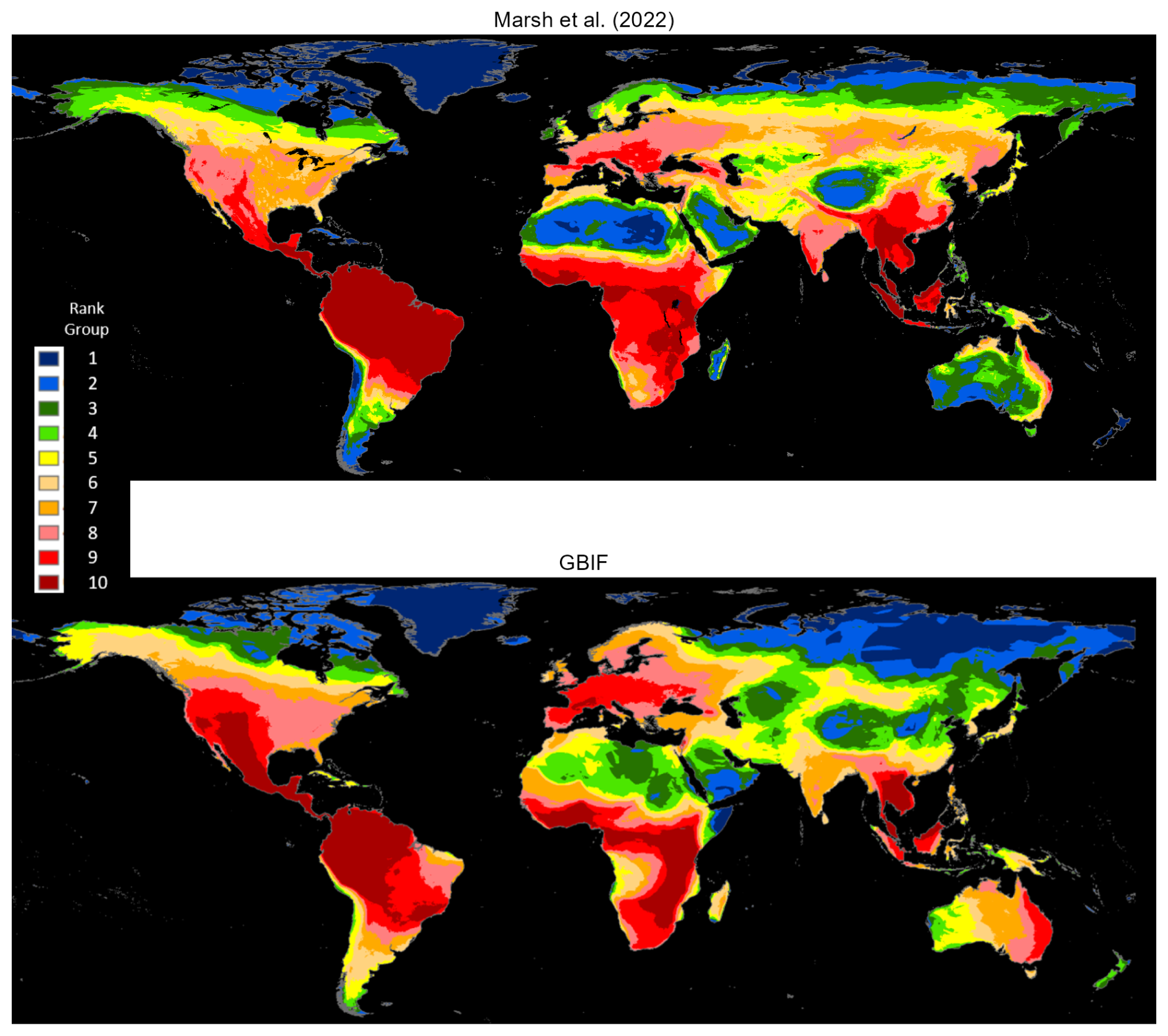
Figure 2 Matched mammals species densities: Marsh et al. (2022) versus GBIF occurrence reports.

Technical differences can explain divergences in the two patterns. For example, the Marsh et al. (2022) maps estimate native ranges of global mammals, taking into account recorded historical occurrences and biogeographical factors that correlate with the range of each mammal species. By contrast, the GBIF mammal maps bound the areas where species occurrences have been reported since 1970. Regions where GBIF ranks are higher than Marsh et al. (2022) ranks have many species with reported occurrences beyond their estimated native ranges; regions with lower GBIF ranks have occurrence reports clustered in subareas within native ranges. This difference could reflect underreporting for GBIF species in lower-ranked areas, although many higher-ranked areas appear similarly disadvantaged for species observation. In our view, the more plausible explanation is that lower-ranked regions are populated by many species whose ranges have contracted over time. The ongoing accumulation of GBIF species occurrence reports should help to resolve this issue.

Figure 2 compares 3530 mammals with maps in both databases, while Fig. 3 does the same for all mapped terrestrial mammals (4138 for GBIF and 6360 for Marsh et al., 2022). Comparison with Fig. 2 reveals almost no difference for GBIF; however, Marsh et al. (2022) have generally higher rankings for Indonesia and Papua New Guinea. Mammal species may be underrepresented in GBIF occurrence reports from the two countries, although this seems more likely for sparsely populated Papua New Guinea than densely populated Indonesia (also see Fig. A2). The more likely explanation, in our view, is that the areas populated by many mammals have contracted.

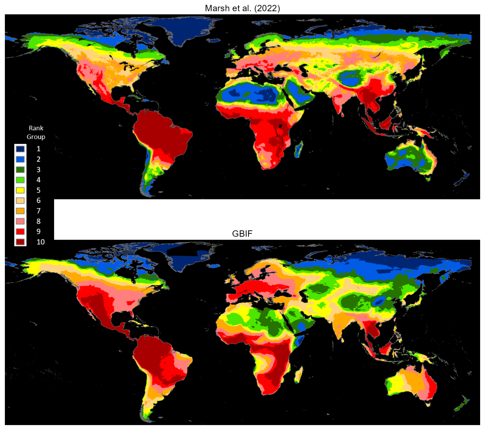
Figure 3 Full mammal species densities: Marsh et al. (2022) versus GBIF occurrence reports.

3.3.2 Ants

Clark and May (2002) identified a severe taxonomic bias in conservation research, finding that vertebrates accounted for only 3 % of described species but 69 % of published papers. Conversely, invertebrates accounted for 79 % of described species and just 11 % of published papers (Leather et al., 2008). Kass et al. (2022) address this problem for ants using a variety of datasets and techniques, including the alphahull algorithm, to estimate the range maps. In our GBIF occurrence maps database, we identify 5445 ant species also mapped by Kass et al. (2022). We rasterize both sets of maps using a global grid with 0.05° (5 km) resolution and compute species densities by cellwise addition across 5445 rasters for each set.

Figure 4 compares the cell counts, which are ranked in 10 groups. Many areas exhibit similar patterns, including northern North America, Mexico, Central America, northwest South America, Eastern and Western Europe, West Africa, southern Africa, Madagascar, and eastern Australia. However, there are three notable differences. First, both maps identify a large high-ranking region in the Western Hemisphere, which is further north for GBIF than for Kass et al. (2022). Second, both maps identify a band of relatively high ranks across West and northern Central Africa, linking to a north-south band in East and southern Africa; however, the rankings for GBIF are generally lower than those for Kass et al. (2022). Third, Southeast Asia ranks uniformly higher for Kass et al. (2022) than for GBIF (also see Fig. A3).

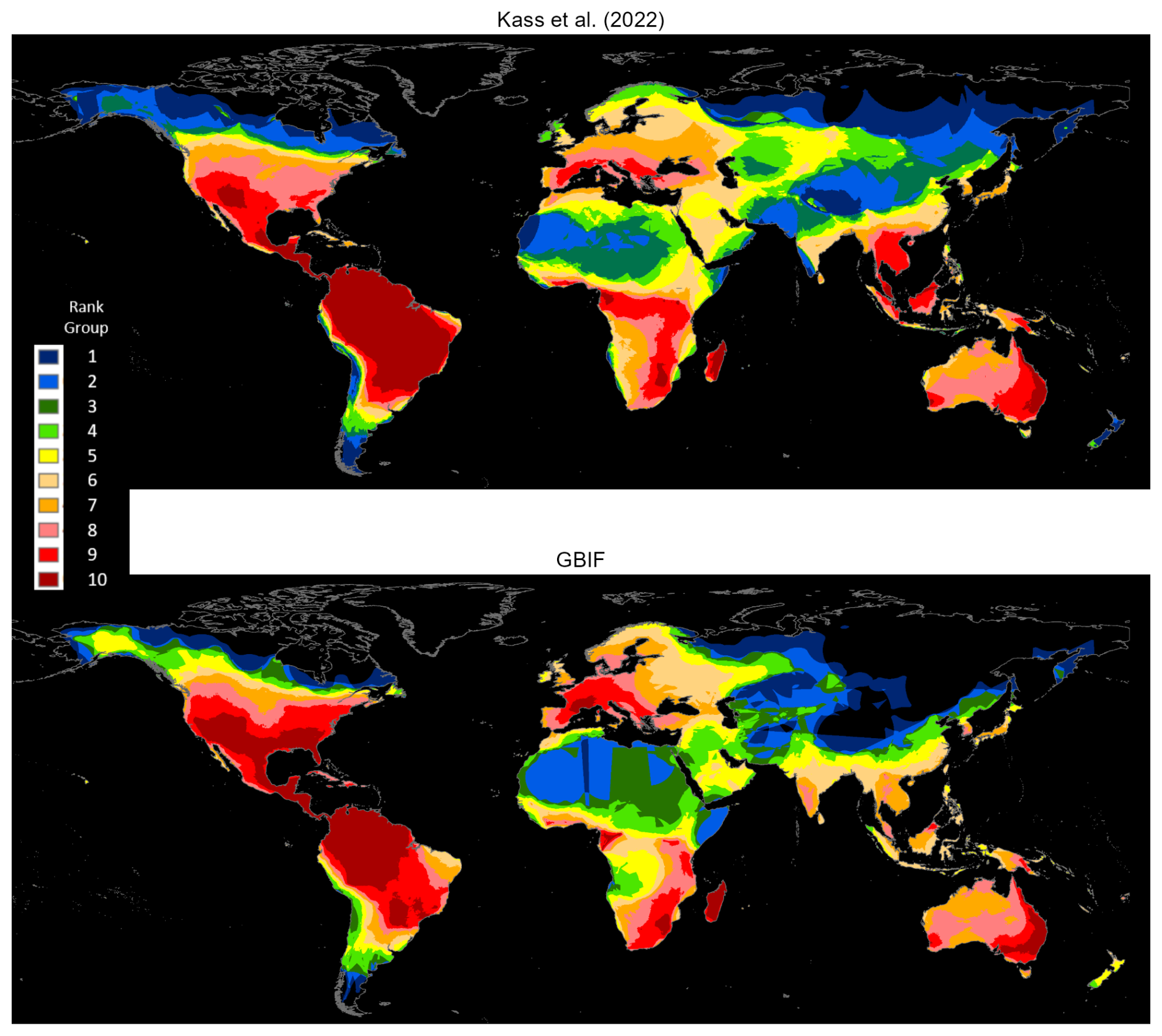
Figure 4 Matched ant species densities: Kass et al. (2022) versus GBIF occurrence reports.

Since Kass et al. (2022) also rely heavily on the alphahull methodology, we attribute these differences to two technical factors. First, their database comes from intensive processing and error checking of records drawn from the Global Ant Biodiversity Informatics (GABI) database in July 2020. In our study, by contrast, the records are drawn from GBIF occurrence data, as of July 2023. Second, our approach is significantly more conservative. For example, we exclude unique species occurrences that number fewer than three, while Kass et al. (2022) include them; since alphahulls cannot be estimated for these 5168 ant species, Kass et al. (2022) estimate their ranges by drawing 30 km buffer zones around the occurrence locations. Given this difference, comparing full database results for GBIF and Kass et al. (2022) would be, in effect, comparing apples and oranges.

3.3.3 Vascular plants

Borgelt et al. (2022) have recently developed spatial density maps for vascular plants in the International Union for Conservation of Nature (IUCN) Red List (IUCN, 2022). They utilize maximum entropy (Maxent) models that predict the likelihood of species occurrences from the values of several environmental variables. For each species, they identify native regions from a web-scraping exercise using the Plants of the World Online (POWO) database, with regional identification standardized from the World Geographical Scheme for Recording Plant Distributions (WGSRPD). Typically, the resulting native regions are the boundaries of small countries or provinces (Database of Global Administrative Areas, GADM, level-1 administrative units) in large countries. Borgelt et al. (2022) estimate the models using GBIF occurrence data with restrictive prior conditions. To preserve compatibility with the environmental variables used for Maxent estimation, the data are confined to the 2000–2020 period. For each species, georeferenced occurrence reports exclude all observations outside pre-identified native regions, and Maxent-estimated species distributions are also confined to native regions. The advantage of this approach is that it guarantees the exclusion of spurious observations from such entities as botanical gardens and private collections in other regions. One drawback, however, is that it incurs the cost of excluding potentially large numbers of occurrence observations that lie outside pre-identified native regions that are arbitrarily defined by national or provincial boundaries.

Unlike Borgelt et al. (2022), our exercise is not constrained by the need for compatibility with environmental modeling variables; therefore, we draw on a longer time period (1970–2023). Also, we impose no prior geographic restrictions on the data. As previously explained, our methodologies estimate occurrence map boundaries after eliminating spurious single outliers and small, isolated occurrence clusters. We identify 32 339 vascular plant species found in both databases, and, as before, rasterize our occurrence maps and compute cell counts at 5 km resolution. As Borgelt et al. (2022) provide species maps in a raster stack with much coarser resolution (50 km), we next extract raster layers for these 32 339 common species and add across layers to obtain relative incidence scores for the 50 km grid cells. Finally, we use mean smoothing to approximate the effect of higher resolution.

Figure 5 displays the comparative results as ranks in 10 groups; the two maps share essentially the same density pattern, except for the somewhat more extensive high-ranking areas in South and Southeast Asia for the Borgelt et al. (2022) maps and the United States for our study's maps (also see Fig. A4).

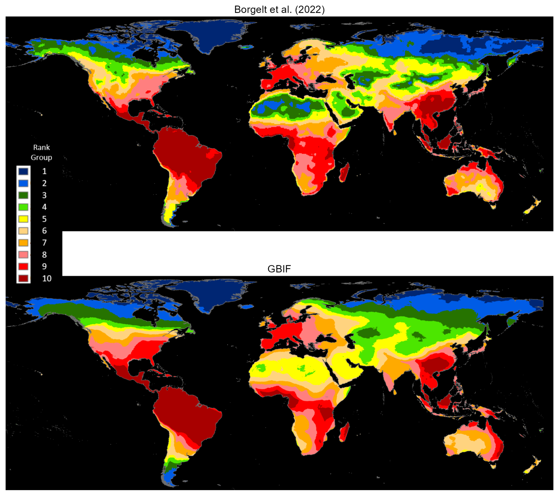
Figure 5 Matched vascular-plant species densities: Borgelt et al. (2022) versus GBIF occurrence reports.

3.4 Summing up

In all three case comparisons, we find quite similar global patterns of species density with strong agreement between the sources for each case. From a confusion matrix of 5 to 10 classes based on distribution of the species rank group, we find that across these taxa overall accuracy and agreement are significantly better than random (accuracy p-value = 0) with plants consistently outperforming ant and mammals (see discussion in Appendix A1, and Table A1). Additionally, we calculated the local Spearman correlation coefficient for each case and found high agreement in areas with low population and levels of lights at night. Where the patterns diverge, the discrepancies can be traced to technical differences. In the case of mammals, differences between the GBIF and expert native-range maps can be attributed to either undershooting, where expert map boundaries exclude many GBIF occurrences, or overshooting, where GBIF occurrences are persistently absent in parts of the native-range maps. In the case of ants, where the research also utilizes alphahull estimation, differences are attributable to differences in source databases and our relatively conservative approach to map estimation. Finally, in the case of vascular plants, where the research employs GBIF occurrences and the global pattern similarity is most striking, the few discrepancies are attributable to temporal and spatial restrictions imposed by the expert research team.

4 Priority-setting applications

The effectiveness of biodiversity conservation plans will require identification of occurrence regions for species with elevated extinction risks. While multiple approaches exist for setting conservation priorities, decisions on resource allocation are typically made at national and subnational levels, particularly in the Low- and Middle-Income Countries. Endemic species and those with very restricted ranges provide a practical entry point, as they are highly vulnerable, confined to smaller geographic areas, and relatively straightforward to target with conservation measures. Protecting these species not only contributes to global biodiversity goals but also safeguards the unique natural heritage of individual nations, creating an added incentive for action. Therefore, using the maps developed with GBIF data, we explored (1) species endemic to a single country and (2) species under continuous threat owing to their small occurrence regions. Our database reflects GBIF-sourced occurrence maps for previously unmapped species, as well as revised estimates for those with existing maps.

4.1 Endemic species distribution by group and country

With the new dataset, we explored the endemic status assigned to species that are 100 % resident in a single country. By this criterion, 44.6 % (272 189) of the 610 694 species maps tabulated by country are classified as endemic. The incidence of endemism differs widely by species group (e.g., 54.5 % for mollusks, 48.7 % for vascular plants, 47 % for other animals, 44 % for arthropods, 37.1 % for vertebrates, and 29.5 % for fungi).

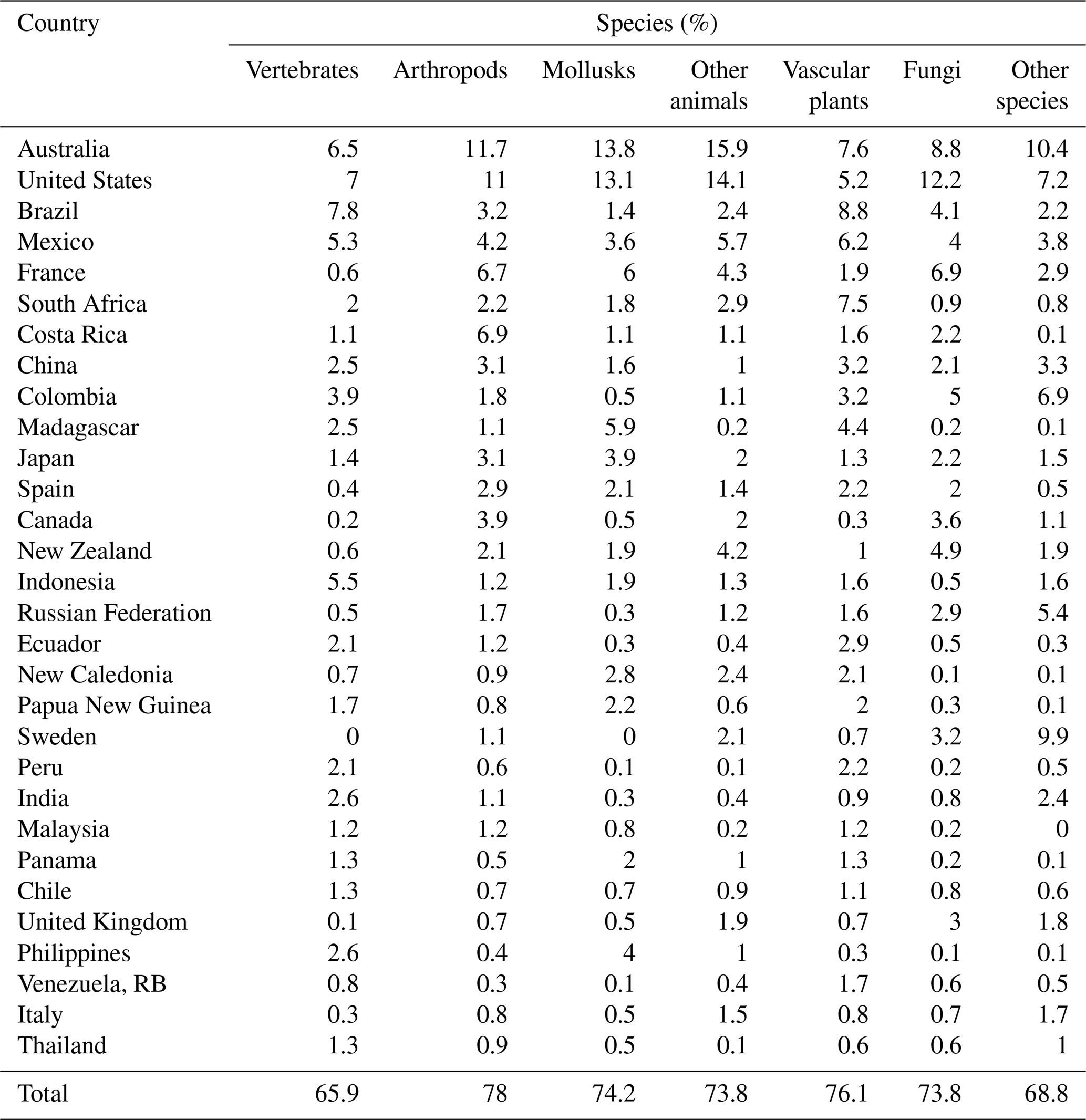
We also count endemic species by country and species group. Country scale plays a major role in raw counts, so we standardize by total country species to highlight the relative importance of endemicity in each country and species group. Table 2 provides a summary for the top 30 countries in each species group, sorted in descending order by average ranking for the seven groups. Overall, the top 30 have 86.6 % (235 706 out of 272 189 species); and our results assign overall top 10 status to Australia, United States, Brazil, Mexico, South Africa, China, New Zealand, Madagascar, Japan, and Costa Rica. Even for the top 30 countries, endemicity varies enormously by species group. In terms of vertebrates, for example, 62 % are endemic in Australia versus only 3 % in the United Kingdom. For plants, the endemicity in Madagascar, Australia, and New Zealand is extremely high, at 89.6 %, 88.1 %, and 84.4 %, respectively. For arthropods, the maximum endemicity is even higher in New Zealand and Australia, at 92.8 % and 91.2 %, respectively. Mollusks, fungi, and other species more closely resemble arthropods and vascular plants in the relative compactness of their ranges.

Table 2 Top 30 countries for species endemism, by group.

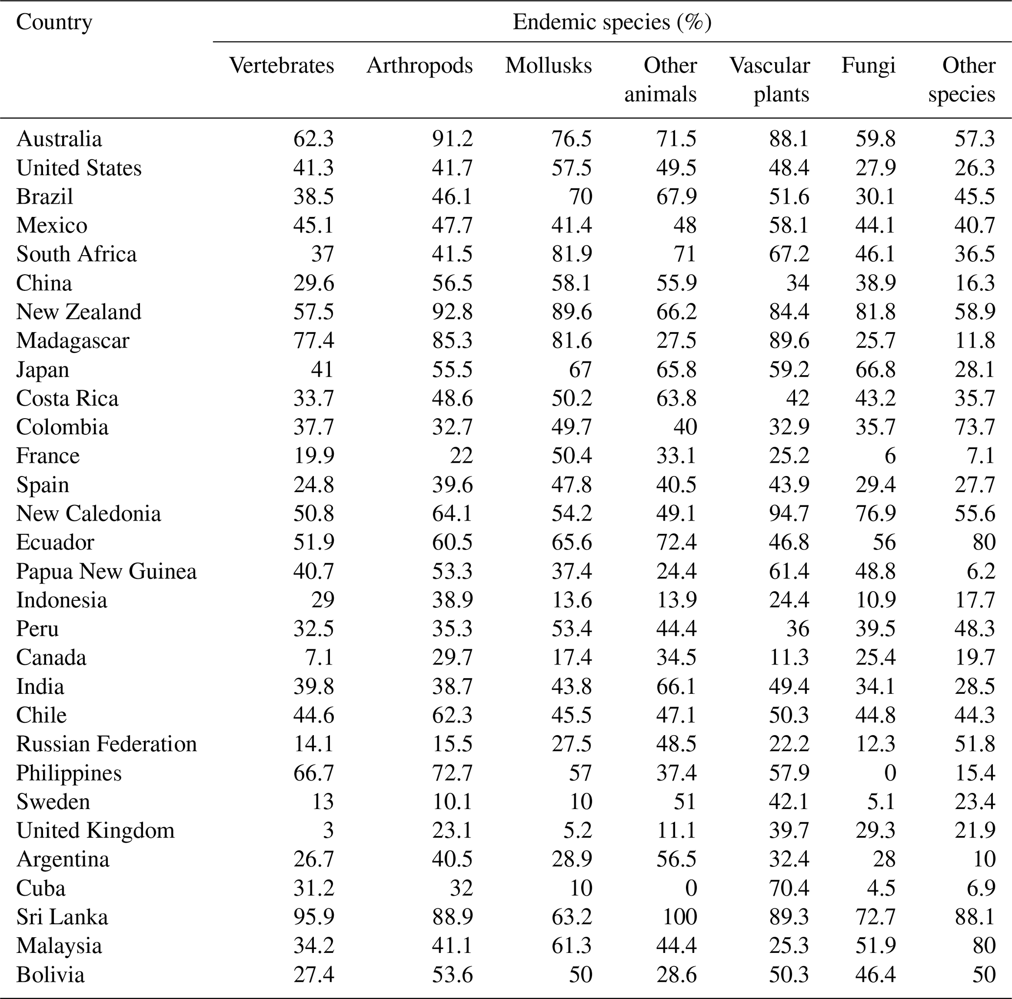
It should be noted that Table 2 excludes small island territories that rank high in at least one group, including South Georgia, French Polynesia, Heard and McDonald Islands, Norfolk Island, and the Malvinas/Falklands non-determined legal status territory.

4.2 Distribution of small-region species

Small range size has been studied extensively in the empirical literature (Jenkins et al., 2015; Kraus et al., 2023; Manne et al., 1999; Manne and Pimm, 2001; Purvis et al., 2000; Veach et al., 2017). Jenkins et al. (2015), for example, note that “small range size is the best predictor of extinction risk and, thus, the first metric for conservation priority.” It has particular significance since it is a widely recognized indicator of extinction risk that is computable for any species that can be mapped.

However, it should be noted that small-range status is not determinate; there is no single, critical minimum habitat size, given the myriad interactions between species and habitat characteristics that affect extinction risks. Therefore, we examined the size and global distribution of species with small occurrence regions in our GBIF maps database, considering the effects of changing the criteria for small-occurrence-region status. Table 3 displays the cumulative global count for species groups as the occurrence region increases from 5 km × 5 km to 200 km × 200 km. Even for occurrence regions of 10 km × 10 km or less, 57 765 species are identified; this number increases to 85 310 at 25 km × 25 km or less. Differences across species groups reflect their varying representation in the database and group-specific factors.

Table 3 Species counts by group and grid scale.

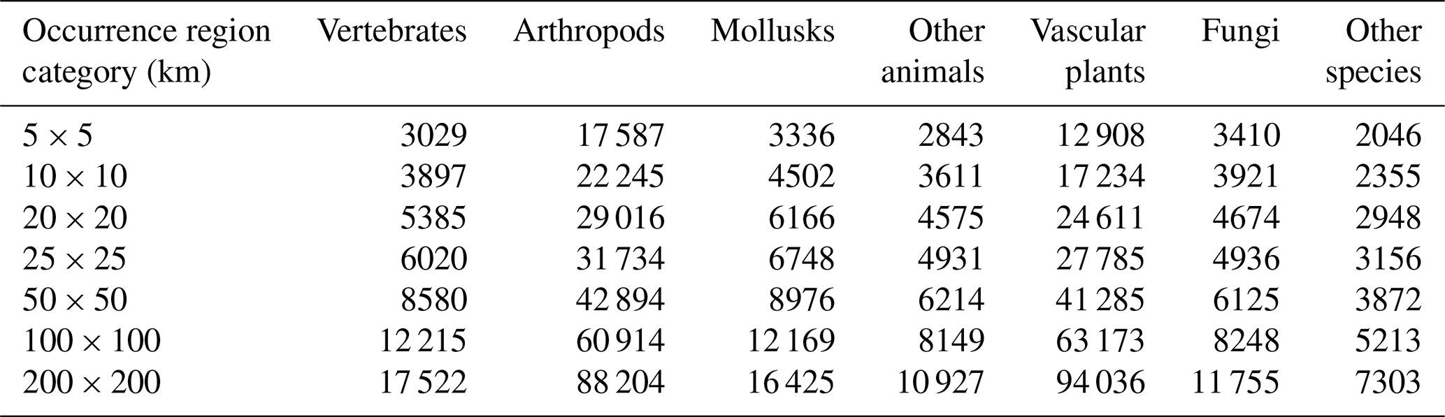
We believe that an upper bound of 25 km × 25 km on a critical scale for small-range species is appropriately conservative. The small-range species count increases to 117 946 at 50 km × 50 km or less, 170 081 at 100 km × 100 km or less, and 246 172 at 200 km × 200 km. From a policy perspective, the feasibility and sustainability of species protection tend to decline as the number of species protected increases. Since even the 25 km × 25 km limit qualifies nearly 85 310 species as having a small occurrence region, we retain it here, recognizing that other analyses may well opt for higher limits.

Using GIS overlays of GBIF maps and country boundaries, we count species with small occurrence regions by country, finding that their international distribution is skewed. The top 30 countries account for 75.5 % of them (64 443 out of 85 310 species). Our overall results assign top 10 status to Australia, United States, Brazil, Mexico, France, South Africa, Costa Rica, China, Colombia, and Japan. Australia leads with 8673 species, followed by the United States (7791), Brazil (4434), Mexico (4217), and France (3732). Comparing Table 3 with Table 4 suggests that small-occurrence-region species are endemic in most cases, so the dominant country is chosen by default. In other cases (e.g., Panama, Venezuela, RB, Thailand, and Italy), it is the country with greatest area share in the species' GBIF occurrence map. Among species groups, the top 30 countries' global share varies from 66 % (vertebrates) to 78 % (arthropods) (Table 4).

Table 4 Top 30 countries for species with small occurrence regions, by group.

4.3 Distribution of endemic species with small occurrence regions

We also explored the geographical distribution of endemic species with small occurrence regions (25 km × 25 km size limit). Our results identified 67 941 species in a single country (Table 5).

Table 5 Top 30 countries for endemic species with small occurrence regions, by group.

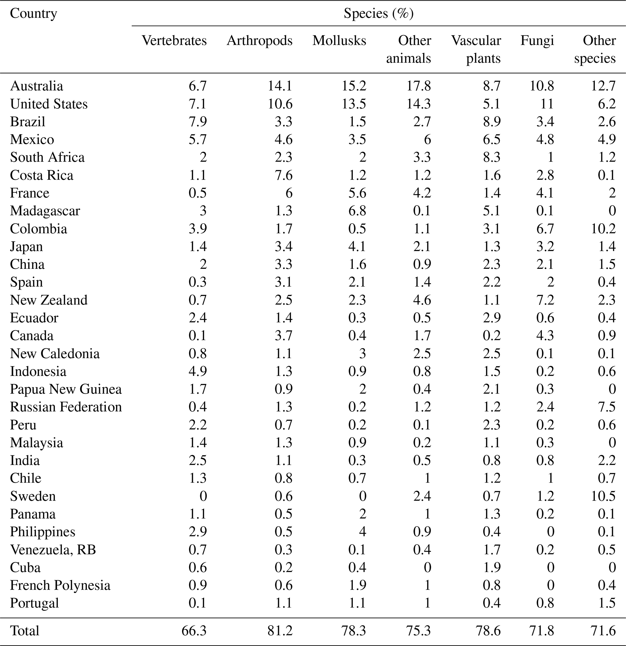
As before, we find that the international distribution is skewed, with 78.2 % (53 114) of the 67 941 species found in 30 countries. The overall results assign top 10 status to Australia, United States, Brazil, Mexico, South Africa, Costa Rica, France, Madagascar, Colombia, and Japan. Australia leads with by 8072 species, followed by the United States (6003), Brazil (3629), Mexico (3621) and South Africa (2911). Among species groups, the top 30 countries have the following global shares: arthropods (81.2 %), vascular plants (78.6 %), mollusks (78.3 %), other animals (75.3 %), fungi (71.8 %), other non-animal and non-plant species (71.6 %), and vertebrates (66.3 %).

Among endemic species with small occurrence regions, the largest share is found in Oceania (28 %), followed by North America (23 %). Four regions are in the mid-range – South America (15 %), Asia (13 %), Africa (11 %), and Europe (9 %) – and Antarctica has small representation, at 1 % (Fig. 6).

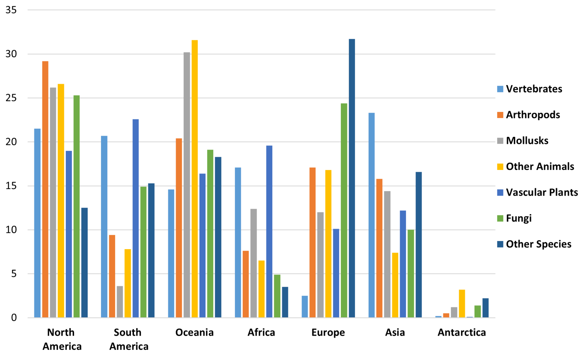
Figure 6 Regional distribution (percentage) of endemic species with small occurrence regions.

4.4 Candidate hotspot areas for protection

Limited resources for biodiversity conservation make it critical to prioritize protection efforts in regions inhabited by many unique, at-risk species. Endemism and small occurrence regions, as identified by our maps, can inform conservation policy priority-setting. This study's findings indicate that 40 countries have significant opportunities for protecting areas with concentrations of endemic species, species with small occurrence regions, and species with both features. Aligning countries with World Bank income groups reveals an encouraging trend for conservation. While over 4000 endemic species with small ranges are in Low- and Lower-Middle-Income countries, the majority, 82.7 %, are in high and upper-middle-income countries (Fig. 7), which generally have substantial conservation resources. Many such areas may already be protected. Although a global assessment was beyond this study's scope, it would be a valuable future application of our GBIF species maps database.

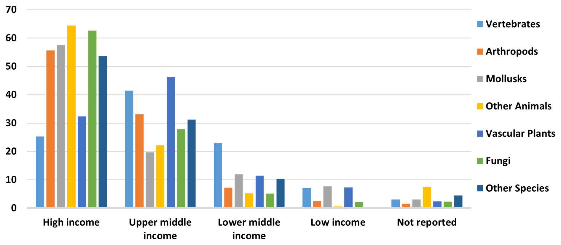
Figure 7 Percent distribution of endemic species with small occurrence regions, by income class.

It should be noted that the maps constructed with processed data also provide opportunities for understanding the geographic distribution of the species within countries.

5 Discussion

Transparent and accessible biodiversity data remain central to informed decision-making for conservation and to safeguarding a livable planet for current and future generations. However, comprehensive and all-taxa-inclusive biodiversity data have long been scarce, limiting the ability to assess species distribution and conservation priorities at a global scale. This study presents the first near-comprehensive global mapping of terrestrial, freshwater, and marine biodiversity derived from GBIF occurrence data. By applying the alphahull algorithm and complementary clustering techniques to over 600 000 species, the analysis demonstrates that high-resolution, occurrence-based approaches provide a robust complement to expert-drawn range maps. Building on these results and given the numerous competing demands on land and water, the spatial precision of conservation activities and policies can be enhanced through alphahull techniques, thereby increasing their potential for success by effectively focusing the area of consideration. Also, our effort aligns with that of Janicki et al. (2016), and a salient contribution of this work is the inclusion of previously unmapped taxa – particularly invertebrates, fungi, and plants – which substantially broadens the taxonomic and spatial scope of global biodiversity representation.

5.1 Expanding the biodiversity evidence base

The observed alignment between occurrence-based and expert-derived maps underscores the potential of crowdsourced georeferenced data for large-scale biodiversity mapping. Discrepancies between the two primarily reflect temporal and ecological scope. Expert maps typically represent potential distributions based on habitat suitability and species ecology, while occurrence-based maps capture realized distributions shaped by recent environmental and anthropogenic dynamics (Meyer et al., 2016). Consequently, GBIF-derived boundaries can more effectively detect recent range contractions or expansions associated with deforestation, climate change, or land-use conversion. The rapid updating of GBIF records – currently exceeding one million new georeferenced occurrences daily – creates opportunities for near-real-time monitoring of biodiversity change, a capability unavailable in static expert compilations.

5.2 Addressing taxonomic and geographic bias

A major contribution of this work lies in filling taxonomic gaps that have historically constrained global biodiversity assessments. Existing global datasets emphasize vertebrates, overlooking invertebrates and fungi that together comprise the majority of known species (Cardoso et al., 2011). The integration of over 213 000 arthropods, 38 000 fungi, and 24 000 other animal taxa demonstrates the feasibility of incorporating these groups systematically into global-scale analyses. While GBIF data remain spatially biased toward accessible and high-income regions (Yesson et al., 2007), ongoing growth in citizen science platforms and institutional data sharing is steadily improving geographic representativeness. As observation density increases, particularly across tropical and remote regions, boundary estimation will gain precision, enabling more accurate identification of small-range and data-poor species.

5.3 Implications for conservation priority setting

The identification of endemic and small-range species from GBIF-derived maps provides new insights for conservation targeting. A broader view of biodiversity provides an opportunity for more countries to contribute to a shared vision of conservation stewardship, as most nations host significant distributions of species within at least one major taxonomic group. Consistent with prior studies (Kier et al., 2009), this analysis confirms that small-range species are disproportionately at risk of extinction due to limited dispersal capacity and habitat specialization. The correlation between endemism and small-range occurrence suggests that national-level conservation actions will be critical for achieving global biodiversity outcomes. Australia, the United States, Brazil, Mexico, and South Africa emerge as global centers of endemism and small-occurrence-region species, underscoring their unique biodiversity assets. The identification of numerous localized hotspots – such as Madagascar, Costa Rica, and Southeast Asia – further highlights regions where protection gap analyses are most urgent.

5.4 Policy relevance and the Global Biodiversity Framework

Implementing the goal of protecting 30 % of the planet's land and sea areas by 2030, as set out in Target 3 of the 2022 Kunming–Montreal Global Biodiversity Framework (GBF), requires precise identification of areas critical for conservation. Using occurrence data for over 600 000 species from GBIF, this study provides the largest set of species distribution maps derived from open-access data and highlights 30 countries that could play central roles in area-based conservation, capturing 86.6 % of endemic species, 75.5 % of small-occurrence-region species, and 78.2 % of species that are both endemic and range-limited. These data can also be used to examine the overlap of existing protected areas with endemic-species distributions, highlighting significant variation in initial conservation conditions, including current protection levels and the spatial distribution of unprotected species (Dasgupta et al., 2025a, b).

The GBIF database, expanding by approximately 1.3 million new records daily, allows continuous updates for previously unmapped species and refinement of existing maps. The estimation algorithm supports this growth, providing area estimates for all species and complementing traditional risk indicators. In addition, the alpha hull approach offers a parsimonious, occurrence-driven estimate of species range, requiring minimal assumptions and no environmental predictors. Our practical experience in client countries further indicates that communicating with policymakers is often more straightforward when using species occurrence regions derived from reported occurrences, compared to statistical modeling methods that infer occurrence from environmental predictors, which can be challenging to explain. Given the rate of biodiversity loss, it is urgent to initiate the biodiversity dialogue immediately, beginning with approaches to mapping that are readily understandable. The open-access nature of the data, algorithms, and maps aligns with the GBF's emphasis on equitable sharing, transparency, and evidence-based policy design. High-resolution, taxonomically inclusive maps can guide national and transboundary prioritization, while continuous updating allows adaptive policy responses – an essential feature for tracking progress toward GBF targets and ensuring accountability in biodiversity monitoring frameworks. This need for spatially explicit and scalable information is particularly relevant for international institutions and development organizations. An information paradox often confronts decision-makers in transnational institutions: while the scope of their operations is global, the scale of specific interventions is inevitably local or regional (Blankespoor et al., 2023).

Looking ahead, open and equitable sharing of biodiversity, threat, and protection data across administrative boundaries remains essential, as species and ecosystems frequently span political jurisdictions (Blankespoor et al., 2025; Dasgupta et al., 2025c; Tanalgo, 2025). Reliable, high-resolution, and up-to-date data facilitate coordinated conservation strategies across terrestrial, freshwater, and marine systems. Healthy biodiversity underpins ecosystem stability and sustains essential services such as agriculture, fisheries, water security, and climate resilience. It is therefore fundamental to sustainable development, poverty alleviation, equitable prosperity, and safeguarding a livable planet for current and future generations.

5.5 Limitations and future directions

Despite these advances, several limitations warrant acknowledgment. First, GBIF occurrence data remain uneven in spatial and temporal coverage, with collection bias favoring regions with established research infrastructure, accessibility and funding (Beck et al., 2014; Boakes et al., 2010; Hickisch et al., 2019; Faxon and Chapman, 2025). Hortal et al. (2015) discuss shortfalls of biodiversity data including taxonomic (Linnean), distribution (Wallacean), and abundance (Prestonian). First, taxonomic challenges can persist because research effort is often linked to a disproportionate concentration on early-described taxa, as in the case of 10 000 reptile species examined by Guedes et al. (2023). In a study of the Eastern Arc Mountains in Tanzania, Ahrends et al. (2011) find suggestive evidence of biodiversity patterns linked with investment in inventories. Second, accurate species occurrence records are needed to improve the understanding of species distribution mitigating the “Wallacean Shortfall.” Third, presence-only data do not capture species abundance, which limits inference about population viability within mapped boundaries. Fourth, while the alphahull method provides an efficient means of delineating occurrence extents, it does not explicitly account for environmental suitability or ecological connectivity. Future research could enhance these methods by integrating species distribution modeling, remote-sensing covariates, sampling, latitudinal taxonomic gradient and temporal updating to capture dynamic species–environment interactions (Elith and Leathwick, 2009; Diniz-Filho et al., 2023).

Although GBIF strengthens the data ecosystem providing a common repository for data collections from scientists, agencies, community science and museums (Heberling et al., 2021), further investment would help improve GBIF completeness by building local digitization and curation capacity and by integrating diverse data streams. Empirical work in the Amazon illustrates both the promise and challenges of current approaches: de Araujo et al. (2022) find that combining global and national databases can increase biodiversity knowledge and reduce inventory gaps. Sustained efforts to digitize, publish, and improve data quality are essential for keeping biodiversity data efficient, effective, and relevant (Ball-Damerow et al., 2019). Targeted capacity-building programs, such as GBIF's Biodiversity Information for Development (BID), support data mobilization, training, and publisher engagement to improve the coverage and usability of biodiversity data across the world (GBIF, 2025).

6 Code and data availability

These data are available at the World Bank's Development Data Hub under Global Biodiversity Species Occurrence Gridded Data and Global Biodiversity Species Occurrence Endemism and Small Range Data. The datasets can be accessed at https://doi.org/10.57966/h21e-vq42 (Dasgupta et al., 2024). The authors utilized Google BigQuery to retrieve species occurrence records and R software for data processing. The associated scripts are available from the authors upon request. Appendix B includes a flowchart of the main processing algorithm.

7 Concluding Remarks

Overall, this study demonstrates the feasibility and scientific value of automated, open-access biodiversity mapping at global scale. By complementing expert-based datasets with data-driven, continuously updatable occurrence maps, it bridges long-standing taxonomic and geographic data gaps, improves spatial precision for conservation planning, and enhances the policy relevance of biodiversity information systems. As global data sharing and digital observation platforms continue to expand, the approach outlined here can provide a scalable and transparent foundation for evidence-based implementation of the Global Biodiversity Framework and related multilateral environmental agreements.

Appendix A

A1 Case Comparisons of Species Occurrence Regions and expert maps

To test our species boundary mapping from the current inventory, we compare the global biodiversity patterns derived from our current inventory with those depicted in expert-generated maps. By aligning our GBIF-based occurrence maps with expert maps from recent studies, we identify thousands of overlapping species. These shared species serve as the basis for assessing how closely our GBIF-derived biodiversity patterns match those reported in the expert research.

We compare our Species Occurrence Regions derived from GBIF with the sets of matched species for mammals (Marsh et al., 2022), ants (Kass et al., 2022) and plants (Borgelt et al., 2022) with a confusion matrix with 5 to 10 classes by distribution (see Table A1). Model performance varied across taxa and the number of classes. For mammals, overall accuracy was highest at 0.452 (κ = 0.315) with 5 classes to the lowest at 0.263 (κ = 0.181) with 10 classes, indicating that model agreement beyond chance declined as class complexity increased. Ants showed slightly higher performance at low class counts, with accuracy of 0.501 (κ = 0.374) for 5 classes, dropping to 0.311 (κ = 0.234) for 10 classes. Plants were the best-predicted group, achieving 0.673 accuracy (κ = 0.591) for 5 classes and 0.450 accuracy (κ = 0.389) for 10 classes. Across all taxa, accuracy confidence intervals were narrow, reflecting precise estimates, and all comparisons were significantly better than random (Accuracy p-value = 0). These results suggest that predictive performance declines with increasing class granularity, with plants consistently outperforming ants and mammals in overall accuracy and agreement.

We also produce maps of the differences in ranks between our GBIF-based occurrence maps with the expert maps. We illustrate three categories: (i) GBIF has a lower rank than expert map by more than 2 ranks, (ii) similar rank that includes an absolute difference of 2 ranks or fewer and (iii) GBIF has a higher rank than the expert map by more than 2 ranks (see Fig. A1 for matched mammals, Fig. A2 for full mammals, Fig. A3 for plants and Fig. A4 for ants).

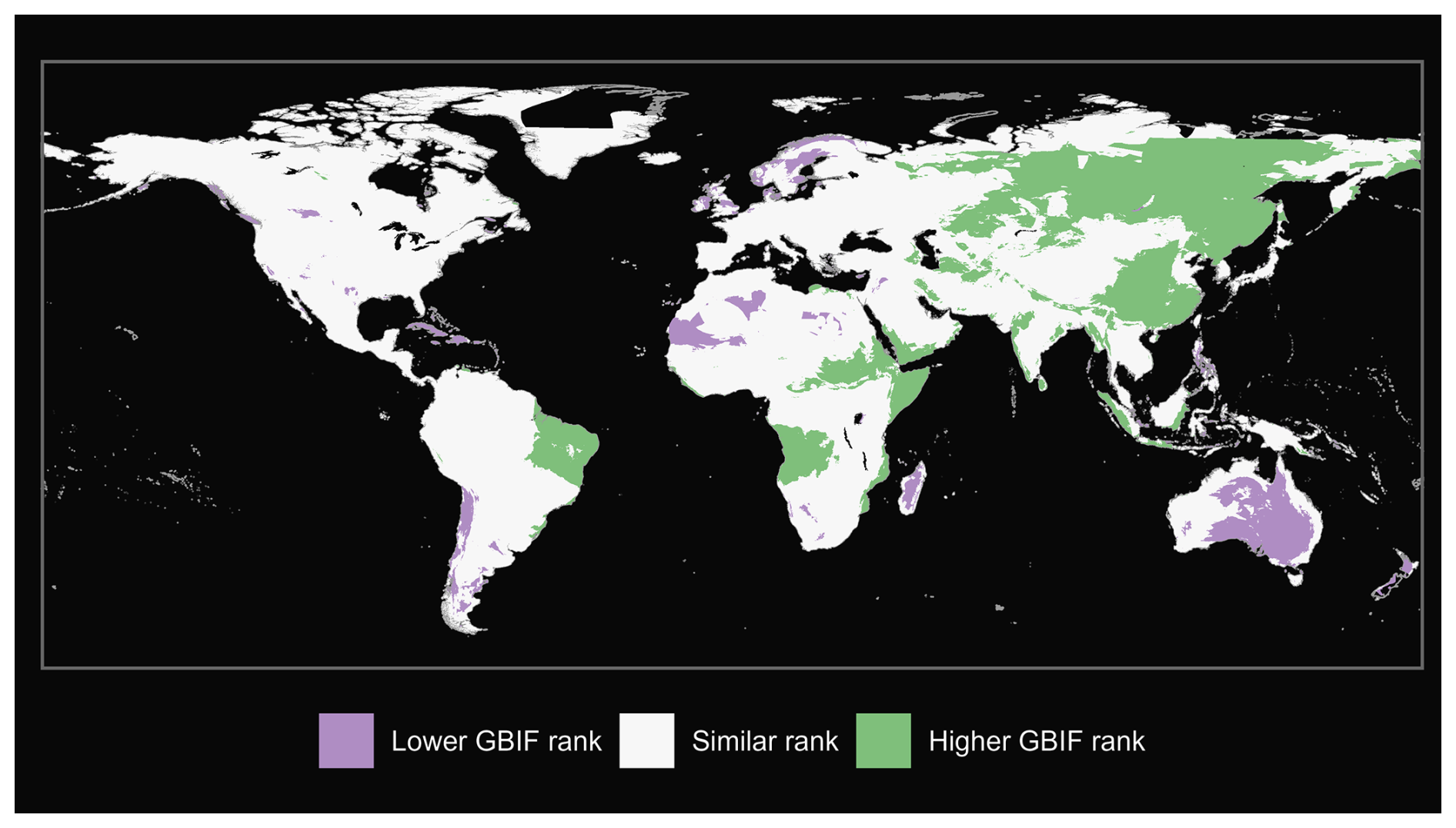
Figure A1 Comparison of matched mammals from our GBIF species occurrence regions and expert-based map (Marsh et al., 2022).

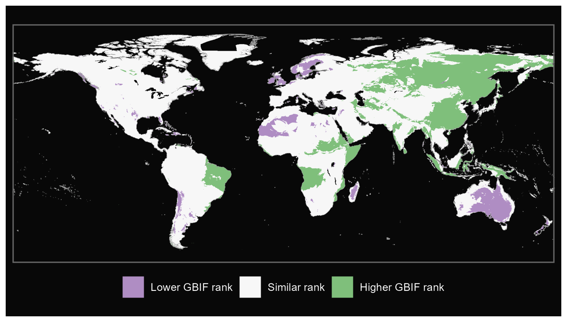
Figure A2 Comparison of full mammals from our GBIF species occurrence regions and expert-based map (Marsh et al., 2022).

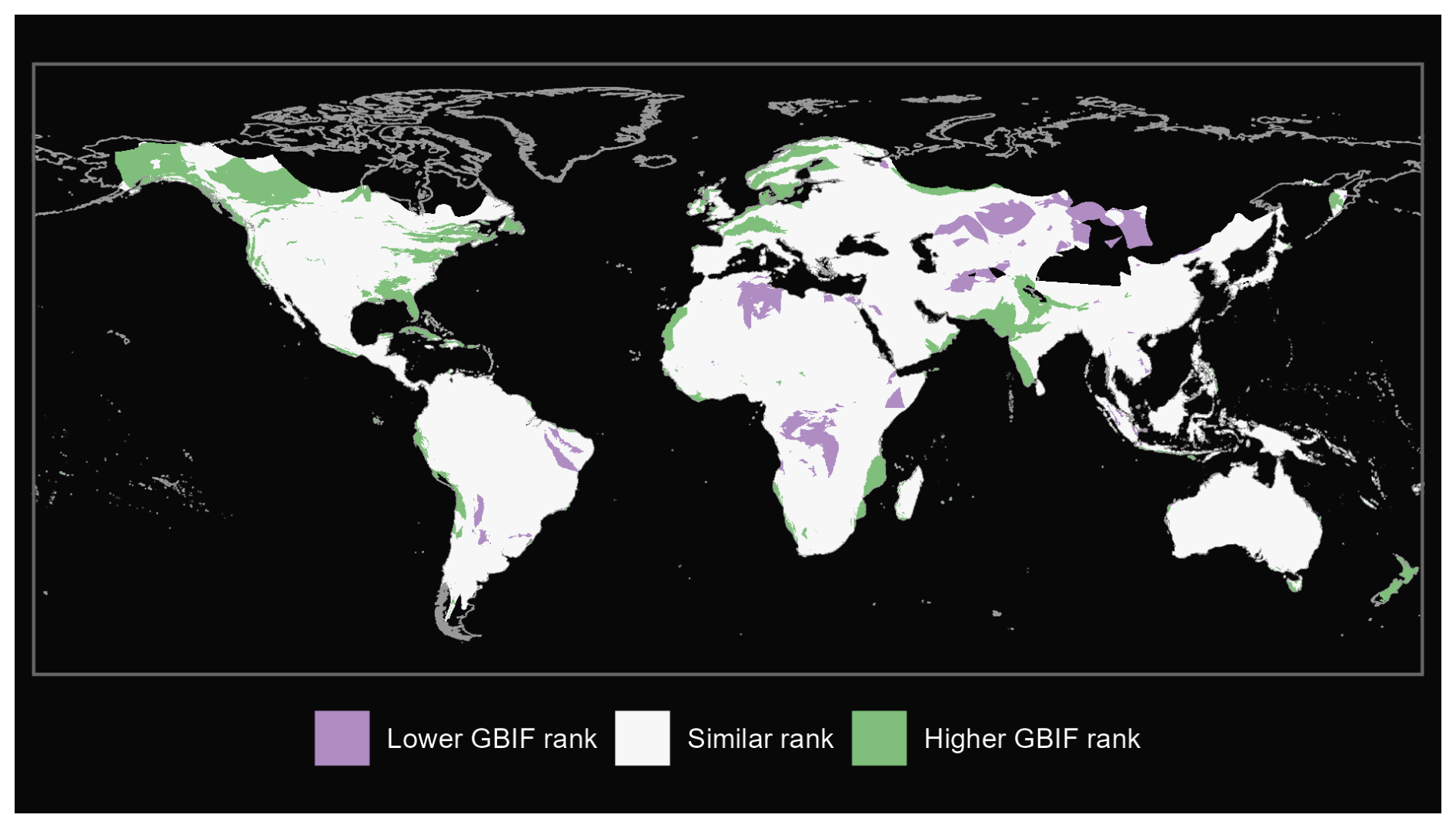
Figure A3 Comparison of ants from our GBIF species occurrence regions and expert-based map (Kass et al., 2022).

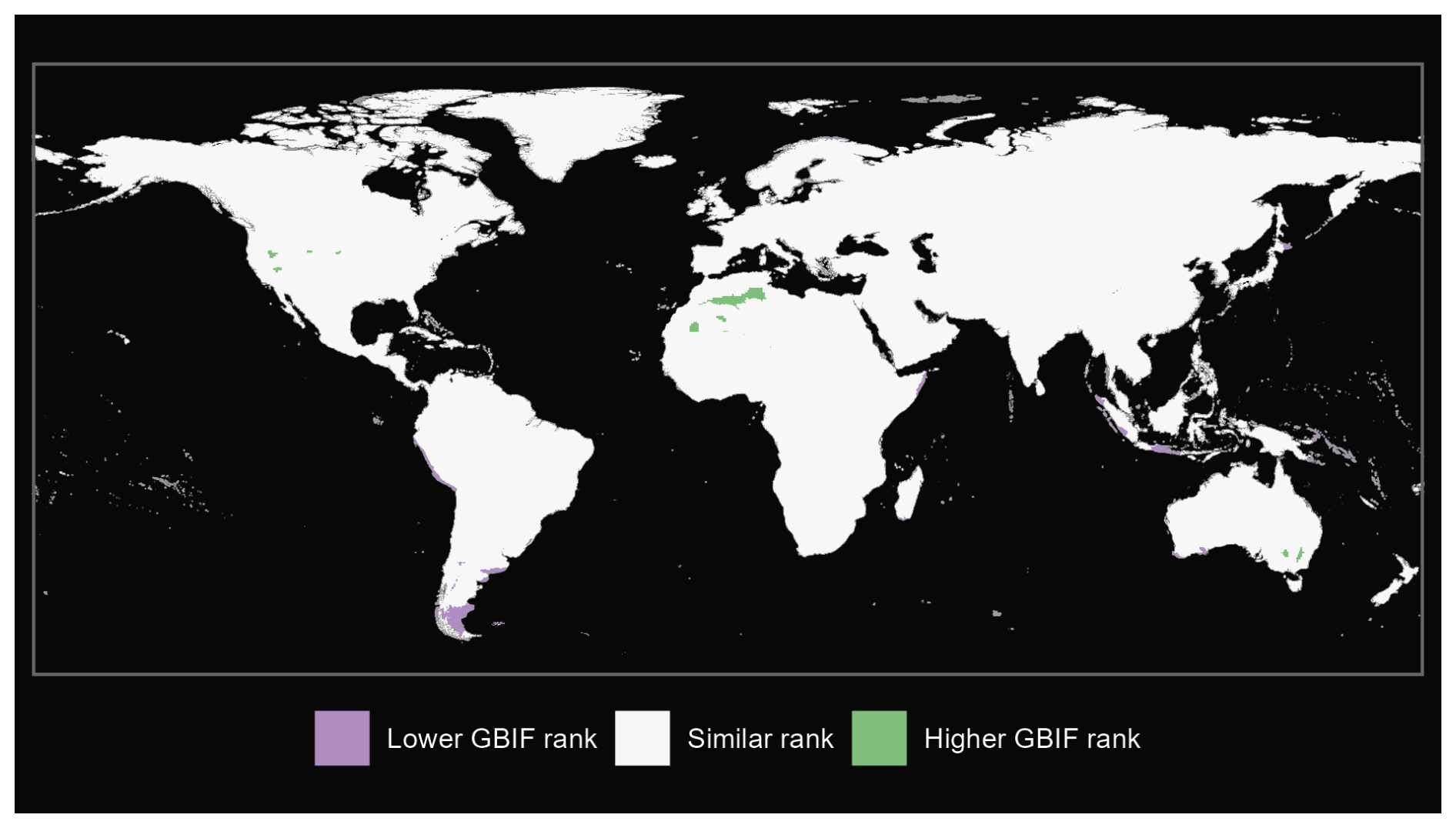
Figure A4 Comparison of plants from our GBIF species occurrence regions and expert-based map (Borgelt et al., 2022).

A2 Case Comparisons of Species Occurrence Regions and expert maps

To evaluate differences between spatial modeling approaches, we compared species occurrence regions generated using the convex hull and alpha hull methods across representative taxa, including arthropods, birds, fungi, fish, plants, and reptiles. The convex hull method defines a minimal polygon encompassing all occurrence points, while the alpha hull identifies finer boundaries that can separate spatially distinct clusters (see Sect. 2.2). Table A2 provides the area for each method and the ratio of convex hull area over alpha hull area. Species groups are discussed below with maps of selected species.

A2.1 Arthropods

For arthropods, we examined Thermocyclops neglectus, a species broadly distributed across Africa. The convex hull method delineated a large area of approximately 5.50 million km², encompassing the full extent of known occurrences. In contrast, the alpha hull produced two distinct clusters totaling 0.213 million km², representing only about 3 % of the convex hull extent (ratio = 25.89). This result illustrates how the alpha hull approach captures core occurrence zones more precisely while excluding large intervening areas of apparent absence (Fig. A5).

Table A1 Model Accuracy and Kappa across case comparisons.

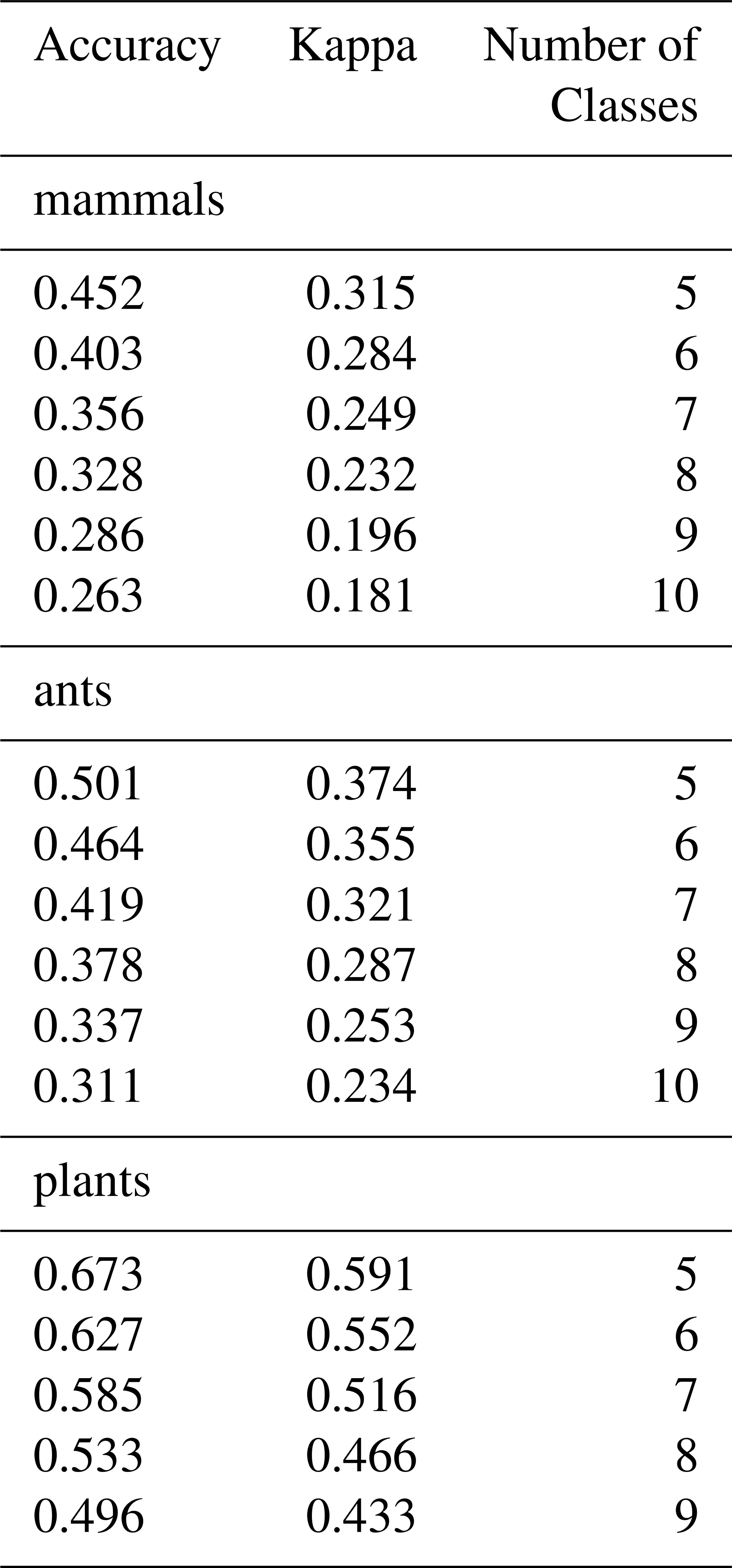
Table A2 Selected species with comparison of convex hull and alpha hull results.

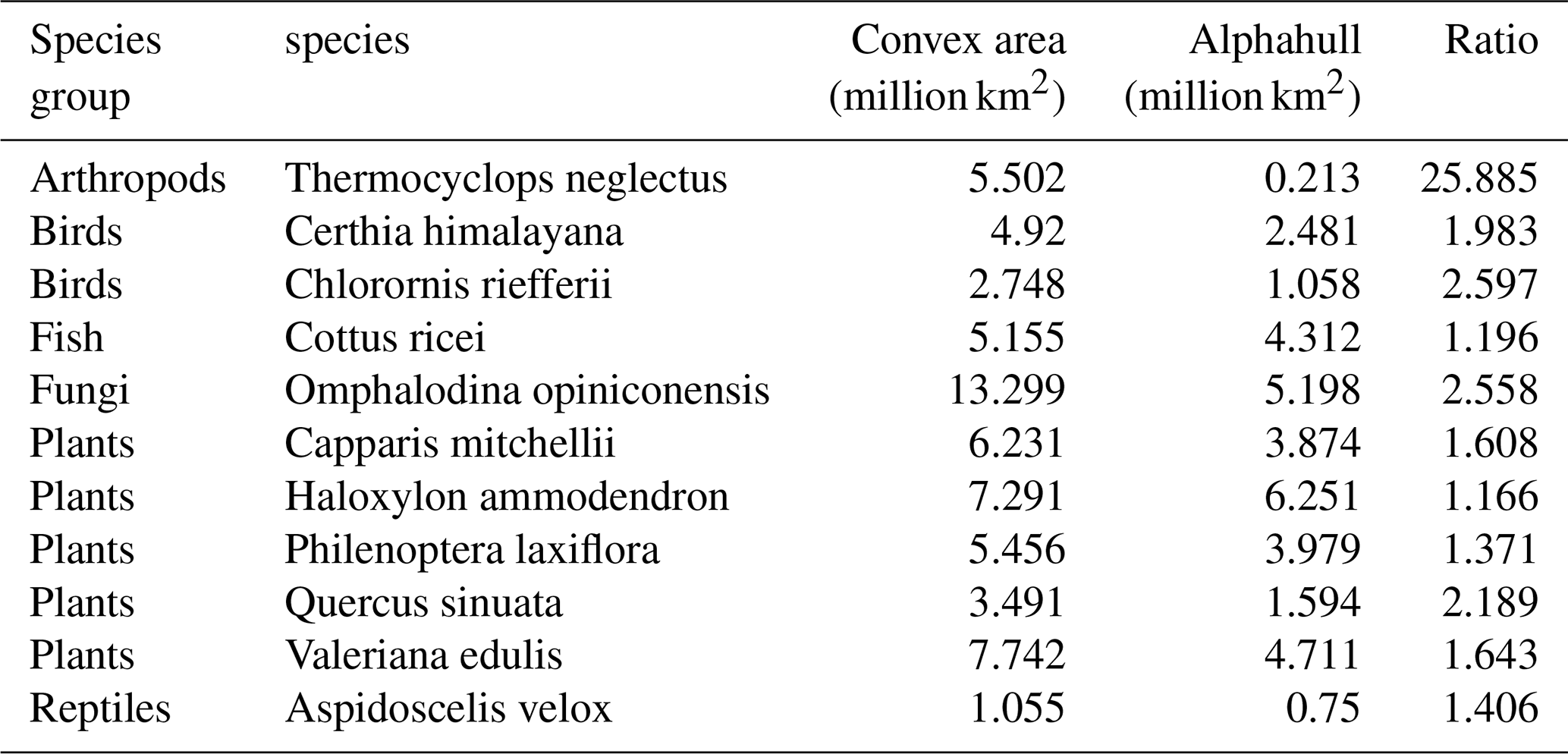
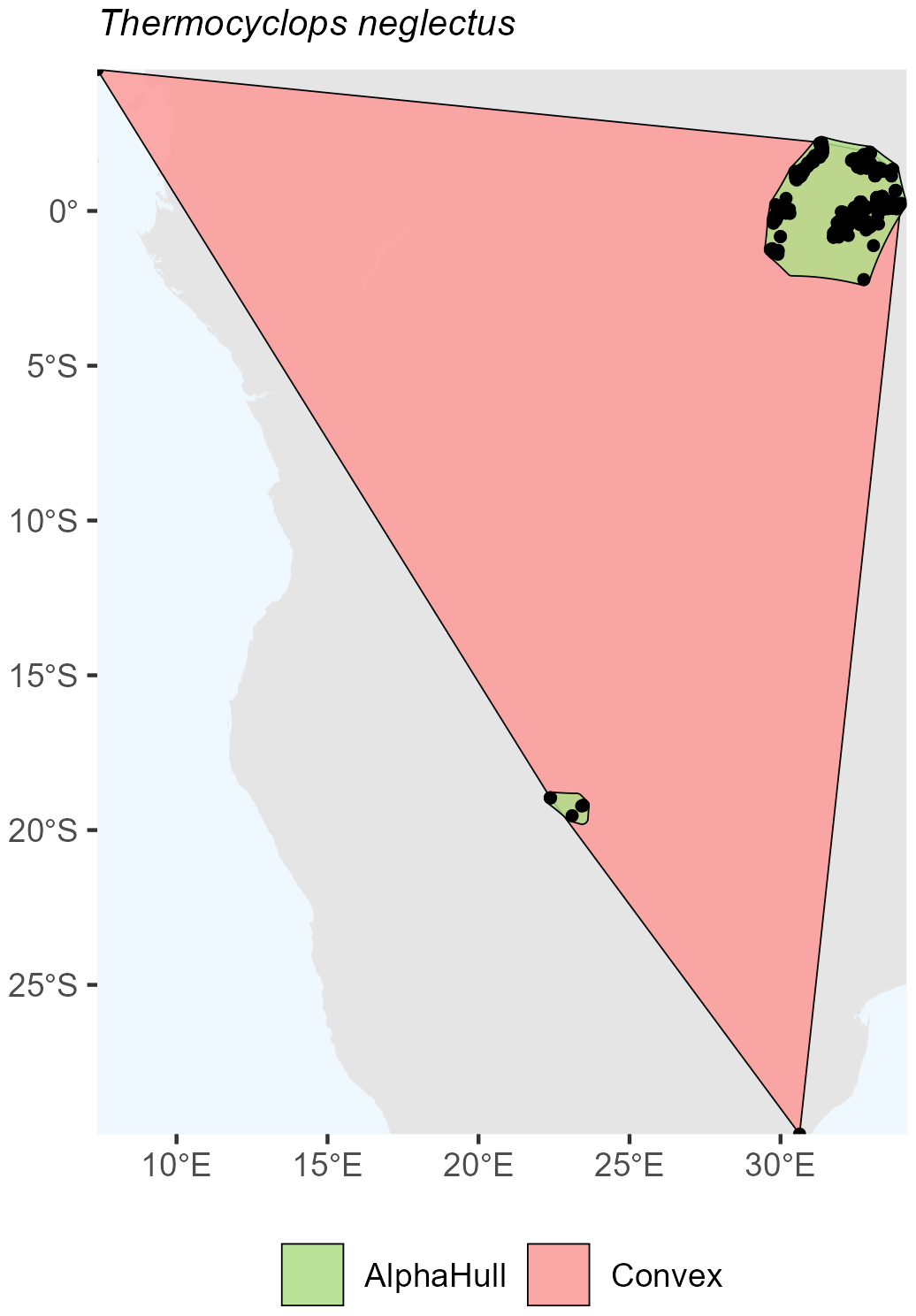
Figure A5 Species occurrence region of Thermocyclops neglectus.

A2.2 Birds

Among birds, we selected Certhia himalayana and Chlorornis riefferii, which represent species with relatively continuous and moderately fragmented distributions, respectively. For Certhia himalayana found in Asia, the convex hull area (4.9 million km²) was about twice as large as the alpha hull area (2.5 million km²), yielding a ratio of 1.98, indicating moderate spatial refinement by the alpha hull (Fig. A6). Chlorornis riefferii found in South America showed a slightly higher ratio (2.60), suggesting more fragmented or discontinuous occurrence points, where the alpha hull excluded peripheral areas of low density (Fig. A7).

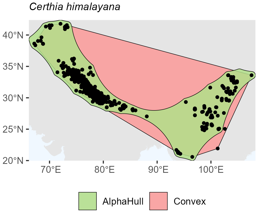
Figure A6 Species occurrence region of Certhia himalayana.

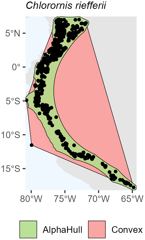
Figure A7 Species Occurrence Region of Chloronis riefferii.

A2.3 Fish

For the freshwater fish Cottus ricei found in North America, the convex hull encompassed an area of 5.16 million km², only modestly larger than the alpha hull estimate (4.31 million km², ratio 1.20) (Fig. A8). This relatively low ratio indicates a spatially cohesive set of occurrence records, with both hull methodsapturing a similar extent of distribution.

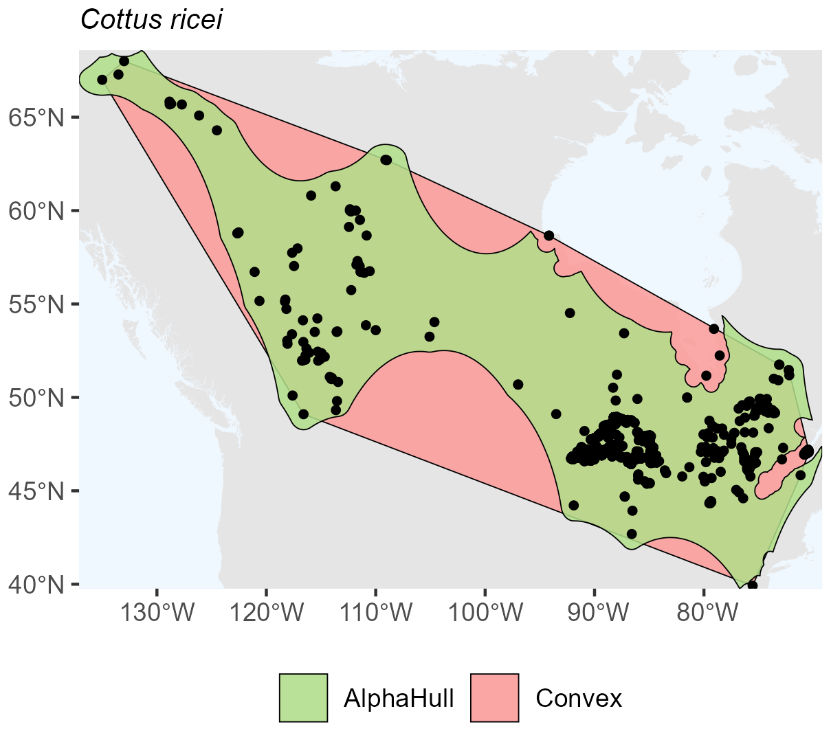
Figure A8 Species Occurrence region of Cottus ricei.

A2.4 Fungi

In fungi, the species occurrence regions of Omphalodina opiniconensis show a broad North American distribution, with the convex hull covering 13.3 million km² and the alpha hull reducing this to 5.2 million km² (ratio 2.56) (Fig. A9). This pattern suggests that while the species is widespread, its occurrences form distinct spatial clusters that the alpha hull captures more precisely, excluding large unoccupied areas within the convex hull boundary.

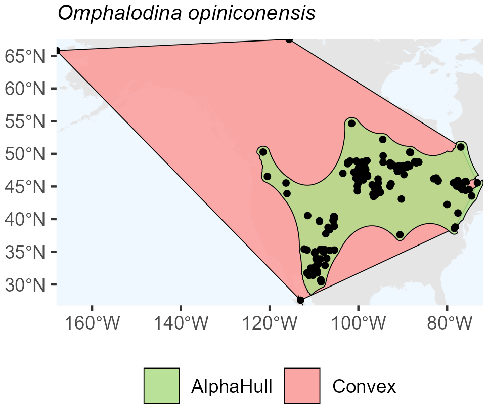
Figure A9 Species Occurrence Region of Omphalodina opiniconensis.

A2.5 Plants

Five plant species were analyzed, showing variable differences between the two methods.

Capparis mitchellii, which is native to Australia, (ratio 1.61) and Philenoptera laxiflora, which is found across Africa, (ratio 1.37) both exhibited moderate spatial contraction under the alpha hull, indicating relatively continuous distributions with some peripheral refinement (Figs. A10 and A11, respectively).

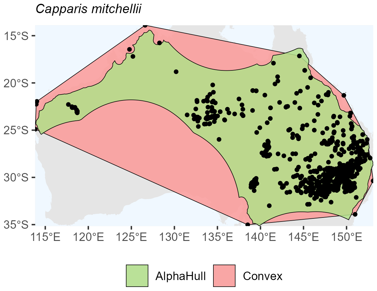
Figure A10 Species Occurrence Region of Capparis mitchellii.

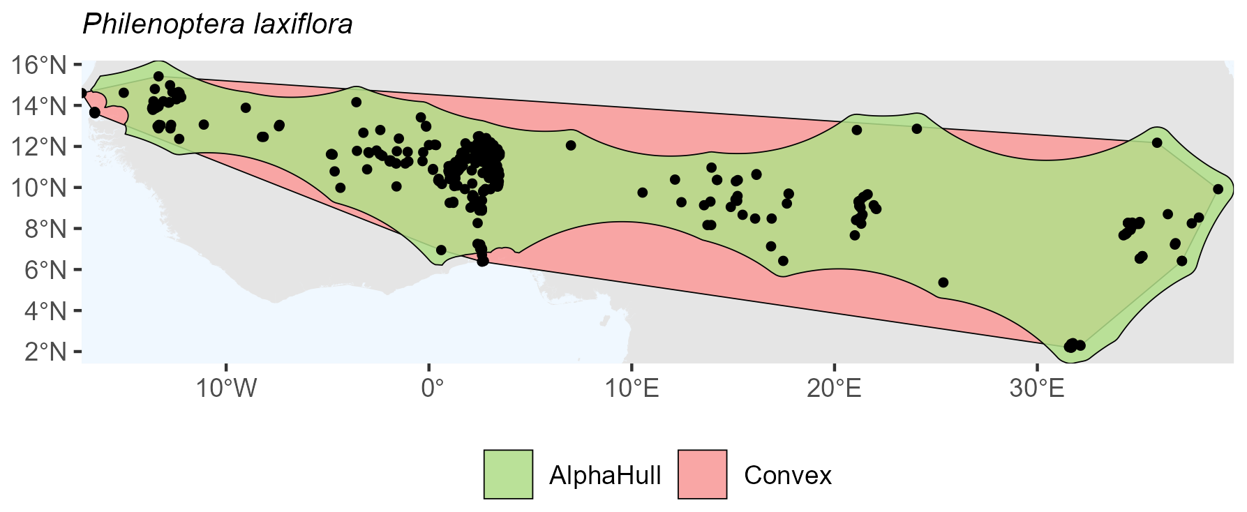
Figure A11 Species Occurrence Region of Philenoptera laxiflora.

Haloxylon ammodendron, which is found in Asia, showed minimal difference (ratio 1.17), suggesting a dense and cohesive set of occurrences across its range (Fig. A12).

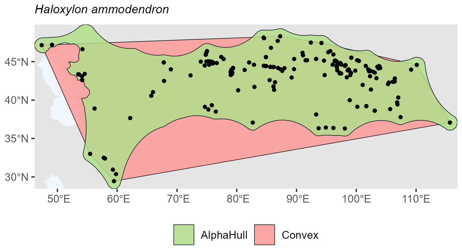
Figure A12 Species Occurrence Region of Halosylon ammodendron.

Quercus sinuata, which is found in North America (ratio 2.19) (Fig. A13), and Valeriana edulis, also found in North America (ratio 1.64), had higher ratios, pointing to patchier occurrence patterns or geographic discontinuities (Fig. A14).

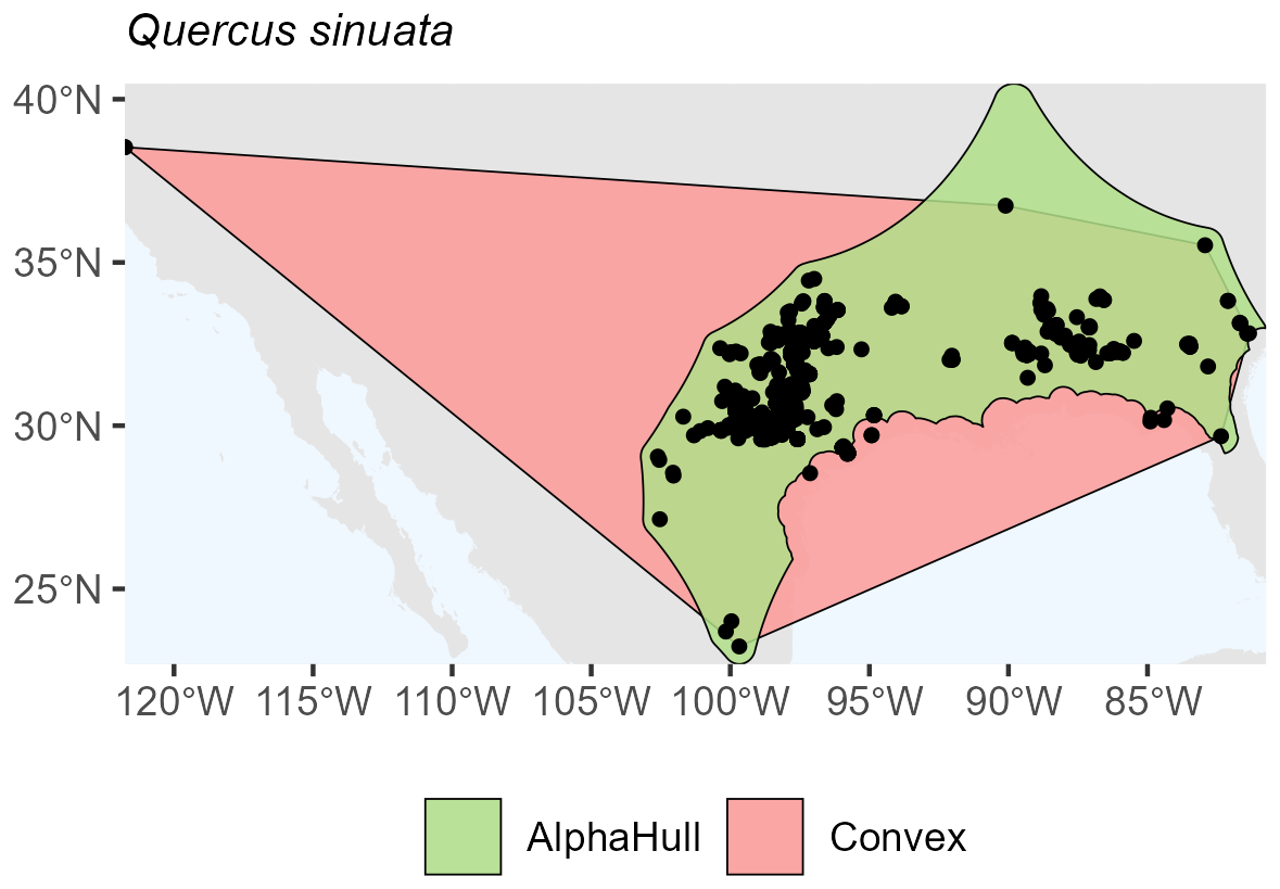
Figure A13 Species Occurrence Region of Quercus sinuata.

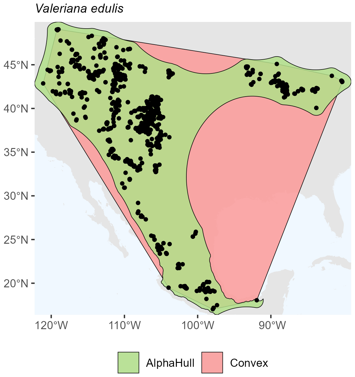
Figure A14 Species Occurrence Region of Valeriana edulis.

Overall, the plant species showed consistent trends where the alpha hull excluded peripheral gaps, providing a more ecologically realistic boundary.

A2.6 Reptiles

For reptiles, the species Aspidoscelis velox, which is found in North America, showed a convex hull area of 1.06 million km²compared to 0.75 million km² from the alpha hull (ratio 1.41) (Fig. A15). This moderate difference reflects a relatively compact but slightly fragmented distribution.

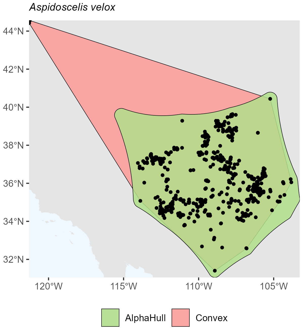
Figure A15 Species Occurrence Region of Aspidoscelis velox.

Across all taxa, convex hull areas consistently exceeded those derived from alpha hulls, as expected from their respective geometric definitions. The convex hull to alphahull area ratios ranged from 1.17 (H. ammodendron) to 25.89 (T. neglectus), reflecting the degree of spatial clustering among occurrence records. The extreme difference observed for T. neglectus highlights the alpha hull's ability to delineate discrete occurrence clusters and avoid overestimation of occurrence region. Collectively, these findings demonstrate that while convex hulls provide rapid, broad-range approximations, alpha hulls yield finer, more ecologically meaningful representations of species distributions, particularly for taxa with spatially discontinuous occurrences.

From a policy perspective, the results highlight a pattern where convex hull produces areas that are much larger than where the clusters of species occurrences are located. Since there are many competing demands for land and water, the potential success of conservation activities/policy are more precise (spatially) using the alphahull techniques as it focuses the area of consideration.

Appendix B: Flowchart of the main processing algorithm

Figure B1 Flowchart summary of the processing method for Species Occurrence Regions.

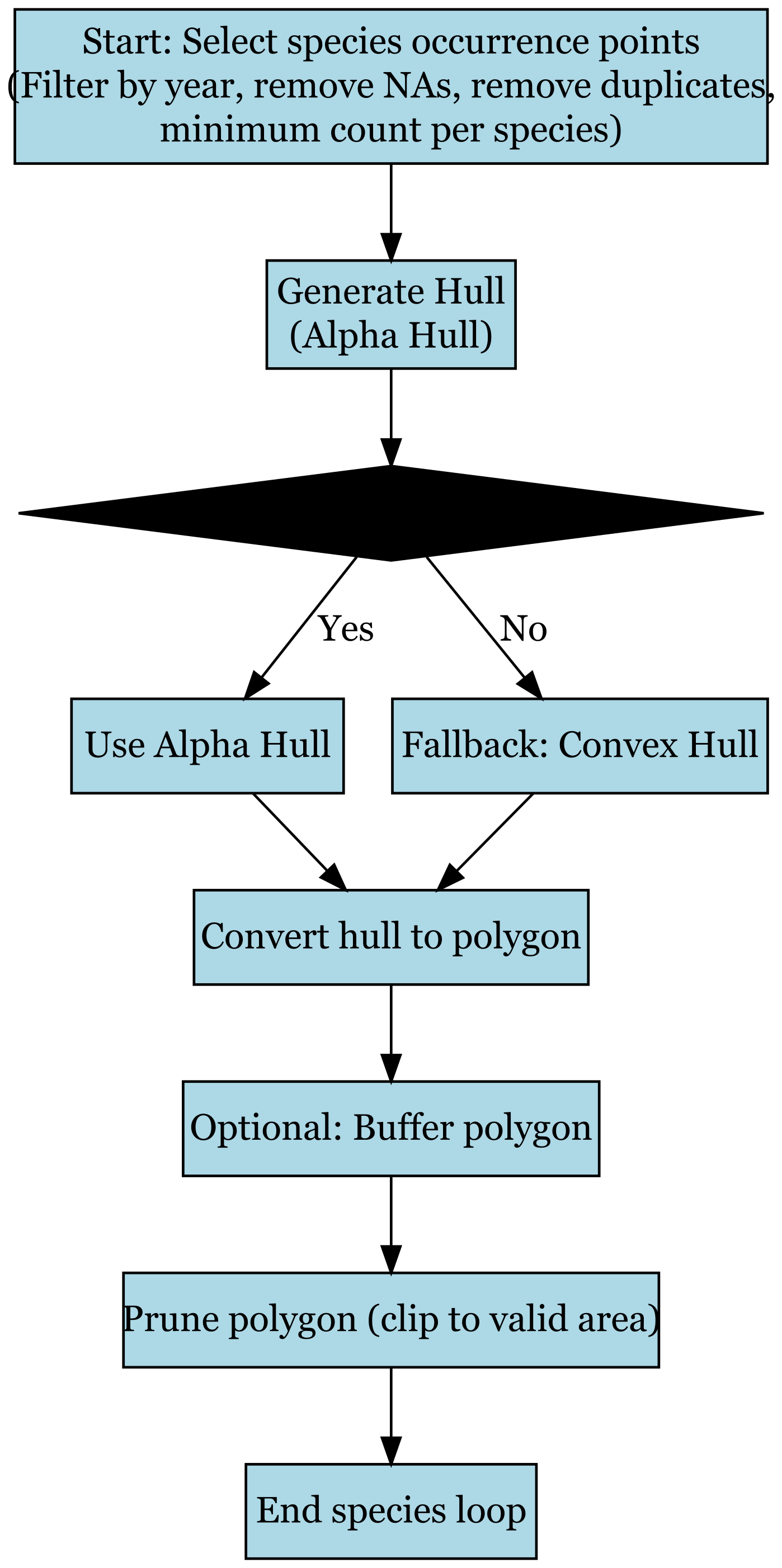
The workflow for species range mapping shown in Fig. B1 begins by selecting species occurrence points, applying a filtering step to remove records with missing coordinates, duplicate entries, or those outside the target time range, while also enforcing a minimum record count per species. After filtering, an alpha hull is generated to approximate each species' distribution. If the alpha hull construction is successful, the result is retained; if not, the procedure falls back to a convex hull. The resulting hull is then converted into a polygon, optionally buffered to smooth edges, and pruned to ensure it aligns with valid geographic boundaries. The process concludes with the finalized range polygon for each species before looping to the next in the dataset.