A framework for gridded estimates of ammonia emissions from agriculture in South Asia

Emissions of ammonia (NH₃) from agricultural activities are a major threat to ecosystems and human health. Its quantification via emissions inventories is vital to the understanding of mitigation strategies and policy formation. South Asia, specifically the South Asian Association for Regional Cooperation (SAARC), is a global hotspot of NH₃ emissions from agriculture but also an area of great uncertainty due to a lack of data that are representative of local practices. This study presents a single implementation of a framework into which indigenous data can be ingested to adjust such estimates, to provide spatially distributed (0.1° × 0.1°) emissions in five agricultural sectors for improved input data for atmospheric chemistry transport models, by moving away from Tier 1 methods for emission inventories (Tomlinson et al., 2025; https://doi.org/10.5285/e0114a4f-32c2-41d9-9c2a-c46f365d4c30). Results incorporate data such as lower emission factors of NH₃ following the application of Urea (13 % of total nitrogen lost as NH₃-N) to provide a total estimated emission of NH₃ in the SAARC of ∼ 6 Tg (±1.2 Tg), with high values (>5 g NH₃ m⁻² a⁻¹) in the Indian states Haryana, Punjab and Uttar Pradesh in the Indo-Gangetic Plain (IGP).

1 Introduction

In South Asia, ammonia (NH₃) pollution from agricultural activities poses significant risks to ecosystems and human health (Sutton et al., 2011; Xu et al., 2018). It is primarily emitted from livestock manures and synthetic fertilizers (e.g. Crippa et al., 2023) and contributes to air and water pollution (Edwards et al., 2024). In ecosystems, elevated NH₃ concentrations and deposition can lead to adverse effects such as soil acidification, nutrient imbalances, and biodiversity loss, particularly in sensitive habitats like forests and wetlands. In humans, NH₃ exposure can cause respiratory issues and exacerbate conditions like asthma. Additionally, NH₃ contributes to the formation of fine particulate matter (PM_2.5), which has severe health implications, including cardiovascular and respiratory diseases (Wyer et al., 2022).

Global emissions inventories, such as the Emissions Database for Global Atmospheric Research (EDGAR) (Crippa et al., 2018; Janssens-Maenhout et al., 2019) and the Hemispheric Transport of Air Pollution mosaic (HTAP) (Crippa et al., 2023), are vital in trying to understand emissions sources and subsequent atmospheric impacts when used as inputs in general circulation climate (GCM) and chemical transport models (CTM) (McDuffie et al., 2020). The former dataset, EDGAR, quantifies emissions with bottom-up calculations which can aid analysis via standardised methods but also by providing global coverage in less data-rich locations, especially when using established products such as the Gridded Livestock of the World (GLW3) (Gilbert et al., 2018) and expert-reviewed methods in the Intergovernmental Panel on Climate Change Guidebook (IPCC, 2006a, 2019). The drawback, however, is a potential omission of country- or region-specific information such as source strength or the underlying spatial distribution of activity data.

In South Asia, agriculture has expanded rapidly, and the increasing use of nitrogen (N) fertilisers has led to a global hot spot of associated gaseous emissions in the region, particularly of NH₃ (Tian et al., 2016; Xu et al., 2018). When assessing mitigation options, relying on aggregated/generalised datasets such as EDGAR may lead to inaccuracies; HTAP, a mosaic approach, attempts to address this issue by incorporating regional inventories, namely the Regional Emission inventory in Asia (REASv3) (Kurokawa and Ohara, 2020) for South Asia, that may represent more spatially specific knowledge.

REASv3 does not exist in isolation; Li et al. (2024) documented MIXv2, a gridded emissions dataset for South and East Asia while Xu et al. (2018) modelled NH₃ emissions across the broader Asia region. Specifically in India, Venkataraman et al. (2018) developed an emissions inventory across multiple source sectors and pollutants while Sahu et al. (2021) inventoried sources of PM_2.5 – however, neither study quantified NH₃ or emissions from agriculture. As such, there is either a paucity of data or a development of interrelated data such as the ingestion of the REASv3 inventory into the MIXv2 model (and also into the HTAP mosaic) and the use of these regional inventories into country specific estimates, such as the use of the REASv2 inventory (Yamaji et al., 2004) to estimate agricultural NH₃ in India (Aneja et al., 2012). However, due to widely acknowledged difficulties in obtaining specific agricultural data, particularly emission factors (EFs) within Asian countries or restricted detailed activity data, many of the top-level datasets such as REASv3 still utilise default methods/EFs outlined in the IPCC (2006a, 2019) or EEA (2019) guidance.

Integrating country-specific data into emissions estimates, and into larger international inventories, can enhance their accuracy and value and foster ownership among participating nations. To do this, it must be clear how new data were included, how emissions estimates have been derived and how aggregated spatial surfaces (which they frequently are) were adjusted when only a part of the underlying data is altered.

In this study, we aim to outline a framework of methods for constructing NH₃ emissions estimates from agriculture, using broadly accepted methodologies but also some country-specific information, to allow a move away from simple, and mostly unrepresentative, Tier 1 methods. We estimate and spatially distribute NH₃ emissions from livestock management, livestock grazing, manure spreading in fields, synthetic fertiliser use, crop residues and agricultural crop waste burning, all at 0.1° × 0.1° resolution. The methodology enables further integration of regional data when available that other compilers can use to improve emissions estimates in their region of interest. We exemplify the methodology in the year 2015 in the South Asian Association for Regional Cooperation (SAARC), which encompasses around 1.7 billion people (2015) in Afghanistan, Bangladesh, Bhutan, India, Maldives, Nepal, Pakistan and Sri Lanka (see Fig. 1). Furthermore, we aim to estimate uncertainty on NH₃ emissions estimates for the five named sectors above, to further complement emissions estimates.

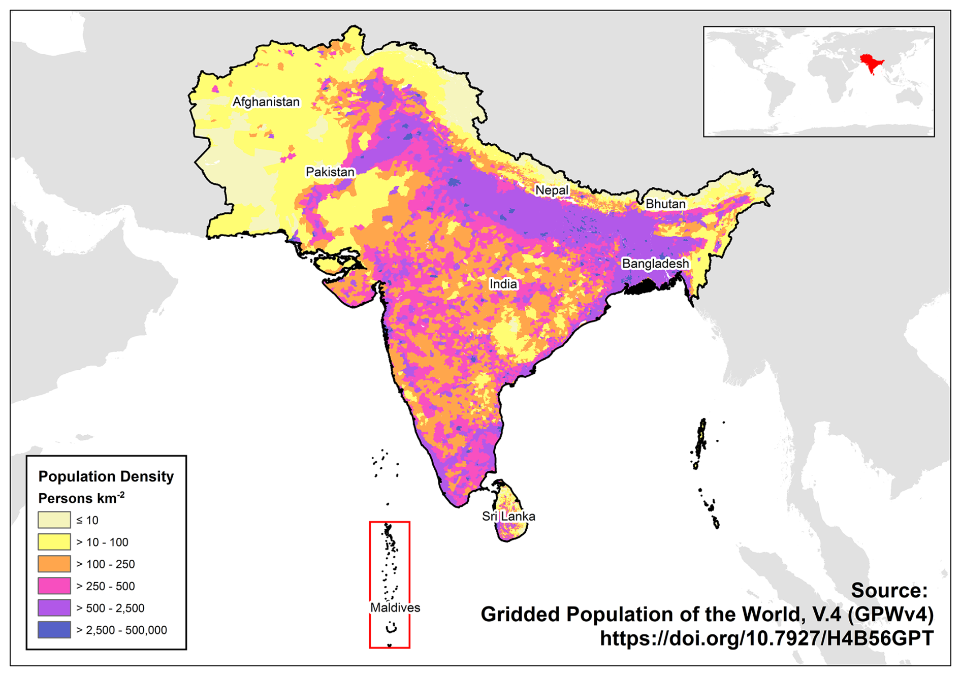
Figure 1 Study area used (black outline), encompassing the eight member countries of the South Asian Association for Regional Cooperation (SAARC), plus population density (persons km⁻²), from the Gridded Population of the World dataset (CIESIN, 2018).

2 Methods

To allow for specific data to be incorporated into regional agricultural NH₃ emissions estimates, we used methods outlined in the EDGARv6.1 methodology (Johansson et al., 2017; Crippa et al., 2018; Janssens-Maenhout et al., 2019), the IPCC 2006 Guidelines (IPCC, 2006a), the IPCC 2019 Guidelines Refinement (IPCC, 2019) and in the EMEP/EEA air pollutant emission inventory guidebooks 2019 (EEA, 2019) and 2023 (EEA, 2023), for estimates of emissions from agricultural soils and livestock management. We applied the same methodology for all eight countries in SAARC, whilst integrating country-specific and/or regional information.

Broadly, total emissions of NH₃ (estimated) from agriculture in the SAARC are surmised by Eq. (1);

$$\begin{array}{}\text{(1)}& E_y={\sum }_{j,k,a}\left[{\mathrm{AD}}_{j,k,a}\cdot {\mathrm{EF}}_{j,k,a}\right]\end{array}$$

where NH₃ emissions (E) in a given year (y) were calculated using the activity data (AD) and NH₃ emission factors (EF), for each sub-sector (k), with a mix of (j) sources, across all areal representations (a). “Areal representation” refers to a spatial unit such as a country, or a state etc. More detail is given in Sect. 2.

Estimates of NH₃ emissions were spatially distributed on a 0.1° × 0.1° grid for five sectors: (i) livestock housing and storage of livestock manures and slurries (livestock management), (ii) spreading of livestock manures and slurries to land and livestock grazing, (iii) synthetic fertiliser application, (iv) crop residues left in fields and (v) agricultural crop residue burning. Emissions from livestock sources were calculated using an N-flow approach (e.g. Webb and Misselbrook, 2004), with N excretion rates calculated head⁻¹ livestock type⁻¹ and N losses estimated separately for housing, storage of manures and slurries, spreading of manures and slurries to land and livestock grazing. Taking this N-flow approach and calculating emission losses at each management stage allowed for finer scale adjustments with country level data and for emission scenarios to be run.

Following estimations of (sub-)sector emission totals, emissions estimates were spatially distributed at a 0.1° × 0.1° resolution, using Eq. (2);

$$\begin{array}{}\text{(2)}& {\mathrm{SE}}_y\left(E,N\right)={\sum }_{p,j,k}\left[E_{j,k}{\displaystyle \frac{p_{j,k}\left(E,N\right)}{\sum _{E,N}\left(p_{j,k,}\left(E,N\right)\cdot H\left(E,N\right)\right)}}\right]\end{array}$$

where spatially distributed emissions (SE) are a function of Easting/Northing coordinates (E, N) distributed by proxy datasets p, where H is the fraction of the grid-cell to the total of T. Further details of sectoral methods and spatial proxies are outlined throughout Sect. 2.

2.1 Synthetic Fertiliser Application

Emissions of NH₃ from the application of synthetic fertilisers (SFA) were estimated using Eq. (3);

$$\begin{array}{}\text{(3)}& \mathrm{E}.{\mathrm{SFA}}_{s,y,a}={\sum }_f\left[{\mathrm{AD}}_{f,a}\cdot {\mathrm{NC}}_{f,a}\cdot {\mathrm{EF}}_{f,\mathrm{ph},a}\cdot {\displaystyle \frac{\mathrm{17}}{\mathrm{14}}}\right]\end{array}$$

Where NH₃ emissions from synthetic fertiliser application (E.SFA) were calculated using AD for a fertiliser type (f), multiplied by its nitrogen content (NC) and the NH₃ emission factor (EF), the latter being dependent on a broad pH class, defined as “normal” or “high” (pH). As EFs are stated as NH₃-N, calculated emissions were multiplied by 17/14 to obtain emissions of NH₃ (molecular weight of N converted to the NH₃ molecule).

For each SAARC member country, national totals of fertiliser used (by type) were taken from FAOSTAT for the year 2015 (Table A1 in the Appendix) (FAO, 2023) and converted into straight N, using fertiliser N content data (Table A2) (FAO, 2023). The FAOSTAT category used was “Agricultural Use”, as this was determined to be a better estimate of actual fertiliser use in that year than “Production”, or “Export”/“Import”. For India, state-wise (sub-national) totals of fertilizer usage (by type) for 2015/16 were compiled from the Indian national statistical database (Indian Agriculture Research Institute (IARI), unpublished data; N. Jain, personal communication, 2022). These data were converted to total N using N content values for each fertilizer type (IARI, unpublished data). Comparisons with FAOSTAT national totals for nitrogenous fertilizer usage showed close alignment, with discrepancies of less than 2 % for total nitrogenous fertilizer and total N applied. The availability of India-specific N content data and sub-national fertilizer usage allowed for an improved spatial distribution of fertiliser application across India than national-level data alone.

To obtain emissions of NH₃, an EF from EEA (2023) (Table A3) was applied to each fertiliser type via a simple lookup schema (Table A4). This EF was spatially influenced by the pH of the topsoil (Batjes et al., 2024), classified to either “normal” (pH ≤ 7) or “high” (pH > 7), as pH is a statistically significant explanatory variable of NH₃ EFs (see EEA, 2023, chap. 3D). In the EEA (2023), Urea fertiliser has an EF of 16 %–17 % of total N lost as NH₃-N (pH dependent); this study used work by Bhatia et al. (2023), drawing upon 20 experimental plots measuring NH₃ emissions from the application of prilled-Urea within South Asia in 2018, to adjust the NH₃ EF of Urea fertiliser to 11.4 % of total N lost as NH₃-N (or 13.8 % as NH₃), which was applied to all SAARC member states. This Urea EF was not measured with pH variability and so was used uniformly in the domain. Whilst this introduces a lack of distinction between higher and lower pH soils, in comparison to non-Urea fertilisers, the initial EF (EEA, 2023) for Urea in high pH soils is only ∼ 5.5 % larger than that in low pH soils, and it was deemed more suitable to use this localised study, even for the loss of pH related sensitivity.

This study used global gridded crop harvest distributions modelled for the year 2000 (EarthStat – Monfreda et al., 2008; Ramankutty et al., 2008; Janssens-Maenhout et al., 2019). All EarthStat crop surfaces were scaled so that the national totals in the SAARC domain matched FAOSTAT reported totals for 2015. For Nepal, state-wise production of 14 principal crops was obtained for 2014/15 (Das et al., 2020) and converted to harvested area using FAOSTAT yield estimates (FAO, 2023). For India, state-wise crop area totals were supplied for 2015/16 (IARI, unpublished data). To ensure consistency between datasets, and to utilise the high spatial resolution of the EarthStat gridded crop area data (0.1° × 0.1°), EarthStat data were scaled to match the Nepal- and India-specific relative state totals, i.e. the proportion of the crop area per state using national statistics, alongside the FAO reported country totals for 2015. This adjustment allowed for a more accurate representation of crop distributions across India and Nepal while maintaining alignment with national data.

This study utilised all 172 crop surfaces available from EarthStat to maximise the amount of cropland represented and combined them with a specific, interpolated (inverse distance weighted), N application per crop by area (Cui et al., 2021). Gridded N application data from Cui et al. (2021) were interpolated to ensure full coverage of N application estimates with all crop areas, although areas of non-intersection were minimal. Table A5 summarises the groups of EarthStat crops matched to the N application rates as modelled in Cui et al. (2021). Where data from Cui et al. (2021) were not used for an EarthStat crop, the overall mean N application rate for that country was used to gap-fill (i.e. national N use/national crop area, in kg N ha⁻¹). Indian state-level crop data were combined with India-specific crop application rates (kg N ha⁻¹) (which superseded Cui et al., 2021, where available), and proportion of crop area fertilised, for a gridded map of total mineral N fertiliser applied (IARI, unpublished data – survey 2011/12).

N application was not modelled by specific fertiliser type and crop due to lack of data (e.g. rate of Urea application to wheat compared to rate of Ammonium Nitrate application to wheat). Individual crop N applications by fertiliser type were aggregated into a single surface and scaled to match the national N application value for that fertiliser as given in FAOSTAT (FAO, 2023) (IARI, unpublished data, for India). This aggregated N application, determined by crop distributions along with the pH data, was used as the proxy to distribute estimated NH₃ emissions for mineral fertiliser (Eqs. 2 and 3).

2.2 Crop Residues

Emissions of NH₃ (estimated) from crop residues remaining in the field (CRR) are outlined in the EMEP/EEA guidebook 2023 (EEA, 2023) with further details from the IPCC 2019 Guidelines Refinement (IPCC, 2019). Emissions were estimated for above ground residues only, as below ground crop residues are not relevant for NH₃ emissions. Emissions of NH₃ from crop residues are highly uncertain as the underlying assumptions are not well understood. Essentially, emissions were estimated from above ground biomass that is not removed, incorporated or burnt, via Eq. (4);

$$\begin{array}{}\text{(4)}& \mathrm{E}.{\mathrm{CRR}}_y={\sum }_c\left[{\mathrm{HA}}_c\cdot \left({\mathrm{AGDM}}_c\cdot {\mathrm{NAG}}_c\right)\cdot {\mathrm{FF}}_c\cdot {\mathrm{EF}}_c\right]\end{array}$$

Where NH₃ emissions from crop residues (E.CRR) for a crop type (c) were calculated using the total harvested area (HA) taken from FAOSTAT (FAO, 2023), the above ground dry matter fraction (AGDM – a linear equation using yield and dry-matter) (IPCC, 2019), the N content of above-ground residues (NAG) and the fraction of the crop residues that remain on the field (FF), following subtraction of removals (FR), incorporation (FI) and burning (FB) – see details in Sect. 2.3 for crop residue burning. Crop residue removals, FR, are residues that might be used for fodder, domestic fuel and building materials and can vary from crop to crop and area to area. FI was set to 0 in this study due to a lack of data. Additionally, AGDM was calculated using the crop yield (FAOSTAT, FAO, 2023), the crop dry matter (DM_c) content and information on the ratios of remaining biomass to pre-harvested crop (Table 11.2, Chap. 11, IPCC, 2019) – Table A6 outlines crop parameters used for crop residue (and burning) emissions, and notes the changes made to DM content and FR with particular reference to the SAARC domain (Gadde et al., 2009; Jain et al., 2014; Azhar et al., 2019; Das et al., 2020).

For each SAARC member state, total harvested areas of crops were taken from FAOSTAT for the year 2015 (FAO, 2023). There are limited studies that have researched NH₃ EFs for crop residues and so the model of de Ruijter and Huijsmans (2019), in EEA (2023), was used via Eq. (5), to place into Eq. (4) (EF in g NH₃ kg⁻¹ DM);

$$\begin{array}{}\text{(5)}& \mathrm{EF}\left(\mathrm{CRR}\right)=\left\{\begin{array}{ll}\mathrm{0}& \mathrm{NAG}\le \mathrm{0.0132}\\ \frac{\mathrm{410}\cdot \mathrm{NAG}-\mathrm{5.42}}{\mathrm{100}}& \mathrm{NAG}>\mathrm{0.0132}\end{array}\right.\end{array}$$

NH₃ emissions were distributed onto the re-weighted EarthStat crop surfaces by country and crop (see Sect. 2.1), using the relative weight of the harvested area as the proxy for estimated NH₃ emissions.

2.3 Agricultural Waste Burning

Emissions of NH₃ (estimated) from agricultural crop residues burnt (above ground only) (CRB) are outlined in the EMEP/EEA guidebook 2023 (EEA, 2023) and the IPCC 2019 Guidelines Refinement (IPCC, 2019). The fraction of crop residues that are burnt in the field, FB, is intrinsically linked with crop residue estimations via FF in Eq. (4), that is FB = $\mathrm{1}-\mathrm{FR}-\mathrm{FF}-\mathrm{FI}$. NH₃ emissions were obtained via Eq. (6);

$$\begin{array}{}\text{(6)}& \mathrm{E}.{\mathrm{CRB}}_y={\sum }_c\left[{\mathrm{HA}}_{c,y}\cdot {\mathrm{AGDM}}_c\left({\mathrm{FB}}_c\cdot {\mathrm{Cf}}_c\right)\cdot {\mathrm{EF}}_c\right]\end{array}$$

Where NH₃ emissions from crop residues burnt (E.CRB) for a crop type (c) were calculated using the FB of DM, a combustion completeness factor (unitless, Cf) and an EF (g NH₃ kg⁻¹ DM). For all countries aside from India, the FB for crop type (c) was restricted to: barley, beans (dry), groundnuts, jute, lentils (dry), maize, millet, potatoes, rape/colza, rice, sugar cane and wheat (Kumar and Singh, 2021; Lin and Begho, 2022) (FAOSTAT naming convention). For India, specifically, the crop type (c) was restricted to: maize, rice, sugar cane and wheat (Jain et al., 2014; N. Jain, personal communication, 2024), as these are the crop residues predominantly burnt in fields in South Asia and India respectively.

As agricultural crop residue burning is common practice in South Asia (Azhar et al., 2019), attempts to improve the quality of EFs and their spatial distribution are supplemented with regional information, summarised in Table A6. The standard value of FB used was 0.233, as derived from Yevich and Logan (2003), and was supplemented with other information when known, along with Cf (Table A6) (Haider, 2013; Jain et al., 2014; Azhar et al., 2019; Das et al., 2020; Somarathne and Lokupitiya, 2024). Any crop not in the sets defined above was specified as FB = 0. Table 1 shows the values for FB used crop⁻¹ country⁻¹.

Table 1 Values used for the fraction of crop residues left in the field that are burnt (FB). One value of 0.233 is used for all crops considered in all countries and updated where national data are found (updated values are bold).

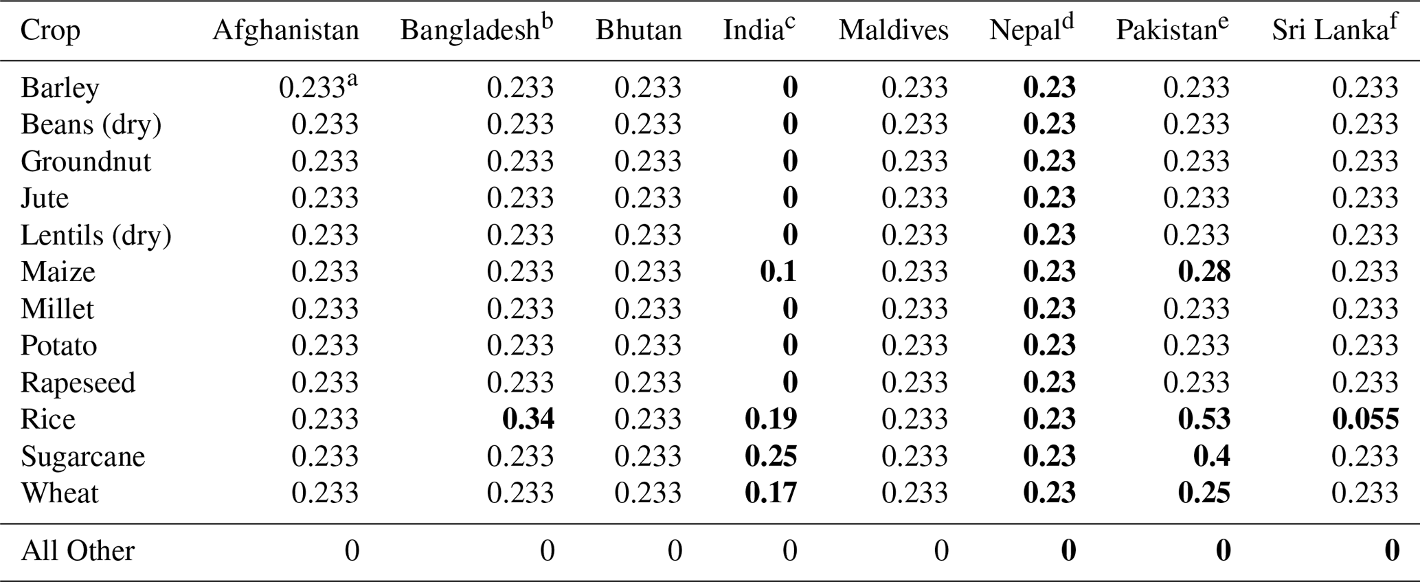
^a All values of 0.233 are from Yevich and Logan (2003). ^b Haider (2013). ^c Jain et al. (2014). ^d Das et al. (2020). ^e Azhar et al. (2019). ^f Somarathne and Lokupitiya (2024).

EFs of NH₃ are difficult to measure for burnt crop residues, and many regional studies reference, directly or indirectly, key studies such as Dennis et al. (2002), Li et al. (2007) and Andreae and Merlet (2001). Due to the range of NH₃ EFs across crops, and the uncertainty, a mean NH₃ EF across all crops was taken. Measuring Cf for crop residue burning is difficult, therefore researchers have proposed the use of modified combustion efficiency (MCE) (e.g. Yokelson et al., 2011; Stockwell et al., 2015). MCE is the ratio $\mathrm{1}{\mathrm{CO}}_{\mathrm{2}}/(\mathrm{1}{\mathrm{CO}}_{\mathrm{2}}+\mathrm{1}\mathrm{CO})$ (Yokelson et al., 1996); high MCE (∼ 0.99) represents more complete oxidation, while a lower MCE (∼ 0.75–0.84 for biomass fuels) represents pure smouldering (Stockwell et al., 2016). The EF in the present study for crop residues burnt is 1.57 g NH₃ kg⁻¹ DM (SD = 1.17), a mean of six MCE values across rice, wheat, maize and generic crops, plus the US-EPA NH₃ EF (Lee and Atkins, 1994; Dennis et al., 2002; Christian et al., 2003; Li et al., 2007; Yokelson et al., 2011; Stockwell et al., 2015; Stockwell et al., 2016). This EF was applied to each crop type (c) but could simply be replaced with better data, at the crop level, when obtained.

NH₃ emissions were distributed onto the reweighted EarthStat crop surfaces by country and crop (see Sect. 2.1), using the relative weight of the harvested area as the proxy for estimated NH₃ emissions.

2.4 Livestock

Emissions of NH₃ from livestock were estimated using a N flow approach, with losses estimated during housing, storage of manures and slurries, spreading of livestock manures and slurries to land and livestock grazing, and are laid out in the following sub-sections. The N flow approach starts with N excretion by livestock and then follows the flow of N through the manure management chain (and also estimates losses for unmanaged livestock). N excretion rates were calculated via Eq. (7);

$$\begin{array}{}\text{(7)}& {\mathrm{Nx}}_{t,y}={\mathrm{Nxm}}_{t,y}.\left({\mathrm{TAM}}_t.{\mathrm{AAP}}_{t,y}\right)\end{array}$$

Where the total N excretion (Nx; kg yr⁻¹) for each livestock type (t, as detailed in Table A7) per annum (y) was calculated by multiplying Annual Average Population (AAP; FAOSTAT) by the Typical Animal Mass (TAM, FAO, 2024) and applying a N excretion rate by mass (Nxm; kg N kg animal mass⁻¹ yr⁻¹, FAO, 2024). The total N excreted (Eq. 7) is then separated into the proportion deposited within buildings or uncovered during grazing. These proportions depend on the fraction of the year that animals spend in buildings, on yards and grazing, and on animal behaviour. Statistics on the fraction of excreta that was managed, and the type of store used was taken from FAO (2024). Grazing emissions were estimated from the unmanaged fraction (excreta on pasture or used for fuel) and housing, storage and spreading emissions were calculated for managed manures (i.e. solid and slurry systems).

Emissions of NH₃ (estimated) from livestock grazing (GRA) are emissions from N in excreta that are not associated with any manure management systems (i.e. not excreted during the housing period and/or subsequently stored and spread). The total amount of N excreta, which are applicable to grazing emissions are estimated in Eq. (8);

$$\begin{array}{}\text{(8)}& \mathrm{Nx}.{\mathrm{grz}}_{t,y}=\left({\displaystyle \frac{{\mathrm{Nx}}_{t,y}\cdot \mathrm{F}.{\mathrm{fuel}}_t}{\mathrm{2}}}\right)+\left({\mathrm{Nx}}_{t,y}\cdot \mathrm{F}.{\mathrm{pasture}}_t\right)\end{array}$$

Where the amount of N excreta that is subject to grazing emissions (Nxgrz) by livestock type (t), i.e. on pasture, range and paddocks, is calculated by multiplying Nx_t by the fraction going to pasture (FAO, 2024) and by summing half of the N excreted that is burned for fuel to account for the N excreted in the urine. NH₃ emissions from grazing were then estimated via Eq. (9);

$$\begin{array}{}\text{(9)}& \mathrm{E}.{\mathrm{grz}}_{t,y}=(\mathrm{F}.{\mathrm{TAN}}_t\cdot \mathrm{Nx}.{\mathrm{grz}}_{t,y})\cdot \mathrm{EF}.{\mathrm{grz}}_t\end{array}$$

Where grazing emissions (Egrz) per livestock type (t) were calculated by estimating the TAN content of N excreta subject to grazing emissions (Nxgrz) and applying the EF for grazing (EF.grz_t, EEA, 2023).

Emissions of NH₃ from housing were calculated for the proportion of excreta on managed systems. The amount of N excreta on managed manure systems and subject to housing emissions (Nx.h_t) is given by subtracting the total N excreta on pastures (Nx.grz_t, Eq. 8) from total N excreta (Nx_t, Eq. 7). Housing emissions are then estimated via Eq. (10).

$$\begin{array}{}\text{(10)}& \mathrm{E}.{\mathrm{h}}_{t,y}=\sum _s\left[\mathrm{Nx}.{\mathrm{h}}_{t,s,y}\cdot \mathrm{F}.{\mathrm{TAN}}_{t,s}\cdot \mathrm{EF}.{\mathrm{h}}_{t,s}\right]\end{array}$$

Where emissions from livestock housing (E.h) by livestock type (t) is calculated as the sum of emission estimates by manure system (s; i.e. separate estimates from slurry and solid manures). Housing emissions are estimated by multiplying the N excretion at the housing stage (Nx.h) by the fraction of TAN (F.TAN_t,s) and by housing emission factor (EF.h_t,s, EEA, 2023).

Storage emissions are then estimated via Eq. (11) and are based on the amount of TAN remaining after housing losses. The amount of TAN entering storage systems (TAN.str) by livestock type and manure system is calculated by subtracting housing losses (E.h) and excreta on daily spread systems (which are not stored for any substantial period of time) from N excreta entering housing (i.e., TAN.h_t,s = Nx.h_t,s ⋅ F.TAN_t,s).

$$\begin{array}{}\text{(11)}& \mathrm{E}.{\mathrm{str}}_{t,y}=\sum _s\left[\mathrm{TAN}.{\mathrm{str}}_{t,s,y}\cdot \mathrm{EF}.{\mathrm{str}}_{t,s}\right]\end{array}$$

Where emissions from storage (Estr) by livestock type (t) is calculated as the sum of emission estimates by manure system (s; i.e. separate estimates from slurry and solid manures). Storage emissions are estimated by multiplying the TAN entering the storage stage (TANstr) by the storage emission factor (EF.str_t,s, EEA, 2023) by livestock type (t) and manure system (s).

To calculate the amount of TAN from livestock manures/slurries applied to land, N losses to the atmosphere (as N₂O and N₂) need to be subtracted from TAN entering housing (TAN.h), in addition to subtracting ammonia emissions from housing and storage. Emission estimates of N₂O (E.N₂O) and N₂ (E.N₂) were estimated using default values from Misselbrook et al. (2015) and used to estimate TAN entering spreading stage (TAN.spr) as expressed in Eq. (12);

$$\begin{array}{}\text{(12)}& \begin{array}{rl}\mathrm{TAN}.{\mathrm{spr}}_{t,s,y}& =\mathrm{TAN}.{\mathrm{h}}_{t,s,y}\\ & -{\left[\mathrm{E}.{\mathrm{N}}_{\mathrm{2}}\mathrm{O}+\mathrm{E}.{\mathrm{N}}_{\mathrm{2}}+\mathrm{E}.\mathrm{h}+\mathrm{E}.\mathrm{str}\right]}_{t,s,y}\end{array}\end{array}$$

Where the amount of TAN entering the spreading stage (TAN.spr_t,s) is assumed to be TAN entering housing (TAN.h) minus the sum of all N losses from housing and storage. TAN entering housing is used as the starting point as TAN on daily spread systems also needs to be included in the TAN being spread.

NH₃ emissions from manures and slurries applied to land are calculated via Eq. (13);

$$\begin{array}{}\text{(13)}& \mathrm{E}.{\mathrm{spr}}_{t,y}=\sum _s\left[\mathrm{TAN}.{\mathrm{spr}}_{t,s,y}\cdot \mathrm{EF}.{\mathrm{spr}}_{t,s}\right]\end{array}$$

Where emissions from spreading (Espr) by livestock type (t) is calculated as the sum of emission estimates by manure system (s; i.e. separate estimates from slurry and solid manures). Spreading emissions are estimated by multiplying the TAN entering the spreading stage (TANspr) by the spreading emission factor (EF.spr_t,s, EEA, 2023) by livestock type (t) and manure system (s).

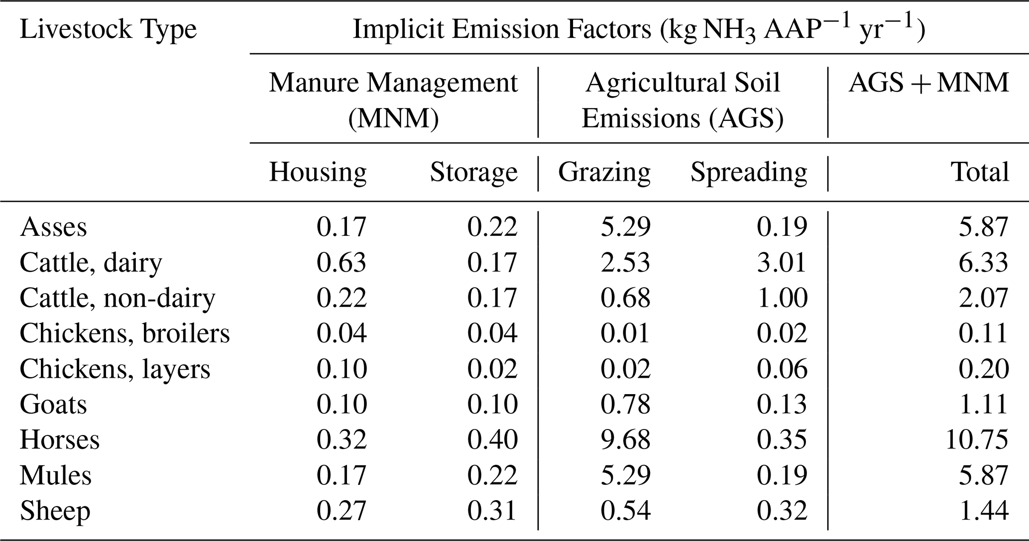
Implicit EFs from the livestock emission calculations (Eqs. 8, 9, 10 and 12) are presented in Table A8 and were estimated by dividing emissions at each stage by AAP. Country level emission totals (per livestock type) were aggregated to the most appropriate dasymetric Gridded Livestock of the World v4 livestock category (GLW v4 – Gilbert et al., 2018) (see Table A7). Emissions were spatially distributed to the 0.1° × 0.1° GLWv4 livestock distributions using the cell-level proportions of national livestock totals. From Sect. 3 onwards, emissions from the above N-flow that are from grazing and manure spreading activities will be referred to as GRM and those from livestock management activities as MNM.

2.5 Uncertainty

To estimate uncertainty in NH₃ emissions, multiple quantitative uncertainty estimates were combined using Monte Carlo–based error propagation. Uncertainty propagation distinguished between within-country and cross-country dependence. Sub-sectoral emissions within each country were treated as correlated, reflecting shared underlying drivers such as crop parameters, national statistics (e.g. total N usage, total crop area), livestock numbers and TAM. In contrast, country totals were aggregated assuming independence, reflecting largely country-specific activity data. As a result, the regional uncertainty is smaller than the sum of individual country uncertainties.

Uncertainty arises from many sources, including the activity data (e.g. statistical error, data collection bias and extrapolation) and the emission factors (e.g. experimental uncertainty, representativeness and random error). Table 2 summarizes the uncertainty values that have been used in this study for the purposes of uncertainty estimation. The IPCC commonly reports uncertainty as a percentage corresponding to two standard deviations, e.g. ±15 %, approximating a 95 % confidence interval around a best estimate, under an assumption of normality in the underlying data (IPCC, 2006b, d). Other sources (e.g. Tang et al., 2024) provide “indicative” uncertainty ranges; in these cases, the implied or reported coefficient of variation (CV; standard deviation divided by the mean) was applied alongside the best estimate for the same uncertainty source. Where available, uncertainties were derived directly from reported standard deviations around a mean. All uncertainties in Table 2 are expressed as CV values.

Table 2 Sources of uncertainty used in this study, all converted to a coefficient of variation for consistency and comparability. A range of values indicates country specific CV values, or livestock types. EF =  emission factor.

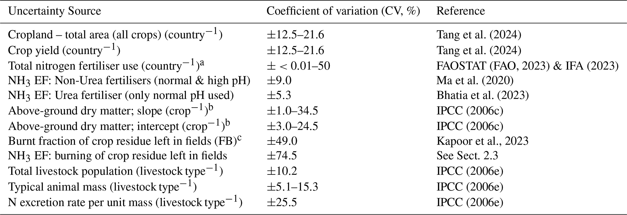
^a Uncertainty for fertiliser application rates (kg N ha⁻¹) were derived from total estimated crop area and total N applied per country within the Monte Carlo propagation, and applied uniformly to each crop application rate from Cui et al. (2021). ^b IPCC (2006c) lists slope and intercept values for a linear equation to derive AGDM, along with uncertainty, for crops stated in Table A6. ^c Uncertainty for FB was taken from Kapoor et al. (2023), who quoted six studies of total burnt residue area in South Asia. We use the SD and mean from those six studies to derive a CV of 49 % for all crop FB values.

3 Results

Total emissions of NH₃ were estimated to be 6025 kt NH₃ a⁻¹, for 2015, in the SAARC study area, with an uncertainty of ±1179 kt NH₃ a⁻¹ (95 % confidence interval). Table 3 shows a sectoral breakdown of these emissions, for each SAARC member country, while Fig. 2 shows the spatial distributions of sectoral emissions across the area for 2015.

Table 3 Estimated emissions of NH₃ country⁻¹ sector⁻¹ a⁻¹, for 2015, in kt NH₃. 0 = an emission less than 0.05 kt NH₃ but more than zero. “–” = zero. CRB = Agricultural crop residue burning, CRR = Crop residues left in fields, GRM = Livestock grazing & manure spreading, MNM = Livestock management, SFA = Synthetic fertiliser application.

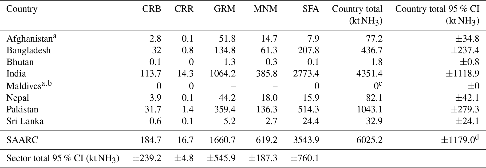
^a There were no Agricultural Use statistics for fertiliser products, only total Nitrogen usage. Emissions were calculated using the Tier-1 EF provided by EEA (2023) (see Table A3) (derived via a mixture of Tier-1 and Tier-2 methods). ^b There were no livestock statistics in the FAOSTAT database for the Maldives. ^c Estimated total NH₃ emissions for Maldives = 0.02 kt NH₃ a⁻¹. ^d Regional uncertainty reflects aggregation of country totals assuming independence across countries; it is therefore not equal to the sum of national confidence intervals

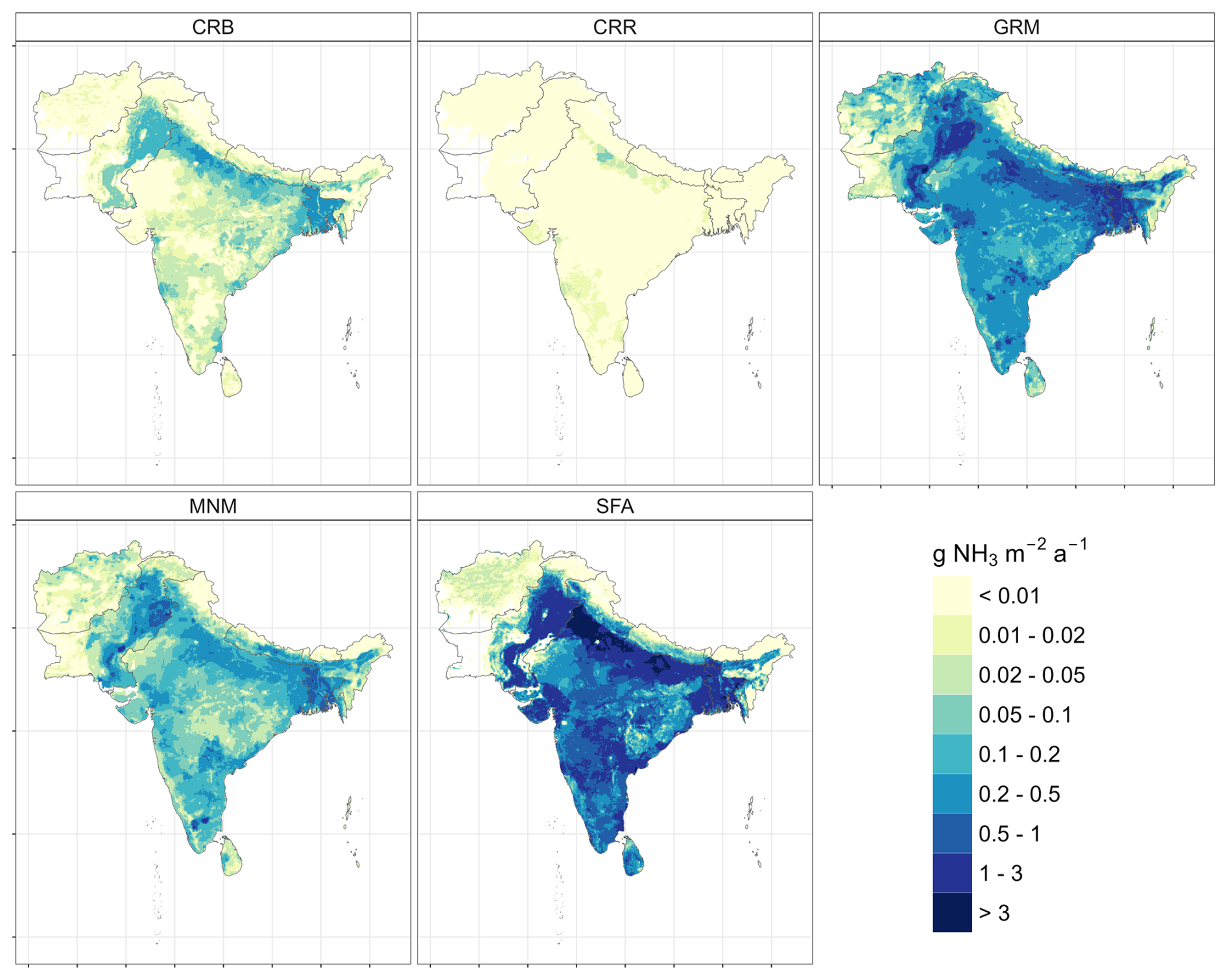
Figure 2 Emissions of NH₃ (g m⁻² a⁻¹) in five agricultural sectors, spatially distributed on a 0.1° × 0.1° resolution (common scale/legend): Agricultural crop residue burning (CRB), crop residues left in fields (CRR), livestock grazing & manure spreading (GRM), livestock management (MNM) and synthetic fertiliser application (SFA).

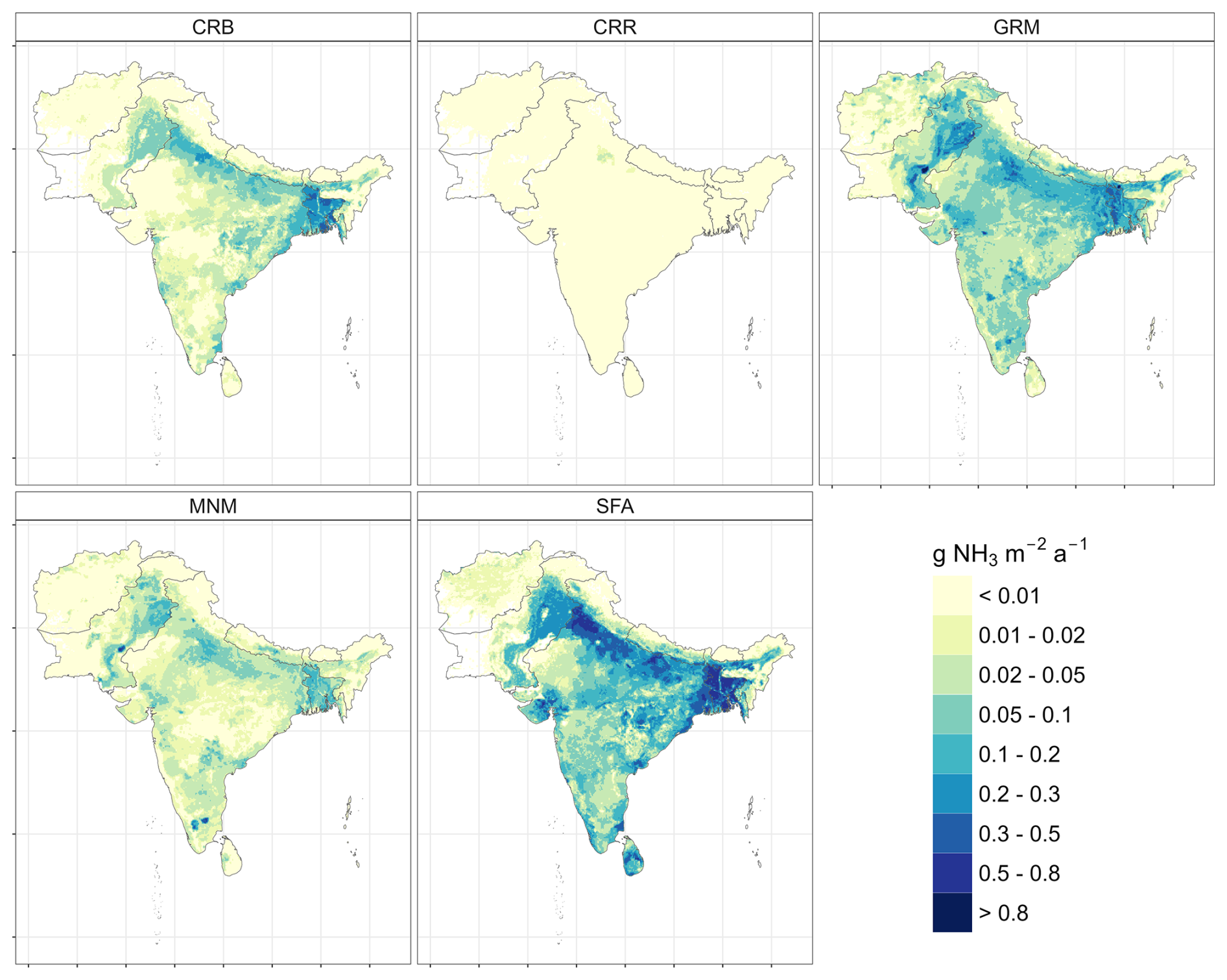
Figure 3 Uncertainty (standard deviation) of emissions of NH₃ (g m⁻² a⁻¹) in five agricultural sectors, spatially distributed on a 0.1° × 0.1° resolution (common scale/legend): Agricultural crop residue burning (CRB), crop residues left in fields (CRR), livestock grazing & manure spreading (GRM), livestock management (MNM) and synthetic fertiliser application (SFA).

Figure 3 shows the estimated uncertainty (as standard deviation) for the same sectoral spatial distributions. Emissions from SFA were the largest contributor to the regional total (59 % of SAARC total, range 7 % to 74 % at the country level), despite a reduction in the EF for Urea use, compared with the EEA (2023) value, in the present study (see Sect. 2.1), followed by GRM. Spatially, the Indo-Gangetic Plain (IGP) was a key source of NH₃ emissions in the SAARC, particularly in the Indian states of Haryana and Punjab due to the high quantities of synthetic N fertilisers applied, but also the western districts of Bangladesh. Higher emissions from GRM were located in the west of the IGP on the Rajasthan Plain and in Bangladesh, due to large numbers of cattle and buffaloes (see Fig. 2). Similarly, high emissions from GRM were located in Pakistan due to large numbers of Buffalo in the underlying GLW population surfaces. Uncertainty within India represents the largest emissions values grid cell⁻¹, especially for SFA, but the relative sectoral uncertainty (CV) is highest in CRB (range 45 % to 90 % at the country level), due to the highly uncertain EF and also the uncertainty in burnt area.

Overall, 91 % of the total harvested crop area reported in 2015 (FAOSTAT, FAO, 2023) was estimated via 172 EarthStat layers (each crop layer was then scaled to match the reported FAO harvested total), and, subsequently, ∼ 103 % of total N use from synthetic fertiliser reported in 2015 (FAOSTAT, FAO, 2023) was estimated using a mix of bottom-up crop-specific fertiliser application rates (see Table A5), plus generic application rates derived from country total crop area and total fertiliser application. This lends some confidence to the distribution of N fertiliser using crop statistics. Total N fertiliser usage was then re-scaled to match the FAOSTAT national totals at 100 % (using an uncertainty derived from FAOSTAT and IFA, in Table 2). There was a general underestimation in the harvested area of rice (all countries) and wheat (India and Pakistan) in EarthStat data compared to FAO totals, and an over estimation of total N application in Bangladesh, Nepal and Sri Lanka prior to adjustment to FAO totals. The reason for an underestimation of harvested rice area specifically is not known, as only Pakistan has undergone any reasonable expansion in rice production since 2000, but may be due to the difficulty of estimating areas of paddy rice due to an increased number of growing seasons per year.

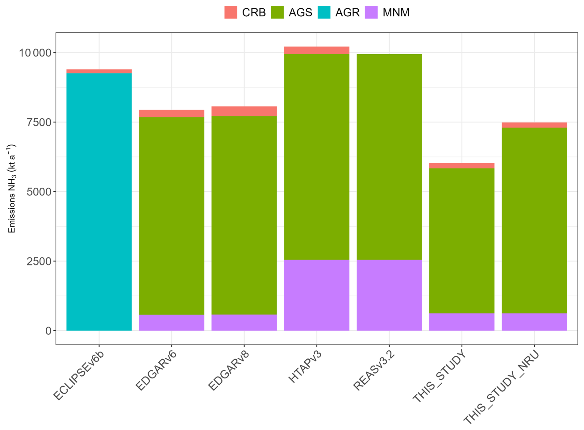
Figure 4 Total agricultural NH₃ emissions (kt a⁻¹): this study (THIS_STUDY), this study when recalculated with non-reduced EEA (2023) EF values for Urea fertiliser (i.e. a higher EF) (THIS_STUDY_NRU), four global inventories (ECLIPSEv6b, HTAPv3 and the two most recent versions of EDGAR – v6 and v8) and one regional inventory (REASv3.2). Emission sectors are agricultural soils (AGS), crop residue burning (CRB), general agriculture (AGR) and manure management (MNM).

Figure 4 compares agricultural NH₃ emissions from several regional/global inventories with the present study. Due to the aggregation of agricultural emissions in other inventories, the totals of some of the finer-resolution categories in this study were aggregated to agricultural soils (SFA + GRM + CRR = AGS), with manure management (MNM = MNM) and agricultural crop residue burning (CRB = CRB) at their original category resolution. The ECLIPSE inventory does not provide separated estimates for agricultural soils and manure management estimates, but only total agriculture (AGR = AGS + MNM) and CRB, while REAS does not provide estimates for CRB. Also displayed is the total derived in the present study when using a non-lowered EF for Urea fertiliser application from EEA (2023) (labelled THIS_STUDY_NRU).

Prior to the inclusion of a lower EF for Urea fertiliser, total emissions of NH₃ from agricultural sources in this study were 7486 kt; 6 % and 7 % lower than those estimated in the EDGARv6 and v8 databases respectively, 20 % lower than ECLIPSE and 27 % lower than HTAP. Adjusting the Urea EF (to 13 % of total N lost as NH₃-N, see Sect. 2.1, and referred to as THIS_STUDY_NRU in Fig. 4) reduced total emissions by a further 20 %. At the country level (following the Urea EF reduction), NH₃ emissions in Bangladesh, Pakistan and India were ∼ 17 %, ∼ 17 % and ∼ 28 % lower than those calculated by EDGARv8, respectively, and ∼ 35 %, ∼ 24 % and ∼ 43 % lower than emissions estimated in HTAPv3, respectively. Figure 5 shows a comparison of the spatial distributions of total estimated NH₃ from agriculture for multiple inventories (totals shown in Fig. 4). (N.B. there are no livestock numbers in FAOSTAT for the Maldives, while EarthStat crop maps do not have data for the Maldives, resulting in no spatially distributed emissions.)

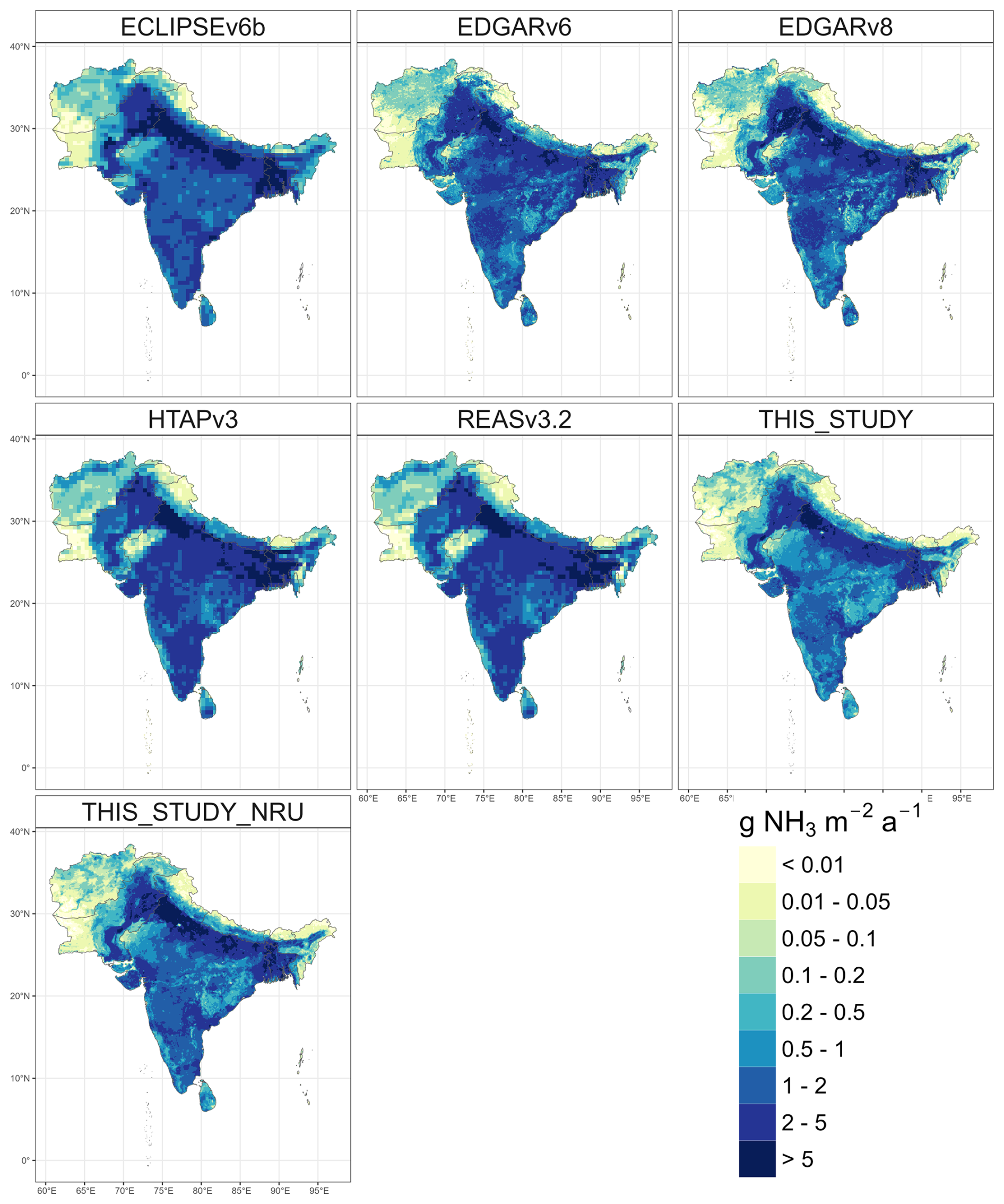
Figure 5 Total emissions of NH₃ (g m⁻² a⁻¹) in 2015 from agriculture from seven datasets, spatially distributed on varying resolutions (in brackets): ECLIPSEv6b (0.5° × 0.5°), EDGARv6 (0.1° × 0.1°), EDGARv8 (0.1° × 0.1°), HTAPv3 (nominally 0.1° × 0.1°), REASv3.2 (0.25° × 0.25°), this study (THIS_STUDY) (0.1° × 0.1°) and this study when recalculated with non-reduced EEA (2023) EF values for Urea fertiliser (i.e. a higher EF) (THIS_STUDY_NRU) (0.1° × 0.1°).

4 Discussion

NH₃ emissions estimates in this study were ∼ 25 % lower than the most recently published EDGAR dataset (EDGARv8) and ∼ 40 % lower than the HTAPv3 global mosaic. A major driver of this difference was the use of an EF for Urea fertiliser application that was 19 % to 23 % lower than the EEA (2023) default value (pH dependent) (see Sect. 2.1) and 38 % lower than the EF in Bouwman et al. (2002), the latter being used in EDGARv6 (Crippa et al., 2018; Janssens-Maenhout et al., 2019). As Urea constituted 82 % of applied synthetic N and 84 % of fertiliser application emissions, which were, in turn, responsible for 59 % of agricultural emissions (in this study), any decrease/increase in EF had a pronounced effect. Sub-national (state) level statistics for crop harvest areas in Nepal and both fertiliser use and crop harvest areas in India allowed for greater spatial representation of the use of fertilisers (but not for specific fertiliser use on specific crops). In India there was a decrease in emissions from fertilisers in central Andhra Pradesh and coastal Tamil Nadu, and a simultaneous increase in Punjab and Haryana, while in Nepal emissions have been concentrated more in the eastern half of the country compared to national fertiliser use statistics and non-adjusted crop maps. This study used 172 crop distributions from EarthStat, compared to 24 crops in EDGARv6, and gridded N application rates per crop from Cui et al. (2021).

Emissions of NH₃ from CRB were estimated at 185 kt a⁻¹, roughly half of that estimated in EDGARv8 and a third lower than HTAPv3. This study used only a specific subset of crops for burnt area estimates following a literature review, but it is clear that more data are required. Due to the importance of crop residue burning to ambient fine particulate matter (PM_2.5) formation, particularly in proximity to urban areas (e.g. Lan et al., 2022), more information is needed within the SAARC domain on the crops that undergo burning, the proportion of the crop burnt and the spatial variability of burning practice. The portion of crop residue left on fields for burning after harvesting the crop using combines/machinery, and location-specific other usage of crop residues, should also be taken into account. Mechanical harvesters leave more residue that is subsequently burnt and so a mechanization ratio can be used to adjust the amount of stubble/straw left in the fields (e.g. Li et al., 2007). This could be incorporated via survey work for better estimates of emissions from residue burning (Azhar et al., 2019) but would require consideration of the representativeness of such a survey for a large heterogeneous region. The amount of residue burnt has a direct impact on, and is directly impacted by, the quantity of residues left in-field (see Eq. 4), and therefore more detailed information is required as to the use of crop residues for domestic fuels or livestock fodder to make better estimates of emissions from CRR. Furthermore, the EFs for residues burnt and (Sect. 2.2) residues left in-field (Sect. 2.3) remain highly uncertain and, despite the availability of measurement data on varying crop types, it was decided that only one EF per sector for generic “crop” was suitable for use at this time. While NH₃ emissions appear to be small for CRB and CRR combined (3.5 % of total agricultural NH₃ in this study), the uncertainty around this source is large and better understanding will also aid other sectors such as MNM, domestic burning (and emissions of other pollutants).

With regards to emissions from livestock, there is a good agreement in regional NH₃ totals between this study and the EDGAR releases (including the grazing and spreading emissions), but a large disparity between this study and the REAS/HTAP estimates, particularly with the manure management stage. As far as can be ascertained, all studies evaluated emissions from housing, storage, yards, grazing and spreading of manures/slurries with regards to livestock, but applied different methods. This study used an N flow approach outlined in Sect. 2.4, drawing upon IPCC (2019) and EEA (2023), while REAS/HTAP used Tier 1 EFs as provided in the EMEP EEA Guidebook 2016 (this guidebook is unavailable, further reference to Tier 1 EFs are in EEA 2019). As an example, this study has an overall Tier 1 EF (sum of grazing, manure management and spreading emissions) of 6.33 kg NH₃ per head per annum for dairy cattle, compared to 41.8 kg NH₃ (slurry systems) and 26.4 kg NH₃ per head (solid systems) in the EEA (2019) (N.B. the EEA Guidebook provides EFs for annually averaged population, AAP, which we assume to be 1 for dairy cattle). It is unclear how Tier 1 EFs for slurry and solid systems (EEA, 2019) were utilised in REASv3.2 (which is used as a direct input in the HTAP mosaic). The difference can, in part, be explained by the underlying assumption of Typical Animal Mass (TAM) in the calculation of estimated total N excretion by animal type (Nx, Eq. 7, Sect. 2.4). In this study, dairy cattle were assumed to have a TAM of 275 kg head⁻¹ across the study region (FAO, 2024), compared to the underlying assumption of EEA (2019) Tier 1 EFs that assume a TAM of 600 kg head⁻¹, corresponding to intensively reared dairy cattle typical in western nations. This 118 % increase in TAM directly impacts the sectoral N excretion. Furthermore, a large proportion of N excreta in the study region (55 %) is collected, dried and used as fuel (FAOSTAT, FAO, 2023). In western nations, the burning of these “dung cakes” is uncommon and most N excreta are on managed systems and applied to fields as organic fertiliser. Emissions associated with the burning of dung cakes is reported under residential combustion, rather than agriculture and therefore the T1 emissions are likely an overestimation for South Asia. This disparity between estimates in this paper and a T1 approach highlights the importance of considering spatially disaggregated information on TAM and livestock management systems to produce more accurate NH₃ emissions estimates, and methods that allow for the incorporation of regionally relevant data. While this study has used country level estimates of TAM and N excretion rates (Nxm) from FAO, these estimates are currently the same for each country within SAARC and consequently the implicit EFs derived under this study are the same for each country (Table A8). Furthermore, REASv3.2 uses animal distributions that are land cover-based distributions of sub-national livestock statistics from REASv1 (Yamaji et al., 2004), as opposed to this study and other inventories (e.g. EDGAR) which have used GLW livestock distributions. This issue highlights the difficulty in using T1 EFs and how hard they can be to adapt to different regions of the world.

Estimated uncertainty in total NH₃ emissions from agriculture was estimated and may originate from AD (e.g. number of animals), EFs (e.g. inclusion or exclusion of technological abatement information), climate/environmental variables (e.g. temperature or soil moisture) and even the structural uncertainty when assessing methodological assumptions for uncertainties (e.g. choosing one probability distribution function over another) (e.g. Solazzo et al., 2021). Via a Monte Carlo error propagation using uncertainty on many terms (Table 2), we estimated a 95 % confidence interval of ∼ 1.2 Tg NH₃ a⁻¹ on a central estimate of ∼ 6 Tg NH₃ a⁻¹. Inventory estimates of uncertainty are rare, and it is likely, given not every source of uncertainty was accounted for, that this value is an underestimation in terms of relative magnitude of the mean value. Uncertainty around emissions from SFA was relatively low (CV = ∼ 10 %) due to developed methods to collect N-fertiliser usage statistics (especially in India), while NH₃ EFs had narrow ranges. More work could be done to investigate empirical differences in fertiliser application emissions, especially with regards to pH and meteorological effects. Uncertainty around emissions from CRB was very high, which was driven by the uncertainty in the literature on the NH₃ EF for crop residues burnt – clearly more data is needed here not only for NH₃ but the subsequent formation of secondary PM and the effects on human health. Furthermore, uncertainty in the gridded emission estimates (Fig. 3) primarily reflects uncertainty in national-scale activity data and emission parameters that has been spatially distributed according to proxy datasets, rather than independent, cell-specific uncertainty. A full spatial uncertainty analysis was not performed in this study. For example, the gridded crop data (Ramankutty et al., 2008) is a snapshot of crop distributions in 2000, itself a source of error due to changing crop distributions in space (owing to economics, climate etc.). One possible solution is to perform a data assimilation of multiple datasets such as: the Center for Sustainability and the Global Environment (SAGE), EarthStat (this study), the Spatial Production Allocation Model (SPAM) and CROPGRIDS. This would give uncertainty not only on crop area per crop type, but also on the spatial distribution. Finally, there is large uncertainty and heterogeneity (that was not addressed) in the livestock management characteristics in South Asia which have a large effect on the flow of N, and therefore NH₃ emissions, throughout the modelling chain. More data on livestock management would help to characterise the uncertainty more, especially around manures used for other activities (such as burning and building).

The SAARC domain may experience pronounced impacts on NH₃ emission rates from the effects of environmental variables such as temperature and rainfall. Jiang et al. (2021) estimated for housed chickens (layers and broilers) across climate zones globally, and found the fraction of excreted nitrogen emitted as NH₃ to be up to 3 times larger in humid tropical locations than in cold or dry locations. For spreading of manure to land, rain becomes a critical driver affecting emissions in addition to temperature, with the emission fraction being up to 5 times larger in the semi-dry tropics than in cold, wet climates. Large increases in NH₃ emissions with higher temperatures were also observed from 13 years of Atmospheric Infrared Sounder (AIRS) satellite measurements (Warner et al., 2016) over a variety of regions of the globe, while Kuttippurath et al. (2020) suggested higher values of NH₃ seen by Infrared Atmospheric Sounding Interferometer (IASI) observations in the monsoon season could be partially attributed to the decay and decomposition of stubble and vegetation in the hot/humid Indian summer monsoon and/or application of fertilisers during this season. Environmental variables need to be considered for NH₃ emissions inventories due to the pronounced effect on volatilisation rates, and the localised nature of such variables.

Finally, emissions estimates should be provided with temporal profile information to allow for the best use within an atmospheric chemistry transport model (ACTM). This information can currently be obtained from some global inventories, but more research needs to be done within the South Asia domain due to specific meteorological phenomena such as the monsoon, particular farming practices such as rice paddy, multi-cropping and multiple growing seasons (e.g. Kharif and Rabi) and the large spatial extents coupled with changing climatic zones that may influence all of the above. Analysis of satellite data (e.g. Kuttippurath et al., 2020; Pawar et al., 2021) has the potential to provide top-down inference of temporal patterns of NH₃ emissions but further work is needed to analyse uncertainties and chemistry effects on satellite measurements.

5 Data availability

Data are available as 0.1° × 0.1° gridded emissions (g m⁻² a⁻¹) (GeoTIFF format) for the five sectors shown in Fig. 2, on the UK Environmental Information Data Centre (EIDC) at https://doi.org/10.5285/e0114a4f-32c2-41d9-9c2a-c46f365d4c30 (Tomlinson et al., 2025).

6 Conclusions

Methodologies for calculating agricultural NH₃ emissions estimates must be clear and open to enable the incorporation of more detailed country/region-specific data. This approach would allow for the adjustment of, for example, EFs, burnt area fractions or livestock management practices, plus increase the accuracy of uncertainty estimates in the region. These all, in turn, influence the amount of NH₃ emitted from various activity sources, which can be further adjusted by the incorporation of country/region-specific spatial information such as harvested crop information at a sub-national level, or information regarding fertiliser use. This study utilises a number of SAARC specific datasets, such as (but not limited to): a Nepali crop inventory (Sect. 2.1), Indian district-level fertiliser application (Sect. 2.1), Indian crop-specific fertiliser application rates (Sect. 2.1) and Pakistani crop residue burning statistics (Sect. 2.3). However, it should be noted that some data (e.g. state-wise crop production in India) was obtained via personal communication and cannot be re-published or re-distributed and exemplifies the issues around data flow into emissions estimation models.

This study produced a total NH₃ estimate from agricultural sources that was ∼ 25 % lower than the most recently published global resolution EDGAR dataset (EDGARv8) and ∼ 40 % less than the HTAPv3 global mosaic. In using a method which allows an EF to be easily adjusted to another value, for example that of Urea fertiliser application to use new measurements specific to this region, new results can be quickly generated (and updated). The spatial distributions of sectoral emissions utilise a number of data sources not currently used in global emissions datasets, such as HTAPv3. It is important to work with data providers, appropriate experts and inventory personnel from regions with indigenous knowledge, and to provide modifiable methods, to get the best emissions estimates possible but retain methods that are representative and/or transferable when dealing with heterogenous populations.

Appendix A

Table A1 Total fertiliser use (t) in SAARC countries in 2015, by product types (as named by FAO) (FAO, 2023). FAOSTAT category used is “Agricultural Use”. Fertilisers with 0 t reported usage are omitted.

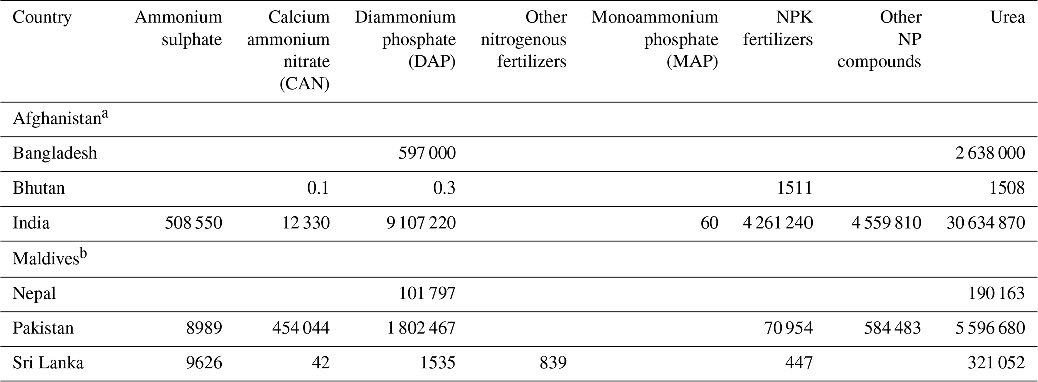
^a For Afghanistan, there are no reported fertiliser totals by product type, only by total nitrogen (N) (92 516 t N used in 2015). ^b For Maldives, there are no reported fertiliser totals by product type, only by total nitrogen (N) (226 t N used in 2015).

Table A2 Nitrogen (N) content of fertiliser types (FAO, 2023).

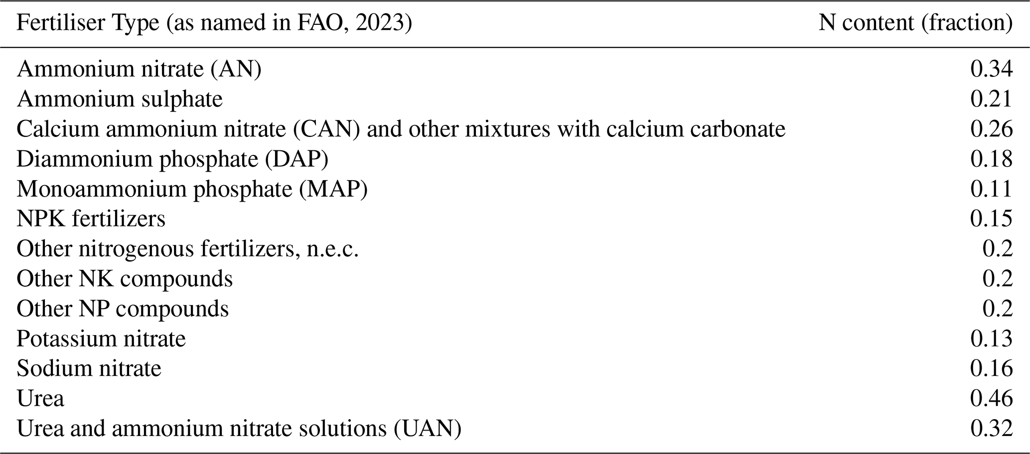
Table A3 Emission factor (EF) by fertiliser type, from EEA (2023) for soils with “normal” (pH < = 7) and “high” (pH > 7) pH. EF is stated as fraction of N lost as NH₃-N.

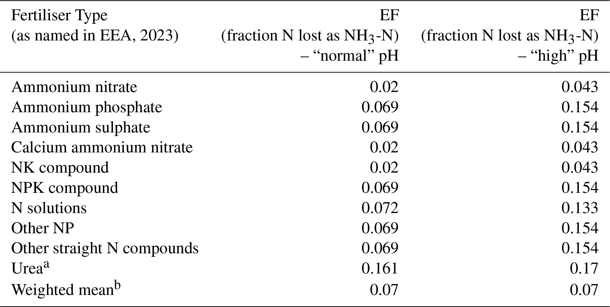
^a Superseded in this study, see Sect. 2.1. ^b The “weighted mean” is a default weighted mean EF across all fertiliser use in 2019 (Tier-1 and Tier-2 mixed method) (see EEA, 2023).

Table A4 Schema to match fertiliser types as named in FAO (2023) and EEA (2023).

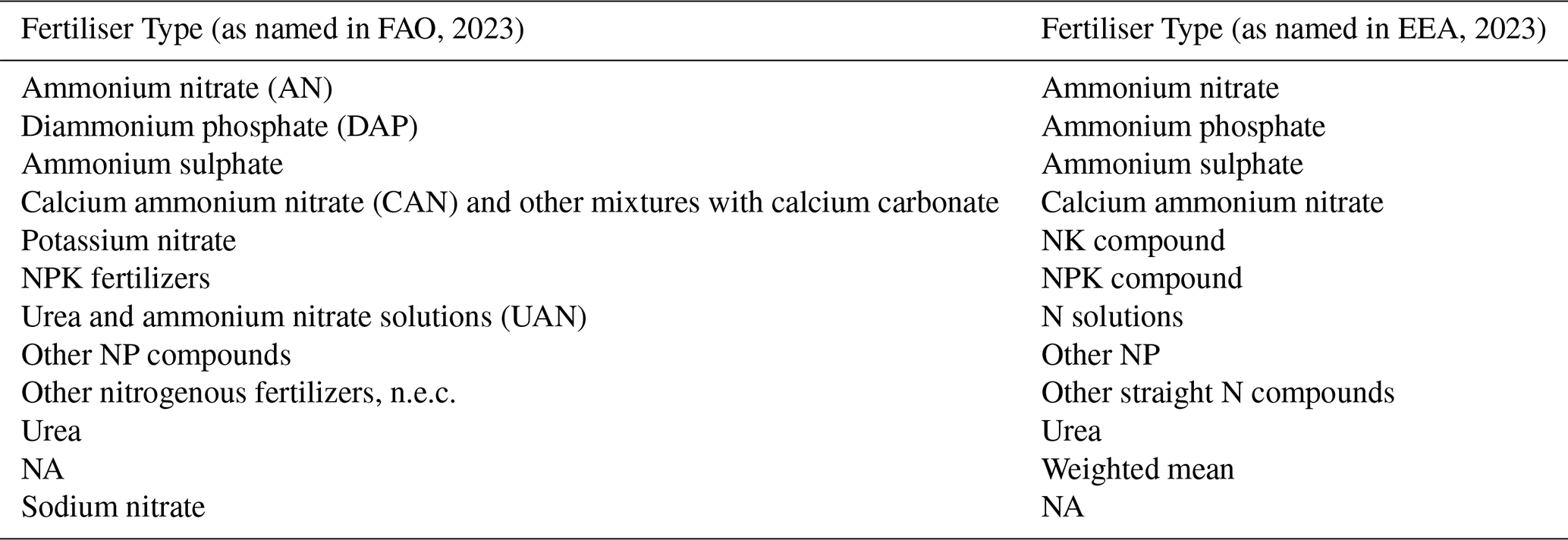
NA – not available.

Table A5 Schema to match crops as named in Cui et al. (2021), EarthStat (Monfreda et al., 2008; Ramankutty et al., 2008), and Table A6 for crop residue and burning estimates.

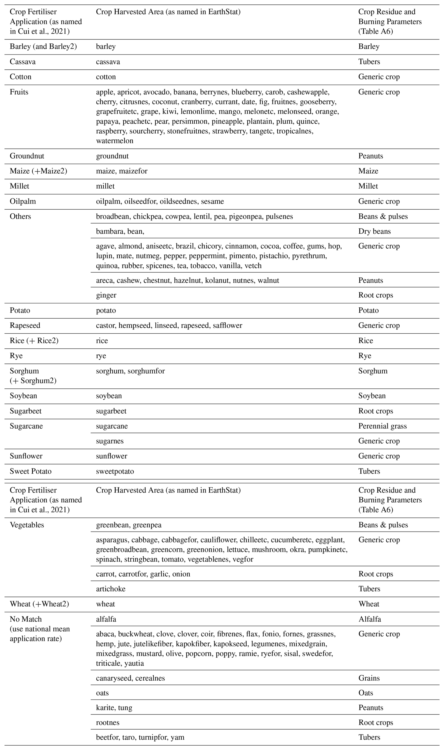
Table A6 Crop parameters used for calculating emissions from crop residues left fields and crop residues burnt, taken from IPCC (2019) and Yevich and Logan (2003) (Fraction Burnt only). Where relevant, numbers in brackets have been superseded by those not in brackets (bold font), but occasionally only for a subset of EarthStat crops (see table notes). See Sect. 2.2 and 2.3.

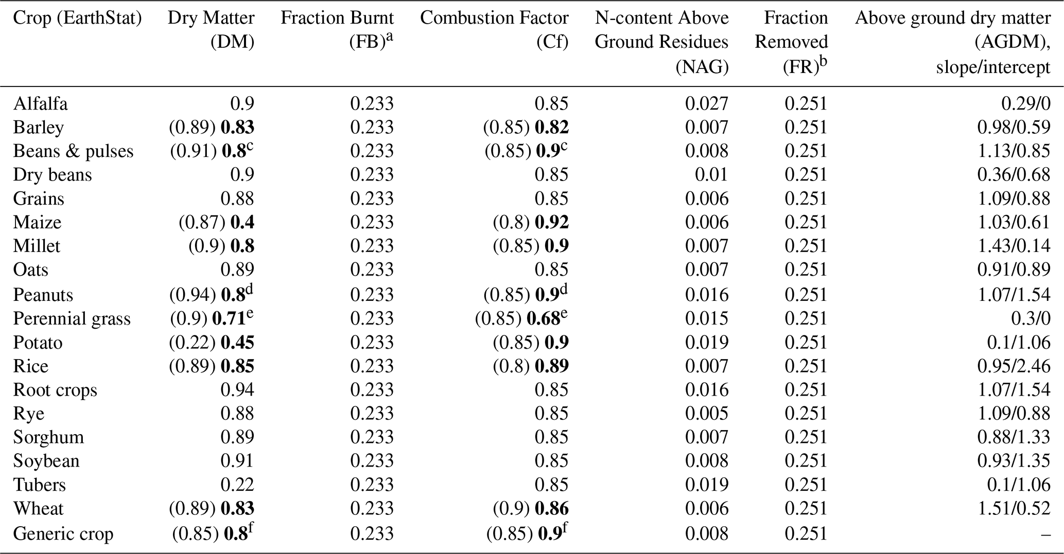
^a For FB: India – Wheat = 0.17, rice = 0.19, sugarcane = 0.25, maize = 0.1, everything else = 0. Pakistan – Wheat = 0.25, rice = 0.53, sugarcane = 0.4, maize = 0.28, barley/bean/groundnut/jute/lentil/millet/potato/rapeseed = 0.233, everything else = 0. Nepal – Barley/bean/groundnut/jute/lentil/maize/millet/potato/rapeseed/rice/sugarcane/wheat = 0.23, everything else = 0. Sri Lanka – Rice = 0.055, Barley/bean/groundnut/jute/lentil/maize/millet/potato/rapeseed/sugarcane/wheat = 0.233, everything else = 0. Bangladesh – Rice = 0.34, Barley/bean/groundnut/jute/lentil/maize/millet/potato/rapeseed/sugarcane/wheat = 0.233, everything else = 0. ^b For FR: India – Rice = 0.77. All else as default. Nepal – Barley/bean/groundnut/jute/lentil/maize/millet/potato/rapeseed/rice/sugarcane/wheat = 0.75. All else as default. ^c Lentils and beans only. ^d Groundnut only. ^e Sugarcane only. ^f Rapeseed and jute only.

Table A7 Lookup table to relate FAOSTAT livestock categories to GLWv4 livestock spatial distributions, used to distribute livestock emission estimates.

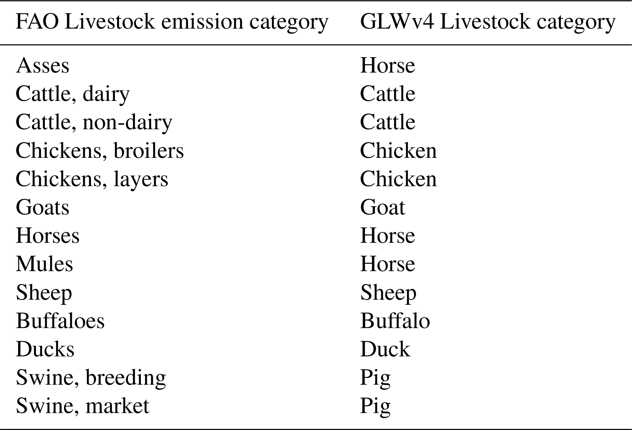
Table A8 Implicit emission factors (EFs) derived from livestock emission calculations (Sect. 2.4). Units are in kg NH₃ Annual Average Population⁻¹ (AAP) yr⁻¹. Emissions were estimated separately for each country, however key emission parameters from the FAO (e.g. Typical Animal Mass and N excretion rates) are assumed to be uniform across the SAARC.