ALTICAP: a new global satellite altimetry product for coastal applications

Observing sea level and its variations is of great importance for many scientific, societal and economic issues. This data paper presents a new coastal high resolution Sea Level Anomaly (SLA) product, ALTICAP (ALTimetry Innovative Coastal Approach Product), derived from along track satellite altimetry. To enable as many coastal applications as possible, collocated altimetric significant wave height and wind data are also provided, as well as quality flags and the geophysical corrections applied to the SLA. Covering all ocean regions between 0 and 500 km from land, and between 66° S and 66° N, this dataset contains 5 years (February 2016 to July 2021) of 20 Hz altimetry measurements from the Jason-3 mission. The altimetric standards and geophysical corrections used to compute the SLA have been selected following a round robin study based on 22 of the most recent algorithms available. The processing solution adopted was a compromise between the capability of each algorithm to provide the best sea level solution over the entire strip between 0 and 200 km from the coast and a guarantee of product continuity in the future.

The comparison of ALTICAP and tide gauge SLA time series shows the ability of the ALTICAP product to capture the coastal sea level variability, with average correlation and root mean square deviation values of 0.74 and 9 cm respectively. On global average, altimetry SLA time series remain 80 % complete up to 9 km from the coast after editing. ALTICAP is a global high resolution altimetry sea level product optimized for coastal applications and ensuring quality continuity up to the open ocean, directly available online. The complete protocol followed during the round robin study (Birol et al., 2023), as well as all the results (https://www.aviso.altimetry.fr/en/data/products/sea-surface-height-products/global/altimetry-innovative-coastal-approach-product-alticap.html, last access: 26 March 2026) and the data (LEGOS et al., 2023, https://doi.org/10.24400/527896/a01-2023.020) are freely available online.

1 Introduction

Satellite altimetry has been routinely measuring sea level variations at nearly global scale for more than 30 years. These observations, freely available and with uncertainties of only a few centimetres, have greatly improved our knowledge of the open ocean and are now a key climate indicator of global warming and an essential component of many operational marine systems (International Altimetry Team, 2021). The number of observations has largely increased over time along with the number of altimetry missions. In 2025, data from eight satellites on different orbits and with different sampling characteristics are processed in near real time (Le Traon et al., 2025). In parallel, data quality has considerably improved, not only thanks to new processing algorithms, but also with innovative altimeter technologies (SAR – Synthetic Aperture Radar, mode and swath altimetry: see for example Moreau et al., 2021 or Fu et al., 2024). As a result, the temporal and spatial resolution of altimetry data has significantly increased. Smaller sea level signals are now observed with these measurements, and larger signals are captured more precisely, with finer space and time granularity. In theory, this should enhance the ability to monitor the dynamic processes in the coastal ocean, which are generally smaller in size and/or faster than those offshore (Robinson and Brink, 2005).

Nevertheless, satellite altimetry encounters different issues that make it difficult to derive accurate geophysical estimates near the shore (see Vignudelli et al., 2011 for a complete review). Firstly, in the nearest coastal band, a few kilometres wide, land and calm water modify radar echoes, leading to complex waveforms that may be difficult to interpret (Gommenginger et al., 2011; Xu et al., 2018). In coastal environments, computing most of the geophysical corrections that are applied to the altimeter measurements (e.g., wet troposphere, ionosphere, sea state bias, inverse barometer, high frequency wind effect, and ocean tides) with the required precision is also challenging (e.g., Andersen and Scharroo, 2011). In practice, they can pollute altimetry sea level estimates up to a few tens of km from the coast (Birol et al., 2025). Finally, operational altimetry products have been optimized for open ocean and/or long-term sea level studies and are not always suitable for coastal applications (e.g., a conservative approach that eliminates a lot of nearshore data, and spatial filtering that removes all noise but also smooths the signal).

Still, altimetry remains an invaluable tool in these regions, where variations in sea level, current and sea state have the greatest socioeconomic impact. This is reinforced by the poor coverage of in situ coastal data on a global scale. For these reasons, radar waveform processing techniques more suitable for near shore conditions have been developed in the recent years (Passaro et al., 2014; Peng et al., 2018; Thibaut et al., 2021). Improved geophysical altimetry corrections and auxiliary parameters for coastal regions are also now available (Fernandes et al., 2015; Carrère et al., 2016; Passaro et al., 2018; Schaeffer et al., 2023). Some of them are progressively introduced into operational processing baselines. As a consequence, the quality and quantity of altimetry data in the coastal zone have considerably increased (Vignudelli et al., 2019; Birol et al., 2021) and some coastal sea level datasets have been released. Some of the most popular coastal sea level altimetry products are (1) X-TRACK developed by CTOH/LEGOS and distributed by AVISO+ (https://doi.org/10.24400/527896/a01-2022.020; Birol et al., 2017), and (2) ALES (Adaptive Leading Edge Sub-waveform, Passaro et al., 2014) produced by DGFI-TUM and distributed via OpenADB (Schwatke et al., 2023; https://openadb.dgfi.tum.de, last access: 26 March 2026). Both are maintained by universities and provide along track cross-calibrated Sea Level Anomalies (SLAs) for most of the available satellite altimetry missions. The former, X-TRACK, is a regional Level-3 product covering almost all the coastal ocean. It is based on an editing and post-processing strategy defined to optimize the completeness and the accuracy of the altimetry SLA in coastal ocean areas. It provides SLA, significant wave height (SWH) and geophysical corrections time series at 1 Hz, i.e., with a spatial spacing of ∼6–7 km between points along the track. The latter, the ALES global Level-3 product, includes a specific waveform retracker applied to high frequency (20 Hz, i.e., ∼0.3 km along the track) altimetry data to help get rid of land contamination in near shore measurements. Nonetheless, there is still a lack for a global multi-mission and high frequency product for the coastal ocean that would combine both tailored retracking and adapted geophysical corrections, and, no less important, would be optimized for a transition to operational production.

In this paper, we present a new coastal high resolution (20 Hz) SLA product, called ALTICAP (ALTimetry Innovative Coastal Approach Product). This along track dataset based on the Jason-3 mission covers the global coastal ocean, from 0 to 500 km from any land surface within the Topex-Jason orbit (66° S to 66° N). It has been computed from recent algorithms selected after a dedicated round robin exercise to guarantee the best possible continuity of quality throughout the coastal zone, between 0 and 200 km from land. Compared to operational altimetry products, it is designed to better catch the temporal and spatial coastal scales and, by providing co-located information in time and space on variations in sea level, waves, and wind, is fitted to monitor and study highly dynamical processes such as coastal currents, eddies, upwellings, and interactions between the ocean and the coast area (including rivers in estuarian regions). The guarantee of product continuity in the future was also a critical parameter in the selection, with the objective to further extend the product and include additional altimetry missions.

This data paper is structured as follows: Sect. 2 describes the method and input data for the study; Sect. 3 presents the data processing, the results of the product validation and the comparison to the X-TRACK coastal reference product; Sect. 4 provides detailed information on the resulting dataset and its distribution. The article closes with a conclusion and some perspectives in Sect. 5.

2 Method and input data

2.1 Method

Satellite altimetry observes sea level variations by measuring the round-trip time taken by radar pulses from the instrument to the surface at nadir. Knowing the speed of these pulses (the speed of light), we can compute the distance between the satellite's center of mass and the reflected surface, called the altimeter range. Over the ocean, going from the range to the SLA requires knowledge of auxiliary information (e.g., satellite altitude; atmospheric and geophysical corrections; time-average of the height of the ocean surface). Finally, the SLA is computed according to Eq. (1):

$$\begin{array}{}\text{(1)}& \begin{array}{rl}\mathrm{SLA}& =\mathrm{Altitude}\mathrm{of}\mathrm{satellite}-\mathrm{Altimeter}\mathrm{range}\\ & -\mathrm{Ionospheric}\mathrm{correction}-\mathrm{Dry}\mathrm{tropospheric}\mathrm{correction}\\ & -\mathrm{Wet}\mathrm{tropospheric}\mathrm{correction}-\mathrm{Sea}\mathrm{state}\mathrm{bias}\mathrm{correction}\\ & -\mathrm{Solid}\mathrm{earth}\mathrm{tide}\mathrm{correction}-\mathrm{Geocentric}\mathrm{ocean}\mathrm{tide}\mathrm{correction}\\ & -\mathrm{Geocentric}\mathrm{pole}\mathrm{tide}\mathrm{correction}-\mathrm{Dynamic}\mathrm{atmospheric}\mathrm{correction}\\ & -\mathrm{Internal}\mathrm{tide}\mathrm{correction}-\mathrm{Mean}\mathrm{sea}\mathrm{surface}\mathrm{height}.\end{array}\end{array}$$

Each of the terms of Eq. (1) will be called “SLA component” hereinafter. The accuracy of the resulting SLA depends on the quality of each of these terms, which are derived from either numerical or empirical models, and from altimetry or auxiliary observations. For most of these correction terms, different solutions exist. In some cases, algorithms specifically designed for the coastal environment are available, such as the GPD+ (GNSS derived Path Delay, Fernandes et al., 2015) wet troposphere correction and the ALES retracker (Passaro et al., 2014).

Here, we take advantage of the results of a companion study (Birol et al., 2025) to build the new global coastal ALTICAP product. In Birol et al. (2025), we carried out a round robin study to better understand the sources of uncertainties linked to the processing algorithms in the sea level computation when approaching the coast. We intercompared the SLA estimates obtained with a set of 21 processing solutions for different SLA components (see Sect. 2.2), in order to study how the uncertainties in each solution are reflected in the calculation of the SLA data as we get closer to the coast. In the present work, we add a recent algorithm (FES2022b ocean tide solution, Lyard et al., 2021) for a total of 22 processing solutions, and use different metrics to objectively compare the relative performance of the different algorithms in terms of coastal SLA computation. For each SLA component analyzed, we then choose the algorithm that provides the most accurate SLA in the whole coastal domain between 0 and 200 km offshore, and that also ensures continuity with the open-ocean standard SLA products. A third selection criterion is the availability (or possibility of availability without too much effort in the future) of the algorithms for several missions, as one important objective is to extend the ALTICAP dataset in the past with the Jason-1 and Jason-2 missions, and up to the present day with the Sentinel-6-MF mission. To verify that the results were consistent among several altimetry missions, the round robin study included the Jason-2 and Jason-3 missions, considering three years (i.e., 111 cycles) of data for each of them: 27 September 2013 to 22 September 2016 for Jason-2, and 17 February 2016 to 22 February 2019 for Jason-3.

2.2 Altimetry algorithms

The operational sea level products (i.e., the Level-2 Geophysical Data Record or GDR products) have been our starting dataset in this work. We collated all the data into the CNES (French Space Agency) internal altimetry database that contains all the operational Jason-2 and Jason-3 GDR products (CNES, 2024a, b). We added external solutions and project-oriented datasets that were made available for this study.

Some of the SLA components of Eq. (1) were not included in the round robin because only one solution was available for them (Altitude of the satellite, Dry Tropospheric Correction, Dynamic Atmospheric Correction, and Internal tide Correction). The Solid earth tide height and the Geocentric pole tide height were also discarded because they are considered very accurate and non-critical for coastal sea level calculations (Andersen and Scharroo, 2011). For the other components, the main criterion to select the algorithms was the availability of the corresponding dataset at global scale and for the whole study time period (i.e., 27 September 2013 to 22 February 2019). A few exceptions have been made for specific reasons:

The ALES altimeter range and the associated Sea State Bias (SSB) correction, both obtained from the ALES retracking algorithm, come from the ESA CCI Coastal Sea Level product (Cazenave et al., 2022). Although they are not global, they cover a large part of the coastal ocean (see Fig. 1 of the aforementioned article). Because the ALES retracking algorithm was specifically developed for coastal altimetry, the study would not have been complete without its inclusion. As a consequence, all the altimeter range and SSB solutions selected in this study have been evaluated only where ALES data are available.

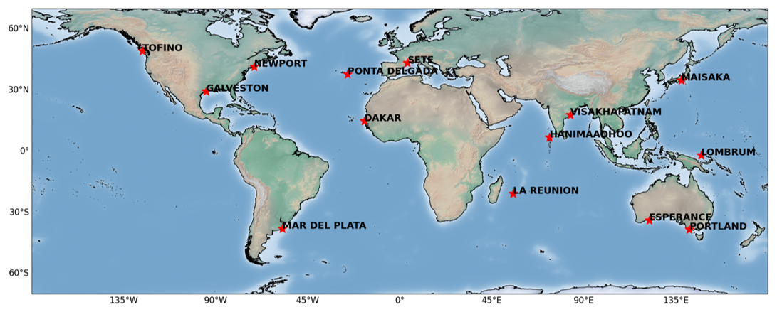
Figure 1 Locations of the 14 tide gauge stations (red stars) used for the validation of the ALTICAP dataset. Background map from Natural Earth.

Although they only cover a limited geographical domain by definition, regional tidal corrections made available by CNES/Noveltis for the Mediterranean Sea, North East Atlantic (NEA) and Eastern Australia regions have been included in the round robin exercise to explore and analyze their potential for coastal altimetry, compared to global solutions. Regional analyses were thus specifically performed for the ocean tide corrections.

Regarding the SSB correction, some of the new algorithms were available only for Jason-3 (MLE4 2D 20 Hz, MLE4 3D 20 Hz, and Adaptive 3D 20 Hz). Given that the SSB is identified as one of the critical issues in coastal altimetry, it was decided to include the performance analysis of these algorithms in this study. Hence, the evaluation of the SSB algorithms was performed only for the Jason-3 mission over the considered period.

Finally, the SLA components and algorithms used in this round robin are listed in Table 1. Note that other global ocean tide solutions are available, in addition to those included in this study, such as DTU16 (Cheng and Andersen, 2011), GOT4.10c (Ray, 2013), and TPX09 (Egbert and Erofeeva, 2002). To avoid any overrepresentation of ocean tide correction solutions in the round-robin exercise, compared to other SLA components, a specific pre-analysis was done on tidal models and led to the selection of five solutions. The results of this pre-round-robin analysis are available in a dedicated report on the AVISO+ website (Cancet and Fouchet, 2022).

Table 1 SLA components included in the round robin exercise (column 1), with the list of algorithms tested for each one (column 2). The reference algorithms currently used in operational sea level products for each component are in bold. The fields marked with ^a were provided at 1 Hz only and have been linearly interpolated to 20 Hz for the purposes of this study; the fields marked with ^b have been specifically interpolated at 20 Hz from the native grids for this study; the others were at 20 Hz. GDR is the official Geophysical Data Record product distributed by the space agencies (version D for Jason-2 and version F for Jason-3).

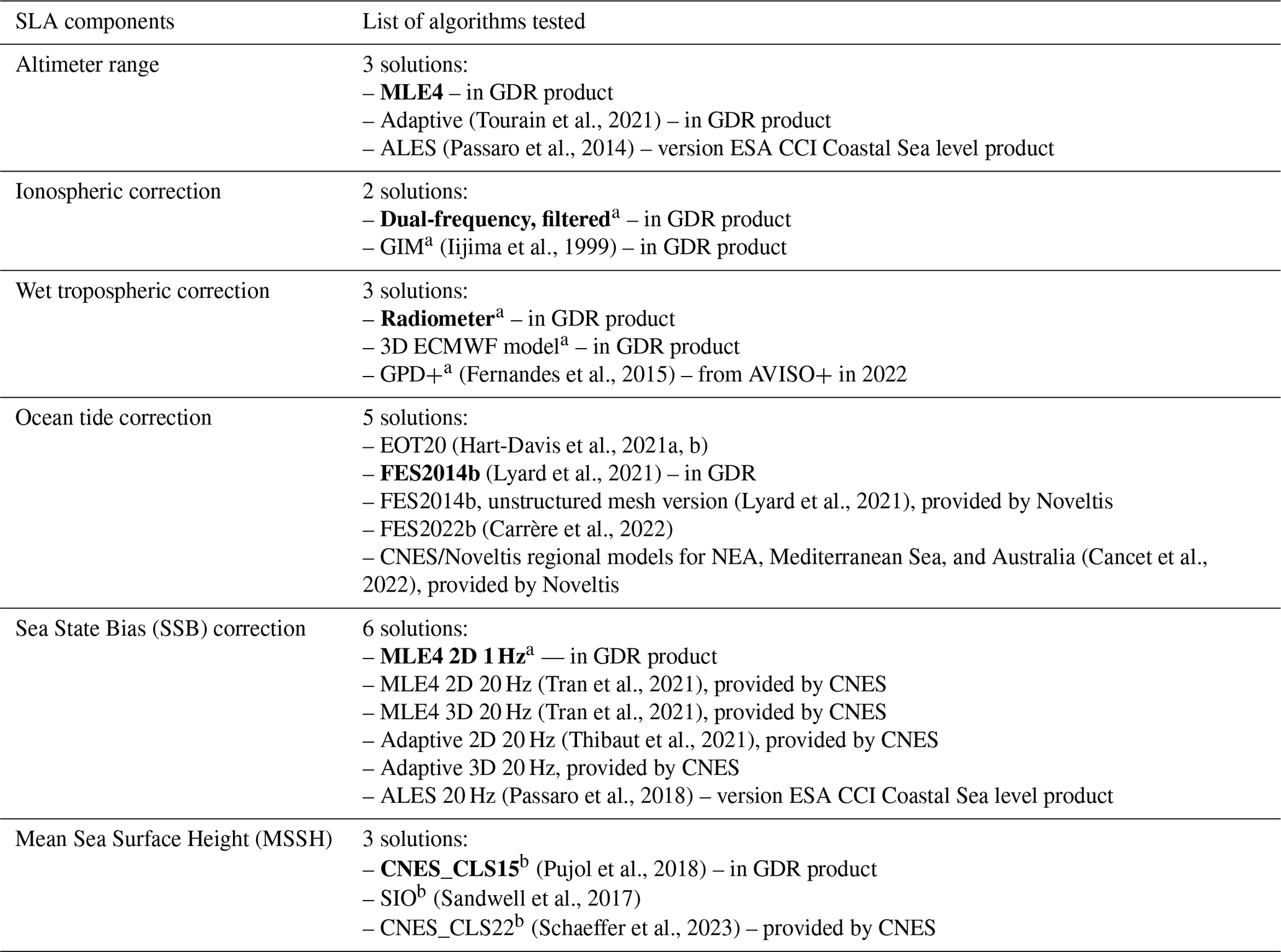
A reference SLA solution was computed using the reference algorithms available in the operational GDR products (underlined in Table 1). We then produced new SLA datasets by changing one SLA component at a time, considering the different algorithms available. For example, we considered two different ionospheric corrections (GIM and dual-frequency correction), hence resulting in two different SLA solutions for the ionospheric correction. The only exception was for the range and SSB that are strongly interlinked as they both come out of the retracking algorithm. In that case, we produced SLA estimates pairing the range and SSB solutions together (i.e., no mixing MLE4 range with ALES SSB for example). We finally obtained 22 SLA datasets that have all been evaluated using the same metrics through the round-robin exercise.

2.3 Tide gauge data

Hourly tide gauge data are used for validation and comparison. The data have been retrieved from the UHSLC (https://uhslc.soest.hawaii.edu/data/, last access: 15 October 2021) and SHOM (https://data.shom.fr, last access: 15 October 2021) databases. Among all available tide gauge stations at global scale, we selected a subset of 14 stations (Fig. 1) scattered across the world coastal ocean and in both hemispheres. The selection criteria were as follows: (1) the temporal coverage of the tide gauge time series must cover the Jason-3 period without significant gaps or abrupt changes (instrumental drift, calibration issue, etc. …); (2) the distance between the tide gauge station and the altimetry track must be smaller than 50 km when considering only altimetry points located less than 20 km off the coast. Note that for some stations, some additional selection was done on the altimetry side to avoid comparing sea level observations in regions with different ocean dynamics regions (e.g., data located in a lagoon for Galveston, in narrow fjords for Tofino, or on the opposite side of a peninsula for Dakar).

To compare the altimetry and tide gauge sea level measurements, the tidal signal has been removed from the tide gauge sea level time series using a harmonic analysis approach. The effect of atmospheric pressure and wind on the tide gauge sea level has been subtracted using the same correction as for the altimetry observations (Dynamic Atmospheric Correction from MOG2D solution, LEGOS/CNRS/CLS, 1992; Carrère and Lyard, 2003).

2.4 External altimetry product

For validation purposes, ALTICAP SLA time series are compared with those of an equivalent coastal sea level product. From the two most popular products mentioned above, we have chosen X-TRACK (CTOH, 2023; Birol et al., 2017) since it is the closest in terms of content. It is also the most widely used in coastal studies, with over 170 publications. X-TRACK is a Level-3 product, which means that along track SLA are projected onto reference ground-tracks. It is computed by LEGOS/CTOH starting from the Level-2 Plus (L2P) CNES products. More than 30 years of data are available and are distributed by AVISO+. X-TRACK is a 1-Hz product (i.e., with a 6 to 7 km posting rate) and has then a coarser spatial resolution than ALTICAP (20 Hz, i.e., 350 m posting rate) in the along-track direction. Given that the ALTICAP dataset only includes data from the Jason-3 mission from February 2016 to July 2021 (at the time of writing), all the following comparisons described in Sect. 3.3 are only performed over this period.

3 Data processing and validation

This section presents the algorithm selection that led to the computation of the ALTICAP product, the different data processing steps, and the validation of the dataset.

3.1 Algorithm selection

The algorithm selection was based on the aforementioned round robin study dedicated to the impact of processing algorithms in the coastal sea level computation. The complete protocol followed during this work (Birol et al., 2023), as well as all the results, are available online: https://www.aviso.altimetry.fr/en/data/products/sea-surface-height-products/global/altimetry-innovative-coastal-approach-product-alticap.html (last access: 26 March 2026). As we have addressed several scientific objectives within this round robin and evaluated 21 algorithms at global scale and in three regions, both for Jason-2 and Jason-3, the total number of computed diagnostics reached several hundreds. Only a summary of the information that led to the selection of the algorithms used in the ALTICAP calculation and the result of this selection are provided in this section; the main analyses that enabled us to select the algorithms are presented in Appendix A. Note that in the results presented here, a 22nd algorithm was considered (the FES2022b ocean tide correction), as previously mentioned.

The basic principle of the round robin study was to compare all the selected SLA components and algorithms of Table 1 using the same metrics, so their impact on the coastal sea level computation can be assessed in the same way. The study has been organized by SLA component. At global scale, the different algorithm solutions have been intercompared between 0 and 200 km from the coast. It has been done in terms of data availability (spatial pattern of data availability, data availability as a function of the distance to the coast) and general statistics (mean, standard deviation, distribution of values). Then, the impact on the SLA calculation has been analyzed for each algorithm of a component, using similar metrics. The same diagnostics have been computed at regional level, for the Mediterranean Sea, the North-East Atlantic Ocean, and eastern Australia. Additional analyses have also been performed at coastal scale, with a comparison to independent tide gauge observations.

As the Level-2 altimetry products are provided at the point-measurement locations, which differ from one cycle to the other, all the along-track sea level components and SLA values were binned along mean ground tracks of the Jason missions with a resolution of 20 Hz (i.e., 0.3 km), in order to ease the computation of the along-track statistics. No editing was applied to the SLA components and all values available in the dataset were used. SLA values outside the window [−3; 3 m] were systematically discarded everywhere. In the Mediterranean Sea, associated with generally lower SLA variations, a narrower window of [−1; 1 m] was applied. For each SLA point time series, values outside a 4 sigma window have also been removed from the computations, sigma being the standard deviation of the SLA time series. Finally, altimetry points were binned considering their distance to the coast. To ensure robust global or regional statistics, we considered a fixed number of altimetry points in each bin, with the bin size varying from about 300 m at the coast to 1.2 km at 200 km from the coast. For the comparison between altimetry and in situ SLAs, the nearest satellite track to each tide gauge station was selected. Only altimetry data located at a distance from the coast smaller than 20 km, and less than 50 km from the nearest reference tide gauge, were used.

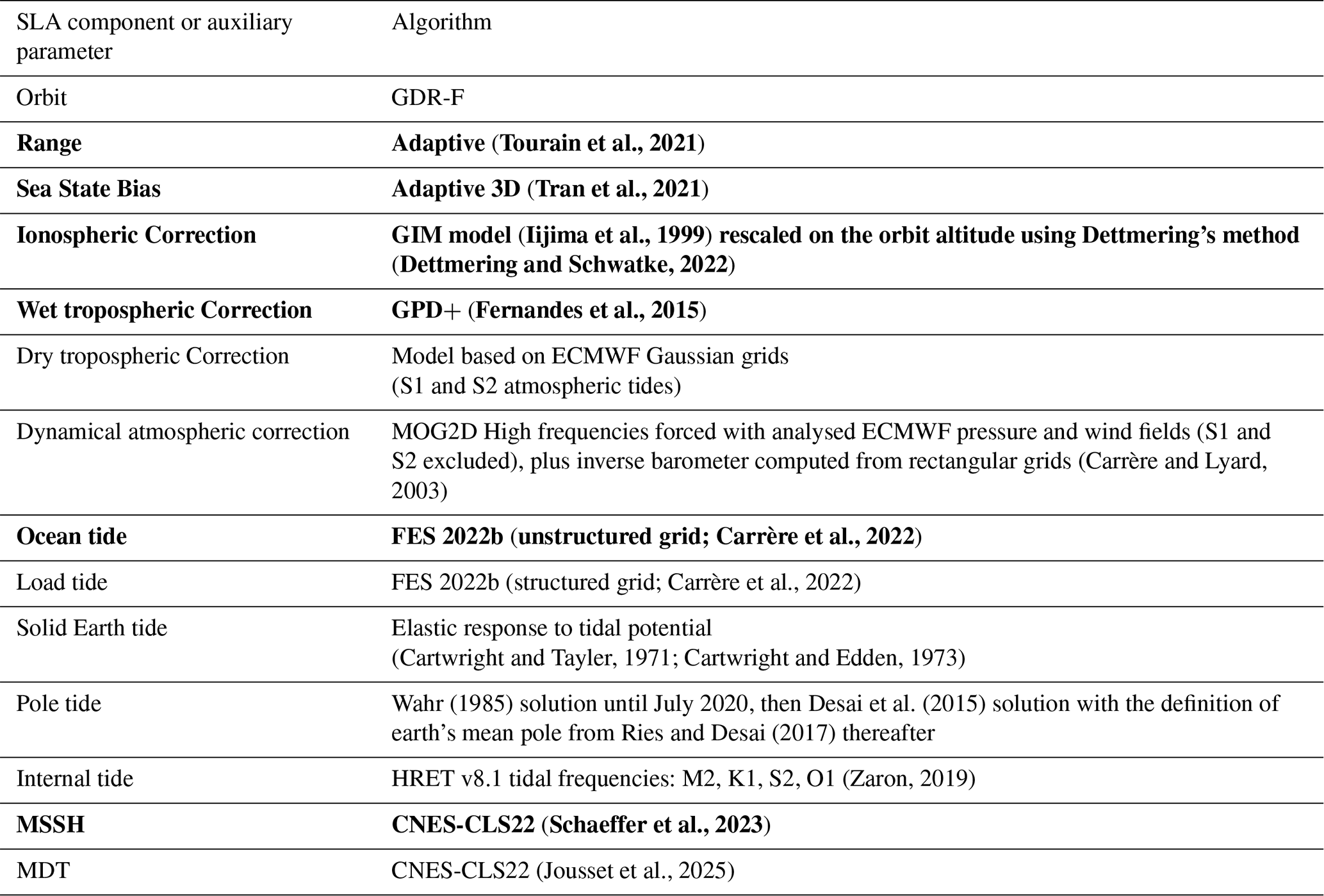
The final choice of algorithms used to compute the ALTICAP SLA dataset is summarized in Table 2. The SLA components selected in the context of the round robin, following all the criteria described in Sect. 2.1, are indicated in bold. The other parameters correspond to the environmental and geophysical altimetry corrections that were not included in the round robin but need to be applied to the SLA.

Table 2 Altimetry algorithms used in the ALTICAP product processing. The algorithms in bold were selected through the round robin process.

3.2 Data processing

The ALTICAP processing system starts from the 20Hz Jason-3 altimeter along-track measurements, in delayed time, provided in the GDR products. In order to generate the SLA data, the altimetry observations follow a processing chain with several steps: acquisition and pre-processing, quality control, calibration, and SLA computation.

A database is built from the GDR products with all the 20 Hz along-track data that are needed to compute the SLA: time, range, orbit, information of validity, environmental and geophysical corrections, auxiliary parameters. The components that are available only at 1 Hz in the GDRs are either specifically computed or interpolated at the 20 Hz frequency along the track from the native grids (MSSH, SSB), or interpolated from 1 to 20 Hz through a linear method (e.g., ionospheric and wet tropospheric corrections). The SLA is then computed at each 20 Hz measurement point along the altimeter ground track using Eq. (1) and the standards described in Table 2. An additional correction (called inter_mission_bias) has been applied to remove systematic differences between altimetry missions, yielding SLA time series consistent with those delivered by CMEMS (https://doi.org/10.48670/moi-00146, EU Copernicus Marine Service Information (CMEMS), 2024). Finally, the mono-mission Orbit Error Reduction (OER) algorithm (Le Traon and Ogor, 1998) is used to reduce orbit errors through a global minimization of the SLA differences observed at crossover points.

The processing continues with quality control of the altimetry data and geophysical corrections in order to compute the validation flag that allows to select valid ocean data. Several criteria are used: thresholds values set on the SLA and the collocated significant wave height (SWH) estimates (abs(SLA) < 2 m and SWH < 15 m), detection of points contaminated by the presence of sea ice using a combination of the OSISAF sea ice concentration (EUMETSAT, 2022) and the GDR ice flag, identification of rain cells and specular reflections (sigma0 backscattering blooms). The along track coherence of SLA data is then verified using a variable nσ criterion, where σ is the standard deviation of the SLA and the value of n is modulated regionally using an estimate of the ocean variability derived from merged Level-4 DUACS products. This allows for the natural variability of each ocean region to be taken into account in the detection and removal of outliers. An additional data quality criterion aims to flag small scale SLA outliers. This criterion is based on low pass filtered SWH values over a 11 km running window, and flags all the SLA values where the filtered SWH amplitude is larger than 2 m.

The distributed ALTICAP dataset contains the SLA data at all points located over the ocean and a validation flag that corresponds to the combination of all the editing criteria described above. Users can thus either apply the flag to edit the dataset following the described strategy, or create their own editing methodology and associated flag based on the complete ALTICAP dataset.

3.3 Validation

In this section, we present the main results concerning the validation of the ALTICAP sea level dataset. Two SLA versions are used: without and with the validation flag applied, respectively called “raw' and “edited” hereinafter.

First, we evaluated the impact of the validation flag on the SLA standard deviation (SD) and on the data availability. In practice the latter is measured by the percentage of data with a value in the SLA time series. These diagnostics are represented as a function of the distance to the coast (Fig. 2) and in the form of a map over the whole domain covered by the ALTICAP dataset (Fig. 3). Without the flag, SD values increase sharply within 10 km from the coast, reaching several meters, due to an increasing number of outliers in the SLA as we approach land. The time series remain 80 % complete up to an average of 4.3 km from the coast at global scale. When applying the validation flag, the SD values of the ALTICAP SLAs are strongly reduced in the last 10 km off the coast, from several meters to about 10 cm (see Fig. 5 in the next section for a similar plot with a different vertical range). The amount of edited data in the SLA time series decreases below 80 % up to 8.7 km from the coast in global average. The areas where ALTICAP data are the most edited (Fig. 3b) are the polar regions, which are affected by the seasonal presence of sea ice (e.g., Southern Ocean, Hudson Bay, Canadian coast, Okhotsk Sea, coast of Alaska), and the tropical band (particularly the South-East Asian Seas) that is strongly affected by rain cells.

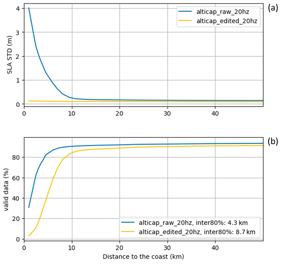
Figure 2 Standard deviation (a) in meters, and percentage (b) of SLA data as a function of the distance to the coast, for the raw (blue) and edited (orange) ALTICAP SLAs. Inter80 % refers to the distance to the coast at which 80 % of data availability is obtained.

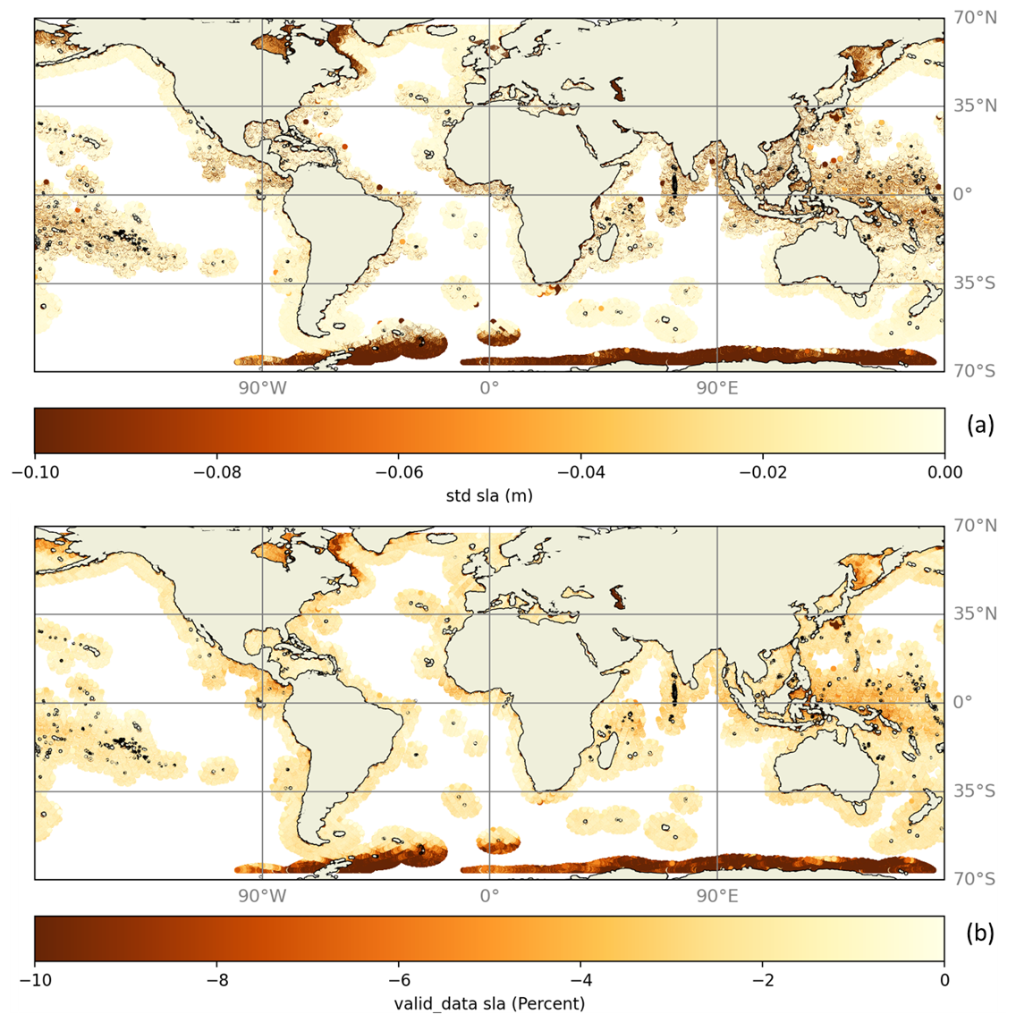
Figure 3 (a) Difference of ALTICAP SLA SD (in meters) before and after the validation flag is applied (edited-raw). (b) Percentage of SLA data lost when the validation flag is applied.

For further analysis, we use the tide gauge data described in Sect. 2.3 as a reference. Here, only altimetry data within a distance of 20 km from the coastline and 50 km from the tide gauge stations are used. For each in situ station, we compute the ALTICAP data availability. We also calculate the SD of both ALTICAP and tide gauge SLAs, the standard deviation of the difference between ALTICAP and tide gauge data (RMSD) and the correlation between the two types of SLA data. The results are presented for each tide gauge in Fig. 4. Maps showing the comparison at each tide gauge station are provided in Appendix B, illustrating the diversity of situations covered with the tide gauge dataset. In global average, the raw ALTICAP SLA data nearest to the tide gauges are ∼94 % complete and have a SD value of 0.48 m. When comparing to tide gauges, the mean RMSD is 0.47 and the mean correlation > 0.5. In Fig. 4, the comparison to the tide gauge observations clearly shows the improvement brought by the use of the validation flag on the ALTICAP SLA dataset. The percentage of SLA data available near the tide gauges falls to ∼86 % on global average. The loss of data depends of the tide gauge, but there is always more than 70 % of edited ALTICAP data available at the considered altimetry points, close to the in situ stations. In return, here again, the SD of the ALTICAP SLA estimates is strongly reduced when applying the validation flag, at all tide gauge stations. The RMSD and the correlation to each tide gauge also improve significantly.

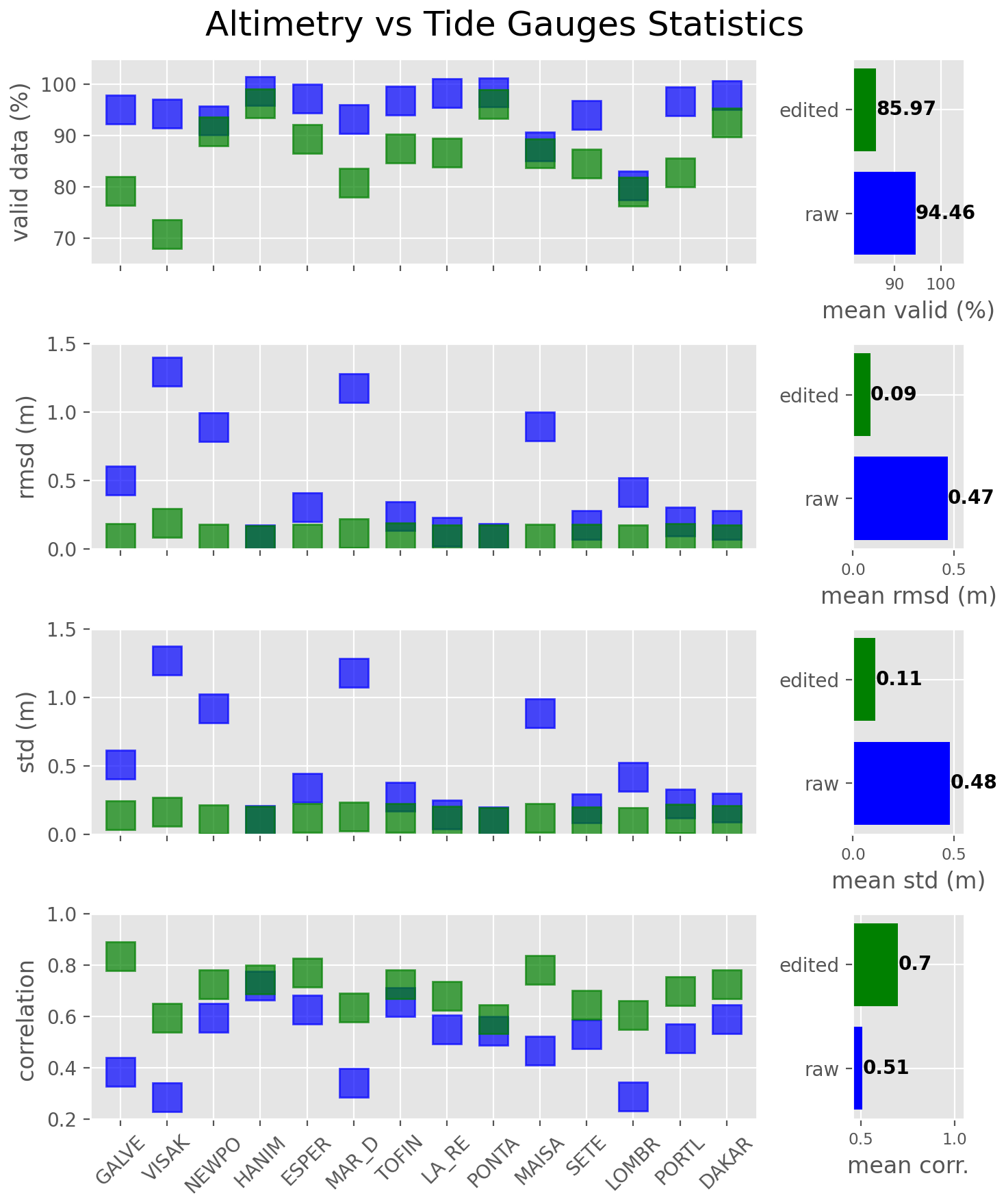
Figure 4 Mean statistics from the comparison between the raw (blue) and edited (green) SLAs of the ALTICAP product and the selected tide gauges (for brevity, only the first 5 letters of the names are shown). The statistics have been computed for each altimetry point located at less than 20 km from the coast and less than 50 km from the tide gauge station, and then averaged for each tide gauge. They are presented for each tide gauge (left panels) and then averaged on a global scale (right panels).

These results demonstrate the efficiency of the validation flag to edit outliers in the ALTICAP SLA dataset and provide high-quality sea level observations. As previously mentioned, this validation flag can also be revisited by users who may want to select data differently and/or apply a local editing, as the raw data are available in the ALTICAP dataset.

3.4 Comparison to a reference altimetry product

In this section, we compare the edited ALTICAP 20 Hz SLAs with the X-TRACK 1 Hz reference product described in Sect. 2.4. Both products show similar behaviors in terms of SD and data availability as we approach the coast (Fig. 5): in the last 10 km from land, the SD increases significantly and the percentage of data decreases rapidly. The ALTICAP product shows a SD about 2 cm higher than that of the X-TRACK product, which is expected due to the higher frequency of the ALTICAP product (20 Hz vs. 1 Hz for X-TRACK), given that 1 Hz data are constructed by averaging 20 measurement points at 20 Hz. This is confirmed when looking at the 20-point averaged ALTICAP product (called “ALTICAP edited 1 Hz” in Fig. 5), which provides a similar level of variability as the X-TRACK 1 Hz product. Between the coast and 10 km offshore, the ALTICAP product provides more valid data (about 10 %), compared to the X-TRACK product.

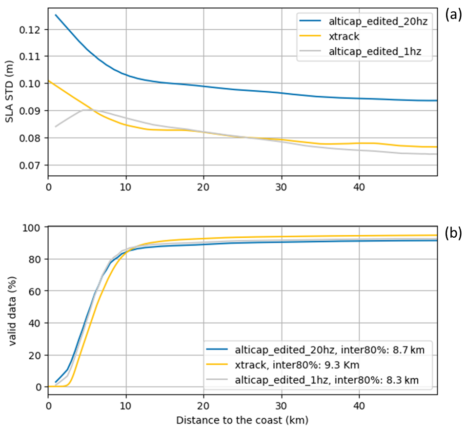
Figure 5 Standard deviation in meters (a) and percentage of valid data (b) as a function of the distance to the coast for the X-TRACK SLAs (blue), the edited 20 Hz ALTICAP SLAs (orange) and the edited 20 point averaged ALTICAP SLAs (grey). Inter80 % refers to the distance to the coast at which 80 % of valid data availability is obtained.

The maps of SLA SD (Fig. 6) show that both products are in very good agreement, with very similar high-variability patterns generally corresponding to regions of strong western-boundary ocean currents (e.g., Gulf Stream, Kuroshio, Agulhas Current, East Australian Current, Brazil Current …). This figure also highlights the difference in terms of spatial coverage between the two products: X-TRACK is processed by regions, covering almost all the global coasts and largely spanning into the open ocean in some cases, while ALTICAP is strictly defined so as it covers the whole global coast up to 500 km offshore.

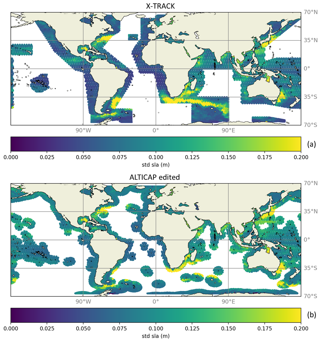
Figure 6 Standard deviation of the SLAs (in meters) at each altimetry point for the X-TRACK 1 Hz dataset (a) and the edited ALTICAP 20 Hz dataset (b).

As in the previous section, we also compare the two altimetry products with the SLA observations from the 14 tide gauge stations, using the same statistics (Fig. 7). The results are generally in the same range for both products. For this small selection of altimetry points, located less than 20 km from the coast and less than 50 km from the tide gauge stations, X-TRACK provides slightly more complete time series than ALTICAP (∼89 % against 86 %, on average over all stations). However, these complete X-TRACK time series may be located a little less close to the coast than ALTICAP ones, as seen on global average in Fig. 5. The comparison to tide gauge data is slightly better for the X-TRACK product (lower RMSDs, higher correlations), which is expected as it is a 1 Hz product, by construction less noisy than the ALTICAP 20 Hz product. However, the difference in statistical results is very small compared to the difference in resolution and would probably be largely offset by low-pass spatial filtering along the track (see Birol and Delebecque, 2014 for an illustration of the advantage of this type of approach, and Fig. 5 for the impact of a simple 20-point averaging on the ALTICAP 20 Hz product). The standard deviation of the in situ SLAs at each tide gauge station is also shown (in purple in Fig. 7) and is in the same order of magnitude as those of the two altimetry products. In the case of the tide gauge station of Visakhaptnam (“Visak” in Fig. 7), we observe a larger standard deviation of SLA for the in situ data than for the two altimetry datasets (∼25 cm). This is due to some drift in the tide gauge data over the period mid-2019 to mid-2021. We can note that even with the less noisy X-TRACK 1 Hz product, the correlation with some tide gauge stations can be lower, around 0.6 (Mar del Plata and Lombrum), which is probably due to the configuration and the local dynamics, as tide gauges and altimeters can observe very different SLA dynamics within a few kilometers, particularly once dominant signals such as tides and wind and atmospheric pressure forcing are removed. For more details on the local configurations, maps of the correlations between along track altimetry (ALTICAP and X-TRACK) and tide gauges are provided in Appendix B for each station.

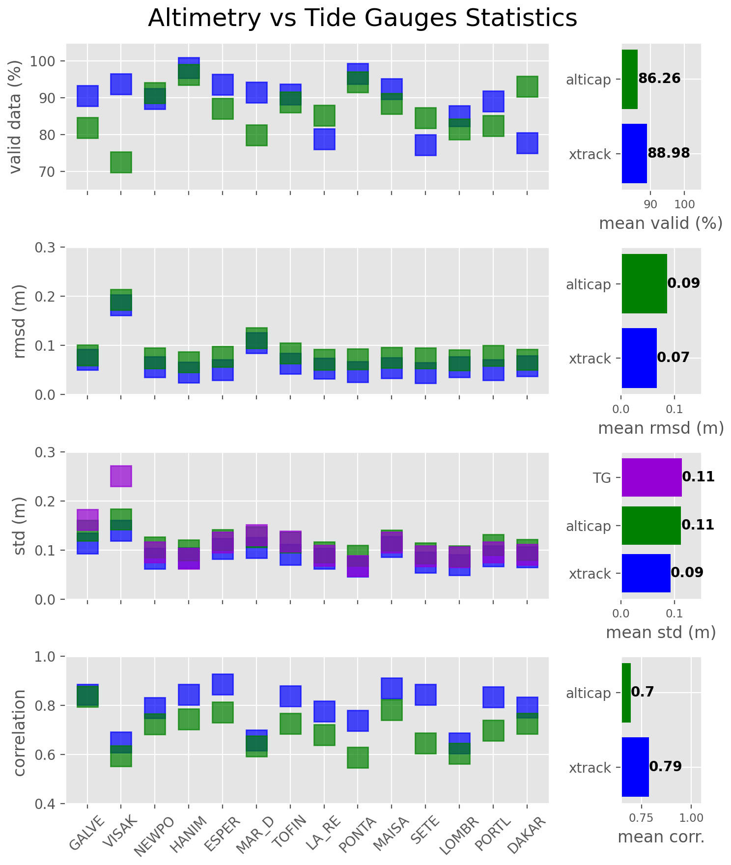
Figure 7 Mean statistics from the comparison between the edited ALTICAP (green) and X-TRACK (blue) SLAs and the selected tide gauges (for brevity, only the first 5 letters of the names are shown). The statistics have been computed for each altimetry point located at less than 20 km from the coast and less than 50 km from the tide gauge station and then averaged for each tide gauge. They are represented by tide gauge (left panels) and then averaged on a global scale (right panels). The standard deviation of the tide gauge SLA is also shown in purple.

When zooming in over a particular region, like the Bay of Biscay (Figs. 8–11), one can see the local added value brought by the ALTICAP product in terms of altimetry point density (20 Hz) and coastal data availability, compared to the X-TRACK coastal product. We show here the example of the Jason-3 track 213, which reaches the French Atlantic coast in the area of the Pertuis Charentais, a shallow region characterized by flat bathymetry and several islands (encircled in red in Fig. 8a). In this region, there is no data available in the X-TRACK product north of 46.2° N (Fig. 8b), while there are data in ALTICAP for more than 60 % of the cycles between 46.25 and 46.3° N, between the island of Ré and the French continental coast (Fig. 8a for one particular date, and Fig. 9b for an overview of the period 2019–2020). In Fig. 9, one can also note the very good agreement between the along track SLA of the two products, from one cycle to the other. Similar results are obtained with the along track significant wave heights (SWH) derived from altimetry that are also provided in the two products (Fig. 10a and b). Note that no validation flag is provided in ALTICAP for this variable, hence the very coastal SWH data should be handled carefully by the users, especially in the very shallow region of the Pertuis Charentais taken here as an example. Similarly, the altimeter wind speed at the ocean surface is also available in the ALTICAP product (Fig. 10c), unlike the X-TRACK product. Figure 11 shows the time series of the three ALTICAP variables (SLA, SWH and wind speed) at one point along this track (at latitude 46.0° N) for the whole period available in the product (2016 to 2021). Having the three variables (SLA, SWH and wind speed) collocated in space and time within the same product enables easy and direct analyses, for example to identify storm events, like in mid-February 2019, in early November 2019 and in early December 2020 (large SWH and wind speed in Figs. 10 and 11).

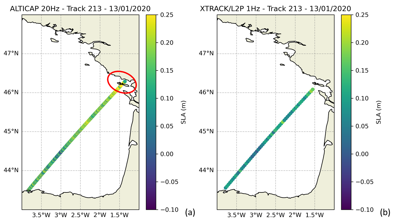
Figure 8 SLA (in meters) from the edited ALTICAP 20 Hz product (a) and the X-TRACK 1 Hz product (b) along the Jason-3 track 213, for cycle 142 (13 January 2020) in the Bay of Biscay (French Atlantic coast). The area of the Pertuis Charentais where the ALTICAP product brings additional data compared to the X-TRACK product is encircled in red.

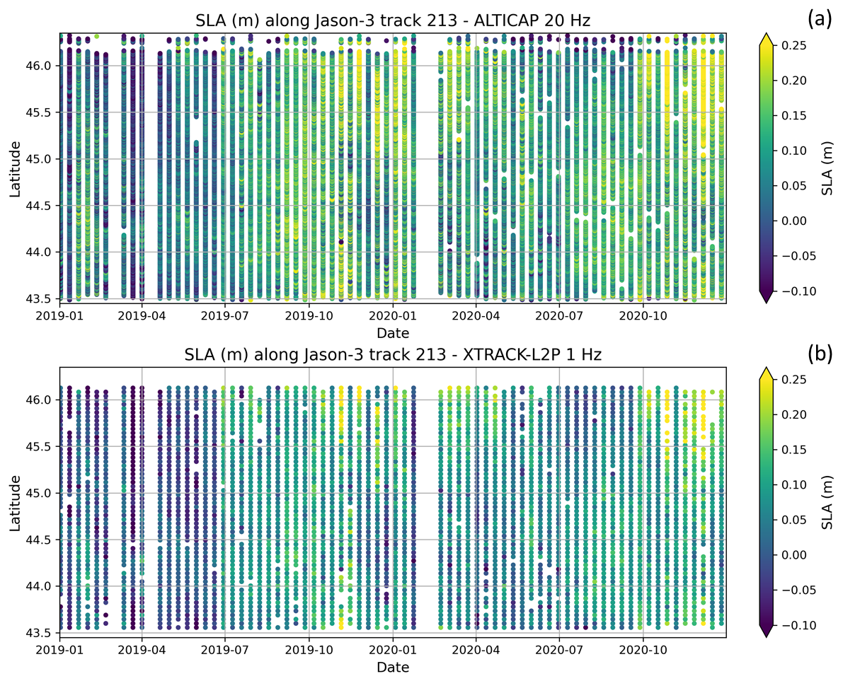
Figure 9 Time-latitude diagrams of the SLA from the X-TRACK 1 Hz product (a) and the edited ALTICAP 20 Hz product (b), along the Jason-3 track 213 in the Bay of Biscay, for the time period 2019–2020. Note the increased data availability north of latitude 46° N in the ALTICAP product.

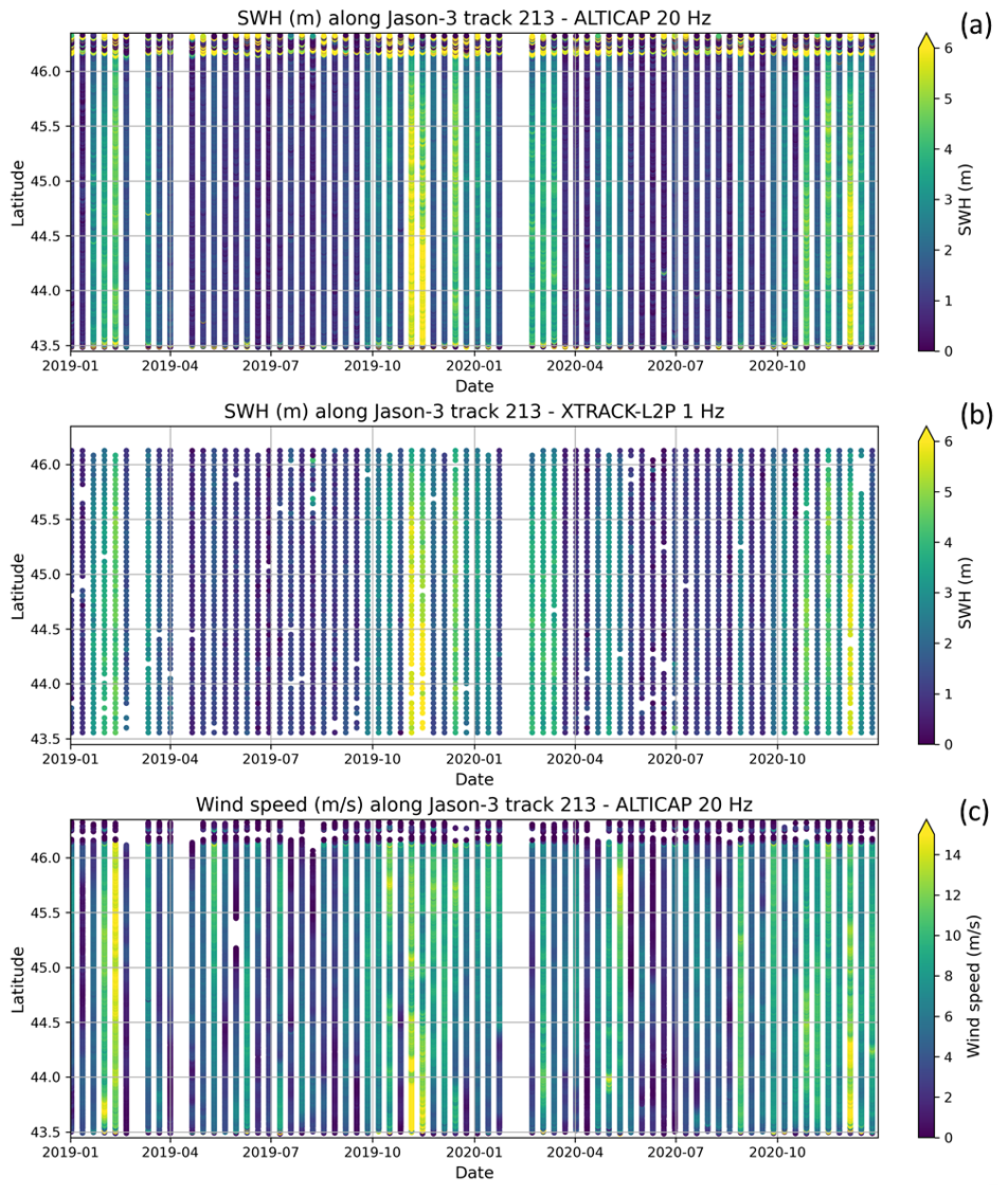
Figure 10 Time-latitude diagrams of the Significant Wave Heights (SWH) from the X-TRACK 1 Hz product (a) and the ALTICAP 20 Hz product (b), and wind speed from the ALTICAP 20 Hz product (c), along the Jason-3 track 213 in the Bay of Biscay, for the time period 2019–2020.

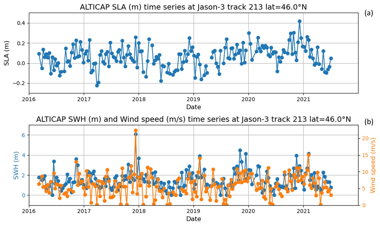
Figure 11 Time series of (a) SLAs and (b) Significant Wave Heights (SWH) and Wind speeds from the ALTICAP 20 Hz product at one point (latitude = 46.0° N) of the Jason-3 track 213 in the Bay of Biscay, for the whole time period available (2016–2021). The SWHs larger than 10 m have been edited for the plot.

4 Product content and distribution

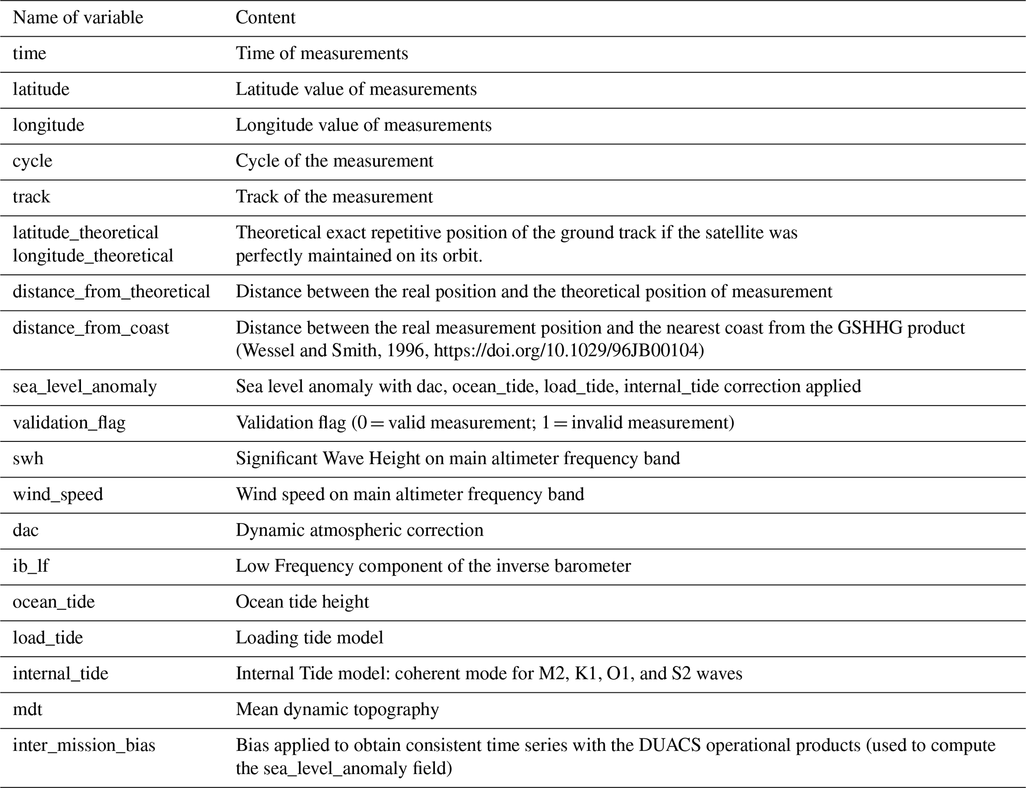
The ALTICAP product is distributed at Level-2P (L2P) altimetry processing level. The L2P products are along track datasets that contain time, point measurement location (longitude and latitude) and SLA, but also information on data validity (validation flag as described in Sect. 3.2) as well as all geophysical parameters and corrections that have been used to compute the SLA. In ALTICAP, it was decided to provide additional geophysical information such as the collocated wind speed and SWH derived from Jason-3 in order to address and facilitate a large number of coastal applications (see Figs. 10 and 11 for example). Information about the theoretical ground track positions (exact repetitive positions that the ground track would have if the satellite was perfectly maintained on its orbit) and the distance to the nearest theoretical repetitive ground track point is also provided to easily build the time series over the whole period from the original along-track data. Finally, ALTICAP contains all the variables described in Table 3, within the global coastal strip between 0 and 500 km offshore.

Table 3 Variables provided in the ALTICAP netcdf files.

The ALTICAP product (https://doi.org/10.24400/527896/a01-2023.020, LEGOS et al., 2023) is available through the ODATIS and AVISO+ services (https://www.odatis-ocean.fr/en/data-and-services/data-access/direct-access-to-the-data-catalogue#/metadata/a3370f6c-5341-42bd-9ba8-0748081c54b3, last access: 26 March 2026). It is distributed in netcdf format. Two different file organizations are proposed, to address a large range of applications:

• per day files containing all the measurements of one day over the globe;

• per track files containing the full time series at each point location along one altimeter track.

Typically, the per day files can be used for comparisons with other daily datasets, or for data assimilation in a numerical model (same format as CMEMS), while the per track files are more suited for local time series analyses and along track statistics. Both datasets contain exactly the same physical information.

Jupyter Notebooks are provided to users alongside the ALTICAP product on the AVISO+ website (https://www.aviso.altimetry.fr/en/data/products/sea-surface-height-products/global/altimetry-innovative-coastal-approach-product-alticap.html, last access: 26 March 2026), with examples of codes to read and plot both types of files. One of the notebooks also gives examples of comparisons with in situ observations, including the computation of cross track geostrophic currents derived from ALTICAP.

5 Data availability

The ALTICAP dataset (https://doi.org/10.24400/527896/a01-2023.020, LEGOS et al., 2023) is publicly available through the ODATIS and AVISO+ services (https://www.odatis-ocean.fr/en/data-and-services/data-access/direct-access-to-the-data-catalogue#/metadata/a3370f6c-5341-42bd-9ba8-0748081c54b3, last access: 26 March 2026).

The following datasets used for this work are publicly available (see the reference list for more details to access):

• all tide gauge observations from the UHSLC (Caldwell et al., 2015) and SHOM (https://data.shom.fr/, last access: 15 October 2021) services;

• GDR altimetry products (https://www.aviso.altimetry.fr/en/data/products/, CNES, 2024a, b);

• X-TRACK altimetry product (https://doi.org/10.24400/527896/A01-2022.020, CTOH, 2023);

• GPD+ wet tropospheric correction (Fernandes et al., 2014);

• EOT20 tidal model (https://doi.org/10.17882/79489, Hart-Davis et al., 2021b);

• FES2014b tidal model (LEGOS et al., 2015);

• FES2022b tidal model (https://doi.org/10.24400/527896/A01-2024.004, LEGOS et al., 2024);

• CNES_CLS22 MSSH (https://doi.org/10.24400/527896/A01-2022.017, CLS, 2022).

Some datasets are not publicly available as they either were specifically processed for the study or will be published in the next altimetry GDR data reprocessing or on the AVISO website (https://www.aviso.altimetry.fr/en/home.html, last access: 15 September 2025). These datasets are:

• ALES range and SSB correction;

• SSB corrections – MLE4 2D and 3D at 20 Hz, Adaptive 2D and 3D at 20 Hz;

• MSS model – SIO;

• tidal models – FES2014b and FES2022b on their native unstructured grids.

Please note that the ALES range and SSB correction are specific products from the ESA CCI Sea Level project, and should not be confused with the SSH/ALES Level-3 datasets produced by DGFI-TUM and distributed via OpenADB (https://openadb.dgfi.tum.de, last access: 26 March 2026).

6 Conclusions and perspectives

The ALTICAP dataset is a new coastal altimetry product that aims to address some of the current gaps in the coastal altimetry datasets that are available today: high resolution posting rate (20 Hz), global coverage of the coastal domain up to 500 km offshore, state of the art and dedicated algorithms, user friendly product in two different formats, providing auxiliary variables and corrections, as well as a validation flag. The construction of the product is based on the objective metrics of a round robin exercise focusing on the coastal ocean (defined here as the region between 0 and 200 km from the coast) and considering six out of 13 SLA components, for a total of 22 algorithms tested. This opportunity was taken to develop specific tools that will be used in the future to analyze and test new algorithms as and when they become available. For example, among the SLA components that were not evaluated during this first round robin exercise, the Dynamic Atmospheric Correction (DAC) is the most likely to contain large uncertainties in coastal regions, due to the high spatial and temporal variability of surge conditions in such areas (Carrère et al., 2016). No alternative solution to the operational correction available in the GDR products (Carrère et al., 2003, LEGOS/CNRS/CLS, 1992) could be considered at the time of this round robin exercise, but some complementary activities are planned in the near future, including the new DAC based on ERA5 reanalysis from ECMWF (CLS and CNRS-LEGOS, 2025).

The ALTICAP product can be used for a large range of coastal applications that include the analysis of the local variability of the coastal sea level and derived geostrophic currents, in connection with the variability observed further offshore, and in synergy with in situ observations (e.g., tide gauges, currentmeters, drifting buoys, high frequency radars …) and other satellite measurements (e.g., sea surface temperature, ocean color, ocean surface rugosity …). It can also be used for the validation of numerical simulations and for data assimilation into models. As collocated SWH and wind speed information is provided alongside the ALTICAP SLAs, as well as auxiliary parameters (tide and DAC corrections in particular), analyses of specific events such as storms can be performed. It is important to note that the performance analysis presented in this data paper is limited to the tide gauge stations that have been selected for the validation, even if they provide a large diversity of situations. The results can differ (in a better or lesser way) depending on the region, the coastline and topography configurations, and the local ocean dynamics. In addition, the ALTICAP product is provided at full resolution (20 Hz) and users will probably need to smooth the along track data to remove the high frequency noise and access the geophysical signals. Depending on the region of interest, the most appropriate smoothing length may differ, hence we let the users choose their own filtering and processing strategies. Jupyter notebooks are provided with the data set and will help use the most appropriate post-processing depending on the study case.

In the near future, we aim to extend the ALTICAP product to include the past Jason-2 mission and the current Sentinel-6-MF mission, in order to build long time series of coastal SLA, SWH and wind speed. One of the objectives of this work is also to provide space agencies and operational developers with analyses and feedback on the state of the art algorithms that are developed in the coastal altimetry domain, to prepare and accompany the development of the next generation of operational products, including the new generation of altimeters, i.e., swath altimetry, with the currently flying SWOT mission, and the future Sentinel-3-NG-topo Copernicus mission.

Appendix A

In this section, we detail the selection of the altimetric algorithms used to build the ALTICAP dataset. For each SLA component, the process, described in Sect. 2.1, consists in an intercomparison of the different altimetric algorithms available, based on their respective overall performance in the coastal domain, considering two different satellite altimetry missions (Jason-2 and Jason-3). For this work, the coastal domain is defined as the coastal strip between the shoreline and the first 200 km offshore. The choice of 200 km is motivated by the need to achieve the best possible product quality across a wide range of spatial scales characterizing coastal processes. For the sake of brevity, we only show a selection of the round robin diagnostics, for the Jason-3 mission. However, all the plots and results of this study are freely available on line on the AVISO+ website (https://www.aviso.altimetry.fr/en/data/products/sea-surface-height-products/global/altimetry-innovative-coastal-approach-product-alticap/roundrobin-reports.html, last access: 26 March 2026).

A1 Altimeter range and Sea State Bias (SSB)

The altimeter range is defined as the distance between the satellite and the instantaneous sea surface directly below the satellite. It is therefore the main measurement of the sea level estimate. In order to obtain a precise range, we must determine the distance between the altimeter and the closest point of the illuminated surface. This is done via a ground processing step called retracking, where an analytical model is fitted to the radar echo, in order to derive the altimeter range.

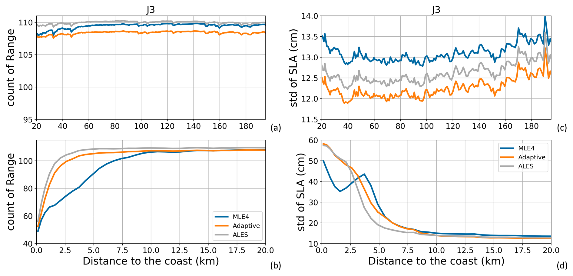
Figure A1 (a, b) Global mean number of valid range data along all Jason-3 tracks for the period 17 February 2016 to 22 February 2019 (111 cycles). (c, d) Global mean of standard deviation values (in cm) of the SLA along all Jason-3 tracks for the same period, when using the different range solutions. Results are presented as a function of the distance to the coast (in km) between 200 and 20 km (a, c) and between 20 and 0 km (b, d) from the coast.

The amplitude and propagation direction of ocean waves relative to the satellite's trajectory impact the altimetric measurement, generating biases in the range estimation. The SSB correction aims to minimize this effect. This correction is computed using outputs from the retracking, such as the significant wave height (SWH) and the surface wind speed. Given that both the range and the SSB are derived from the same analytical model, they are codependent in the SLA calculation

The SSB solutions that exist today can be classified as either 2D or 3D, depending on the number of input parameters used in the computation. While the 2D solution is based on the SWH and surface wind speed (Melville et al., 2004), the 3D solution also includes the mean wave period derived from a wave model (Tran et al., 2010).

Three retracking solutions were compared within this round-robin exercise: MLE4 (Thibaut et al., 2010), ALES (Passaro et al., 2014) and Adaptive (Poisson et al., 2018). The analyses were done for the range specifically, and for the following SSB solutions. Only Jason-3 data were used here as some of these SSB solutions were not available for Jason-2 at the time of the round robin exercise:

• MLE4 retracking: SSB 2D at 1 Hz (GDR standard) interpolated at 20 Hz, SSB 2D directly computed at 20 Hz, SSB 3D at 20 Hz

• ALES retracking: SSB 2D at 20 Hz

• adaptive retracking: SSB 2D at 20 Hz, SSB 3D at 20 Hz.

As we can see in Fig. A1, the three range solutions tested perform differently in the coastal region, and the results are also mission-dependent. In particular, for the MLE4 range, an important data loss between the coast and 20 km offshore can be noted in the Jason-3 data (Fig. A1a and b), which is not visible in the Jason-2 data (not shown here, but all Jason-2 results are available online on the AVISO+ website). The drop in the MLE4 range availability translates into an artificial decrease in the coastal variability of the SLA computed with this retracking solution (Fig. A1d). On the other hand, ALES and the Adaptive retracker solutions show similar valid data counts, with still more than 80 cycles of valid data on average (out of the 111 cycles tested) in the last kilometer before the shore (Fig. A1b). Between 2.5 and 10 km to the coast, the ALES solution performs better than the Adaptive solution, with lower variability in the SLA. Between the coast and 2.5 km, both solutions perform similarly (Fig. A1d). However, in the more open-ocean region (between 20 and 200 km offshore), the SLA based on the ALES solution shows about 0.5 cm more variability than the Adaptive solution (Fig. A1c).

Regarding the SSB, Passaro et al. (2018) showed that the computation of the SSB correction directly at 20 Hz improves the accuracy of the SLA estimate. Moreover, according to Tran et al. (2021), using a 3D version of the SSB correction instead of the standard 2D version results in an SLA variance reduction for the high-frequency signals. Here, the results are mitigated by the availability of some of the SSB corrections in our working database, in particular for the SSB Adaptive 3D that shows a large decrease in availability from about 100 km offshore to the coast, due to the resolution of the wave model in this region (Fig. A2a and b). Still, one can clearly note the better performance with the MLE4 SSB 3D compared to the MLE4 SSB 2D, and with the Adaptive SSB 3D compared to the Adaptive SSB 2D, as the 3D approach systematically provides lower variability in the SLA, whatever the distance to the coast (Fig. A2c and d). As for the range, the ALES SSB shows very good performance in the most coastal region, between 0 and 10 km offshore. However, it results in more variability than most other solutions in the more open-ocean SLA estimates.

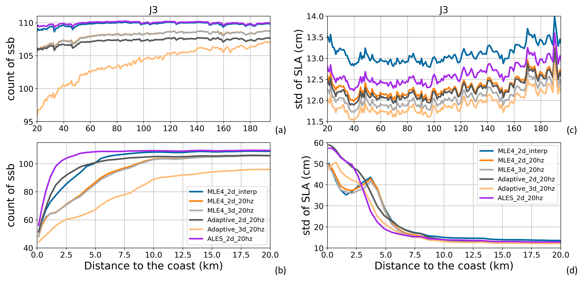
Figure A2 (a, b) Global mean number of valid SSB data along all Jason-3 tracks for the period 17 February 2016 to 22 February 2019 (111 cycles). (c, d) Global mean of standard deviation values (in cm) of the SLA along all Jason-3 tracks for the same period, when using the different SSB solutions. Results are presented as a function of the distance to the coast (in km) between 200 and 20 km (a, c) and between 20 and 0 km (b, d) from the coast.

These results, as well as the availability of the Adaptive retracking algorithm (range and SSB 3D) for Jason-2 and Jason-3, have driven our choice for implementation in the ALTICAP product, over the ALES solution. Concerning the SSB, the data availability issue of the Adaptive SSB 3D in our database was corrected and it could thus be chosen for ALTICAP.

A2 Ionospheric correction

As the radar wave travels through the ionosphere, it interacts with the free electrons that are present there. This translates into a delay in the radar signal propagation that must be taken into account in order to accurately determine the distance between the altimeter and the sea surface; it is called ionospheric correction.

During the round robin selection process, two solutions were evaluated. The first one corresponds to the filtered version of the satellite altimetry dual-frequency linear combination (Chelton et al., 2001). The second method uses external data provided by GNSS based ionosphere estimates (Komjathy and Born, 1999), the GIM (Global Ionospheric Map) solution. This solution is mostly implemented for single frequency altimeters, as the dual frequency filtered method becomes impossible to apply.

When comparing the ionospheric correction counts for Jason-2 (not shown here, but available online on the AVISO+ website) and Jason-3, a drop is noticeable in the Jason-3 filtered dual frequency correction when approaching the coast, with the loss of about 18 % of the cycles (20 cycles out of 111) in the last 10 km (Fig. A3a and b). This is due to a processing issue that is under investigation by the data producer. This loss of data results in an artificial decrease in the variability of the SLA estimates, compared to the GIM solution (Fig. A3c and d). Indeed, for Jason-2, the comparison between GIM and the filtered dual frequency corrections shows very close performance in the coastal region, with a slightly lower dispersion for the dual-frequency correction. To avoid losing data due to the ionosphere correction availability in the coastal region, we thus chose to use the GIM correction in the ALTICAP dataset.

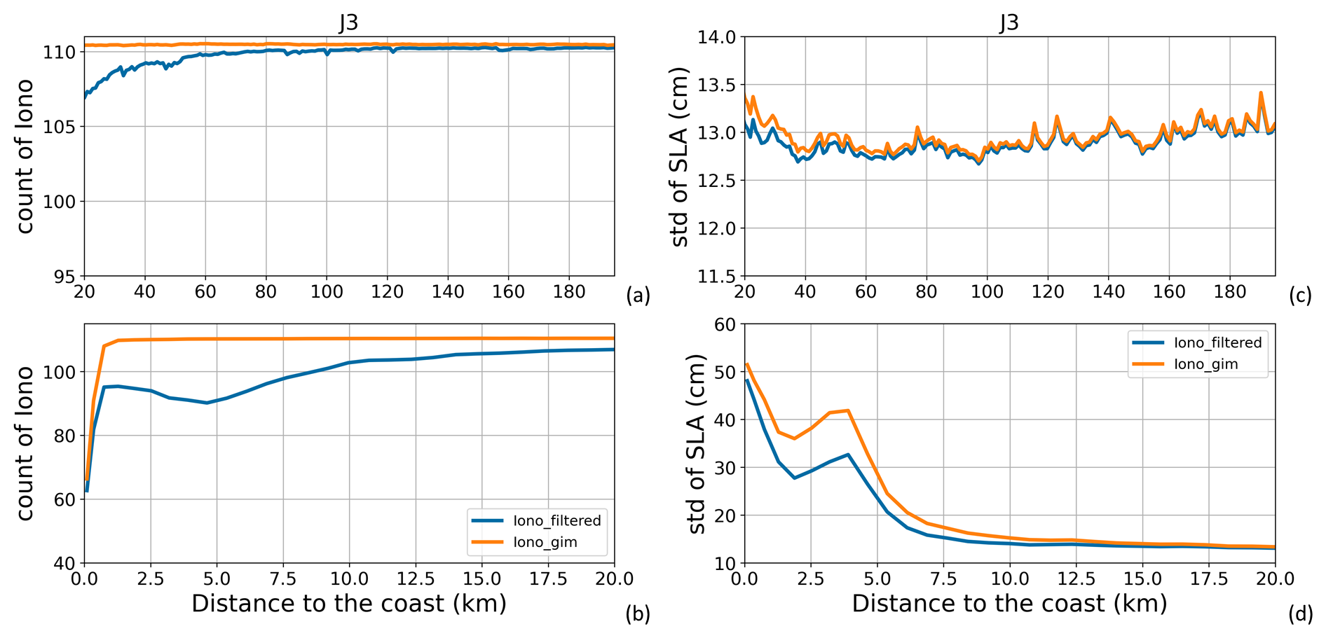
Figure A3 (a, b) Global mean number of valid ionospheric correction data along all Jason-3 tracks for the period 17 February 2016 to 22 February 2019 (111 cycles). (c, d) Global mean of standard deviation values (in cm) of the SLA along all Jason-3 tracks for the same period, when using the different ionospheric correction solutions. Results are presented as a function of the distance to the coast (in km) between 200 and 20 km (a, c) and between 20 and 0 km (b, d) from the coast.

A3 Wet tropospheric correction

As for the ionospheric correction, the radar signal experiences a path delay in the lower atmosphere, this time due to the liquid water and vapor. Here again, we need a specific correction called the Wet Tropospheric Correction. It is generally computed either from direct onboard radiometer measurements or from external meteorological models. The first solution is more accurate but in the coastal zone, the signal coming from the surrounding land contaminates the radiometer measurements, resulting in significant errors (Lázaro et al., 2020) A solution proposed to tackle this, and also to improve the wet-troposphere estimates over the coastal area is the so called GPD+ (GNSS derived Path Delay) solution (Fernandes et al., 2015) that combines information from several sources to build an objective-analysis estimate of the wet-troposphere component.

In order to determine the appropriate correction to be used in the ALTICAP product, we compared the results obtained with three different solutions: the radiometer-derived correction, the correction computed from the ECMWF model and the GPD+ correction.

Over the open ocean, the behavior of the three solutions is very similar and stable both in terms of valid data count (Fig. A4a) and standard deviation of the SLA (Fig. A4c). In the very coastal domain (less than 2.5 km from the coast), the valid data count drops for the three solutions (slightly earlier for the GPD+ solution than the two others). In terms of SLA variability, the three corrections also provide very close results in the coastal domain (Fig. A4d). When plotting the differences with the radiometer reference solution (Fig. A4e), the GPD+ solution performs slightly better than direct radiometric measurements and the ECMWF model estimates in the first 10 km offshore (about 0.5 cm less variability). Based on these analyses, the GPD+ solution was chosen to be implemented in the ALTICAP product.

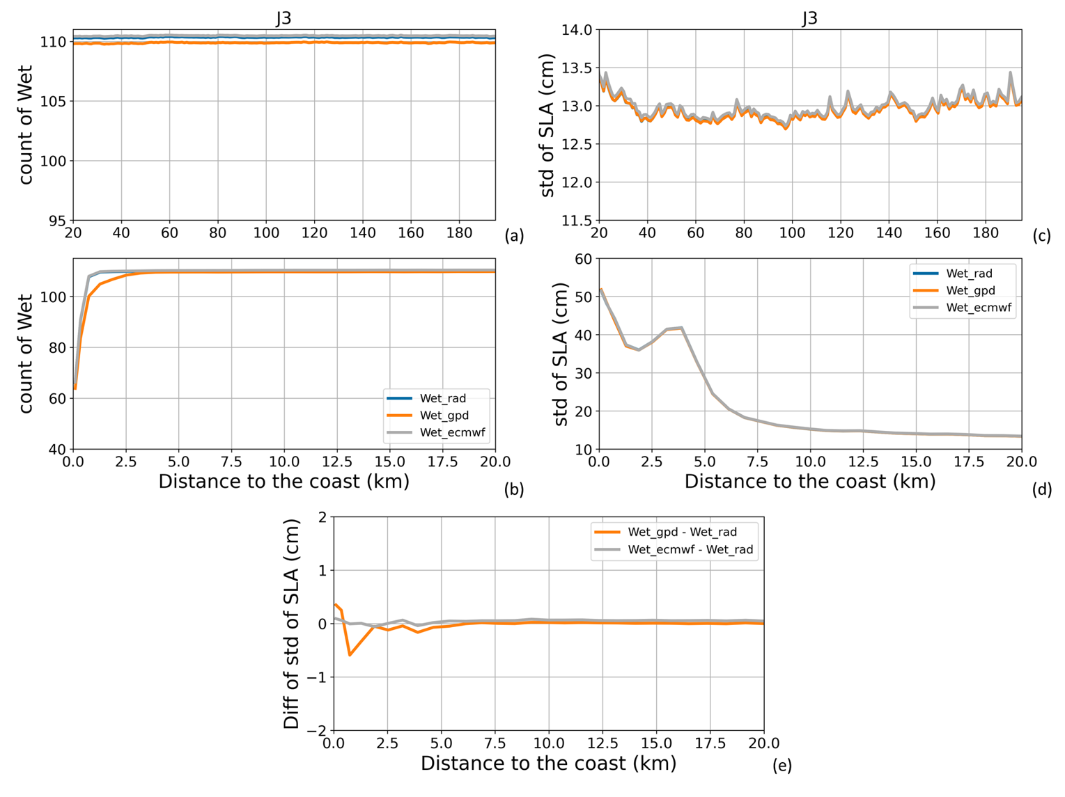
Figure A4 (a, b) Global mean number of valid wet tropospheric correction data along all Jason-3 tracks for the period 17 February 2016 to 22 February 2019 (111 cycles). (c, d) Global mean of standard deviation values (in cm) of the SLA along all Jason-3 tracks for the same period, when using the different wet tropospheric correction solutions. (e) Difference (in cm) between the global mean of standard deviation values of the SLA along all Jason-3 tracks for the same period, when using the different wet tropospheric solutions and when using the reference solution (radiometer). Results are presented as a function of the distance to the coast (in km) between 200 and 20 km (a, c) and between 20 and 0 km (b–e) from the coast.

A4 Ocean tide correction

The tidal signal is under sampled by the orbital period of the satellite altimeters (10 d or more, depending of the mission), leading to frequency aliasing in the altimeter sea level estimates. The problem is tackled by using a global ocean tide model to remove the ocean tide elevation from the altimeter sea level. Over the open ocean, recent ocean tide models exhibit an error level contained below 2 cm RMS (Stammer et al., 2014; Zaron and Elipot, 2020), which can be considered as part of the lower tier in the global error budget. However, in shallow coastal waters, the global tidal models are less precise, with errors that can reach 15 cm RMS. It is explained by the complex hydrodynamic characteristics of the coastal domain coupled with imperfect knowledge of the bathymetry, which makes difficult accurate modelling of coastal ocean tides.

Three tide models were investigated for implementation in ALTICAP: the EOT20 model (Hart-Davis et al., 2021b), the FES2014b model (Lyard et al., 2021) and the FES2022b model (Carrère et al., 2022). The FES2014b model was tested under its released version, interpolated on a 1/16° regular grid, and also with its native unstructured grid (resolution ranging from ∼4 to 15 km in the coastal region), in order to investigate the impact of the loss of resolution due to the change of grid in the coastal domain. It results in four solutions for this SLA component.

Over the open ocean, the impact of all algorithms is very similar both in terms of valid data count (Fig. A5a) and standard deviation of the SLA (Fig. A5c). In the very coastal domain, less than 2.5 km from the coast, the valid data count drops for all the solutions (Fig. A5b). The drop occurs slightly earlier for the FES2014b unstructured solution than for the others, probably because the latter are all on regular grids with some extrapolation to cover the whole ocean. In terms of SLA variability, EOT20 is systematically a few millimeters above all the other solutions except in the most coastal 7 km (Fig. A5c–e). This may be due to the fact that the EOT20 tidal spectrum contains less components than the others, thus removing less tidal signal from the altimetry SLA data. Indeed, 17 tidal components are available in EOT20 but only 15 of them could be used for this study for reasons of incompatibility with the dynamic atmospheric correction (Hart-Davis et al., 2021a), while 34 tidal components were used for FES2014b and FES2022b. The largest differences in terms of SLA standard deviation occur between the structured and unstructured versions of FES2014b, in the last 5 km (Fig. A5e). This is clearly the impact of the smoothing that happens when interpolating from the unstructured grid to the regular grid at 1/16° (i.e., about 7.5 km). The FES2022b new model on the regular grid (1/30° resolution, i.e., about 4 km) clearly provides lower SLA variability than FES2014b on regular grid, between 0 and 15 km offshore. In order to fully benefit from the resolution of the FES2022b, the FES2022b unstructured solution was used to build the ALTICAP dataset.

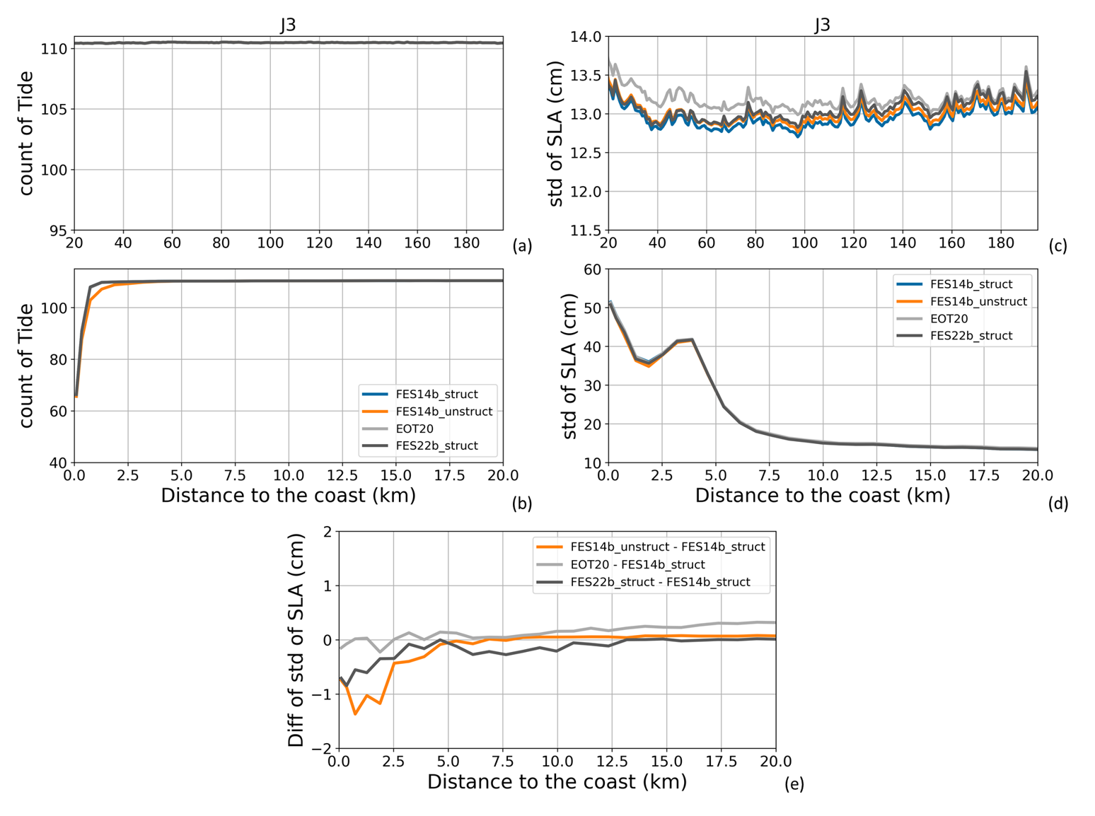
Figure A5 (a, b) Global mean number of valid ocean tide correction data along all Jason-3 tracks for the period 17 February 2016 to 22 February 2019 (111 cycles). (c, d) Global mean of standard deviation values (in cm) of the SLA along all Jason-3 tracks for the same period, when using the different ocean tide correction solutions. (e) Difference (in cm) between the global mean of standard deviation values of the SLA along all Jason-3 tracks for the same period, when using the different tide solutions and when using the reference solution (FES2014b struct). Results are presented as a function of the distance to the coast (in km) between 200 and 20 km (a, c) and between 20 and 0 km (b–e) from the coast.

A5 Mean Sea Surface Height (MSSH)

In order to obtain the variable component of the sea surface height, the average or steady state component, the MSSH must also be computed and removed from the altimeter sea level estimate. In current altimetry processing, the MSSH is obtained by time averaging and interpolating the instantaneous sea surface height data observed by the different altimeters over a finite period, over a regular grid that covers the world ocean. Given inhomogeneities in the spatial sampling of altimetry, regional errors, and changes in measurement technology, the MSSH estimates evolve every few years, improving on the last iteration. Over the open ocean, the errors associated with this term are in the order of 1–2 cm² RMS (Pujol et al., 2018) and increase over the coastal domain.

The MSSH products considered in the round robin are the CNES_CLS15 dataset (Pujol et al., 2018), the SIO dataset (Sandwell et al., 2017) and the CNES_CLS22 dataset computed over a 29 year period (1993–2021) (Schaeffer et al., 2023), which was the latest version produced by CNES at the time of the study. Compared to the previous iteration (CNES_CLS15), the CNES_CLS22 MSSH better accounts for the interannual and seasonal ocean variations, and significantly improves the coverage of the Polar oceans. In the coastal area, it shows an improvement of 6 % of variance reduction in the first 5 km from the coast with respect to the previous version (Schaeffer et al., 2023).

The round-robin diagnostics (Fig. A6) show that the three MSSH solutions are nearly identical over the ocean, with an almost indistinguishable dispersion, as we compare on the historical Jason track, where the MSSH are generally all well constrained. Differences arise over the coastal band, in the last 20 km (Fig. A6e). There, the SIO MSSH shows larger variability than the reference solution (CNES_CLS15). On the other hand, the CNES_CLS22 solution provides slightly lower SLA variability than CNES_CLS15. The CNES_CLS22 MSSH solution was chosen to be implemented in the ALTICAP dataset.

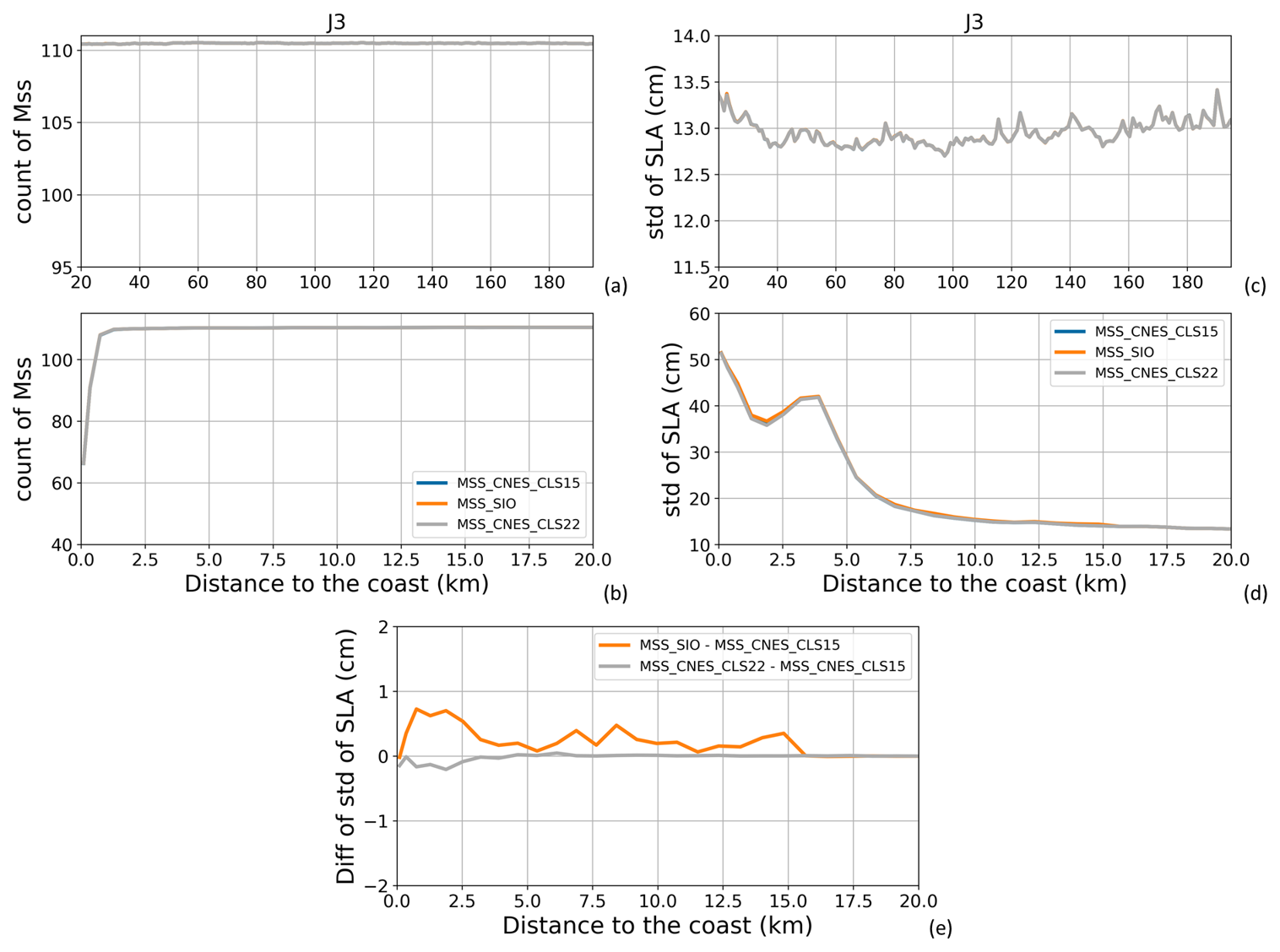
Figure A6 (a, b) Global mean number of valid MSSH data along all Jason-3 tracks for the period 17 February 2016 to 22 February 2019 (111 cycles). (c, d) Global mean of standard deviation values (in cm) of the SLA along all Jason-3 tracks for the same period, when using the different MSSH solutions. (e) Difference (in cm) between the global mean of standard deviation values of the SLA along all Jason-3 tracks for the same period, when using the different MSSH solutions and when using the reference solution (CNES-CLS15). Results are presented as a function of the distance to the coast (in km) between 200 and 20 km (a, c) and between 20 and 0 km (b–e) from the coast.

Appendix B

In this section, we provide maps of the comparison between the tide gauge in situ observations and the ALTICAP edited 20 Hz dataset and the X-TRACK 1 Hz dataset. Figure B1 shows the correlation between tide gauge and altimetry SLAs for each tide gauge station. The altimetry points are selected so as they are located less than 20 km from the coast and less than 50 km from the tide gauge station.

The selected tide gauges present a large diversity of configurations, with relatively straight coastlines (e.g., Esperance, Sète, La Réunion and Ponta Delgada) or very indented coastlines (e.g., Newport and Tofino). In some cases, the tide gauge is located in a harbor (e.g., Galveston, Newport, Mar del Plata, Maisaka, Dakar) or in an estuary (e.g., Visakhapatnam) and may thus see rather different dynamics than the altimetry track on the open ocean. Sometimes, there is an island or an island chain between the tide gauge and the altimetry track (e.g., Galveston, Newport, Hanimaadhoo, Tofino, Lombrum), and the ocean dynamics may be very different on each side of the island. However, no generic conclusions can be drawn for each type of configuration, as the results are very contrasted and strongly depend on the main drivers of the local ocean dynamics. For example, although the Galveston tide gauge is located in a harbor, in a narrow channel, and behind an island, the correlations with altimetry are very high (>0.8) because the main process in the region (Gulf of Mexico) is the steric effect. Lower correlations at some other places can be explain by very local dynamics, once the tides and wind and atmospheric pressure effects are removed from the SLAs in the observations.

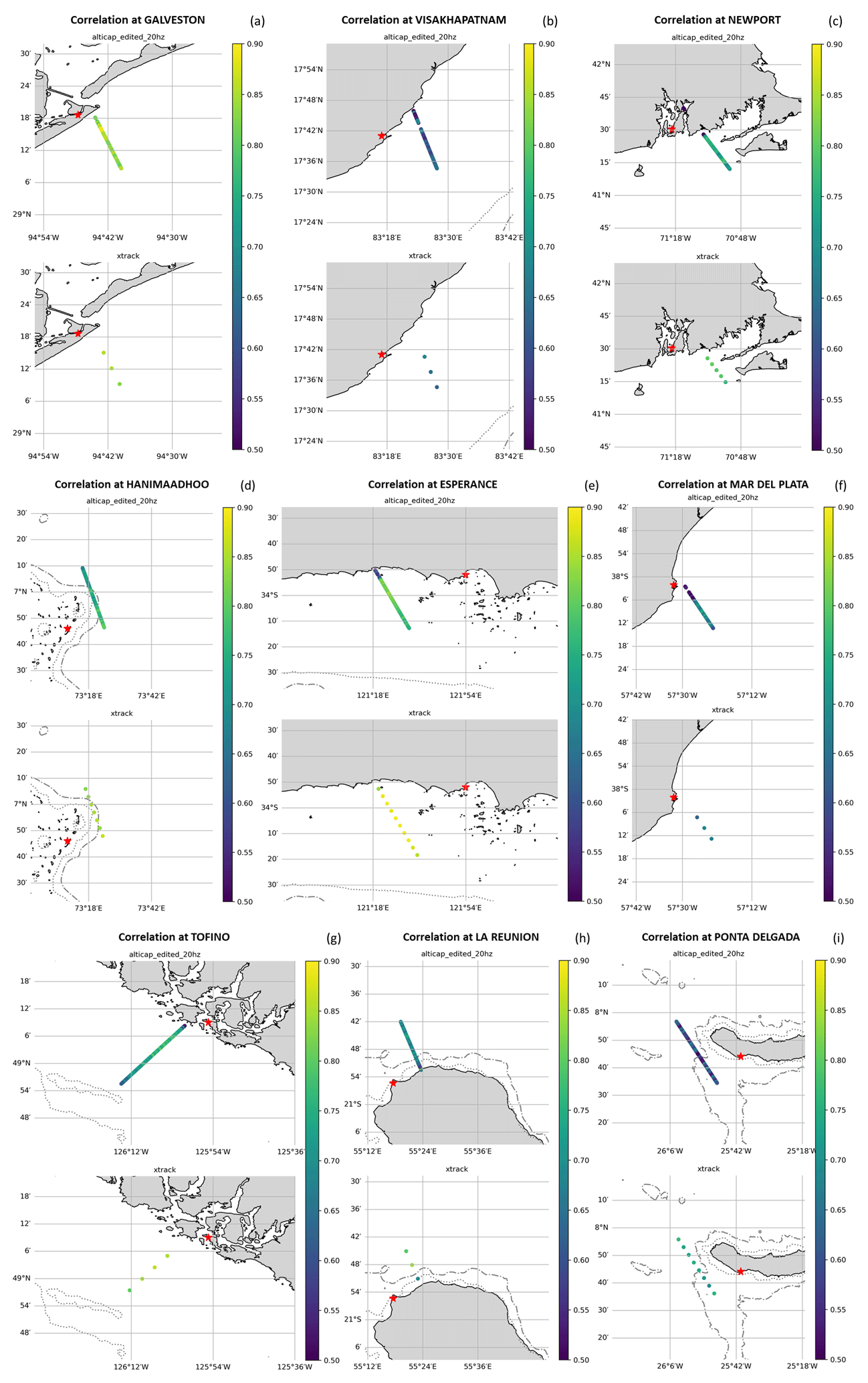
Figure B1 (a–n) Maps of the correlation between each of the 14 tide gauge stations (red star on each map) and the along track altimetry SLAs (dots in color) from the ALTICAP 20 Hz dataset (upper plots) and the X-TRACK 1 Hz dataset (lower plots). Only altimetry points located at a distance lower than 20 km from the coast and 50 km from the tide gauge station are considered. The dot and dash-dot lines show the 200 and 1000 m isobaths respectively.