Australia's terrestrial industrial footprint and ecological intactness

Australia's unique biodiversity faces significant threats from anthropogenic activities that drive habitat destruction and degradation. This study presents the first comprehensive national-scale cumulative pressure map for terrestrial Australia since the 1980s, providing key insights into human disturbance of the landscape. We developed a Human Industrial Footprint (HIF) index map at a 100 m spatial resolution, incorporating 16 nationally relevant pressure layers, which offers a contemporary assessment of cumulative pressures on Australia's landscapes. The HIF was used to derive an Ecological Intactness Index (EII), which accounts for habitat loss, quality, and fragmentation, to provide an estimate of an area's structural intactness. A technical validation comparing visually scored pressures in 1397 stratified random samples using high-resolution satellite images revealed a strong agreement with the mapped pressure values (the HIF). We also conducted an uncertainty (sensitivity) analysis by adjusting individual pressure scores by up to ±50 % across 100 000 simulations, which showed a moderate impact on cumulative pressure scores, confirming the robustness of our approach. We believe both the HIF and EII datasets can be valuable tools for guiding conservation efforts, such as informing protected area expansion, ecosystem restoration priorities, and biodiversity offset strategies. By offering a detailed assessment of cumulative pressures and ecological integrity, this study addresses a critical knowledge gap, and can support evidence-based decision-making for Australia's biodiversity conservation and sustainable development objectives. The HIF, EII, and scaled pressure layers are available at https://doi.org/10.5281/zenodo.17606284 (Venegas-Li et al., 2025).

1 Introduction

Australia is globally recognized as one of the most biodiverse countries on Earth, hosting an array of species and ecosystems found nowhere else (Chapman, 2009). However, since European colonization, industrial activities such as agriculture, forestry, and urbanization have caused widespread habitat destruction, fragmentation, and pollution of the natural environment. As a result, during the last 200 years, one-third of native vegetation has been lost (Bradshaw, 2012; Kingsford et al., 2009; Ward et al., 2019). Over 2100 species and 100 ecological communities are now legislated as threatened with extinction in the near term, and 103 species have become extinct (Commonwealth of Australia, 2025). The threatening processes driving these declines remain largely unabated (Kearney et al., 2023; Legge et al., 2023; Woinarski et al., 2015), and understanding how their extent and intensity interact with natural systems is key to informing conservation policy (Kearney et al., 2019).

The field of cumulative pressure mapping, in which data on multiple pressures are integrated under a spatial model (maps), has become a widely used approach to estimate human pressures on the environment (Watson et al., 2023b). Here, we use the term “pressure” to denote human activities with the potential to harm nature (Borja et al., 2006; Martins et al., 2012), broadly corresponding to “direct threats” or “stressors” in the IUCN Threat and Stress Classification Scheme (Salafsky et al., 2008, 2025). Such pressure maps are increasingly used as proxies for human influence on ecological state and condition, particularly within pressure-state-response frameworks used to guide adaptive planning and management (Watson and Venter, 2019). The conceptual foundations of cumulative pressure maps emerged in the 1980s (Lesslie and Taylor, 1983, 1985; McCloskey and Spalding, 1989), but the discipline has expanded rapidly over the past two decades, with advances in Earth observation and geographic information systems (Watson et al., 2023b; Watson and Venter, 2019). The Human Footprint of Sanderson et al. (2002) is arguably one of the most influential early global assessments of humanity's influence on the terrestrial planet, and mapped at a 1 km resolution, provided a framework to quantify anthropogenic influence across nine major pressures. This framework has since been refined and adapted to incorporate additional pressures (Kennedy et al., 2019; Venter et al., 2016a), regional contexts (González-Abraham et al., 2015; Hirsh-Pearson et al., 2022; Martinuzzi et al., 2021; Theobald, 2013; Woolmer et al., 2008), and alternative models for aggregating pressures (Halpern et al., 2008; Theobald, 2013), while recent efforts have achieved spatial resolutions of 100–300 m and annual updates (Gassert et al., 2023; Mu et al., 2022; Theobald et al., 2025). Comparable methods have also been applied in marine systems to quantify the extent and intensity of human use of the oceans (Ban et al., 2010; Halpern et al., 2008, 2015; Micheli et al., 2013).

Cumulative pressure maps are understood to represent potential human influence rather than the realised ecological state or condition of natural systems (Theobald et al., 2025; Venter et al., 2016b). Nonetheless, they have become foundational datasets for ecological research, conservation planning, and environmental reporting, where higher pressures correspond to degraded or lower ecological integrity areas, and lower pressures to areas closer to their natural state. For example, these maps have been used to evaluate relationships between human pressures and species extinction risk (Di Marco et al., 2018; Ramírez-Delgado et al., 2022; Torres-Romero et al., 2025), analyse changes in global mammal distributions (Tucker et al., 2021), population level changes in great apes' behaviour and densities (Kühl et al., 2019; Ordaz-Németh et al., 2021), as well as model the spread of infectious diseases (Skinner et al., 2023). Moreover, cumulative pressure maps have been used in major environmental assessments, including the IPBES Global Assessment (IPBES, 2019), the Intergovernmental Panel on Climate Change (IPCC) reports (Masson-Delmotte et al., 2018), and the latest Global Biodiversity Outlook (Secretariat of the Convention on Biological Diversity, 2020), where they have directly informed indicators of human impact and ecosystem condition.

Pressure maps have been used as surrogates for ecological intactness. However, intactness (often used as a synonym for areas of high integrity) describes the degree to which systems retain their natural composition, structure, and function (Nicholson et al., 2021). Pressure maps may therefore not fully capture intactness, as they do not account for the spatial configuration and habitat-quality context surrounding each pixel (Theobald et al., 2025). To overcome this, Beyer et al. (2020) developed a metric to estimate ecological intactness, which integrates relative habitat quality with the degree of fragmentation, using cumulative pressure maps as the base layer. This approach provides a spatially explicit measure of the structural dimension of integrity, complementing cumulative pressure maps that represent direct human influence. Developing intactness metric datasets is particularly important in the context of the global conservation agenda (Mendez Angarita et al., 2025) because targets have been set for retaining ecological intactness in the Kunming-Montreal Global Biodiversity Framework (GBF) (CBD, 2022), to which Australia is a signatory and has made commitments to. Specifically, the ecosystem component of the GBF's Goal A aims to ensure “the integrity, connectivity, and resilience of all ecosystems are maintained, enhanced, or restored, substantially increasing the area of natural ecosystems by 2050”. This is to be achieved through activities including protection and restoration (Targets 1–3) (CBD, 2022).

In Australia, Lesslie et al. (1988) and Lesslie and Taylor (1983, 1985) carried out pioneering work in the 1980s to create the first pressure map at a national scale. However, no similar efforts have been carried out subsequently for the country, making the available national data highly dated. Global efforts have mapped pressures across Australia, but some of these use a limited set of globally available datasets to represent pressures (Gassert et al., 2023; Mu et al., 2022; Sanderson et al., 2002; Williams et al., 2020) and therefore miss nation-specific critical pressures (Hirsh-Pearson et al., 2022). Others, such as Theobald et al. (2020, 2025), incorporate additional pressures and finer spatial resolution, which likely improves their representation of human influence across many landscapes (Arias-Patino et al., 2024). However, these models may remain constrained by the need to use globally consistent datasets, which might fail to represent features such as rural roads, farm dams, and small-scale mining that are sometimes better mapped within national boundaries. National-scale assessments can overcome some of the limitations of global models by integrating detailed, locally curated datasets derived from bottom-up data collection and long-term government monitoring programs (González-Abraham et al., 2015; Hirsh-Pearson et al., 2022; Martinuzzi et al., 2021; Theobald, 2013; Woolmer et al., 2008). Such datasets are subject to national quality standards and aligned with official land-use reporting frameworks, thereby improving policy relevance (Martinuzzi et al., 2021; Scott and Rajabifard, 2017).

This study aims to produce two complementary national datasets representing cumulative industrial pressures and intactness in Australia around 2022 (based on the median year of the input datasets): the Australian Human Industrial Footprint (HIF) and the Ecological Intactness Index (EII). The HIF is a cumulative pressure map at 100 m spatial resolution that integrates 16 nationally significant pressures, while the EII translates these pressures into an ecologically interpretable measure of structural intactness, following the metric proposed by Beyer et al. (2020). Together, the HIF and the EII offer critical tools for guiding conservation and restoration efforts, aligning with Australia's commitments under the Global Biodiversity Framework, including those targeting highly intact ecosystems (Target 1), where to undertake restoration (T2) where the important areas to protect are (T3), and government objectives and policies such as the Threatened Species Action Plan (Commonwealth of Australia, 2022).

2 Methods

2.1 Overview of the Human Industrial Index Mapping Method

We adapted the Human Footprint Index methodological approach (Sanderson et al., 2002) to create a cumulative pressure map for Australia, incorporating best practices from studies that have refined this method globally and regionally over the past two decades (e.g.; Arias-Patino et al., 2024; Gassert et al., 2023; Hirsh-Pearson et al., 2022; Watson et al., 2023a; Woolmer et al., 2008). Each mapped pressure aligns with one or more IUCN-CMP threat classes (Salafsky et al., 2025, see Table S1 in the Supplement), ensuring conceptual consistency with global biodiversity reporting frameworks (e.g., GBF). This alignment helps guide the selection of pressures to include, clarifies relationships between them, and informs the choice of appropriate datasets and schemes.

We selected pressures based on (i) national data availability at suitable spatial and thematic resolution, (ii) relevance to natural systems as identified in previous footprint frameworks. Consistent with earlier human footprint assessments, we focused on observable industrial pressures, those directly resulting from human activities such as infrastructure, extraction, and land use. Pressures such as pollution, invasive species, climate change, and fire were excluded because suitable national spatial data were unavailable. Climate change and changed fire regimes present additional challenges in distinguishing natural from human-induced events (Bowman et al., 2020; Theobald et al., 2025). Nevertheless, we acknowledge that changes in fire regimes increasingly threaten Australian biodiversity (Doherty et al., 2024; Ward et al., 2020). The framework we use remains flexible, allowing future integration of new pressures (such as changed fire regimes) as suitable datasets become available.

We identified 16 human pressures relevant to Australia with available spatial data (Table 1): (1) intensive land uses, (2) buildings, (3) mining and quarrying, (4) human population density, (5) croplands, (6) pasturelands, (7) forestry plantations, (8) reservoirs and dams, (9) farm dams, (10) roads, (11) railways, (12) hiking trails, (13) oil pipelines, (14) gas pipelines, (15) energy transmission lines, and (16) navigable waterways. We assigned a score between 0 and 10 to each pressure, with each pressure's score relative to other pressures (Fig. 1 and Table S2). For all the pressures, scores were assigned according to their “direct” disturbance on the area they overlap. For pressures 8–16, we also assigned a score to adjacent areas to reflect indirect disturbances, such as edge effects, habitat fragmentation, and more cryptic forms of disturbance, such as potential access for humans or invasive species to areas previously inaccessible. We largely followed past human footprint studies to assign pressure scores to ensure comparability with these (Hirsh-Pearson et al., 2022; Sanderson et al., 2002; Venter et al., 2016b; Woolmer et al., 2008). Several pressure scores were refined through discussions within our author team, which includes researchers with extensive experience in Australian ecosystems and land-use and pressure mapping, to better reflect national conditions and data characteristics. While this approach provided context-specific refinements, future national applications could further strengthen the scoring scheme through structured decision-science methods (e.g., via Delphi methods).

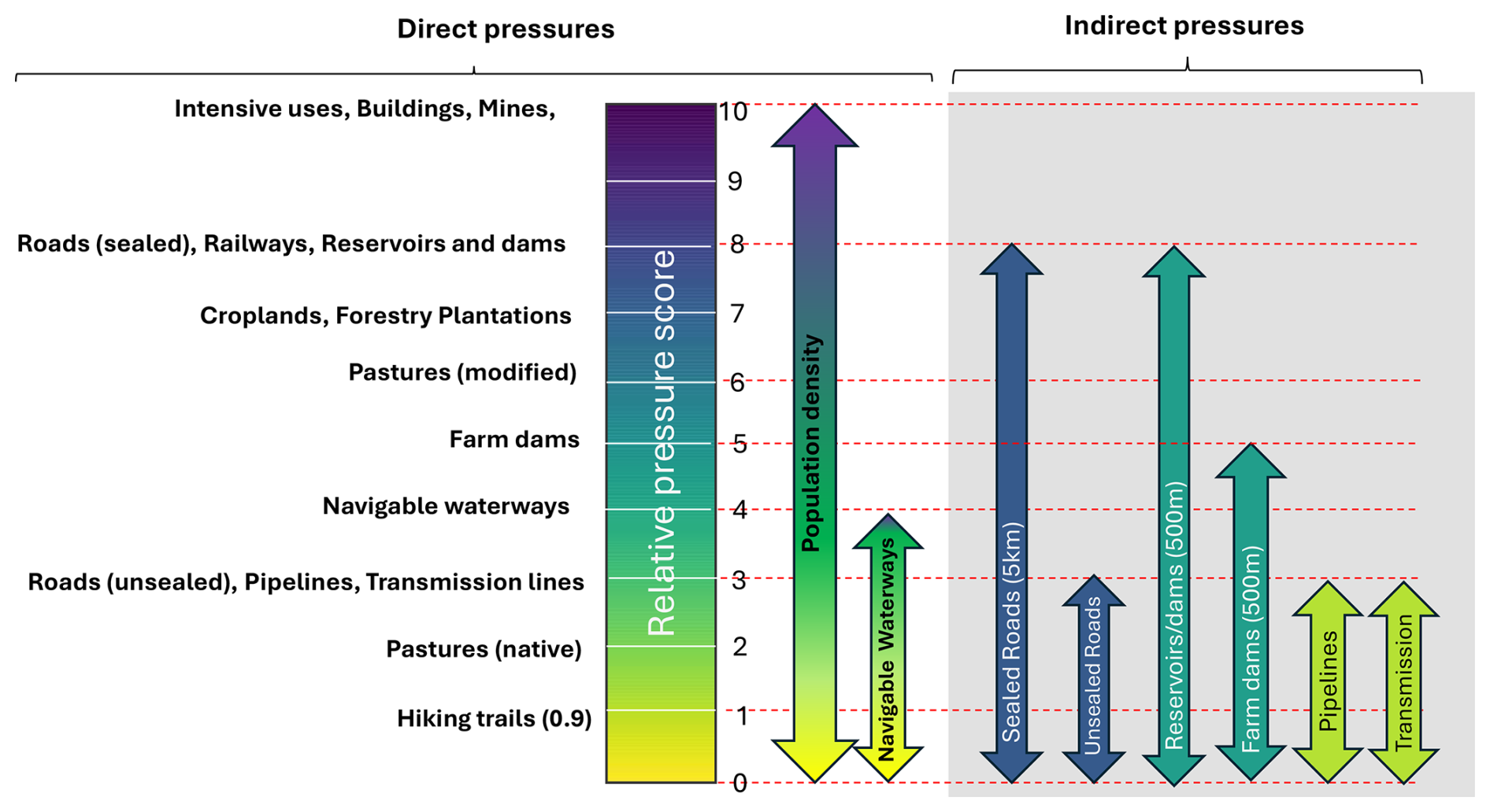
Figure 1 Direct and indirect scores assigned to each of the 16 pressures used to estimate the Australian Industrial Footprint. We set indirect effects to extend 5 km from roads, 500 m from reservoirs and dams, and 2.75 km from pipelines and transmission lines.

Table 1 The pressures included in mapping the Australian Industrial Footprint, and the specific data layers utilised in the mapping process.

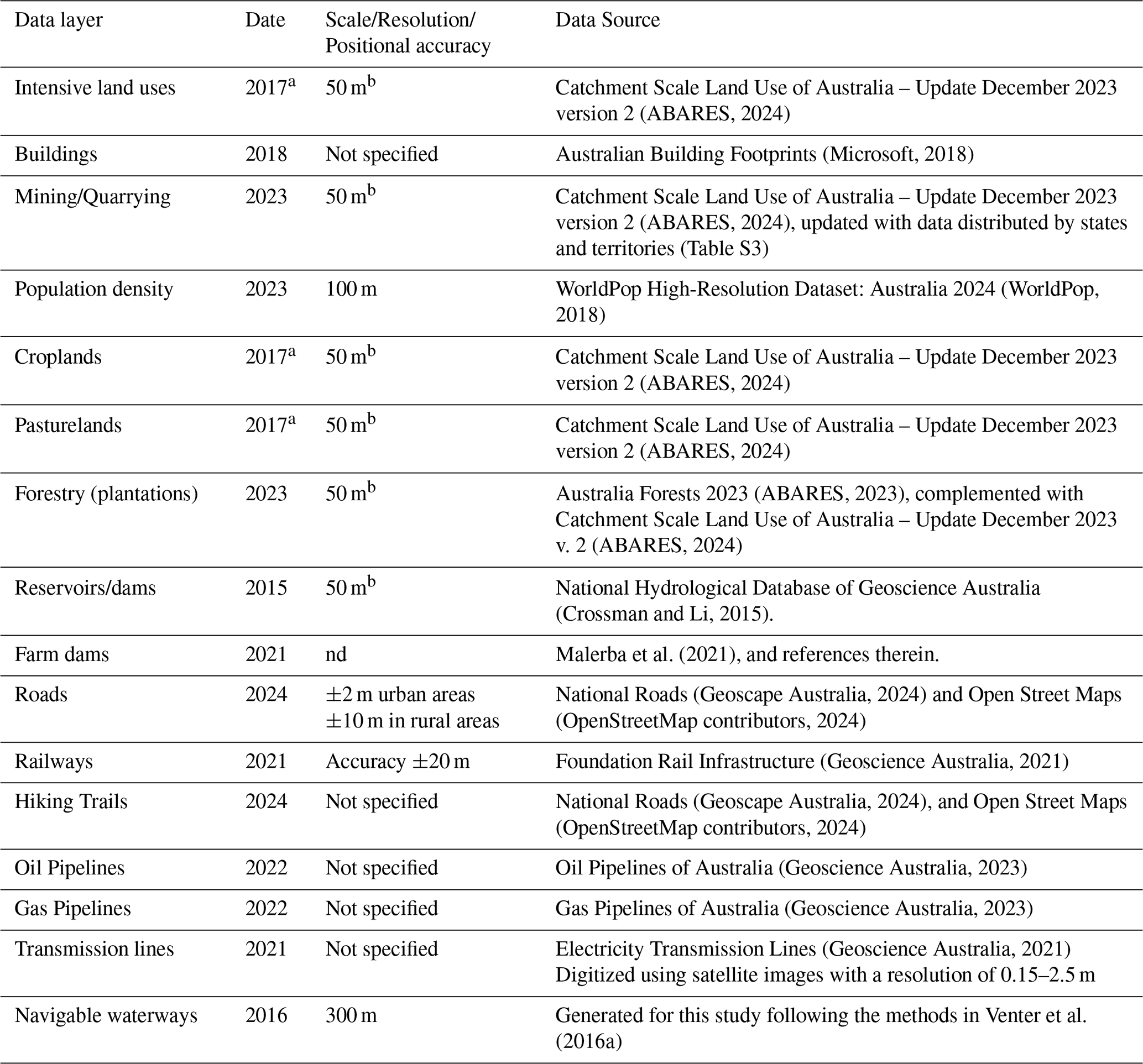
^a Median year of all pixels mapped within the pressure layer, as the date of mapping varies between 2008 and 2023. ^b A seamless raster was created by combining land use vector data showing a single dominant land use for each location based on the management objective of the land manager. The scale of mapping varies between 1 : 50 000 and 1 : 250 000.

Following previous human footprint maps, we defined intensive land uses, mining, cropland, and pasturelands as mutually exclusive pressures, as each represents a complete replacement of natural land cover, unlikely to co-occur with the others within the 100 m pixels used for mapping. Moreover, reservoirs and farm dams are also mutually exclusive, as are paved, unpaved roads, and hiking trails. All other pressure overlaps were allowed to overlap, mainly because they represent additional disturbances that can co-occur spatially in the 100 m pixels used in our analyses (e.g., roads, pipelines, or population density). To avoid spatial overlap among incompatible land uses, we applied a hierarchical rule in which overlaps were resolved by retaining the pressure with the highest intensity score (0–10), for example: built environments ≥ mining > cropland > pastureland. This ensured that only one of these mutually exclusive land-use pressures contributed to each pixel's cumulative score, while allowing other co-occurring pressures to be summed cumulatively.

After creating the weighted pressure layers, we summed them up to generate the terrestrial Human Industrial Footprint map. The analysis was conducted at a 100 m spatial resolution using the Australian Albers Equal Area projection (EPSG:3577). This resolution represented a balance between the 50 m resolution of the primary land use data and the overall accuracy of the dataset. We used a binary rule to rasterise (using gdal_rasterize, with the -at option) polygon and line features to 100 m raster cells, where any pixel intersecting a feature was assigned the corresponding pressure value. All individual layers were processed using GRASS GIS (GRASS Development Team, 2024) or Google Earth Engine (Gorelick et al., 2017). The uncertainty analysis was conducted in Python 3.6 (Van Rossum and Drake, 1995), and graphics were developed using the R Package ggplot (Wickham, 2016).

2.2 Mapped pressures

In this subsection, we outline the rationale for including each of the 16 pressures used in this analysis, the scores assigned to them, and a short description of the data used to represent each pressure. We took advantage of the 2023 update of the Catchment Scale Land Use of Australia (ABARES, 2024), henceforth called CLUMP 2023, to represent several pressures. CLUMP 2023 has a high level of thematic detail (its tertiary classification has 189 classes), uses a standard national classification (Australian Land Use and Management, ALUM Version 8) developed under the Australian Collaborative Land Use and Management Program (ACLUMP), and is updated regularly (e.g., previous updates include 2015, 2017, 2018, and 2020). Although distributed as a 50 m raster, CLUMP 2023 is derived from detailed vector datasets produced by each State and Territory government, through a bottom-up mapping process that combines aerial and satellite images, cadastral and tenure information, zoning data, expert input, and field validation. The vector datasets span various dates (2008–2023) and mapping scales (1 : 5000 to 1 : 250 000) (Fig. S2 in the Supplement), reflecting differences in land-use intensity and regional update cycles. The national raster was generated by the Australian Bureau of Agricultural and Resource Economics and Sciences (ABARES) in ArcGIS, so that each 50 m cell represents a single dominant land use based on the management objective of the land manager. We resampled this dataset to 100 m resolution using a majority filter.

While CLUMP 2023 integrates data of varying scale, age, and jurisdictional origin, it provides a robust, nationally standardised and accepted representation of land use with strong alignment to official State and Commonwealth reporting. Older and coarser data correspond with arid and semi-arid regions where land use changes are less frequent. Therefore, we supplemented these data with more recent, higher-resolution datasets to improve accuracy and currency in these regions. For example, South Australia's arid zones, which rely on older, coarser mapping, are dominated by large expanses of native pasturelands, and changes in pressures can be captured using current and finer data on buildings, farm dams, mines, roads, and other linear infrastructure. A notable modification from previous applications of the HIF methodology is the exclusion of nightlight data as a proxy for infrastructure in rural areas or working landscapes like mine sites (Venter et al., 2016b). We opted not to use nightlights because equivalent or higher-quality national datasets already map these features directly (e.g., CLUM 2023, Geoscience Australia's pipelines and building footprint layers).

Although some of the input datasets differ slightly in their reference years, most represent conditions between 2017 and 2023 and together provide an up-to-date national view of cumulative industrial pressures. These small temporal differences reflect the different update cycles of national and state agencies, but because most pressures (such as infrastructure, land use, and mining) are long-lasting features, they are unlikely to meaningfully affect the overall spatial patterns of pressure across Australia.

2.2.1 Intensive land uses

This category includes pressures from land uses typically linked with infrastructure and human settlements, such as residential, industrial, intensive horticulture and animal production (e.g., glasshouses, piggeries), and the infrastructure supporting services and utilities. Lands affected by these pressures are often heavily modified and constructed, making it unlikely they will revert to a natural state. These areas experience significant disruption of natural processes, leading to habitat loss and the exclusion of wildlife and ecosystem services (Venter et al., 2016a, b). Therefore, we assigned intensive land uses a score of 10. These pressures were mapped using the CLUMP 2023 dataset, which aggregates land use data from 47 tertiary classes (Table S4) into this category. This category broadly aligns with the “Built-up” pressure identified in other human industrial footprint analyses (Sanderson et al. 2002; Venter et al. 2016; Hirsh-Pearson et al., 2022).

2.2.2 Buildings

Buildings remove natural habitat under the footprint of the construction site and are often associated with habitat clearing in areas surrounding the buildings. Here, we assigned a score of 10 to any pixel overlapping a building, which assumes some modification around the building in pixels not fully occupied by its footprint. This pressure was used as a proxy for human settlement and industrial activities outside urban areas that are potentially not captured through coarser mapping by CLUMP 2023. Building data was obtained from Microsoft (2018), which reports a false positive ratio of ∼ 1 % in 1000 randomly sampled buildings. We conducted our own visual inspection of 1000 buildings and observed false positives, especially in arid regions, where big rocks were misidentified as buildings. To reduce these errors, we limited our analysis to buildings located within 200 m of roads or mining areas, as these are typically associated with built structures. We acknowledge that this filtering may produce a slight underestimation of pressures in remote areas where small buildings exist, but roads are unmapped.

2.2.3 Mining and quarrying

Multiple activities associated with mining, from exploration to post-closure, will negatively affect biodiversity and ecosystem services (Boldy et al., 2021; Sonter et al., 2018). Mining reshapes the landscape, alters waterways and wetlands, increases erosion, and causes pollution from noise, dust, and emissions (Haddaway et al., 2019, and references therein). Due to these multiple environmental impacts, we assigned a score of 10 to the direct pressures from mining. To create the mining pressure layer, we updated the mining land use class from the CLUMP 2023 dataset with state-level datasets (see Table S3 for data sources). Note that while most mining data occupies the affected area, some polygons represented the mining tenement, which, while a limitation, captures activities such as human habitation and road construction.

2.2.4 Human population density

Environmental degradation in a particular area is often associated with proximity to human populations due to activities such as recreation, hunting, logging, and the introduction of non-native species. Following Venter et al. (2016b), we converted a human population density layer into a pressure layer with scores between 0 and 10. Locations with more than 1000 people km⁻² were assigned a score of 10, assuming population density reaches saturation at this level. For areas with densities below 1000 people km⁻², we scaled the pressure score logarithmically using the formula: Pressure Score = 3.333 ⋅ log (population density + 1). We used the WorldPop dataset (WorldPop, 2018), which provides population density estimates at a 100 m resolution for its most recent update.

2.2.5 Croplands

Croplands are often completely converted ecosystems and are subject to high levels of pesticide and fertilizer use and destructive slash-and-burn techniques, and as a consequence, have become the main driver of biodiversity decline and the degradation of the natural landscape (Green et al., 2005; Maxwell et al., 2016). Following Venter et al. (2016b), we assigned croplands a pressure score of 7, as some native species can still utilize croplands (Grass et al., 2019), unlike in most built environments. We obtained cropland data from the CLUMP 2023 dataset using 56 tertiary classes associated with these activities (Table S5). We acknowledge that different crops might exert different pressure intensity on the environment, and while our study maintains consistency with what has been done in previous HIF studies, future work could explore modifying cropland pressures based on intensification levels and biochemical conditions.

2.2.6 Pasturelands

Grazing impacts ecosystems through the creation of fence networks, soil compaction, trampling, and intensive browsing of native vegetation, the spread of invasive species, and altered fire regimes (Kauffman and Krueger, 1984). Domestic herbivores also have multi-trophic effects on plant and animal biodiversity, contributing to biodiversity loss (Filazzola et al., 2020). In this study, we diverged from previous human-industrial footprint analyses (Venter et al., 2016b), which assigned a uniform score of 4 to pasturelands. Instead, we made a distinction between modified and native pasturelands under production, a classification provided in the CLUMP 2023 dataset.

Modified pasturelands, characterized by 50 % or more dominant exotic species and irrigation practices (ABARES, 2016), were assigned a score of 6 due to significant vegetation modification and frequent livestock grazing (see Table S6 for CLUMP 2023 tertiary classes). Native pasturelands, which have undergone minimal or no deliberate modification, were assigned a score of 2. This lower score was assigned to native pasturelands to be conservative, as there might be a great similarity between pasturelands in arid zones not often grazed and areas not classified as grazing lands. Data on livestock stocking density and grazing intensity are largely unavailable, making further differentiation within this land use impossible. However, these areas are still associated with varying levels of fencing, soil compaction, and browsing by farmed animals, unpaved roads, and altered fire regimes, which have an associated impact on their native ecological communities (Tulloch et al., 2023).

Spatially explicit national data (e.g., from the Australian Bureau of Statistics) are lacking, and livestock distribution in large arid regions are highly variable through time. Global datasets such as the Gridded Livestock of the World (GLW4; FAO, 2022) and Annual Global Gridded Livestock Mapping, 1961–2021 (Du et al., 2025) were not included due to their coarse resolution (5–10 km), their somewhat outdated baseline, and inability to capture local or seasonal livestock movements. We therefore relied on CLUMP 2023 to represent grazing pressure, and we acknowledge this limitation in the Discussion.

2.2.7 Forestry plantations

Australia's plantation forests covered 1.96×10⁶ ha in 2016, mainly comprising exotic pines (softwood) and Eucalyptus (hardwood) (ABARES, 2018). Plantation forests remove habitat for species, including tree cavities, and can alter paths of travel and fire regimes (Bradstock et al., 2002; Brockerhoff et al., 2008). Given that these plantations are (typically) monocultures, we assigned a pressure score of 7, akin to croplands. The forestry pressure layer was created by merging the CLUMP 2023 dataset, using only the plantation forest classification, with plantation forests from the Australia Forests 2023 dataset (ABARES, 2023). These layers were merged as we argue they complement each other. The CLUMP 2023 dataset does not include some plantations observed in the Australia Forests 2023, while the Australia Forest 2023 dataset does not include plantations that have been recently clear-cut and are presently bare land, but that will most likely be replanted. We did not account for pressures from forestry undertaken in native forests, as spatially explicit records of activities in these areas are not consistently mapped across the continent.

2.2.8 Reservoirs and dams

Dams and reservoirs inundate the land, altering their hydrology and often converting terrestrial ecosystems into aquatic ones, causing habitat loss for many terrestrial and freshwater species, as well as altering local ecosystems (Barnett and Adams, 2021; Poff and Hart, 2002). Dams can also disrupt sediment transportation and fish migration, change water quality, and increase the risk of invasive species (Bunn and Arthington, 2002; Johnson et al., 2008; Liermann et al., 2012; Syvitski et al., 2005). Given this, we assigned reservoirs (including the dam wall area where present) a pressure score of 8. While we focused on the direct pressure from the inundated footprint, we also established a 500 m buffer, where the score is assigned using an exponential decaying function. Furthermore, while dams also exert pressures downstream, we do not consider this in the current analysis, as data for Australia is unavailable. Data for these pressures were obtained from the National Hydrological Database of Geoscience Australia (Crossman and Li, 2015), which was created in 2015 and updated in 2025.

2.2.9 Farm dams

Farm dams (sometimes called “agricultural ponds”) in the Australian agricultural landscape are ubiquitous; Malerba et al. (2021) found over 1.765 million dams across the country, covering an area of 4678 km² and storing more than 20 times the amount of water in Sydney Harbour. These human-made features catch and store water for livestock, irrigation, crop spraying, firefighting, and other domestic purposes. But, while often small in scale, farm dams can significantly affect biodiversity and biogeochemical cycles (Liddicoat et al., 2022; Woolmer et al., 2008). They directly modify the environment, accumulate pollution from run-off, and can produce greenhouse gases.

We assigned a score of 5 to farm dams, which is extended to 500 m from the dam to account for changes to environmental processes. The buffer assumes a conservative distance of concentrated grazing, trampling, and degradation associated with access to water points by livestock which can extend up to 3 km (Cowley et al., 2015; Materne et al., 2025; Washington-Allen et al., 2004); 65 % of farm dams overlapped pasturelands. It also assumes potential spillage during intense rainfall which creates tides of water and, in some cases, flooding when multiple dams are present (Kazarovsky, 1996; Pisaniello and Tingey-Holyoak, 2017). We do not consider downstream pressures due to data availability, and because many farm dams are constructed off-stream (Sect. 2.2.8). We obtained farm dam data from Malerba et al. (2021), who compiled it from different State sources.

2.2.10 Roads

Roads exert numerous direct and indirect pressures on terrestrial and aquatic ecosystems, including habitat loss, fragmentation, mortality from construction, roadkill, animal behavior change, alteration of the physical and chemical environment, spread of invasive species, and increased use of areas by humans (Rytwinski and Fahrig, 2015; Trombulak and Frissell, 2000). This linear infrastructure has direct and indirect pressures on the environment, which are accounted for in the pressure scoring. We adapted the scoring systems for roads from Venter et al. (2016a) to assign these direct and indirect pressure scores and differentiate between sealed and unsealed roads, as we recognize that many roads in regional areas are rarely used. A score of 8 was assigned to a 0.3 km buffer from sealed roads and a decreasing pressure from 7.9 to 0.25 outward up to 5 km from the road. Unsealed roads were assigned a score of 3, including a 0.3 km buffer from the road and a decreasing pressure from 2.9 to 0.25 outward up to 5 km from the road. The 5 km maximum distance follows Arias-Patino et al. (2024), based on observed road impacts on mammals; for instance, in Australia McCall et al. (2010) reported that sugar glider survival was ∼ 70 % lower within 5 km of major roads. This distance also serves as a proxy for accessibility and is consistent with recent human-footprint mapping efforts (Hirsh-Pearson et al., 2022), while remaining more conservative than early global maps (Venter et al., 2016b; Williams et al., 2020). However, we acknowledge that this is a major simplification, since off-road accessibility varies with topography, land tenure, land cover, and hydrology. Future pressure mapping in Australia could explore the use of friction-surface and travel-time models (Nelson et al., 2019; Weiss et al., 2020).

To create the roads layer, we merged the National Roads dataset (Geoscape Australia, 2024) and the Open Street Map (OpenStreetMap contributors, 2024) data. Integrating two road datasets introduces the possibility of “double-counting” when the same road is represented in both datasets, due to the features not spatially aligning exactly within the two datasets; however, because we are rastering linear features at a 100 m pixel size, small errors in alignment are most likely removed. Larger spatial alignment errors of the same feature, where found, may be representative of the real-world nature of unsealed roads and tracks in rural and outback areas in Australia, where road users may seasonally take different paths due to high water levels or other factors. Full SQL attribute and data tag queries used for each road type (sealed, unsealed, track, patch) and for each input dataset, can be found in Tables S7–S8 in the Supplement.

2.2.11 Railways

Like roads, railways are linear infrastructures that directly remove habitat, resulting also in fragmentation that can produce edge effects (Fuentes-Montemayor et al., 2009). However, railways are less conducive to providing access to natural environments than roads, given that passengers would usually only disembark at rail stations. The direct pressure of railways was assigned a pressure score of 8, with a 50 m buffer on either side of the railway. We used data from the Foundation Railway of Australia (Geoscience Australia, 2021), which includes open, closed, and other tracks. We removed features with a dismantled, proposed, or disused status from this dataset.

2.2.12 Hiking trails

We also included the disturbance from trails, as these are often pathways for human access-related pressures (hunting, invasive weeds, etc.) into remote and protected areas. We assigned a low direct pressure score of 0.9 to trails to acknowledge their presence while remaining conservative in estimating human pressures in remote areas. This conservative weighting reflects both the variable quality and completeness of trail data across jurisdictions and expert input from wilderness mapping practitioners, who note that limited or infrequently used trails may not substantially compromise wilderness character. To create the trails layer, we merged the National Roads dataset (Geoscape Australia, 2024) and the Open Street Map (OpenStreetMap contributors, 2024) data, using the query described in Tables S7–S8.

2.2.13 Transmission lines, and oil and gas pipelines

Pipelines and transmission corridors represent important linear infrastructure that exerts multiple pressures on natural systems. Their construction and maintenance lead to habitat loss and fragmentation of natural habitats and can facilitate the spread of invasive species (Benítez-López et al., 2010). Moreover, pipeline leaks and spills can pollute the soil and water and contribute to greenhouse gas emissions (Brandt et al., 2014). Transmission lines can affect the mortality of flying animals (Bevanger, 1998) and increase the risk of wildfires (Keeley and Syphard, 2018). We believe these linear features represent pressures in a similar way to unsealed roads (and often have unsealed service roads alongside them). Therefore, we set a direct pressure score of 3 with a buffer of 300 m around this type of infrastructure and an indirect score decaying from 3 to 0.25 outwards to 2.5 km from the infrastructure (Arias-Patino et al., 2024).

2.2.14 Navigable waterways

Navigable waterways – in the form of navigable rivers, lakes, and marine coastlines – facilitate human accessibility to the natural environment in a way analogous to roads. We created the navigable pressure layer by applying the methods described in Venter et al. (2016a, b), on a 100 m resolution. Areas directly alongside navigable waterways have a pressure of 4, which decreased exponentially outwards 15 km (Venter et al., 2016a, b).

2.3 Technical validation and uncertainty (sensitivity) analysis of the Human Industrial Footprint

2.3.1 Validation and accuracy assessment

We followed the methods outlined in Arias-Patino et al. (2024) and Venter et al. (2016a, b) to evaluate the agreement between the HIF map and the pressures observed in situ. To this end, a single assessor visually identified industrial pressures observed through very high-resolution satellite images (<1 m, typically 0.3–0.5 m in urban and coastal areas) within 1397 randomly stratified sample plots. The satellite images were obtained from web map services such as Google Maps, Bing Maps, and the ArcGIS Basemap, corresponding to imagery from 2020–2023.

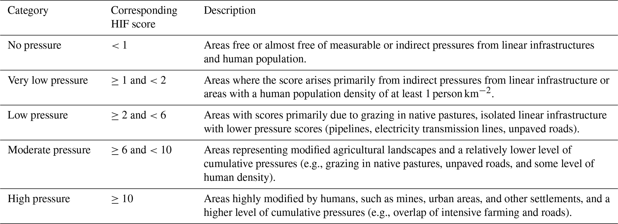
We defined five strata corresponding to pressure classes (Table 2), allocating a number of samples to each, following Olofsson et al. (2013, 2014), distributing them according to the area and expected error for each stratum. This strategy aims to prevent oversampling large strata like low-pressure areas and minimize the standard error for small regions like high-pressure areas, which could result in an overestimation of the accuracy. Because the stratified random sampling was based on HIF value ranges, the validation sample is not entirely independent of the resulting map. However, this approach ensured that the full gradient of cumulative pressures was represented, particularly in low- and high-pressure areas that occupy small proportions of Australia's land area. Each sample location was selected randomly within strata, and validation relied on independent, very high-resolution satellite imagery, providing an objective assessment of accuracy.

Table 2 The HIF was classified into five descriptive categories representing diverse levels of pressure.

The sample distribution was as follows: no pressure = 477, very low pressure = 30, low pressure = 565, moderate pressure = 205, high pressure = 120. Each sample plot consisted of a 100 m window (matching the analysis' spatial resolution) and five surrounding buffers at 300, 500, 1000, 2750, and 5000 m to aid in recording both direct and indirect pressures (Arias-Patino et al., 2024). Scores were assigned as per Table S9. Indirect pressures were recorded based on the nearest observed feature and its area of influence, with scores assigned using the mean value of the two closest buffers. The sum of all observed pressure scores represented each plot's assumed actual state of in-situ pressures, while corresponding HIF values were extracted from the map for comparison.

Both HIF and validation scores were normalized to a 0–1 scale using the min–max normalization formula. We used the maximum value observed in our map rather than the theoretical maximum, as there is no location where all pressure factors overlap simultaneously, following Venter et al. (2016a, b). To quantify the level of agreement between the HIF and validation scores, we utilized the root mean square error (RMSE) (Chai and Draxler, 2014). The RMSE expresses the average error in the units of the variable of interest, tending to penalize large errors; a lower RMSE indicates higher agreement between the HIF and the validation scores. We also calculated the percentage of validation samples with agreement between the HIF and validation scores, considering the HIF to match the validation score if they were within 20 % of each other on the 0–1 scale (Venter et al., 2016b). This ±20 % tolerance provides a complementary measure of continuous-scale agreement, offering an intuitive indication of how close predicted and observed values are before categorization. It does not replace the categorical accuracy metrics outlined below, but adds context to the RMSE and R² results by highlighting overall precision and bias trends.

Finally, we also conducted an accuracy assessment of the classified five-level HIF map to provide a complementary perspective focused on the reliability of the pressure classes used for spatial interpretation and conservation planning. Using the same validation samples, we estimated the user's, producer's, and overall accuracy metrics using the proportion of area, as implemented in the “mapaccuracy” R package (Costa, 2024). Agreement was determined by whether each sample plot fell within the same pressure class in both the HIF and the visual interpretation. The accuracy assessment also allowed us to produce error-adjusted estimates of the area for each class (Olofsson et al., 2013), supporting future applications that rely on categorical representations of the HIF. This accuracy was done, as numerous research studies have applied thresholds to cumulative pressure maps to categorize the level of human influence and inform conservation interventions at different scales. For example, it has been used to identify the last of the wild (Sanderson et al., 2002), the most globally intact areas (Watson et al., 2016; Williams et al., 2020), wilderness areas and vegetation condition assessments in Australia (Lesslie et al., 1988; Lesslie and Taylor, 1985; Thackway and Lesslie, 2008), and to assess the extinction risk to species (Di Marco et al., 2018).

2.3.2 Uncertainty analysis

To understand the degree of uncertainty in our results, associated with the scores assigned to the different pressures, we followed Arias-Patino et al. (2024) and randomly adjusted intensity scores in the validation samples, by up to ±50 % using the bootstrap technique. We chose to adjust pressure scores by up to ±50 %, a wider range than the ±30 % used by Arias-Patino et al. (2024), in order to test the robustness of our cumulative pressure scores under a wider range of values. This approach allowed us to evaluate whether the model remains stable even when pressure intensity values are varied well beyond the expected range of expert-derived variability. Each simulation involved selecting a random factor between 0.1 % and 50 %, which was then applied to each pressure layer. Specifically, we multiplied this factor by the original pressure intensity (PI) value for each layer and randomly added or subtracted the result from the validation sample. We adjusted the pressure intensity (PI) by layer (s) as follows.

$$\begin{array}{}\text{(1)}& \begin{array}{rl}& \mathrm{Modified}{\mathrm{PI}}_s={\mathrm{PI}}_s\pm \left({\mathrm{PI}}_s\times n\right);\\ & n=\mathrm{random}\mathrm{number}\mathrm{between}\mathrm{0.01}\text{–}\mathrm{0.5}\end{array}\end{array}$$

Using the modified scores, we calculated the simulated cumulative pressure value for each validation plot containing mapped values and then assessed the error by comparing it to the original mapped values. This simulation was repeated 100 000 times to ensure statistical robustness. Finally, we generated an uncertainty map by interpolating the standard deviation of the error using the inverse distance weighting (IDW) technique.

2.3.3 Comparison with Global Human Footprint datasets

To assess the added value of the fine-scale national Human Industrial Footprint (HIF), we carried out a visual comparison with global Human Footprint datasets available at 1 km for 2013 (Williams et al., 2020) and at 100 m resolution for 2020 (Gassert et al., 2023). These comparisons were used to qualitatively evaluate how well the HIF captures the spatial patterns of cumulative pressures relative to global assessments. Because the datasets differ in resolution, input data, set of mapped pressures, and some assumptions, interpreting a direct quantitative comparison is of limited value.

2.4 The ecological intactness index

When pressure maps such as the HIF are used as proxies of ecological condition or intactness, it is done based on thresholds applied to individual pixels with a certain pressure value (Watson et al., 2016; Williams et al., 2020). However, while the HIF incorporates some indirect pressures that spread out to a buffer from the direct pressure, the value of each pixel does not explicitly account for the spatial configuration and habitat-quality context surrounding that pixel. For example, a narrow strip of native vegetation between agricultural fields could appear to have no pressure because there is no indirect pressure for cropland in the HIF; however, such a strip is impacted by significant edge effects and unmapped human presence, indicating it is somewhat degraded and not intact as the HIF would indicate. Here, we overcome this by calculating an intactness metric (Beyer et al., 2020) for Australia, which is sensitive to changes in habitat area, quality, and fragmentation (and therefore captures the structural component of ecological integrity (Nicholson et al., 2021), which is well known to influence the ability of an area to support a diversity of species (Betts et al., 2017; Fischer and Lindenmayer, 2007; Hanski et al., 2013).

For each 100 m cell, intactness was estimated as a function of the spatial configuration and quality of surrounding habitat, with contributions from neighbouring cells declining with distance. The metric is parameterized to decrease monotonically with increasing fragmentation, reflecting both the number and separation of habitat patches, and to scale with total habitat area and quality. The HIF served as the base layer, normalized to a 0–1 scale and inverted so that higher values represent greater habitat quality (i.e., lower pressure). Intactness values were computed within a circular moving window of 5 km radius using the kernel function described by Beyer et al. (2020), which integrates both patch size and isolation effects. The resulting EII represents the relative degree to which each location retains the spatial configuration and quality characteristic of structurally intact ecosystems.

3 Results

3.1 Human Industrial Footprint map and pressures overview

The Australian Human Industrial Footprint Index (Fig. 2a) map covers an area of 7 692 047 km² and has a spatial resolution of 100 m. The scores range between 0 (areas with no mapped pressures) and 56.5 (densely populated built-up urban regions), with a mean score of 3.05 ± 4.18, and a median of 2.25. The HIF scores are highly skewed to low values, as seen in the classified map (Figs. 3, S3), which shows that more than one-third of the Australian landscape (32 %) is free or almost free (score < 1) of the 16 pressures included in this analysis, and another 2.9 % experiences very low pressures (i.e., scores of <2) (Fig. 3). Another 47.5 % of the Australian landscape has a low industrial pressure footprint (HIF value ≥ 2 and <6). These low-pressure areas are primarily pastoral leases that operate without extensive introduction of non-native pastures. However, this analysis does not account for stocking intensity, and we acknowledge that the pressure in some of these areas might be underestimated. Finally, 14.2 % of the Australian landscape presents more considerable industrial pressures (scores ≥ 6), with 5.6 % of the land being under moderate pressure (scores between 6 and 10) and a further 8.5 % experiencing high industrial pressure (scores ≥ 10).

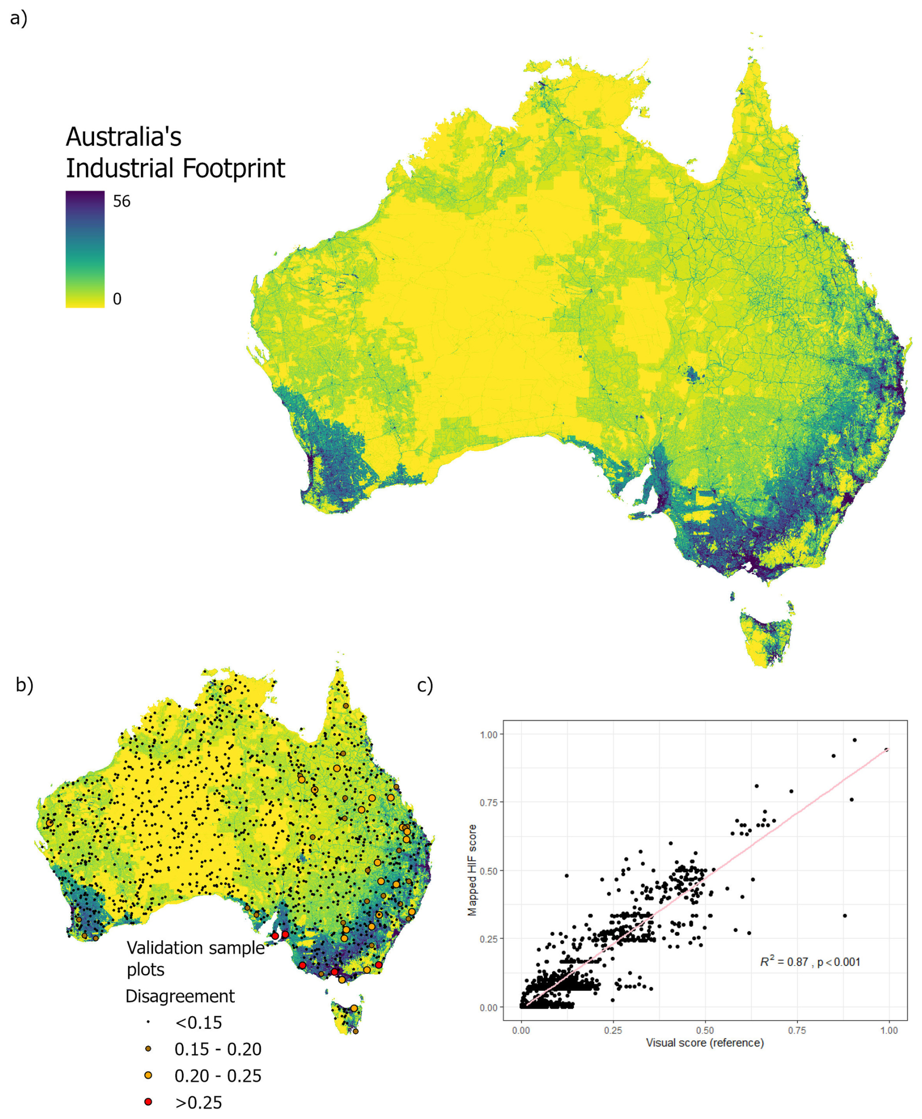
Figure 2 (a) Australia’s Human Industrial Footprint map on land. (b) Location of the validation sample plots used for the technical validation. Larger points indicate plots where the HIF and the visual score differed by more than 20 % on a normalized (0–1) scale. (c) Relationship between the reference score (visual interpretation) and the score obtained from the HIF for Australia.

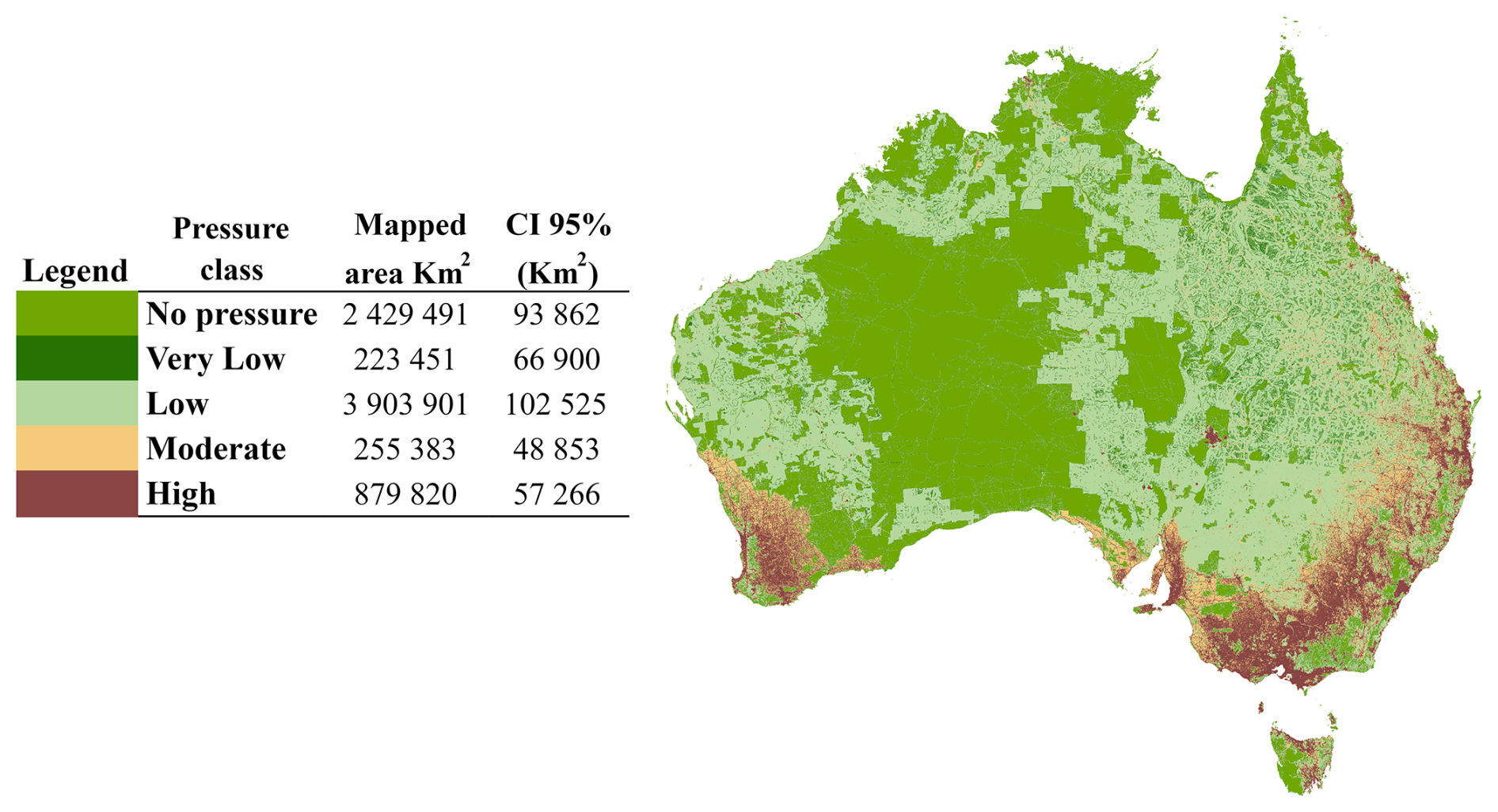
Figure 3 Australian Human Industrial Footprint map categorized into five industrial pressure classes, from no pressure to high pressure (see Table 2). The table shows the error-adjusted area, and 95 % confidence intervals estimated for each class.

The most prevalent pressures in Australia, in terms of areal coverage, are roads and grazing in native pastures, which exert some level of pressure across approximately 66 % and 46 % of the nation, respectively (Table 3).

Table 3 The percentage of the mapped area that each pressure covers across the Australian landscape.

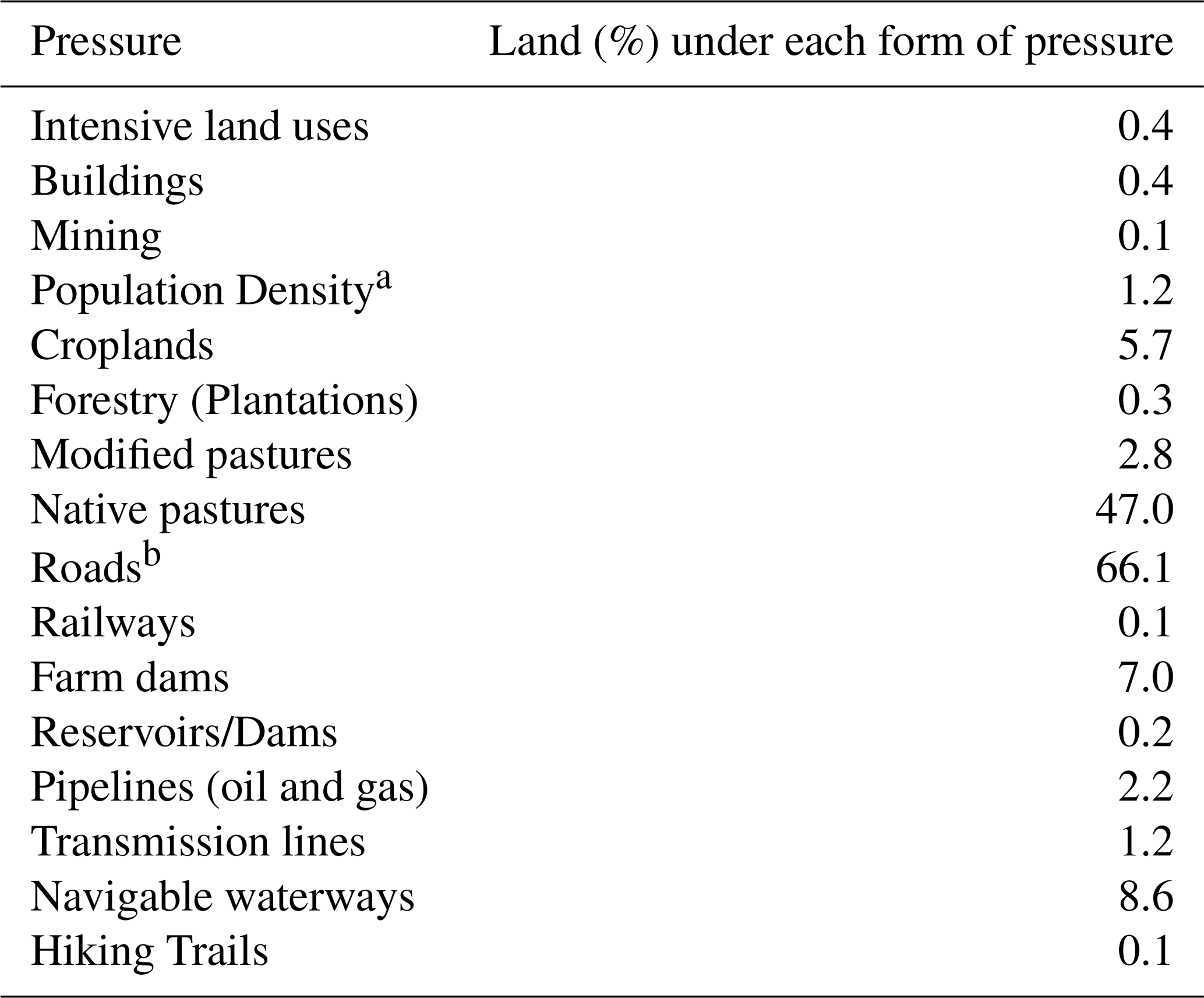
^a A population density score of 0.1 (out of 10), corresponding to a population density of ∼ 0.1 persons km⁻² was used as a threshold to define the presence of this pressure in a pixel. If the threshold is not applied, scores as low as 0.001 will be quantified, and the total area (%) of land affected by this pressure will increase to 95 %. ^b Paved and unpaved roads were aggregated to calculate this statistic.

3.2 Technical validation

The technical validation results indicate a strong agreement between the Human Industrial Footprint scores and those obtained through visual interpretation. A strong relationship (R²=0.87) exists between the human industrial footprint and the validation scores (Fig. 2b). The RMSE for the 1397 validation plots was 0.059 on the normalized 0–1 scale, indicating an average deviation of approximately 6 %. In addition to these continuous measures, 98 % of validation plots showed agreement within ±20 % between the HIF and the observed scores, providing an intuitive indication of how closely the mapped values match on-the-ground conditions. Only 27 plots fell outside this range (Fig. 2a), five higher and 22 lower than the observed score, suggesting the HIF tends to underestimate pressure. Even when we consider a stricter threshold of 15 % for agreement, we still obtained a 96.2 % match between the HIF and the visual scores.

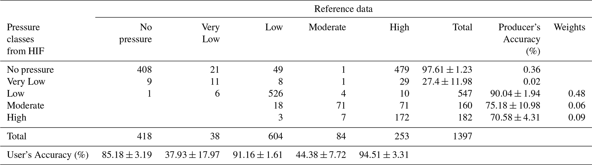
The overall accuracy of the classified map is 85.0 %, where most errors arise from the HIF underestimating the in-situ pressure observed during the visual inspection of high-resolution satellite images (Table 4). These suggest that the HIF can be considered a conservative estimate of human pressures on the environment. Moreover, the confusion matrix shows that the very low-pressure class has both low producer's and user's accuracy, indicating the difficulty of detecting low-impact activities that can occur in highly intact landscapes.

Table 4 Error matrix showing the performance of a thematic map of five pressure classes obtained from the classification of the HIF against the pressure class obtained from the reference data (visual scores), using sample counts (for an error matrix estimated by proportions of area see Table S10). Accuracy measures are presented with a 95 % confidence interval, and the overall accuracy was 85 %.

Overall, the combination of continuous and categorical validation metrics demonstrates that the HIF map achieves practical reliability for mapping the cumulative industrial pressures at a national scale that were considered here.

3.3 Uncertainty in pressure values

Changes in the pressure scores had only a limited impact on the cumulative pressure values. Adjusting the scores, either increasing or decreasing them by up to 50 %, resulted in a moderate difference (error) between simulated and mapped values (mean = 0.002 ± 1.129). The maximum and minimum errors observed were 2.745 and −2.57, respectively, representing slightly above one-quarter of the full pressure scale.

Across the 100 000 simulations, nearly 90 % of validation plots with mapped features (Fig. 4) exhibited errors within a narrow range, between −0.15 and 0.16 (corresponding to the 5th and 95th percentiles). As expected, larger adjustment factors led to increased variability; however, even at the maximum adjustment level of 50 %, 73 % of plots still displayed relatively small errors (ranging from −2.5 to 2.5). The uncertainty map (Fig. 5) shows that areas where multiple pressures converge, particularly densely populated regions near major cities, are more vulnerable to uncertainties in pressure values. Higher uncertainties in areas with high HIF values likely reflect the accumulation of positional and classification errors from overlapping layers and the fine-grained heterogeneity typical of developed landscapes.

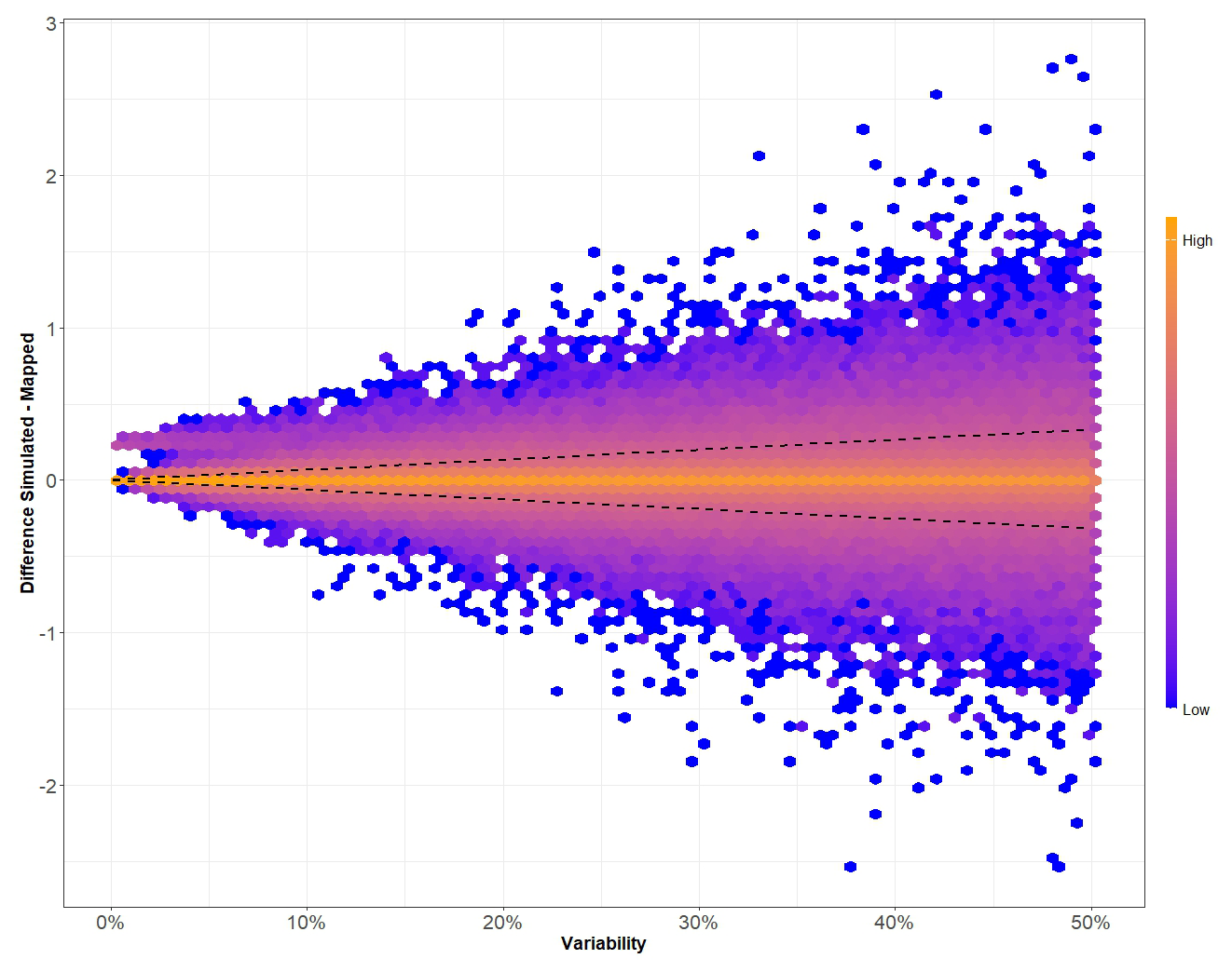
Figure 4 Density plot depicting the difference between simulated value and mapped value (y-axis) relative to the percentage of variability of pressure scores (x-axis). The color scale represents the number of plots that include this transition, with orange indicating a high number of plots and blue indicating a few plots (legend is log-scaled). Black dashed lines represent the 5th and 95th percentiles of the distribution of the difference. Plots with no mapped features were excluded from the analysis.

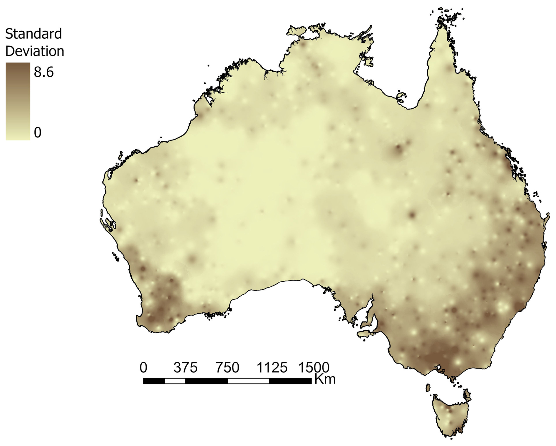
Figure 5 Spatial distribution of the uncertainty of pressure scores across Australia when these are increased or decreased by 50 %. Darker tones represent areas with high standard deviation of the mean cumulative pressure value.

3.4 Comparison with global footprint datasets

A visual comparison between the national HIF and the global Human Footprint maps at 1 km and 100 m resolutions reveals broadly similar patterns of cumulative pressures across the continent. However, clear mismatches are evident even at a coarse scale. For instance, large parts of inland Australia appear pressure-free in the global maps, yet these areas coincide with native pasturelands captured in the Australian analysis (Fig. 6a). At finer scales, differences become more apparent, arising both from the coarser resolution of the 1 km dataset and from the inclusion of additional nationally curated pressures in the HIF. Examples include Kangaroo Island (Fig. 6b) and the city of Townsville and its surroundings (Fig. 6c), where the national HIF captures unpaved roads, forestry, and pasturelands that are absent in the global products. The Australian HIF also shows finer detail in cumulative pressures within urban centres and peri-urban areas, where features such as farm dams, reservoirs, and unpaved roads are more accurately represented.

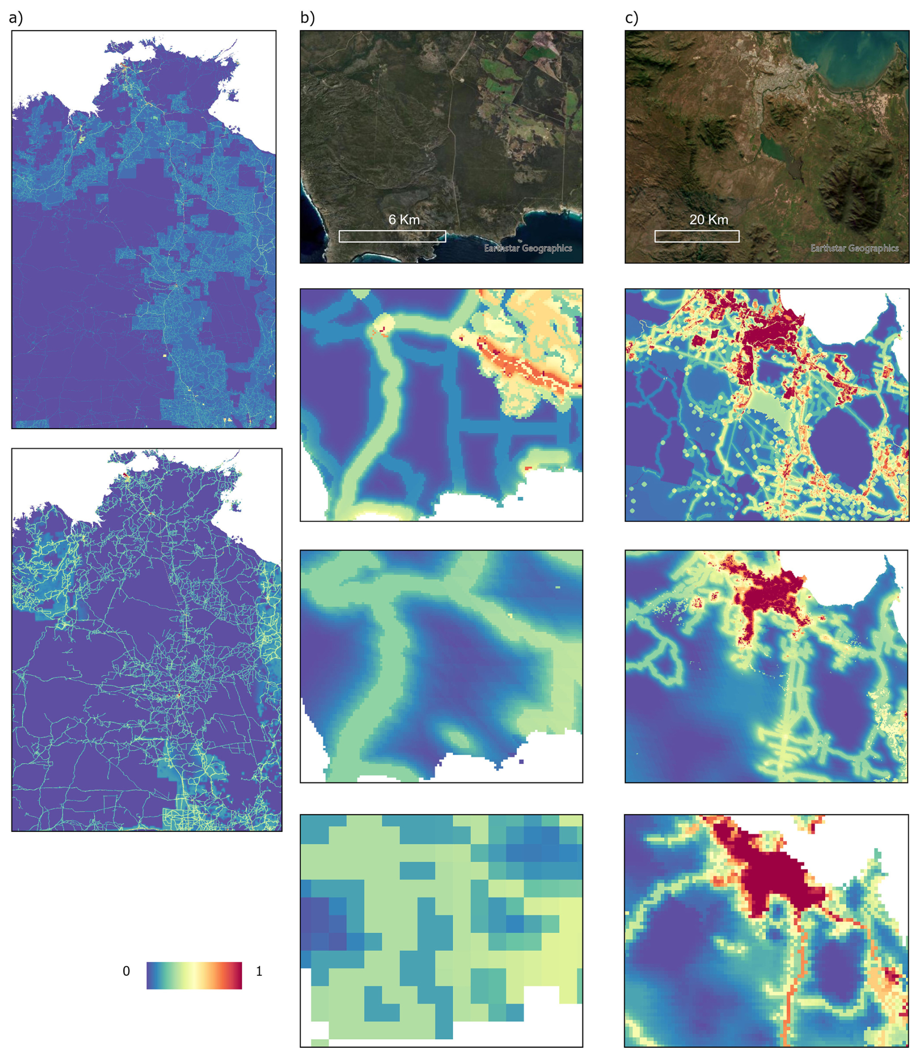
Figure 6 Comparison between the Australian Human Industrial Footprint (HIF) and global Human Footprint datasets. (a) Continental-scale comparison showing extensive areas where the Australian HIF (top) maps pressures from grazing in native pasturelands that are not visible in the global products (bottom). (b) Regional example for Kangaroo Island, South Australia, illustrating improved representation of pressures such as unpaved roads, forestry, and pasturelands in the national HIF relative to global datasets. (c) Urban and peri-urban examples for Townsville, Queensland, showing that the national HIF captures finer-scale gradients of disturbance and additional features such as reservoirs, farm dams, and unpaved roads. Values range from 0 (low pressure) to 1 (high pressure). From top to bottom in (b) and (c) are satellite imagery of the area of interest, followed by the Australian HIF, the global 100 m, and the global 1 km datasets, respectively.The imagery displayed is World Imagery from ArcGIS Map Service, and the source is Esri, Maxar, Earthstar Geographics, and the GIS User Community.

3.5 Ecological Intactness Index

The Ecological Intactness Index map for Australia (Fig. 7) covers the same area as the HIF and was calculated using the same spatial resolution of 100 m. The mean intactness value obtained through this map for Australia is 0.52 ± 0.32 (on a scale of 0 to 1, with 1 representing high intactness). Approximately 60.5 % of the country has an EII value of <0.5, with 9.4 % of the landscape experiencing the most severe levels of degradation (EII < 0.1). The inset maps show how the EII value varies in areas with no mapped pressures, depending on the spatial configuration and habitat-quality context surrounding each pixel, to provide a surrogate of structural intactness.

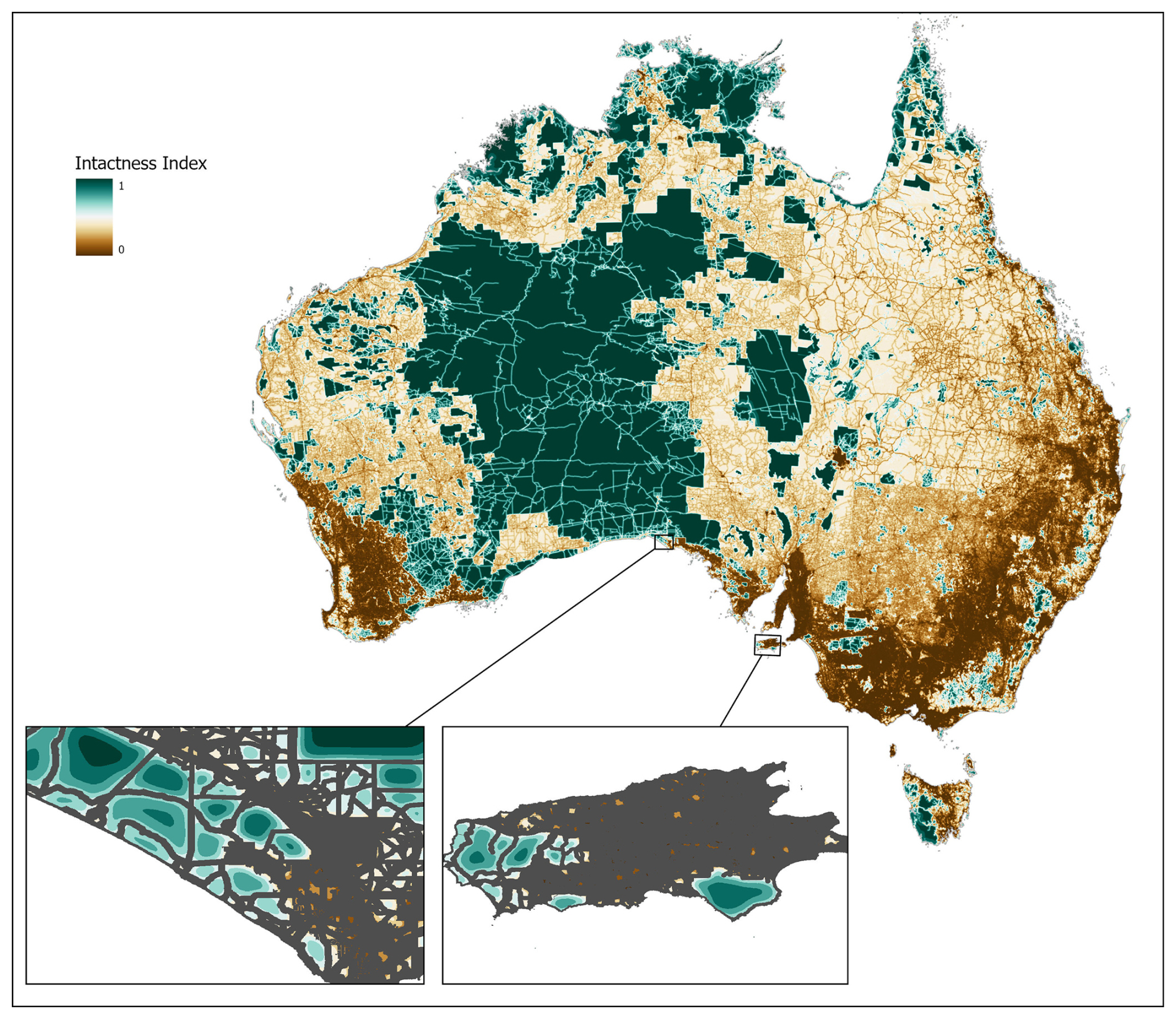
Figure 7 Ecological intactness index map for Australia calculated based on Beyer et al. (2020) using the Australian Industrial Footprint as an input habitat condition layer. The two inset maps show that, despite some areas not having observable industrial pressures (areas with mapped pressures are in grey), their intactness values depend on the habitat quality (HIF value) of surrounding pixels.

4 Discussion

We present two complementary national datasets: the Human Industrial Footprint (HIF), the first national cumulative pressure map since the National Wilderness Inventory of the 1980s and 1990s (Lesslie and Taylor, 1985), and the complementary Ecological Intactness Index (EII), a map to represent ecological structural intactness across the nation. Both extend the established Human Footprint framework (Sanderson et al., 2002; Venter et al., 2016a, b) using nationally curated and thematically detailed inputs, harmonised under a consistent scoring and validation approach at a 100 m spatial resolution.

The HIF represents a cumulative model of industrial pressures rather than direct ecological conditions. High HIF values indicate areas with greater concentration or intensity of human activities, often associated with degraded states of natural systems; low values indicate areas with fewer detectable or less intense pressures, associated with intact states. As in previous studies, HIF values should be interpreted ordinally, not linearly (Watson et al., 2016; Williams et al., 2020). For example, a pixel with a value of 20 does not imply that it experiences double the pressure compared to a pixel with a value of 10; rather, it can be assumed to be experiencing a higher level of cumulative disturbance. The classified HIF map provides an intuitive framework for communication and comparison across regions, facilitating policy and planning, and has been used for many diverse conservation applications, including determining species' risk of extinction and the degree of human influence on protected areas (Allan et al., 2022; Jones et al., 2018; Di Marco et al., 2018; Torres-Romero et al., 2025).

The EII complements the HIF by translating mapped pressures into an estimate of ecological intactness, capturing fragmentation and degradation, without reference to specific pressures. It has been used to guide protected area expansion, restoration planning, and application of the mitigation hierarchy (Mappin et al., 2019; Venegas-Li et al., 2024), and, as an indicator to the GBF, will help nations measure progress toward global conservation goals related to integrity.

We do note that cumulative impact maps remain imperfect representations of the complex human-environment interactions (Halpern and Fujita, 2013). They are constrained by the quality and completeness of the underlying datasets and by the assumptions made to integrate them. All these are fully documented here to ensure transparency and reproducibility, and we provide all data and code to openly encourage refinement and improvements as new information becomes available.

5 Limitations and Uncertainty

While comprehensive, the product we present here is subject to several limitations. Some are inherent in cumulative pressure mapping (Watson et al., 2023b); others reflect the data used and assumptions in this analysis. Our analysis does not account for all pressures, either because we lacked suitable data to represent them, or because we focused on those that are observable and related to access by humans. Excluded pressures include individual oil and gas wells, invasive species, disease, pollution, climate change, changes in groundwater regimes, and fire-regime shifts.

Consequently, some areas mapped as intact could be severely affected by unmapped disturbances. Similarly, the ecological response to equivalent pressures likely varies among ecosystems, meaning HIF values indicate potential rather than realized impacts. This being said, the HIF has been shown to be an excellent proxy for assessing species extinction and ecological degradation (see discussion in Watson et al., 2023b). We also note that rasterising vector data at 100 m resolution introduces a degree of generalisation, particularly for narrow linear features such as roads and pipelines, which may occupy only a fraction of a pixel. This can slightly overestimate their direct footprint, although we make the assumption that, in most cases, the ecological influence of such infrastructure extends beyond this area.

In the methods section, we outlined the specific limitations of each data set and the assumptions we made, but we discuss some in more detail here. Roads and grazing in native pasturelands are the two most prevalent pressures in the Australian landscape, but remain imperfectly mapped. Although we merged the Geoscape National Roads and OpenStreetMaps data, a close inspection using high-resolution satellite images shows that many unpaved and private roads are missing, and the completeness of the data varies between states and territories. For example, rural roads in New South Wales appear to be better mapped than in the adjoining areas in Queensland and South Australia, likely underestimating pressures in those regions. Grazing intensity in native pastures is poorly documented in Australia; we therefore applied a conservative pressure score of 2, which might underestimate the degree of pressure in some areas.

One key concern with additive methods for mapping cumulative pressure maps is the use of expert judgment to assign pressure intensity scores to each spatial layer (Halpern and Fujita, 2013; Korpinen and Andersen, 2016). To minimize subjectivity, we adopted scoring approaches from established, peer-reviewed global and national studies (Arias-Patino et al., 2024; Hirsh-Pearson et al., 2022; Venter et al., 2016b; Woolmer et al., 2008), and apply them consistently via open scripts. To further address concerns about subjectivity and its influence on the final cumulative pressure scores, we conducted a comprehensive uncertainty analysis. Following the methodology of Arias-Patino et al. (2024), we tested robustness by varying all scores by up to ±50 % across 100 000 simulations; nearly 90 % of validation plots showed errors within a narrow range, indicating low sensitivity to reasonable variations in pressure score inputs. Future refinements could employ structured expert elicitation or data-driven calibration to strengthen scoring schemes.

Although cumulative pressure maps necessarily simplify complex human-environment interactions, the framework applied here is grounded in more than two decades of peer-reviewed development and remains widely used across ecological science and environmental decision-making (Watson et al., 2023b). As outlined above, future national assessments will be strengthened through integration of fire-regime metrics, invasive-species layers, and livestock-intensity data as they become available. These improvements will become increasingly feasible as higher-resolution national datasets continue to emerge. Importantly, pressure and ecological intactness layers derived from cumulative pressure maps continue to support contemporary applications in biodiversity risk assessment, conservation priority-setting, and protected-area evaluation (Canassa et al., 2025; Forti et al., 2025; Presotto et al., 2025; Ramírez-Delgado et al., 2025; Torres-Romero et al., 2025), emphasizing both the practical reliability and ongoing relevance of the approach.

6 Data availability

The datasets generated from this work are available at Zenodo https://doi.org/10.5281/zenodo.17606284 (Venegas-Li et al., 2025). It is provided in a standard raster format (tif).

7 Code availability

The code to create the individual pressure layers and the human footprint are available through the same repository (Venegas-Li et al., 2025, https://doi.org/10.5281/zenodo.17606284).

8 Conclusions

The Human Industrial Footprint (HIF) and Ecological Intactness Index (EII) developed in this study provide a contemporary assessment of cumulative pressures accross Australia's landscapes and a proxy for ecological degradation at 100 m resolution. These datasets offer valuable insights for understanding human impacts on biodiversity and ecosystem intactness and degree of degradation, addressing a long-standing gap in national-scale pressure mapping. By incorporating 16 nationally relevant pressure layers, the HIF provides a more accurate and context-specific representation of industrial influences than global-scale analyses, improving our ability to guide conservation and land-use planning. Both layers should be of interest to all those involved in biodiversity management when considering Australia's Strategy for Nature 2024–2030 (Commonwealth of Australia, 2024) and Nature Positive Plan (DCCEEW, 2022), as well as its global commitments to the Kunming-Montreal Global Biodiversity Framework with respect to Targets 1–4 especially (CBD, 2022). By identifying areas of high intactness and those under significant industrial pressure, these datasets can inform protected area expansion, ecosystem restoration priorities, and biodiversity offset strategies. Beyond conservation policy, the HIF and EII have applications in environmental impact assessments, regional land-use planning, and climate adaptation and mitigation strategies. Their integration into national and subnational decision-making processes can help halt further biodiversity loss, improve connectivity between protected areas, and support sustainable development objectives.