A multi-year global methane data set obtained by merging observations from TROPOMI and IASI

Data products of atmospheric methane (CH₄) with improved vertical sensitivity in the lower troposphere are crucial for gaining a more comprehensive understanding of the impact of anthropogenic emissions. This study presents a CH₄ data product derived from the synergetic combination of level 2 (L2) data from TROPOMI (Tropospheric Monitoring Instrument) and IASI (Infrared Atmospheric Sounding Interferometer), specifically CH₄ total column and CH₄ profiles, respectively. IASI enables high-quality observation of CH₄ mixing ratios in the upper troposphere and lower stratosphere, and TROPOMI observations excel in providing sensitivity to the total column-averaged mixing ratio of CH₄. By combining the IASI and TROPOMI L2 products synergetically, we can detect tropospheric CH₄ (mixing ratios averaged over a layer representing the lowermost 50 % of the atmosphere) that is not significantly affected by the strong CH₄ variations around the tropopause. This is not achievable by using IASI or TROPOMI data alone.

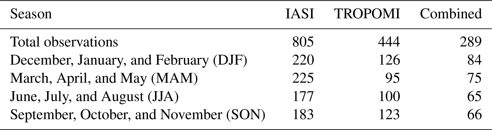
For the synergetic L2 data combination, we use the method as presented in detail in Schneider et al. (2022b), and apply it to combine about 444 million individual and high-quality TROPOMI observations with about 805 million individual and high-quality IASI observations made globally over 42 months (from January 2018 to June 2021). The combination method is fast; it uses a tool designed for efficient geo-matching between large data sets and a computationally cheap Kalman filter for merging the data sets. We show that the combined data set has a good global coverage. Moreover, we document that the sensitivity (response of the combined data product to real atmospheric CH₄ variations) is very satisfactory throughout the globe, and the uncertainties are generally below 12–15 ppbv. Furthermore, we demonstrate the increased scientific value of the combined data product when compared to the two individual data products.

The data set of the combined product consists of about 289 million individual data points, and it is provided as NetCDF files. One file has a typical size of 85 MB and contains all data for observations made in one day (the universal time of the TROPOMI observations are taken as the reference time). The data set is referenced to https://doi.org/10.35097/wq583rnzpmd83m5g (Shahzadi et al., 2026) and also made freely available at https://www.imk-asf.kit.edu/english/CH4-synergy-IASI-TROPOMI_RemoTeC.php (last access: 8 March 2026).

1 Introduction

The abundance of remote sensing data offers a valuable opportunity to explore and exploit the diversity of data sets. One can increase the scientific impact of such data by integrating them and by leveraging their different characteristics (like different sensitivities or error patterns). The integration of diverse data sets can lead to strong synergies, i.e. a new data set having advanced sensitivities and/or reduced errors.

For an optimal synergetic combination of two data sets, the precise knowledge of the characteristics of the two individual data sets is essential. Concerning level 2 (L2) remote sensing data, we can only successfully combine the data sets, if each data point is made available together with its error (or error covariances), sensitivity/representativeness (i.e. the averaging kernels) and information on a priori choices.

The vertical sensitivity of satellite remote sensing data of trace gases depends heavily on the spectral region of the observation. For instance, the Infrared Atmospheric Sounding Interferometer (IASI) aboard the Metop satellites measures nadir spectra in the thermal infrared region and has a high spatial resolution with global coverage twice daily. IASI has a good sensitivity of trace gas variations in the free troposphere and the lower stratosphere (e.g. Clerbaux et al., 2009). However, it lacks sensitivity in the lower troposphere due to low thermal contrast near surface.

Data generated from observations of the Tropospheric Monitoring Instrument (TROPOMI) aboard the Sentinel-5 Precursor satellite are promising for complementing this deficit in the IASI data. TROPOMI offers a similar good spatial resolution and coverage as IASI, but it observes Earth surface reflected solar spectra in the near infrared region (e.g. Veefkind et al., 2012). TROPOMI offers good sensitivity throughout the whole atmosphere and provides total column-averaged trace gas products at a good quality.

Schneider et al. (2022b) shows that the well-characterised IASI and TROPOMI methane (CH₄) L2 data products can be successfully combined, and the combined product is superior to the individual data products. The combination retains the good data quality of CH₄ in the free troposphere and lower stratosphere (offered by the IASI product), and of the CH₄ total column (offered by the TROPOMI data). In addition, it yields good-quality tropospheric CH₄ data which is not observable in the two individual data products. Schneider et al. (2022b) applied the method to locations and periods with collocated reference observations of TCCON (Total Carbon Column Observing Network, Wunch et al., 2011a), AirCore (Karion et al., 2010), and GAW (Global Atmospheric Watch), and performed an extensive validation and inter-comparison study.

In this study, we present a data set generated with the Schneider et al. (2022b) method using IASI and TROPOMI observations from January 2018 to June 2021, which results in a very large synergetic multi-year global data set. In Sect. 2, we present the two individual satellite data sets used for generating a synergetic product, and discuss their main characteristics and coverages. Section 3 briefly describes the method used for the synergetic data set combination and presents the achieved data coverage. Section 4 documents the vertical representativeness of the TROPOMI, IASI and the combined data products, thereby revealing the synergetic gain achieved by the data combination. In Sect. 5, we present the leading errors and Sect. 6 compares the temporal and spatial patterns of the combined data products, demonstrating their additional scientific potential on top of the individual TROPOMI and IASI data products. Section 9 gives a summary and outlook.

2 Input data products

2.1 MUSICA IASI

We use a data product obtained from measurements of IASI, a remote sensing instrument on board of the Metop series of satellites. IASI detects the infrared radiations that are emitted by the Earth and transported throughout the atmosphere. We use the IASI CH₄ L2 data product generated by the retrieval processor MUSICA (García et al., 2018; Schneider et al., 2022a) developed at the Karlsruhe Institute of Technology (KIT). MUSICA stands for “MUlti-platform remote Sensing of Isotopologues for investigating the Cycle of Atmospheric water” which is a project intialised and developed under the framework of the European Research Council (project phase 2011–2016). The MUSICA IASI full retrieval data product versions 3.2 and 3.3, used here, includes trace gas profiles of H₂O, the HDO/H₂O ratio, N₂O, CH₄, and HNO₃. The data are provided together with detailed information on a priori usage, constraint, averaging kernels and error covariances for each individual observation. The footprint pixel at nadir has a diameter of 12 km and IASI offers twice daily global coverage over both the land and ocean. Figure 1 shows the coverage for June, July and August (JJA) in (a) and for December, January and February (DJF) in (c). Some data gaps are observed over dry stony/sandy regions, like the Sahara desert. There are significant number of retrieval results filtered out due to poor quality of the respective spectral fits. The reason for this poorer fit quality is the weak and poorly-decribed infrared surface emissivity of stony/sandy ground (e.g. Zhou et al., 2011). MUSICA IASI version 3.2 and 3.3 data are described in detail in Schneider et al. (2022a) and made freely available for October 2014 to July 2021 (Schneider et al., 2021). Here, we work with the period from January 2018–June 2021, which is the time when TROPOMI data are available along with MUSICA IASI's.

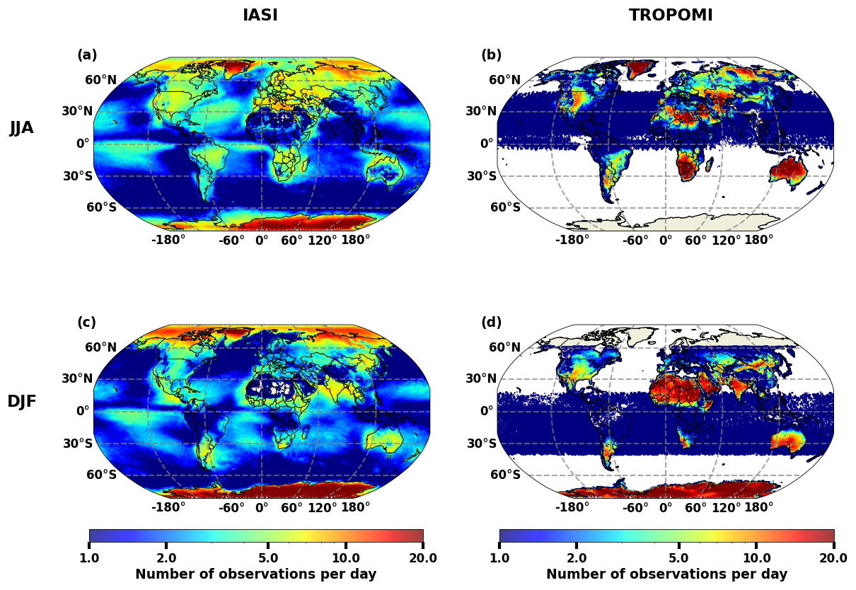
Figure 1 Average daily number of observations per 50 km × 50 km grid boxes for IASI (a, c) and TROPOMI (b, d). (a, b) June, July, and August; (c, d) December, January, and February.

We only use the data if the fit quality of the MUSICA IASI retrieval is very good (musica_fit_quality_value is 3), representing high-quality fits for which the spectral residuals are close to the instrumental noise (see Sect. 6 of Schneider et al., 2022a). Furthermore, we require that the EUMETSAT L2 cloudiness assessment summary flag is 1 (IASI field of view is clear) or 2 (IASI field of view is processed as cloud-free but small cloud contamination is possible). In the latter case, we require additionly an EUMETSAT L2 fractional cloud cover value of 0.0 or NaN. The total amount of individual IASI CH₄ L2 data used in this study from the January 2018–June 2021 period is aproximately 805 million observations. Table 1 gives an overview on the data volumes.

2.2 RemoTeC TROPOMI

The second data set is the TROPOMI total column-averaged methane mixing ratios (XCH₄) generated by the retrieval algorithm RemoTeC (Butz et al., 2011; Lorente et al., 2021) at the Space Research Organisation Netherlands (SRON). The TROPOMI data processing was carried out with the Dutch National e-infrastructure with the support of the SURF cooperative. TROPOMI is aboard the Sentinel-5 Precursor (S5P) satellite and provides data since 2018. For this study, we use the beta version of the operational S5P product (Lorente et al., 2023a), which uses an updated fit of the surface reflectance spectral dependency to a third-order polynomial fit. The data are made freely available at https://doi.org/10.5281/zenodo.7766558 (Lorente et al., 2023b).

The mean data coverage for January 2018–June 2021, particularly for the seasons JJA and DJF is shown in Fig. 1b and d. TROPOMI offers a near-global coverage over land at the resolution of 7 km × 7 km since its launch in October 2017 (upgraded to 5.5 km × 7 km in August 2019). Over ocean, observations are only possible in glint mode, which leads to much less frequent observations. Its coverage also differs seasonally. For example, no data are available at high latitudes over winter hemispheres, because high solar zenith angles are filtered out and TROPOMI cannot observe during polar night. Data coverage over land is best in the subtropics and worst in the tropics, which can be explained by a strict cloud filtering. The TROPOMI XCH₄ L2 data is available with the column averaging kernels, errors and an a priori CH₄ profile data. These a priori data are calculated by the global chemistry transport model TM5 (Krol et al., 2005). We use TM5 a priori data as the common TROPOMI and IASI CH₄ a priori data, i.e. we adjust the IASI product to the TROPOMI a priori data using the additive post-processing a priori correction as suggested in Rodgers (2000) and Rodgers and Connor (2003). In order to exclude data of a compromised quality, we only use the TROPOMI data that have a quality flag value (qa_value) of 1.0. In this study we use about 444 million TROPOMI observations made between January 2018 and June 2021 (for more details on the data volumes see Table 1).

Table 1 Table summarizing data volumes (number of observations) in million. The values are given for the whole 42 months (All) and separately for the different seasons. DJF: December, January, February; MAM: March, April, May; JJA: June, July, August; SON: September, October, November

3 Synergetic data product

In this section, we briefly describe the method used for combining the IASI and TROPOMI L2 data, and present the data amount and coverages of the combined data product. We use the validated method as described in Schneider et al. (2022b). So far, the method has only been applied for creating small data sets (representing individual months or limited areas). Here we apply the method to create a much more substantial data set.

3.1 Geomatching

Figure 2 depicts the whole workflow for combing the IASI and TROPOMI L2 data. In a first step, we identify the IASI observation that best matches in time and space with a given TROPOMI observation, i.e. we have to optimally geomatch the data sets. This is a significant challenge for large data sets and we developed a dedicated geomatching algorithm based on the work of Ameri et al. (2014). The geomatching requires metadata information such as spatial, temporal and sensor-specific attributes of the individual sensors, which are stored in a MongoDB database. We chose MongoDB due to its flexible handling of semi-structured JSON-like data, native support for spatial queries, and horizontal scalability. These features enable a fast selection of daily observations and a simplified geospatial filtering during the initial matching phase, depending on the distribution strategy employed and the availability of computational resources. The metadata are loaded as in-memory data frames using Python’s Pandas library (McKinney, 2010) for further processing. Afterwards, vectorised-distance calculations, using haversine distance, is implemented to identify IASI observations near each TROPOMI point within the defined temporal window. In a first geomatching step, we use all IASI observations, within 50 km (horiziontal distance), 50 hPa (surface pressure difference), and 6 h (observation time difference) of a single TROPOMI observation. These requirements are generally fulfilled for many different IASI observations (see example of all matches in Fig. 2). In a second geomatching step, we select the optimal match as the minimum of the Euclidean distance calculated from normalized horizontal distances, time differences, and surface pressure differences (a single IASI observation is remained as the optimal match, see example of Fig. 2). The normalization for the horizontal distance is 50 km, for the temporal distance it is 2 h, and for the surface pressure difference it is 5 hPa.

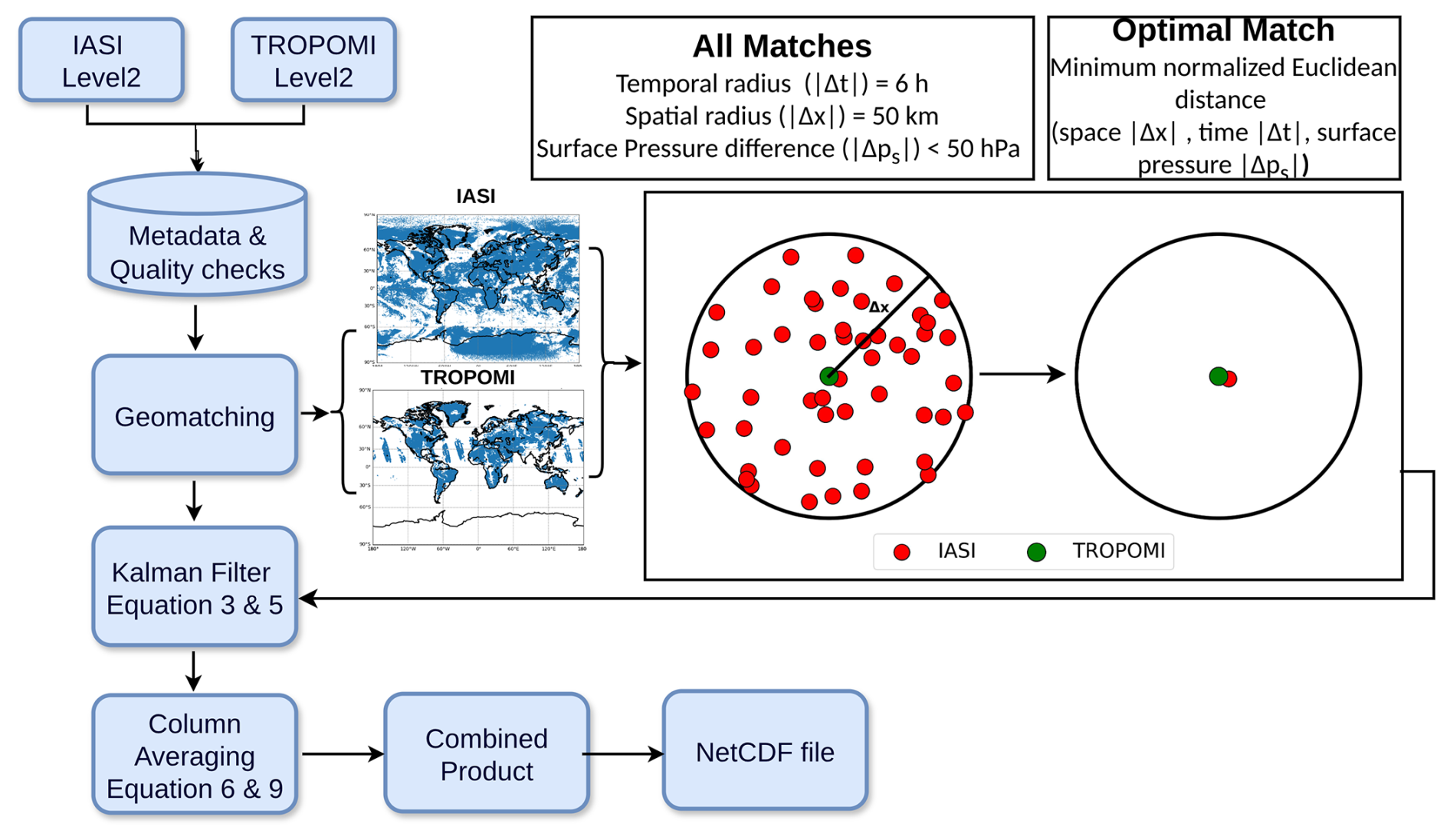
Figure 2 Schematic workflow for combining IASI and TROPOMI level 2 data. Metadata from both sensors that pass the quality checks are stored in MongoDB. A geomatching procedure then filters all IASI observations for each TROPOMI pixel for spatial ($\mid \mathrm{\Delta }x\mid$), temporal ($\mid \mathrm{\Delta }t\mid$) and surface pressure ($\mid \mathrm{\Delta }{p}_{\mathrm{s}}\mid$) difference radius of 50 km, 6 h and 50 hPa, respectively. The optimal match is then selected by minimizing the normalized Euclidean distance (using norms of 50 km, 2 h, 5 hPa, for $\mid \mathrm{\Delta }x\mid$, $\mid \mathrm{\Delta }t\mid$, $\mid \mathrm{\Delta }{p}_{\mathrm{s}}\mid$, respectively). The matched data are subsequently processed using a Kalman filter according to the Eqs. (3) and (5). Then the column averages are calculated according to Eqs. (6) and (9). Finally, the combined products are stored in a NetCDF file.

Figure 3a, c and b, d show the mean spatial and temporal mismatches, respectively, obtained for the optimal matches between TROPOMI and IASI for JJA and DJF. The spatial mismatches are mostly below 30 km, except for regions where IASI data are sparse (e.g. over the Sahara). The temporal mismatches show a clear latitudinal gradient. The temporal mismatches are smallest in middle and high northern latitudes (less than 2 h) and largest in middle southern latitudes (generally more than 4 h). This can be explained by the different orbits of the two satellites that carry the IASI and the TROPOMI instruments.

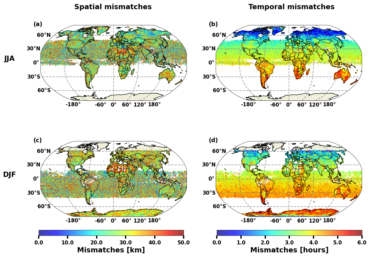
Figure 3 Spatial (a, c) and temporal (b, d) mismatches for the optimal matches averaged per 50 km × 50 km grid boxes. (a, b) June, July and August; (c, d) December, January and February.

3.2 Combination by a Kalman filter

The Schneider et al. (2022b) method uses a Kalman filter to optimally combine the IASI and TROPOMI data. Assuming moderately non-linear IASI and TROPOMI retrieval processes, it has been shown that the method is analogous to performing a retrieval that simultaneously uses the level 1 spectra of TROPOMI and IASI. However, it remains computationally inexpensive and automatically benefits from the most latest improvements made by the individual IASI and TROPOMI retrieval experts.

The Kalman filter approach is analogous to a data assimilation approach, where a background state x^b is improved by adding information provided by a measurement y. The result is the analysed state x^a:

$$\begin{array}{}\text{(1)}& {\mathit{x}}^{\text{a}}={\mathit{x}}^{\text{b}}+\mathbf{G}[\mathit{y}-\mathbf{H}{\mathit{x}}^{\text{b}}],\end{array}$$

where H is the measurement operator that projects the background state onto the measurement domain, and G is a Kalman gain matrix, that describes how inconsistencies between the background state (x^b) and the measurement (y) impact on the analysis state (x^a):

$$\begin{array}{}\text{(2)}& \mathbf{G}={\mathbf{S}}^{\mathrm{b}}{\mathbf{H}}^{\mathrm{T}}[{\mathbf{HS}}^{\mathrm{b}}{\mathbf{H}}^{\mathrm{T}}+{\mathbf{S}}_{\mathit{ϵ}}{]}^{-\mathrm{1}}.\end{array}$$

Here S^b captures the background covariances and S_ϵ are the measurement error covariances.

We apply the Kalman filter as described in Eqs. (1) and (2) to the IASI and TROPOMI CH₄ L2 data. As mentioned in Sect. 2, we use an IASI profile retrieval result obtained by applying the same CH₄ a priori information as in the TROPOMI retrieval (i.e. the TM5 model calculations). The difference between the retrieved IASI profile and this a priori profile is used as the background state (i.e. for x^b we use $({\widehat{\mathit{x}}}_{\mathrm{I}}-{\mathit{x}}_{\mathrm{a}}$) where ${\widehat{\mathit{x}}}_{\mathrm{I}}$ is the retrieved IASI CH₄ profile and x_a the a priori profile). The difference between the retrieved TROPOMI XCH₄ and the a priori XCH₄ is used as the measurement (i.e. for y we use $({\widehat{x}}_{\mathrm{T}}^{*}-x_{\mathrm{a}}^{*})$, where ${\widehat{x}}_{\mathrm{T}}^{*}$ is the retrieved TROPOMI XCH₄ value and ${\widehat{x}}_{\mathrm{a}}^{*}$ is the apriori XCH₄ value). The obtained analysis state is then the difference between the combined profile and the apriori CH₄ profile (i.e. x^a is replaced by $\widehat{\mathit{x}}-{\mathit{x}}_{\mathrm{a}}$). The TROPOMI total column-averaged mixing ratio averaging kernels are used as the measurement operator (i.e. for H we use ${\mathit{a}}_{\mathrm{T}}^{*}{}^{\mathrm{T}}$). With these substitutions Eq. (1) is written as:

$$\begin{array}{}\text{(3)}& \widehat{\mathit{x}}-{\mathit{x}}_{\mathrm{a}}=({\widehat{\mathit{x}}}_{\mathrm{I}}-{\mathit{x}}_{\mathrm{a}})+\mathit{g}\left[\right({\widehat{x}}_{\mathrm{T}}^{*}-x_{\mathrm{a}}^{*})-{\mathit{a}}_{\mathrm{T}}^{*}{}^{\mathrm{T}}({\widehat{\mathit{x}}}_{\mathrm{I}}-{\mathit{x}}_{\mathrm{a}}\left)\right].\end{array}$$

The subindices “I” and “T” stand for IASI and TROPOMI, respectively. The variables with no capital letter subindex stand for the combined product. The subindex “a” indicates the TM5 a priori data and the superindex “^*” marks variables that represent total column-averaged mixing ratio data. Retrieved data are identified by the hat symbol “$\widehat{}$”. The total column-averaged mixing ratio averaging kernel of the TROPOMI product (${\mathit{a}}_{\mathrm{T}}^{*}{}^{\mathrm{T}}$), can be calculated from the respective total column amount averaging kernel (${\mathit{a}}_{\mathrm{T}}^{\mathrm{T}}$, which is distributed within the TROPOMI L2 data set) as follows (see also Appendix D in Schneider et al., 2022b):

$$\begin{array}{}\text{(4)}& {\mathit{a}}_{\mathrm{T}}^{*}{}^{\mathrm{T}}=({\mathit{w}}^{\mathrm{T}}\mathbf{Z}\mathit{w}{)}^{-\mathrm{1}}{\mathit{a}}_{\mathrm{T}}^{\mathrm{T}}\mathbf{Z},\end{array}$$

with w^T being a row vector that integrates the whole column, i.e. it has dimension 1×n (n is the number of atmospheric layers) and all elements have the value 1.0. For converting mixing ratio profiles into amount profiles and vice versa, we need the pressure weighting operator Z. It is a diagonal matrix (dimension n×n) whose elements report the amount of dry air molecules represented by the individual atmospheric layers.

The Kalman gain operator g used in Eq. (3) is:

$$\begin{array}{}\text{(5)}& \mathit{g}={\mathbf{S}}_{\mathrm{I}}{\mathit{a}}_{\mathrm{T}}^{*}{\left({\mathit{a}}_{\mathrm{T}}^{*}{}^{\mathrm{T}}{\mathbf{S}}_{\mathrm{I}}{\mathit{a}}_{\mathrm{T}}^{*}+S_{\mathrm{T},n}^{*}\right)}^{-\mathrm{1}},\end{array}$$

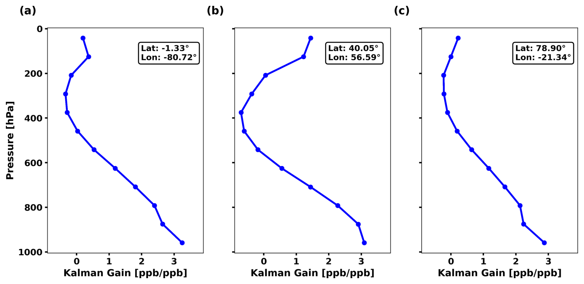
which is obtained by substituting, in Eq. (2), the background covariances (S^b) by the IASI a posteriori covariances (S_I, which can be calculated from the variables provided within the MUSICA IASI L2 netcdf files according to Eq. (A8) of Schneider et al., 2022a). Furthermore, we substitute the measurement error covariance (S_ϵ) by the TROPOMI error variance ($S_{\mathrm{T},n}^{*}$). Equations (3) and (5) are analogous to Eqs. (1) and (2) of Schneider et al. (2022b). For brevity, we omit the transformation from a linear to a logarithmic scale and all variables used in the equations of this manuscript are given in linear scale and all variables as distributed in the netcdf data set files are given in linear scale. Here the Kalman gain vector g is a vector, because the TROPOMI data has only one dimension (it is a total column data product). This Kalman gain describes how inconsistencies between the IASI L2 profile retrieval and the TROPOMI L2 total column data impact on the combined profile data product. Appendix A shows typical Kalman gain vectors for low, middle, and high latitudes. Please note that the calculations according to Eqs. (3) and (5) involve no matrix inversions as the inversion in Eq. (5) applies to a scalar.

The TROPOMI data are provided as total column-averaged mixing ratios (XCH₄). From the IASI and the combined CH₄ profiles, we calculate three different partial column products: the total column-averaged mixing ratio (XCH₄), the tropospheric column-averaged mixing ratio (troXCH₄, representing the layer between the surface and the atmosphere at 50 % surface pressure), and the upper tropospheric and stratospheric column-averaged mixing ratio (utsXCH₄, representing the layer between 50 % surface pressure and the top of atmosphere). The column-averaged mixing ratio CH₄ products refer to the amount of CH₄ integrated over a specific atmospheric layer relative to the amount of dry air in that layer, i.e. it is a dry air mole fraction of CH₄ and it is given in ppbv.

These calculations are made according to

$$\begin{array}{}\text{(6)}& {\widehat{x}}^{*}={\mathit{w}}^{*}{}^{\mathrm{T}}\widehat{\mathit{x}},\end{array}$$

where ${\widehat{x}}^{*}$ is the retrieved column-averaged mixing ratio, $\widehat{\mathit{x}}$ is the retrieved mixing ratio profile (dimension n×1), and w^*T is the pressure weighted resampling operator (dimension 1×n) that resamples the mixing ratio profiles represented in n vertical layers onto an averaged mixing ratio value. The operator w^*T is representative for a certain atmospheric partial column layer and obtained by

$$\begin{array}{}\text{(7)}& {\mathit{w}}^{*}{}^{\mathrm{T}}=({\mathit{w}}^{\mathrm{T}}\mathbf{Z}\mathit{w}{)}^{-\mathrm{1}}{\mathit{w}}^{\mathrm{T}}\mathbf{Z},\end{array}$$

where the vector w integrates the targeted partial column layer. It has the (n×1) dimension, with elements being 1.0 for the layers belonging to the targeted partial column layer and 0.0 for the layers outside of the targeted column layer.

3.3 Data amount and coverage

From the geomatching, we identify about 289 million TROPOMI observations, for which we have a collocated IASI observation (for more details on the data volume see Table 1). The respective data coverage for JJA and DJF is shown in Fig. 4. Occasionally, over land there are more than 5–10 observations per day in a 50 km × 50 km box, except for high latitudes in the winter hemisphere and for the tropics. This coverage is similar to the maps showing the TROPOMI data (Fig. 1b and d), i.e. the coverage of the synergetic data product is strongly determined by the data availability of TROPOMI. Generally, if the TROPOMI data set provides a high-quality data, there is also a closeby high-quality IASI observation available.

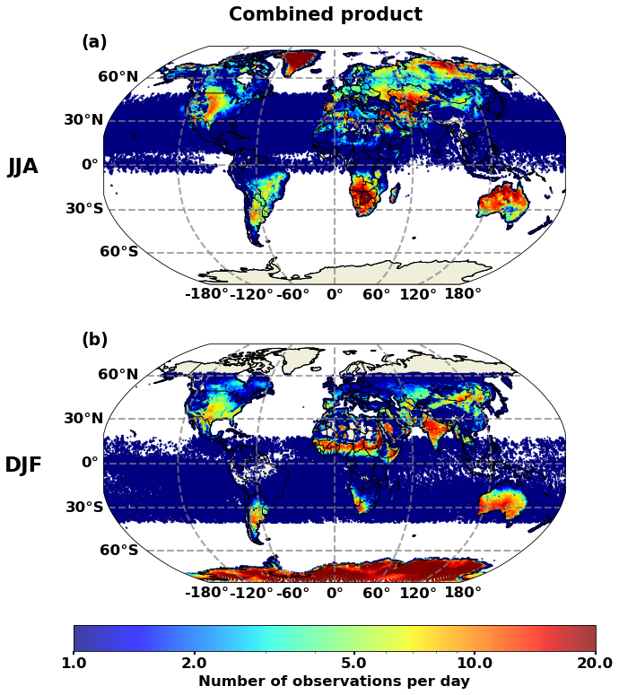
Figure 4 Average daily number of observations per 50 km × 50 km grid boxes for the combined product. (a) June, July, and August; (b) December, January, and February.

4 Vertical representativeness and sensitivity

Atmospheric trace gas remote sensing data products do not represent all the vertical structures (limited vertical representativeness) and they do not always respond to the full amplitude of the real atmospheric trace gas variations (limited sensitivity). These inherent characteristics of trace gas remote sensing products is captured by the remote sensing averaging kernels. Thus, the averaging kernels are indispensable for a correct remote sensing data usage. In this section, we discuss the averaging kernels of the TROPOMI and the IASI data products, and compare it to the respective kernels of the combined data product. Moreover, we document the horizontal pattern of the vertical representativeness and sensitivity.

4.1 Averaging kernels

The TROPOMI data are distributed as a total column-averaged data product (XCH₄) together with a total column amount averaging kernel, which is a row vector a^T of 1×n dimension. This row vector describes how the retrieved total column amount responds to changes of trace gas amounts at a certain layer (by how many CH₄ molecules does the retrieved total total column amount change when adding one CH₄ molecule at a certain layer).

The IASI data are distributed as a vertical mixing ratio profile data product together with its vertical mixing ratio averaging kernels, i.e. for each retrieval layer there is a dedicated averaging kernel that accounts for how a change in mixing ratio in the real atmosphere affects the retrieved mixing ratio profile. This averaging kernel is a matrix A of dimension n×n.

The data combination calculations, as described in Sect. 3.2, also generate a vertical mixing ratio profile. The mixing ratio profile averaging kernel of the combined product can be calculated by (see also Eq. (3) of Schneider et al., 2022b):

$$\begin{array}{}\text{(8)}& \mathbf{A}={\mathbf{A}}_{\mathrm{I}}+\mathit{g}{\mathit{a}}_{\mathrm{T}}^{*}{}^{\mathrm{T}}(\mathbf{I}-{\mathbf{A}}_{\mathrm{I}}).\end{array}$$

Here, A and A_I represent the mixing ratio profile averaging kernel for the combined data and the IASI product, respectively. Appendix B illustrates typical mixing ratio profile averaging kernels for IASI and for the combined data product, for low, middle, and high latitudes. We distribute total and partial column amount averaging kernels with our data set. The TROPOMI L2 data set directly provides the total column amount averaging kernels. For the IASI and the combined data products, we calculate the total and partial column amount averaging kernels (a^T) from the mixing ratio profile averaging kernels (A) according to

$$\begin{array}{}\text{(9)}& {\mathit{a}}^{\mathrm{T}}={\mathit{w}}^{\mathrm{T}}{\mathbf{ZAZ}}^{-\mathrm{1}}.\end{array}$$

4.2 Vertical representativeness

The vertical representativeness of the total and partial column-averaged data products can be documented by the total and partial column amount averaging kernels. Figure 5 shows typical total and partial column amount averaging kernels (a^T) for the individual IASI and TROPOMI products and for the combined product. We define the lowermost 50 % of the atmosphere as the troposphere and the uppermost 50 % of the atmosphere as the upper troposphere/stratosphere.

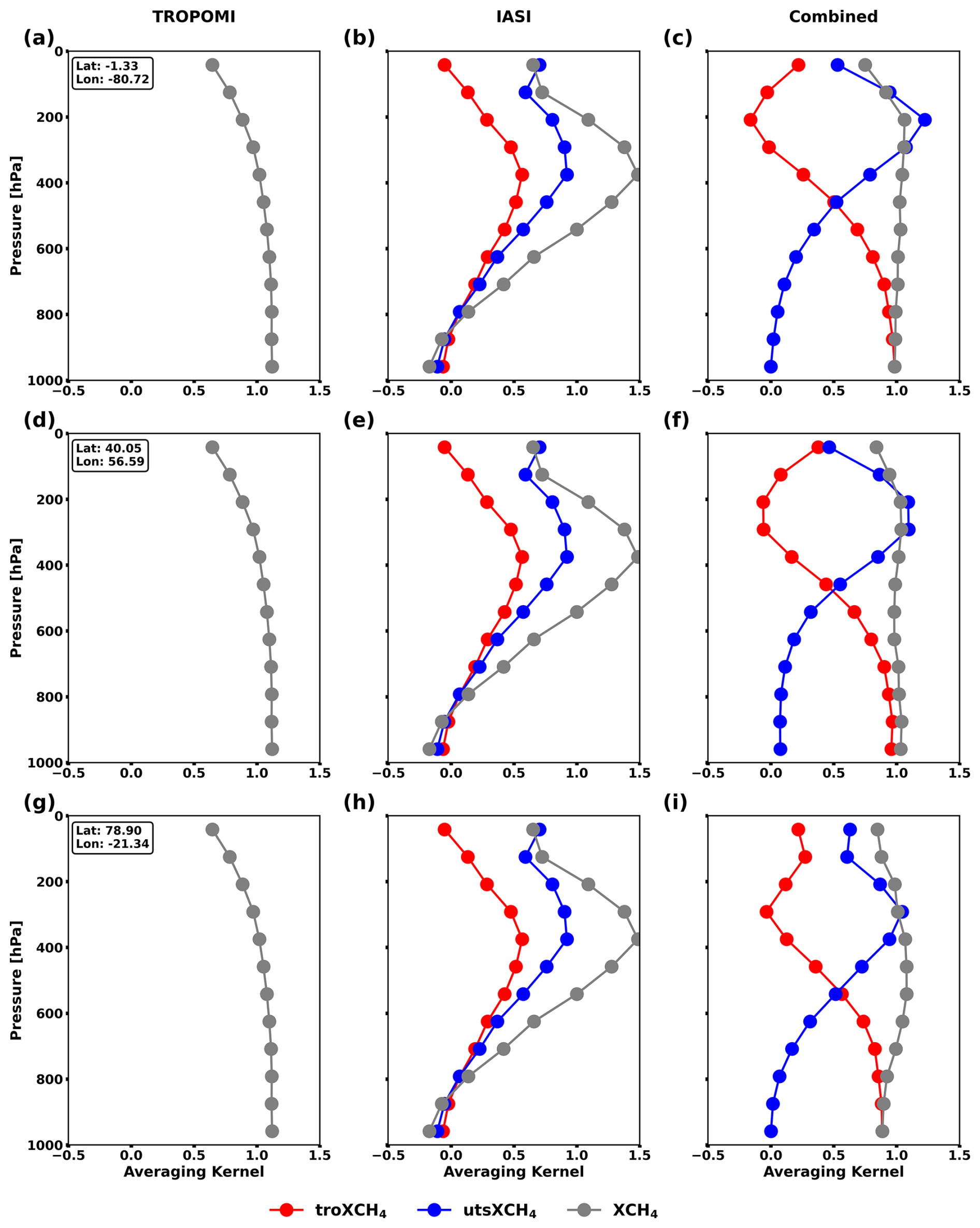
Figure 5 Total and partial column amount kernels for TROPOMI (a, d, g), IASI (b, e, h), and the combined product (c, f, i). Grey: total column amount kernel (XCH₄); Blue: upper tropospheric and stratospheric partial column amount kernel (utsXCH₄); Red: tropospheric partial column amount kernel (troXCH₄). (a, b, c) Low latitude; (d, e, f) Middle latitude; (g, h, i) High latitude.

Figure 5a, d, g depict typical total column averaging kernels of TROPOMI (grey line and symbols) for an observation at low, middle, and high latitudes. The kernel values are close to 1.0, indicating the good sensitivity throughout the atmosphere and at the different latitudes.

In Fig. 5b, e, h, the IASI averaging kernels are shown (grey for the total column, blue for the upper troposphere and stratosphere, and red for the troposphere). The IASI XCH₄ product is mainly sensitive to CH₄ between 650 and 100 hPa (total column averaging kernel values between 0.5 and 1.5, grey colour). IASI has a rather limited sensitivity above 650 hPa and the sensitivity is rather poor close to the surface (total column averaging kernel values are very close to zero, grey colour). IASI is well-suited for measuring the upper tropospheric and stratospheric CH₄ concentrations. The respective averaging kernel (blue colour) has largest values for the altitudes between 500 and 100 hPa. The missing sensitivity of IASI for surface-near CH₄ is illustrated by the tropospheric averaging kernel (red colour), whose values are below 0.3 for all pressures above 700 hPa.

The averaging kernels of the combined product are depicted in Fig. 5c, f, i. The total column averaging kernels of the combined product (grey colour) and the individual TROPOMI product are very similar, indicating that almost all information needed for detecting XCH₄ is provided by TROPOMI, and IASI only contributes weakly with additional information. Concerning the upper troposphere and stratosphere, the averaging kernel of the combined product (blue colour) is very similar to the IASI averaging kernel, indicating in turn that the information for detecting utsXCH₄ comes from IASI and TROPOMI adds only a very small amount of additional information. The partial column kernel representing the combined troXCH₄ product (red colour) is significantly different from the respective IASI averaging kernel. It has high values (between 0.8 and 1.0) from the surface up to about 700 hPa and low values for the upper troposphere/stratosphere (for pressures below 450 hPa the values are below 0.4). This documents that the combined troXCH₄ data product is well sensitive to CH₄ variations in the surface-near troposphere and furthermore, it is not significantly affected by CH₄ variations that may occur in the upper troposphere and stratosphere. The combined data product is superior to the individual TROPOMI and IASI data products: the XCH₄ and utsXCH₄ data of the combined product are as representative for total column averages and partial upper tropospheric and stratospheric column averages as the respective TROPOMI and IASI data products. However, only the combined product offers useful troXCH₄ data (TROPOMI or IASI alone cannot detect the tropospheric CH₄).

In the sections and figures of the remainder of this paper, we focus on the discussion of the data characteristics of the combined products. For XCH₄, the data characteristics are similar to the respective TROPOMI product, for utsXCH₄ they are similar to the respective IASI product, and for troXCH₄ they are exclusive for the combined product.

4.3 Global sensitivity patterns

As a measure for the sensitivity, we use the vertical profile averaging kernel matrix and calculate the sum of the diagonal elements of the vertical layers represented by XCH₄ (all vertical layers, i.e. we calculate the trace of the full matrix), the vertical layers represented by utsXCH₄ (50 % uppermost layers of the atmosphere), and the vertical layers represented by troXCH₄ (50 % lowermost layers of the atmosphere). In the following, we refer to these sums of the diagonal elements of the averaging kernels as the degree of freedom for signal (DOFS).

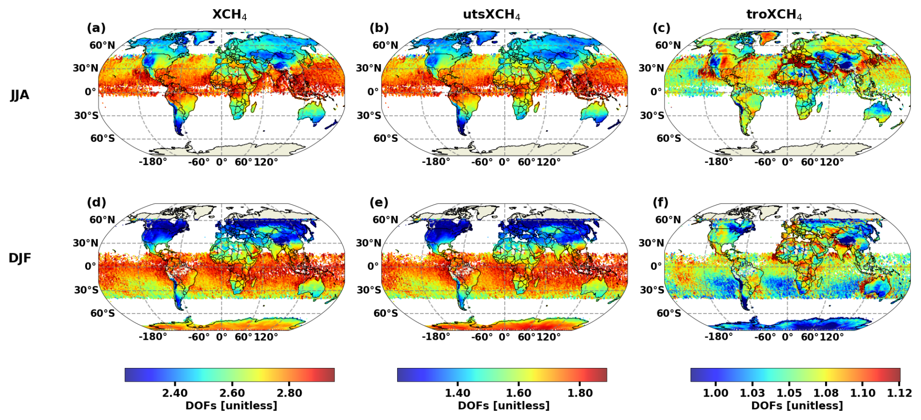
Figure 6 Degree of Freedom of Signal (DOFS) of the combined products averaged for 50 km × 50 km grid boxes. For the total column (XCH₄, a, d), the upper troposphere and lower stratosphere (utsXCH₄, b, e), and the troposphere (troXCH₄, c, f). (a, b, c) June, July, and August; (d, e, f) December, January, and February.

Figure 6 shows global maps of 50 km × 50 km averages of DOFS values for JJA and DJF. Figure 6a, d shows the DOFS values for the XCH₄ data product. Please note that with calculations according to Eq. (3), we get a combined profile product and the respective mixing ratio profile averaging kernels can be calculated according to Eq. (8). From this mixing ratio profile averaging kernel, we calculate the DOFS of the combined XCH₄ product. It is is typically 2–3 and shows a latitudinal dependency. It is largest at low latitudes and lowest at middle/high latitudes of the winter hemisphere.

Figure 6b, e depicts the averaged DOFS values for the utsXCH₄ data product. The DOFS values are typically between 1.2 and 2.0, and there is also a clear latitudinal dependence. As for the XCH₄ data product, we observe highest values at low latitudes and lowest values at high latitudes of the winter hemisphere.

The latitudinal gradients in the XCH₄ and utsXCH₄ DOFS follow respective DOFS gradients in the IASI profile data. This gradients are due to the IASI retrieval CH₄ a priori constraint, which is weaker around the tropopause (if compared to the free troposphere below the tropopause), because of an assumed high CH₄ variabilities in upper troposphere and stratosphere caused by a priori uncertainties of the tropopause altitude. Since the tropopause altitude is lower at high latitudes than at low latitudes, the overall IASI constraints are weaker over high latitudes if compared to low latitudes, which in turn gives higher DOFS values.

The troXCH₄ DOFS values are illustrated in Fig. 6c, f. They are weakly above 1.0 for almost all locations around the globe. This confirms the good sensitivity of the combined troXCH₄ product to actual CH₄ variations taking place in the lowermost 50 % of the atmosphere.

4.4 Response on surface-near and upper tropospheric/stratospheric CH₄

In order to demonstrate the capacity of the combined data product for detecting surface-near CH₄ independently from upper tropospheric/stratospheric CH₄ on global scale, we perform an extensive sensitivity study. We simulate CH₄ disturbances caused by uncertainties of the tropopause altitude (we assume a ±33 % uncertainty of the tropopause pressure). The CH₄ signals from such tropopause uncertainties hamper the investigation of boundary layer CH₄ fluxes and should be as small as possible. In addition, we examine atmospheric CH₄ changes by incrementing boundary layer CH₄ by 10 %. The accurate observation of this surface-near CH₄ variation is best-suited for surface-near CH₄ flux estimations. Appendix C shows an example of how the tropopause uncertainty and the boundary layer CH₄ increment affect the vertical CH₄ distribution and the total and partial column-averaged mixing ratio values.

The response ($\mathrm{\Delta }{\widehat{x}}^{*}$) of the XCH₄, utsXCH₄, and troXCH₄ data products on these atmospheric CH₄ disturbances (mixing ratio disturbance profiles Δx) can be calculated according to:

$$\begin{array}{}\text{(10)}& \mathrm{\Delta }{\widehat{x}}^{*}={\mathit{a}}^{*}{}^{\mathrm{T}}\mathrm{\Delta }\mathit{x}.\end{array}$$

Here a^*T are the total or partial column-averaged mixing ratio kernels (for XCH₄, utsXCH₄, or troXCH₄, respectively). The column-averaged mixing ratio kernels can be calculated from the column amount kernels (a^T) according to Eq. (4), which shows the corresponding calculation for the TROPOMI total column kernel.

Figures 7 and 8 show global maps of 50 km × 50 km averages of the responses for JJA and DJF, respectively. For both seasons we get very similar results: the XCH₄ product has a significant response on both disturbances, i.e. the tropopause shift and the boundary layer CH₄ increment. The response on the CH₄ boundary layer increment is observed at all locations equally well, but there is also a strong response on the tropopause shift. At high latitudes, the tropopause shift and the boundary layer increment cause signals of similar magnitudes. The utsXCH₄ product does not significantly respond on boundary layer CH₄ disturbances and it captures very well the CH₄ changes due to a shifted tropopause. The troXCH₄ product is not significantly affected by the CH₄ disturbances around the tropopause and captures very well the boundary layer CH₄ variations at any location. These Figs. 7 and 8 are very similar to Figs. C2 and C3, which demonstrates the good vertical sensitivity of the combined CH₄ product: the utsXCH₄ data are globally sensitivity on CH₄ changes around the tropopause and independent on boundary layer CH₄ changes. The troXCH₄ data in turn are globally sensitivity on boundary layer CH₄ changes and independent on CH₄ changes around the tropopause, thus very promising for CH₄ surface flux research.

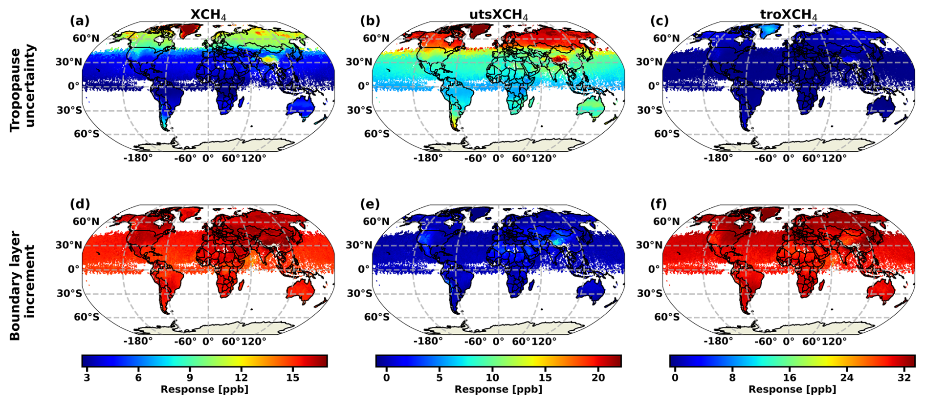
Figure 7 Response of the combined retrieval products on tropopause uncertainty and boundary layer CH₄ increment averaged for 50 km ×50 km grid boxes for June, July, and August (JJA). (a, b, c) Response on the tropopause uncertainty (±33 % up-/downward pressure shift of the climatological tropopause); (d, e, f) Response on a 10 % increment of CH₄ in the first layer above ground. The estimation are made according to Eq. (10) for (a, d) XCH₄; (b, e) utsXCH₄; (c, f) troXCH₄.

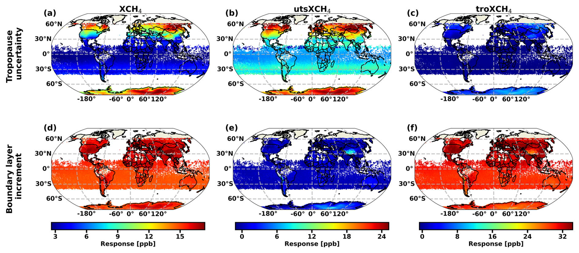
Figure 8 Same as Fig. 7, but for December, January and February (DJF).

5 Errors

In this section, we analyse the errors of the combined data products. We consider two kind of errors: the noise error caused by the measurement noise of the sensors and deficits in correctly modelling the spectra (e.g. due to insufficient knowledge of surface emissivity or albedo and spectroscopic line shapes or line intensities), and the dislocation error caused by spatial and temporal mismatches.

5.1 Noise error

According to Eq. (5) of Schneider et al. (2022b), the noise error covariances of the combined data product can be calculated from the noise errors of the TROPOMI data product (the variance $S_{\mathrm{T},n}^{*}$) and from the IASI noise error covariances (S_I,n):

$$\begin{array}{}\text{(11)}& {\mathbf{S}}_n=(\mathbf{I}-\mathit{g}{\mathit{a}}_{\mathrm{T}}^{*}{}^{\mathrm{T}}){\mathbf{S}}_{\mathrm{I},n}(\mathbf{I}-\mathit{g}{\mathit{a}}_{\mathrm{T}}^{*}{}^{\mathrm{T}}{)}^{\mathrm{T}}+\mathit{g}{S}_{\mathrm{T},n}^{*}{\mathit{g}}^{\mathrm{T}}.\end{array}$$

The error variance of a partial column-averaged mixing ratio state (S^*) can then be calculated from the covariance matrices that represent the errors of the mixing ratio profiles (S):

$$\begin{array}{}\text{(12)}& S^{*}={\mathit{w}}^{*}{}^{\mathrm{T}}\mathbf{S}{\mathit{w}}^{*},\end{array}$$

i.e. for calculating the noise error variances of the combined product, we use as S the noise covariance S_n of Eq. (11).

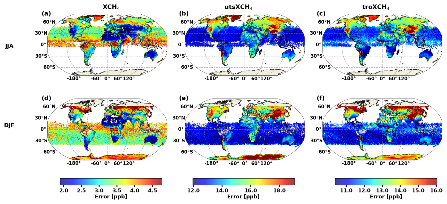
Figure 9 Noise error of the combined products averaged for 50 km × 50 km grid boxes. For the total column (XCH₄, a, d), the upper troposphere and lower stratosphere (utsXCH₄, b, e), and the troposphere (troXCH₄, c, f). (a, b, c) June, July, and August; (d, e, f) December, January, and February.

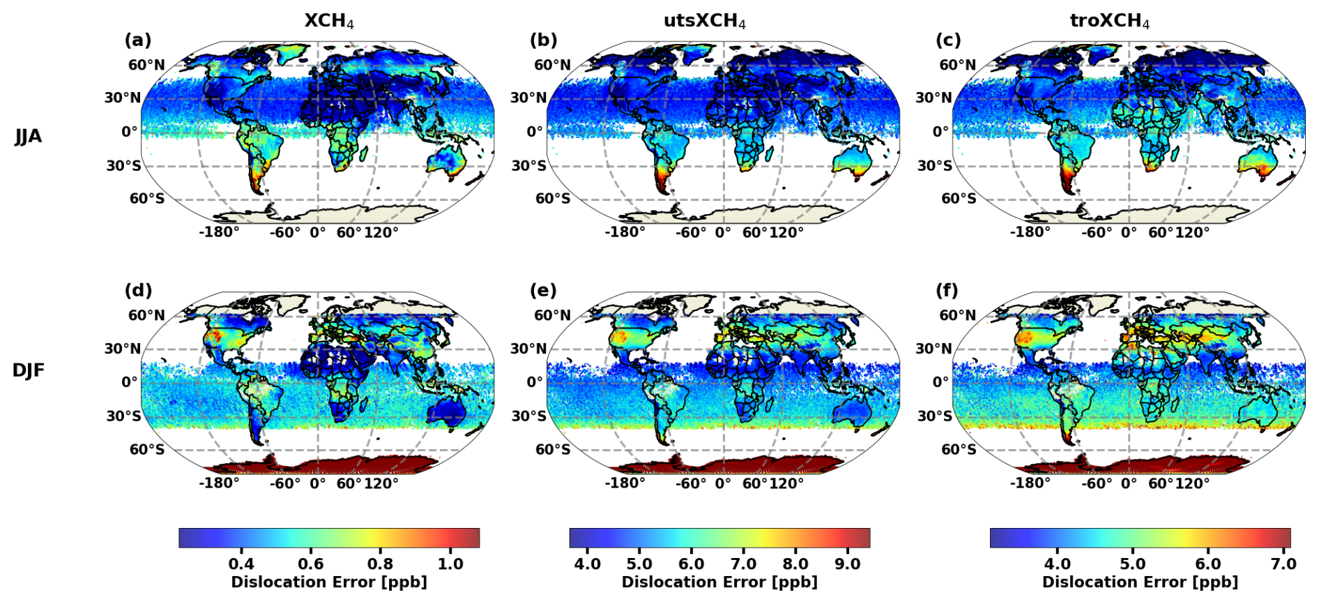
Figure 10 Same as Fig. 9, but for the dislocation error.

Figure 9 depicts 50×50 km averages for JJA and DJF of the noise error for the different data products (i.e. the square-root-values of the variances obtained according to Eq. 12). The XCH₄ product is mainly controlled by the TROPOMI L2 data and the observed error patterns largely follow the error patterns as given in the TROPOMI L2 data product. The utsXCH₄ product in turn is mainly controlled by the IASI L2 data. Consequently, the observed utsXCH₄ error pattern corresponds to the pattern of the IASI L2 errors. We observe highest noise errors for retrievals over cold surfaces (retrievals over high latitudes especially in the winter hemisphere and retrievals over high surface altitudes). This is typical for a thermal nadir sensor, and can be explained by a relative low signal to noise ratio over the corresponding areas (the intensity of the radiances that reach the satellite depend on the intensity of the randiances as emitted by the surface and the atmosphere). The troXCH₄ noise errors depend on TROPOMI and IASI noise errors. However, the IASI L2 noise errors are much larger than the TROPOMI L2 errors. As a result the troXCH₄ error patterns also follow largely the IASI L2 error patterns.

Concerning XCH₄, the noise error is smaller than 5 ppb, except for a few locations of winter hemispheric high/middle latitudes. The utsXCH₄ noise error is about 12 ppb over warm surfaces and up to 20 ppb over very cold surfaces (land with high surface elevations, e.g. Greenland, Himalaya, Andes, Antarctica). For troXCH₄, the noise error is about 10 ppb over warm surfaces and it can reach about 16 ppb over very cold surfaces.

5.2 Dislocation error

The dislocation error covariance matrix is calculated by

$$\begin{array}{}\text{(13)}& {\mathbf{S}}_{\mathrm{dl}}={\mathbf{A}}_{\mathrm{dl}}{\mathbf{S}}_{{\mathrm{\Delta }}_{\mathrm{dl}}}{\mathbf{A}}_{\mathrm{dl}}^{\mathrm{T}}\end{array}$$

where

$$\begin{array}{}\text{(14)}& {\mathbf{A}}_{\mathrm{dl}}=(\mathbf{I}-\mathit{g}{\mathit{a}}_{\mathrm{T}}^{*}{}^{\mathrm{T}}){\mathbf{A}}_{\mathrm{I}}\end{array}$$

is the dislocation averaging kernel and ${\mathbf{S}}_{{\mathrm{\Delta }}_{\mathrm{dl}}}$ is the covariance matrix for the CH₄ dislocation uncertainty. The dislocation uncertainty is determined from analysing the time and space variations of CAMS (Copernicus Atmospheric Monitoring Service) CH₄ forecast products at very high resolution (≈9 km; Barré et al., 2021). More details on the estimation of the dislocation uncertainty covariance are given in Appendix E of Schneider et al. (2022b).

From the dislocation error covariances (S_dl), we calculate the dislocation variances for the layers representing the XCH₄, utsXCH₄, and troXCH₄ data products according to Eq. (12). Figure 10a–f depicts the square-root-values of these variances in terms of averages for the JJA and DJF seasons. The dislocation error tends to be larger in the southern hemisphere than in the northern hemisphere, which reflects the latitudinal gradient of the temporal mismatch (see Fig. 3). Moreover, we observe that locations with high surface elevation (e.g., Rocky Mountains, Spain, Himalaya) have a more substantial dislocation error than the surrounding regions. This is caused by a higher surface pressure variation over complex terrain and consequently a lesser probability to find two horizontally close pixels with similar surface pressures. Overall, the dislocation errors are significantly smaller than the noise errors (compare Figs. 9 and 10).

6 The added value of troXCH₄

In the previous sections, we document the coverage and the characteristics of the data products. This section discusses the different patterns observable in the three data products: the XCH₄ and utsXCH₄ products, which have a similar characteristics as the respective individual TROPOMI XCH₄ and IASI utsXCH₄ products, and the troXCH₄ product, which is exclusively available in the combined data product (there is no respective TROPOMI or IASI data product). In the following, we illustrate the value that the troXCH₄ product adds to the XCH₄ and utsXCH₄ products.

6.1 Global CH₄ patterns

Figure 11 shows the JJA and DJF 50 km × 50 km averages for XCH₄, utsXCH₄ and troXCH₄. There is a systematic difference between the typical XCH₄, utsXCH₄ and troXCH₄ values. Typical values are 1750–1900 ppb for XCH₄, 1650-1875 ppb for utsXCH₄, and 1800–2000 ppb for troXCH₄. The decrease of the typical values, from troXCH₄ over XCH₄ to utsXCH₄, is caused by the decrease of the CH₄ concentrations above the tropopause, which is generally located at altitudes above the 300–400 hPa pressure level. The troXCH₄ product are the averaged mixing ratios for the lowermost 50 % of the atmosphere, i.e. a layer that is generally not affected by the CH₄ decrease at high altitudes. The total column averages (XCH₄) are partly affected by this decrease. The utsXCH₄ product represents the uppermost 50 % of the atmosphere, i.e. CH₄ mixing ratios at high altitudes, and it is strongly affected by the CH₄ decrease above the tropopause.

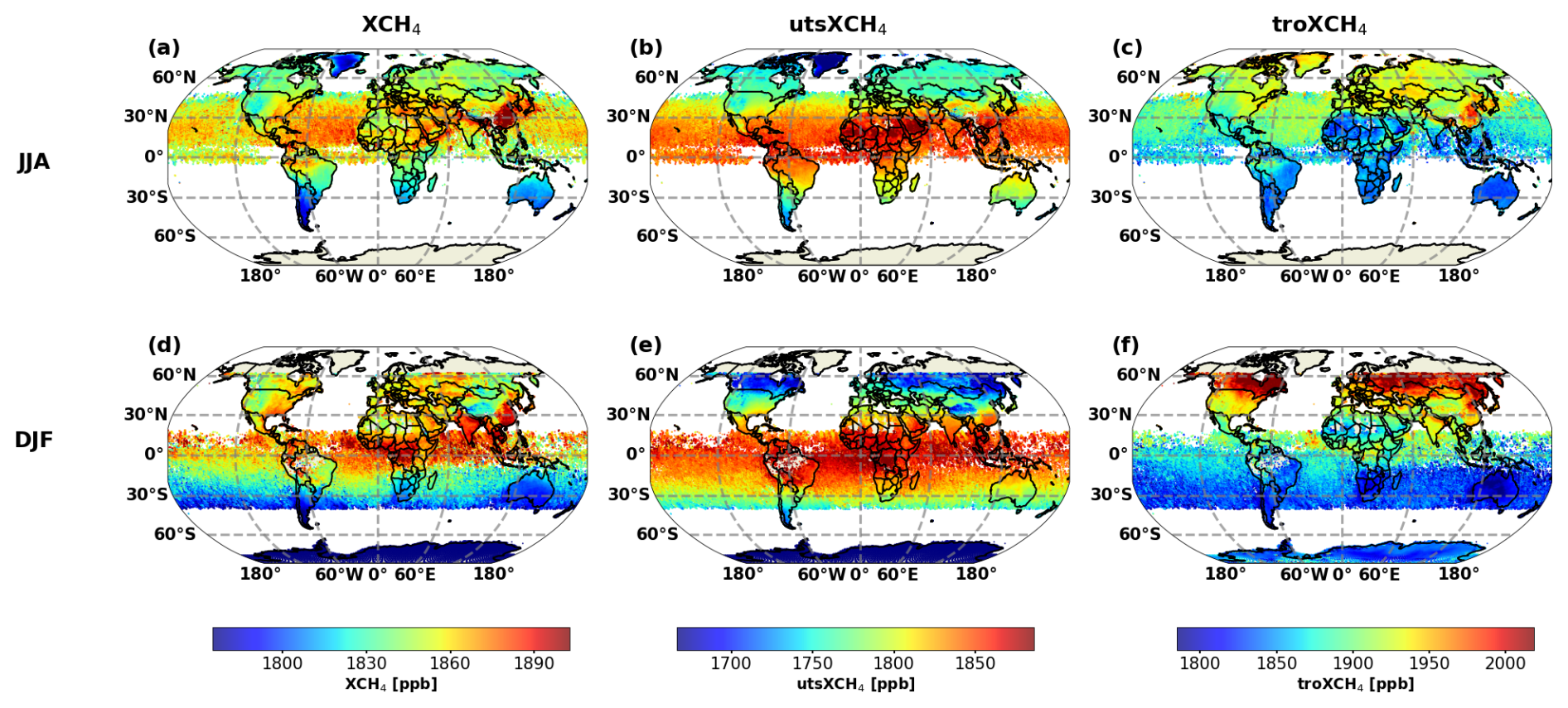
Figure 11 Global combined methane data products averaged for 50 km × 50 km grid boxes. For the total column (XCH₄, a, d), the upper troposphere and lower stratosphere (utsXCH₄, b, e), and the troposphere (troXCH₄, c, f). (a, b, c) June, July, and August; (d, e, f) December, January, and February.

The tropopause altitudes are lowest at high latitudes (around the 300–400 hPa pressure level) and highest in the tropics and subtropics (around the 100 hPa pressure level). This latitudinal gradient is mainly responsible for the gradients observed in the utsXCH₄ data (Fig. 11b, e). In the tropics and subtropics, where a large part of the uppermost 50 % of the atmosphere is situated below the tropopause, the utsXCH₄ values are rather high (1800–1900 hPa). Vice versa, at middle and high latitudes, a significant part of the uppermost 50 % of the atmosphere is above the tropopause and consequently the utsXCH₄ values are low (1600–1750 ppb).

As aforementioned, the troXCH₄ product is not significantly affected by the tropopause altitude, and consequently the horizontal patterns, as seen in the troXCH₄ maps (Fig. 11c, f) are significantly different from the utsXCH₄ patterns. For troXCH₄, we see a clear gradient with increasing values from the Southern to the Northern hemisphere. This gradient is most pronounced in the map showing the DJF averages (i.e. in the season when CH₄ concentrations peak in the Northern hemispheric troposphere, e.g. Frankenberg et al., 2005). Moreover, there are some troXCH₄ hotspots, i.e. locations where the mixing ratios are larger than in its surrounding (e.g. tropical Africa and tropical South America, Northern India, and North-Eastern China), which are areas with high natural and/or anthropogenic CH₄ emissions (e.g. Saunois et al., 2016). This suggests, that the global troXCH₄ patterns are directly related to global CH₄ emission patterns.

Mixing ratios averaged over the total column (i.e. the XCH₄ product) are impacted by lower tropospheric and tropopause altitude related CH₄ signals. This is evident in Fig. 11a, d, which demonstrates that the global pattern observed in the XCH₄ data product results from a superposition of the global tropopause altitude distribution and the global CH₄ emission pattern.

6.2 Local CH₄ time series

Figure 12 shows a time series for Madrid (39.42–41.42° N and 4.70–2.70° W) for January 2018 to June 2021 of the combined data products. The first row shows the combined methane products (XCH₄, utsXCH₄, and troXCH₄, Fig. 12a–c). The utsXCH₄ time series shows the strongest seasonal cycle, with a maximum during the end of summer/autumn and a minimum in winter/spring. This observation is explained by the respective seasonal cycle of the tropopause altitude (see also the discussion in the context of Fig. 11). Seasonal cycle signals are much weaker in the XCH₄ and troXCH₄ time series. The XCH₄ product is still weakly affected by the seasonal cycle of the tropopause altitude. It shows a maximum during the end of summer and autumn, but the minimum in winter/spring is hardly observable. This is due to the seasonal cycle of methane in the lower troposphere, being characterised by a maximum in winter/spring. This winter/spring maximum is actually the dominating seasonal cycle signal in the troXCH₄ time series (see Fig. 12c).

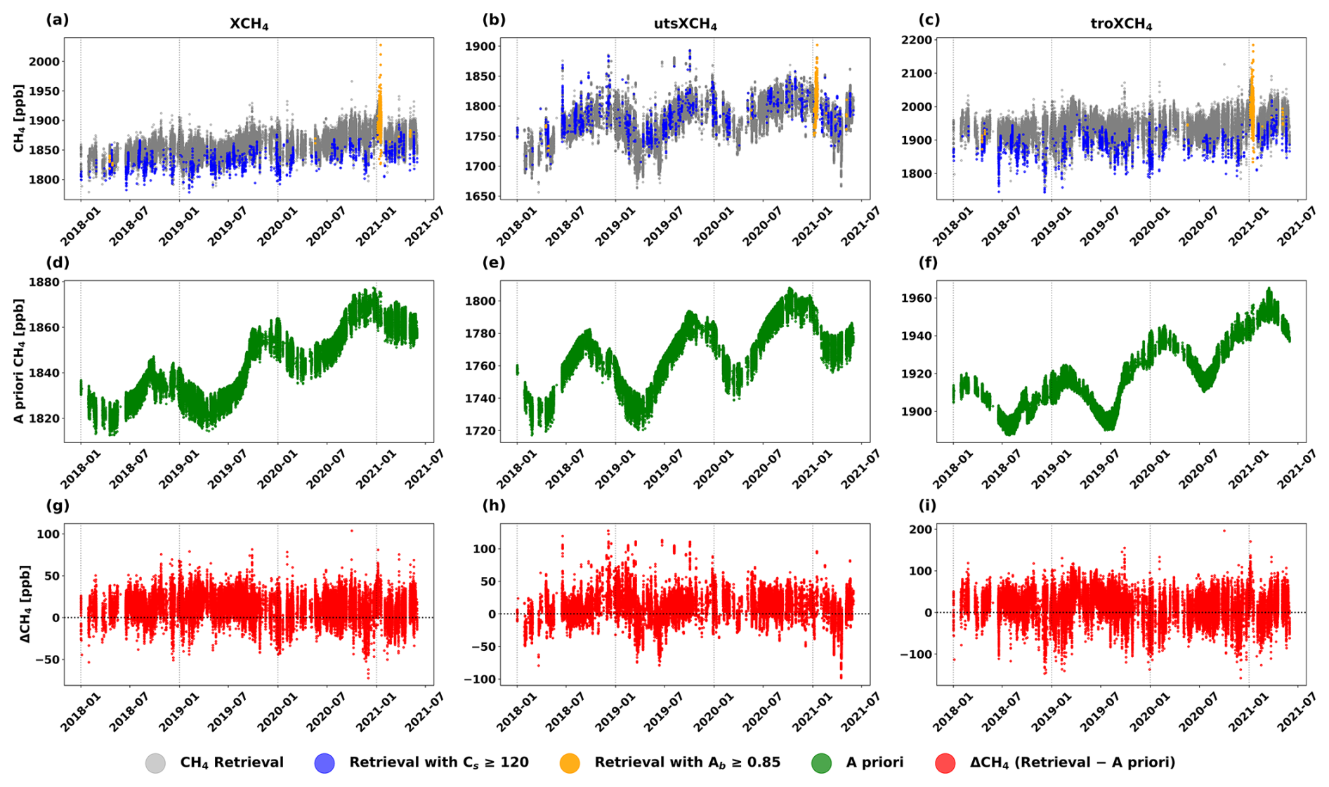
Figure 12 Time series data (January 2018–June 2021) for a 2°×2° area around Madrid. (a, b, c) Retrieved products (orange colour indicates data points where the blended albedo (A_b) ≥ 0.85, blue highlights where the TROPOMI aerosol parameter (C_s) ≥ 120, and grey represents all other data points); (d, e, f) The a priori data. (g, h, i) The difference between the retrieved and the a priori data. (a, d, g) XCH₄; (b, e, h) utsXCH₄; (c, f, i) troXCH₄.

In Fig. 12a–c, we mark data that might be affected by higher TROPOMI uncertainties, due to a snow covered surface (data marked by orange colour) or due to strong aerosol scattering (data marked by blue colour). Lorente et al. (2021) documents larger TROPOMI XCH₄ uncertainties for observations over ground covered by snow. These observations can be identified by the so-called blended albedo (A_b) being larger than 0.85 (Wunch et al., 2011b):

$$\begin{array}{}\text{(15)}& A_{\mathrm{b}}=\mathrm{2.4}{A}_{\mathrm{NIR}}-\mathrm{1.13}{A}_{\mathrm{SWIR}}.\end{array}$$

Furthermore, scattering by aerosols and cirrus particles can cause high errors in the TROPOMI XCH4 product if not appropriately taken into account. Butz et al. (2012) introduced the parameter

$$\begin{array}{}\text{(16)}& C_{\mathrm{s}}={\displaystyle \frac{{\mathit{\tau }}_{\mathrm{s}}{z}_{\mathrm{s}}}{{\mathit{\alpha }}_{\mathrm{s}}}},\end{array}$$

and suggests to filter out observations with C_s above 120 m, because of significant aerosol scattering and thus potentially large uncertainties in the TROPOMI XCH₄ product (τ_s, z_s, and α_s are estimated by the TROPOMI retrieval code and represent the optical aerosol thickness, the centre height of the aerosol layer, and the aerosol size parameter, respectively).

Figure 12d–f shows the a priori data simulated by the TM5 model. The a priori data show much less small scale variability than the retrieved data and enable a clear identification of the different seasonal cycles in the troposphere and the upper troposphere/stratosphere.

Figure 12g–i shows the difference of the retrieved values and the a priori data ($\mathrm{\Delta }{\mathrm{CH}}_{\mathrm{4}}={\mathrm{CH}}_{\mathrm{4}}-\mathrm{Apriori}{\mathrm{CH}}_{\mathrm{4}}$). The data that might be affected by snow covered surface or strong aerosol scattering have been filtered out. The large scatter indicates that on small scales the a priori model can differ significantly from the observations. Since these differences are significantly larger than the uncertainties of the observations, the observations seem to provide a lot of information about small-scale processes that is not captured by the TM5 a priori model. In particular in the utsXCH₄ and troXCH₄ time series, we can also observe signals on a seasonal scale, that are beyond the uncertainties of the observations. This suggests that the observations contain also information about large-scale processes that are not captured by the model. In this context, the separation into utsXCH₄ and troXCH₄ gives valuable additional information. For instance, in the beginning of 2019 the ΔCH₄ values for the upper troposphere/stratosphere and the troposphere differ systematically from zero, but they are not correlated, i.e. this discrepancy between model and observations is less visible in the XCH₄ data and can be much better identified in the combined utsXCH₄ and troXCH₄ products.

6.3 Regional CH₄ patterns

Figure 13a–c depicts the 3.5 year average (January 2018–June 2021) of XCH₄, utsXCH₄, and troXCH₄ on a 0.1°×0.1° grid with a zoom on the Iberian Peninsula and Fig. 13d shows a respective map of the EDGAR v7.0 anthropogenic emissions catalogue (representative for 1970–2022, Crippa et al., 2024). We only plot the XCH₄, utsXCH₄, and troXCH₄ averages when at least 10 individual observations are availble for the respective 0.1°×0.1° grid box, which largely explains the locations with no data in Fig. 13a–c. This area has also been used in Tu et al. (2022) for studying landfill methane emission from ground and space.

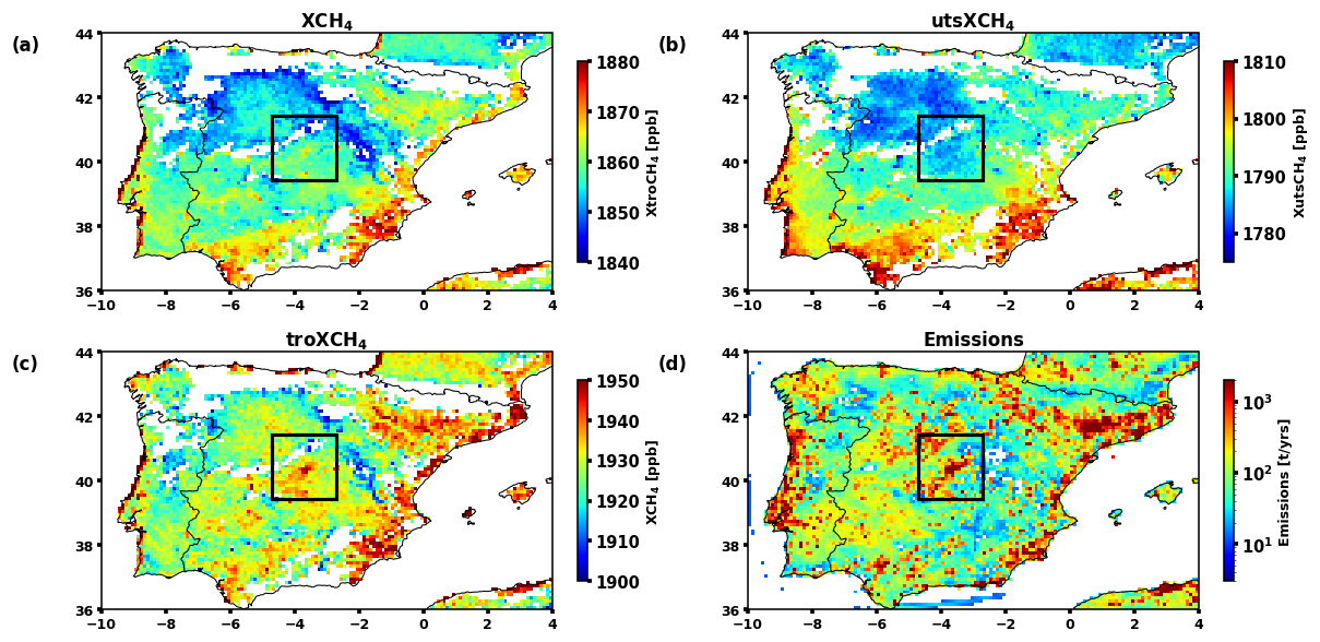
Figure 13 Methane concentration obtained from the combined product (January 2018–June 2021) and anthropogenic emission data (1970–2022) averaged for 0.1°×0.1° grid boxes for the Iberian Peninsula. (a) XCH₄; (b) utsXCH₄; (c) troXCH₄; (d) anthropogenic emissions of EDGAR v8.0 GHG. The black box indicates the 2°×2° area around Madrid used in the context of Fig. 12.

Concerning the XCH₄ and utsXCH₄ maps, we observe a clear north-south gradient. In the northern part of the Peninsula, XCH₄ is generally below and in the southern part above 1860 ppb. Similar for utsXCH₄, which is mainly below 1790 ppb in the north and above 1790 ppb in the south. Exceptions are the coast lines, and the Ebro valley (south of the Pyrenees), for which XCH₄ values are also occasionally above 1860 ppb in the north. The pronounced north-south gradient in the 3.5 year average is caused by the climatology of the tropopause altitude. Climatologically (average over 3.5 years) the tropopause is significantly lower (at higher pressure levels) in the north than in the south.

The horizontal patterns of the troXCH₄ map are significantly different from the patterns in the respective XCH₄ and utsXCH₄ maps. We do not observe a significant north-south gradient. The atmospheric layer represented by troXCH₄ is below the tropopause, even for extreme cases when it might be situated at 300–400 hPa. Consequently, the troXCH₄ values are independent from the strong CH₄ signals introduced by the location of the tropopause. We observe highest troXCH₄ values (above 1940 ppb) in the Ebro valley, in the center of the Peninsula in the area around Madrid, and along the coast lines. These troXCH₄ patterns are similar to the patterns present in the map of the anthropogenic EDGAR emissions inventories (Fig. 13d). This is a strong indication that the troXCH₄ product (only obtained by combining TROPOMI and IASI products) offers a much better possibility for monitoring the anthropogenic emissions than the XCH₄ and utsXCH₄ products, obtainable by TROPOMI and IASI alone.

7 Data quality recommendations

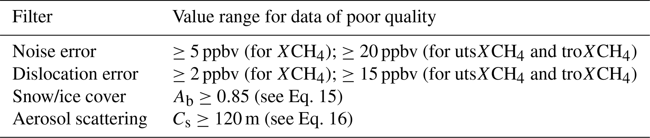
In this section, we give recommendation for filtering out data of reduced quality. We recommend filters for data that have an atypically large uncertainty caused by an atypically large noise of the original IASI and/or TROPOMI L2 data products or by a significant dislocation of IASI and TROPOMI (these errors are discussed in Sect. 5). Moreover, we recommend filters for data, where the TROPOMI observation might be strongly affected by surface snow cover and/or scattering by aerosols (these errors are discussed in Sect. 6.2).

For about 1 % of the all combined data, we estimate a noise error for XCH₄ of more than 5 ppbv and for utsXCH₄ and troXCH₄ of more than 20 ppbv. We recommend to use these values as thresholds for filtering out data of particularly poor quality. The dislocation error is significantly smaller, but can also affect the data quality. For about 1 % of all the combined data products, we estimate a dislocation error for XCH₄ of more than 2 ppbv and for utsXCH₄ and troXCH₄ of more than 15 ppbv. In order to avoid a significant impact of the dislocation error, we recommend to remove the respective data.

In Sect. 6.2, we introduce the blended albedo (A_b) and the aerosol parameter (C_s) for identifying TROPOMI data that might be significantly affected by surface snow cover and/or scattering by aerosols. In order to avoid an impact of these uncertainities on the combined data products, it is recommended to filter out data with A_b≥0.85 and with C_s≥120 m. Figure 14 illustrates the percentage of data rejection by these snow cover and aerosol scattering filters for the JJA and DJF seasons. The data rejections due to strong aerosol scattering is most prominent in the JJA season in the subtropics in North Africa, Southern Europe and Asia (Fig. 14a). These are the (semi-)desert areas which suggest that mineral dust aerosols can importantly impact on the TROPOMI data quality. The data rejection due to snow covered surfaces is very important over the polar regions and over the northern hemispheric middle latitudes in winter (DJF season, Fig. 14d). The quality filter recommendations are resumed in Table 2.

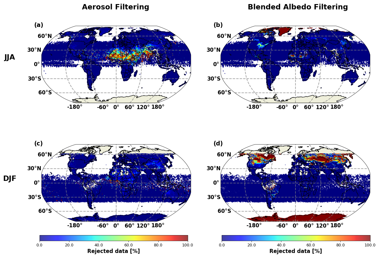
Figure 14 Relative number of data rejected per 50 km × 50 km grid boxes by the aerosol scattering filter (a, c) and the snow coverage filter (b, d). (a, b) June, July, and August; (c, d) December, January, and February.

Table 2 Table summarizing the recommendations for filtering out data of relatively poor quality. Data corresponding to here given value range should be filtered out for ensuring highest data quality.

8 Data availability

The here presented combined data set is referenced to https://doi.org/10.35097/wq583rnzpmd83m5g (Shahzadi et al., 2026) and also freely-accessible on our servers at KIT: https://www.imk-asf.kit.edu/english/CH4-synergy-IASI-TROPOMI_RemoTeC.php (last access: 8 March 2026). The here used MUSICA IASI data are described in Schneider et al. (2022a) and can be accessed at https://doi.org/10.35097/408 (Schneider et al., 2021) or downloaded at: https://www.imkasf.kit.edu/english/musica-iasi-v321.php (last access: 8 March 2026). The here used TROPOMI data are described in Lorente et al. (2023a) and available for download at https://doi.org/10.5281/zenodo.7766558 (Lorente et al., 2023b) or https://ftp.sron.nl/open-access-data-2/TROPOMI/tropomi/ch4/19_446/ (last access: 8 March 2026).

9 Summary

We apply the Schneider et al. (2022b) synergetic data combination method to the large TROPOMI and IASI CH₄ data sets. We generate a combined data set consisting of about 289 million data points, that are globally distributed and representative for the 42 month between January 2018 and June 2021. The combined data set consists of three different data products: total column-averaged mixing ratios (XCH₄), upper tropospheric and stratospheric column-averaged mixing ratios (utsXCH₄), and tropospheric column-averaged mixing ratios (troXCH₄). Whereas the former two have a very similar characteristics and quality as the respective TROPOMI and IASI data products, the latter is a unique outcome of the synergetic combination. High-quality and reliable troXCH₄ data can only be achieved by combining the two data sets optimally. This data product is neither available from TROPOMI nor from IASI alone.

We show that this troXCH₄ data product has a scientific impact on top of the XCH₄ and utsXCH₄ data products. While XCH₄ and utsXCH₄ are significantly affected by the strong CH₄ variations in upper troposphere and stratosphere (for instance, due to variations in the tropopause altitude), the troXCH₄ data product is strongly connected to the surface CH₄ emissions. Thus it offers important advantages over the individual TROPOMI and the IASI data products when it comes to the research and monitoring of anthropogenic CH₄ emissions.

The merged data set is available in the form of one NetCDF file per day of observation. The NetCDF data files comply with the FAIR principles (Wilkinson et al., 2016), i.e. among others, each data point is provided with its respective error and averaging kernel. Examples of data files and a README.pdf file informing users about access to the full data set are provided via https://doi.org/10.35097/wq583rnzpmd83m5g (Shahzadi et al., 2026). The full data set is made freely available at https://www.imk-asf.kit.edu/english/CH4-synergy-IASI-TROPOMI_RemoTeC.php (last access: 8 March 2026).

The method can easily be applied to other TROPOMI and IASI data sets, as long as these data are made available under consideration of the FAIR principles (the availability of individual errors and averaging kernels is mandatory). Moreover, the computational efficiency and flexibility of the method (automatic benefit from novel developments made by dedicated TROPOMI and IASI retrieval experts) will become important, particularly in the context of the Metop-SG (Second Generation) satellite mission (https://www.eumetsat.int/metop-sg, last access: 8 March 2026). Metop-SG has TROPOMI and IASI successor instruments aboard and offers an unprecedented high number of diverse and high-quality CH₄ data that can be used for a synergetic data combination.

Appendix A: Kalman gains

Figure A1 shows typical Kalman gain vectors g for low, middle, and high latitudes. The Kalman gain describes how discrepancies between the IASI L2 profile retrieval and the TROPOMI L2 total column data impact on the combined profile data product. This impact is generally largest close to ground where the IASI data product has the highest uncertainty (IASI has only limited sensitivity close to ground). At the lowermost layer a +1 ppb discrepancy between the TROPOMI and IASI L2 total column-averaged mixing ratios will change the background CH₄ mixing ratio profile (the IASI L2 profile) by about +3 ppm. On the other hand the impact is generally within ±1 ppm in the upper troposphere and stratosphere where the IASI data product has a low uncertainty (at the corresponding altitudes IASI has a reasonable sensitivity).

Figure A1 Kalman gain profiles obtained according to Eq. (5) for different latitudes: (a) low latitude; (b) middle latitude; (c) and high latitude. The results are shown for the same observations as used in Figs. 5 and B1.

Appendix B: Vertical profile kernels

The MUSICA IASI L2 CH₄ mixing ratio profiles are made available with mixing ratio profile averaging kernels and adding the information of the TROPOMI L2 total column product to the IASI L2 profile data results in a mixing ratio profile (see Eq. 3) and mixing ratio profile averaging kernels (see Eq. 8). In this appendix we show typical IASI L2 mixing ratio profile averaging kernels and compare them to the mixing ratio profile averaging kernels obtained when adding the information of the TROPOMI L2 product. Figure B1 illustrates these kernels for typical observations at low, middle, and high latitudes.

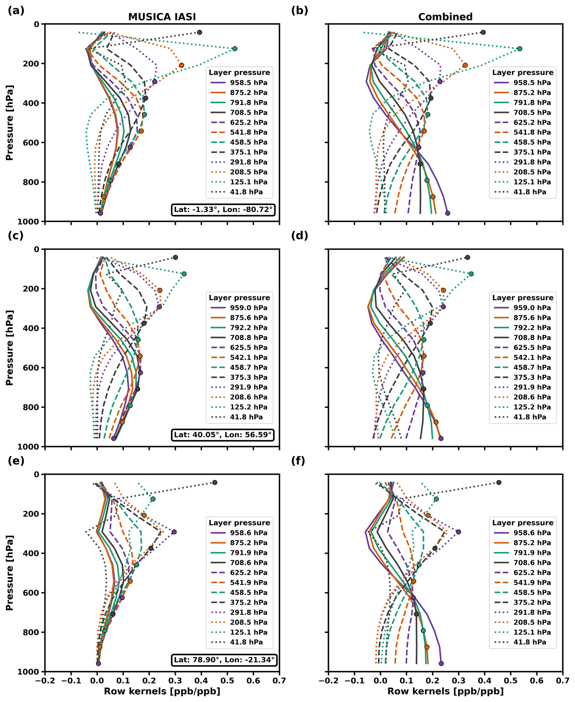
Figure B1 Volume mixing ratio profile row kernels for the MUSICA IASI L2 data product (a, c, e) and the combined data product (b, d, f) at different latitudes: (a, b) Low latitudes; (c, d) Middle latitudes; (e, f) High latitudes (e, f). The results are shown for the same observations as used in Figs. 5 and A1.

The IASI kernels reveal a good sensitivity in the upper troposphere and stratosphere, e.g. below 650 hPa the maximum kernel value is close to the pressure range represented by the kernel. However, in the lower troposphere the sensitivity is limited and the kernel values are small, e.g. for the first layer above ground this value is generally smaller than 0.05. The kernels of the combined product are very similar to the IASI kernels for the upper troposphere and stratosphere, revealing the good sensitivity at these layers. In the lower troposphere the kernels of the combined product show a much better sensitivity than the respective IASI kernels, e.g. the kernel value for the first layer above ground is generally about 0.25, which demonstraes that improved sensitivity with respect to surface-near CH₄ variations.

Appendix C: Sensitivity study

For our sensitivity study, we investigate how two different kinds of atmospheric CH₄ disturbances impact on the different products: (1) disturbances of CH₄ caused by shifting the tropopause to 33 % higher and lower pressure levels, and (2) disturbances of CH₄ by incrementing the CH₄ concentration in the first layer above ground by 10 %. The disturbances are made with respect to the CH₄ a priori profile. The disturbance Δx used in Eq. (10) are calculated as follows: for the tropopause shift disturbance we use $\mathrm{\Delta }\mathit{x}=\frac{\mathrm{1}}{\mathrm{2}}({\mathit{x}}_{\mathrm{up}}-{\mathit{x}}_{\mathrm{dn}})$, where x_up and x_dn are the CH₄ profiles obtained by up- and downward shifting the tropopause (see Fig. C1a, red lines). For the boundary layer increment disturbance we use $\mathrm{\Delta }\mathit{x}={\mathit{x}}_{\mathrm{inc}}-{\mathit{x}}_{\mathrm{a}}$, where x_a and x_inc are the CH₄ a priori profile and the a priori profile with by 10 % increased CH₄ concentrations in the first layer above ground (x_inc is shown as blue line in Fig. C1b).

The tropopause uncertainty and the boundary layer increment impact on the total and partial column-averaged mixing ratios. These impacts can be calculated by

$$\begin{array}{}\text{(C1)}& \mathrm{\Delta }{x}^{*}={\mathit{w}}^{*}{}^{\mathrm{T}}\mathrm{\Delta }\mathit{x},\end{array}$$

where w^*T is the the pressure weighted resampling operator (see Eq. 7) for the total, the tropospheric, and the upper tropospheric and stratospheric column. Figures C2 and C3 illustrate 50 km×50 km averages of these impacts for the JJA and the DJF seasons, respectively. Naturally, the tropospheric partial column (troXCH₄) is only impacted by increments of the boundary layer CH₄ levels. The impact on troXCH₄ is rather uniform and about 30 ppb (it is independent on locations and season). In turn, the upper tropospheric and stratospheric partial column (utsXCH₄) is only affected by the tropopause uncertainty. The respective impact is in particular large at high winter latitudes, where the tropopause pressure is high and consequently changes of the tropopause pressure affect larger airmasses than at low latitudes. The total column average (XCH₄) is significantly impacted by the tropopause uncertainties as well as the boundary layer CH₄ increment. For low winter latitudes, the impact of the tropopause uncertainty on XCH₄ is up to 15 ppb, which is very similar to the impact achieved for a 10 % increment of the boundary layer CH₄ concentrations.

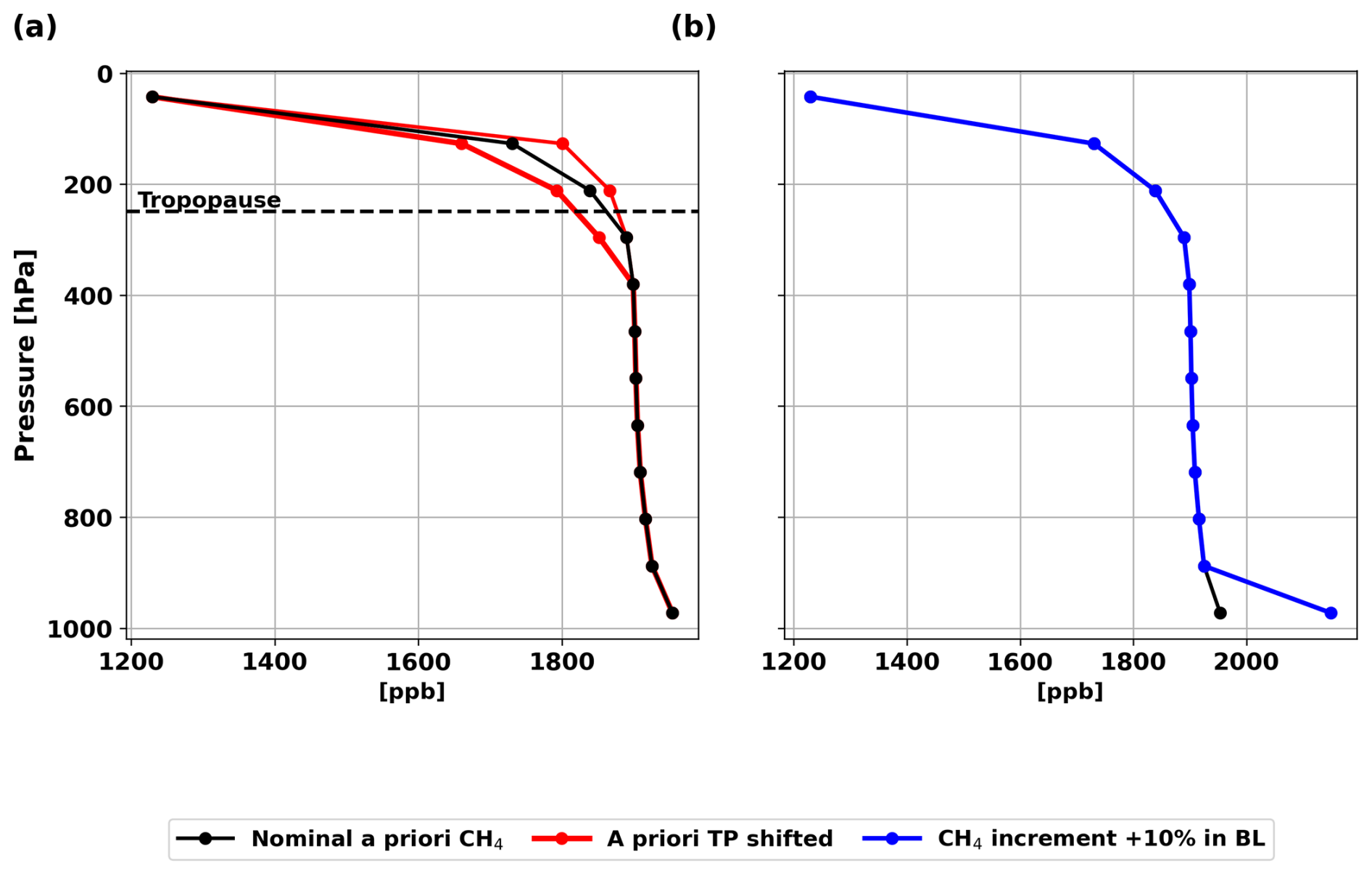
Figure C1 Atmospheric CH₄ disturbances used in our sensitivity study for a typical middle latitude observation (the disturbances are made with respect to the a priori profile, x_a, black line). (a) CH₄ profiles due to shifting the tropopause by ±33 % with respect to the climatological tropopause pressure (up-/downward, x_up and x_dn, red lines); (b): CH₄ profile due to incrementing the CH₄ concentrations by 10 % in the first layer above ground (x_inc, blue line).

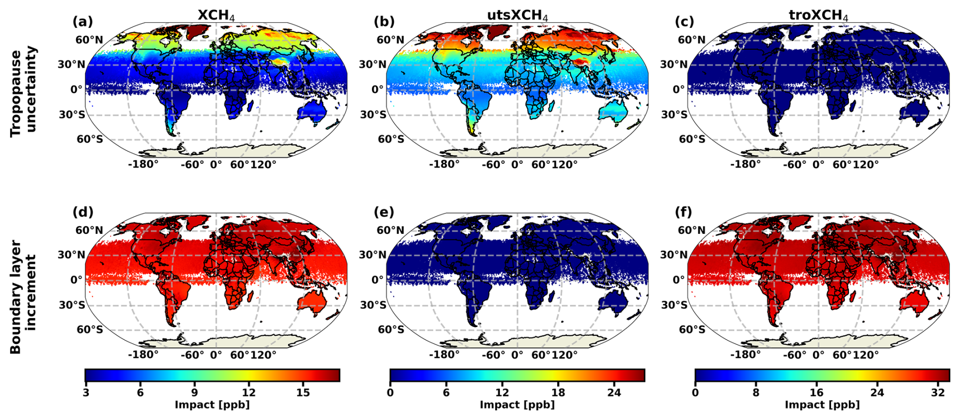
Figure C2 Impact of tropopause uncertainty and boundary layer CH₄ increment averaged for 50 km × 50 km grid boxes for June, July, and August (JJA). (a, b, c) Impact of a tropopause uncertainty (±33 % up-/downward pressure shift of the climatological tropopause); (d, e, f) Impact of a 10 % increment of CH₄ in the first layer above ground. The estimation are made according to Eq. (C1) for (a, d) XCH₄; (b, e) utsXCH₄; (c, f) troXCH₄.

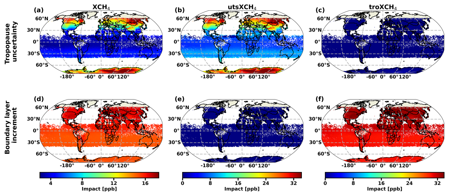
Figure C3 Same as Fig. C2, but for December, January and February (DJF).