CLIMATHUNDERR: experimental database of buoyancy-driven downbursts

Thunderstorm downbursts are windstorms due to intense negatively-buoyant flows produced beneath cumulonimbus clouds. Their study has recently attracted significant scientific and media attention due to the current and projected impacts of climate change. During their vertical descent phase (i.e., the downdraft), followed by a horizontal outflow, downbursts can cause severe damage to both natural ecosystems and built environments. The parent thunderstorm originates when warm, humid air is lifted upward through natural or forced convective mechanisms, where it condenses into a cumulonimbus cloud. Inside the cloud, the air parcels – now colder and denser than the surrounding environment – sink due to negative buoyancy. Thermal and dynamic instabilities between the cold air jet and the environment generate vortical structures. The first to form is known as the primary vortex, which drives both the downdraft and the subsequent horizontal outflow at the surface. This vortex flow structure can have devastating effects on the ground.

Building on these insights, a series of experiments was recently conducted as part of the CLIMATHUNDERR project – CLIMAtic Investigation of THUNDERstorm Winds – funded by the European Union through the European Research Infrastructures for European Synergies (ERIES) project. For the first time, the buoyancy effects that drive downdraft winds to the surface were reproduced at large fluid-dynamics geometric scales at the Jules Verne Climatic Wind Tunnel – Thermal Unit SC2 at the Centre Scientifique et Technique du Bâtiment (CSTB) in Nantes, France. This experimental campaign aimed to further explore thunderstorm wind phenomena, building on earlier research studies conducted at the WindEEE Dome in Canada under the European Research Council (ERC) Advanced Grant project THUNDERR. CLIMATHUNDERR extends this previous research by emphasizing thermal effects, which are key drivers in these wind events. In the experiments, downbursts were recreated using an upper plenum that simulates the thunderstorm cloud, innovatively combining two widely applied techniques: impinging jet and gravity current. Thermal effects were reproduced by controlling the temperature differential between the upper plenum and the air in the testing chamber. A mechanical piston controlled the outgoing flow velocity at the nozzle exit, simulating the contribution of a simple mechanical impinging jet. Benchmark experiments were performed with only the mechanical impinging jet, allowing the quantification of thermal effects at the interface between the jet and the calm surrounding air.

The experimentally generated downburst-like flows were then tested against a scaled orography model of the Polcevera Valley in Genoa, Italy, to examine how it influences the dynamics and structure of the downburst vortices.

Velocity measurements were performed using Particle Image Velocimetry (PIV), enabling a detailed reconstruction of the 2D vector flow field without the limitations of traditional anemometric instruments like multi-hole pressure probes, which struggle with low-velocity (i.e., <2 m s⁻¹) and reversal flows. Additionally, temperature profiles before and during downburst occurrence were measured with thermocouples distributed across the flow field.

This project draws on a multi-disciplinary team of experts in thunderstorm phenomena, facilitating a comprehensive analysis of the collected data from various perspectives, including data interpretation, atmospheric and meteorological insights, numerical simulations, and analytical methods. The experimental data are openly available to the scientific community via the Zenodo repository (https://doi.org/10.5281/zenodo.14609848, Canepa et al., 2025a).

1 Introduction

In recent decades, significant efforts in wind engineering and atmospheric sciences have focused on non-stationary wind phenomena caused by extreme weather events. The projected increase in frequency and intensity of such events, driven by climate change, has been widely discussed in recent studies (e.g., Allen, 2018; Bevacqua et al., 2019; Faranda et al., 2022; Prein, 2023; Púčik et al., 2017; Rädler et al., 2019; Taszarek et al., 2019, 2020). Among these, thunderstorm-generated winds, such as downbursts and tornadoes, pose considerable hazards, especially to mid-latitude regions. Severe winds, heavy rainfall, and hail associated with thunderstorms are frequently reported in the media, raising awareness even among non-specialists about the dangers of these phenomena. This heightened attention is driven by the destructive impacts of thunderstorms, which can result in loss of life, injuries, structural damage or collapse, and significant harm to the environment, society, and economy (Brooks, 2013; Allen, 2018). When thunderstorms produce multiple hazards – such as strong winds and hail simultaneously – addressing them through a multi-hazard approach has become a rapidly growing research area in environmental sciences and structural engineering (Forzieri et al., 2016; Gallina et al., 2016; Giachetti et al., 2021; Leinonen et al., 2023; Sadegh et al., 2018).

A thunderstorm downburst develops as air is dragged downward by falling raindrops and ice particles descending from a thunderstorm cloud, where precipitation loading influences the vertical velocity of the flow. The evaporation of these hydrometeors cools the descending air, increasing its density and thereby accelerating its downward motion under gravity. While most downbursts are associated with thunderstorms containing precipitation (so-called wet downbursts), dry downbursts can also occur when the descending air mass originates in a high-based convective cloud, with precipitation evaporating completely before reaching the ground. In both cases, the resulting thermodynamic and kinematic instabilities at the interface between the vertical jet and the surrounding environment generate vortical structures that govern the downburst flow (Fig. 1). The leading and most intense of these is the primary vortex (PV) (Canepa et al., 2025b), responsible for the maximum horizontal velocity near the ground (Fujita, 1981; Wakimoto, 1982; Hjelmfelt, 1988; Canepa et al., 2020). Continuous shear between the descending jet and the ambient air produces subsequent vortices, termed trailing vortices (TVs), which form and shed at an approximately constant frequency (Canepa et al., 2023). Moreover, the interaction of the PV with the ground promotes separation and reattachment of the boundary layer beneath it. This confined region ahead of the PV entrains a secondary counter-rotating vortex (SV) (Canepa et al., 2022b), which has also been observed in several full-scale field campaigns (Sherman, 1987; Canepa et al., 2020; Romanic, 2021). Upon reaching the ground, the downdraft's momentum shifts from vertical to horizontal, creating intense radial winds near the surface, the so-called downburst outflow. Figure 1 presents a schematic illustrating the evolution of thunderstorm winds.

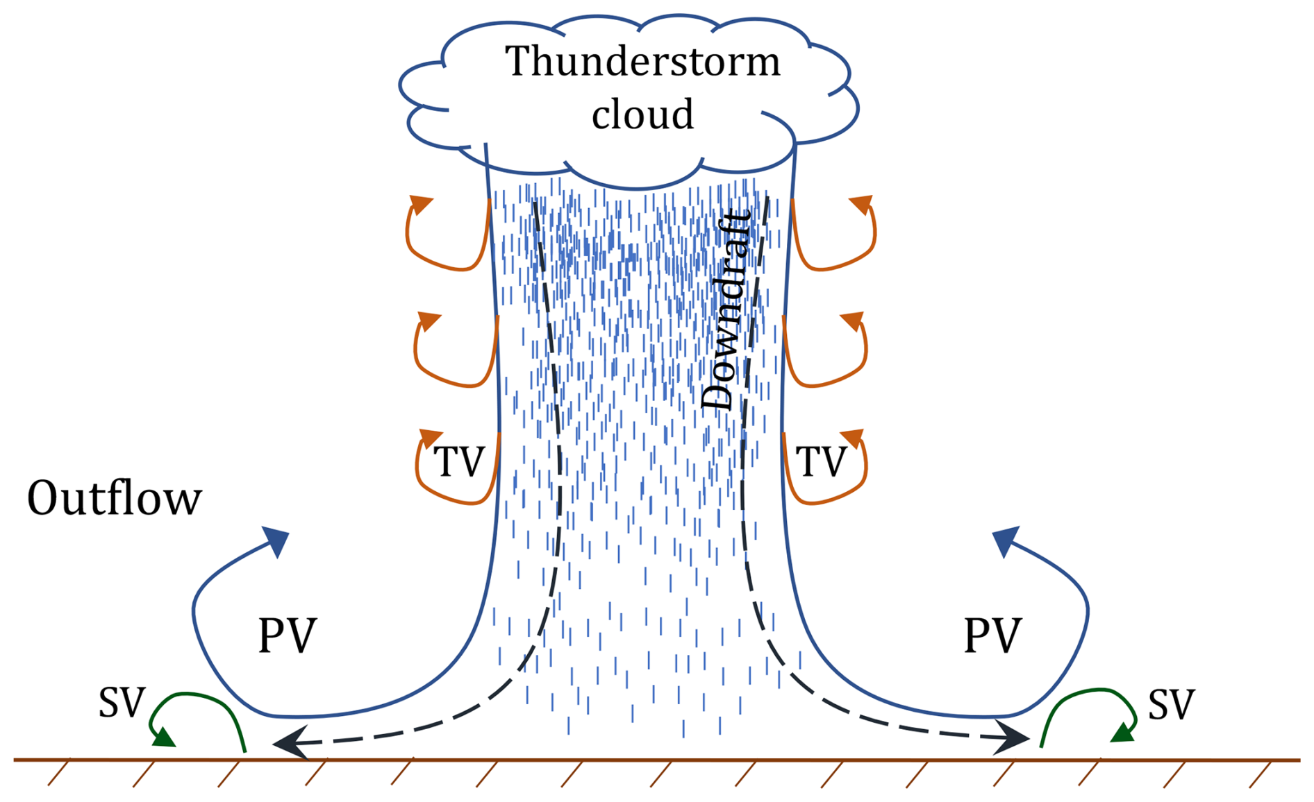
Figure 1 Schematic representation of a thunderstorm downburst, illustrating the primary, secondary, and trailing vortical structures.

Thunderstorm winds, particularly downbursts, are transient and develop within a short timeframe (a few minutes or tens of minutes) over a limited spatial extent (a few to a few tens of kilometers) (Fujita, 1981). This makes their full characterization challenging. Traditional measurement tools like anemometers, as well as advanced remote-sensing instruments such as Light Detection and Ranging (LiDAR) profilers, scanners, and radars, can only provide partial snapshots of these events. These limitations arise due to variations in the relative position between the storm and the instrument, as well as differences in downburst characteristics. Furthermore, we miss essential physical contributions to its genesis and overall structure. As a result, we often lack a comprehensive understanding of the physical processes that generate and shape these winds, which is essential for developing accurate flow field models for structural design and meteorological standards.

Addressing the complexity of downbursts requires either controlled physical simulations in specialized laboratories and/or numerical modeling. While advancements in computational power have significantly improved the ability to replicate the three-dimensional and transient nature of these phenomena (Žužul et al., 2024), computational fluid dynamics (CFD) simulations still struggle resolving turbulence, instabilities, and thermal effects without prohibitive computational cost. Experimental methods are well-established but only a few laboratories worldwide are capable of reproducing downbursts at the relevant Reynolds numbers for civil and wind engineering applications. Currently, no wind simulator can fully reproduce the thermomechanical mechanisms responsible for the formation and evolution of downburst winds at large geometric and kinematic scales.

Two experimental methods are typically used to simulate downburst-like winds: (i) the gravity current (GC) method (Simpson, 1969; Charba, 1974; Lundgren et al., 1992; Yao and Lundgren, 1996), where the downburst is driven by the buoyant force arising from the density difference between the heavier downdraft and the lighter surrounding fluid; and (ii) the impinging jet (IJ) method (Brady and Ludwig, 1963; Canepa et al., 2022a; Didden and Ho, 1985; Gutmark et al., 1978; McConville et al., 2009; Romanic et al., 2019; Sengupta and Sarkar, 2008; Xu and Hangan, 2008), where the downburst is mechanically initiated by forcing air into the environment using air fans, generating a jet of similar temperature and density. The GC method is more accurate in replicating the real-world conditions of a downburst, including the horizontal pressure gradients caused by air density and temperature differences. However, these experiments are often performed with fluids other than air to match non-dimensional parameters, such as the Richardson number, resulting in low velocities and small-scale experiments that are less relevant for practical engineering applications. In contrast, the IJ method does not fully replicate the thermodynamic processes of downbursts, but it can reproduce the spatial and temporal evolution of the near-ground flow field with higher velocities, making it more suitable for structural and environmental investigations. As a result, the IJ method has been more widely adopted in recent research also in the view of implementation into design recommendations.

However, this raises an important question: Does the IJ method accurately simulate downburst flow at the ground, or do buoyancy effects significantly influence the downburst's geometric and dynamic evolution? In nature, the cold and dense air from a thunderstorm cloud falls due to thermal contrast with the surrounding atmosphere (as seen in GC experiments) creating a downdraft. Despite lateral entrainment of warmer air into the jet, weather stations typically record temperature drops of up to about 10 °C during the passage of a downburst outflow (Choi, 2004; Choi and Hidayat, 2002; Huang et al., 2019). The largest temperature decrease reported to date – 12.9 °C – was recorded in Romania (Calotescu et al., 2025), to the best authors' knowledge. The greater the amount of buoyant energy available in the troposphere in the form of warm and humid air – typically quantified by the Convective Available Potential Energy (CAPE) parameter – the higher the potential for intense updrafts and formation of deep convective clouds that may produce violent thunderstorms. The Downdraft Convective Available Potential Energy (DCAPE) considers the thermodynamic characteristics of the mid and lower parts of the atmosphere, often below the storm cloud base, to assess the energy that an air parcel might gain as it descends toward the surface. High DCAPE values indicate the potential for stronger downdrafts approaching the ground, resulting in a more vigorous near-ground outflow. This raises further questions about how gravity currents and the temperature difference between the downdraft and surrounding air may affect the geometric characteristics and size of vortex structures in the downburst system. When applied at larger geometric scales and using air with varying thermal properties, the GC technique could ultimately provide answers to these questions.

To address these aspects, the CLIMATHUNDERR project (CLIMAtic Investigation of THUNDERstorm Winds) was initiated at the Jules Verne Climatic Wind Tunnel (JVCWT) – Thermal Unit SC2 at the Centre Scientifique et Technique du Bâtiment (CSTB) in Nantes, France. Funded by the European Union's European Research Infrastructures for European Synergies (ERIES) project, this project builds on the experimental campaigns (Canepa et al., 2022a, b, c, 2023, 2024a), conducted in recent years at the WindEEE Dome at Western University in Canada, under the ERC project THUNDERR – Detection, simulation, modelling and loading of thunderstorm outflows to design wind-safer and cost-efficient structures (Solari et al., 2020). The CLIMATHUNDERR acronym is intentionally inspired by the previous THUNDERR project, reflecting continuity while expanding its focus to include the thermal effects on thunderstorm winds.

In this project, varying thermal contrasts between the jet and the ambient air were tested to investigate the buoyancy effects on the velocity, dynamics, and geometric features of the downburst at the ground level. Large-scale Particle Image Velocimetry (LS-PIV) was employed to capture variations in the flow field, and thermocouples were used to monitor temperature profiles. To the best authors' knowledge, this experimental campaign is unique, as the GC method has not previously been applied at such large geometric scales and using only air as fluid.

Additionally, the reproduced downburst flows were tested over a 1:2000 scale model of the Polcevera Valley in the municipality of Genoa, Italy, to assess the influence of local orography on the flow dynamics and vortical structures development. Meteorological observations and high-frequency anemometric measurements (Solari et al., 2012; Repetto et al., 2018; Burlando et al., 2018, 2020; Canepa et al., 2020, 2024b; De Gaetano et al., 2014) provide compelling evidence that this region is highly susceptible to the formation of thunderstorms. This vulnerability stems from the proximity of the Mediterranean Sea, serving as a source of warm and humid air essential for the initiation of air updrafts (Giorgi, 2006; Púčik et al., 2017; Lolis, 2024). Additionally, the Ligurian Apennines mountain range plays a crucial role by ushering in cold air. This combination creates intense convective conditions that often lead to downbursts approaching Genoa from the south-southwest. This setup was replicated in the JVCWT experiments.

All data from the project are publicly available via the Zenodo repository and can be re-used under Creative Commons license CC0 for metadata and CC-BY for data (Canepa et al., 2025a).

The paper is organized as follows: Sect. 2 provides an overview of the CLIMATHUNDERR project, followed by a detailed description of the experimental setup, specimens, and instrumentation specifications in Sect. 3. Section 4 offers guidance on using the published dataset, while Sect. 5 provides a preview of its content. Section 6 closes the paper with conclusions and perspectives.

2 CLIMATHUNDERR project

The CLIMATHUNDERR project – CLIMAtic Investigation of THUNDERstorm Winds – was selected by the ERIES' evaluation panel to conduct experimental research at the JVCWT facility in the CSTB laboratory, Nantes, France. The project is funded by the European Commission's Horizon 2021 program. The User Group (UG) consists of researchers from leading universities in Italy and Canada, bringing together a multidisciplinary expertise on thunderstorm winds.

UG members come from a wide range of disciplines, including atmospheric physics, meteorology, experimental and numerical fluid dynamics, as well as civil and mechanical engineering. Collectively, they bring extensive expertise in studying thunderstorm winds from multiple perspectives. This includes full-scale field campaigns using anemometric and LiDAR profiler instruments (Burlando et al., 2017, 2018, 2020; Canepa et al., 2020, 2024b; Romanic et al., 2020c; Romanic, 2021; Zhang et al., 2018), experimental studies utilizing anemometric and PIV measurements (Canepa et al., 2022a, b, c, 2023, 2024a; Hangan et al., 2019; Junayed et al., 2019; Romanic et al., 2019, 2020a, c; Romanic and Hangan, 2020; Xu and Hangan, 2008) at the WindEEE Dome, one of the largest wind simulators capable of reproducing large-scale, non-stationary extreme wind events (Hangan et al., 2017). Additionally, the CFD modeling technique has been employed in various studies (Kim and Hangan, 2007; Žužul et al., 2023, 2024). These combined experimental and numerical approaches are being synthesized to develop a state-of-the-art analytical model for thunderstorm winds (Xhelaj et al., 2020; Xhelaj and Burlando, 2022, 2024). The model will be further enhanced by incorporating results from the current experiments to account for the thermal effects on downburst wind evolution. This enhancement will be achieved by developing a full 3D analytical model whose formulation, derived through dimensional analysis using the Buckingham Pi theorem, reduces parameter complexity and ensures consistent scaling. The model will be capable of accurately reproducing temperature-dependent vertical profiles of radial velocity and the associated vortex dynamics. These features will be informed by reduced-order models obtained through Proper Orthogonal Decomposition (POD), thereby providing a more physically representative description of natural downbursts.

The implementation of the CLIMATHUNDERR experimental campaign was made possible through the crucial contributions of the technical staff at CSTB. The design of the experimental setup involved close collaboration between the UG and the CSTB technical staff, resulting in a highly complex, innovative, and unique experimental apparatus, specifically crafted to meet the project's objectives.

3 Experimental setup

The experiments were conducted in June 2024 at the JVCWT – Thermal Unit SC2, located at CSTB in Nantes, France. This section provides a detailed description of the thermal-wind simulator, the specimen and measuring techniques involved, as well as the overall test plan and operational setup.

3.1 Facility

The JVCWT, built in the 1990s, consists of two concentric wind tunnels: the outer ring is called “dynamic circuit” and the inner one is called “thermal circuit”. These wind tunnels allow comprehensive and full-scale aero-climatic simulations. The thermal circuit, where all data in this study was collected, can replicate a wide range of real-world climatic conditions, including rain, snow, frost, and solar radiation.

Figure 2 shows a schematic of the thermal circuit wind tunnel. The test section measures 10 m in width (W), 7 m in height (H), and 25 m in length (L). At the downstream end, a sudden contraction leads into a 180° turn. Upstream of the fan, the cross-section transitions from rectangular to circular, with a diameter of 6.2 m to guide the airflow into the fan.

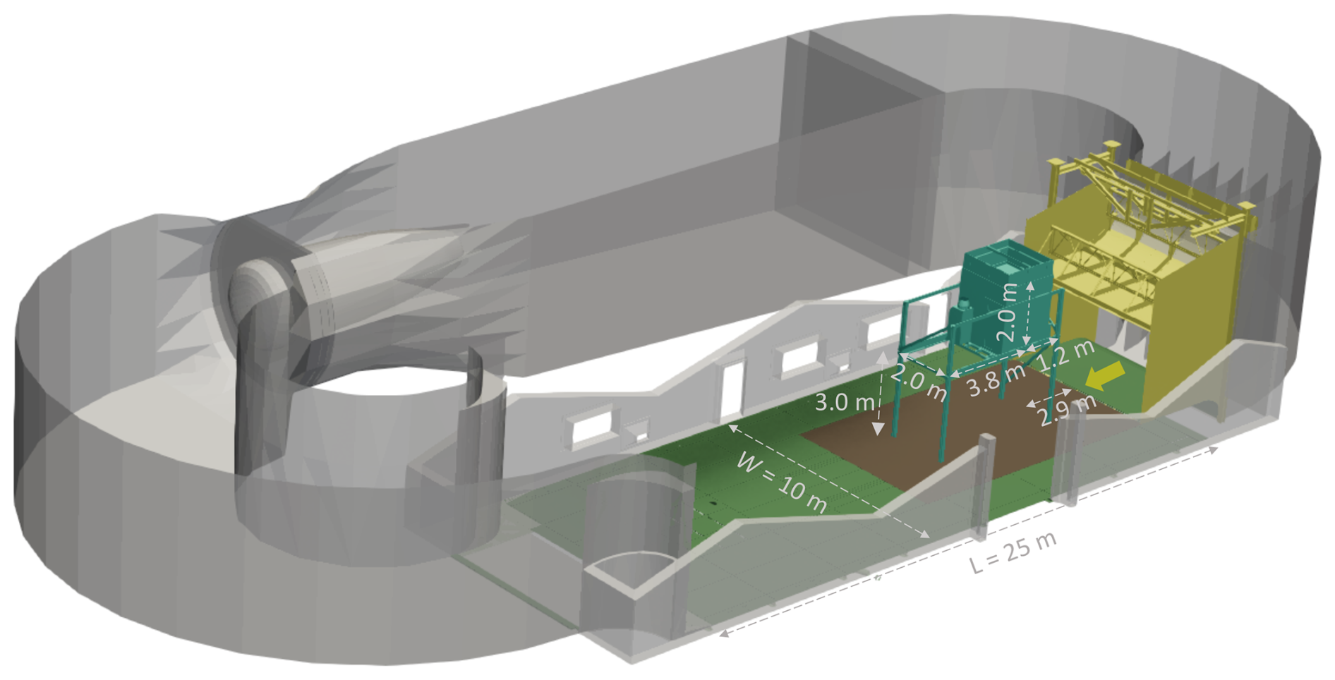
Figure 2 Schematic of the thermal circuit wind tunnel with relevant dimensions of the testing chamber. Yellow arrow shows the upstream orientation.

The variable-speed axial fan, with a power of 1100 kW, can generate steady wind speeds between 1 and 40 m s⁻¹. A heat exchanger is positioned downstream of the fan blades, while the adjustable nozzle creates a contraction from the cross-section after the second 180° turn (6×9 m²) to an area ranging from 6×5 m² to 6×3 m². This contraction is controlled by lowering the ceiling height over a distance of 3 to 5 m, allowing the wind flow to discharge into the larger test section through the nozzle exit.

This climatic wind tunnel differs from a typical boundary layer wind tunnel in several key aspects. Notably, the shorter fetch, presence of flow disturbances and separations, and a longitudinal pressure gradient all contribute to challenges in generating a stable atmospheric boundary layer (ABL) within the testing chamber.

3.2 Specimen and geometry

The primary technical challenge of the experimental setup involved creating a downdraft-like jet from scratch. This required a mechanism capable of producing a vertical, top-down air jet within the testing chamber. In recent years, various wind simulators have been developed to generate vertical air flows, either by blowing or sucking air, to simulate top-down or bottom-up jets that closely mimic natural downbursts or tornadoes, respectively (Haan et al., 2008; McConville et al., 2009; Hangan et al., 2017; Li et al., 2024). For this setup, an upper plenum with dimensions of $\mathrm{2}\times \mathrm{2}\times \mathrm{2}$ m³ was constructed, hereafter referred to as the impinging-jet plenum (IJP). The IJP's walls were made of 15 mm thick plywood lined with insulation material to minimize thermal losses and prevent air stratification, in order to ensure a stable temperature differential (ΔT) between the plenum and the testing chamber. Figure 3a and b show the IJP installed in the testing chamber during the tests. A 7.3 kW Coolmobile 25 air conditioning unit, manufactured by Thermobile Industries B.V., was installed outside one of the IJP's side walls and connected via three tubes to cool the internal air to a minimum temperature below 10 °C (Fig. 3a and b). Beside blowing cold air into the IJP, the Coolmobile 25 also sucked air from it, forming a closed thermal circuit between the IJP and the Coolmobile unit.

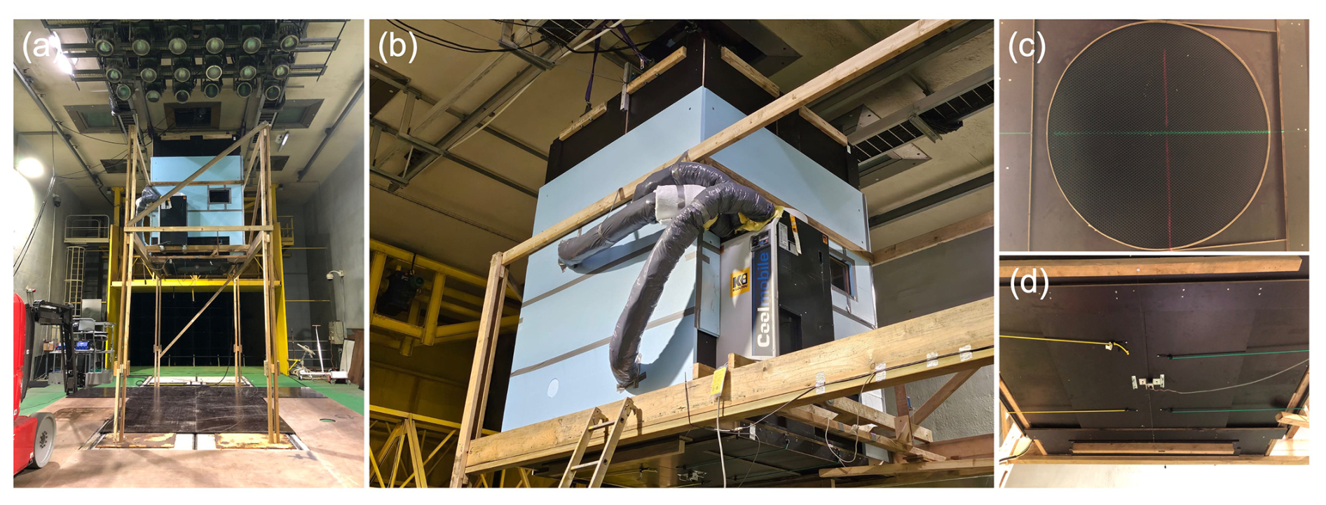
Figure 3 (a) IJP mounted on a wooden frame in the testing chamber; (b) zoom-in on the IJP and air conditioning unit; (c) open nozzle with honeycomb; (d) closed nozzle with louvers.

Three additional windows (transparent plates) were included in the IJP design: two on the downstream side for visual inspection of the IJP's interior during experiments; and another, with dimensions 0.8×0.18 m², at the bottom of the upstream wall to feed PIV seeding particles into the IJP – in a closed volume – before starting an experiment. It was ensured that no leakage was present.

The ambient air in the testing chamber, without active control from heat exchangers, was around 25 °C. The frontier between IJP and testing chamber was a circular opening (nozzle) with a diameter D=1 m, located at the center of the IJP's bottom panel. The nozzle was equipped with a honeycomb structure (Fig. 3c) – a 100 mm thick hexagonal mesh with a grid diameter of 12 mm and an aluminium sheet thickness of 0.07 mm – designed to reduce the turbulence level and increase the homogeneity in the outgoing jet. The nozzle was positioned H=3 m above the chamber floor, resulting in $H/D>\mathrm{1}$. For this configuration the confinement effects are negligible, allowing the primary vortex (PV) leading the downburst outflow to fully develop (Xu and Hangan, 2008; Junayed et al., 2019). A mechanism to control the nozzle's opening was developed to simulate the transient nature of real downbursts and to synchronize all the measurements from the start of the experiment. This was achieved with two rectangular wooden louvers held together by a central magnet (Fig. 3d). At the desired time, the magnetic current was switched off, causing four elastic tensioners – two on each side – to pull the louvers apart instantly (time of complete opening about 0.3 s). Additionally, a piston with dimensions $\mathrm{2}\times \mathrm{2}\times \mathrm{0.6}$ m³ was located at the top of the IJP (visible above the light blue walls of the IJP in Fig. 3a and b) and was suspended from the testing chamber ceiling by means of a winch. A distance sensor measures piston speed and triggers the piston to stop before reaching the bottom of the IJP.

The IJP was mounted in the testing chamber on a robust wooden frame with planar dimensions of 5 (L) × 2 (W) m² (Fig. 3a).

The frame was placed 2.9 m from the outlet of the wind tunnel's nozzle (Fig. 2). The center of the IJP nozzle was 1.2 m from the upstream edge of the wooden frame, providing a 3.8 m horizontal fetch for LS-PIV measurements (Fig. 2). This horizontal stretch was covered by a 0.015 m thin wooden panel to level the ground and reproduce a smooth floor with roughness very close to zero (Figs. 2 and 3a).

The second part of the experimental campaign focused on assessing the downburst-like flows on a 1:2000 scale orography model of the Polcevera Valley, located in the municipality of Genoa, Italy (Fig. 4). The full-scale representation covered an area of 7 km (L) × 4 km (W), spanning from the Genoa-Voltri commercial port in the Ligurian Sea to the inland hilly regions that mark Genoa's northern boundaries. Key landmarks, such as the Erzelli hill (site of Italy's largest science and technology park) and the San Giorgio Bridge (rebuilt after the tragic collapse of the Morandi Bridge), were included in the model. The scaled model has horizontal dimensions of 3.5 m (L) × 2 m (W) while the highest orographic point was 0.297 m height (H). The model was mounted on a rectangular panel with a thickness of 0.015 m, while the corresponding wooden panel on the testing chamber floor was removed for this section so that the model's bottom surface (representing sea level) was flush with the chamber floor. The model was manufactured using 3 and 5 axis digital milling, with 15 and 16 mm hemispherical cutters, on lightweight (23 kg m⁻³) expanded polystyrene (EPS). The surface was painted matte black to minimize reflections from the laser used for PIV measurements (see Sect. 3.4.1). The model was installed in the chamber so that its transversal section was centered at the geometric location of the jet touchdown. The longitudinal position varied between two configurations, as will be discussed later.

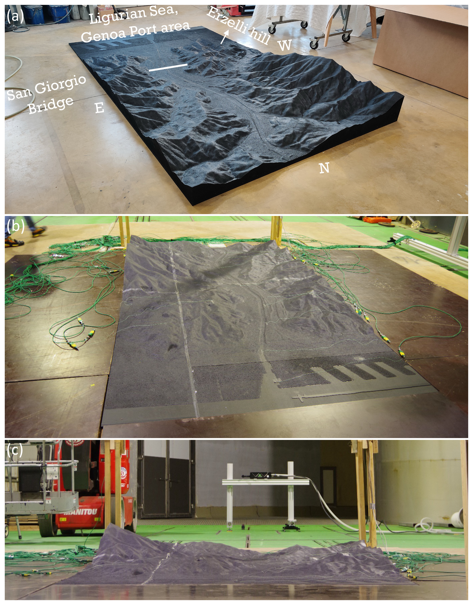
Figure 4 The 1:2000 orography model of the Polcevera Valley in the Municipality of Genoa, Italy, with key locations and approximate cardinal points shown (a) and close-up views from the geographical south (b, c).

3.3 Formation of buoyancy-driven impinging jets

The formation of the gravity-current impinging jet in our experimental setup was achieved through a combination of two techniques: a mechanically-driven IJ and a GC created by a temperature differential (ΔT). The mechanical aspect involved generating overpressure into the IJP air using a piston that moved downward over a 2-m vertical distance (IJP's height) through a winch, while the buoyancy component arose from the ΔT between the cooled IJP air and the warmer chamber air. Ideally, a purely buoyancy-driven jet would best replicate natural downburst events. However, the mechanical contribution of the piston was necessary to regulate the jet speed at the nozzle exit and therefore control the initial test conditions and ensure repeatability of the start of the experiments. Preliminary theoretical calculations, based on the Navier-Stokes equation along the vertical axis (z) and neglecting viscous effects, allowed to estimate the expected buoyant jet velocities w_B at the near-impingement level:

$$\begin{array}{}\text{(1)}& {\displaystyle \frac{\mathrm{d}{w}_{\mathrm{B}}}{\mathrm{d}t}}=-{\displaystyle \frac{\mathrm{1}}{\mathit{\rho }}}{\displaystyle \frac{\mathit{\delta }p}{\mathit{\delta }z}}-g\end{array}$$

where w_B is the expected vertical buoyant jet velocity, ρ=1.23 kg m⁻³ is the air's reference density value, t is the time, $\mathit{\delta }p/\mathit{\delta }z$ is the vertical pressure gradient with p being the total pressure and z denoting the upward-pointing vertical coordinate, and g=9.81 m s⁻² is the gravitational acceleration. Particularly, ρ can be assumed as constant as temperature and pressure variations within the chamber are not significant enough to cause substantial density changes beyond the primary temperature differential (ΔT) that drives the buoyant jet.

By treating the air as an ideal gas and introducing hydrostatic approximation, the buoyancy term (B), which drives the downward acceleration of the jet, can be expressed as:

$$\begin{array}{}\text{(2)}& B={\displaystyle \frac{\mathrm{d}{w}_{\mathrm{B}}}{\mathrm{d}t}}={\displaystyle \frac{\left|T_{\mathrm{IJP}}-T_{\mathrm{env}}\right|}{T_{\mathrm{env}}}}g={\displaystyle \frac{\mathrm{\Delta }T}{T_{\mathrm{env}}}}g\end{array}$$

where T_IJP and T_env are respectively the air temperature inside the IJP and in the chamber before the release of the jet. Through integration and application of the Galilean transformation $\mathrm{d}t=\mathrm{d}s/w$ (being s the spatial coordinate), the velocity of the buoyancy-driven jet at the near-ground, w_B, becomes:

$$\begin{array}{}\text{(3)}& \begin{array}{rl}& \underset{\mathrm{0}}{\overset{w}{\int }}{w}_{\mathrm{B}}\mathrm{d}w={\displaystyle \frac{\mathrm{\Delta }T}{T_{\mathrm{env}}}}g\underset{\mathrm{0}}{\overset{H}{\int }}\mathrm{d}s\\ & w_{\mathrm{B}}=\sqrt{\mathrm{2}HB}\end{array}\end{array}$$

where H=3 m is the nozzle-to-ground height. Using the maximum designed ΔT for the experiments of 25 °C (for T_env=35 °C), a theoretical buoyancy-driven jet velocity at the ground of w_B=2.18 m s⁻¹ was calculated. In reality, this velocity would be lower due to flow dispersion and entrainment of the warmer ambient air, which reduces the jet's vertical speed.

To better simulate the atmospheric thermal conditions during downbursts, our goal was to replicate the Richardson number (Ri) of full-scale events as closely as possible. Ri is a dimensionless quantity that expresses the ratio of buoyancy to inertial forces in the flow or, in the case of thermal convection, the relative importance of natural vs. forced convection:

$$\begin{array}{}\text{(4)}& Ri={\displaystyle \frac{g\mathit{\beta }\mathrm{\Delta }TD}{w^{\mathrm{2}}}}\end{array}$$

where β=0.00367 $\mathrm{1}/K$ is the air's thermal expansion coefficient (assumed constant at 25 °C), and D is the jet diameter. Here, w arises from the combination of buoyancy-driven (w_B) and mechanically-driven (w_IJ) velocities, as determining the exact contribution of each is not feasible.

For a full-scale jet with diameter D_FS=1000 m, cloud-exit speed of 10 m s⁻¹, and a temperature difference ΔT_FS=10 °C, we obtain an approximate Richardson number Ri≈3.6, which decreases to about 0.9 with a jet speed of 20 m s⁻¹. These values reflect a transition from buoyancy-dominated to shear-dominated flow regimes. However, it is important to note that full-scale downbursts exhibit a wide range of Ri depending on specific atmospheric conditions driving different downburst events. The full-scale Ri values suggest that our experiments would require very low jet velocities to replicate the full-scale conditions. However, achieving such low velocities in the wind tunnel would result in an unstable jet. Therefore, we slightly increased the jet velocity to maintain stability, even though this meant deviating from the ideal Ri value. Despite Ri values in our geometrically-scaled experiments are generally lower than those observed in natural downbursts, the experimental campaign was designed to systematically vary this parameter. The Ri for each run, calculated theoretically using the measured ΔT and total jet velocity $w=w_{\mathrm{IJ}}+w_{\mathrm{B}}$, is explicitly provided in Table 2. This allows users to directly investigate the impact of Ri variability on flow dynamics, and study the trends and mechanisms of buoyancy-inertia interaction under controlled conditions in downburst-like flows.

In our experiments, ΔT values ranged approximately from 0 °C (as a baseline) to 25 °C. To generate a temperature differential, an air conditioning unit was used to cool the air inside the IJP to a minimum of approximately 6–10 °C. Heat exchangers located downstream of the wind tunnel fan maintained the ambient temperature around 25 °C or warmed it. To minimize vertical temperature stratification in the testing section, the fan was initially run for approximately 5 min at approximately 3 m s⁻¹ to circulate warm air into the chamber, then shut off 1 min before each experimental run, along with the air conditioning system.

Two thermocouples were placed inside the IJP – near the bottom and top surface – to monitor the temperature distribution, while two more thermocouples were positioned along the jet's vertical centerline, at ground level and 2.90 m a.g.l. (above ground level) (0.10 m below the nozzle outlet section) (Fig. 7). Despite the efforts, achieving steady ΔT conditions was challenging due to: (i) thermal diffusion; (ii) the incomplete insulation of the IJP; (iii) efficiency variation of the air conditioning system, which systematically switched to a “defrosting” mode lasting approximately 4 min after each experimental run.

1000 ms after the nozzle opened, the piston was released downward at two different velocities, w_p=0.15 m s⁻¹ or 0.25 m s⁻¹, covering a vertical distance of 2 m. This produced a purely mechanically-driven impinging jet with estimated velocities w_IJ of about 0.8 and 1.3 m s⁻¹ (Table 2), respectively, based on the flow rate conservation:

$$\begin{array}{}\text{(5)}& w_{\mathrm{p}}{A}_{\mathrm{IJP}}=w_{\mathrm{IJ}}{A}_{\mathrm{op}}\end{array}$$

where A_IJP and A_op are the cross-section areas of the IJP and nozzle, respectively. With $H/D=\mathrm{3}$, w_IJ remains nearly constant along the jet and can be assumed equal to the exit velocity (Pope, 2000).

The mechanically-driven IJ, combined with the temperature differential applied between the IJP and the chamber air, produces a thermal impinging jet, conceptually similar to naturally occurring downbursts. The predicted total jet velocity (prior to PIV measurements) was conceptualized as a combination of the two independently determined contributions: $w=w_{\mathrm{IJ}}+w_{\mathrm{GC}}$ (Eq. 4), where w_IJ represents the mechanically-driven impinging jet velocity, and w_GC=w_B represents the buoyancy-driven gravity current, as outlined earlier. The PIV system then directly measures the actual total vertical velocity, allowing for a comparison with its predicted value. Table 2 also reports the Richardson number based on the total jet velocity w_exp obtained from the PIV measurements, denoted as Ri_exp. w_exp is evaluated only for the experimental cases without the model installed due to the different positioning of the PIV field of view (FOV) not capturing the jet phase (see Sect. 3.4.1). Specifically, w_exp is computed as the average vertical velocity evaluated: (i) spatially, over the vertical and horizontal coordinate ranges 750–1250 and 0–250 mm, respectively; and (ii) temporally, for the spatial region defined in (i), over the sub-interval during which w_exp can be regarded as quasi-constant. This time interval is identified as the longest continuous segment for which the temporal variation satisfies dw_smooth<5 %w_smooth, where w_smooth is the moving average of the spatially averaged velocity computed using a 0.5 s window.

The selection of these spatial and temporal ranges is motivated by two main considerations: (i) allowing buoyancy effects to develop along the jet, while simultaneously avoiding the influence of the near-ground pressure bubble that forms as the jet approaches the impingement region, where the flow transitions from vertical to horizontal and the jet velocity is reduced; and (ii) ensuring that w_exp is as stationary as possible, so that it can be considered representative of the characteristic jet velocity.

The higher values of Ri_exp compared with the theoretical estimates are attributable to the lower w_exp observed in the experiments, resulting from flow dispersion and entrainment of the warmer ambient chamber air, which reduce the jet speed, as discussed above.

The Reynolds number, defined as $Re=w_{\mathrm{jet}}D/\mathit{\nu }$ (where ν=1.48 m² s⁻¹ is the kinematic viscosity of air, assumed constant based on the reference air density specified above) varies between 5.07×10⁴ and 9.12×10⁴ when computed using only the mechanical velocity (w_jet=w_IJ), and between 6.97×10⁴ and 2.19×10⁵ when the buoyancy-induced velocity component is also included (w_jet=w).

The duration of the reproduced downburst release from the IJP, resembling the situation of downdraft discharging from a thunderstorm cloud in nature, corresponded to the time it took for the piston to cover the 2 m vertical distance in the IJP, approximately 13 s at 0.15 m s⁻¹ and 8 s at 0.25 m s⁻¹. Each experimental run lasted 30 s from the nozzle louvers' opening (t=0). All experimental signals were synchronized based on this time reference. A dedicated control software was developed in LabVIEW to automate the sequence: (i) at t=0, a TTL (Transistor-Transistor Logic) signal triggered the PIV system, initiated the acquisition of all other measurements, and activated the opening of the nozzle louvers; (ii) at t=1000 ms, the power supply to the winch was enabled, allowing the piston to descend along its 2 m stroke.

3.4 Measurement instrumentation

3.4.1 Large-scale Particle Image Velocimetry (LS-PIV)

The Large-Scale Particle Image Velocimetry (LS-PIV) technique was used, as it allows capturing instantaneous velocity fields over large areas. Unlike point velocity measurement instruments, such as multi-hole pressure probes or hot wires, LS-PIV enables all four capabilities simultaneously: accurately measuring low velocities, characterizing flows with strong recirculation, remaining unaffected by sudden temperature fluctuations, and achieving high spatial resolution.

The fluid was seeded with Helium-Filled Soap Bubbles (HFSB), averaging 300 µm in diameter. Helium bubbles – a recent advancement in PIV (e.g., Bosbach et al., 2009; Scarano et al., 2015) – are optimal due to their low weight (approximately 1000 times lighter than standard oil aerosol particles), a relaxation time of 11 µs, long bubble lifetimes of several minutes, and high seeding concentrations (up to 1300 bubbles per cubic centimeter at the nozzle exit). A microprocessor-controlled device automatically managed the flow rates of air, helium, and soap during the experiments. The seeding particles were injected into the IJP during the cold air fill through 40 nozzles connected to a rectangular opening in the upstream lateral panel of the IJP.

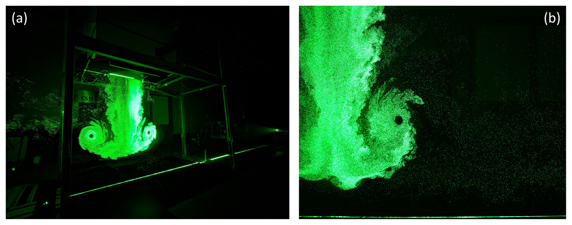
Figure 5 Evolving downburst and PV travelling downward: (a) photograph from an external camera and (b) raw image from LS-PIV acquisition with helium bubbles as illuminated by the laser beam.

A dual pulsed laser (Nd:YAG EverGreen manufactured by Quantel), with a wavelength of 532 nm, was employed to illuminate the particles (Fig. 5). Each double pulse operated at a maximum repetition rate of 15 Hz, producing an output energy of 200 mJ per pulse. Positioned about 17 m downstream from the main chamber nozzle, the laser illuminated a thin vertical layer precisely aligned with the jet centerline. A combination of spherical and cylindrical lenses generated a uniform 20 mm laser sheet from the laser beam. A synchronizer (PTU X) controlled the timing between laser pulses and camera exposure time.

Two cameras provided by LaVision were used (not simultaneously) for image acquisition. The first was the Imager Pro X 4M, equipped with a CCD sensor, with resolution 4 MP, 14 bits digital output, and a maximum frame rate of 15 fps in single frame. Due to failure at experiment #15 (see Sect. 3.5), it was replaced with an Imager SX6M, with a CMOS sensor, resolution 6 MP, 12 bits digital output, and a maximum frame rate of 25 fps in single frame. The pixel-to-meter conversion was performed using a calibration target. The origin of the camera's vertical FOV (r₀, $z_{\mathrm{0}})=(\mathrm{0},\mathrm{0})$ corresponded to the jet vertical centerline and floor level, respectively. The FOV was aligned with the jet diameter in the testing chamber streamwise direction. The first camera's FOV spanned approximately 2.5×2.5 m², covering longitudinal (r) and vertical (z) coordinates of approximately 26 to 2488 mm and −29 to 2451 mm, respectively, with a resolution of 18.65 mm. The second camera's FOV extended to 3.2×2.5 m², with limits of approximately −396 to 2822 mm in r and −38 to 2502 mm in z, achieving a resolution of 15.78 mm. Negative z values are due to the FOV including a small portion of the ground floor. Speed measurements are displayed as valid and different from 0 only for z>0. From experiments #40 to #57 (tests with the orography model), the FOV shifted as detailed below. The large FOV enabled coverage of the horizontal flow field from $r/D=\mathrm{0}$ to $r/D=\mathrm{2.5}$ and 3.2, respectively, and a vertical extension from $z/D=\mathrm{0}$ to $z/D=\mathrm{2.5}$ (0.50 m below the nozzle outlet). In this context, r represents the radial (longitudinal) distance from the jet vertical centerline, z denotes the height above the ground floor, and D=1.0 m is the jet diameter. This window captures all critical regions of the reproduced downburst wind (Canepa et al., 2022a, b; Junayed et al., 2019): the downdraft stage, reaching $r/D=\mathrm{0.5}$ (the edge of the IJ diameter), and extending beyond due to the jet widening at the nozzle exit; the downburst ramp-up and peak intensity produced by the propagation of the PV on the horizontal and possible interaction with the secondary vortex (SV); the downburst slow-down and dissipation due to smaller and weaker trailing vortices (TV) following PV and to the system energy decay (i.e., nozzle closing in the experiments). Literature suggests that $r/D=\mathrm{1.0}$ corresponds to the approximate position of maximum wind speed in the outflow (Canepa et al., 2022b; Simpson, 1969; McConville et al., 2009; Chay and Letchford, 2002). A LS-PIV window height of 2.5 m above the floor also allows complete detection of the PV structure during its radial and temporal evolution (Junayed et al., 2019). The assumption of radial symmetry of the impinging jet and developing outflow at the ground allows for extending the results to any radial direction from the jet touchdown center. To accommodate the large FOV with high spatial resolution, PIV pairs of images were recorded at 7 and 12 Hz, respectively for the two cameras in double frame mode.

A commercial software (DAVIS 10) was used to calculate velocity and other parameters (see Sect. 4) from the raw images. The software uses the standard Fast Fourier Transform correlation to compute particle displacement, with an interrogation window size of 32 pixels by 32 pixels with 50 % overlap for processing.

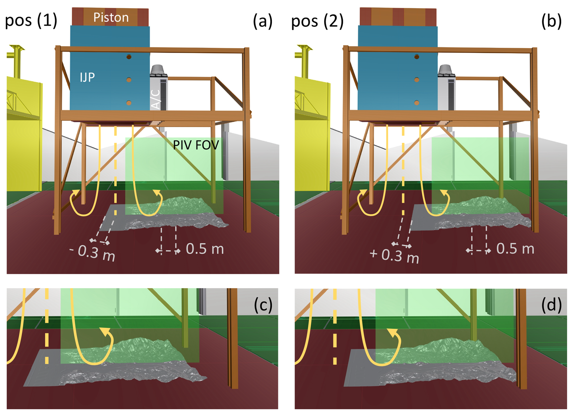
Figure 6 Schematics of experimental specimen and orography model configurations (not-to-scale). (c) and (d) are zoom-ins on configurations pos (1) (a) and pos (2) (b), respectively. Yellow arrows and vertical dashed line indicate the PV circulation and the jet axis, respectively. The green rectangle shows the PIV FOV.

The scaled orography model and PIV camera were installed at two different positions relative to the jet centerline to examine the downdraft touchdown in two scenarios: (i) on open sea outside the port area and (ii) on the port area itself. According to the downdraft position, the downburst outflow stage varies significantly over the orography of Genoa in terms of dynamics, intensity, and geometry. Specifically, the southern edge (port-area side at the dam) of the model was positioned at ±0.3 m from the geometric center of the IJ touchdown, corresponding to a real downburst landing approximately 600 m onshore and offshore relative to the port dam, designated as positions pos (1) and pos (2) in the experimental setup schematics (Fig. 6). The camera FOV (approx. 3.2×2.5 m²) was adjusted to focus on the same portion of the model in both situations: the center of the camera's longitudinal coordinate was positioned at +0.5 m relative to the geometric center of the model, downwind of the IJ outflow. This setup allowed both FOVs to record the downburst outflow evolution within the reduced-scale valley and potential flow channeling effects. For position (1), the camera's FOV spanned approximately 304 to 3522 mm in r and −38 to 2502 mm in z. For position (2), the FOV shifted 600 mm downstream, with longitudinal coordinate limits of 904 and 4122 mm, while the z-limits remained unchanged. This corresponds to a portion of the downburst outflow being captured within the range of approximately $r/D=\mathrm{0.3}$ to 3.5 (model in position 1), and $r/D=\mathrm{0.9}$ to 4.1 (model in position 2).

3.4.2 Temperature measurements

In the experiments conducted without the model, 20 fast-response thermocouples (about 0.5 s reaction time) (designated as “Tf” and indicated by orange numbers in Fig. 7) were utilized to capture the transient temperature profiles associated with the onset and passage of the downburst outflow. The thermocouples' model was 5SRTC-TT-KI-40-1M, manufactured by Omega Engineering Ltd., featuring a K-type sensor with a diameter of 0.076 mm. 18 thermocouples were distributed across four radial locations $r/D=\mathrm{1.0}$, 1.5, 2.0, and 2.5. They were arranged vertically at z=0, 0.10, 0.20, 0.40, and 0.60 m (corresponding to $z/D=\mathrm{0}$, 0.10, 0.20, 0.40, 0.60), except for $r/D=\mathrm{2.5}$, where thermocouples were placed only at z=0, 0.20, and 0.60 m. The thermocouples were mounted along thin vertical wires bolted to the wooden floor panel and secured to a horizontal wood beam overhead. The minimal thickness of the wires and thermocouples ensured that they had no impact on the flow field. To avoid potential disturbances to the PIV laser and FOV, the thermocouples were installed along a downburst radial direction shifted 18.5° anticlockwise (opposite side of PIV camera position, see Fig. 9a) from the LS-PIV vertical plane aligned with the chamber's longitudinal direction. The remaining two thermocouples were positioned along the jet's vertical centerline at $z/D=\mathrm{0}$ and 2.90, with the latter suspended horizontally below the nozzle. Additionally, four slower (reacting time approximately 1 s) “standard” thermocouples (denoted as “Ts” and indicated by blue numbers in Fig. 7), K-type, with insulated junction in a sheath of 0.5 mm in diameter and 300 mm in length, were strategically placed near the IJP bottom (Ts2) and top (Ts4) surfaces to monitor temperature stratification. These standard thermocouples were also installed along one of the tubes connecting the A/C system to the IJP (Ts3) and at the junction between the two (Ts1). Both fast and slow thermocouples measure with a resolution of 0.1 °C. The data acquisition system recorded temperature values at a frequency of 14 Hz for the first 19 tests, which was subsequently reduced to 12 Hz from test #20 onwards. This frequency was set as a multiple of the PIV acquisition rate, which changed during camera replacement (except for tests #16 to #19, which involved a purely mechanical impinging jet, making temperature measurements irrelevant).

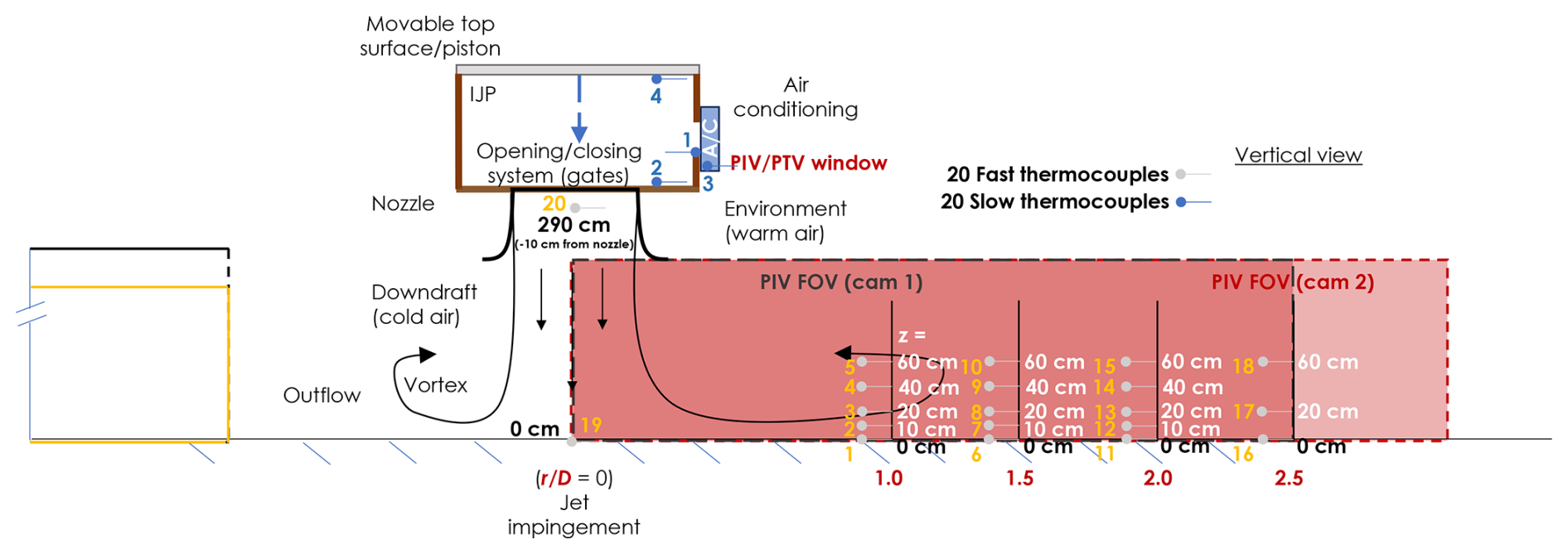
Figure 7 Schematics of measurement setup without orography model installed. Orange and white text in the LS-PIV FOV show the fast-response thermocouple number (Tf #) and its height above the floor. Blue numbers inside the IJP show the standard-response thermocouple numbers (Ts #).

Figure 7 shows a schematic of the experimental setup focused on PIV FOV and thermocouple locations.

For experiments involving the orography model, the 18 fast-response thermocouples were moved to the model surface, specifically along the inner valley and its ridges. Figure 8 provides a schematic representation of the horizontal-plane locations of the thermocouples on the model, while Table 1 lists their corresponding (x, y, z) coordinates. In this notation, x represents the model's longitudinal coordinate, y denotes the transversal direction perpendicular to x, and z indicates the vertical direction (positive upward) from the model surface. The coordinates $(x,y)=(\mathrm{0},\mathrm{0})$ correspond to the southwesternmost point of the model (as shown in Fig. 8), with z=0 indicating a thermocouple placed at the model surface, serving as a relative coordinate reference to account for variations in the model's surface elevation. Key locations, such as the San Giorgio Bridge (formerly known as the Morandi Bridge, thermocouples Tf #3, #8, #9, #10 in Fig. 8 and Table 1) and Erzelli Hill (thermocouple Tf #4 in Fig. 8 and Table 1), were monitored to investigate the effects of flow channeling on temperature evolution within the valley. This setup also aimed to assess the potential development of heat/cool islands due to the trapping of airflow by the surrounding orography. Two additional thermocouples (#9 and #12) were elevated using a suspended horizontal bridge-like wire to measure temperature variations at approximately the height of the San Giorgio Bridge's deck and at a downstream location. Thermocouples #5 and #6 were relocated from experiment #50 as shown in Fig. 8 and Table 1. Thermocouples #19 and #20 were retained at their previous positions, along the vertical centerline of the jet, consistent with the experiments without the model.

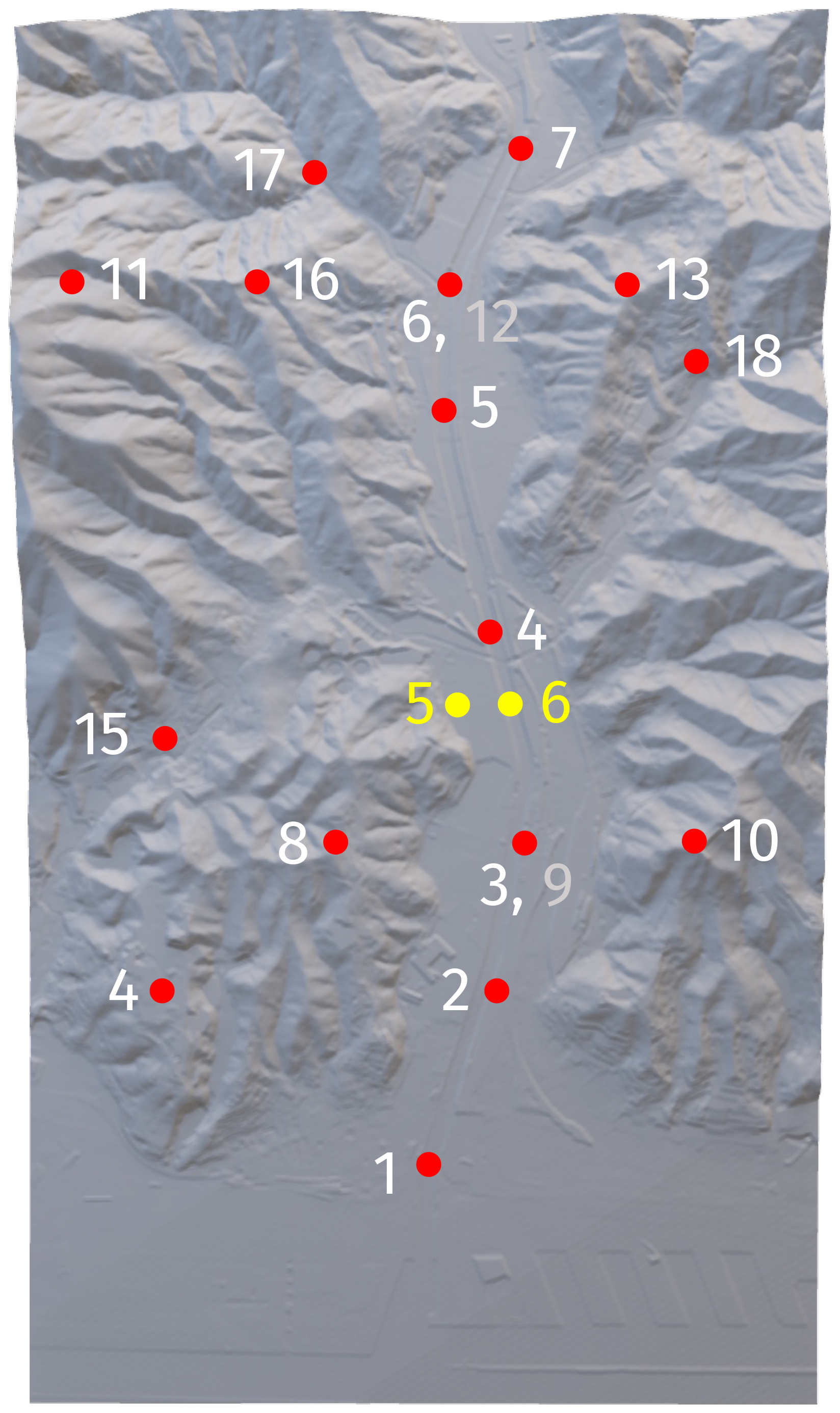
Figure 8 Top view of the three-dimensional stereolithography (STL) orography with indication of thermocouple Tf locations. Grey numbers are thermocouples installed at elevated heights above the model's surface. Yellow numbers are relocated thermocouples from experiment #50.

Table 1 (x, y, z) coordinates of thermocouples Tf on the model.

^* Thermocouples #5 and #6 were relocated from experiment #50. New locations are in brackets.

To relate the 2D horizontal locations of the sensors to the geometric center of the downburst impingement, a simple coordinate transformation can be applied, yielding the new thermocouple coordinates:

$$\begin{array}{}\text{(6)}& {\displaystyle }\begin{array}{rl}& x_{\mathrm{DB}}=x-\mathrm{0.3}\left[\mathrm{m}\right]\left(\mathrm{pos}\mathrm{1}\right)\\ & x_{\mathrm{DB}}=x+\mathrm{0.3}\left[\mathrm{m}\right]\left(\mathrm{pos}\mathrm{2}\right)\end{array}\text{(7)}& {\displaystyle }{y}_{\mathrm{DB}}=y-\mathrm{1.0}\left[\mathrm{m}\right].\end{array}$$

3.5 Test plan

A total of 57 experimental runs were conducted during the campaign at JVCWT. The first 39 experiments focused on recording downburst-like flow fields without the orography model installed, while the final 18 experiments were carried out with the model in place. The test cases varied based on several key parameters, including the temperature difference between IJP and testing chamber prior to the jet release (ΔT), the mechanical impinging-jet velocity (w_IJ), the position of the model when installed (designated as pos#), and repetition number (designated as rep#). A comprehensive list of the experimental runs is provided in Table 2 below. The total number of experiments was reduced compared to the initial test plan, with adjustments made during the campaign due to technical difficulties and specifications related to the experimental setup. These challenges required idle time between consecutive runs. Specifically, achieving a uniform temperature in the large JVCWT chamber proved to be particularly challenging, similarly to maintaining temperature homogeneity within the 8 m³ volume of the IJP.

Table 2 Experimental plan: test case name; chamber (thermocouple #19) temperature before IJ launch at z=0 m above floor, T_WT,Tf19; chamber (thermocouple #20) temperature before IJ launch at z=2.90 m above floor, T_WT,Tf20; IJP temperature before IJ launch in proximity of IJP bottom surface, T_IJP,Ts2; IJP temperature before IJ launch in proximity of IJP top surface, T_IJP,Ts4; Average chamber temperature ($(T_{\mathrm{WT},\mathrm{Tf}\mathrm{19}}+T_{\mathrm{WT},\mathrm{Tf}\mathrm{20}})/\mathrm{2}$), T_WT; Average IJP temperature ($(T_{\mathrm{IJP},\mathrm{Ts}\mathrm{2}}+T_{\mathrm{IJP},\mathrm{Ts}\mathrm{4}})/\mathrm{2}$), T_IJP; Temperature difference between chamber and IJP (T_WT−T_IJP), ΔT; piston velocity, w_p; Theoretical IJ velocity at the impingement region based on w_p (Eq. 5), w_IJ; Theoretical buoyant-jet velocity at the impingement region, w_B (Eq. 3); Theoretical total jet velocity at the impingement region, $w=w_{\mathrm{IJ}}+w_{\mathrm{GC}}$; Richardson number, Ri (Eq. 4). Experimentally-computed average total jet velocity, w_exp; Experimentally-computed Richardson number, Ri_exp.

^a Only 61 samples (corresponding to 5 s) of PIV velocity data were recorded for experiment i010, due to a PIV software error. ^b Only temperature data were recorded for experiment i045, due to a PIV software error. ^c 357 (out of 360) PIV velocity samples were recorded for experiments i050 and i051.

During the initial phase of the campaign, experiments without the model included tests conducted with three temperature differences: ΔT=0, 10, and 20 °C (for w_IJ=1.3 m s⁻¹ only) or 25 °C (for w_IJ=0.8 m s⁻¹ only). However, for the tests with the orography model, the conditions were simplified to just two temperature differences: ΔT=0 and 20 °C. The number of experimental repetitions varied as well; we initially aimed for eight repetitions per test case, but this was later reduced based on time constraints. For the model tests, only two experimental repetitions were performed.

Unlike standard fluid mechanics experiments that typically involve many runs to achieve statistical characterization, each experiment in this campaign must be regarded as unique. This uniqueness arises from variations in parameters among repetitions of the same test case. Controlling and stabilizing variables such as the IJP and chamber air temperatures, the resulting temperature difference (ΔT), the piston release velocity and consequent mechanical impinging-jet velocity (w_IJ) proved challenging. Specifically, as the ΔT between the IJP and the chamber air increases, the temperature uniformity within the IJP decreases. The actual values of these parameters are presented in Table 2, derived from the experimental measurements as outlined in Sect. 4.

4 Database description

The database of experimental signals described in this paper is available in open-access form, provided by Canepa et al. (2025a). It consists of two zip files uploaded to the Zenodo public repository: one containing the LS-PIV data and the other comprising the temperature data.

The PIV zip file, labeled as “PIV.zip”, contains 57 folders, each corresponding to a single experiment. The first 39 folders pertain to the phase of the campaign without the orography model, while the subsequent folders (experiments #40 to #57) relate to tests conducted with the model installed. Each folder is named following the nomenclature outlined under “Test case name” in Table 2: “i0AB_dTCD_VpEF_repG”. Here, AB denotes the experiment number #, CD represents the temperature difference (ΔT) between the IJP and the chamber, EF indicates the impinging-jet velocity derived from the mechanical piston course (where E is the integer part and F is the decimal part, in m s⁻¹), and G is the repetition number #. For experiments involving the orography model, namely experiments #40 to #57, the position of the model is also included in the folder name, formatted as: “i0AB_dTCD_VpEF_posH_repG”, where H is either 1 or 2, indicating the model's position relative to the jet impingement, as shown in Fig. 6, respectively.

Inside each folder, the tab-delimited .txt files correspond to specific time frames of the PIV measurements. Folders for experiments #1 to #15 contain 210 text files (ranging from “V0001.dat” to “V0210.dat”), reflecting 30 s of data recorded at a 7 Hz acquisition frequency. Folders for experiments #16 to #57 contain 360 text files (from “V0001.dat” to “V0360.dat”), representing 30 s of data collected at a 12 Hz acquisition frequency. The first file corresponds to measurements recorded at the time t=0 of nozzle opening. As a reminder, the piston descent began 1000 ms (1 s) after the nozzle opening. Each .txt file comprises various variables extracted from the raw PIV measurements, organized into 8 columns: the longitudinal coordinate r (“r”) [mm]; the vertical coordinate z (“z^′′) [mm]; the horizontal wind speed u (“u^′′) [m s⁻¹], measured as positive in the outgoing direction of downburst propagation; the vertical wind speed w (“w”) [m s⁻¹], measured as positive upward; the correlation value between point(s) in consecutive frames that determine the resulting velocity vector (“Correlation value”); uncertainty quantification of u (“Uncertainty” u); uncertainty quantification of w (“Uncertainty w”); a data validity flag (“isValid”). The uncertainty quantification for velocity components is derived from mapping back two consecutive interrogation windows based on the computed displacement vector field. The original and reconstructed images do not align perfectly, resulting in a non-symmetric correlation peak that indicates the location mismatch. By statistically analyzing how each pixel contributes to the shape of the cross-correlation peak, the uncertainty of the displacement vector can be derived (Wieneke, 2015). Finally, a validity flag is provided for each vector (isValid = 0 for invalid data and 1 for valid data).

The second zip file, named “T.zip”, contains 57 text files, each corresponding to an experimental run and named according to the PIV folder structure defined earlier. Each file records the temperature values from the thermocouples installed as per Figs. 7 and 8, and Table 1 at each sampling time. Files for experiments #1 to #19 include 421 rows (representing sampling times of 30 s at a 14 Hz frequency plus nozzle opening time t=0), while files for experiments #20 to #57 contain 361 rows (30 s at a 12 Hz frequency plus nozzle opening time t=0). Analogously to LS-PIV records, the first measurement of each file corresponds to the opening time of the nozzle, t=0. Each file consists of 28 columns containing the following variables: sample time (“Time”) [s]; temperature “T,wt” [°C], relative humidity “RH,wt” [%], and atmospheric pressure “Patm,wt” [hPa] from a sensor located upstream of the test section inside the main JVCWT horizontal nozzle; temperatures from the “fast” thermocouples labeled “Tf01” to “Tf20” [°C]; and readings from the monitoring “standard” thermocouples labeled “Ts01” to “Ts04” [°C] (as detailed in Sect. 3.4.2). Although each experiment name includes the target ΔT value for that set of tests, the actual value reported in Table 2 is based on the corresponding thermocouple readings at time t=0, marking the opening of the nozzle louvers.

All data files are stored in plain-text tab-delimited format (.txt), which ensures long-term accessibility and compatibility with a wide range of post-processing tools such as MATLAB, Python (pandas, NumPy), R, and common spreadsheet applications. Metadata describing the dataset structure, variable names, and experimental conditions are available on the metadata webpage of the Zenodo repository (https://doi.org/10.5281/zenodo.14609848, Canepa et al., 2025a). Variable names follow concise, self-descriptive labels consistent across all experiments, and all quantities include SI units in the header row of each file. The file-naming convention, as outlined above, encodes the experiment number and the governing parameter values specific to each experiment, thereby facilitating automatic data parsing. While the dataset is distributed as text files for transparency and simplicity, the structure is readily convertible to standard self-describing formats such as NetCDF or HDF5, enabling easy integration with community tools and workflows for fluid dynamics and atmospheric research.

5 Flow and data visualization

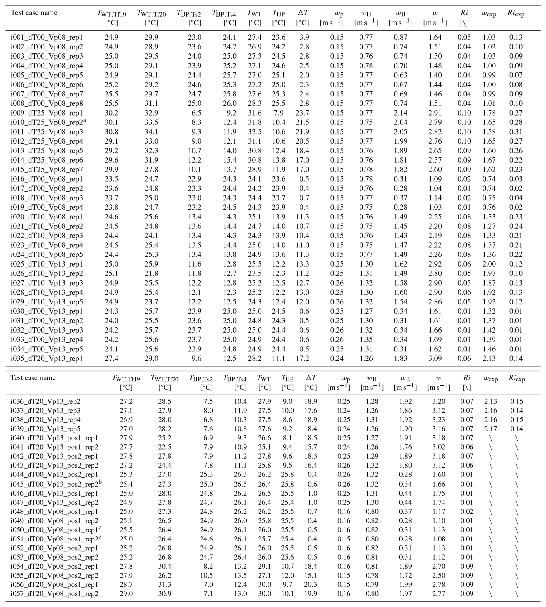
For 12 configurations (all except configurations with model in place ΔT=20 °C, w_IJ=0.8 m s⁻¹, pos 1, and ΔT=20 °C, w_IJ=1.3 m s⁻¹, pos 2), a visualization of the downburst illuminated by two white light LED bars was recorded by a video camera. The experimental setup, including the seeding particles, remained consistent with the standard LS-PIV tests. Figure 9 presents the flow visualizations alongside the corresponding LS-PIV reconstruction of the velocity field in two distinct scenarios: (i) during the downward jet phase near the impingement region (without model) (Fig. 9a and b), and (ii) during the outflow stage with the model positioned at pos (2) (Fig. 9c and d).

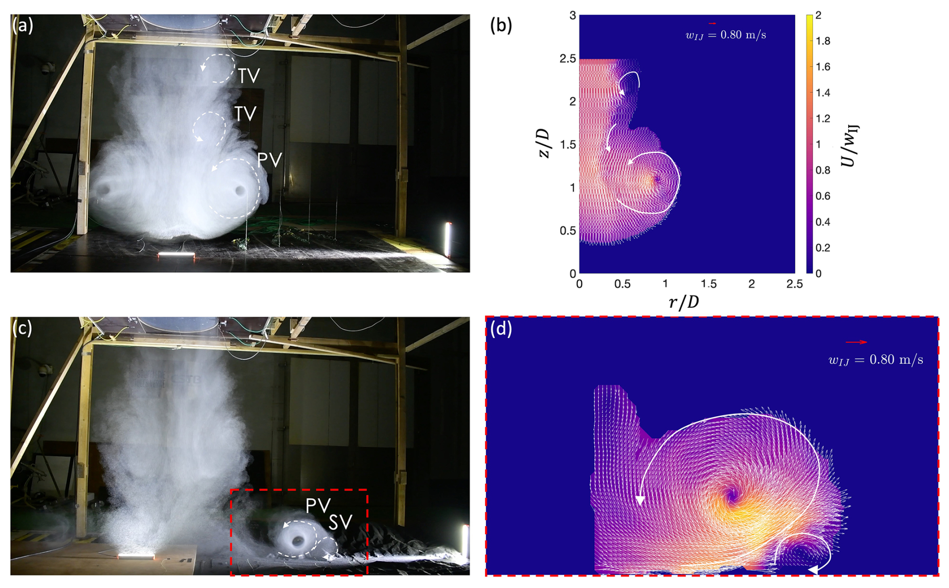
Figure 9 Flow visualization (a, c) and corresponding LS-PIV analysis (b – experiment i016, d – experiment i053) of the velocity flow field at two stages: the near-impingement stage without the model (a, b), and the outflow stage with the model in pos (2) (c, d). (d) Zoom-in of the frontal zone (red rectangle in c). Schematics of vortices (not-to-scale; see Fig. 1) are superimposed to the figures. Both cases have parameters w_IJ=0.8 m s⁻¹ and ΔT=0 °C (see Table 2 for actual values of w_IJ and ΔT).

Figure 10 illustrates the effect of different initial ΔT between the chamber and IJP – specifically ΔT=0 °C (Fig. 10a) and 20 °C (Fig. 10b) (see Table 2 for actual values of ΔT) – on the downburst outflow (Fig. 10a and b), captured at the same time instant after nozzle opening. The temperature variation (in percentage) recorded by thermocouples installed at the surface are also shown for the case ΔT=20 °C (Fig. 10c).

Figure 10 LS-PIV velocity flow field for w_IJ=1.3 m s⁻¹, without the model installed, and (a) ΔT=0 °C (experiment i031) and (b) ΔT=20 °C (experiment i036) (see Table 2 for actual values of w_IJ and ΔT), both captured at t=5.50 s after nozzle opening. (c) Temperature percentage reduction, $-(T_{\mathrm{WT}}-T_i)/T_{\mathrm{WT}}$, where T_i is the temperature at the ith thermocouple (circles in b) and T_WT the chamber temperature at t=0 (before the jet release), for the case i036 (b). Vertical dashed line marks the time t=5.50 s + 0.5 s (thermocouple reaction time).

6 Data availability

The data presented and described in this study are openly available in the Zenodo repository at https://doi.org/10.5281/zenodo.14609848 (Canepa et al., 2025a). Data can be further reused under Creative Commons license CC0 for metadata and CC-BY for data.

7 Conclusions and perspectives

This paper presents a dataset of 57 experiments carried out at the Jules Verne Climatic Wind Tunnel (JVCWT) of the CSTB laboratory in Nantes, France, as part of the European-funded ERIES-CLIMATHUNDERR project – CLIMAtic investigation of THUNDERstorm winds. The study addresses the evolution of flow velocity and temperature fields during the occurrence of downburst-like winds, focusing on the effects of varying temperature differences between the recreated buoyant impinging jet and the calm ambient air prior to jet release. The experimental techniques used include Large-Scale Particle Image Velocimetry (LS-PIV) for recording velocity fields and thin thermocouples for temperature values. For the first time, downburst winds were recreated at a large geometric scale using a combination of the traditionally employed mechanical impinging jet and gravity current methods. While matching all dimensionless parameters (e.g., the Reynolds number, Re) between scaled experiments and full-scale events is inherently impossible, the presented database, by focusing on the Richardson number (Ri) and large-scale flow structures, is expected to offer new insights into the influence of temperature on the overall geometry and dynamics of downburst outflows. It will enable an evaluation of how the intensity of a downburst varies based on the temperature differential with the surrounding environment, and thus its potential impact on both natural and built environments. Full-scale recordings of downburst events, including wind speed and temperature data, primarily come from the database of downburst events collected by the GS-WinDyn Research Group at the University of Genoa, in the main ports of the Northern Mediterranean Sea (De Gaetano et al., 2014; Burlando et al., 2018; Canepa et al., 2020, 2024b), as well as from external databases (e.g., Lombardo et al., 2009). These data will allow for a statistical comparison with the experiments described here. This database will serve as a new benchmark for calibrating and validating numerical and analytical models of downburst winds. The inclusion of temperature as a new variable in the governing equations describing downbursts will lead to a more refined model of the phenomenon, which can be incorporated into building codes and wind loading guidelines. We anticipate that this dataset will be valuable to a broad range of fields, including atmospheric physics, meteorology, climatology, fluid dynamics, natural and multi-risk disaster modeling, as well as for insurance companies.