StageIV-IRC: a high-resolution dataset of extreme orographic Quantitative Precipitation Estimates (QPE) constrained to water budget closure for historical floods in the Appalachian Mountains

Quantitative Flood Estimation (QFE) in complex terrain remains a grand challenge in operational hydrology due to the lack of accurate high-resolution Quantitative Precipitation Estimates (QPE) for operational forecasting and for calibrating hydrologic models. Here, we present a high-resolution (i.e., 250 m, 5 min-hourly) QPE dataset for 215 extreme rainfall events occurred in 26 gauged mountainous basins in the Appalachian Mountains from 2008 to 2024. This dataset is developed by applying inverse rainfall corrections (IRC) derived from physically-based rainfall-runoff modeling (Liao and Barros, 2022 and 2023) to the Next Generation Weather Radar (NEXRAD) Stage IV analysis (4 km resolution, hourly). The corrected Stage IV analysis QPE is referred to as StageIV-IRC (StageIV with Inverse Rainfall Correction). The unique advantage of this StageIV-IRC QPE dataset is its agreement with ground-based rainfall measurements while achieving water budget closure at the storm-flood event scale and minimizing uncertainty from initial conditions using the Initial Condition Correction (ICC) module. This dataset is the first QPE dataset aiming to improve QFE in the complex terrain by reducing biases for extreme precipitation events, and it can be used to evaluate the skill of hydrologic models in the same basins and support model calibration. The StageIV-IRC QPE dataset is publicly available at https://doi.org/10.5281/zenodo.14028866 (Liao and Barros, 2025c), and improved initial soil moisture maps for the studied extreme precipitation events, derived from the ICC module in the same IRC framework, are available in the same repository.

1 Introduction

Over the past few decades, extreme precipitation has become an increasingly important research topic due to its social, economic, and environmental impacts (e.g., Alimonti et al., 2022; Wernberg et al., 2013). Studies show that both total annual precipitation and extreme precipitation events have increased in the US and in other parts of the world during the last century (e.g., Milly et al., 2002), often resulting in floods (e.g., Pielke et al., 2002), and flash floods in the context of complex terrain due to steep slopes (e.g., Schumacher, 2017; Czigány et al., 2010). Flash floods are characterized by fast rainfall-runoff responses on the scale of a few hours (< 6 h) after extreme precipitation events for watershed areas often ranging from a few tens to hundreds of square kilometers (e.g., Borga et al., 2014; Lumbroso and Gaume, 2012). As one of the deadliest natural hazards, flash floods are often associated with landslide events (e.g., Tao and Barros, 2014; Gupta et al., 2016; Deijns et al., 2022) and cause loss of life and property damage (Špitalar et al., 2014), such as recently in the last three years in the Appalachian Mountains, USA, and in Southern Spain. Despite extensive studies to improve flash flood simulations in small headwater basins, hydrological skill scores (e.g., Kling-Gupta Efficiency or KGE) remain poor at event scales largely due to significant difficulties involved in estimating highly localized orographic precipitation in complex terrain, which in turn implies that hydrologic models are not calibrated using forcing representative of realistic extreme events (e.g., Andrieu et al., 1997; Huffman et al., 2007; Mtibaa and Asano, 2022).

Current approaches involved in precipitation measurement and Quantitative Precipitation Estimation (i.e., QPE) broadly include in-situ point-scale observations using rain gauges and disdrometers, and remote spatial observations using ground-based radar and space-based sensors. In complex terrain, there is often a scarcity of in situ measurements due to difficult access. For example, the rain gauge network from NASA's Integrated Precipitation and Hydrology Experiment is the only relatively dense rain gauge network installed at high elevations in the entire Appalachians (e.g., Barros et al., 2014). Other QPE products (e.g., radar QPE data) are plagued by uncertainties from various sources (e.g., ground clutter artifacts, retrieval uncertainties, and radar viewing geometry (Villarini and Krajewski, 2010; Arulraj and Barros, 2021; Kreklow et al., 2020; Huffman et al., 2007; Andrieu et al., 1997; Durden et al., 1998). Numerical weather prediction (NWP) is an alternative to measurement. However, QPE products from NWP models are characterized by significant uncertainties when evaluated against rain gauges (e.g., Zhang and Anagnostou, 2019), leading to large flood simulation errors when used as inputs to hydrological models, or introducing large structural uncertainty when used for model calibration (e.g., Tao et al., 2016; Weiland et al., 2015; Diomede et al., 2008; Kobold and Sušelj, 2005). Due to these uncertainties and errors involved, focus has been directed towards enhancing QPE using various methods: data merging of raingauge and radar precipitation (e.g., McKee and Binns, 2016; Goudenhoofdt and Delobbe, 2009; Delrieu et al., 2014; Nanding et al., 2015; Sideris et al., 2013; Schiemann et al., 2011), combined radar reflectivity and retrieval corrections (e.g., Vignal et al., 2000; Shao et al., 2021; Dinku et al., 2002), and data assimilation into NWP models (e.g., Rafieeinasab et al., 2015; Wehbe et al., 2020). Rain gauge and disdrometer measurements are often used as references for these QPE optimization approaches (e.g., Harrison et al., 2000; Shao et al., 2021; Fulton et al., 1998). The “ground truth”, however, has its own error (e.g., spatial representativeness, wind artifacts around the gauge orifice, and calibration, among others; Kochendorfer et al., 2017), and fails to capture highly localized orographic enhancement (e.g., Prat and Barros, 2010b; Gentilucci et al., 2021; Buytaert et al., 2006). Gauge-radar fusion often relies on geostatistical assumptions that are primarily distance-based (e.g., Areerachakul et al., 2022; Cassiraga et al., 2021; Wang et al., 2020; Maggioni and Massari, 2018), lacking the full picture of complex basin topography, which has a regulating role in orographic precipitation processes.

To address this long-standing QPE challenge in complex terrain, a general QPE error quantification framework was developed leveraging widely available quality United States Geological Survey (USGS) streamflow observations at the outlet of headwater basins in complex terrain, consisting of 2 distinct paths: (1) rain gauge bias correction, and (2) grid-level QPE correction constrained to watershed-scale water budget closure. The first pathway includes rain gauge bias corrections at gauge locations both at the diurnal and climate scales, and the geostatistical distribution of rain gauge biases across a basin. The second pathway includes an innovative inverse QPE correction method by backward propagating runoff uncertainty using a hydrological model via streamlines to precipitation at storm-event scale, and the methodology is termed Inverse Rainfall Correction (IRC), which is developed by the same authors (Liao and Barros, 2022 or LB22). The IRC was initially developed in the Southern Appalachians and later extended to headwater basins over a span of 2000 km from south to north along the entire Appalachian Mountains. It is worth noting that rain gauges are only available in the Southern Appalachians, thus elsewhere the StageIV product was downscaled to 250 m first and then submitted to the IRC without bias corrections or any other intermediate corrections as in LB22. The generalizability of the IRC framework, regardless of rain gauge bias corrections beforehand, is demonstrated in Liao and Barros (2023).

LB22 found that initial soil moisture uncertainty causes inferior performance of IRC because large initial condition errors lead to significant uncertainties in travel time distributions. Soil moisture is considered a particularly important factor among soil properties due to its significant role in affecting the generation of runoff, hence dramatically altering the timing of flood front and its magnitudes (e.g., Vivoni et al., 2007; Marchi et al., 2010; Penna et al., 2011), and soil moisture can vary dramatically at hourly timescales, changing from fully saturation levels to wilting point levels conditional on the specific texture and other properties of the soils (Grillakis et al., 2016). Initial soil moisture conditions can therefore determine whether a rainstorm produces a major flash flood or not (e.g., Komma et al., 2007; Zehe and Blöschl, 2004). However, due to the limited availability of soil moisture sensors, there are not many studies quantifying the impact of soil moisture on runoff simulation (e.g., Silvestro et al., 2019; Laiolo et al., 2016; Zappa et al., 2011; Uber et al., 2018). Liao and Barros (2025b) developed an Initial Condition Correction (ICC), which is based on travel time distributions and is coupled with the general IRC approach, demonstrating large improvements in initial soil moisture estimation. Note that when implementing the IRC and ICC, we are using a fully distributed physics-based uncalibrated model (i.e. Duke Coupled Hydrological Model, DCHM) that has been used successfully for more than two decades for hydrologic studies in the Southern and Central Appalachians (e.g., Tao and Barros, 2013, 2014, 2018 and 2019; Tao et al., 2016; Yildiz and Barros 2004, 2007 and 2009), and consequently uncertainty from model structure and model parameters is assumed to be small. Hydrological model parameters certainly have an impact on rainfall-runoff response, but they are generally only of secondary importance compared to the precipitation proper and antecedent soil moisture distributions, especially for smaller basins (e.g., Dobler et al., 2012; Mockler et al., 2016).

In this work, IRC and ICC are combined into one framework, referred to as the IRC-ICC framework in Liao and Barros (2025b), to construct an improved QPE dataset aiming to close the water budget at the scale of storm-flood events along the entire Appalachian Mountains range, The study region is set to be the Appalachian Mountains because they are prone to extreme precipitation and flash floods due to orographic lift of moisture-laden air masses coming from the Gulf of Mexico and the Atlantic Ocean (e.g., Troch et al., 1994; Smith et al., 2011; Liao and Barros, 2023). A recent example is Hurricane Helene, which caused over 200 deaths and over USD 50 billion in property damage in the Southeast US in September 2024. The IRC-ICC framework is employed in 26 headwater basins and 215 extreme events (during 2008–2024) using the Next Generation Weather Radar (NEXRAD) StageIV dataset as original inputs, at a spatial and temporal resolution of 250 m and 5 min, respectively, and the improved post IRC-ICC QPE data (i.e., StageIV-IRC) are made available in this study.

The manuscript is organized as follows. The data sources and the QPE error quantification framework, which consists of rain gauge bias correction and the IRC-ICC framework, are detailed in Sect. 2. Section 3 presents this new dataset (StageIV-IRC) along with data assessment from various aspects. Section 4 discusses the potential application of this new dataset and future work. Section 5 provides access to the dataset and a summary of the work.

2 Data and Methodology

2.1 Radar QPE StageIV

The NCEP/EMC StageIV is a precipitation estimation product, developed using hourly and 6-hourly radar-raingauge precipitation analyses at regional scales (Lin and Mitchell, 2005). In complex terrain, it is known that radar QPE suffers from the blockage of topography, overshooting and retrieval uncertainties, leading to large uncertainties in rainfall estimation. In 2007, as part of the ground validation (GV) of the Precipitation Measurement Missions (PMM) program by NASA (e.g., Prat and Barros, 2010a, b), 34 tipping bucket raingauges were installed in the Southern Appalachians and have been well-maintained since 2007 (e.g., Barros et al., 2014). In this work, raingauge measurements from a GV raingauge network are utilized to reduce StageIV uncertainties in the Southern Appalachians.

2.2 GV Rain Gauge Observations

A rain gauge network in support of PMM GV was installed in the Pigeon River basin for the 10 year 2007–2018 period (Barros et al., 2014). A map of this rain gauge network is plotted in Fig. 1. Every rain gauge is labelled with a number, and exact locations are documented in Table 1. This rain gauge network is regularly visited and maintained at least three times a year, including on-site cleaning and calibration. In this study, these rainfall measurements are used as a basis to adjust hourly StageIV QPE. Note these rain gauge measurements can be downloaded at https://doi.org/10.5067/GPMGV/IPHEX/GAUGES/DATA301 (Barros et al., 2017). Besides rain gauges, a network of Parsivel disdrometers was installed during 2013–2014, with each disdrometer location denoted by the letter P in Fig. 1. These disdrometer data were only used for independent evaluation because of short records. It is worth noting that rain gauges are installed mostly along the ridges while disdrometers are generally located at lower elevations.

Table 1 Raingauge index and exact locations as illustrated in Fig. 1. Two rain gauges highlighted in bold font are installed at Purchase Knob, a supersite in the inner mountain region. Locations equipped with more than one raingauge (collocated) are highlighted in italic font, and these collocated raingauges generally differ in tipping sizes. This table is adapted from Liao and Barros (2019).

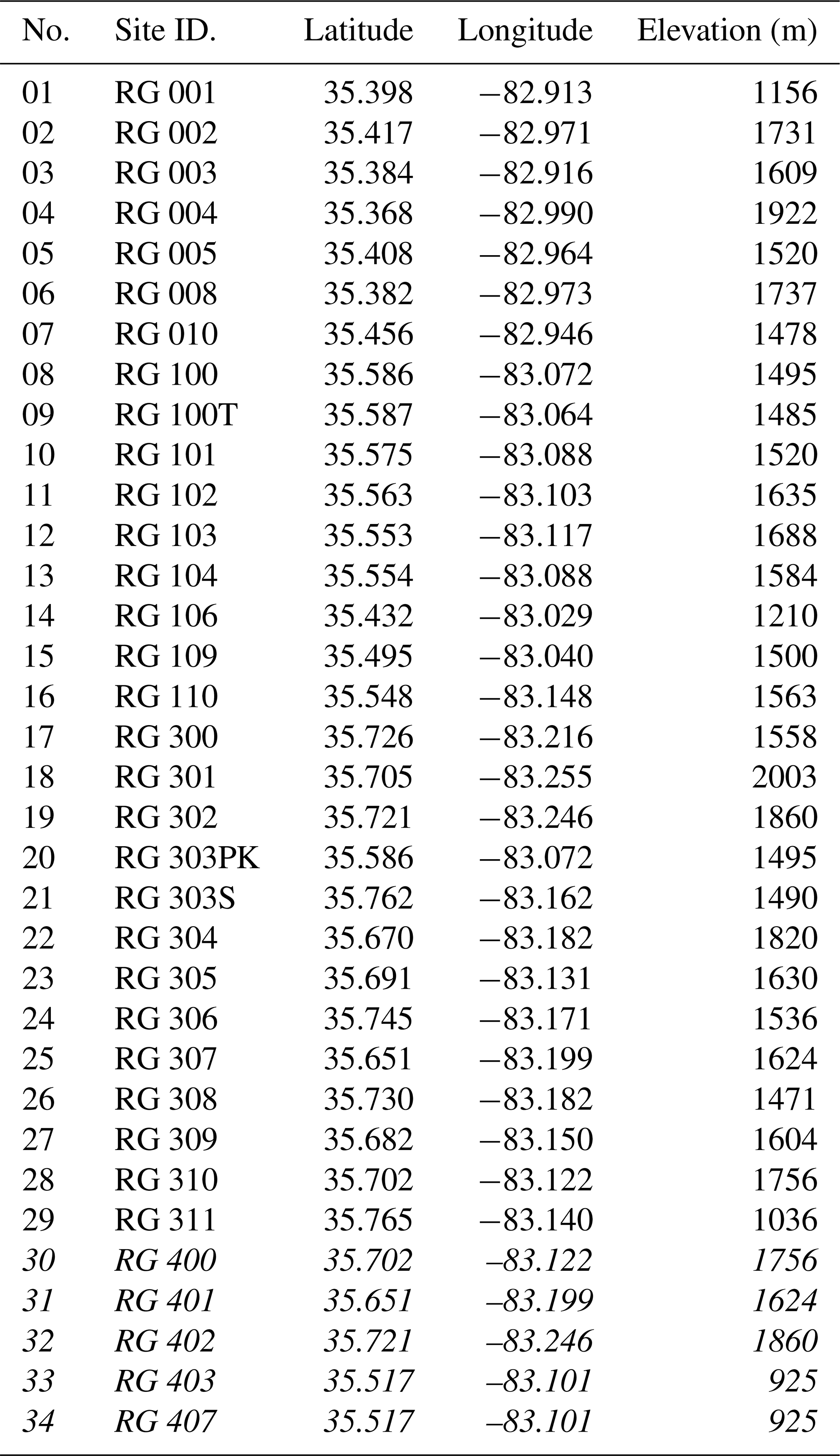
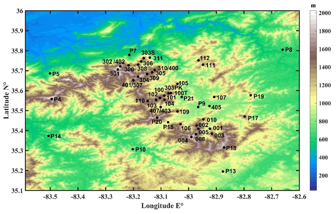
Figure 1 Map of IPHEx (Barros et al., 2014) ground-based observations in the Southern Appalachians. Raingauge is denoted as a character string starting with three-digit number potentially followed by extra letters; locations started with a letter P represent disdrometers. The basic information regarding these stations is listed in Table 1. This figure is adapted from Liao and Barros (2019).

2.3 Methodology

The methodology of this work includes four major elements: (a) rain gauge bias and climatology corrections where raingauge data are available, (b) downscaling of radar precipitation, (c) grid-scale QPE correction by closing the water budget using stream gauge measurements, and (d) basin and event selection procedures and model setup.

2.3.1 Rain Gauge Corrections

A schematic drawing of the rain gauge correction framework to derive gauge-improved QPE (named StageIV_DBKC) is provided in Fig. 2. The subscripts DBKC refer to “Downscaled”, “Bias correction using rain gauge measurements at gauge locations”, “Kriging interpolation in 2D”, and “Climatological corrections”, respectively.

Figure 2 Workflow to generate the product STIV_DBKC.

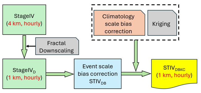
First, to make meaningful comparison between StageIV estimates and rain gauge measurements spatially, a fractal downscaling algorithm is used to create StageIV_D at 1km from the original StageIV at 4 km resolution. Subsequently, bias correction using raingauge measurements is employed to create StageIV_DB at hourly timescales. StageIV_DB data are then evaluated against the rain gauge climatology from 2008 to 2017 to reduce biases that depend on weather regime, and climatological biases are then spatially interpolated using the ordinary Kriging method. The resulting dataset is named StageIV_DBKC (abbreviated as STIV_DBKC).

2.3.2 Fractal downscaling

The methodology for fractal downscaling was first proposed by Bindlish and Barros (1996) and subsequently demonstrated through various applications to precipitation downscaling from models (Bindlish and Barros, 2000) and remote sensing data (Nogueira and Barros, 2015; Tao and Barros, 2010). Here, a brief description is presented.

The assumption of self-similarity is imposed in fractal downscaling approach. The parameters used in this approach involve: fractal dimension D, Hurst coefficient H, and the spectral exponent β that are related through the following equations:

$$\begin{array}{}\text{(1)}& {\displaystyle }D={\displaystyle \frac{\mathrm{7}-\mathit{\beta }}{\mathrm{2}}}\text{(2)}& {\displaystyle }H={\displaystyle \frac{\mathit{\beta }-\mathrm{1}}{\mathrm{2}}}\end{array}$$

The parameter β describes rainfall statistics across different spatial scales, and it is calculated as the slope of the power spectral density curve in the 2D Fourier domain of the rainfall field (log-log plot). The parameter H is the Hurst coefficient which is a measure of autocorrelation strength with higher value representing stronger autocorrelation. The 2D Fourier transform of a rainfall field z(x,y) is calculated as the following:

$$\begin{array}{}\text{(3)}& \begin{array}{rl}Z\left(u,v\right)& ={\left({\displaystyle \frac{L}{N}}\right)}^{\mathrm{2}}\sum _{x=\mathrm{0}}^{N-\mathrm{1}}\sum _{y=\mathrm{0}}^{N-\mathrm{1}}z\left(x,y\right)\\ & \exp \left[-{\displaystyle \frac{\mathrm{2}\mathit{\pi }i}{N}}\left(ux+vy\right)\right]\end{array}\end{array}$$

where N is the total number of grid points of the rainfall field z(x,y) with grid size being the L, u and v correspond to frequency indices in the Fourier domain in each direction. Using Eq. (3), the averaged power spectral density is given:

$$\begin{array}{}\text{(4)}& S_j={\displaystyle \frac{\mathrm{1}}{L^{\mathrm{2}}{N}_j}}\sum _{\mathrm{1}}^{N_j}{\left|Z(u,v)\right|}^{\mathrm{2}}\end{array}$$

where N_j denotes the number of points that meet the following condition: $j<\sqrt{u^{\mathrm{2}}+v^{\mathrm{2}}}<j+\mathrm{1}$. The mean power spectral density and the wavenumber k (Eq. 5) are related by a power law (Eq. 6):

$$\begin{array}{}\text{(5)}& {\displaystyle }k={\displaystyle \frac{\mathrm{2}\mathit{\pi }}{\sqrt{u^{\mathrm{2}}+v^{\mathrm{2}}}}}\text{(6)}& {\displaystyle }S\sim k^{-\mathit{\beta }-\mathrm{1}}\end{array}$$

By applying a logarithmic transformation, the power-law relation between S and k is linearized, and the S value when wavenumber k=1 is the roughness factor, which is a representation of the variance of the field.

Assuming rainfall fields have self-similar statistics expressed by a power-law, then fine scale rainfall fields can be generated from the coarse scale radar observations by preserving these self-similar statistics. This is accomplished by creating a Brownian surface at desired fine scale resolution while sharing the same spectral slope and roughness factor as the original rainfall field based on Bindlish and Barros (1996):

$$\begin{array}{}\text{(7)}& Z_{\mathrm{D}}\left(u,v\right)={\displaystyle \frac{Z_{\mathrm{b}}\left(u,v\right)}{k_{\mathrm{r}}^{\left(\mathit{\beta }-{\mathit{\beta }}_{\mathrm{b}}\right)/\mathrm{2}}}}\exp \left[{\displaystyle \frac{\mathrm{1}}{\mathrm{2}}}\left(S_{\mathrm{r},\mathrm{1}}-{\displaystyle \frac{\mathit{\beta }+\mathrm{1}}{{\mathit{\beta }}_{\mathrm{b}}+\mathrm{1}}}{S}_{\mathrm{r},\mathrm{2}}\right)\right]\end{array}$$

where β, β_b, Z_D(u,v) and Z_b(u,v) are the spectral slope of 2D original rainfall field, the spectral slope of the Brownian surface, interpolation surface in the Fourier domain and original Brownian surface, respectively; k_r is the wavenumber and S_r,1 and S_r,2 are the roughness factors of the 2D original rainfall fields and Brownian surface. Due to the non-uniqueness of Brownian surfaces, multiple replicates of interpolation surfaces Z_D must be generated. In this study, an ensemble of ND (Number of Downscaled samples) interpolation surfaces is derived from the original StageIV product where ND = 50 following Nogueira and Barros (2015), and thus fifty rainfall field realizations at finer resolution preserving the same rainfall statistics at coarse resolution is generated, and the ensemble mean was calculated. Finally, the rainfall correction steps described in Fig. 2 are applied to the ensemble mean of the downscaled rainfall fields.

2.3.3 Climatology Corrections

The first phase of bias correction is carried out at the event scale: a linear regression is established between rain gauge measurements and collocated downscaled radar pixel estimates using the following formula:

$$\begin{array}{}\text{(8)}& R_{\mathrm{g}}^t\left(i_{\mathrm{g}},j_{\mathrm{g}}\right)=\mathit{\kappa }{R}_{\mathrm{r}}^t\left(i_{\mathrm{g}},j_{\mathrm{g}}\right)+\mathit{\epsilon }\end{array}$$

where R_r and R_g represent radar and rain gauge measurements respectively, κ and ε are the slope and the intercept of a polynomial fit between R_r and R_g. Hourly StageIV_D estimates and corresponding rain gauge observations in the same StageIV_D pixel were identified if at least 2 rain gauges in the same StageIV_D pixel measure non-zero rainfall. A linear regression was applied to all StageIV_D pixels within one standard deviation of the regression line at an hourly timescale by assuming homogeneity of variances or homoscedasticity.

The second phase of bias correction is done at decadal scale: aiming to reduce systematic radar errors caused by retrieval uncertainties and viewing geometry in complex terrain, demonstrating strong diurnal (time of day) and seasonal (weather regime) error dependencies due to missed detection of shallow rainfall systems related to radar overshooting in the Southern Appalachian when comparing against 10-year rain gauge observations (e.g., Prat and Barros, 2010b; Wilson and Barros, 2014; Duan et al., 2015). For this purpose, when rain gauge observations are < 2 mm h⁻¹ and Stage IV_D estimates are 0 mm h⁻¹, the StageIV_D value was automatically replaced by the rain gauge observations, which is referred to as the Light Rainfall Correction (LRC). Moreover, if StageIV_D rainfall intensity is zero where at least one collocated rain gauge observation is > 2 mm h⁻¹, then StageIV_D estimates are replaced by the mean of all collocated rain gauge observations, namely Mean Rainfall Correction (MRC). Lastly, for highly localized precipitation (i.e., fewer than 2 rainguages register nonzero rain in the study domain) which is normally associated with small-scale convective activity, the rainfall differences between the StageIV_D and the local rain gauge observations were bilinearly distributed across nearby grids (a 5×5 grid square centered at the StageIV_D pixel) – Convective Rainfall Correction (CRC). For most of the raining hours, there are more than 2 rain gauges with nonszero rainfall, in which case the differences between radar estimates and raingauge measurements were spatially interpolated using ordinary Kriging, which is refered to as the Global Rainfall Correction (GRC).

2.3.4 Ordinary Kriging

Ordinary Kriging is a geostatistical interpolation method that generates artificial values of a variable at a specific location, aiming to minimize spatial variance. In this work, rainfall differences between raingauge observations and StageIV_DB are calculated and distributed across the entire basin using a spatial variance model, which is commonly referred to as a semi-variogram model. Specifically, a spherical semi-variogram model is used. Literature regarding the choice of semi-variogram models and their properties can be found (e.g., Li and Heap, 2008; Oliver and Webster, 2015; Zimmerman and Zimmerman, 1991). Bohling (2005) pointed out that spherical models reach the maximum variance for relatively shorter spatial lags, therefore more suitable to capture highly nonlinear and localized orographic precipitation (McBratney and Webster, 1986):

$$\begin{array}{}\text{(9a)}& {\displaystyle }\mathit{\gamma }\left(h\right)=C_{\mathrm{0}}+\left(C-C_{\mathrm{0}}\right)\left({\displaystyle \frac{\mathrm{3}h}{\mathrm{2}d}}-{\displaystyle \frac{\mathrm{1}}{\mathrm{2}}}{\left({\displaystyle \frac{h}{d}}\right)}^{\mathrm{3}}\right)\text{if}\mathrm{0}\le h\le d\text{(9b)}& {\displaystyle }=C\text{ if }h>d\text{(9c)}& {\displaystyle }{\mathit{\gamma }}_{\mathrm{0}i}={\displaystyle \frac{\mathrm{1}}{N_A}}\sum _{k=\mathrm{1}}^{N_A}{\mathit{\gamma }}_{ki}\text{(9d)}& {\displaystyle }{\mathit{\gamma }}_{\mathrm{00}}={\displaystyle \frac{\mathrm{1}}{N_A}}\sum _{k=\mathrm{1}}^{N_A}\sum _{l=\mathrm{1}}^{N_A}{\mathit{\gamma }}_{kl}\end{array}$$

where h is the lag, d is the range, C and C₀ are the sill and nugget values of the semi-variogram model, N_A is the number of raingauges. The nugget is assumed to be zero if local variability and measurement error are neglected at the point scales (Diggle and Ribeiro, 2007). The interpolated rainfall difference at a location $x_{\mathrm{0}}{Z}_{\mathrm{ok}}^{\ast }\left(x_{\mathrm{0}}\right)$ is calculated using a weighted combination of all available differences at gauge locations G(x_i) multiplied by Ordinary Kriging weights ${\mathit{\lambda }}_i^{\mathrm{ok}}$:

$$\begin{array}{}\text{(10a)}& {\displaystyle }{Z}_{\mathrm{ok}}^{\ast }\left(x_{\mathrm{0}}\right)=\sum _{i=\mathrm{1}}^n{\mathit{\lambda }}_i^{\mathrm{ok}}G\left(x_i\right)\text{(10b)}& {\displaystyle }\sum _{i=\mathrm{1}}^n{\mathit{\lambda }}_i^{\mathrm{ok}}=\mathrm{1}\end{array}$$

Optimal Kriging weights can be obtained by a series of linear equations using the Lagrange multiplier μ method:

$$\begin{array}{}\text{(11)}& \begin{array}{rl}& \left(\begin{array}{cc}\begin{array}{ccc}{\mathit{\gamma }}_{\mathrm{11}}& \mathrm{\dots }& {\mathit{\gamma }}_{n\mathrm{1}}\\ \mathrm{⋮}& \mathrm{\ddots }& \mathrm{⋮}\\ {\mathit{\gamma }}_{\mathrm{1}n}& \mathrm{\cdots }& {\mathit{\gamma }}_{nn}\end{array}& \begin{array}{c}\mathrm{1}\\ \mathrm{⋮}\\ \mathrm{1}\end{array}\\ \begin{array}{ccc}\mathrm{1}& \mathrm{\cdots }& \mathrm{1}\end{array}& \mathrm{0}\end{array}\right)\left(\begin{array}{c}{\mathit{\lambda }}_{\mathrm{1}}^{\mathrm{OK}}\\ \mathrm{⋮}\\ \begin{array}{c}{\mathit{\lambda }}_n^{\mathrm{OK}}\\ \mathit{\mu }\end{array}\end{array}\right)\\ & =\left(\begin{array}{c}{\mathit{\gamma }}_{\mathrm{01}}\\ \mathrm{⋮}\\ \begin{array}{c}{\mathit{\gamma }}_{\mathrm{0}n}\\ \mathrm{1}\end{array}\end{array}\right)\end{array}\end{array}$$

In this work, Ordinary Kriging interpolates differences between radar data and raingauge observations to produce gauge-corrected STIV_DBKC dataset. An example sequence of rainfall fields to illustrate the step-wise corrections described in Sect. 2.3.1–2.3.4 is shown in Fig. A1.

2.3.5 Precipitation Assessment Metrics

Assessment metrics include the following: bias and root mean square error between radar estimation and raingauge measurement, false alarm rate, the probability of detection (PD), threat score (TS) and Heidlke skill score (HSS), following McBride and Ebert, 2000. An instance when both radar QPE and rain gauge observation exceed a specified rain rate threshold is a hit (H); when observation matches the criterion and radar QPE does not, it is classified as a miss (M); if the opposite happens, then it is a false alarm (FA). The calculation of these metrics relied on a collection of Hs, Ms, and FAs:

$$\begin{array}{}\text{(12)}& {\displaystyle }\mathrm{Bias}={\displaystyle \frac{\mathrm{1}}{N}}\sum _{n=\mathrm{1}}^N\left(O_n-R_n\right)\text{(13)}& {\displaystyle }\mathrm{RMSE}=\sqrt{{\displaystyle \frac{\mathrm{1}}{N}}\sum _{n=\mathrm{1}}^N{\left(O_n-R_n\right)}^{\mathrm{2}}}\text{(14)}& {\displaystyle }\mathrm{FR}={\displaystyle \frac{\mathrm{FA}}{\mathrm{H}+\mathrm{FA}}},\mathrm{0}\le \mathrm{FR}\le \mathrm{1}\text{(15)}& {\displaystyle }\mathrm{PD}={\displaystyle \frac{\mathrm{H}}{\mathrm{H}+\mathrm{M}}},\mathrm{0}\le \mathrm{PD}\le \mathrm{1}\text{(16)}& {\displaystyle }\mathrm{TS}={\displaystyle \frac{\mathrm{H}}{\mathrm{H}+\mathrm{FA}+\mathrm{M}}},\mathrm{0}\le \mathrm{TS}\le \mathrm{1}\text{(17)}& {\displaystyle }\begin{array}{rl}\mathrm{HSS}& =\mathrm{2}\cdot {\displaystyle \frac{Z\cdot \mathrm{H}-\mathrm{FA}\cdot \mathrm{M}}{\left(\left(H+\mathrm{FA}\right)\cdot \left(Z+\mathrm{FA}\right)\right)+\left(\left(\mathrm{M}+\mathrm{H}\right)\cdot \left(\mathrm{M}+Z\right)\right)}},\\ & -\mathrm{1}\le \mathrm{HSS}\le \mathrm{1}\end{array}\end{array}$$

where O is the rain gauge observation, R is the radar QPE, and N is the number of points. Z represent the number of zeros, meaning both raingauge and radar do not register a rainfall record above a predefined threshold. A threat score (TS) of 0.5 means over 50 % of cases meet the criterion, and the higher the better. An HSS of 0 means a forecast has the same performance as a random guess.

2.3.6 Inverse Hydrologic Correction

At flash flood timescales in headwater basins, streamflow uncertainty and precipitation uncertainty are strongly connected in a nonlinear way through rainfall runoff processes. Liao and Barros (2022) developed a Lagrangian-based framework named Inverse Rainfall Correction (IRC), allowing backpropagating streamflow uncertainty to precipitation inputs in space and time through an uncalibrated distributed hydrological model (i.e., DCHM), achieving water budget closure at the event scale in small headwater basins. As stated earlier, the uncertainties associated with parameters and the hydrological model DCHM are neglected since the model configurations have been used and improved over the past two decades for this region accounting for various soil, vegetation, and river processes (e.g., Tao and Barros, 2013, 2014, 2018 and 2019; Yildiz and Barros, 2007; Lowman and Barros, 2016), and the IRC framework has been tested in multiple headwater basins extensively in this region with consistent success. The detailed description of the IRC is provided in Sect. 2.3.8 and Appendix A.

It is worth noting that IRC is a general framework to improve QPE at the watershed scale that can be incorporated into any distributed hydrological models. Liao and Barros (2025a, b) investigated the impact of model structure uncertainty and initial condition uncertainty on IRC and then the downstream product the resulting IRC improved QPE. The results suggest with improved watershed physics at finer resolution (e.g., river bank storage, Liao and Barros, 2025a), river routing algorithms (e.g., XY routing, Liao and Barros, 2025a) and improved antecedent soil moisture distributions (Liao and Barros, 2025b), post-IRC QPE demonstrate realistic precipitation features at high resolution that are aligned with basin topography with ridges associated with higher precipitation than valleys in general, showing a significant improvement from the original StageIV dataset which is characterized by unnatural boxy precipitation patterns in complex terrain due to resolution issues and over or underestimation depending on topography and distance from the radar site.

As briefly mentioned before, LB22 reviewed various sources of uncertainty that can prevent post-IRC QPE from achieving water budget closure, among which initial condition uncertainty in soil moisture is a noteworthy source. Improved initial condition estimation results in significantly improved post-IRC precipitation features in complex terrain by better capturing transient travel time distributions (Liao and Barros, 2025b). They found that the uncertainty tied to initial conditions is more significant for less extreme events. Nevertheless, the initial condition correction method is coupled with the IRC framework, and the complete framework is named the IRC-ICC framework. The specifics regarding the IRC, ICC, and IRC-ICC are schematically drawn in Fig. 3.

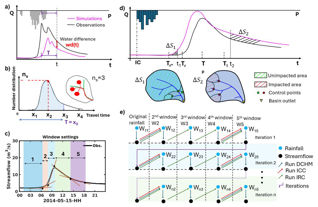
Figure 3 An illustration of the structure of IRC, ICC and the coupled IRC-ICC framework including (a) the residual hydrograph between the observed and simulated discharge, with the discharge water difference wd(t) being distributed across the time window T; (b) Example of travel time distribution TT(t) and map (inset) illustrating a hypothetical distribution of runoff source areas (in red, ns = 3) with travel time x₂ contributing to streamflow at time t, meaning that at time t−x₂ there are three pixels (ns = 3) generating runoff that reaches the outlet at time t. T is the time window over which runoff source areas with TT < T are mapped and the inverse rainfall correction (IRC) are applied; (c) Example of IRC windows guided by timescales of dominant hydrological processes. The first window solely covers the initial streamflow conditions before the target event. The second window depicts the early rising limb of the hydrograph. The third window captures the steep rising limb of the hydrograph until it reaches the peak flow. The fourth and fifth windows correspond to interflow-dominant and baseflow-dominant stages of the recession curve respectively, separated by the recession inflection point; (d) A schematic drawing that shows different characteristic timings in a hydrograph with the implementation of the Initial Condition Correction (ICC) strategy. Specifically, T_r∗ and T_r represent the timing of flood front in simulations and observations, respectively. T_p is the timing of observed maximum flood. The inflection point of the recession curve of the observations is denoted as T_I. Flow differences at t₁ and t₂ are denoted as ΔS₁ and ΔS₂ respectively for the purpose of discussion. P, Q and IC represent precipitation, flow discharge and initial condition, respectively; (e) The implemented framework in this work consisting of ICC and IRC. This figure is adapted from Liao and Barros (2022, 2025b).

Using the definitions of characteristic timings shown in panels (c) and (d), characteristic flow regime windows are identified. In principle, the number and the size of the windows depend on the complexity of the hydrograph. ICC is only applied to windows 2 and 5 in this example, which represents a segment of the hydrograph characterized by the differences between rising points in observations and simulations, and a segment characterized by slow recession, respectively. The assumption is that precipitation uncertainty regulates streamflow differences during peak flows (i.e. windows 3 and 4). W_nm represents the framework state after window m for iteration n. The resolution settings for the DCHM are: spatial resolution: 250 m, and temporal resolution: 5 min.

2.3.7 Implementation of Lagrangian Tracking

A flood event is simulated by the DCHM at the basin outlet with grid-based time-varying velocity fields for different soil layers. When the precipitation starts (i.e. basin-averaged precipitation > 0.1 mm h⁻¹), new particles (passive tracers) are launched at the same frequency of model temporal resolution (5 min), but only at non-zero precipitation grids in all soil layers following the velocity fields calculated by the DCHM, and the tracking resolution is 10 s, amounting to a release of approximately 600 000 particles for basin with an area of 120 km² over a 24 h period. During the tracking phase, each particle is saved along with information regarding its source location (grid-point where it originates), time of release t_i, and travel time t_T (t_T is defined as the difference between current time t and the time of release t_i, i.e., t_T =t − t_i). Multiple particles from different source locations can have the same travel time, which is the basis for identifying the number of trajectories contributing to the hydrograph at the outlet as a function of time.

2.3.8 QPE Correction Using IRC

At time t, the water difference wd(t) between the observed and simulated streamflow over the time Δt between two consecutive discharge observations represents the fraction of runoff that eventually leaves the basin as streamflow. Errors in precipitation forcing propagate to the runoff, under the assumption of negligible model and parameter uncertainties, wd(t) can be entirely attributed to precipitation error, which is the focus of this work.

$$\begin{array}{}\text{(18)}& \mathrm{wd}\left(t\right)=\left[Q_{\mathrm{obs}}\left(t\right)-Q_{\mathrm{simu}}\left(t\right)\right]\times \mathrm{\Delta }t\end{array}$$

The subscripts obs and simu refer to observed and simulated discharge, respectively. The strategy for the inverse rainfall correction (IRC) using hydrograph analysis is to follow the trajectories available from the Lagrangian tracking backward from the basin outlet to the source locations at time t_i and apply a correction at the source locations proportional to the original QPE magnitude to reduce wd at time t. Detailed formulas with a conceptual drawing can be found in Appendix A. The embedded assumption is that larger QPE values have larger uncertainties. Note that QPE corrections that happened earlier in time will have an impact on runoff simulation at future times, and this is the reason why the IRC framework is a recursive framework. The detailed rainfall correction steps can be found in Liao and Barros (2022).

2.3.9 Methods for Reducing Uncertainties from Other Sources

As briefly mentioned before, uncertainties from other sources (e.g., model physics, model numerical formulation, antecedent soil moisture conditions, etc.) impact travel time distributions and simulated streamflow to a higher or lesser degree depending on location, antecedent conditions, and storm system. Previous studies demonstrate that, for flood-producing events in small headwater basins, streamflow response is largely controlled by precipitation inputs (e.g., Iwasaki et al., 2020). In this section, we briefly describe the methods used to minimize the impacts from other sources to enhance water budget closure using the IRC approach.

As discussed in the Introduction DCHM has been used in the Appalachian Mountains at event-scale (e.g., Tao and Barros, 2013, 2014, 2018 and 2019; Tao et al., 2016) and at seasonal and interannual scales (Yildiz and Barros 2005, 2007 and 2009), and thus extensive analysis of parameter uncertainty and model structure uncertainty has been conducted previously. Recent improvements to the flood routing algorithm have resulted in significant improvements in flood peak timing in headwater basins to reconcile the hydraulics of flood wave propagation on steep slopes at the highest elevations with milder slopes at intermediate elevations in the valleys (Liao and Barros, 2025a). Their results also suggest meandering effects, riverbank storage, and initial soil moisture distributions can impact the early rising period of the hydrographs. Significant and consistent improvements are made when introducing an initial condition correction (ICC) module to reduce initial condition uncertainty (Liao and Barros, 2025b). This innovative ICC module is coupled with the IRC framework. The red arrows in Fig. 3e indicate where ICC is executed in the general architecture of the IRC framework, and the specifics of the ICC module are described below.

Particles launched during the IRC process that reached the outlet at time t are traced back directly to the IC timing or time 0, and their locations at the IC timing are shown in the bottom maps in Fig. 3d (referring to control points of time t). The downstream area of the control points has shorter transportation time to arrive at the outlet (e.g., water difference ΔS₁), and the upstream area of the control points takes longer to get to the basin outlet (e.g., water difference ΔS₂). Similarly, soil moisture in the impacted area can greatly impact the size of ΔS₂ and flow conditions after the timing t₂. Assuming initial conditions are only impactful during the early period and late recession of the hydrograph, which is supported by the fact that these events are flood-producing events with large QPE uncertainties dominating the vicinity of peak flow, ICC is used for hydrological windows outside the peak flow windows. Following the same notation (backward-in-time) in the IRC framework (Eq. 18), wd(t) is calculated as the flow volume difference between observed and simulated streamflows for the time interval defined by t and t−Δt. A “band” of region can therefore be identified, that is, a region formed by control points of time t and control points of time t−Δt. This “band” is then referred to as the impacted area of initial soil moisture for time t, meaning basin discharge between time t−Δt and time t is impacted by initial soil moisture at the delineated impacted area. Finally, wd(t) is then converted to soil moisture content and added to initial soil moisture within the impacted area (i.e. the “band”) and the details can be found in Liao and Barros (2025b).

Table 2 Hydrologic skills used in this work.

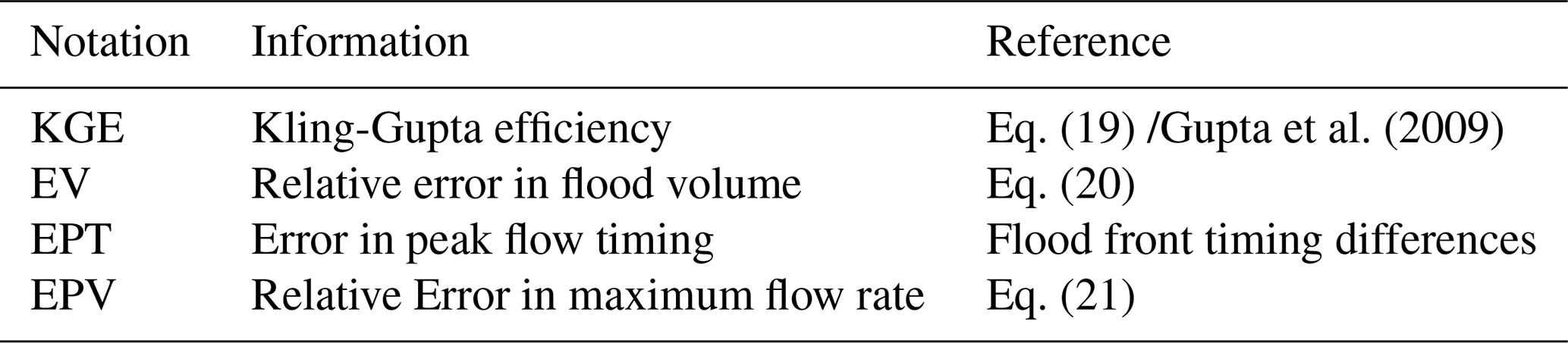
2.3.10 Hydrological Skill Metrics

The Kling-Gupta Efficiency (KGE) is calculated using observed and simulated streamflow statistics at observation resolution τ (here 15 min) in this work:

$$\begin{array}{}\text{(19)}& {\mathrm{KGE}}_{\mathit{\tau }}=\mathrm{1}-\sqrt{(r-\mathrm{1}{)}^{\mathrm{2}}+{\left({\displaystyle \frac{{\mathit{\sigma }}_{\mathrm{sim}}}{{\mathit{\sigma }}_{\mathrm{obs}}}}-\mathrm{1}\right)}^{\mathrm{2}}+{\left({\displaystyle \frac{{\mathit{\mu }}_{\mathrm{sim}}}{{\mathit{\mu }}_{\mathrm{obs}}}}-\mathrm{1}\right)}^{\mathrm{2}}}\end{array}$$

where r is the correlation between simulations and observations, σ_obs is the standard deviation of observed discharge, σ_sim is the simulated discharge standard deviation, μ_sim and μ_obs represent the average simulated and observed streamflow values, respectively.

The relative volume error (EV) is the relative difference between simulated flood volume and observed flood volume:

$$\begin{array}{}\text{(20)}& \mathrm{EV}={\displaystyle \frac{V_{\mathrm{sim}}-V_{\mathrm{obs}}}{V_{\mathrm{obs}}}},\end{array}$$

where V stands for volume of the flood. An EV > 0, and an EV < 0 mean overestimation and underestimation, respectively.

EPT refers to the error in peak flow timing between observations and simulations. For its calculation, only the highest peak is selected for calculating EPT if more than one peak is present. In this work, EPT is determined by considering the entire flood rising limb to account for the steepness of the rising limb, specifically, both the flood starting timing and the maximum flood timing from the flood front rising limb are used for calculating the EPT.

EPV or error in peak volume (Q_max, m³ s⁻¹) is a relative error calculated using peak flows from observations and simulations, and the equation is below:

$$\begin{array}{}\text{(21)}& \mathrm{EPV}={\displaystyle \frac{Q_{{max}_{\mathrm{sim}}}-Q_{{\max }_{\mathrm{obs}}}}{Q_{{\max }_{\mathrm{obs}}}}}\end{array}$$

2.3.11 Study Domain and Model Setup

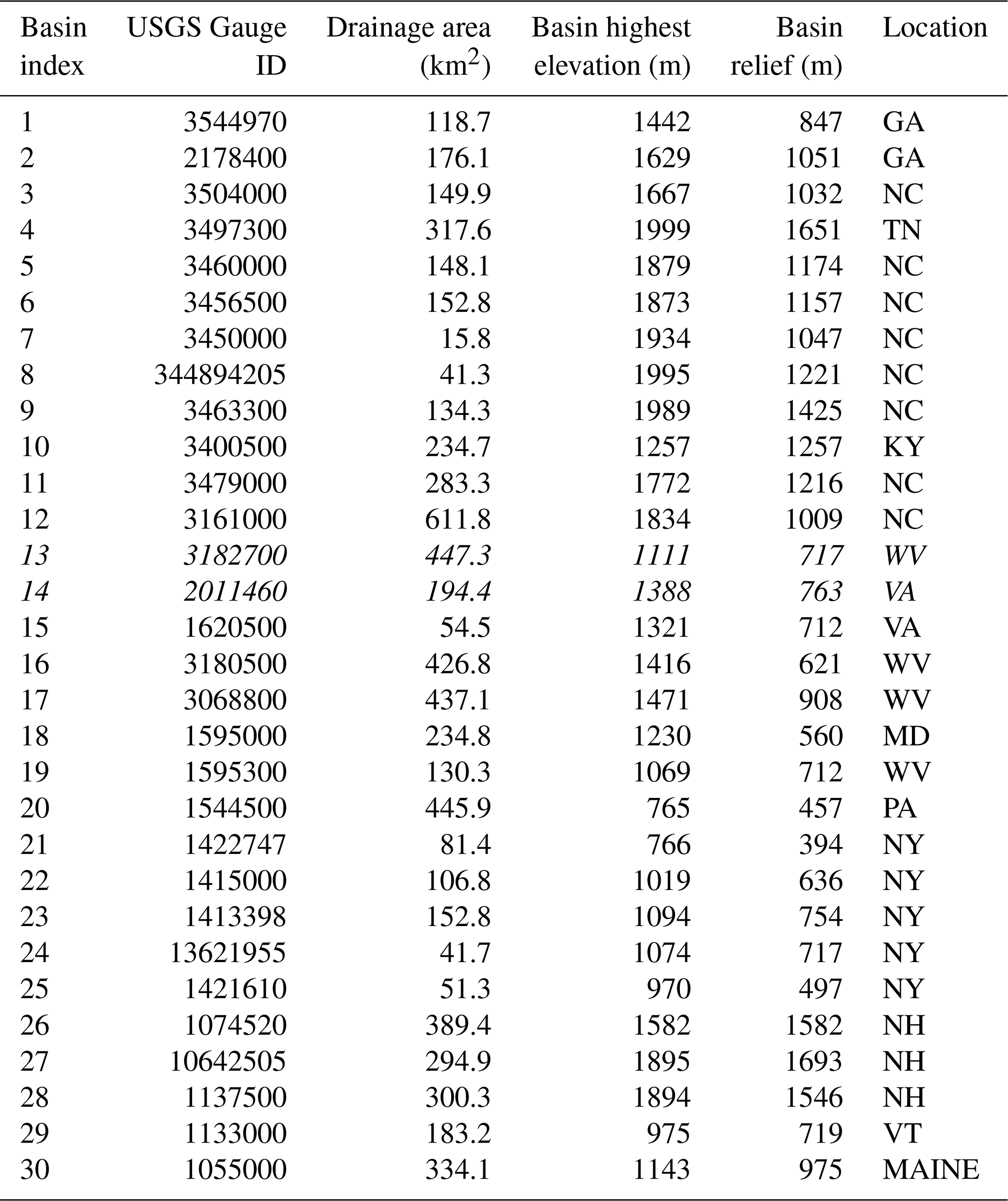
An initial 30 gauged headwater basins with areas and quality streamflow records were identified from south to north along the Appalachian Mountains (Fig. 4, Table 3). Basin01 and Basin30 are over 2000 km apart, with diverse weather and climate regimes, and large differences in geomorphology and hydrogeology. The smallest basin (Basin 07) and the largest basin (Basin 12) were discarded because their areas were less than 20 km² and greater than 600 km², respectively due to being too small for IRC at 250 m resolution and too large for IRC due to complex hydrologic response from different catchments not all impacted by the same rainfall event. Note that an additional 2 basins (Basin 13 and 14) were later discarded from inclusion in the final data set as explained in Sect. 3.2 and 3.2.1. Therefore the final published StageIV-IRC product includes 215 events in 26 basins.

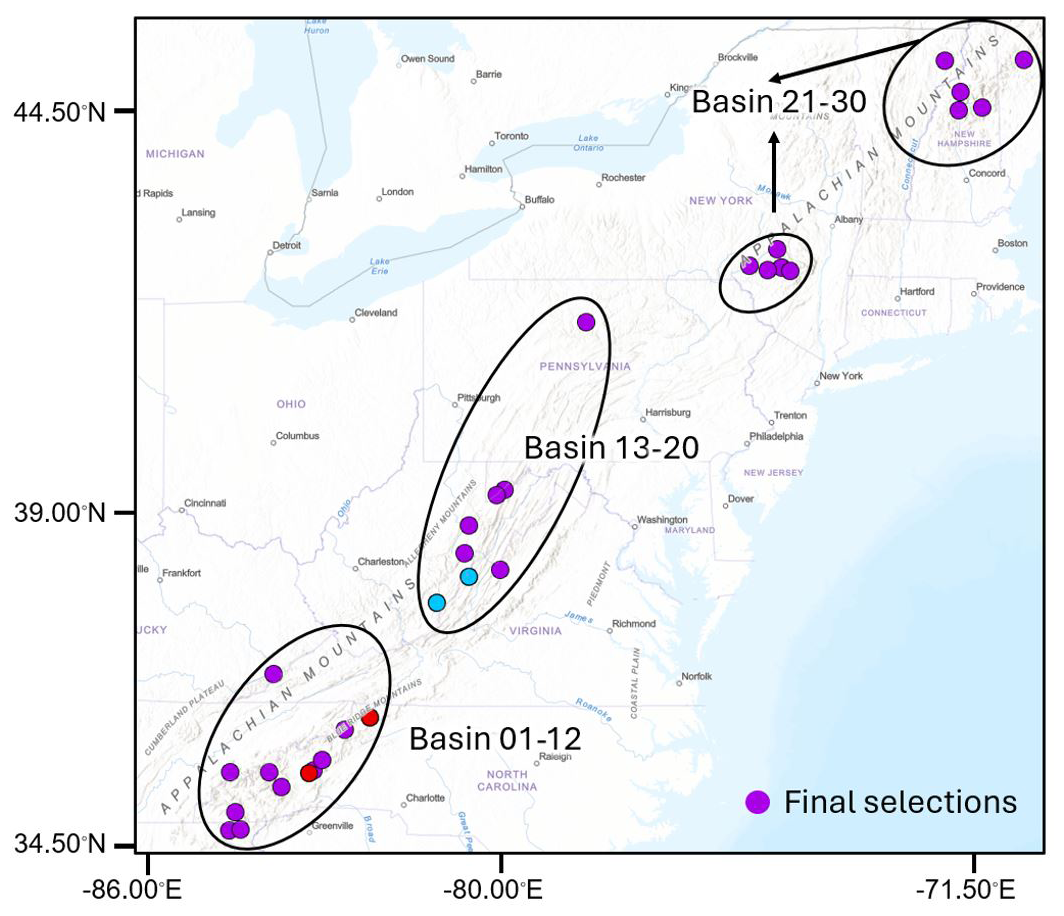
Figure 4 Map of the Continental United States (CONUS) and headwater basins studied in this work. Basin information is available in Table 3. Sub-regions are delineated as the following for discussion purposes only: Northern, Central and Southern Appalachian Mountains (NAM, Basin 21-30; CAM, Basin 13-20; SAM, Basin 01-11). Basins 07 and 12, marked with red symbols, were discarded due to basin size criteria. Basins 13 and 14 with blue symbols were discarded due to the importance of karst hydrology processes that are not represented in the hydrology model used to conduct the IRC. This figure is adapted from Liao and Barros (2025b).

Table 3 Information table for selected basins and corresponding streamflow gauges used in this work. This table is adapted from Liao and Barros (2025b). Basin 07 and Basin 12 are the smallest and largest basins respectively and were removed from further analysis. Basin 13 and 14 (Italic font) represent basins located in Karst terrain, which are not included in the final published data due to the lack of Karst hydrology processes in the hydrology model and consequently lesser performance of the IRC.

Soil-related parameters were downloaded from a global high-resolution (1 km) soil data repository (Zhang et al., 2018). For each basin, the vertical hydraulic conductivity remains the same for the entire soil column. The lateral hydraulic conductivity in the unsaturated zone was assumed to be two to three orders of magnitude larger than the vertical conductivity in the shallow soil layers, with higher values where the stone fraction in the soils is higher (Carlson, 2010; Freeze and Cherry, 1979). The final scaling factors were obtained through simple sensitivity analysis to match the curvature and slope of the observed subsurface runoff recession curves (e.g., Linsley et al., 1982; Chen and Kumar, 2001; Yildiz and Barros, 2007), and scaling factors are finally determined as: 1500, 150, 15 and 1.5 for layer 1 (0–10 cm below terrain surface), layer 2 (10–75 cm below terrain surface), layer 3 (75–200 cm below terrain surface) and layer 4 (2–20 m below terrain surface), respectively. No parameter optimization is done in this work, as the primary focus of this work is to develop a QPE dataset that can consistently close the water budget while controlling uncertainties from other sources, largely advancing the understanding of QPE uncertainties across climate, weather, and geomorphological regimes.

Flood-producing events were selected for headwater basins with areas ranging between 50–500 km² (Table 3) for recent years from January 2021 to April 2024. A qualified event is determined based on the observed peak flow, which must surpass 95 % of available flow measurements for each basin. The choice of 95 % is a compromise because 99 % would yield too few events, while 90 % would be too close to the annual flood. Additionally, rainfall runoff response time must be shorter than or equal to 6 h to be qualified as a flash flood event. Only warm season precipitation events from 2021 to 2024 are finally considered. Here, the warm season is specifically defined as from 1 April to 30 September. Note: data quality control is enforced, and events with missing streamflow records are discarded.

For the Cataloochee Creek Basin (Basin05), located in the SAM known to have experienced multiple flash floods in the past (Tao and Barros, 2013 and 2014), Liao and Barros (2023) created a Historical Flood Record database (HFR) that includes a large number of extreme rainfall events from 2008 to 2017. The event selection criteria when developing HFR also use the same 95 % flow threshold method. The difference is that the HFR also includes multiple winter-time liquid precipitation events that result in cold-season flash floods. In total, there are 54 warm-season events for Basin 05 in HFR, and these events are also used to expand the study sample size in this work.

To initialize the DCHM, a traditional spin-up approach is used with iterative runs for the hydrological year of 2021 (from the end of April to the end of September), and it generally reaches equilibrium after 3–5 iterations. Subsequently, DCHM is continuously running from the beginning of October 2021 onwards, to derive initial conditions for events after 30 September 2021. During this spin-up process, no parameter calibration is involved. The initial conditions are extracted from the last iteration of spin up run, and the following model outputs generated after 1 October 2021.

2.4 Caveats

In the entire study domain, rain gauges are only installed in the Southern Appalachians, specifically in the vicinity of the Cataloochee Creek Basin (Basin 05). However, the rest of the regions are not equipped by raingauge networks, and therefore, no rain gauge bias correction is done for those basins, and the downscaled original dataset StageIV (i.e., STIV_D) is used as input for the IRC method and hydrological simulations in this study.

As an important component of the IRC framework, the Lagrangian tracking algorithm is only implemented when hydrological window changes, rather than following model temporal resolution (i.e., 5 min), due to practical computational constraints. Additionally, we do not differentiate peak flow points and recession inflection points between simulations and observations when classifying hydrological flow regimes/windows, and consistently use observations delineate hydrological windows simply because (1) particle locations are inherently much more uncertain when simulation time is getting longer partially due to numerical truncation errors and grid-based abruptly-changing velocity fields used in the Lagrangian tracking algorithm, and (2) the computational costs of the tracking algorithm. Very short travel times (i.e., < 15 min) are ignored because of temporal resolution restrictions from streamflow observations. A systematic use of 24 h for event total duration is imposed in this work to reduce excessive tracking workload, which might be problematic for events with very long and heavy tails, though not common for flash flood events in headwater basins.

The IRC-ICC recursive framework allows us to quantify QPE uncertainties more realistically by improving initial soil moisture estimation, and this framework is numerically efficient in terms of reaching hydrological equilibrium state within 3–5 iterations. In this work, the stable state of IRC-ICC is reached when the KGE changes are bound by 0.05.

3 Results and Discussion

3.1 Rain gauge Bias Correction

The climatologically corrected STIV_DBKC fields have a significantly accurate diurnal cycle compared to only event-scale bias-corrected STIV_DBK. This process is illustrated in Fig. 5 for one rain gauge from each side of the ridges (eastern side: left panel; western side: right panel) in the Southern Appalachians.

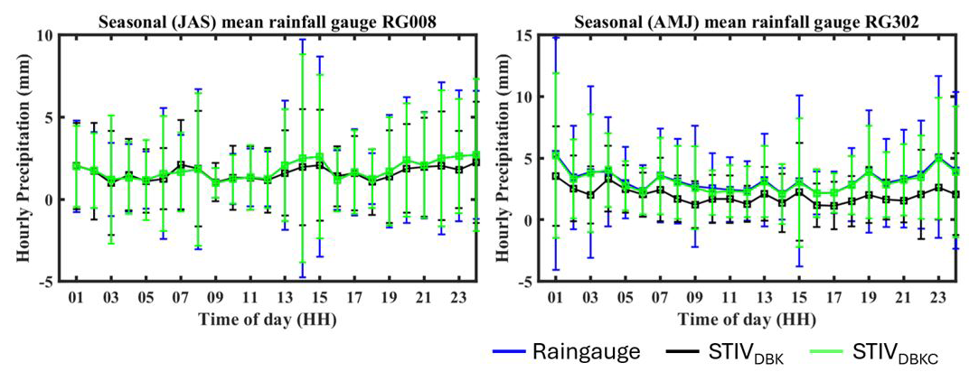
Figure 5 Examples of raingauge measurements showing the diurnal cycle of different seasons at different locations: Left panel – raingauge RG008 located in the eastern ridges for the Summer (JAS: July–August–September) season. Right panel – raingauge RG302 located in the western ridges for the Spring (AMJ; April–May–June) season. Rain gauge measurements (blue); StageIV_DBK (black); StageIV_DBKC (green). This figure is from Liao and Barros (2019).

Original StageIV_D show higher biases over the western ridges (e.g., right panel) for all hours of day, illustrating the difficulties of capturing seeder-feeder enhancement of low-level precipitation systems (Duan and Barros, 2017). Also, the mid-day dry bias has been a problem for radar measurements in this region. (e.g., Arulraj and Barros, 2019). Results show that StageIV_DBKC datasets capture precipitation climatology better with smaller missing detection errors compared to original StageIV. Figure 6 shows the diurnal characteristics of the missing percipitataion for two raingauge locations for winter season (January–February and March – JFM) using StageIV, and this phenonemon is observed for both the StageIV_D (black) and StageIV_DBK (cyan). These missing cases correspond to light rainfall that have small rainfall measurements at rain gauge locations (< 1.5 mm h⁻¹, bottom row). After applying precipitation climatology corrections, the missing issue in StageIV_DBK is significantly alleviated and much better results are shown in StageIV_DBKC fields (green).

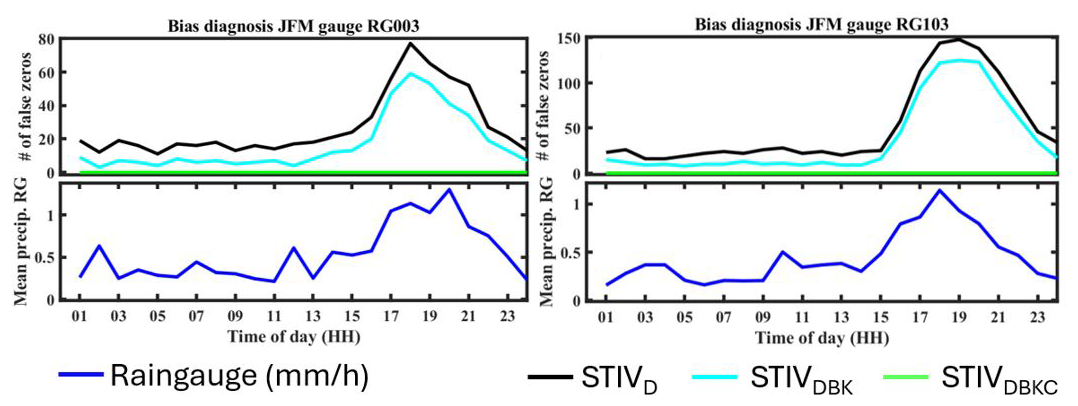
Figure 6 Top row – The diurnal cycle of missing precipitation at RG003 (Eastern ridges) and RG103 (Inner regions) for January–February–March (JFM) using various products. Bottom row – corresponding rain gauge climatology (blue). StageIV_D (black); StageIV_DBK (cyan); StageIV_DBKC (green). This figure is from Liao and Barros (2019).

The seasonal HSS, TS, and RMSE of STIV_DBKC are significantly better than those of STIV_D throughout the day using 10-year averages (Fig. 7a). It is worth noting with increasing precipitation rate threshold (Fig. 7b), threat score does not show decreasing trend, meaning raingauge bias correction for heavy rainfall events works well. Figure 7c shows RMSE performance conditional on rain rate at diurnal and seasonal scales. Overall, the RMSE is generally less than 0.1 mm h⁻¹ except in the cold-season morning and late afternoon, which can be partially attributed to snow events because these raingauges are not heated.

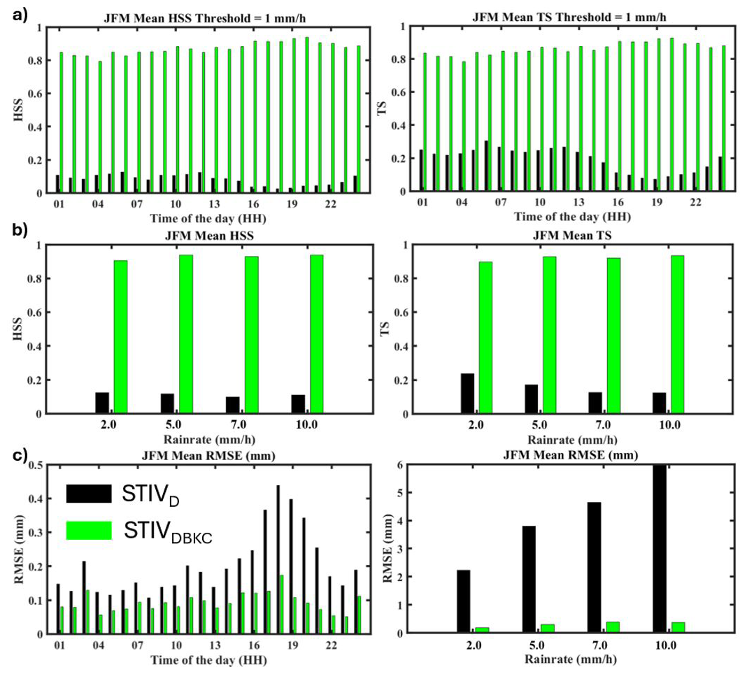
Figure 7 Statistical evaluation summary for winter precipitation (JFM, January, February, and March): (a) Diurnal cycle of mean HSS and TS statistics including all rain gauges calculated using all data from 2008 to 2017: STIV_D (black) and STIV_DBKC (green); (b) HSS and TS statistics calculated using different rain rate thresholds over the same 10-year period; (c) Diurnal cycle of rain rate RMSE at seasonal-scale, and its dependence on observed rainfall rate. This figure is from Liao and Barros (2019).

3.2 Hydrologic Correction

The coupled IRC-ICC was originally developed and applied in Basin 05, the Cataloochee Creek Basin, and an example showing the results from iterations is demonstrated in Fig. 8. The notation follows the definition in Fig. 3. Note that the STIV_DBKC data derived in Sect. 3.1 are further downscaled to 250 m and used for hydrological simulations in this section. For all other basins (except Basin05), rain gauges are not available, and STIV_D data are used instead.

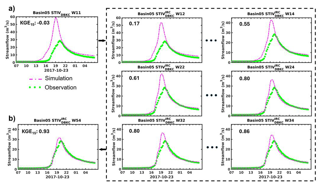
Figure 8 The IRC-ICC performance in Basin05 as an example for the 23 October 2017 event (Basin05: Cataloochee Creek Basin, NC). This event is part of the 2017 Hurricane Nate. This figure contains (a) hydrological responses when precipitation forcing is the STIV_DBKC. The dashed rectangular plot consisting of intermediate results including each iteration from the IRC-ICC framework (Fig. 3). (b) the hydrological equilibrium of the IRC-ICC after 5 iterations. This figure is adapted from Liao and Barros (2025b).

It is demonstrated that IRC-ICC produces stable results after about 3 to 4 iterations without significant oscillations for this specific extreme flood event. In general, for less significant events, IRC-ICC reaches equilibrium faster (merely three iterations), providing fast and convergent corrections. As explained earlier, the equilibrium state is reached and thus IRC-ICC is stopped when oscillations in simulated KGE are within 0.05, and then IRC-ICC is stopped immediately. This study suggests that for most events, three iterations is a good rule of thumb. The difference between the initial 4D ($x,y,z,t$) rainfall forcing and the final result of the IRC-ICC is the general IRC correction.

3.2.1 Systematic Application of IRC-ICC

The IRC-ICC is systematically executed in the 28 basins located in the Appalachians for 225 events, and examples are displayed in Fig. 9.

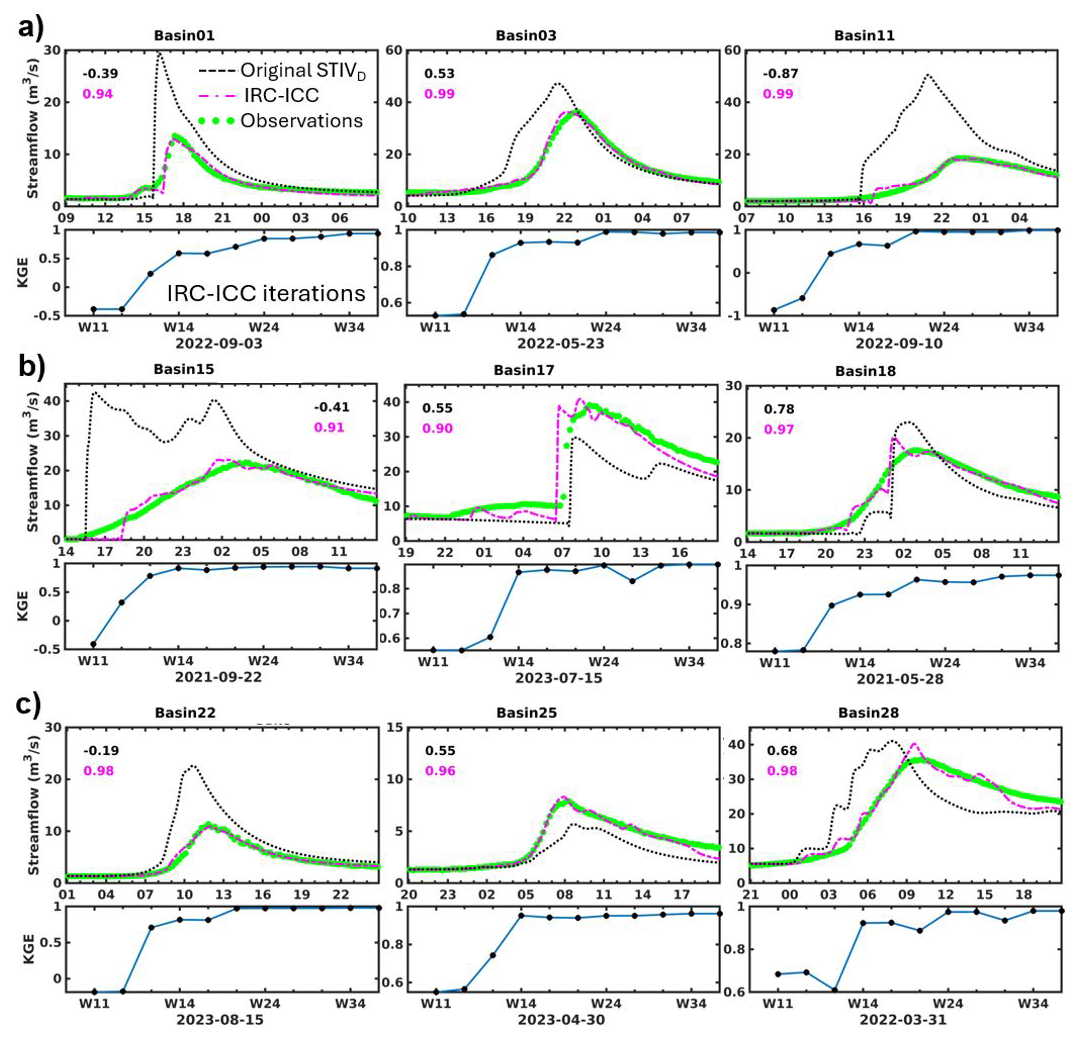
Figure 9 The IRC-ICC performance for different subregions, include (a) 3 events from the Southern Appalachians; (b) 3 events from the Central Appalachians; and (c) 3 events from the Northern Appalachians. The IRC-ICC KGE evolution plots from iterations are included below the hydrographs. The black and pink line are from the original STIV_D and the IRC-ICC equilibrium state (${\mathrm{STIV}}_{\mathrm{D}}^{\mathrm{IRC}\ast }$), respectively, and KGE values are displayed as colored numbers in the top left corners. This figure is adapted from Liao and Barros (2025b).

Simulated streamflows generally have better performances in the Northern and Southern Appalachian Mountains (NAM, SAM) compared to the Central (CAM). Specifically, in the Karst region along the interstate border of Virginia and West Virginia in the CAM, for Basins 13 and 14, where there are numerous caverns and natural tunnels facilitating fast subsurface flow response, that is, sinking and subterranean streams (https://www.dcr.virginia.gov/natural-heritage/vacavetrail and https://docslib.org/doc/2284608/west-virginia-tax-districts-containing-karst-terrain, last access: 12 March 2026). The current version of the DCHM does not have a specific module designed for karst geology and karst hydrological processes. Thus, the IRC-ICC results in these locations are impacted by model structural uncertainty. Here, the advantage of not calibrating model parameters becomes apparent. It would be possible to calibrate model parameters to improve model simulations; however, the physical basis and transferability of the IRC-ICC results would be compromised. The 10 events in Basins 13 and 14 are therefore discarded (example: Fig. A4). This point of discussion is highlighted here to reinforce the value of the data set presented in this manuscript for applications with other hydrologic models, including model calibration, where model structural uncertainty is not a primary concern at resolved scales.

Event 10 June 2021 in Basin 19 (see Fig. A4) is an example of an event with a complex hydrograph (e.g., multiple minor flood peaks around one major flood peak) that requires more hydrological windows (see Fig. 3). Subtle changes in the hydrograph shape could be indicative of spatial shifts in runoff production from one tributary to another following the track of storm cells over the basin. Indeed, depending on the weather system and regional topography, the travel velocity of such cells and their life-cycle may require finer spatial and temporal resolution both for the hydrological model and for the tracking algorithm to capture changes in the spatial structure of precipitation, especially in the case of summer thunderstorms. For the systematic production of this data set, a 5-window IRC-ICC framework was applied, including a pre-rising-point segment, rising limb, early recession, and late recession (separated by the recession inflection point).

3.2.2 IRC and IRC-ICC Precipitation Corrections

Accumulated rainfall totals per rainfall event are calculated for both the IRC-only product and post IRC-ICC products. Subsequently, these rainfall totals are directly compared against original product STIV_DBKC. Examples are shown in Fig. 10, categorized by seasons in the Cataloochee Creek Basin (Basin05). Again, the warm season is defined as 1 April to 30 September, and the remaining events are defined as the cold season, with only liquid precipitation events studied in this work.

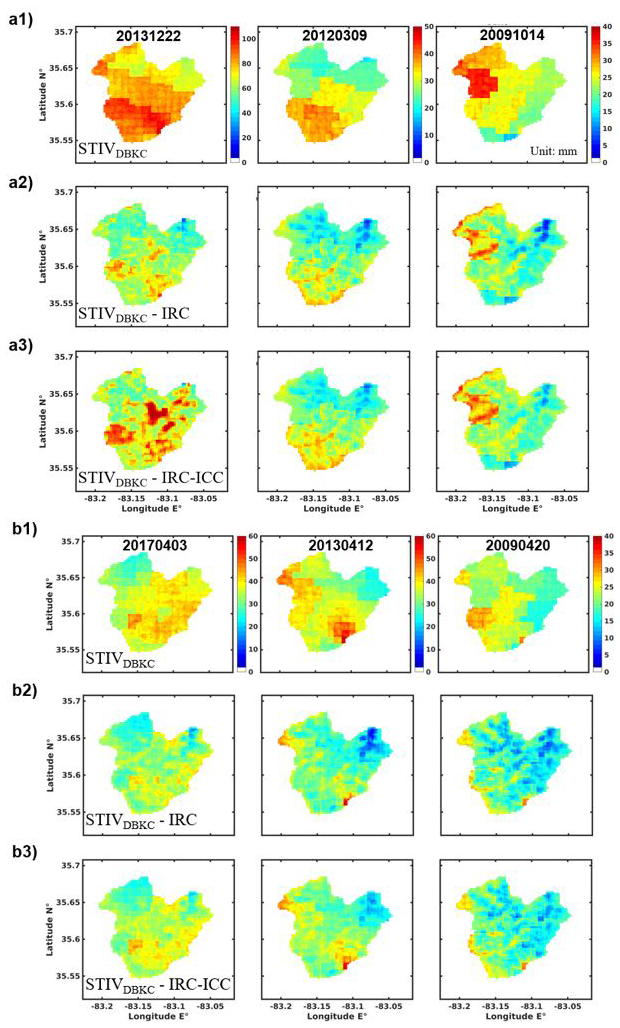
Figure 10 Event total precipitation maps for three cold season events (a) and three warm season events (b). Each column represents one event, and each row represents one precipitation product: STIV_DBKC, ${\mathrm{STIV}}_{\mathrm{DBKC}}^{\mathrm{IRC}\ast }$from IRC-only framework, and ${\mathrm{STIV}}_{\mathrm{DBKC}}^{\mathrm{IRC}\ast }$ from the coupled IRC-ICC framework. This figure is adapted from Liao and Barros (2025b).

The original QPE (a1 and b1) shows abrupt changes in rainfall intensity, which is a common issue of radar observations at high spatial resolution. On the contrary, the IRC-corrected precipitation maps demonstrate precipitation features aligning with landform, showing strong spatial precipitation gradients along ridges and adjacent valleys (examples are listed in Fig. A3). The spatial correlation between orographic precipitation and topography is observed across all mountain ranges, including the Appalachians (e.g., Konrad, 1994; Smith et al., 2011; Wolvin et al., 2024). Note the dark blue colors in Fig. 10 corresponding to very low precipitation near the basin outlet are an artifact of the IRC tied to very short travel times that cannot be fully resolved even at fine scales of 250 m and 5 min. However, these artifacts are much reduced for the IRC-ICC due to the reduction of uncertainty in initial conditions, as shown for the 14 October 2009, 20 April 2009, and 12 April 2013 events because of overall basin-wide travel time improvement. It is worth noting that these three events are relatively mild events, indicating a larger impact of IC on relatively less extreme events because of the critical role of IC in runoff generation mechanisms and travel times distributions. Thus, the extreme event precipitation product obtained from IRC-ICC is the data set recommended for applications with other hydrologic models.

3.2.3 Precipitation and Hydrologic Skill Metrics

Event-total precipitation maps are calculated for each basin and event, and basin-scale precipitation statistics (e.g., mean and standard deviation) are derived for each event-total precipitation map. These statistics are plotted in Fig. 11, and subregions are separated by vertical black lines. Basins 01 to 11 are located in the SAM, Basins 12 to 20 are located in the CAM, and Basins 21 to 30 are located in the NAM. Basins 13 and 14 are not included in the statistics.

Figure 11 Summary charts of precipitation statistics for all event-total precipitation maps. Basin precipitation average and standard deviation for each event are represented by circles and triangles in the top and bottom panel, respectively. Each panel consists of 3 sub-regions by vertical black lines: the Southern Appalachian Mountains, Central Appalachian Mountains, and Northern Appalachian Mountains. The list of events in Basin 05 (with event number ranging from 55 to 108) in the SAM is highlighted by a blue rectangle for further discussion in the text. The average values of all events for both the mean and the standard deviation are calculated and shown in the top right corner. Black color and pink color represent pre and post IRC-ICC QPE statistics, respectively.

It is clearly demonstrated that the change in the mean (i.e., basin-averaged event total QPE) is relatively small (from 36.10 to 38.07 mm) compared to the change in the standard deviation (from 6.63 to 14.08 mm) after the application of IRC-ICC. The small standard deviation of the original QPE suggests that the original QPE data are spatially tightly clustered with low variability (see Fig. 10a for boxy rainfall features), while the larger standard deviation post-IRC-ICC indicates spatial variability is enhanced, which is highlighted by the terrain-aligned precipitation features in Fig. 10c. The relatively small change in the mean indicates that the original input precipitation (i.e., StageIV_DBKC for Basin 05, and StageIV_D for the remaining basins) does not contain significant unconditional systematic biases across basins and events, which would lead to consistent positive or negative flood volume errors. As an exception, it is worth noting that the standard deviation of Basin 05 events does not change significantly after the IRC-ICC compared to other basins and events because rain gauge corrections from the IPHEx network are employed in Basin 05 but not anywhere else. It can never be overly emphasized that even after rain gauge bias correction, essentially a point-scale correction method, the resulting flood hydrograph exhibits significant water budget closure errors (see Fig. 12 for more discussion) on account of the high heterogeneous nature of QPE in complex terrain.

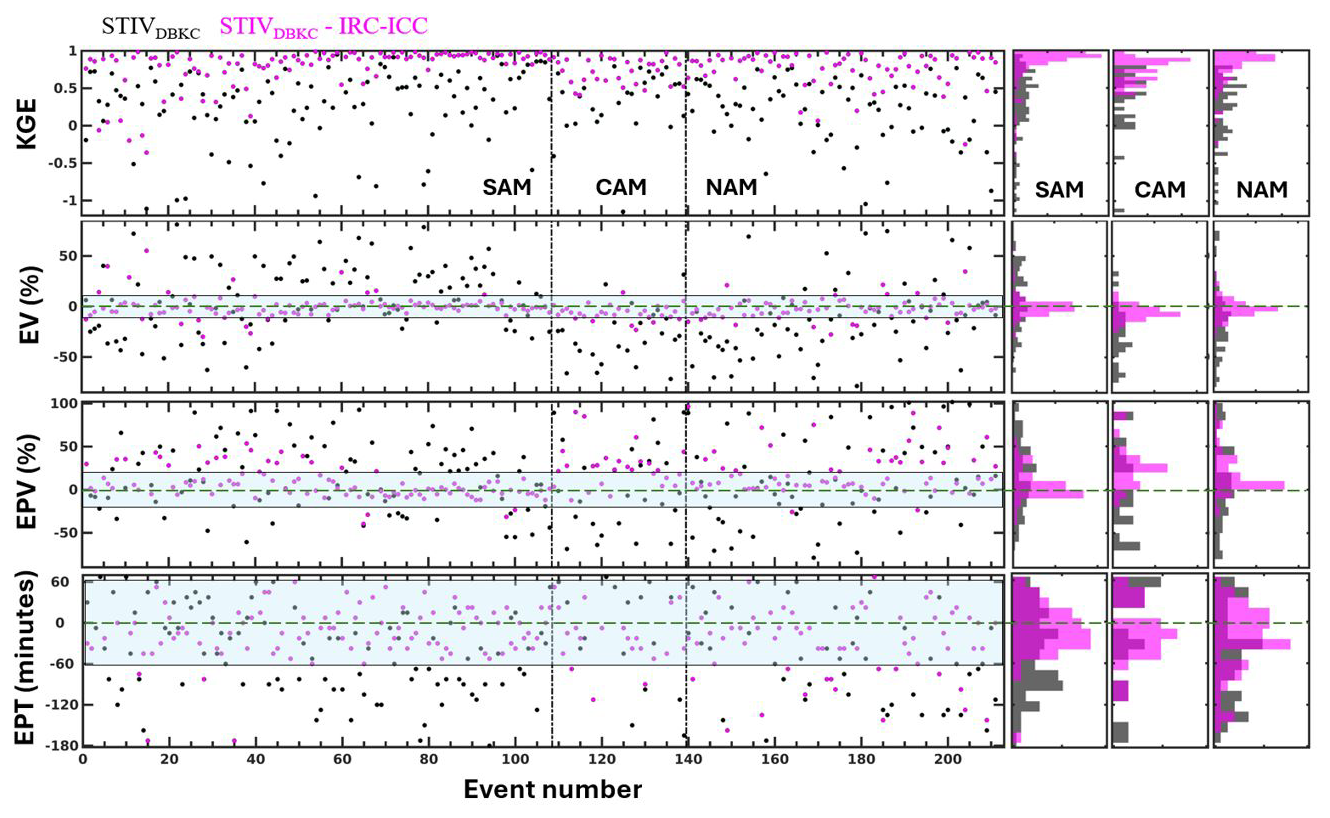
Figure 12 Summary of hydrologic skills. Green dashed lines and associated uncertainty envelopes are only for visual illustration. Hydrologic statistics are explained in Table 2. Pink and black scatters (each scatter represent one event) represent IRC-ICC, and baseline outputs, respectively. Each horizontal panel is split into 3 subsections by vertical black lines representing the 3 subregions. Histograms graphs on the right hand side are provided for a summary view. This figure is adapted from Liao and Barros (2025b).

The hydrologic statistics described in Table 1 using all studied events are plotted in Fig. 12.

Figure 12 shows that the median KGE across events is improved from 0.36, 0.39, 0.27 to 0.89, 0.74, 0.84 for SAM, CAM, and NAM, respectively. It should be pointed out that QPE changes for Basin 05 events (event numbers 55 to 108) are important for improving water budget closure, albeit small in magnitude compared to other events in other basins, as shown in Figs. 11 and 12, and yet critical to capture the complex precipitation heterogeneity in complex terrain to close the water budget. The results for Basin 05 illustrate the limitations of rain gauge-based bias corrections in complex terrain in general. The relatively small improvement shown in the CAM is partially attributed to the fact that DCHM does not have a proper representation of subterranean rivers in karst terrain, causing large baseflow errors during hydrograph recession and thus low KGE values. Nevertheless, for flash flood applications, peak flow magnitude, flood flow timing, and event flow volume are the most important forecast objectives, corresponding to the 2nd, 3rd, and 4th horizontal panels in Fig. 12. Overall, flood volume error (EV) is controlled within ±10 % for over 90 % of the studied events (the 2nd panel), with the median EV error being less than 5 % in the SAM and NAM after IRC-ICC corrections. Flood peak volume (the 3rd panel) is generally controlled within 20 %, which is very good for extreme events in regions without ground-based observations except for radars placed far away. This is demonstrated by Tropical Storm Fred on 17 August 2021: an event that caused floods in multiple SAM basins, caused five deaths, and resulted in an economic loss of more than USD 1 billion. Note the KGE for this event is improved to 0.9, and peak timing errors are < 30 min using IRC-ICC. Timing errors (shown in the 4th subplot) are bounded by ±60 min for the major of the events for post IRC-ICC datasets, though some outliers exist potentially due to complex antecedent land surface physics (e.g., rain on snow) for April events, particularly in the CAM and NAM.

Events associated with significant timing errors (more than ±90 min) are investigated in detail. These include the 8 July 2023 event (event number 185) for Basin 27, which is located in New Hampshire (the estimated flood front occurs too early by 2.5 h). This was a localized summer thunderstorm event, only taking 30 min to reach its peak flow. The fast changes in the hydrological regime require much more windows than the current classic 5-window settings used in the IRC-ICC framework. The event on 27 May 2022 (event number 118) in Basin16 located in West Virginia is characterized by a slow rising limb. Note Basin16 is partially located in a complex region with karst features (e.g., sink holes) in the Greenbrier-river valley. Finally, the event 22 September 2021, a complex rainfall system characterized by multiple rain cells passing through the Basin 19 quickly (event number 133), requiring smaller hydrological windows to capture highly variable rainfall-runoff responses than the 5-window default IRC-ICC architecture: baseflow segment, pre-rising segment, flood rising limb, early and late recession.

Overall, large improvements in QPE are achieved, resulting in hydrological improvements in aspects of peak magnitude, flood total volume and flood front timing. Due to the dependence of IRC-ICC on travel time distributions, it cannot be used when precipitation is missing or there are severe timing errors because of the lack of water travel time trajectories to distribute corrections. From a practical point of view, the QPE IRC-ICC correction is in nature a type of space-time bias correction. The improved QPE data facilitates the development of QPE error models, which is demonstrated by the same authors (e.g., Liao and Barros, 2023), providing a path towards correcting remote-sensing products to support hydrometeorological studies and advancing the calibration of hydrological models with significantly less forcing uncertainty.

3.2.4 Independent Verification

As mentioned in the introduction, precipitation measurements are limited in the Appalachians except for the IPHEx rain gauge network (Fig. 1). Currently, the NEXRAD radar network remains the widely used precipitation monitoring system in this region in spite of well-documented low radar quality coverage over radar gaps in the mountains. The Multi-Radar/Multi-Sensor (MRMS) product (Zhang et al., 2016), which is developed using NEXRAD radar measurements similar to StageIV, is created at 1km resolution and is used here for independent verification.

First, original MRMS data are downscaled to the same resolution as StageIV_D datasets (250 m, 5 min) and used as inputs for DCHM. Hydrological simulations in this section are using the same model configuration and initial model states for the purpose of a meaningful comparison, including the following datasets: MRMS_D, StageIV_D, and IRC-ICC StageIV_D as shown in Fig. 13. Figure 13a shows that MRMS and StageIV QPE have similar results. Second, the IRC-ICC StageIV_D have generally a good agreement with MRMS_D similar to StageIV_D. However, for some cases, where rainfall is dramatically underestimated by the radar system and KGE values are low, IRC-ICC is shown to provide effective corrections. Otherwise, the IRC-ICC generates physically constrained corrections spatially (see Fig. 10), achieving high KGE values for flood simulations. Figure 13b shows the histogram of the KGE values across different rainfall products for all events. Overall, simulated streamflows using MRMS_D and StageIV_D exhibit similar hydrologic performance (the median KGE across events is close to 0.20), on the contrary, post-IRC-ICC StageIV_D produce flood simulations with a median KGE above 0.80.

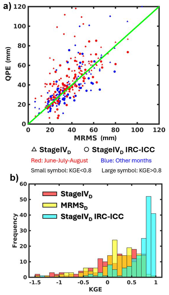
Figure 13 (a) Event total QPE plots for various QPE datasets conditional on seasons and KGE values; (b) KGE distributions across events using different QPE datasets. This figure is adapted from Liao and Barros (2025b).

4 Discussion and Future Work

Limitations in this study stem mainly from computational constraints rather than methodology. A default 24 h flood duration window is imposed, implying that for long-lasting floods, due to significant slow interflow and baseflow contributions, are not considered. The current version of the IRC-ICC framework was built to support flash flood studies and only targets shallow subsurface moisture transport, given the critical importance of shallow soil moisture on the regulation of flood generation and propagation in steep terrain. It is worth noting that for long-lasting rainfall events or regions with relatively flat terrain, slow interflows would become more important in terms of regulating flood timing, flood volume, and post IRC-ICC QPE.

While the IRC results could be further optimized if carried out at the same frequency as the model resolution, therefore eliminating any artifacts due to inadequate sampling and updating of travel time distributions, and while there is room to improve the IRC-ICC framework through improved model physics and resolution, utilizing 3D velocity fields to capture the full travel time distributions, and using different models to generate IRC ensembles. to test and calibrate hydrologic models for an intercomparison study, advancing flood forecasting skill, and to support emergency management response.

5 Data availability

The StageIV-IRC dataset at 250 m 5 min resolution for 26 basins and 215 events is available at: https://doi.org/10.5281/zenodo.14028866 (Liao and Barros, 2025c), excluding Basin 07 (the smallest basin), 12 (the largest basin), 13 (Karst terrain), and 14 (Karst terrain) based on previous discussion. Associated geographic documentation of the selected basins is also provided via the same link. Initial soil moisture distributions for the studied events are also available in the same Zenodo repository.

The StageIV-IRC precipitation data consist of precipitation fields at 250 m every 5 min for each event and headwater basin. The StageIV radar product was first downscaled from 4 km to 250 m using fractal downscaling, resulting in STIV_D. Hourly data were linearly interpolated to 5 min. The IRC-ICC framework was applied to STIV_D to derive the StageIV-IRC product that is made public for all events across all basins except for Basin 05. Because high quality data are available from rain gauge network in Basin 05 since 2007, a series of precipitation corrections based on these data was applied to the STIV_D data including event-scale bias correction, decadal-scale bias correction, and ordinary kriging. The resulting data is STIV_DBKC. For Basin 05, the IRC-ICC framework was applied to STIV_DBKC.

This work relies on an uncalibrated distributed hydrologic model to simulate rainfall-runoff response. Model parameters are obtained from the literature and from publicly available datasets. The key assumption in this work is that precipitation uncertainty of extreme events dominates over other hydrologic uncertainty tied to model structure and model parameters. Consequently, differences between simulated and observed hydrographs at stream gauge locations are attributed to precipitation errors upstream in the contributing watershed.

This work is expected to work the best for heavy precipitation events that are typically associated with large precipitation measurement and estimation uncertainties. It is recommended that readers should address uncertainties in precipitation estimation at watershed scale before parameter calibration in hydrologic modeling studies.

6 Conclusions

QPE has been an enduring challenge in hydrology, particularly in complex terrain. Ground-based radar QPE is plagued with uncertainties from multiple sources, while rain gauge networks are scarce and suffer from the lack of representativeness in the mountains. To address this grand challenge, we develop a series of corrections from point-scale to watershed-scale encompassing event bias, climatology, and water budget closure: the IRC-ICC framework. To our knowledge, this is the first QPE dataset that meets standard statistical evaluations against point-based measurements where available and meets water budget closure at flood-event scale, consistent with nonlinear rainfall-runoff processes in headwater basins, and achieves superior hydrological performance at sub-hourly.

The IRC-ICC framework is successfully adopted in 26 mountainous basins (excluding the basins that are heavily overlapped with Karst terrain) in the Appalachians for 215 events with robust success, yielding substantial improvements of streamflow simulation, particularly in terms of flood volume and timing. The tracking algorithm in the IRC-ICC framework is only updated when shifting from one hydrological window to another, but not every time step. With enough computational resources, post-IRC-ICC QPE data should further improve by capturing transient travel time distributions between model time steps.

When using the StageIV-IRC product, flood timing errors are controlled with one hour for 90 % of events, compared to less than 20 % when using original StageIV, while the median KGE improved from 0.34 to 0.86 across the events. This change in KGE is achieved by significant changes in the space-time variance of precipitation that in turn impacts the space-time variability of rainfall-runoff processes. Results illustrate the importance of initial conditions for less severe rainfall events, particularly during the beginning of the event, which influences subsequent streamflow simulations. It should be emphasized that physical parameters are not calibrated for any precipitation event in any basin in this work. This physics-based IRC-ICC framework can capture the fundamental physics involved in flash flood events: essentially the fast rainfall-runoff responses in surface and shallow subsurface layers; therefore, skillful hydrologic prediction is achieved without model calibration. Instead, the focus is on getting the forcing right.

The IRC-ICC is a general framework that can be incorporated into any distributed hydrological model. Thus, the StageIV-IRC dataset also enables meaningful intercomparison among different radar QPE datasets, providing physics insights into QPE error structure from a water budget closure perspective, toward improving radar retrievals and to characterize radar-specific errors related to radar operations at high spatial resolution in the mountains. The demonstrated success of StageIV-IRC in ungauged basins strongly supports the use of IRC-ICC in mountainous regions worldwide, where rain gauges are generally not available. Further, this dataset can be utilized as a reference for building machine learning models (or even deep-learning models when the number of studied precipitation events is expanded) that can learn the QPE uncertainties conditional on time of day, weather, climate and geomorphological regimes for both radar QPE analysis and forecasts, advancing the understanding and quantification of orographic precipitation uncertainty at high resolution across global mountains.

Appendix A

The detailed distribution process of water difference (wd) is illustrated in Fig. A2 following Sect. 2.3.8.

A zoom in map of the Southern Appalachians is plotted associated with DEM maps of other basins. A complete set of maps for each individual basin can be requested. Note, the rain gauges used in this study are plotted in Fig. 1, and they are primarily near Basin05.

Figure A1 Spatial rainfall fields on 15 May 2014, 06:00–07:00 UTC. Rain rates between 0 to 1 mm h⁻¹ are mapped in white.

Figure A2 Schematic depiction of the IRC framework and key mathematical equations. Panel (a) illustrates the nonlinear relationship between streamflow and precipitation, where wd represents the residual between discharge simulations and observations at the basin outlet. The variation of precipitation in the basin as a function of time is shown by the basin hyetograph in blue. The hyetograph time series (blue) spans the duration of the precipitation event between t₁ to t_n. In gray is the hyetograph over the area of interest for panels (b) and (c). To map the streamlines, water particles are launched every time step and their trajectory to the outlet is tracked and saved. Panel (b) shows the source areas of water particles launched at various time steps ($t_{\mathrm{1}},t_{\mathrm{2}},\mathrm{\dots }{t}_{\mathrm{6}}\mathrm{\dots }$) from all locations where runoff is produced, and the particles are tracked until they eventually reach the basin outlet. The streamlines of particles that reach the outlet at the same time are used to distribute the residuals backwards to the runoff source areas where the particles were originally launched (e.g., the three particles  t₃₁, t₃₂, and t₃₃ that reach the basin outlet at time t₃). Panel (c) shows the algorithm to calculate the rainfall bias correction at location t₃₁ due to the residual wd₃ at time t₃. P_i is basin averaged rainfall at time t_i, and wd₃ is the runoff volume to be corrected at time step t₃. ΔP₃₁ is the precipitation correction for pixel t₃₁, and precipitation amount at pixel t₃₁ before and after IRC are denoted by P₃₁ and $P_{\mathrm{31}}^{\mathrm{new}}$. This figure is adapted from Liao and Barros (2025b).

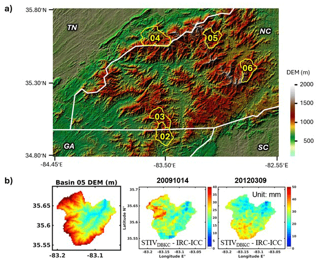
Figure A3 A zoom-in map of the Fig. 4 for watersheds in the Southern Appalachians (a). The DEM map and examples of rainfall event accumulation of Basin 05 (b) to show rainfall alignment with topography.

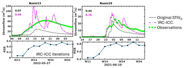
Figure A4 Examples of the coupled IRC-ICC framework application in Basin 13 and Basin 19 for discussion in the manuscript. KGE values are displayed in the top left corners. Basin 13 is located in Karst terrain, while the event in Basin 19 is an example with a complex hydrograph.