A new magnetic anomaly map for Greenland based on a combination of equivalent source modeling and spherical harmonic expansion

The Greenland Magnetic Map (GREENMAG) is a new compilation of magnetic anomaly data that covers the inland ice, ice-free coastal areas, and adjacent shelf regions of Greenland (https://doi.org/10.22008/FK2/LQN5YJ, Heincke and Szwillus, 2025). GREENMAG is based on all accessible modern regional aeromagnetic surveys from Greenland and vintage datasets without GPS positioning in areas where modern data are lacking.

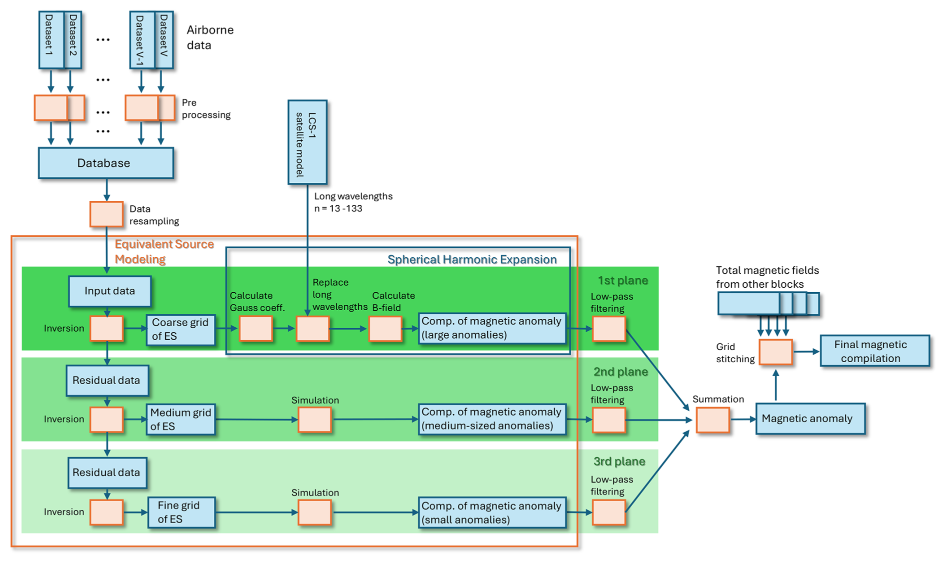
The magnetic anomaly map is generated by a combination of equivalent source (ES) modeling and spherical harmonic expansion. Hereby, the data points are used at their actual measurement location as input data for the inversion of the ES modeling. The equivalent sources are represented by magnetic dipoles that are arranged in three uniform grids with different source spacing and depths (coarsest spacing: 10 × 10 km; medium spacing: 2 × 2 km; finest spacing: 0.7 × 0.7 km). Regularization in the inversion for the different equivalent source grids are chosen such that the resulting resolution is adapted to the largely varying magnetic data coverage in Greenland. Since long wavelength components in aeromagnetic data are considered unreliable, they are replaced by the LCS-1 satellite model based on magnetic gradient measurements of the Swarm and CHAMP missions. For merging, the responses from the individual equivalent dipole sources are transferred to spherical harmonics and replaced for degree n= 13–133 by the Gaussian coefficients of the LCS-1 model.

The final magnetic anomaly map is calculated from the combined model at a constant height of 2000 m a.s.l. (WGS84) and with a grid spacing of 400 × 400 m.

The comparison between the GREENMAG and the earlier compilation from the Circum-Arctic Mapping Project (CAMP-M) highlights the enhanced level of detail now available across many regions of Greenland.

1 Introduction

The remote, Arctic, and often alpine conditions of Greenland make geophysical surveying on a regional scale generally very expensive. To systematically map large areas under such conditions, airborne magnetic mapping is considered as the cheapest and one of the best-suited methods (Golynsky et al., 2018) for gaining insight into the crustal geology of Greenland. Since areas insufficiently covered by airborne magnetic surveys can, moreover, be supplemented with lower-resolution satellite data, regional-to-continental-scale magnetic maps belong to the most uniform and consistent presentations of geophysical data in this region (e.g., Verhoef et al., 1996; Gaina et al., 2011).

In particular, for the inland ice sheet that is inaccessible for direct geological mapping and where geophysical surveying is challenging, magnetic data are often treated as the main source for extracting geological information (for example, to trace geological units under the inland ice (MacGregor et al., 2024), to build up lithospheric models (Wansing et al., 2024), to understand the heat flow patterns (Kolster et al., 2023) or to map the path of the Iceland mantle plume Martos et al., 2018). But also for the ice-free coastal areas and adjacent shelf-regions, aeromagnetic maps are considered as highly relevant to understand the geologic history of e.g., Precambrian and Caledonian orogenies (Steenfelt et al., 2021; Drenth et al., 2023), magmatic provinces and basins (Berger and Jokat, 2008), the Cenozoic and Mesozoic continental break-ups and the opening of the Northern Atlantic, Baffin Bay and Arctic Ocean (Døssing et al., 2013; Geissler et al., 2017), and are used for both mineral (Møller Nielsen, 2004; Brethes et al., 2018) and hydrocarbon (Christiansen, 2021) exploration. Depending on the application, either characterization of regional-scale deep crustal structures and features associated with magnetic long wavelength anomalies or detailed small-scaled anomaly patterns associated with e.g., dyke swarms, local faults, thrusts, and intrusions are of particular interest (Møller Nielsen, 2004; Brethes et al., 2018); and for some applications, as e.g., mineral prospectivity mapping (Heincke and Møller Stensgaard, 2017), magnetic features in various scales are important. This means that magnetic compilations suitable for a wide range of applications, and thus a broader community, should accurately both represent the long-wavelength signal and resolve detailed anomaly features.

Over the past decades, a number of Arctic magnetic anomaly compilations have been released that cover whole or large parts of Greenland as e.g., the GAMMA-5 compilation (Verhoef et al., 1996), the compilation from the Circum-Arctic Mapping Project (CAMP-M;  Gaina et al., 2011) and the compilation from the NAGTEC atlas (Nasuti and Olesen, 2014). In addition, global magnetic anomaly maps such as EMAG2V3 (Meyer et al., 2017) and WDMAM (Lesur et al., 2016) also cover Greenland. However, these global datasets typically incorporate regional sources like GAMMA-5 and CAMP-M to enhance Arctic coverage and, hence, result in similar resolution and appearance over Greenland.

In all of these compilations, fully processed magnetic anomaly grids from individual airborne surveys were stitched together to assemble large-scale compilations. Since long wavelength trends from aeromagnetic surveys are often considered unreliable, long wavelengths components in the more recent CAMP-M and NAGTEC compilations are replaced with those from satellite models. Hereby, they used wavenumber filtering techniques based on the Fourier transform to integrate the satellite models. The final compilations are presented as grids with fixed spacing ranging from 2×2 km (CAMP-M and NAGTEC compilation) to 5×5 km (GAMMA-5 compilation).

(1) Since these conventional approaches have several weaknesses (see below) and (2) since both a considerable amount of new aeromagnetic data sets and a new lithosphere model from modern satellite instruments (LCS-1 model; Olsen et al., 2017) have become available after these compilations were published, we decided to build a new magnetic anomaly compilation named Greenland magnetic map (GREENMAG). This compilation is based on a more advanced methodology and incorporates all modern regional aeromagnetic datasets from Greenland and the adjacent offshore regions that are accessible today. Our method combines equivalent source (ES) modeling (e.g., Dampney, 1969; Li and Oldenburg, 2010) and a spherical harmonic (SH) expansion (e.g., Blakely, 1995) that does not integrate preprocessed grids from individual surveys, but uses the actual line data at their original measuring locations. In the equivalent source modeling, magnetic dipoles were used as sources (e.g., Ravat et al., 2002; Dilixiati et al., 2022) that were arranged in three grid layers at different depth levels and with different lateral dipole spacing. The equivalent sources of each layer were determined in smoothing regularized least mean square inversion problem. Due to the significant number of both input data (>130 M data points) and model parameters (up to 7 M ES), an adequate data reduction strategy was required and sparse matrix solvers were used to keep the calculation manageable on a high-performance personal computer in terms of both memory and speed. In addition, we reduced the required memory by dividing the entire area into a number of overlapping blocks and performing the procedure independently for each block. At the end, the resulting magnetic anomaly maps from the individual blocks were merged to create the final magnetic compilation. For the SH expansion, the approach from Dilixiati et al. (2022) was used, which allows us to determine the Gauss coefficients directly from the equivalent sources.

This approach has several advantages compared to the conventional strategy:

1. By using data at their measurement locations, it is easier with ES modeling than with conventional approaches to consistently combine data sets from surveys that are largely overlapping and have very different acquisition parameters. For example, it is generally unproblematic to integrate a large-scale survey with a very wide line spacing of tens of kilometers and a local high-resolution survey with dense line spacing. Preprocessed grids are more challenging to stitch together because of the variations in their resolutions and appearance.

2. By using an inversion setup, (a) the different data quality of individual surveys can be taken into account by reducing the influence of less reliable data through the assignment of larger error margins during the inversion process, (b) erroneous data points can be identified by their poor data fit, and (c) systematic errors (e.g., artificial quasi-uniform shifts of data sets) can be corrected automatically.

3. The use of multiple grid levels with different dipole spacings in the ES modeling allows the strength of regularization to be adjusted separately for different wavelengths. This gives flexibility in presenting anomalies everywhere in an appropriate amount of detail and resolution. This is particularly important for this compilation due to the highly variable magnetic data density in Greenland.

4. The influence of different flight altitudes of the surveys on the magnetic responses is inherently corrected in the ES modeling and does not lead to inconsistencies when the datasets are merged.

5. The resulting ES model can be used to simulate the magnetic anomaly for any location and elevation. This allows, for example, the determination of the residual magnetic anomaly at a constant elevation.

6. Since the spherical shape of the earth is taken into account both in the ES modeling and the SH expansion, no distortions are incorporated for long wavelengths related to a flat-earth assumption.

Despite the many advantages of this approach, determining suitable inversion parameters (e.g., regularization strengths) and accurate data error estimates for all datasets requires considerable effort. As a result, multiple test runs may be necessary before achieving a satisfactory anomaly map.

The higher resolution of this new magnetic map across many regions enables direct correlation of local features – such as intrusions, dykes, and secondary faults – with regional-scale and deep-seated structures, which was not possible with previous, coarser maps. This advancement will allow for more refined and consistent interpretations of geological and tectonic processes, which are crucial for a wide range of applications such as, for example, to improve mineral prospectivity maps or to better understand processes at the continental margins.

In this contribution, we first give an overview of the airborne geophysical datasets and the LCS-1 satellite model used in the compilation (Sect. 2). We then present the methodology (Sect. 3) starting with a brief introduction of the magnetic field of a magnetic dipole followed by a description of the implementation of the equivalent source model. Next, we describe how the magnetic field on a constant height level was simulated from the equivalent source model, how the magnetic fields from the ES were expressed in spherical harmonics, and how the long-wavelength components of the satellite data were added. In Sect. 4, we summarize the preparation of the aeromagnetic data to be used as input data for the ES modeling and explain our choices of parameter settings used in the ES modeling. Finally, we present the new Greenland magnetic anomaly compilation in Sect. 5 and make a general evaluation of the quality of the compilation. In this context, we indicate exemplary a number of features that are not or little resolved in the former CAMP-M compilation, but can be clearly observed in our new compilation.

2 Aeromagnetic datasets and satellite models

2.1 Aeromagnetic datasets

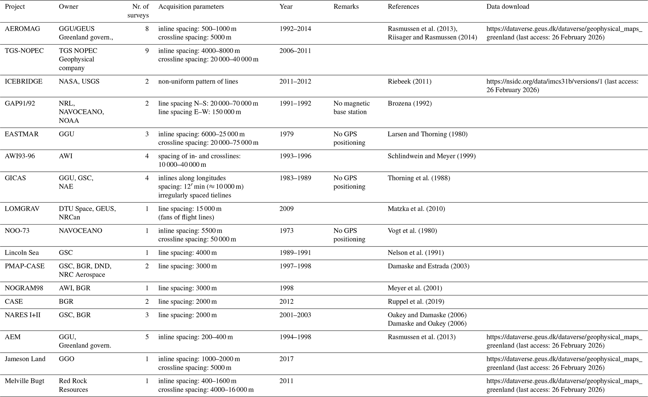
In total 50 aeromagnetic datasets were used in the GREENMAG compilation having ≈1.83 M line kilometers (Fig. 1 and Table 1). Most of them are modern regional surveys from the last three decades with high quality data and uniform data coverage; but in areas where such data are lacking, we filled gaps with older data without GPS positioning (GICAS, EASTMAR, NOO-73) and datasets with sparse survey lines (GAP91/92, ICEBRIDGE).

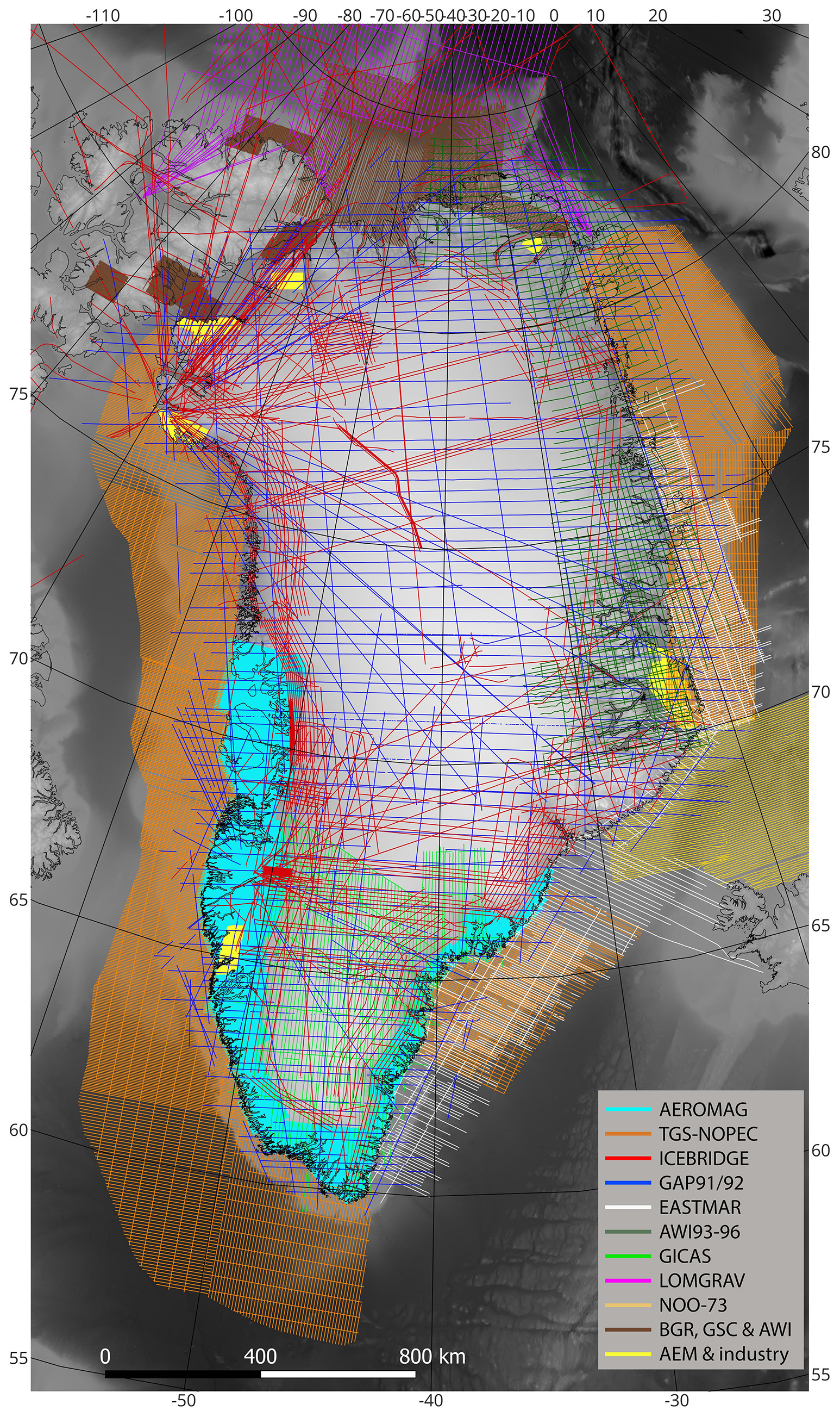
Figure 1 Line data that are used for the magnetic anomaly compilation. The different projects are distinguished by their color-coding. The topography of the GEBCO bathymetry model (https://www.gebco.net/, last access: 5 March 2026) is shown in the background.

Rasmussen et al. (2013)Riisager and Rasmussen (2014)Riebeek (2011)Brozena (1992)Larsen and Thorning (1980)Schlindwein and Meyer (1999)Thorning et al. (1988)Matzka et al. (2010)Vogt et al. (1980)Nelson et al. (1991)Damaske and Estrada (2003)Meyer et al. (2001)Ruppel et al. (2019)Oakey and Damaske (2006)Damaske and Oakey (2006)Rasmussen et al. (2013)

Table 1 Overview of the aeromagnetic datasets used in the new magnetic anomaly compilation. (Abbreviations: AWI: Alfred Wegener Institute, BGR: German Federal Institute for Geosciences and Natural Resources, DND: Department of National Defence Canada, DTU: Technical University of Denmark, GEUS: Geological Survey of Denmark and Greenland, GGO: Greenland Gas and Oil, GGU: Geological Survey of Greenland, GSC: Geological Survey of Canada, NAE: National Aeronautical Establishment, NAVOCEANO: Naval Oceanographic Office, NASA: National Aeronautics and Space Administration, NRC Aerospace: Institute for Aerospace Research, NRCan: Natural Resources Canada, NRL: Naval Research Laboratory, NOAA: National Oceanic and Atmospheric Administration, USGS: U.S. Geological Survey)

Both the coverage with regional magnetic data and the quality of the available magnetic datasets vary significantly in Greenland and the adjacent offshore regions (see Fig. 1). The coastal ice-free onshore areas of West, South and Southeast Greenland are well-covered with high-quality data from the AEROMAG surveys (collected from 1992–2013) having dense inline spacing ranging from 500 to 1000 m (Rasmussen et al., 2013; Riisager and Rasmussen, 2014), and also most of the near-coastal sedimentary basins of West, East and South Greenland were systematically surveyed with modern aeromagnetic data (inline spacing: 4 to 8 km) by the company TGS-NOPEC from 2007 to 2011. The remaining parts of the shelf regions of East Greenland are filled with vintage data from the EASTMAR project from 1979 (Larsen and Thorning, 1980) and a dataset (NOO-73) from the Naval Oceanographic Office from 1973 (Vogt et al., 1980). These datasets provide relatively dense data coverage, but suffer from poor positioning due to the lack of GPS and poor representation of long-wavelength trends (dataset EASTMAR1). Most of the offshore region north of Greenland are uniformly covered with data from several surveys (LOMGRAV, Lincoln Sea, PMAP-CASE, NOGRAM, CASE, NARES) acquired by the Geological Survey of Canada (GSC), the German Federal Institute for Geosciences and Natural Resources (BGR), the Alfred Wegener Institute (AWI) and the Technical University of Denmark (DTU); but in most parts of the ice-free costal areas of North Greenland systematic regional surveys are missing, and only a smaller portion is covered here with local AEM surveys.

Over the inland ice, dense coverage with (modern) aeromagnetic surveys is lacking. In the central and northern part, the very coarse pattern of mainly east-west-oriented profiles of the GAP91/92 project (line spacing of 20–70 km; Brozena, 1992) and the irregularly acquired line patterns from the ICEBRIDGE project provide the only aeromagnetic data in most of the area. Only in the northeast are additional data from the AWI 93/96 surveys available. In the southern part of the inland ice, the coverage is generally slightly higher since these data are complemented with the systematically flown surveys from the GICAS project (line spacing: ≈10 km;  Thorning et al., 1988). However, the GICAS datasets were collected in the 1980s without GPS positioning, and these data suffer from rather poor data quality.

2.2 Satellite model

A lithospheric magnetic field model derived from CHAMP and Swarm satellite data (LCS-1; see Olsen et al., 2017) (data download at https://www.spacecenter.dk/files/magnetic-models/LCS-1/, last access: 26 February 2026) was used for the long wavelength part of our compilation. The CHAMP and the Swarm missions were launched by NASA and ESA in 2000 and 2013, respectively. The CHAMP satellite had an orbit at altitudes lower than 350 km, but the Swarm mission consists of three identical satellites with orbits at 450 and 530 km altitudes. Unlike previous magnetic satellite models, not the magnetic fields, but their gradients, were used to build the LCS-1 model. Since gradients are less affected by large-scale external field contributions, this model is considered more robust against noise from geomagnetic activities common at polar regions. Referring to Olsen et al. (2017), the model agrees very well with other satellite-derived lithospheric field models at low degrees (degree correlation above 0.8 for degrees n≤133).

3 Methodology

3.1 Equivalent source dipole model

Equivalent source models result in a linear inverse problem, where a vector of magnetic field observations $[d_{\mathrm{1}},\mathrm{\dots },d_M{]}^T=\mathit{d}$ is used to determine a vector of the unknown source strengths $[m_{\mathrm{1}},\mathrm{\dots },m_N{]}^T=\mathit{m}$. They are linked with each other by a kernel matrix A:

$$\begin{array}{}\text{(1)}& \mathbf{A}\mathit{m}\approx \mathit{d},\end{array}$$

where an entry A_mn of A gives the effect of an equivalent source n on station m. How precisely the entries of A are calculated depends on the chosen type of equivalent source, and analytical solutions exist for “primitive” sources such as magnetic monopoles and dipoles.

For this compilation, dipoles are selected as equivalent sources since they better represent the physics of real magnetization compared to monopoles. The magnetic vector field B_dipole from a dipole Q_n at an observation point P_m is expressed as:

$$\begin{array}{}\text{(2)}& \mathit{B}(P_m{)}_{\mathrm{dipole}}={\displaystyle \frac{{\mathit{\chi }}_{n}V}{\mathrm{4}\mathit{\pi }{a}_{mn}^{\mathrm{3}}}}[\mathrm{3}\left(\mathit{B}\right(Q_n{)}_{\mathrm{ext}}\cdot {\widehat{\mathit{a}}}_{mn}){\widehat{\mathit{a}}}_{mn}-\mathit{B}(Q_n{)}_{\mathrm{ext}}]\end{array}$$

where ${\widehat{\mathit{a}}}_{mn}$ is a unit vector pointing from a source location to an observation point and a_mn is the associated Euclidean distance between the points. The source strengths m_n of the dipoles are the apparent susceptibilities in unit volumes (χ_nV). This implies that all magnetization is assumed to be induced and thus aligned with the direction of the main geomagnetic field (no remanence and no field components orthogonal to the core field) and that the inducing main geomagnetic field B_ext needs to be considered in the calculation.

Provided that the anomaly field is much smaller than the main field, which is generally the case for magnetization considered in the crust, the total field anomalies $\left|\right|\mathit{B}\left(P_m{)}_{\mathrm{dipole}}\right||$, which are our observables d_m, can be approximated by projecting the vector field B(P_m)_dipole onto the main field at the observation points P_m:

$$\begin{array}{}\text{(3)}& \left|\right|\mathit{B}\left(P_m{)}_{\mathrm{dipole}}\right||\approx \mathit{B}(P_m{)}_{\mathrm{dipole}}\cdot \widehat{\mathbf{B}}(P_m{)}_{\mathrm{ext}}\end{array}$$

with ${\widehat{\mathbf{B}}}_{\mathrm{ext}}$ being the unit vector of the main field.

In such a case, the components of the kernel matrix become:

$$\begin{array}{}\text{(4)}& \begin{array}{rl}{A}_{mn}& ={\displaystyle \frac{\mathrm{1}}{\mathrm{4}\mathit{\pi }{a}_{mn}^{\mathrm{3}}}}\left[\mathrm{3}\right(\mathit{B}(Q_n{)}_{\mathrm{ext}}\cdot {\widehat{\mathit{a}}}_{mn}){\widehat{\mathit{a}}}_{mn}-\mathit{B}\left(Q_n{)}_{\mathrm{ext}}\right]\\ & \cdot \widehat{\mathbf{B}}(P_m{)}_{\mathrm{ext}}\end{array}\end{array}$$

Since we have a large-scale almost continental-sized compilation, it is important to consider the spherical shape of the Earth in the model. Therefore, the locations of the sources and stations are expressed here in a global spherical coordinate system $(r=\mathrm{radial},{\mathit{\varphi }}_r=\mathrm{longitude},{\mathit{\theta }}_r=\mathrm{co}-\mathrm{latitude})$ with its origin at the midpoint of the Earth and $\mathit{a}=\mathit{r}-\mathit{s}$ with r and s being the vectors directed from the Earth's center to the observation P_m and source points Q_n, respectively.

3.2 Arrangement of equivalent sources

The equivalent sources in our compilation are arranged in several grid planes $C_{\left(\mathrm{1}\right)},\mathrm{\dots },C_{\left(k\right)}$ (typically we use K=3). Each of these grid planes consists of equally spaced dipoles located on the same sphere of radius R_earth−z_(k). This corresponds to a constant depth level z_(k) at local scale, where the spherical influence of the Earth can be neglected. In the two directions along the surfaces of the spheres (hereafter referred to as “horizontal” directions for simplicity), the dipole spacing should be almost equal (Δx_(k)≈Δy_(k)) for each plane. This is achieved by conducting the gridding in a Lambert Azimuthal Equal Area Projection, which accurately represents distances for regional to continental scale areas.

The first grid plane C₍₁₎ is located deepest and has widest dipole spacing, while source locations become shallower and more dense with increasing k. The inversion problem is solved separately and consecutively for the different planes starting with C₍₁₎. This means that first the source strengths m₍₁₎ for the dipoles of C₍₁₎ are determined. Afterwards, the calculated response d_calc(1)= Am₍₁₎ is subtracted from the observed data d₍₁₎=d:

$${\mathit{d}}_{\mathrm{resd}\left(\mathrm{1}\right)}={\mathit{d}}_{\left(\mathrm{1}\right)}-{\mathit{d}}_{\mathrm{calc}\left(\mathrm{1}\right)}$$

and the residual vector is considered as the remaining (observed) data vector, for which the source strengths are determined for the next grid plane C₍₂₎:

$${\mathit{d}}_{\left(\mathrm{2}\right)}={\mathit{d}}_{\mathrm{resd}\left(\mathrm{1}\right)}$$

The procedure is repeated until the source strengths of the dipoles from all grid planes are calculated (its implementation is sketched for three planes in Fig. 2). By summing up all separately calculated data responses, the total data response from the equivalent source model is obtained:

$${\mathit{d}}_{\mathrm{calc}}=\sum _{k=\mathrm{1}}^K{\mathit{d}}_{\mathrm{calc}\left(k\right)}$$

Figure 2 The flowchart outlines the process that is applied to compile GREENMAG.

Since the inversion procedure is the same for all dipole planes, we describe in the following the inversion implementation exemplary only for one plane. We simplify the nomenclature and skip the index indicating the grid plane by using d and m for d_(k) and m_(k) respectively, except for cases where the grid plane information is explicitly needed. Note that all other parameters such as, e.g., A, D, G, C, λ, μ, z, Δx and Δy are also different for each individual plane.

3.3 Inversion setup

In our approach, the original data locations along the flight lines are used such that the number of data points d are not equal and may even largely differ from area to area. Accordingly, the ES problem can be ill-posed and needs to be regularized, resulting in an objective function Φ of the form:

$$\begin{array}{}\text{(5)}& \mathrm{\Phi }={\mathrm{\Phi }}_d+{\mathit{\lambda }}^{\mathrm{2}}{\mathrm{\Phi }}_m=\left|\right|\mathbf{D}(\mathbf{A}\mathit{m}-\mathit{d})|{|}^{\mathrm{2}}+{\mathit{\lambda }}^{\mathrm{2}}|\left|\mathbf{C}\mathit{m}\right|{|}^{\mathrm{2}}\to \min \mathrm{!},\end{array}$$

where D is the data weighting matrix, C is the constraint matrix and λ is the regularization parameter balancing the data term Φ_d and regularization term Φ_m against each other. Assuming here that the errors of the data are uncorrelated, D becomes a diagonal matrix:

$$\mathbf{D}=\mathrm{diag}\left(\begin{array}{c}\frac{\mathrm{1}}{{\mathit{\sigma }}_m}\end{array}\right)$$

with σ_m is the standard deviation of the error at the mth data point.

The objective function of Eq. (5) has the least-mean square solution:

$$\begin{array}{}\text{(6)}& \mathit{m}=({\mathbf{A}}^T{\mathbf{D}}^T\mathbf{DA}+{\mathit{\lambda }}^{\mathrm{2}}{\mathbf{C}}^T\mathbf{C}{)}^{-\mathrm{1}}{\mathbf{A}}^T{\mathbf{D}}^T\mathbf{D}\mathit{d}.\end{array}$$

3.3.1 Regularization

Strong short-wavelength anomalies should not be created in poorly covered areas, since they are not supported by the data. We choose therefore with the smoothing constraint a regularization that results in small-value long-wavelength variations in areas that are not densely covered with data. In the smoothing constraint, discrete first-order spatial derivatives are approximated by minimizing the differences in the source strengths of neighboring dipoles. This means that

$$\begin{array}{}\text{(7)}& m_{i,j}-m_{i\pm \mathrm{1},j}\to \mathrm{0}\mathrm{and}{m}_{i,j}-m_{i,j\pm \mathrm{1}}\to \mathrm{0}\end{array}$$

where i and j are the indices of the dipole positions in the two horizontal directions x and y of the grid. This results in a constraint matrix C that is filled with 1 and −1 values at locations associated with the differences and has zero values otherwise.

3.3.2 Adapted smoothing

It is desirable that the influence of regularization should be small in well-resolved parts of the model, but dominant in poorly resolved parts. Although a conventional smoothing constraint generally acts like this, it may be requested to further strengthen this behavior.

We address this issue by adapting the regularization dependent on how well each equivalent source n is covered with data. To do this, we first determine the normalized data coverage α for all sources n:

$${\mathit{\alpha }}_n={\displaystyle \frac{{\sum }_{m=\mathrm{1}}^M\left|G_{mn}\right|}{\frac{\mathrm{1}}{N}{\sum }_{n=\mathrm{1}}^N{\sum }_{m=\mathrm{1}}^M\left|G_{mn}\right|}}$$

with

$$\mathbf{G}=\mathbf{DA}.$$

Then, factors μ_n are calculated that define how the data coverage impacts the regularization:

$$\begin{array}{}\text{(8)}& {\mathit{\mu }}_n=\left\{\begin{array}{cl}\mathrm{1.0}& ,(\frac{{\mathit{\alpha }}^{\star }}{{\mathit{\alpha }}_n}{)}^{\mathit{\beta }}<\mathrm{1.0}\\ (\frac{{\mathit{\alpha }}^{\star }}{a_n}{)}^{\mathit{\beta }}& ,{\mathit{\mu }}^{\star }\ge (\frac{{\mathit{\alpha }}^{\star }}{{\mathit{\alpha }}_n}{)}^{\mathit{\beta }}\ge \mathrm{1.0}\\ {\mathit{\mu }}^{\star }& ,{\mathit{\mu }}^{\star }<(\frac{{\mathit{\alpha }}^{\star }}{{\mathit{\alpha }}_n}{)}^{\mathit{\beta }}\end{array}\right.\end{array}$$

Hereby, the impact of the coverage is controlled by the two user-defined thresholds α^⋆ and μ^⋆ and by a parameter β controlling how the strength of the weighting changes with a changing coverage.

Finally, the constraint matrix C is adjusted by changing the entries with the values 1 and −1 to

$$\begin{array}{c}{\displaystyle }\mathrm{0.5}\cdot ({\mathit{\mu }}_{n(i,j)}+{\mathit{\mu }}_{n(i+\mathrm{1},j)})\mathrm{and}-\mathrm{0.5}\cdot ({\mathit{\mu }}_{n(i,j)}+{\mathit{\mu }}_{n(i+\mathrm{1},j)})\\ {\displaystyle }\mathrm{or}\mathrm{0.5}\cdot ({\mathit{\mu }}_{n(i,j)}+{\mathit{\mu }}_{n(i,j+\mathrm{1})})\mathrm{and}-\mathrm{0.5}\cdot ({\mathit{\mu }}_{n(i,j)}+{\mathit{\mu }}_{n(i,j+\mathrm{1})}),\end{array}$$

respectively, where each spatial location (i,j) is associated with a specific row n in C.

3.3.3 Correcting for constant shift bias

It is common that systematic long-wavelength mismatches occur between overlapping magnetic airborne data sets. They are typically related to the limited size of these surveys and can originate either from inconsistent removals of the core field or from biases introduced during base station correction or the application of leveling techniques.

The inversion setup is now modified to be able to automatically correct for such mismatches in a first order by allowing that the data responses of each survey can change by a constant shift. The implementation of this approach is described in Appendix A.

3.3.4 Considering changes of the main magnetic field with time

The use of magnetic dipoles enables consideration of temporal variations in both the amplitude and direction of Earth's main magnetic field (see Eq. 2) and, hence, allows to reduce inconsistencies between datasets that are caused by acquisition in different decades – an adjustment that is not feasible when magnetic monopoles are used instead.

We implemented time-varying Earth's main magnetic fields in the inversion by taking the DGRF fields in five-year intervals and choosing the DGRF field that is closest to the acquisition date of a dataset for its main magnetic field at the dipole locations B(Q_n)_ext. However, at the data points, we used the main magnetic field B(P_m)_ext at its actual acquisition date.

3.4 Simulating a magnetic field at an arbitrary height level

After determining the equivalent sources in the inversion, the ES distribution was used to simulate the magnetic anomaly $\left|\right|\mathit{B}\left(P^{\star }\right)\left|\right|$. Due to the validity of Laplace's equation, the complete magnetic field originating from the subsurface (underneath the ES layers) is represented by the fields from the equivalent sources and simulations can be conducted at any arbitrary location P^⋆ of the source-free regions above the Earth's surface using Eqs. (1)–(4). This means that the resulting magnetic anomaly maps can be presented for different height levels and grid spacings. Our presented final magnetic maps are associated with a constant height and a uniform grid, but it is also possible to present maps along undulating height surfaces or with flexible grid sizes. This flexible choice makes it easily possible to e.g., integrate the magnetic anomaly maps from ES models into the global compilations EMAG2V3 and WDMAM by using their grid sizes and assumed heights.

In practice, we first simulate the contributions of the different ES planes separately and add them together at a later stage to obtain the resulting magnetic anomaly map (see flowchart in Fig. 2). This has the advantage that different wavelength content associated with the different grid planes can be treated separately e.g., for filtering in postprocessing.

3.5 Spherical harmonic expansion

Because long‐wavelength anomalies (⪆300 km) in aeromagnetic surveys are generally considered unreliable, it is common practice to replace these components in regional magnetic compilations with satellite‐derived data (e.g., Gaina et al., 2011; Nasuti and Olesen, 2014; Dilixiati et al., 2022). Given the large spatial extent of GREENMAG compilation, it is beneficial to do the replacement in a spherical domain as it helps minimize distortions.

To achieve this, we use spherical surface harmonics that are solutions to Laplace’s equation defined on the surface of a sphere (Blakely, 1995). Dilixiati et al. (2022) describe an efficient method to compute the spherical harmonic expansion of a magnetic dipole’s field, which enables direct determination of the Gauss coefficients (i.e., the parameters of the SH expansion) for an ES plane. We choose this approach because it allows the Gauss coefficients to be derived directly from the regional model and thereby minimizing numerical inaccuracies. Since each harmonic degree n corresponds to a specific wavelength band, it makes it now possible to selectively replace certain wavelength components by substituting the associated Gauss coefficients. The full methodology is detailed described by Dilixiati et al. (2022), and its main steps are provided in Appendix B.

Long wavelengths (>300 km) can now be easily replaced with satellite data in the SH expansion by exchanging the Gauss coefficients of the ES model with those of the satellite model in the wavelength range of n<133. In addition, the undesired remaining very long-wavelength components of the magnetic core field can be removed by setting the Gauss coefficients with very low degrees (n= 0–13) to zero.

As discussed later, the grid spacing and depth level of the first ES plane C₁ are selected so that it contains almost all long-wavelength information from the airborne datasets. Therefore, it is sufficient to make a SH expansion and replace the Gauss coefficients only for the lower most plane C₁, but to use the conventionally simulated magnetic field contributions (see Sect. 3.4) from the remaining finer ES planes to determine the final magnetic anomaly map (the implementation is shown in the flowchart in Fig. 2).

4 Data preparation and parameter settings

4.1 Data preparation

Processed airborne magnetic data (with, e.g., base station correction, removal of the geomagnetic field, leveling, noise filtering) were used as input in the ES modeling. Since the quality of the original datasets was highly variable and not always had an acceptable level for the ES modeling, reprocessing was, however, required for some of them:

• For most datasets, the IGRF (International Geomagnetic Reference Field) model was originally used to remove the geomagnetic field. This was replaced with corrections with the more precise DGRF (Definite Geomagnetic Reference Field) model.

• Some of the systematic surveyed datasets contained artifacts in line directions, and these were reprocessed with leveling and/or micro-leveling procedures.

• Since flight heights are used in the ES modeling, this information also needed to be adapted. This means that for uniform datasets the height channel was leveled such that processed altitudes describe smooth surfaces that are in a better agreement with leveled magnetic data.

After reprocessing, the data from all datasets were arranged in a spreadsheet based database from the software Oasis Montaj (Fig. 2). The database contains for each data point information on the magnetic anomaly, data error, XYZ position, acquisition date, components of the DGRF geomagnetic field, and an index defining the dataset.

4.2 Parameter settings in the equivalent source modeling

4.2.1 Grid spacing and depths of equivalent sources

The used grid spacings of the three ES planes are 10, 2.5 and 0.7 km, and the planes are located at depths of 40, 10 and 2.5 km, respectively. The grid spacings are chosen so that general trends are represented by the coarsest grid, but detailed features in a range of ≈2 km can be resolved from the finest grid. The depths of the planes are chosen to be four times larger than the grid spacings to ensure that the specific dipole character of individual sources becomes sufficiently flat at the simulated altitudes, so that artificial patterns from their source characteristics are minor (and can be easily removed by some low-pass filtering; see Sect. 4.4). Greater depths also inherently stabilize the inversion problems, so less regularization is required. However, the spatial resolution in the simulated magnetic field decreases with increasing depths, so our parameters represent a compromise between quality and amount of presented details.

4.2.2 Regularization

Inversion problems become less stable with finer grid spacings of the equivalent sources. Therefore, the selected strengths of the regularization increase from the coarse to the finest ES plane and are chosen to be sufficiently large that no artifacts are generated in areas with little data coverage, but at the same time real anomalies are not significantly smoothed out in well-covered areas. After testing different combinations of parameters, we get adequate results, when we used regularization strengths of λ₍₁₎=0.003, λ₍₂₎=0.009 and λ₍₃₎=0.03 and adaptive smoothing parameters (see Eq. 8) as given in Table 2.

Table 2 The parameters of the adaptive smoothing for used the different equivalent source planes.

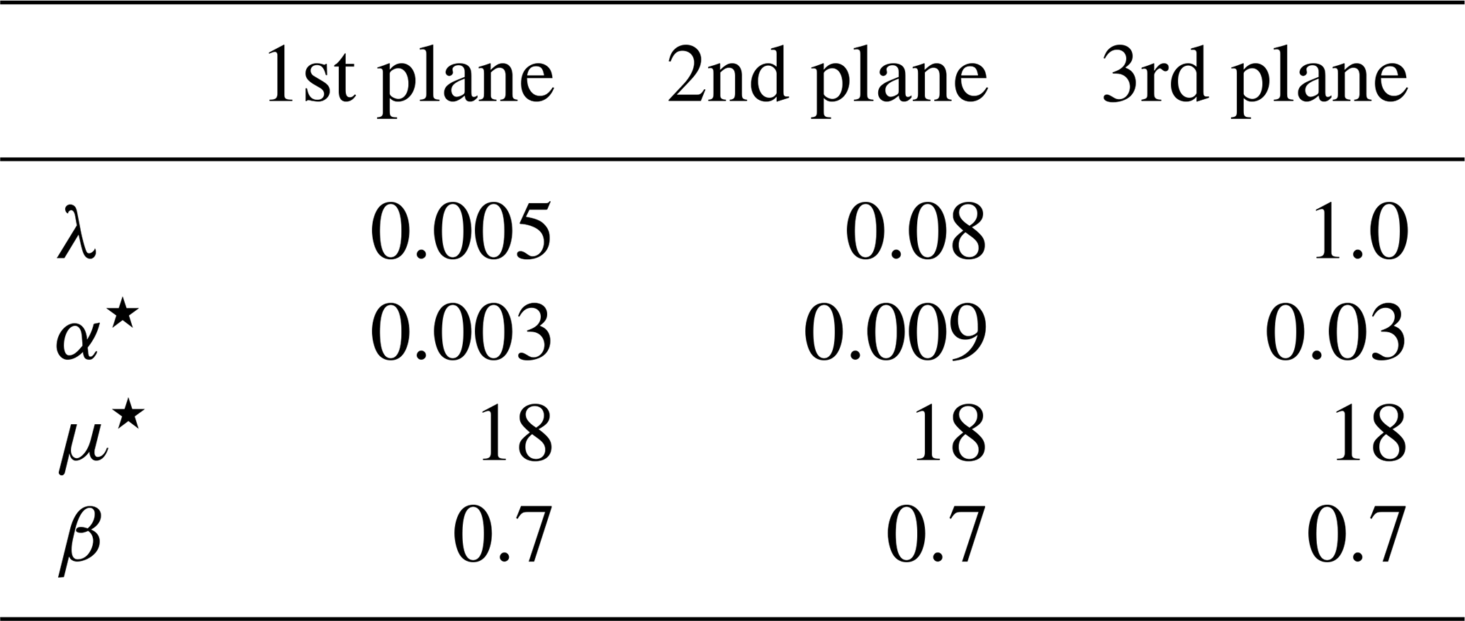
Note that a higher α^⋆ value for the finest ES plane results in a particularly high smoothing for areas that are sparsely covered with data. This means that the responses from the finest grid become flat in areas that have some distance to the next flight line.

4.2.3 Assumed data uncertainties

The assumed data uncertainties range between 5 nT for uniform high-quality datasets (e.g., AEROMAG, AEM) and 50 nT for datasets with poor quality and sparser data (e.g., GAP91/92, GICAS, EASTMAR, NOO-73). Because the data uncertainties represent the data weights in the inversion, it is possible to govern the impact of individual datasets onto the inversion results (e.g., data of flight lines are down-scaled in areas with little data coverage to avoid generation of elongated anomalies that are oriented along flight line directions). Used estimates for the data uncertainties in the southwestern area are shown as an example in Fig. 3.

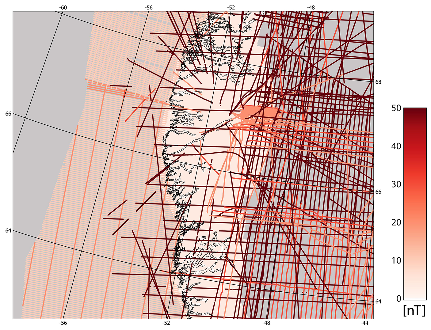
Figure 3 Used data uncertainty estimates at the southwestern block (same area is shown as in Fig. 5).

4.2.4 Corrections of constant shift bias

Each of the 50 aeromagnetic datasets was corrected for a separate constant shift during the inversion of the ES modeling. This approach allowed for the removal of systematic discrepancies in data levels between different surveys.

A special treatment was required for the GAP91/92 survey. It consists of a coarse pattern of lines, where individual lines are generally not well leveled. Because of that, many of its lines exhibit systematic biases relative to data from other surveys, with variations occurring from line to line. To address these inconsistencies, we applied individual shift corrections to each line within the GAP91/92 dataset.

In the same way, also a few of the ICEBRIDGE lines show such systematic bias relative to other surveys, and individual shift corrections are also applied to these lines.

4.2.5 Simulation of the magnetic anomaly

The magnetic anomaly is simulated in a uniform grid with 400 m spacing at a constant height of 2000 m a.s.l. (WGS84).

The spacing of the simulated grid was chosen to be slightly finer than that of the finest ES grid, ensuring that it is sufficiently detailed to allow the effective application of a low-pass filter during post-processing to remove residual dipole characteristics (see Sect. 4.4).

A constant height is used to present observed anomalies consistently for the complete magnetic compilation. The height is, moreover, chosen rather low to minimize resolution losses due to larger distances from the sources.

Note that a few mountain peaks have slightly higher elevations than 2000 m in Greenland, so that the assumption for the Laplace's equation is here not valid in a strict sense. However, in practice, the equivalent sources of the finest plane are located in a depth of 2 km such that short wavelengths typically associated with magnetization along the surface can not be fitted in the inversion. Accordingly, the equivalent sources mainly contain information from larger depths, and a simulation to a shallow height level is not critical.

4.3 Setup to handle large data sets

A main issue of ES modeling for large-scale compilation is that the matrix A is very large and requires some kind of treatment so that sufficient memory is available on a conventional PC, and, at the same time, allowing the calculations to be performed sufficiently quickly. Therefore, we choose a strategy where the computation time and required memory are kept acceptably low:

• First, data were resampled at 1 km data spacing in flight line direction, before using them as input in the ES modeling (Fig. 2). In this way, the number of data points used in the ES modeling could be significantly reduced (from ≈138 M to ≈1.8 M) without losing resolution in the ES modeling, since the new data sampling is in the range of the grid spacing (700 m) and depth (2.5 km) of the finest ES plane.

• Second, we do not use the full dense matrices A, but sparse matrix versions, and we solve the linear system with a LSQR sparse matrix solver (Paige and Saunders, 1982). Only sensitivities A_mn are considered for which

  $$a_{mn}<F_{\mathrm{dist}}\mathrm{\Delta }{x}_{\left(k\right)}$$

  with a_mn are the Euclidean distances between the dipoles and observation points and Δx_(k) is the grid spacing. The factor F_dist is chosen to be so large (at least >30) that the inaccuracies of the approximation are very small.

• Third, we divide the whole Greenland area into several overlapping blocks (9 blocks) and perform the equivalent source modeling separately in each block. Hereby, sizes of the blocks range from 0.5 to 1.5 M km² and the overlaps of neighboring blocks range from 120 to 230 km. This significantly reduces the number of dipoles and data points used in each inversion and, hence, also the overall computational time. So, the computation of ES modeling and following-up simulation takes about one day for an average sized block with a PC having a CPU with 32 processing cores and 4 GHz clock speed per core, but it would take more than a month to run the whole Greenland area with the same parameters using the same computer resources. After simulating the magnetic anomalies and integrating the long wavelengths from the satellite data, the magnetic anomaly maps of the individual blocks are merged into the final Greenland compilation by using the grid knit tool in Oasis Montaj (see flowchart in Fig. 2).

4.4 Post-processing

After equivalent source modeling, low-pass filters with cutoff wavelengths of 20, 5, and 1.5 km are applied to the grid of the simulated magnetic anomaly components of the coarse, medium, and fine ES plane, respectively (Fig. 2). These filters remove some very small remaining artificial patterns associated with the dipole characteristics. (Note that the cutoff wavelengths of these Fourier-based filters are very short and accordingly do not have any measurable distortions due to the spherical shape of the Earth.)

Then, the grids of the simulated magnetic anomaly components from the three ES planes are summed to obtain the final total magnetic anomaly. In a final step, the total magnetic anomaly grids of the different blocks are merged to the final compilation by using the grid knitting method in the software Oasis Montaj and areas with very low data coverage are cut out. It turns out that it is totally unproblematic to combine the different blocks with grid stitching at this late stage, because overlapping parts are very similar since the same data and the same methodology are used to produce the magnetic anomalies of the different blocks. In particular, the long-wavelength components are almost identical by using our precise SH approach to incorporate the satellite data.

5 Presentation of the magnetic anomaly compilation and evaluation of its quality

The final magnetic anomaly compilation of Greenland is presented in Fig. 4. Depending on the data coverage, different amounts of details are shown in the map. So, in large parts of the central and northern inland ice region, only long-wavelengths anomalies are visible due to the low data coverage (Fig. 1), but in most other regions more detailed short-wavelengths features are present. Particularly detailed information (wavelengths down to ≈2 km) is given in areas that are covered with the high-resolution AEROMAG datasets at the ice-free coastal areas of western, southern, and southeastern Greenland.

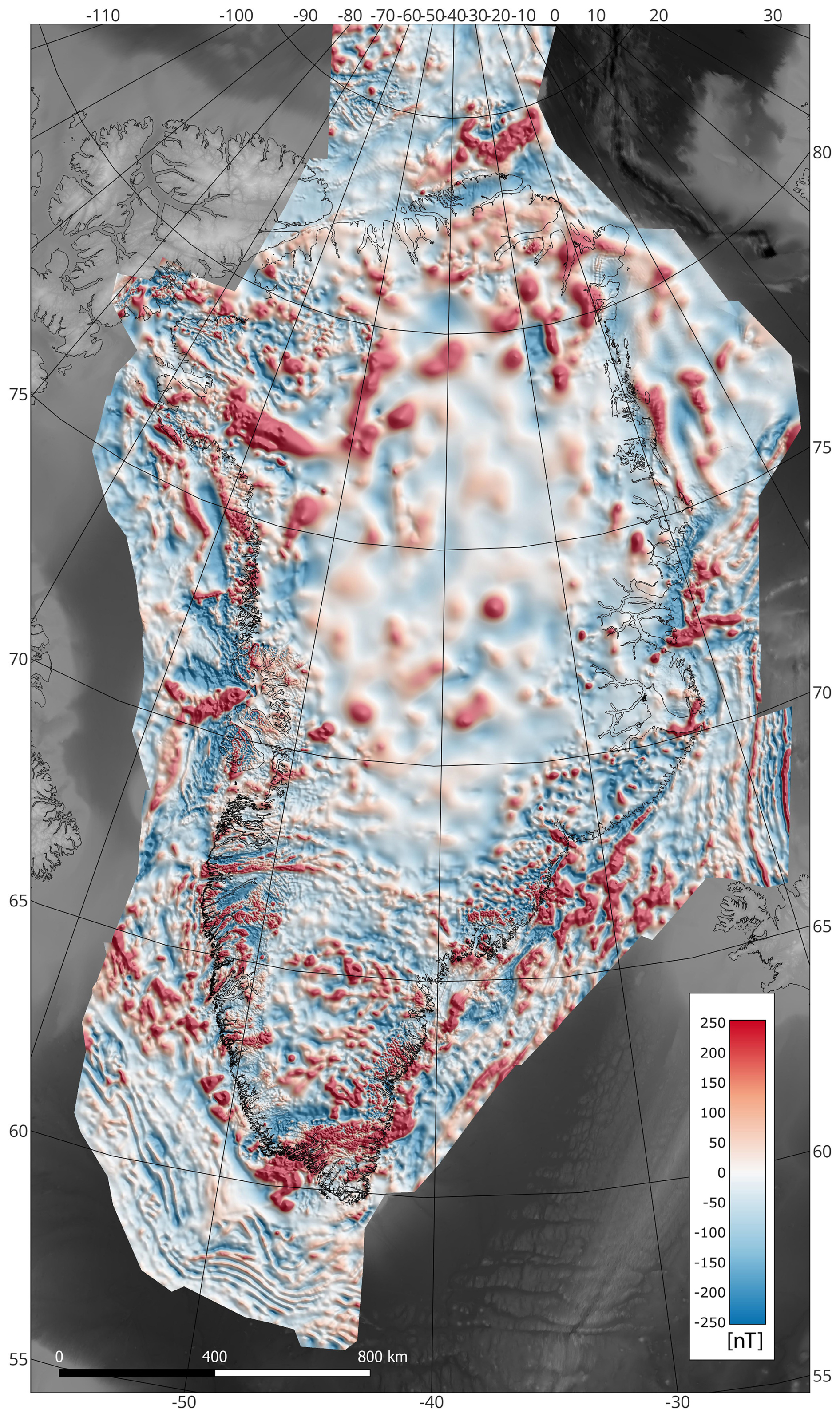
Figure 4 The final magnetic anomaly compilation GREENMAG.

5.1 Data uncertainties and data fits

When inversions without constant shift corrections are performed, several datasets are not well-fitted and biased data are responsible for artifacts in the resulting magnetic anomaly maps. This is illustrated in Fig. D1 for the Southwestern block. Here, it seems that in particular the lines of the GAP91/92 have systematically too large values, which could originate from an inadequate removal of the core field or a lack of base station corrections. This results in both positive data misfits d_calc−d_obs for these lines and the appearance of elongated artifacts in the magnetic anomaly map along some of these lines.

If the constant shift correction is now active in the inversion, most systematic data misfits along the lines are removed, and no obvious artifacts are observed any longer (Fig. 5). This example demonstrates the importance of correcting for shifts between datasets in the ES approach.

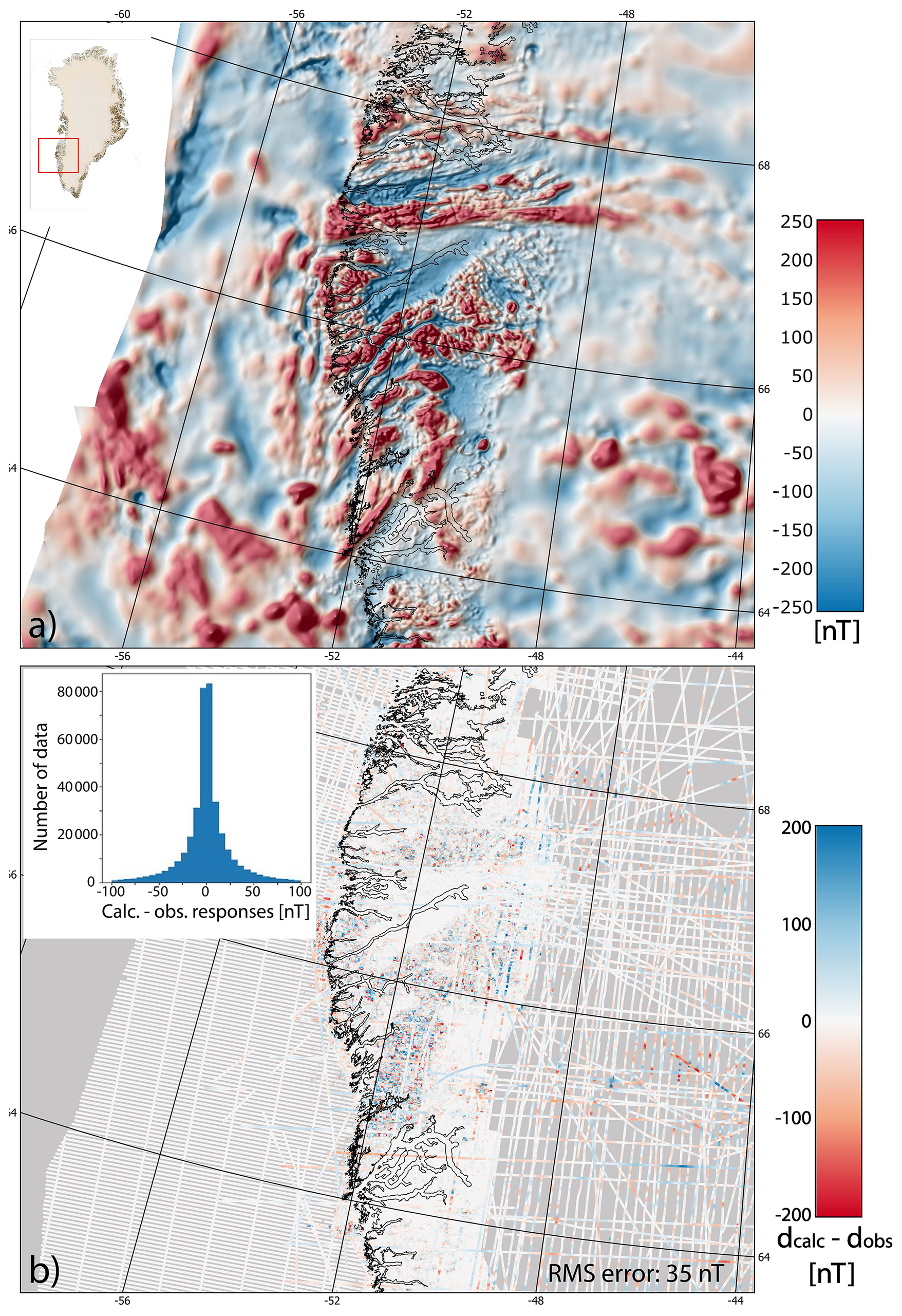
Figure 5 (a) Magnetic anomaly from the ES modeling for the southwestern block. (b) Data misfit between the observed and calculated data. The histogram in the upper corner presents the distribution of errors.

RMS data misfits for the final inversions with active shift corrections range between 21 and 73 nT for the different blocks, and error distributions for all blocks are symmetrical and centered at zero (Fig. 5). The data misfits are relatively high as very short wavelength variations from the near-surface in the high-resolution datasets (e.g., AEROMAG, AEM) cannot be fitted by equivalent sources located at depths of at least 2 km and having spacings of at least 700 m. Finer spacings of the equivalent sources are not used because of the increase in required memory and computation times. Furthermore, it becomes more demanding to keep the inversion stable in regions that have low data coverage if the ES spacing is made even finer.

In offshore regions, where magnetic stripping patterns are present, it can be assumed that remanent magnetization dominates and that polarity reversals of the Earth magnetic field during the time of rock formation are responsible for the changes in the remanent magnetization and hence observed magnetic anomalies. It is noteworthy that the data are generally good fitted in these regions, even though our equivalent source model assumes that all magnetization is solely induced (see Eq. 2). This suggests that our ES model provides reliably results even in regions that are dominated by remanent magnetization.

5.2 Compilation with and without using the finest equivalent source plane

Instead of the anomaly map presented in Fig. 4, where resolution is heavily dependent on the varying data coverage, one might prefer a map with a more uniform resolution. In this case, an option is to omit the responses simulated from the finest ES plane and present only the responses of the medium and coarse ES planes (see Fig. 6 as an example from South Greenland and Fig. C1).

Since the ES modeling of the finest plane is most sensitive to outliers in the data, the version from the medium and coarse ES planes also turned out to be numerically more robust against potential artifacts.

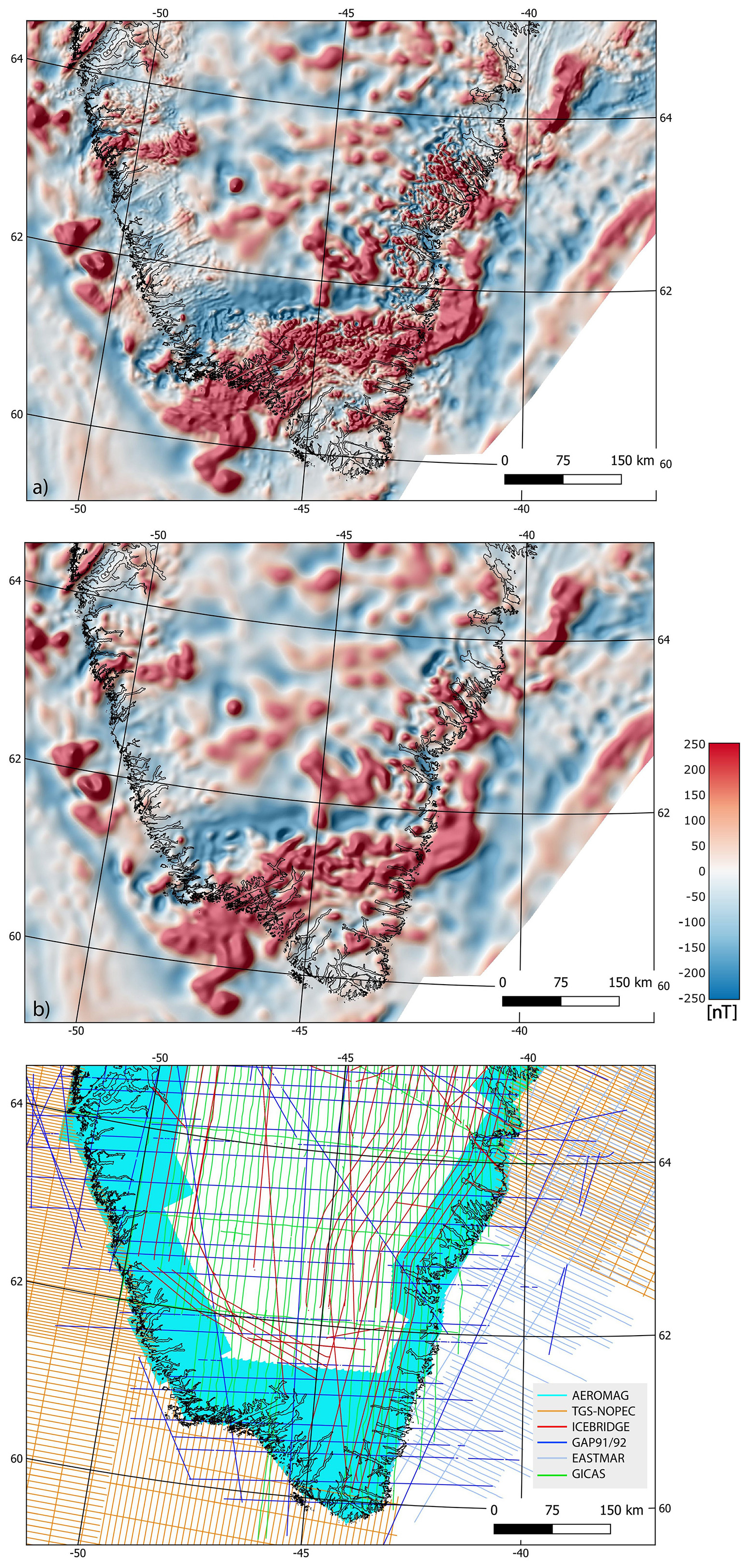
Figure 6 (a) shows the magnetic anomaly data, where the equivalent sources from all planes are used in the simulation, but (b) shows the magnetic anomaly, which is only based on the coarse and the medium ES plane. Note that both simulated data responses are similar in areas with lower data coverage (see data points in c), but areas covered by the high-resolution AEROMAG surveys show more details, when all ES planes are considered.

5.3 Replacement with satellite data

Figure 7 shows for the most southern block how the long-wavelength components (n= 13–133) from the aeromagnetic data are replaced by data from the LCS-1 satellite model. It can be seen by comparing Fig. 7c and d that the overall long-wavelength trend is significantly modified but that shorter-wavelength anomalies remain unchanged.

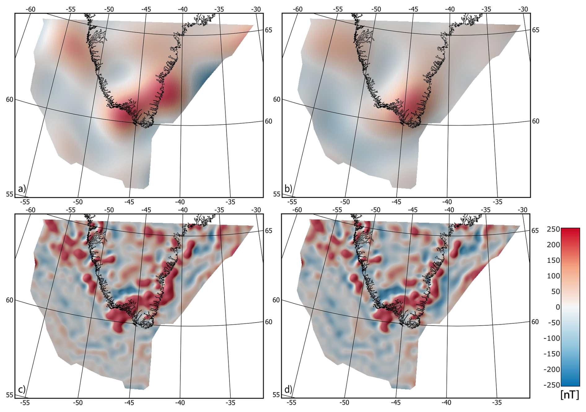
Figure 7 (a) and (b) show the long-wavelength components from the aeromagnetic data and the LCS-1 satellite model (degree of Gauss coefficients n= 13–133), respectively. Hereby, the long-wavelength components in (a) are determined directly from the dipole sources of the coarsest ES plane using the method of Dilixiati et al. (2022). (c) and (d) show the simulated magnetic anomaly data of the coarsest ES plane before and after these long wavelengths of the satellite model are replaced.

Since the long-wavelength contributions of the neighboring blocks become very consistent by replacement with satellite data, it is unproblematic to merge the different overlapping blocks together with grid stitching.

Although the replacement of long-wavelength components is straightforward, it is important to note that our approach does not account for potential inaccuracies in the satellite data itself. This means that it is assumed that satellite data are not significantly affected by errors in the long-wavelength range (n<133). However, this assumption may not always hold true – particularly at high latitudes, where external magnetic signals from persistent polar ionospheric current systems introduce elevated noise levels, and as a result, the resolution of small-scale lithospheric magnetic features in these regions can be degraded (Lesur and Maus, 2006). Therefore, we plan to modify the approach in the future so that it can account for inaccuracies for both the aeromagnetic and satellite data.

5.4 Comparison with the CAMP-M compilation

CAMP-M published in 2011 is the most recent magnetic compilation that covers all of Greenland (see Fig. E1). Therefore, it is natural to compare it with our new GREENMAG map. For completeness, we, moreover, present the magnetic anomaly map of the GAMMA-5 compilation (Verhoef et al., 1996) in Fig. F1.

Across the central to northern inland ice area (30–50° W and 70–77° N) characterized by low data coverage, it seems that the CAMP-M compilation generally shows some more details than the GREENMAG compilation (compare Figs. 4 and E1). This region is almost only covered by the sparse data from the GAP91/92 project (Fig. 1) that were used in both compilations, such that data availability is similar in both compilations, and the adapted smoothing regularization in the ES modeling of the GREENMAG compilation may reduce here the short-wavelengths content of some anomalies. On the other hand, the question arises if all the presented details in the CAMP-M are here really supported by the sparse data or if they are mainly the product of interpolation of data information along the lines into areas uncovered by data.

In all other regions, which are more densely covered with data, the GREENMAG compilation exhibits at least similar and in many places more details than the CAMP-M compilation. Figures 8 and 9 present two examples from northwest and southeast Greenland, where the new magnetic anomaly compilation provides much more details than the CAMP-M compilation.

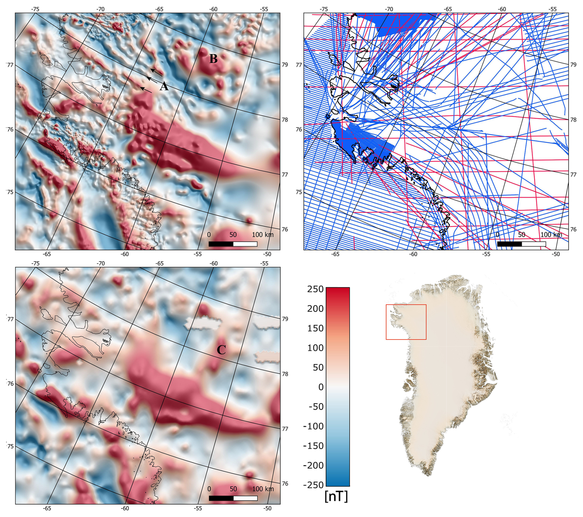
Figure 8 The magnetic anomaly of (a) the new GREENMAG compilation and (b) the CAMP-M compilation (Gaina et al., 2011) are shown for the northwestern part of Greenland (illumination for shading from NE). (c) Only data shown in red are used for the CAMP-M compilation, but both red and blue colored data points are used in the new compilation.

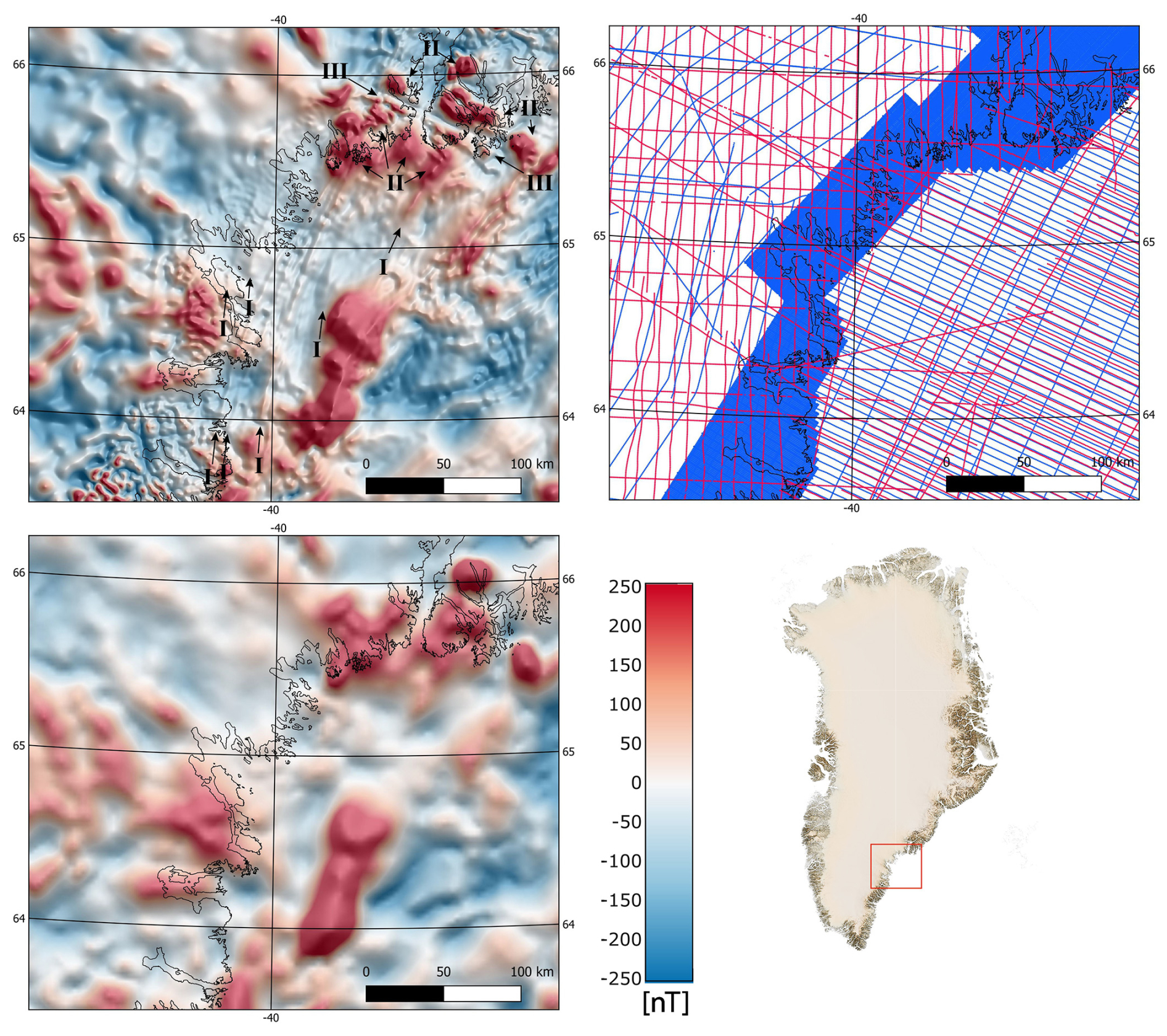
Figure 9 The magnetic anomaly data of (a) the new GREENMAG compilation and (b) the CAMP-M compilation (Gaina et al., 2011) are shown for the southeastern part of Greenland (illumination for shading from NE). (c) Only data shown in red are used for the CAMP-M compilation, but both red and blue colored data points are used in the new compilation.

In the northwestern area (Fig. 8) many elongated trends under the inland ice become present in the new compilation that are not resolved in the CAMP-M compilation (see e.g., A in Fig. 8). In addition, the shape of anomaly B is better defined in the new compilation, but anomaly C is not observed. The main reason for resolving here more details is that many of the datasets (ICEBRIDGE, TGS-NOPEC, AEM and Melville Bugt surveys) are not used in the CAMP-M compilation (see blue lines in Fig. 8c). This example demonstrates that more magnetic data in the inland ice region have the potential to much improve interpretations of subglacial geology.

In the south-eastern area (Fig. 9), the parts covered by the high-resolution AEROMAG datasets are much better resolved in the new compilation, since these datasets are not used in the CAMP-M compilation. But also in the remaining parts, the amount of presented details is higher in the GREENMAG compilations, since data from other datasets (ICEBRIDGE, TGS-NOPEC) are only used in this new compilation. In this area, several narrow elongated anomalies are visible in the new compilation (see I and III in Fig. 9a), which are not resolved in the CAMP-M compilation. The SSW-NNE subparallel trending positive anomalies I can be followed in the GREENMAG compilation over several hundreds of kilometers and are described as dykes of presumably Paleogene age (Riisager and Rasmussen, 2014; Heincke and Møller Stensgaard, 2017). The E–W trending magnetic low III is located immediately north of an igneous complex (Ammassalik Intrusive Complex) and is interpreted as the magnetic expression of a regional Proterozoic suture zone (of the Nagssugtoqidian Orogen) (Drenth et al., 2023). In the northeast part of Fig. 9, moreover, a pattern of several rounded anomalies (II) is resolved in much more detail in the GREENMAG compilation. The locations and shapes of these anomalies coincide well with mapped Proterozoic intrusions and a batholith in the northern and southern part, respectively (Kolb, 2014; Drenth et al., 2023).

6 Data availability

The magnetic anomaly maps of Greenland (GREENMAG) can be downloaded from the GEUS DataVerse website https://doi.org/10.22008/FK2/LQN5YJ (Heincke and Szwillus, 2025). Two types of maps are available. One is based on the ES of all three planes, but the other is based only on the ES of the first and second planes. This means that the first map shows more details in areas with a large data coverage. The maps are given as grids with an UTM zone 24 complex projection and a WGS84 datum (ESRI: 102574).

7 Conclusions

We present a new magnetic anomaly map for Greenland that is based on equivalent source modeling combined with spherical harmonic expansion. Our approach allows to consistently combine magnetic datasets with very different acquisition parameters and data quality in a way that the final magnetic compilation presents anomalies with a flexible and properly adapted resolution. It is, moreover, possible to separate the short, medium and long wavelengths contributions from each other by using three grid planes with largely different spacings (10, 2 and 0.7 km) and depth levels (40, 10 and 2.5 km) of the equivalent sources. Finally, it is straightforward to precisely incorporate long-wavelength information from satellite data by determining the Gauss coefficients associated with the aeromagnetic data directly from the equivalent sources and replacing high degrees (n= 13–133) with those from the satellites.

We show that the new magnetic anomaly map has in many areas of Greenland a significantly higher resolution than the former CAMP-M compilation and many features become visible in the new compilations not observed in these former compilations. The reasons for this are the availability of new datasets not used in the former compilation, but also the way the data are combined in the ES modeling (i.e. use of the actual point data).

The new GREENMAG magnetic anomaly map is expected to refine future interpretations of the regional Greenland geology both under ice cover as e.g., for estimation of the ice sheet basal conditions and heat flow, and the shelf regions, as e.g., for the breakup history and reconstruction of the plate tectonic movements. So, an earlier version of this compilation was already used as input of a joint inversion with gravity data to resolve the lithospheric structures under the inland ice of South Greenland (Wansing, 2024).

In the future, we intend to extend the established database with newly available magnetic datasets in Greenland. When sufficient new data are available, we will re-run the ES modeling to make an update of the GREENMAG magnetic anomaly map.

Appendix A: Implementation of the constant shift correction in the inversion

In the following, it is described how constant shift corrections are implemented in the inversion scheme. Assuming that we have V different surveys with $M^{\left(\mathrm{1}\right)},M^{\left(\mathrm{2}\right)},\mathrm{\dots },M^{\left(V\right)}$ data points (with $M=M^{\left(\mathrm{1}\right)}+M^{\left(\mathrm{2}\right)}+\mathrm{\dots }+M^{\left(V\right)}$), then the data term Φ_d of the objective function in Eq. (5) changes to:

$${\mathrm{\Phi }}_d=\left|\right|\mathbf{D}(\mathbf{A}\mathit{m}+\stackrel{\mathrm{̃}}{\mathit{d}}-\mathit{d})|{|}^{\mathrm{2}}$$

where

$$\stackrel{\mathrm{̃}}{\mathit{d}}=[\underset{M^{\left(\mathrm{1}\right)}\mathrm{elements}}{\underbrace{{\stackrel{\mathrm{̃}}{d}}^{\left(\mathrm{1}\right)},\mathrm{\dots },{\stackrel{\mathrm{̃}}{d}}^{\left(\mathrm{1}\right)}}},\underset{M^{\left(\mathrm{2}\right)}\mathrm{elements}}{\underbrace{{\stackrel{\mathrm{̃}}{d}}^{\left(\mathrm{2}\right)},\mathrm{\dots },{\stackrel{\mathrm{̃}}{d}}^{\left(\mathrm{2}\right)}}},\mathrm{\dots },\underset{M^{\left(V\right)}\mathrm{elements}}{\underbrace{{\stackrel{\mathrm{̃}}{d}}^{\left(V\right)},\mathrm{\dots },{\stackrel{\mathrm{̃}}{d}}^{\left(V\right)}}}{]}^T$$

is a vector that contains the constant shifts ${\stackrel{\mathrm{̃}}{d}}^{\left(\mathrm{1}\right)},{\stackrel{\mathrm{̃}}{d}}^{\left(\mathrm{2}\right)},\mathrm{\dots },{\stackrel{\mathrm{̃}}{d}}^{\left(V\right)}$ for the different surveys. These shifts can be associated with V additional model parameters $[{\stackrel{\mathrm{̃}}{m}}^{\left(\mathrm{1}\right)},{\stackrel{\mathrm{̃}}{m}}^{\left(\mathrm{2}\right)},\mathrm{\dots },{\stackrel{\mathrm{̃}}{m}}^{\left(V\right)}{]}^T=\stackrel{\mathrm{̃}}{\mathit{m}}$ with:

$$\begin{array}{}\text{(A1)}& {\stackrel{\mathrm{̃}}{d}}^{\left(v\right)}=\stackrel{\mathrm{̃}}{w}{\stackrel{\mathrm{̃}}{A}}^{\left(v\right)}{\stackrel{\mathrm{̃}}{m}}^{\left(v\right)}\mathrm{for}\mathrm{all}v=\mathrm{1},\mathrm{\dots },V.\end{array}$$

The constant $\stackrel{\mathrm{̃}}{w}$ is set by the user to define the overall effect of the shifts in the inversion, but constants ${\stackrel{\mathrm{̃}}{A}}^{\left(v\right)}$ are used for normalization, so that the shifts are balanced relative to the mean sensitivity of a data point belonging to the corresponding survey:

$${\stackrel{\mathrm{̃}}{A}}^{\left(v\right)}={\displaystyle \frac{\mathrm{1}}{M^{\left(v\right)}}}\sum _{m\in M^{\left(v\right)}}\sum _{n=\mathrm{1}}^N\left|A_{mn}\right|$$

Then, the kernel matrix and the model vector can be modified as follow:

$${\mathbf{A}}_{\mathrm{shift}}=\left(\begin{array}{ccccccc}& & \stackrel{\mathrm{̃}}{w}{\stackrel{\mathrm{̃}}{A}}^{\left(\mathrm{1}\right)}& \mathrm{0}& \mathrm{\dots }& \mathrm{\dots }& \mathrm{0}\\ & & \mathrm{⋮}& \mathrm{⋮}& & & \mathrm{⋮}\\ & & \stackrel{\mathrm{̃}}{w}{\stackrel{\mathrm{̃}}{A}}^{\left(\mathrm{1}\right)}& \mathrm{0}& \mathrm{\dots }& \mathrm{\dots }& \mathrm{0}\\ & & \mathrm{0}& \stackrel{\mathrm{̃}}{w}{\stackrel{\mathrm{̃}}{A}}^{\left(\mathrm{2}\right)}& \mathrm{0}& \mathrm{\dots }& \mathrm{0}\\ \mathbf{A}& & \mathrm{⋮}& \mathrm{⋮}& & & \mathrm{⋮}\\ & & \mathrm{0}& \stackrel{\mathrm{̃}}{w}{\stackrel{\mathrm{̃}}{A}}^{\left(\mathrm{2}\right)}& \mathrm{0}& \mathrm{\dots }& \mathrm{0}\\ & & \mathrm{⋮}& & \mathrm{\ddots }& & \\ & & \mathrm{0}& & & \mathrm{0}& \stackrel{\mathrm{̃}}{w}{\stackrel{\mathrm{̃}}{A}}^{\left(v\right)}\\ & & \mathrm{⋮}& & & \mathrm{⋮}& \mathrm{⋮}\\ & & \mathrm{0}& & & \mathrm{0}& \stackrel{\mathrm{̃}}{w}{\stackrel{\mathrm{̃}}{A}}^{\left(v\right)}\end{array}\right)$$

and

$${\mathit{m}}_{\mathrm{shift}}=[m_{\mathrm{1}},\mathrm{\dots },m_N,{\stackrel{\mathrm{̃}}{m}}^{\left(\mathrm{1}\right)},\mathrm{\dots },{\stackrel{\mathrm{̃}}{m}}^{\left(V\right)}{]}^T.$$

If in addition the constraint matrix C is changed to C_shift by padding V rows with 0-values, Eq. (6) becomes:

$$\begin{array}{}\text{(A2)}& {\mathit{m}}_{\mathrm{shift}}=({\mathbf{A}}_{\mathrm{shift}}^T{\mathbf{D}}^T{\mathbf{DA}}_{\mathrm{shift}}+{\mathit{\lambda }}^{\mathrm{2}}{\mathbf{C}}_{\mathrm{shift}}^T{\mathbf{C}}_{\mathrm{shift}}{)}^{-\mathrm{1}}{\mathbf{A}}_{\mathrm{shift}}^T{\mathbf{D}}^T\mathbf{D}\mathit{d}.\end{array}$$

In this setup relative constant shifts between surveys are now assigned to the model variables ${\stackrel{\mathrm{̃}}{m}}^{\left(\mathrm{1}\right)}$,…, ${\stackrel{\mathrm{̃}}{m}}^{\left(P\right)}$, and calculated data are obtained by

$${\mathit{d}}_{\mathrm{calc}}={\mathbf{A}}_{\mathrm{shift}}{\mathit{m}}_{\mathrm{shift}}.$$

A remaining problem is that there is an ambiguity in the combination of shifts solving the least square problem. Since the overall (data) shifts should be minimal, we remove this ambiguity by adding the following constraint to the objective function:

$$\begin{array}{}\text{(A3)}& {\mathrm{\Phi }}_{m,\mathrm{shift}}={\mathit{\lambda }}_{\mathrm{shift}}^{\mathrm{2}}\left|\right|\mathbf{R}(\stackrel{\mathrm{̃}}{\mathit{m}}-{\stackrel{\mathrm{̃}}{\mathit{m}}}_{\mathrm{ref}})|{|}^{\mathrm{2}}\to \min \mathrm{!},\end{array}$$

where R is a (V×V) diagonal matrix

$$R_{vv}={\displaystyle \frac{{\stackrel{\mathrm{̃}}{\mathit{\lambda }}}_{\mathrm{norm}}^{\left(v\right)}}{{\stackrel{\mathrm{̃}}{\mathit{\lambda }}}_{\mathrm{norm}}}}$$

with

$${\stackrel{\mathrm{̃}}{\mathit{\lambda }}}_{\mathrm{norm}}^{\left(v\right)}={\displaystyle \frac{\mathrm{1}}{N}}\sum _{n=\mathrm{1}}^N\sum _{m\in M^{\left(v\right)}}\left|\right(A_{mn}|$$

and

$${\stackrel{\mathrm{̃}}{\mathit{\lambda }}}_{\mathrm{norm}}={\displaystyle \frac{\mathrm{1}}{N}}\sum _{n=\mathrm{1}}^N\sum _{m=\mathrm{1}}^M\left|\right(A_{mn}|.$$

The R_vv have the intention to properly balance all individual data sets having very different amount of data points and, hence, also overall sensitivities.

A component in the reference vector ${\stackrel{\mathrm{̃}}{m}}_{\mathrm{ref}}^{\left(v\right)}$ is defined by the associated wished data shift ${\stackrel{\mathrm{̃}}{d}}_{\mathrm{ref}}^{\left(v\right)}$ (see Eq. A1). For the first grid layer, it is obvious that all ${\stackrel{\mathrm{̃}}{d}}_{\mathrm{ref}\left(\mathrm{1}\right)}^{\left(v\right)}\to \mathrm{0}$ such that

$${\stackrel{\mathrm{̃}}{\mathit{m}}}_{\mathrm{ref}\left(\mathrm{1}\right)}=\mathbf{0}.$$

In the Kth grid layer, for all separate shifts ${\stackrel{\mathrm{̃}}{d}}_{\mathrm{ref}\left(K\right)}^{\left(v\right)}\to {\sum }_{k=\mathrm{1}}^{K-\mathrm{1}}-{\stackrel{\mathrm{̃}}{d}}_{\left(k\right)}^{\left(v\right)}$ since the overall data shifts should be constrained toward zero (i.e., ${\stackrel{\mathrm{̃}}{d}}_{\left(\mathrm{1}\right)}^{\left(v\right)}+\mathrm{\dots }+{\stackrel{\mathrm{̃}}{d}}_{\left(K\right)}^{\left(v\right)}\to \mathrm{0}$). Using Eq. (A1), this results in:

$${\stackrel{\mathrm{̃}}{m}}_{\mathrm{ref}\left(K\right)}^{\left(v\right)}={\displaystyle \frac{{\sum }_{k=\mathrm{1}}^{K-\mathrm{1}}-{\stackrel{\mathrm{̃}}{w}}_{\left(k\right)}{\stackrel{\mathrm{̃}}{A}}_{\left(k\right)}^{\left(v\right)}{\stackrel{\mathrm{̃}}{m}}_{\left(k\right)}^{\left(v\right)}}{{\stackrel{\mathrm{̃}}{w}}_{\left(K\right)}{\stackrel{\mathrm{̃}}{A}}_{\left(K\right)}^{\left(v\right)}}}\mathrm{for}\mathrm{all}v=\mathrm{1},\mathrm{\dots },V$$

When Φ_m,shift (Eq. A3) is added to the objective function, the modified linear solution from Eq. (A2) is:

$$\begin{array}{}\text{(A4)}& \begin{array}{rl}{\mathit{m}}_{\mathrm{shift}}& =({\mathbf{A}}_{\mathrm{shift}}^T{\mathbf{D}}^T{\mathbf{DA}}_{\mathrm{shift}}+{\mathit{\lambda }}^{\mathrm{2}}{\mathbf{C}}_{\mathrm{shift}}^T{\mathbf{C}}_{\mathrm{shift}}\\ & +{\mathit{\lambda }}_{\mathrm{shift}}^{\mathrm{2}}{\mathbf{R}}_{\mathrm{shift}}^T{\mathbf{R}}_{\mathrm{shift}}{)}^{-\mathrm{1}}{\mathbf{A}}_{\mathrm{shift}}^T{\mathbf{D}}^T\mathbf{D}\mathit{d}\\ & +{\mathit{\lambda }}_{\mathrm{shift}}^{\mathrm{2}}{\mathbf{R}}_{\mathrm{shift}}^T{\mathbf{R}}_{\mathrm{shift}}{\mathit{m}}_{\mathrm{shift},\mathrm{ref}}\end{array}\end{array}$$

with

$${\mathbf{R}}_{\mathrm{shift}}=\left(\begin{array}{cccccc}\mathrm{0}& \mathrm{\dots }& \mathrm{0}& & & \\ \mathrm{⋮}& & \mathrm{⋮}& & & \mathbf{R}\\ \mathrm{0}& \mathrm{\dots }& \mathrm{0}& & & \end{array}\right)$$

having 0-values in the first N columns, and

$${\mathit{m}}_{\mathrm{shift},\mathrm{ref}}=[\mathrm{0},\mathrm{\dots },\mathrm{0},{\stackrel{\mathrm{̃}}{m}}_{\mathrm{ref}}^{\left(\mathrm{1}\right)},\mathrm{\dots },{\stackrel{\mathrm{̃}}{m}}_{\mathrm{ref}}^{\left(V\right)}{]}^T.$$

Appendix B: Spherical harmonic expansion for an equivalent source plane

Spherical surface harmonics are functions that are defined on spheres and are, furthermore, solutions of Laplace's equation. Accordingly, the potential Ω (with $\mathit{B}=-\mathrm{\nabla }\mathrm{\Omega }$) at the locations P^⋆ having the spherical coordinates $(r^{\star },{\mathit{\varphi }}_r^{\star },{\mathit{\theta }}_r^{\star })$ can be expressed by a series of spherical surface harmonics as:

$$\begin{array}{}\text{(B1)}& \begin{array}{rl}\mathrm{\Omega }(r^{\star },{\mathit{\varphi }}_r^{\star },{\mathit{\theta }}_r^{\star })& =r_{\mathrm{s}}\sum _{n=\mathrm{0}}^{\mathrm{\infty }}{\left({\displaystyle \frac{r_{\mathrm{s}}}{r^{\star }}}\right)}^{n+\mathrm{1}}\sum _{m=\mathrm{0}}^n(g_n^m\cos m{\mathit{\varphi }}_r^{\star }\\ & +h_n^m\sin m{\mathit{\varphi }}_r^{\star }\left)P_n^m\right(\cos {\mathit{\theta }}_r^{\star })\end{array}\end{array}$$

as long as all magnetic sources are located on or below r_s and $r^{\star }>r_{\mathrm{s}}$. Here, n and m are the degree and order of the spherical surface harmonics, respectively, $P_n^m\left(\cos \mathit{\theta }\right)$ are the associated Schmidt quasi-normalized Legendre polynomials, and $(g_n^m,h_n^m)$ are the Gauss coefficients to weight the individual spherical surface harmonics in the expansion.

By determining the gradient of Eq. (B1), the components of the associated B-field can be written as a series of SHs:

$$\begin{array}{}\text{(B2)}& \begin{array}{rl}{B}_{r^{\star }}& =\sum _{n=\mathrm{0}}^{\mathrm{\infty }}{\left({\displaystyle \frac{r_{\mathrm{s}}}{r^{\star }}}\right)}^{n+\mathrm{2}}\sum _{m=\mathrm{0}}^n(n+\mathrm{1})(g_n^m\cos m{\mathit{\varphi }}_r^{\star }\\ +& h_n^m\sin m{\mathit{\varphi }}_r^{\star }\left)P_n^m\right(\cos {\mathit{\theta }}_r^{\star })\\ B_{{\mathit{\varphi }}_r^{\star }}& =\sum _{n=\mathrm{0}}^{\mathrm{\infty }}{\left({\displaystyle \frac{r_{\mathrm{s}}}{r^{\star }}}\right)}^{n+\mathrm{2}}\sum _{m=\mathrm{0}}^{n}m(g_n^m\sin m{\mathit{\varphi }}_r^{\star }\\ & -h_n^m\cos m{\mathit{\varphi }}_r^{\star })\left[{\displaystyle \frac{\mathrm{1}}{\sin {\mathit{\theta }}_r^{\star }}}{P}_n^m\left(\cos {\mathit{\theta }}_r^{\star }\right)\right]\\ B_{{\mathit{\theta }}_r^{\star }}& =-\sum _{n=\mathrm{0}}^{\mathrm{\infty }}{\left({\displaystyle \frac{r_{\mathrm{s}}}{r^{\star }}}\right)}^{n+\mathrm{2}}\sum _{m=\mathrm{0}}^n(g_n^m\cos m{\mathit{\varphi }}_r^{\star }\\ & +h_n^m\sin m{\mathit{\varphi }}_r^{\star })\left[{\displaystyle \frac{\partial P_n^m\left(\cos {\mathit{\theta }}_r^{\star }\right)}{\partial \mathit{\theta }}}\right]\end{array}\end{array}$$

Dilixiati et al. (2022) have shown in their paper that the contributions of an individual magnetic dipole to the Gauss coefficients (and hence to a magnetic field) can be directly determined and are given as:

$$\begin{array}{}\text{(B3)}& {\displaystyle }\begin{array}{rl}{g}_{n,s}^m& ={\displaystyle \frac{\mathit{\chi }V}{\mathrm{4}\mathit{\pi }{r_{\mathrm{s}}}^{\mathrm{3}}}}\left(n{B}_{r_{\mathrm{s}}}\cos m{\mathit{\varphi }}_{\mathrm{s}}{P}_n^m\left(\cos {\mathit{\theta }}_{\mathrm{s}}\right)\right.\\ & -{\displaystyle \frac{m{B}_{{\mathit{\varphi }}_{\mathrm{s}}}}{\sin {\mathit{\theta }}_{\mathrm{s}}}}\sin m{\mathit{\varphi }}_{\mathrm{s}}{P}_n^m\left(\cos {\mathit{\theta }}_{\mathrm{s}}\right)\\ & \left.+B_{{\mathit{\theta }}_{\mathrm{s}}}\cos m{\mathit{\varphi }}_{\mathrm{s}}{\displaystyle \frac{\partial P_n^m\left(\cos {\mathit{\theta }}_{\mathrm{s}}\right)}{\partial \mathit{\theta }}}\right)\end{array}\text{(B4)}& {\displaystyle }\begin{array}{rl}{h}_{n,s}^m& ={\displaystyle \frac{\mathit{\chi }V}{\mathrm{4}\mathit{\pi }{r_{\mathrm{s}}}^{\mathrm{3}}}}\left(n{B}_{r_{\mathrm{s}}}\sin m{\mathit{\varphi }}_{\mathrm{s}}{P}_n^m\left(\cos {\mathit{\theta }}_{\mathrm{s}}\right)\right.\\ & +{\displaystyle \frac{m{B}_{{\mathit{\varphi }}_{\mathrm{s}}}}{\sin {\mathit{\theta }}_{\mathrm{s}}}}\cos m{\mathit{\varphi }}_{\mathrm{s}}{P}_n^m\left(\cos {\mathit{\theta }}_{\mathrm{s}}\right)\\ & \left.+B_{{\mathit{\theta }}_{\mathrm{s}}}\sin m{\mathit{\varphi }}_{\mathrm{s}}{\displaystyle \frac{\partial P_n^m\left(\cos {\mathit{\theta }}_{\mathrm{s}}\right)}{\partial \mathit{\theta }}}\right),\end{array}\end{array}$$

where $(r_{\mathrm{s}},{\mathit{\varphi }}_{\mathrm{s}},{\mathit{\theta }}_{\mathrm{s}})$ are the locations of the dipoles Q in spherical coordinates. Summing up the contributions from all dipoles results in total Gauss coefficients:

$$\begin{array}{rl}& g_n^m=\sum _{s\in N}{g}_{n,s}^m\\ & h_n^m=\sum _{s\in N}{h}_{n,s}^m\end{array}$$

that can be used to calculate the B-field of an ES plane by using Eq. (B2).

Appendix C: Magnetic anomaly obtained from the coarse and medium plane

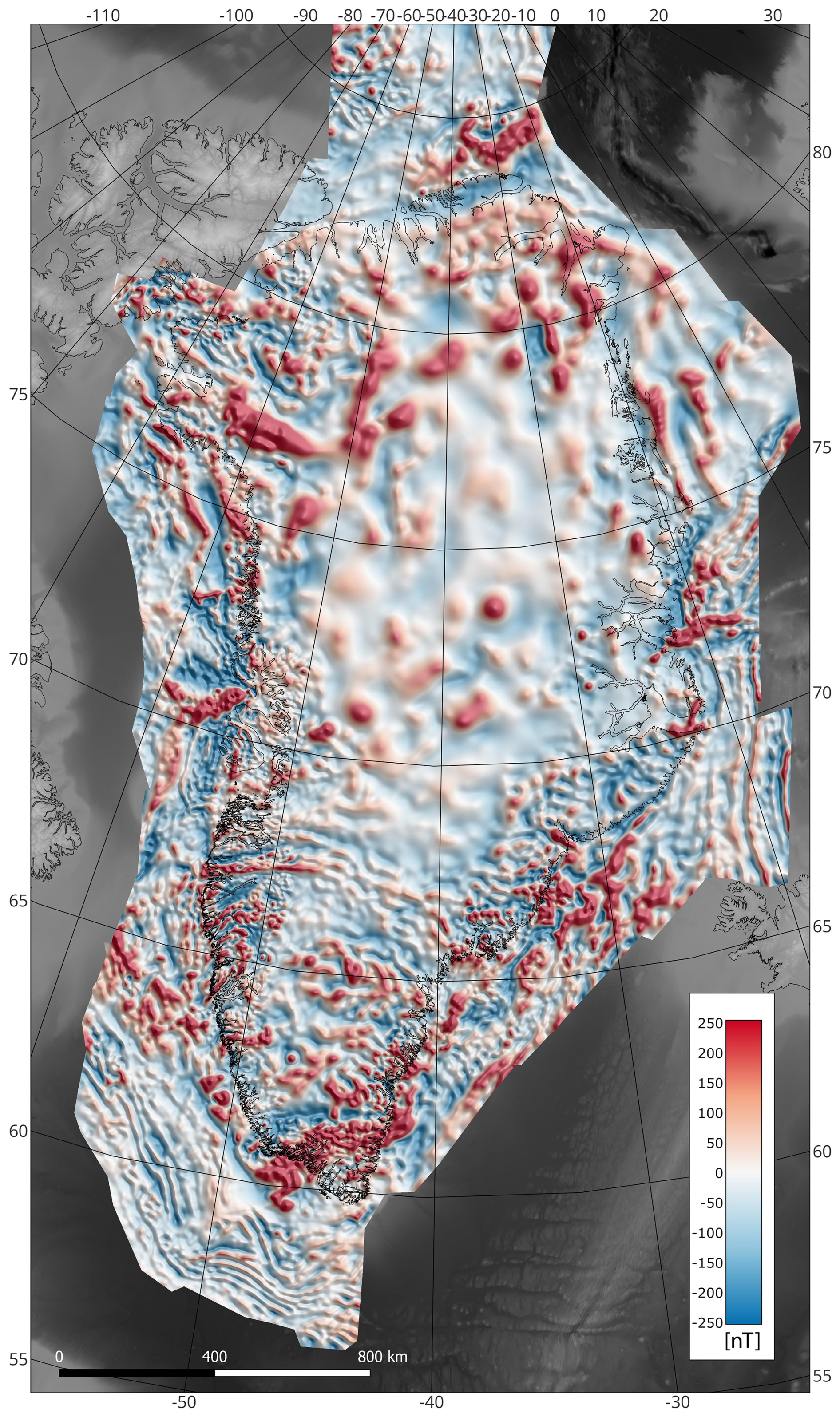
Figure C1 The magnetic anomaly map of the GREENMAG compilation, when only the equivalent sources of the coarse and medium plane are used for simulation.

Appendix D: Inversion results without constant shift correction

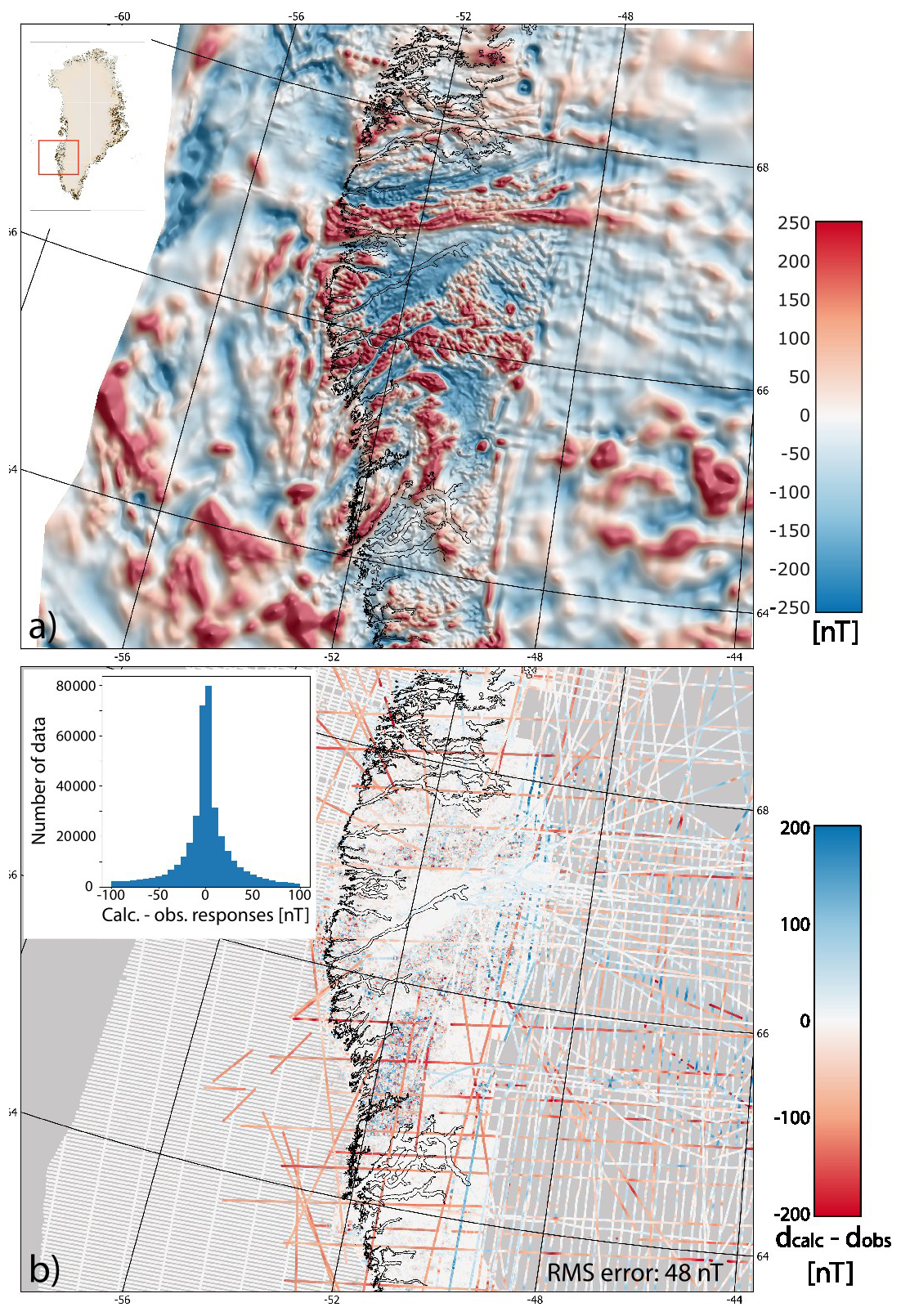
Figure D1 The same images as in Fig. 5, but here no constant shift corrections were applied in the inversion. (a) shows the magnetic anomaly from the ES modeling for the southwestern block and (b) shows data misfit between the observed and calculated data. The histogram in the upper corner presents the distribution of errors.

Appendix E: CAMP-M compilation

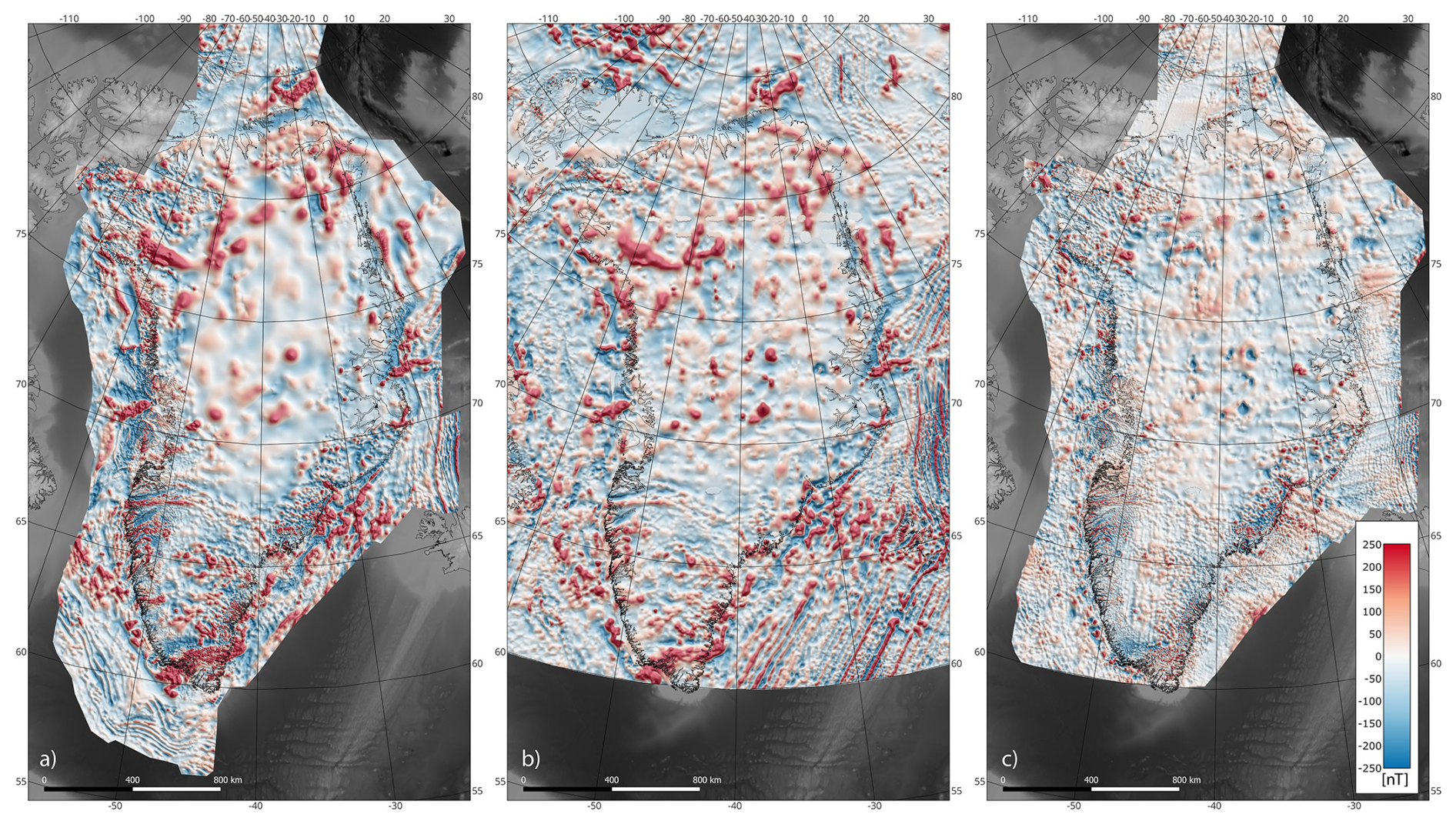
Figure E1 Magnetic anomaly maps from (a) GREENMAG and (b) Circum-Arctic Mapping Project (CAMP-M) (Gaina et al., 2011). (c) The difference of both maps.

Appendix F: GAMMA-5 compilation

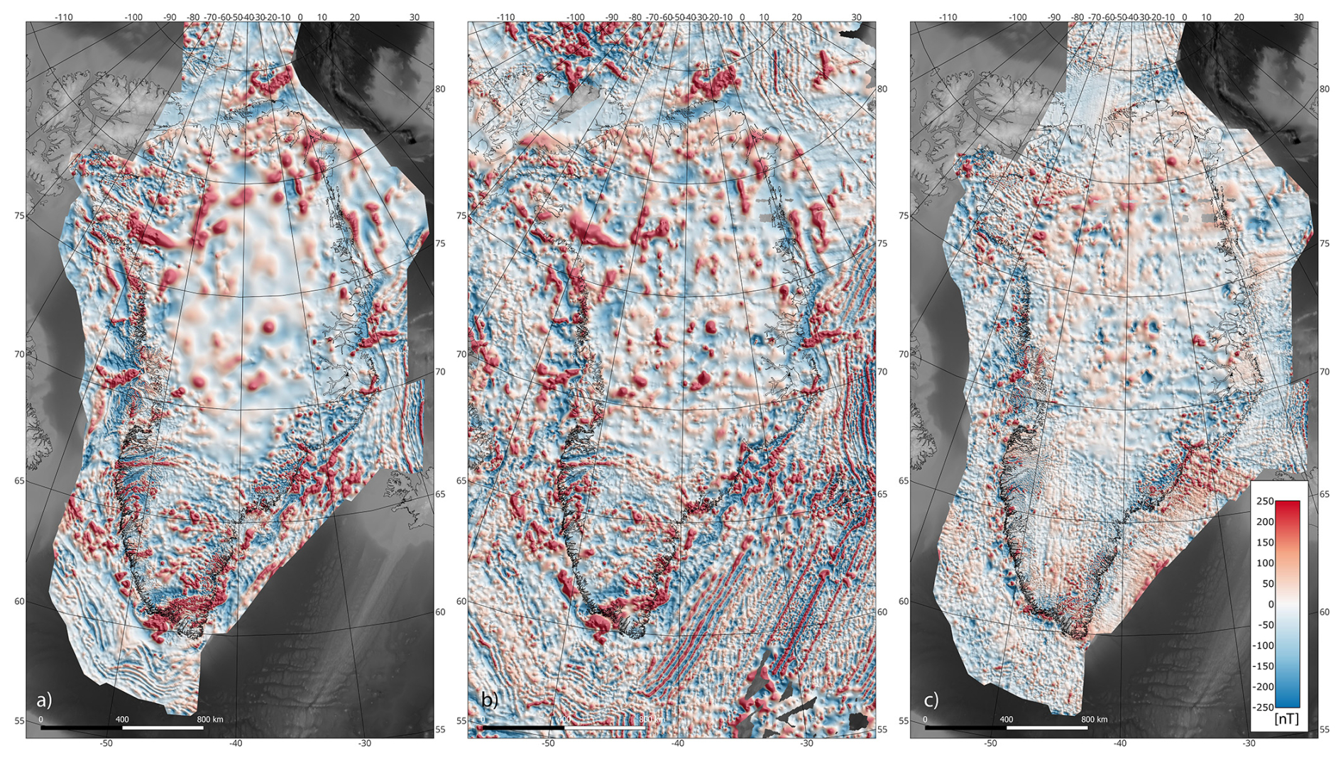
Figure F1 Magnetic anomaly maps from (a) GREENMAG and (b) GAMMA-5 (Verhoef et al., 1996). (c) The difference of both maps.