Continuous meteorological surface and soil records (2004–2024) at the Met Office surface site of Cardington, UK

A continuous meteorological and hydrological observational record is described for the Met Office semi-rural field site of Cardington in southern England between 2004 and 2024. The site was designed to carry out boundary layer, fog and air-surface exchange research to improve the representation of process-based physics within the Met Office Unified Model. The site lay in a flat river basin and was laid mainly to cropped grass and was surrounded by arable fields intermixed with small trees and shrubs through most wind sectors. Observations utilised flux masts at various heights, plus visibility, radiosondes, very near-surface and subsoil in situ sensors in addition to more specialist remote sensing instruments to retrieve atmospheric properties. In addition to boundary layer and surface data, soil properties such as temperature, moisture and water table depth were obtained. All components of the surface energy balance could be determined. Availability of data based on 30 min time steps over 20 years, for the combined components of the energy balance not flagged as either bad or missing, amounts to 77 %. The momentum roughness length as determined at the 10 m height for the prevailing wind sector remained near 3 cm from 2005–2022 but increased to 7 cm in 2023 and 2024 predominately due to growth in a 52 ha of woodland within 1 km of the site. An overview of the site, instrumentation, data availability, quality control, data storage at the UK CEDA repository, and potential uses of the dataset are described (https://doi.org/10.5285/5487380511084413a502c4b229273bc6, Met Office et al., 2025). A set of meteorological forcing files has also been compiled suitable for driving standalone land surface models configured for a single point.

1 Introduction

Geographically dispersed ground-based weather data from both professional and private (“citizen science”) automatic weather station sources are crucial to the initialisation and therefore operation of numerical weather prediction (NWP) models (Rawlins et al., 2007; Bell et al., 2015). Additionally, specialist surface sites at locations such as Cabauw in the Netherlands (Bosveld et al., 2020), the SIRTA observatory 20 km southwest of Paris, France (Chiriaco et al., 2018), the three fixed ARM sites of the Atmospheric Measurement Facility (Miller et al., 2016), and Cardington in southern England provide datasets for in-depth research in order to improve the physics within climate and NWP models. This can be achieved either via a statistical approach using long-term data, or special intensive observation periods (IOPs) lasting between hours and a few days, or a combination of both methods. Although a fixed surface site cannot be readily applied to large spatial scales, except via remote sensing with radars and lidars, it allows analysis over a wide range of time scales from minutes (e.g. fog development) to months or years (e.g. changes in deep soil moisture content). This allows for model forecast evaluation across a range of time scales as well as the development of parametrizations, whether these be full parametrizations or partially resolving such as within the turbulent grey zone (Wyngaard, 2004).

A key role of a land surface model (LSM) is to partition the surface energy balance via the fluxes of heat, moisture and radiation. Field sites that observe all components of the surface energy can be used in principle to test and improve the diagnostics simulated by LSMs. All components of energy exchange in an LSM, and their closure, are parametrised and essentially rely on a one-dimensional exchange of energy that is perpendicular to the surface. LSMs obey the conservation of energy at each time step, whereas the observations based on a number of different sensors do not: the observed energy balance should be treated as unclosed (Mauder et al., 2020a). That being said, in order to validate model output there are accepted methods to correct the observed energy balance to force closure. Twine et al. (2000) have demonstrated that eddy covariance systems are the largest cause of error for sites within relatively homogeneous terrain. With the net radiation and ground heat fluxes being deemed relatively accurate, the sensible and latent heat fluxes can be corrected by assuming the ratio of these fluxes, i.e. the Bowen ratio, is measured correctly. Although the heat fluxes archived from Cardington are uncorrected, and the energy balance residuals are small, we recommend using the method of Twine et al. (2000) if energy closure is required.

The importance of soil moisture on evapotranspiration and ground heat storage was one reason for installing subsoil sensors at Cardington. Historical observations of land surface evaporation are relatively scarce in contrast to precipitation and runoff data scarce (Blyth et al., 2010). Soil water content strongly modulates how the surface responds to atmospheric forcings. This should be borne in mind when carrying out long-term simulations using LSMs: the relatively slowly changing nature of soil water content compared to atmospheric time scales, means that following an anomalously wet period high soil water values can persist from weeks to seasonal time scales (e.g. Niu et al., 2011). A sensitivity study of the Met Office offline LSM by Osborne and Weedon (2021) during a strong seasonal drydown at Cardington shows the challenges in modelling evapotranspiration for a large dynamic range in soil water content.

Table 1 A modern history of research at Cardington – significant research projects leading to publications that use Cardington site data from between 2004–2024. IOP = Intensive Observation Period, VISURB = Visibility in Urban areas, LES = Large Eddy Simulation. Other abbreviations described in the caption of Fig. 5.

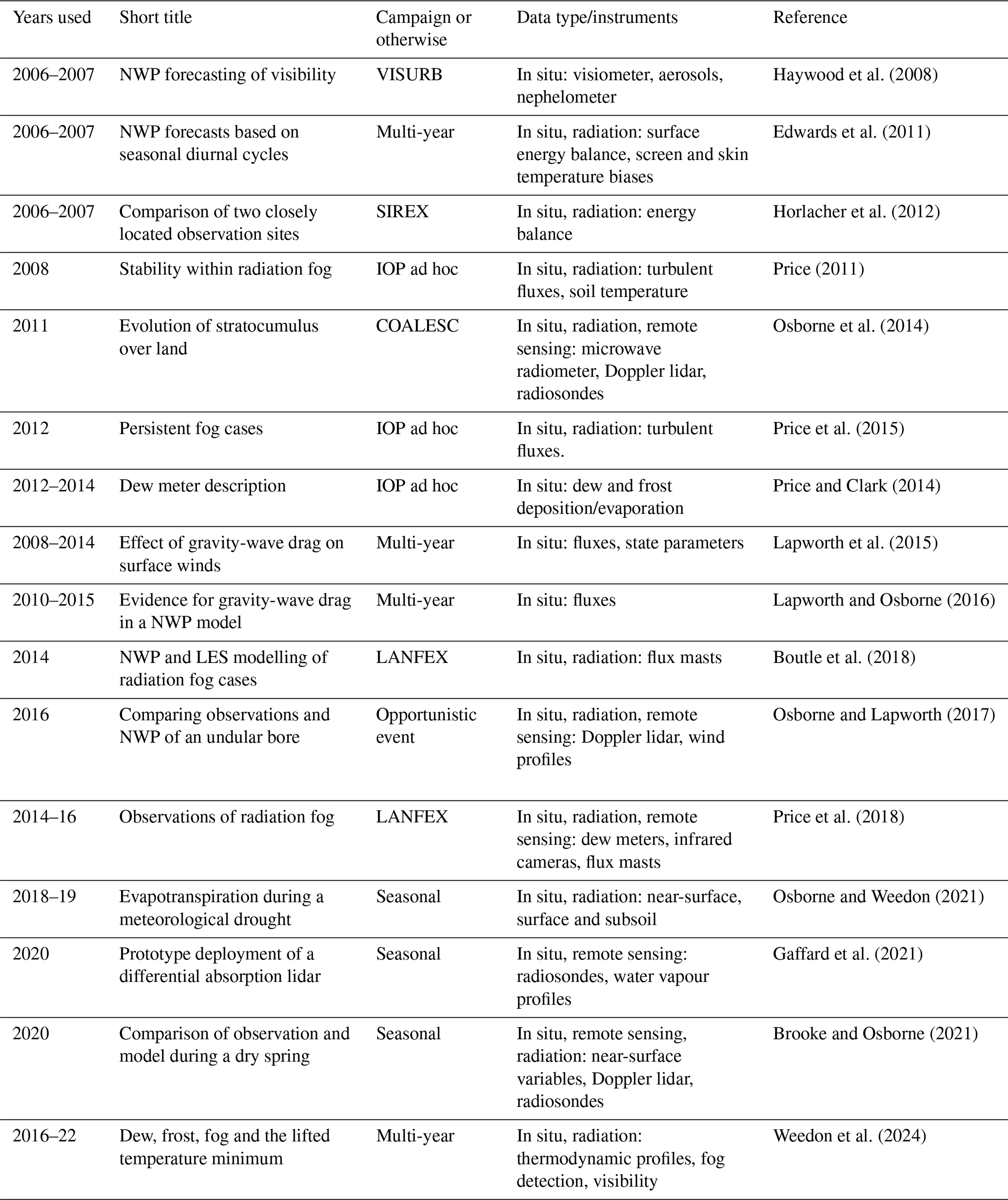
Cardington was established for both model evaluation (e.g. Price et al., 2018) and improvement of the parametrisations of processes in the Met Office LSM and regional NWP schemes (Boutle et al., 2014). Table 1 shows an illustrative list of published research from the past 20 years that focuses on site data. These projects tended to use a combination of both the continuous core meteorological dataset and more specialist instruments that were installed as remote-sensing technology allowed in-situ sensors to be augmented. Studies of the stable nighttime boundary layer (Horlacher et al., 2012), the morning and evening transitions (Angevine et al., 2020), and visibility (Haywood et al., 2008) have all been carried out over the past two decades. The perennial problem of fog forecasting was a recurring research theme at Cardington that has led to improvements in both LES and NWP modelling. Boutle et al. (2018) showed that attention needs to be paid to simulations of weak turbulence and low supersaturations that activate low concentrations of fog droplets. If this activation can be modelled using explicit aerosol data, then the evolution of optically thin, stable fog into thick, unstable fog can be better captured.

Despite such progress, however, there remains much untapped data and therefore potential research projects that the wider community is now welcome to address. Although some of the Cardington core meteorological data have previously been stored at a national archive (BADC) for the years 2006–2017, this dataset was limited in scope e.g. the soil sensors and turbulent fluxes were missing, had relatively poor quality control, little or no metadata, and was in ASCII. This former dataset has now been superseded by an exhaustive set of NetCDF files with comprehensive metadata compliant to CF-1.8 conventions. After a site description in Sect. 2, the core dataset comprising the meteorology, fluxes, radiation and subsoil properties is described in Sect. 3. This is followed in Sect. 4 covering how a LSM forcing dataset was derived from the core dataset. The specialist remote sensing lidars and microwave radiometers are described in Sect. 5, and the radiosonde archive is described in Sect. 6. The archived data described in Sects. 4, 5 and 6 have never been publicly available previously. An example use of the turbulence data is included in Sect. 7, and finally a description of the file formats and DOIs used in the archived products is shown in Sect. 8. These datasets can be downloaded from the UK Centre for Environmental Data Analysis (CEDA) repository for atmospheric and earth sciences observation data.

2 Site description

The Cardington 18 ha site in Bedfordshire southern England (52°06^′17.9^′′ N 0°25^′26.8^′′ W was the location of the 10 m flux tower in the centre of the site) has an elevation of 29 m ± 1 m above mean sea level and was laid mainly to manicured grass maintained at 5–10 cm height throughout the year. This area of the UK receives amongst the lowest rainfall of the country with around 550 mm a⁻¹, alongside 1320 h of annual sunshine and a peak monthly occurrence of radiation fog occurrence of 160 h based on the 20-year October average. The site sits within a broad (10 km), shallow valley that is a tributary of the River Great Ouse. The down-valley slope in general is about 0.15°. Although the immediate surroundings of the site are fairly flat, there is a ridge to the southeast with elevations of up to 100 m above mean sea level; this ridge runs southwest-northeast and passes within 5 km of the instrumented site at its closest approach. The screen and 10 m sensors were situated in the middle of the site to be as isolated as possible. An investigation by Grant (1994) showed that the modest terrain surrounding Cardington can, under certain conditions, influence the direction of the wind profiles. In the bottom 200 m of a stably stratified boundary layer – when the flow aloft has a component into the ridge – the surface flow can be channelled along the ridge. Under neutral and unstable conditions, however, this terrain effect becomes negligible.

The sector 030° through 280° is in general open fetch with arable fields with changing crop types (alternating wheat, rapeseed or left fallow, Fig. 1). The sector 280–350° is housing (> 1 km away) and sector 350–025° is dominated by the two large airship sheds (each 247 m long, 84 m wide and 55 m high) 400–600 m away. Consequently, wind and turbulence data should be analysed with caution when the wind direction comes from the direction of the hangars (350–025°) – though the majority of wind vectors lie outside this range (Fig. 1c). Satellite images of an area 2.5 km by 4.5 km with the site centred from 2003 and 2023 show dramatic differences in the colour of many of the fields in the image: due to changing crop types and the time of year the photographs were taken. The increase in urbanisation immediately to the north and preparation of an area for further housing immediately to the northeast are clearly seen. The hangars and an area called Shocott Spring are outlined in Fig. 1. Shocott Spring is an area of growing woodland situated in the sector 170–240° that was planted in stages from 2005 to 2011. This area now amounts to 52 ha, is 0.5–1.3 km away from Cardington. The change in turbulence due to the growth of these trees is discussed in Sect. 3. The wind rose in Fig. 1c, covering the years 2005–2009, indicates that the Shocott Spring woodland lies partially within the prevailing wind direction.

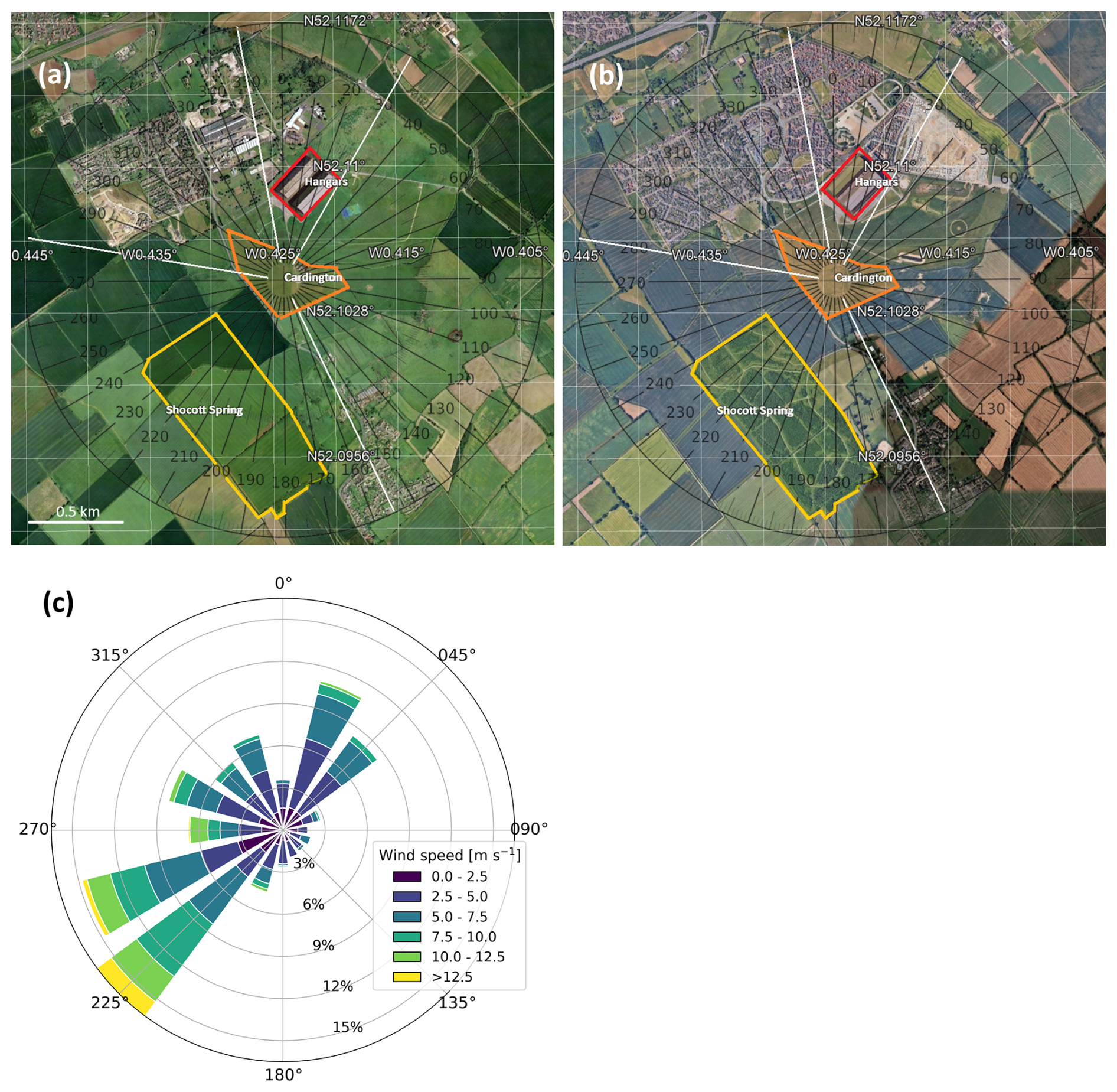
Figure 1 Satellite imagery with inlaid magnetic compass of the site location taken in (a) January 2003, and (b) August 2023. The airship hangars (red outline), Cardington site (orange) and Shocott Spring woodland (yellow) are annotated. (c) A wind rose calculated over the years 2005—2009 inclusive. Satellite Images courtesy of © Google Earth 2025 The GeoInformation Group and © 2025 Maxar Technologies.

The soils at the site are described geologically as loamy solifluction deposits over river valley gravels. Impervious Oxford Clay Formation underlies the whole area at an unknown depth. Soil sample analysis (Burton, 1999) shows that the topsoil (0–20 cm) is clay loam with 3 %–4 % intimate humus (organic matter), depths between 20 and 66 cm is medium clay loam (roughly equal fractions of clay, sand and soil), whilst deeper soil down to 170 cm is sandy gravel with 70 %–80 % sand content though locally there is chalky diamictite (boulder clay). The soil composition partially controls water infiltration, percolation, soil moisture content and evaporation. The vegetation canopy also affects infiltration and the plant water uptake – itself dependent on the moisture content within the rooting zone – controls transpiration. The exchange of water vapour between the soil and atmosphere is often a poorly constrained mechanism of LSMs and therefore is a weak link in the simulated hydrological cycle. Soil hydraulic properties can be derived from the observed soil composition, and such soil properties can be used to initialise LSMs; this is discussed in more detail in Sect. 4. A small stream runs through the research site which was situated to the north of all the instrumentation. Water table depth data (from two locations on the site labelled as “south” and “west”) shows that the hydraulic gradient, and hence the flow of subsurface water, is towards the stream despite the surface of the site being essentially flat.

3 Core instrumentation

3.1 Site set-up and data logging

The core hydrometeorology instrumentation for logging purposes was divided into six groups:

• i.

  50 m ultrasonic anemometer, temperature, humidity.

• ii.

  25 m ultrasonic anemometer, temperature, humidity.

• iii.

  10 m ultrasonic anemometer, temperature, fast hygrometer.

• iv.

  Broadband radiative fluxes

• v.

  “Screen-level” temperature, humidity, aerosol, visibility, pressure, rainfall and other miscellaneous; ultrasonic anemometer from 2011.

• vi.

  Subsoil profiles of moisture and temperature.

Data were logged almost continuously – allowing for sensor failure, calibration and power outages – between May 2004 and the end of 2024 creating the “core dataset”. Although data logging started in May 2004, the number of variables was initially limited as instrumental spin-up occurred over a period of a few months. Data prior to this period was stored in an archaic format deemed too costly to recover. The so-called “screen level” was set at a height of 1.2 m for pressure, temperature and humidity throughout the period. Although for logging purposes they were included in the “screen” data, the aerosol, visibility and present weather sensors (Sect. 3.2.6) were at 2 m, the rain-gauge was sited on the ground with the inlet rim at 0.45 m above the surrounding grass, and the sonic anemometer fitted in 2011 was also at 2 m. Therefore because of the large number of atmospheric variables at or below 2 m, the data in Fig. 2 for example has been split into “screen” and “2 m”, where “screen” refers to sensors at 1.2 m.

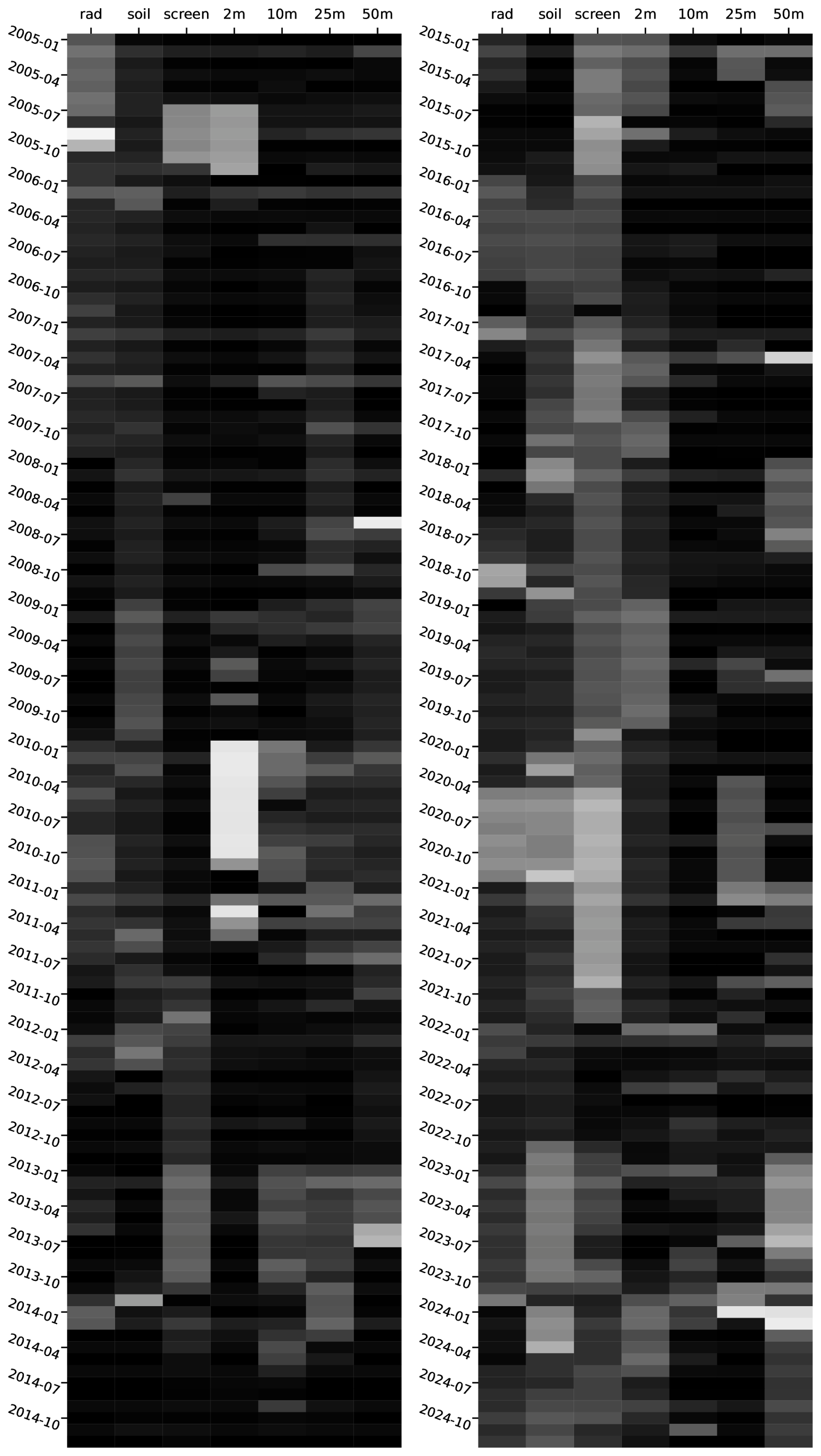
Figure 2 Data completeness divided into two 10-year periods for the core surface site instrumentation as split into “50 m”, “25 m”, “10 m”, “2 m”, “screen” (≤ 1.2 m) levels, and also “soil” (all buried subsoil sensors) and “rad” (radiative fluxes) categories. Each bar contains the data availability as a percentage of data not flagged as bad or missing (Table 2), graded on from white (0 %) to black (100 %).

All data were regularly transferred from the loggers to a central data storage computer. The central processing PC clock was routinely synchronised to an external Network Time Protocol (NTP) server, with the individual logger clocks in turn adjusted to the PC time. The data processing routines created four files per day i.e. for data averaged over periods of 1, 5, 10 and 30 min. These four timestep intervals have been preserved when creating the archived NetCDF files: therefore, apart from major data losses due to power cuts for example, there exist four NetCDF files per day for the core site variables throughout the 20-year period. Data from certain slow response sensors, like the soil sensors for example, are not included in the 1 min files; and we have only calculated variances and covariances from the mast data at 10 and 30 min. During relatively developed turbulence, 10 min is often sufficient to capture the majority of the turbulent energy and therefore derive reliable (co)variances (Raabe et al., 2002); otherwise in more benign conditions 30 min intervals are recommended that will capture most large scale, low frequency contributions (El-Madany et al., 2013).

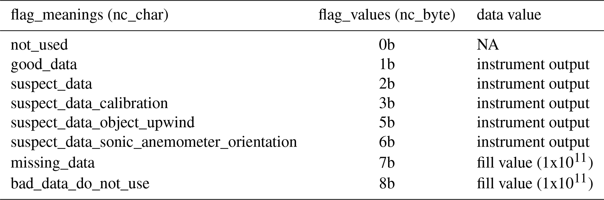
In addition to the sensors contributing to the core dataset, we had various microwave radiometers, lidars, ceilometers and disdrometer running at various times. These more specialist instruments were logged separately to the core data. Sometimes these additional instruments would be used elsewhere on detachment, so in general their use was not intended to be as continuous as the core instrumentation. They are described in more detail in Sect. 5. With the exception of a special subset of the core data for driving LSMs described in Sect. 4 there has been no gap-filling applied to either the core data or the additional data in Sect. 5. A system of quality flags has been used for the core data as listed in Table 2.

Table 2 Data flags used in the core hydrometeorology NetCDF files. NA: not applicable.

3.2 Core dataset instrumentation

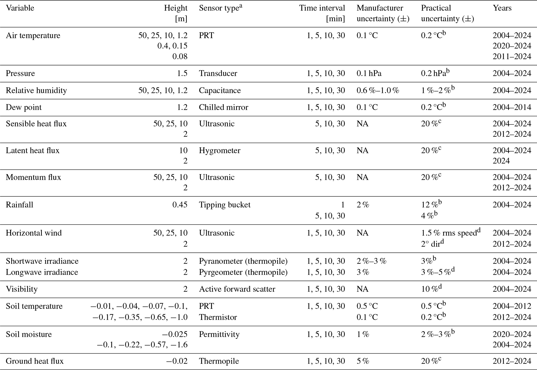
This section will provide details of core dataset instrumentation contained in the archived NetCDF files. Table 2 lists the data quality flagging system used in the archived files for the core dataset instrumentation. The principal meteorological and subsoil variables are summarised in Table 3 with uncertainties, as provided both by the manufacturer and as determined either locally or from the literature. We describe further pertinent deployment and calibration information below but see also Supplement Tables S1–S4 where details on sensor manufacturers and periods of deployment are listed. These tables are not exhaustive because the total number of variables is too large (180): the metadata in the NetCDF archive files should be scrutinised for details. Figure 2 shows data availability, i.e. percentage of data not flagged as missing or bad, organised by month and by meteorological level – all variables in Fig. 2 are divided into 50, 25, 10, and 2 m, screen, subsoil and radiation. This allows a basic grasp of how reliable the site was as function of time. We have split the data into two panels covering a decade each to improve legibility. To put Fig. 2 in some additional perspective, the data availability (i.e. not flagged as either bad “X” or missing “m”) of the components of the surface energy balance – latent heat flux at 10 m, sensible heat flux at 10 m, ground heat flux, net shortwave and longwave radiation and surface (grass) temperature – are 93.8 %, 96.0 %, 95.7 %, 95.5 % and 92.8 %, respectively, based on the 20-year dataset. The combined data availability of these components, i.e. the percentage of 30 min time steps where all the components are not flagged as bad or missing at the same time, is 81.9 %. When we in addition ignore data that is flagged as suspect (“?”) then this combined value becomes 77.5 %.

Table 3 Important core meteorological, radiation and subsoil variables with deployment heights, processed time interval and measurement uncertainties. ^a Further Details on the various instruments and their period of deployment are contained within Tables S1 (core meteorology), S2 (aerosol and visibility), S3 (radiation) and S4 (subsoil). ^b In-house calibrations. ^c From Cardington field evaluation. ^d Accepted error from the literature. NA: not available.

Overall confidence in the ability to observe the energy components is shown in Fig. 3 by the change in the energy balance residuals and the net downwelling and net upwelling energy, where each point is a yearly average. We do not include ground heat flux here despite the capability to estimate it. The subject of ground heat is a study in itself that requires careful corrections based on soil properties and water content. In addition, since the heat flux plates were deployed only from 2012, ground heat would have to be estimated from soil temperature profiles for some or all of the time series. Although we attempted this and the resulting trend in the residuals is broadly similar to Fig. 3a, with an increasing energy surplus in the last 10 years, the evolution was more erratic with greater dynamic range (i.e. greater apparent error) and so it was decided to leave the observed ground heat flux out of the calculation. Assuming a net zero ground heat flux over a full year is a common approach and is likely to be accurate for unchanging site conditions (Mauder et al., 2020a). The residual energy in Fig. 3a is close to zero for nine of the 20 years, with the range in residual energy spanning about 17 W m⁻². This is very small at only 3.8 % of the net downwelling radiation shown in Fig. 3b, although it amounts to roughly 40 % of the net available energy (not shown). The trend to an apparent energy surplus in the latter years coincides with increasing net downward radiation, which is caused by increases in both shortwave (≈ 10 W m⁻²) and longwave (≈ 5 W m⁻²) yearly means. These increases remain unexplained, but it is feasible they could be real and due to changes in cloud cover or they could be instrumental drift or bias.

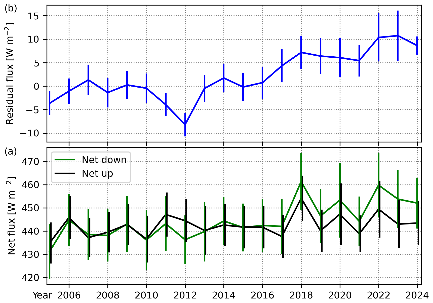
Figure 3 20-year time series of the annual mean (a) energy balance residual flux, and (b) net down and net up fluxes. Net down = [shortwave irradiance down + longwave irradiance down]; net up = [shortwave irradiance up + longwave irradiance up + sensible heat flux + latent heat flux]. Error bars are 95 % confidence intervals.

3.2.1 Sonic anemometers

The sonic anemometer sensor heights for masts heights nominally stated elsewhere as heights of 25 and 50 m were actually at 26.2 and 51.2 m above ground level. An extra sonic anemometer was installed at a height of 0.4 m in 2022. The thinking behind this was to investigate potential collapse of turbulence very close to the ground in stable nighttime conditions and hence demonstrate a form of decoupling from a turbulent regime at 2 or 10 m. This data remains an untapped resource. The sonics were logged using in-house software on Linux-based MOXA UC740 embedded computers while the remainder was logged using commercially available DT85-series data loggers manufactured by dataTaker. The DT85 could monitor a wide variety of analogue inputs (voltages, currents, resistances) at varying rates. One minute averaged data was logged based on a raw sampling rate of 0.5 Hz.

The Gill tri-axis ultrasonic anemometers have an asymmetrical design that ensures minimal flow distortion except for a small angle centred at the mount point. The manufacturer quotes accuracy of the u, v and w components of better than 1 % RMS (root mean square) for wind speeds between 0 and 45 m s⁻¹. When the wind direction was coming from the mast and mount of the sonic, it was flagged as such in the data (see Table 2). Although the sonics are capable of a 50 Hz processing rate, 10 Hz is sufficient to capture all the energy within the inertial subrange as it starts to blend into the dissipation frequencies (Mauder et al., 2020b). The orientation of the anemometer is logged in the header of the data files. Directions were measured with a compass and the bearing in degrees magnetic is noted. The magnetic variation can also be entered, and this is applied when calculating the true wind direction for the data display. The magnetic variation is not logged, so subsequent data processing routines were needed to take it into account to obtain the most accurate wind directions.

The additional sensors that were co-located with the sonics were connected to the analogue inputs of the sonic anemometers. These additional sensors were the platinum resistance (PRT) temperature sensors (at all heights), the humidity sensors (humicaps at 2, 25 and 50 m), and a Licor high-speed hygrometer (see Sect. 3.2.2). The PRTs were calibrated in-house to an accuracy of 0.1 °C. Table S5 provides a list of major changes of the four mast height deployments such as change of equipment, or updated calibration, usually involving the lowering and raising of the mast over a period of 1–2 h for the 2 and 10 m masts, or 1–2 d for the 25 and 50 m masts. The methodology for deriving kinetic turbulence fluxes (sensible heat, latent heat and momentum) alongside other variances from raw sonic data took the following sequence:

1. Read in raw hourly sonic data (36 000 lines).

2. Check for corrupt lines

3. If corrupt count > 50, then abort that file (no gap-filling), and flag as “missing data”

4. Read in sensor inclination and orientation, rotate coordinate matrices following Wilczak et al. (2001) so that means of u and v components are zero

5. read in calibration constants for analogue channels (PRT, humidity)

6. convert units (e.g. absolute to specific humidity)

7. filter for $u,v,w$ thresholds, apply quality flags

8. Remove outliers and apply linear detrend on $u,v,w$ components for appropriate time segments (5, 10, 30 min)

9. Calculate variances ($u^{\prime }{u}^{\prime },v^{\prime }{v}^{\prime },w^{\prime }{w}^{\prime },T^{\prime }{T}^{\prime }$) and covariances ($u^{\prime }{v}^{\prime },u^{\prime }{w}^{\prime },v^{\prime }w,u^{\prime }{T}^{\prime },w^{\prime }{T}^{\prime },w^{\prime }{q}^{\prime }$)

Although a PRT sensor was used as an absolute temperature measurement at each mast height, it is the fast-response sonic temperature that was used to calculate variances and covariances. This sonic temperature is related, but not identical, to virtual temperature and is derived from the measurement of the speed of sound (the principle of operation of the anemometer). Sonic temperature is suitable for monitoring variations because of a very short time constant but it is unsuitable as a measure of absolute air temperature. Offsets in sonic temperature from virtual and true temperature can amount to 0.5 and 2.4 °C, respectively, because of effects of humidity (Kaimal and Gaynor, 1991). When calculating turbulent fluxes, however, the effect of humid air on the variance of sonic temperature falls to the order of 0.01 °C or less than 2 % of the flux, well within a typical experimental error of 20 % (Horlacher et al., 2012). Users are of course welcome to apply temperature corrections if they wish, e.g. by following Foken et al. (2012). Correction for high frequency spectral losses in the data have not been carried out, although this could be attempted on the processed fluxes using the simplified analytical method of Massman (2000).

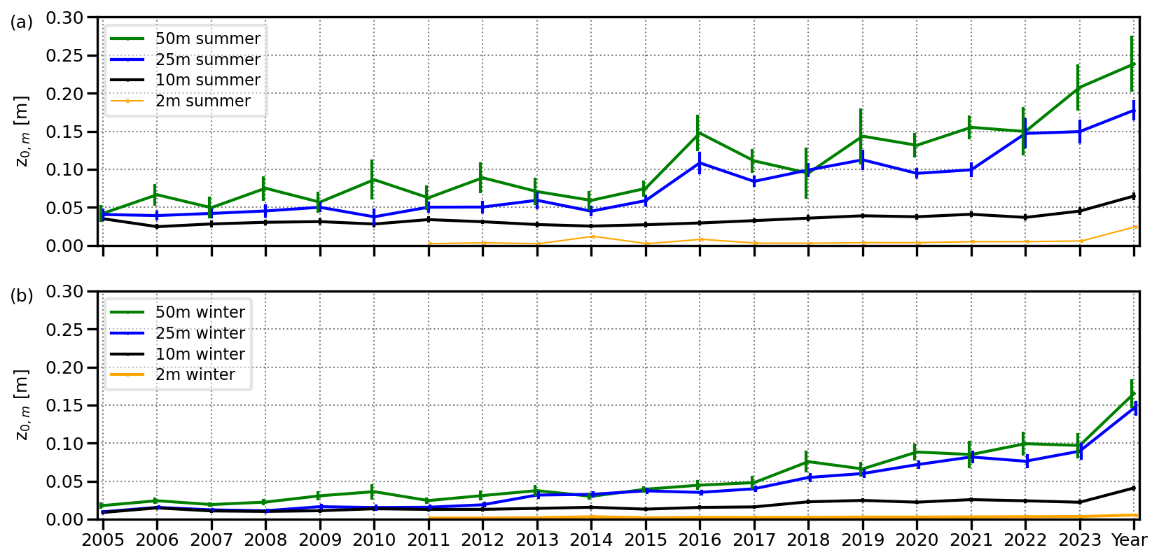
Figure 4 Evolution of the yearly median roughness lengths for momentum (z_0,m) as derived in neutral conditions from the four mast heights at Cardington. Only wind directions between 155 and 280° are included. Error bars show the 95 % confidence intervals. Data has been divided into the (a) summer and (b) winter months. Note the 2 m data only commenced in 2011.

Arguably the central component of the core dataset is the long-term turbulent fluxes measured at multiple mast heights. Confidence in these data is effectively combined in Fig. 4 with the effects of the surrounding land-use changes (Sect. 2). Here the median roughness lengths for momentum (z_0,m) derived using the high-frequency sonic anemometer data at 2, 10, 25 and 50 m are shown for the prevailing wind sector 155 and 280° that contains 58 % of the total turbulence dataset (see Fig. 1). In addition, only neutral conditions ($|z/L|\mathit{<}\mathrm{0.1}$ where L= Obukhov length, z= measurement height) are included here. Mast data at 2 m is only available from 2011. The two panels in Fig. 4 show z_0,m split into summer (June, July, August) and winter (December, January, February) months. The summer (“leafy”) months show larger values in z_0,m across the whole period at 10, 25 and 50 m. Importantly, z_0,m at 25 and 50 m show a significant increase in summer months from 2016 and in winter from 2018. Summer months show a slightly larger relative increase relative to winter, yet the winter period nonetheless shows an increase because bare trees also tend to increase turbulence. The change is only pronounced at 50 and 25 m due to the fetch of the woodland, with a significant increase at 10 m only in the last two years in summer. The change in time at 2 m is insignificant because derived z_0,m will be representative of turbulence generated within the site. Turbulence at 2 m in general is not developed and so values are small. It is interesting that the 10 and 25 m z_0,m values are about equal in winter between 2004 and 2012 after which the 25 m values start to rise. The larger z_0,m values at 25 m in the summer between 2004 and 2013 was probably due to growing crops in the surrounding fields that were harvested before winter. It is not until 2013 that the growing Shocott Spring trees irrevocably change the turbulence at 25 m relative to 10 m. In summary, although roughness lengths increased from 2013 for 25 and 50 m, at 2 and 10 m they remained essentially constant over the period apart from a slight increase at 10 m for 2023 and 2024.

3.2.2 Licor high speed hygrometer

The Licor-7500 hygrometer is an active near-infrared open-path instrument that detects changes in carbon dioxide and water vapour. Data was logged at 10 Hz, although the unit can log up to 20 Hz. The fundamental gas sampling rate is 150 Hz. The Li-7500 is not an absolute device and is designed primarily for variances of CO₂ and specific humidity and thereby covariances when collocated with a sonic anemometer, from which the latent heat flux can be estimated. The Licor was positioned at 10 m alongside the sonic anemometer for the duration of the dataset, mounted on a separate 1 m boom and offset laterally by about 45 cm from the sonic. An additional Licor was also deployed at 2 m (alongside the 2 m sonic anemometer) for seven months during 2024. It was hoped the latter would help elucidate the hard-to-measure moisture fluxes in stable conditions when the flux often hovers around zero, despite appreciable dew fall accumulations being observed at the surface (Osborne and Weedon, 2021). The 2 m moisture flux data remain unanalysed.

Coincident logging allowed the sensor outputs to be incorporated into the same data stream as the sonic data. This ensures accurate time synchronisation when calculating, for example, humidity covariances. For latent heat flux calculations, 10 m covariance using the Licor hygrometer should therefore be used as standard. This eddy covariance technique is the most common method globally for measuring evapotranspiration (Pastorello et al., 2020). A Webb-Pearman-Leuning scalar flux correction appropriate for open-path analysers, i.e. for the effect of water vapour on air density and additional thermal expansion effects, has not been applied to the latent heat fluxes in the archive. A post-processing correction can however be applied using the simplified recommendation of Jentzsch et al. (2021), although it is noted that corrections are typically no greater than a few % (compared to measurement error of about 10 %).

Yearly zeroing of the Li-7500 is achieved in the laboratory by using soda lime and magnesium perchlorate to scrub a controlled flow of CO₂ and water vapour, respectively. The Li-7500 contains similar internal scrubbers to void the sample optics of detection gases that were changed every year. The Li-7500 was mounted at a 15° angle so that rain or fog deposition water on the sapphire optics readily flows off; nonetheless, data during periods of precipitation or mist/fog should be treated as suspect. As with the sonic anemometer data, although the raw 10 Hz data for the Li-7500 are stored at the Met Office, the CEDA archive only contains the processed (co)variances (at 10 or 30 min time intervals) and the nominal mean specific humidity and CO₂ mixing ratio at all time intervals. Accuracy of the specific humidity of the Licor, based on the calibrations, is estimated as 0.2–0.3 g kg⁻¹, although this error could drift to larger unknown values between calibrations. The Licor CO₂ data in general remains to be exploited.

3.2.3 Relative humidity

The screened and aspirated HMP155s relative humidity (RH) sensors were mounted as standard at 50, 25, 10 and 1.2 m. For the near surface sensors at 40, 15 and 8 cm, the Hygroclip2 sensor (for both temperature and RH) was used. The 8 cm sensor effectively records the canopy temperature and RH, i.e. the air that is in contact with the grass blade tips. The 8 cm data collection began in 2014 whilst the 40 and 15 cm sensors were not deployed until 2021. The reason for deploying the Hygroclip2 sensors below the traditional screen height of 1.2 m was to investigate the thermodynamic conditions that lead to dew fall, fog (Price, 2019) and the lifted temperature minimum (Weedon et al., 2024). Two HMP155s were co-located at 25 and 50 m from March 2021 in case of sensor failure and data from these sensors is included in the archive (labelled as sensors A and B in the archived data).

When the HMP155 and Hygroclip2 RH sensors were calibrated in the laboratory, the upper RH limit of the calibration chamber was commonly 95 %. Therefore, determining RH values with accuracy as saturation approaches is problematic as extrapolation is assumed which makes assumptions about both the sensor under calibration and the calibration machine. As with many aspirated sensors, in particular temperature, sensor wetting via condensation or otherwise leads to “wet-bulbing” and hence miss-reading due to evaporative cooling of the sensing element.

Until 2013 laboratory calibrations of all temperature and RH sensors were carried out in an in-house designed and built environmental chamber. This device had two-chambers with an inner test volume (23.4 L) of circulating air. This large volume allowed several sensors to be tested at the same time. A Michell S3020 chilled mirror hygrometer was used as the reference humidity within the test chamber. From August 2013 onwards a commercially available Rotronic HygroGen2-HG2-S was used (sensing volume of 1.6 L), and from 2018 a larger HygroGen2-HG2-XL version was used. The Rotronic devices could be programmed for easier and quicker calibrations. Calibrations of RH sensors typically range from 10 % to 95 % in 10 % stages for two temperatures i.e. 5 and 25 °C.

In brief, as the error in the measurement of RH should be treated as 2 % at RHs above 95 %, readings in general above 100 % can be accounted for via this sensor error. RH above 100 % is flagged as “query” (Table 2). Do not assume that 100 % is the point of saturation. If a flat, stable RH is achieved in the data at or around 100 % then saturated air can be assumed and therefore the time of saturation can be estimated (e.g. pertaining to fog formation studies). There is always danger in reliance on one sensor; therefore, humidity studies using the Cardington dataset should scrutinise all available sensors, i.e. between canopy and 50 m, and compare the evolution of RH as a function of both height and time.

The Michell chilled mirror dew point hygrometer was deployed between 2004 and 2014. Although this is a slower response instrument compared to many humicap-type devices, it can be considered as the reference dew point. Because deriving the specific or RH from this dew point requires temperature and pressure, respectively, the error will increase accordingly. Data points where the dew point is greater than the air temperature (implying RH > 100 %) are flagged as bad in the archived files.

3.2.4 Aerosol measurements

Visible total scattering coefficients were measured with integrating nephelometers (two types depending on the date as shown in Table S2), both using heated sample air in an attempt to reduce the RH to below 40 % to minimise deliquescent/hysteresis effect on aerosol particle growth. Periodic calibration of the nephelometers was carried out with clean air (low span gas) and CO₂ (high span gas). The later Optec instrument included temperature and RH sensors in the heater-controlled scattering chamber. The earlier MRI instrument did not do this, but the sample air was heated just prior to entry to the unit. Measuring a dry aerosol sample allows subsequent theoretical estimation of the aerosol growth factor as a function of RH, e.g. to the 85 % RH standard. Assumptions must be made about the aerosol chemistry in order to do this. This is preferred to measuring a highly variable, ambient sample RH. This standardised aerosol growth estimation, however, is not provided in the processed files; it is left to the user to apply this.

A Cimel CE318 sun-photometer was installed at the end of 2020 as part of the Centre for Connected and Autonomous Vehicles (CCAV) project (Jones, 2026). The aerosol retrieval data from the CE318, which also includes cloud optical depth retrievals from diffuse zenith views in overcast conditions, does not form part of the CEDA archive but is nonetheless freely available from the Aerosol Robotic NETwork (AERONET) website. The instrument has been calibrated at the University of Lille after the decommissioning of the Cardington site (January 2025) and the AERONET team are currently processing the data with a plan to publish it on their website.

3.2.5 Precipitation

The only measure of distinguishing sleet/snow/hail from liquid precipitation was using the Belfort and Campbell present weather sensors using their sophisticated scattering detectors (Table S4). These report four types of precipitation (rain, freezing rain, ice pellets, snow), fog, mist, haze (smoke) or dry. A combination of the traditional tipping bucket rain-gauge and the present weather sensor can help with analysis; as can using the much more recent Thies laser disdrometer (also included in Table S4) that can in addition detect fine drizzle, drop fall speed and drop size distribution. The disdrometer is the most sophisticated precipitation instrument deployed at Cardington and comes recommended for all research stations. Note that its deployment time in the field was intermittent from 2019 until the end of 2024 and so there will be limited research use from the dataset archive. The disdrometer data is nonetheless archived as separate NetCDF files, with the variables listed in Table S6. Other than falling snow detection mentioned above, no device measured snowfall depth lying on the ground. This is because snowfall at Cardington was relatively unusual, with lying snow being particularly scarce.

3.2.6 Present weather sensors

The Biral HSS VPF-730 instrument is used for both the measurement of the visual range through air, and for the determination of present weather (Table S2). This is given in terms of both precipitation type and rate. This instrument consists of an optical transmitter and two receivers. The light source is a flashlamp in the infrared band with a central wavelength of 0.85 µm. One of the receivers measures the forward scatter (45°) of the light caused by atmospheric particles, which gives the atmospheric extinction coefficient. From this the horizontal visual range (visibility) is calculated between 10 and 75 km. The second receiver measures the backscatter off precipitation (or indeed fog and aerosol) particles. The amplitude and duration of the light pulses created by each precipitation particle as they pass through the sample volume are measured, and from this, the particle size and velocities are determined. An algorithm is used to determine the precipitation rate and type. A further method is also used for deducing precipitation type, by measuring the ratio of the backscatter extinction coefficient to the forward scatter, with a ratio above a certain value indicating ice particles. 15 present weather codes (WMO Table 4680: see https://artefacts.ceda.ac.uk/badc_datadocs/surface/code.html for all meteorological codes; last access: 20 February 2026) were generated by the device (a subset of the disdrometer codes as outlined in S6) that cover haze, and various rates of drizzle, rain, snow and hail.

Calibration of the instrument was carried out annually. The calibration procedure involves attaching a scatter plate to the instrument to simulate a known scattering coefficient. A zero calibration is also performed by completely obscuring the receiver heads. Routine maintenance involved the inspection and cleaning of the receiver and transmitter windows. This was typically carried out on a weekly basis. Dirt on the windows, and cobwebs inside the window hoods, can degrade the performance of the instrument and cause spurious data. The sensor was orientated to avoid exposure of the receiver heads to light from the setting/rising sun.

The Campbell CS125 also operates at a wavelength of 0.85 µm and provides similar derived variables to the Biral, i.e. a visual range (from 75 km down to 5 m) – that is calculated using Koschmieder's Law from an extinction coefficient – and also a present weather code. It does not use a backscatter detector but instead derives everything from the 42° forward scatter signal. The CS125 uses fall speed, particle size and air temperature to identify the type of particle and 56 SYNOP codes are available from WMO Table 4680.

3.2.7 Radiation

Conditioned measurements of downwelling and upwelling irradiance, more correctly the radiative energy flux density, through a horizontal plane over a grass surface were made over the full 2004–2024 period for the shortwave (solar) and longwave (thermal) spectral bands. Conditioning means the units were aspirated and heated to minimise rain, dew, frost and fog water on the glass domes. Table S2 details the various units deployed. Such hemispherical irradiances are often called total or global irradiances, with diffuse downwelling shortwave in addition being made using an automated Kipp&Zonen Solys2 solar tracker that blocks out any contribution from direct from the solar disc. Thus the direct solar beam contribution, i.e. that arc subtended by a cone having a linear angle of 2.5° (a solid angle of $\mathrm{2.0}\times {\mathrm{10}}^{-\mathrm{3}}\mathit{\pi }$ steradian), can be calculated to an accuracy of 0.02° with the solar tracker. This angle is larger than the solar disc itself (0.5°) to allow for circumsolar diffuse irradiance as defined by the WMO-No. 8 guidance (WMO, 2017). The pyrgeometer measuring downwelling longwave irradiance was also mounted on the solar tracker (it could accommodate up to three instruments) to minimise the effect of window heating from direct sun (although the effect of this heating was ordinarily within 4 W m⁻²).

All glass domes were cleaned on a weekly basis. Calibration, and therefore instrumental offset, of the pyranometers was determined periodically before and after major campaigns using an outdoors comparison in clear sky conditions with a secondary standard instrument to ISO-9847 standards. This secondary standard was ordinarily stored on site but in turn was calibrated to a primary standard again using outdoor real-world data against the World Radiometric Reference (WRR) at the World Radiation Centre (WRC) in Davos, Switzerland and issued with a calibration certificate. No such calibration exists for the pyrgeometers, although they required a sensitivity test (1 bit W⁻¹ m²) and an internal desiccant check every year.

The long-term standard way of measuring grass canopy, or skin, temperature at Cardington was radiometrically with the Heitronics KT15 pyrometer. The KT15 was housed in a waterproof shield and mounted on a mast at a height of 2.5 m above the ground. It is tilted at an angle of approximately 20° to the vertical and the surface below is short grass, which is deemed representative of the site. The detector is a standard 26 mm pyroelectric type A and a germanium M6 close-focus lens is used as the front-end optics on the unit. This setup this gives an effective target area on the ground having a diameter of about 1 m. For practicality, the surface emissivity was set to 1.0 across all data collected. An adjustment can be made for the reflected sky component by making assumptions about the grass emissivity, which can be set to 0.965 in typical conditions at Cardington according to Edwards et al. (2011). See Weedon et al. (2024) for more details on correcting the KT15 data.

3.2.8 Subsoil sensors

Two soil pits, called the West and South pits, were originally dug and fitted out with an identical suite of sensors in the late 1990s. Table S4 summarises the subsoil sensors. Soil temperature was recorded at depths of 1, 4, 7, 10, 17, 35, 65 and 100 cm using thermistor-based sensors. Volumetric soil moisture content was recorded at depths of 10, 22, 57 and 160 cm using ThetaProbes that utilise the change of refractive index with soil water. Logging continued essentially unchanged until 2022 when the West pit was decommissioned. New sensors were installed at the South pit from early in 2023, albeit limited to a depth of 1.0 m compared to 1.6 m within the bulk of the dataset. Water table depth was observed continuously using a pressure transducer buried at a depth of 2 m at both soil pits. All soil sensors were located under manicured grass.

The Delta-T ThetaProbe was the most accurate method of measuring soil moisture content at Cardington. The PR2 stainless steel column with 5 detectors position along it was acquired for testing alongside the ThetaProbes and was intended for detachment use away from Cardington because of its ease of installation. Although several of these PR2 columns were used in campaigns, the one at Cardington remained in position from 2016 onwards and provides another measure of soil water. There is evidence that the signal drifts with time (seasonal to yearly timescales), perhaps due to varying degrees of contact with the surrounding soil, so the data should be used with caution as an absolute device. An additional ThetaProbe at the South pit for the final few years (from 2021) was installed vertically from the surface and so represents the top few cm of soil (labelled as 2 cm depth in the archived files). This surface sensor is responsive to light to moderate accumulations of rain that do not penetrate to the 10 cm depth.

From mid-2017 until the end of 2024 there was a Cosmic-ray Soil Moisture Observing System (COSMOS) installed at Cardington that was part of a nationwide network of soil moisture monitoring sites operated by the UK Centre of Ecology and Hydrology. COSMOS harnesses naturally-produced neutrons from cosmic-ray interaction with the atmosphere to sense soil water content over a “field scale” area with radius up to 100–200 m. The COSMOS soil water data does not form part of the archived dataset but is available upon request from https://cosmos.ceh.ac.uk/data/data-request (last access: 20 February 2026; see Cooper et al. (2021) for more details on the technique).

Two Hukseflux ground heat flux plates were deployed at a nominal 2 cm depth from 2012. This allows an alternative method of determining ground heat flux to the change in the soil temperature profile with time based on one-dimensional heat conduction. After the West pit was decommissioned, two flux plates were installed side-by-side at the same depth at the South pit. An active heating self-calibration of the heat plates lasting typically 20 minutes was carried out every 13 h. During this calibration, no data are available. The self-calibrations are designed to account for changes in the soil conductivity, mainly because of changes in the soil water content. The plates were mounted horizontally, but like all subsoil sensors are prone to movement by soil heave, water flow etc. The fitting coefficients were chosen that most closely align with the soil type at Cardington, as detailed in Burton (1999). Although the grass canopy was meant to be kept to a nominal 5 cm height, there will be unreported times when this was not strictly maintained – this will suppress the diurnal range in ground heat flux compared to a short canopy. Canopy heat storage is not something that can be observed directly. Correction of the heat flux plate data for heat storage in the overlying top 2 cm of soil is possible based on the change in the co-located vertical temperature gradient with time. This correction is not applied to the processed files but should nonetheless be considered by the user using the available soil temperature change with time according to Equation 22 of Oncley et al. (2007). The soil thermal conductivity can be taken from Table 3 below. The user can apply the 1 to 4, or 1 to 7, or 1 to 10 cm, profile as data availability allows or the user deems appropriate.

3.2.9 j(NO₂) radiometer

The photodissociation of absorbing trace gas molecules into reactive species, such as the dissociation of NO₂ into NO and O(³P), is a crucial part of atmospheric chemistry cycles. The reaction of O(³P) and molecular oxygen to form ozone is the next stage and therefore the NO₂ photolysis frequency, designated as j(NO₂), controls the primary production of the tropospheric ozone pollutant. An ultraviolet/visible spectroradiometer manufactured by Meteorologie Consult GmbH was deployed at Cardington for a limited period to retrieve the atmospheric photolysis frequency of NO₂ molecules. The data has been used to validate the prediction of j(NO₂) using the online NAME (Jones et al., 2007) and offline AQUM (Savage et al., 2013) air quality schemes developed by the Met Office. The solar actinic flux is the radiation available for initiation of molecular photodissociation. The measurement of the 2π steradian radiative flux as a function of wavelength allows the calculation of photolysis rate when combined with molecular parameters such as the molecular absorption cross section for NO₂. The instrument consisted of a hemispherical flux entrance optic, a single monochromator, a 512-pixel diode array detection system. The diode array measured wavelengths from 285 to 450 nm in consecutive 0.5, 1, 3 and 5 s integration times with a spectral band pass of 2.2 nm (Shetter et al., 2003). The photolysis rate j(NO₂) is included in the core dataset for the time of deployment i.e. May 2015 until January 2021.

4 Land surface model forcing data

JULES (Joint UK Land Environment Simulator) is a community LSM that is used in the Met Office Unified Model (MetUM) from short-range weather forecasts through to climate predictions (Blyth et al., 2010; Best et al., 2011). JULES can be run offline for a gridded domain using meteorological forcing datasets such as WFDE5 (Cucchi et al., 2020), or for a single point location using observed meteorological forcing data. JULES requires the following seven atmospheric input variables at every time step for it to able to run using prescribed meteorology from field observations: downwelling shortwave irradiance, downwelling longwave irradiance, rainfall, air temperature, mean horizontal wind, surface barometric pressure, and specific humidity. We have compiled a separate Cardington forcing meteorological dataset with a 30 min time step to drive standalone JULES, so that it covers the same period as the core archived files. The JULES drive dataset (see also Table S7) comprises a NetCDF file for each of the four drive heights (2, 10, 25 and 50 m), such that temperature, wind and humidity drive variables are taken from the different mast heights, and the pressure, radiation and rainfall remaining unchanged as they were only available from fixed levels (i.e. pressure at 1.2 m, downwelling radiation at 4 m, upwelling radiation at 2 m, and rainfall at the surface). Due to the instrumentation deployed, the 2 m level drive data is only available for the whole years 2012–2024. Although the NetCDF forcing dataset has been configured to run with JULES, it should be straightforward to apply the data within other LSMs that can be run offline and forced by prescribed meteorology for a single point (Grimmond et al., 2011; Yang et al., 2011).

The forcing dataset specifies the downwelling radiation at every time step. The partitioning of the remaining energy into reflected radiation (partly dependent on skin temperature), turbulent fluxes (partly dependent on evapotranspiration), ground heat and canopy storage components from the LSM diagnostics can be tested by comparison to the full core dataset. It is also possible to prescribe the surface albedo within JULES for every time step using observations, such that subsequent analysis of the energy partitioning becomes more constrained. Yet since vegetation photosynthesises and transpires during the daytime, the latent heat flux is controlled by plant physiology as well as bare soil evaporation. The JULES forcing dataset is gap-filled where data are either missing (Flag 7b, Table 2) or deemed unreliable (Flag 8b, Table 2) to ensure that every time step is populated. Short gaps (≤ 3 h) were filled via linear interpolation; longer gaps were filled with the long-term (20-year) mean values calculated from available measurements at each time step. The latter method of gap-filling ensures the preservation of daily and annual cycles. Each driving data variable has a simple flag to indicate whether gap filling has been applied, or not, at each time step. The driving dataset could potentially be used to apply an optional spin-up to JULES, for example by repeatedly driving the LSM with the first two years of data so that the soil temperature and soil moisture reach stability.

Two approaches to configuring JULES for offline runs can be adopted: either use the soil and vegetation parameters as they are prescribed operationally in the MetUM (be that either in a regional configuration such the UKV or a global configuration) or tune these parameters where practicable to local site properties. For example, soil composition and thereby derived hydrology properties, and canopy information are usually available at research sites such as Cardington. Table 4 shows a range of soil and canopy parameters as derived from the observations at the Cardington site. The soil properties are deemed appropriate for the top 1 m of soil. These parameters are commonly used in LSMs to configure the subsoil and plant parameters to initialise the simulations. Alternatively, estimated soil properties can be taken from auxiliary global datasets (e.g. FAO and IIASA, 2023) when running LSMs as part of NWP in a coupled model. Key assumptions are often made in LSMs, such as assuming the soil properties are constant with both depth and time because of a lack of real-world characterisation, apart from allowing some properties such as the thermal conductivity to vary with soil water content as a function of time. More guidance on how Cardington site data can be used to initialise and force JULES is found in Osborne and Weedon (2021).

Table 4 Soil and C₃ grass canopy parameters as derived from local site soil properties at Cardington. Soil values are appropriate for the top 1 m of soil. Leaf area index shows the range from typical healthy grass through to senescence in drought conditions. Rooting depth is an e-folding depth derived from Osborne and Weedon (2021).

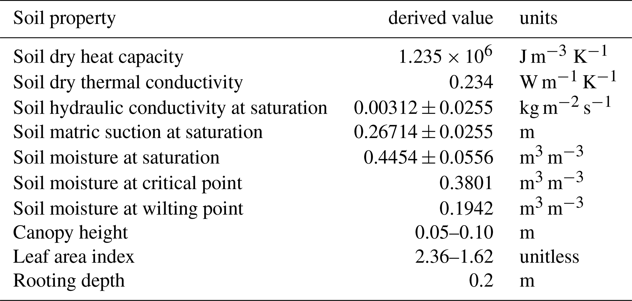
Figure 5 shows an example of observations and JULES output diagnostics over ten days in the summer of 2024 when the 2 m latent flux is available in addition to that at the standard 10 m height. The sensible and latent heat fluxes in Fig. 5 are uncorrected and taken directly from the archived files, i.e. the Bowen ratio method (Twine et al., 2000) of adjusting the fluxes to achieve energy balance has not been applied here. The basic configuration of JULES here is the MetUM-JULES Regional Atmosphere and Land configuration as described in Bush et al. (2025), albeit with the parameters modified according to Table 4. The period is dry apart from 18 mm of rainfall over a period of 12 h between 15–16 July. The effects of the rain can be seen in the increases in soil water content observed at 2, 10 and 22 cm and likewise in the simulated soil water. Although soil water observed (and modelled) at 57 cm depth (not shown) did not register any response to the rain, it is interesting that the water table shows a small rise at the end of 15 July (presumably responding to rain in the local area and therefore demonstrating local vertical soil water flow e.g. due to soil cracks) before decreasing over the remainder of the period. There is an increase in the daytime latent heat flux as observed at 2 and 10 m in the largely cloud-free days immediately after the rain as evapotranspiration strengthens. Although some of the highest observed latent heat values are not captured by the model (19 July at 10 m), some other flux data are well matched (17 July for both latent and sensible heat at 10 m). That being said, the JULES latent heat flux is in general well simulated at 10 m, although it is too large around midday at the 2 m height. This suggests that the near-surface gradients in the heat flux vertical profiles are not large enough in the model. So, although the peak values of the JULES 25 and 50 m sensible heat fluxes are suppressed, the sensible heat in JULES are overall close to the observations at 10 m. This is understandable if we look at the simulated skin temperatures that tend to be too warm in the middle of day (and too warm at night). Details aside, the change in Bowen ratio from the days immediately after rain (17–18 July) that have a Bowen ratio < 1, to the last day shown (24 July) when the ratio is > 1, is captured by the model.

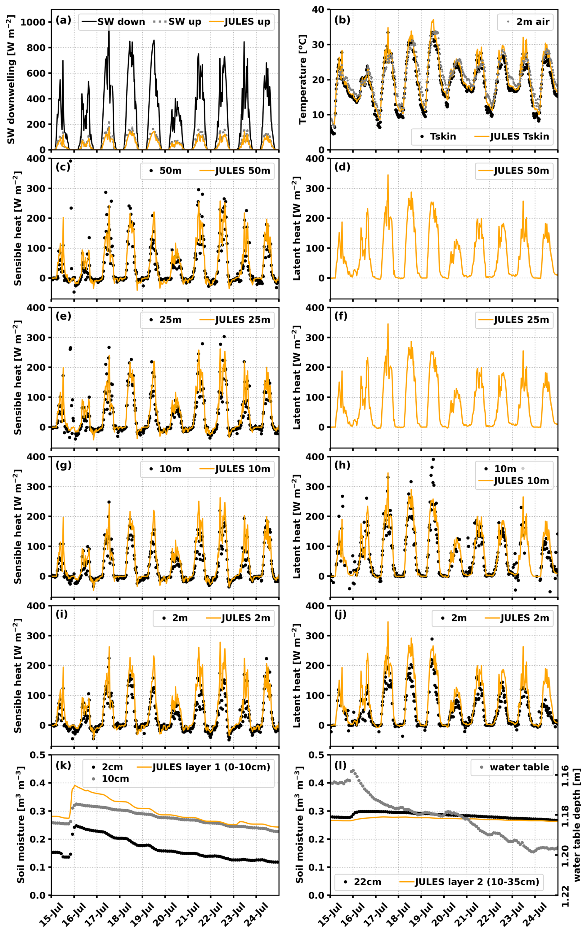
Figure 5 Comparison of JULES model output (yellow) and Cardington observations (black and grey dots) over ten days in July 2024. JULES has been forced using site data for 50, 25, 10 and 2 m with 30 min time steps. (a) Observed SW downwelling shows periods of cloudy and predominantly cloud-free conditions. (b) Skin (grass) and air temperatures, (c, e, g, i) sensible and (d, f, h, j) latent heat fluxes at the available heights, and soil moisture content at (k) level 1 and (l) level 2 are shown. The observed water depth is also included in (l) but this does not have a simulated equivalent.

5 Non-core remote sensing instruments

Figure 6 shows the data presence of the Halo Doppler lidars, ceilometers and microwave radiometers. Unlike Fig. 2 that shows availability after a basic level of quality control, the non-core data in Fig. 6 does not adhere to the same flagging system and so it only shows presence or not. Table 5 lists the various large devices by manufacturer that were operational at the site. Figure 6 shows fairly comprehensive data coverage for the ceilometers and the microwave radiometers (thanks to the reliability in particular of the WVR-1100). Doppler lidar data coverage was also substantial once they were installed in 2009 These more specialist instruments were not logged and processed centrally like the core dataset. Therefore, the core flagging method was not used for the non-core data in this section, and neither was it used for the radiosondes described later in Sect. 6. The various ceilometers were standard unmodified lidars ordinarily used on the Met Office operational network to detect cloud base height, but they also provide attenuated backscatter coefficient profiles from aerosol, precipitation and thin cloud. The other non-core dataset instruments are described in more detail below. Tables S6–S14 tabulate the variables and date/time structure in the archived non-core NetCDF files.

Table 5 Non-core remote sensing instruments (logged individually). The time interval represents both the logging rate and the archived time step. DBS = Doppler beam scanning, VAD = velocity azimuth display, LWP = liquid water path, IWV = integrated water vapour. NA: not available.

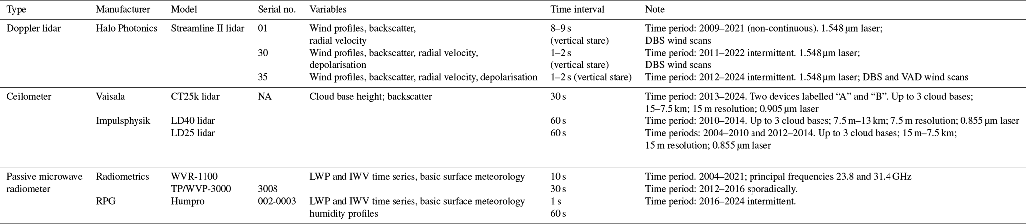
Figure 6 Data presence for individual, non-core remote sensing instrumentation. The three Halo Doppler lidars are in red, the three ceilometers are in blue, and the three microwave radiometers are in orange. Data from the j(NO₂) instrument in brown is contained within the core dataset files, not separately like the other instruments included here.

5.1 Halo Doppler lidars

Three Halo Photonics Streamline doppler lidars (Pearson et al., 2009) have been deployed at various times at the site. Table 6 summarises the Halo specifications for the three models operated at Cardington. Daily NetCDF files have been archived for each unit; Tables S8.1 and S8.2 list all the variables based on the radial backscatter data and wind profiles, respectively. Halo lidars are based on a 1.548 µm laser emitting linearly polarized pulsed light through an 8 cm diameter lens with a heterodyne detector. Laser beam returns from the atmosphere are range-gated velocity and back scattered power. The laser beam divergence from the lens was 33 µrad. Most of the beam returns are a result of aerosol particles acting as targets where the scattered light intensity and frequency shift are used to determine the attenuated backscattering coefficient and radial air velocity. Multiple pulses are averaged over a time interval called a ray. The Halo is capable of full hemispheric scanning of the backscatter coefficient and radial velocity as a function of beam range. The Halo laser interacts with relatively large aerosol particles compared to typical ceilometers (≈900 nm) and aerosol lidars (typically 355 or 532 nm) having shorter wavelength lasers. This often restricts the Halo instruments to boundary layer measurements (typically 1–3 km) because the free troposphere is typically very low in coarse mode aerosol concentrations, apart from sporadic elevated plumes such as those containing volcanic ash and mineral dust. Turbulent mixing, growth of diurnal boundary layers, development of the profiles of morning and evening transitions, nocturnal low-level jets, sea breeze fronts and other phenomena can all be observed with the Halo.

The radial velocity data during vertical stares can be used statistically over sufficiently long averaging intervals (10–60 min depending on the signal-to-noise ratio) to compute variance, skewness and kurtosis throughout the boundary layer and some distance into cloud (2–4 gates) before attenuation becomes significant. Therefore, quantities derived from the vertical velocity and backscatter coefficient – diagnosing updraughts and downdraughts, times of crossover and onset (Brooke et al., 2023) up to and including cloud base, and diagnosing boundary-layer type (Harvey et al., 2013) – can be determined.

Table 6 Halo Photonics Doppler lidar specifications.

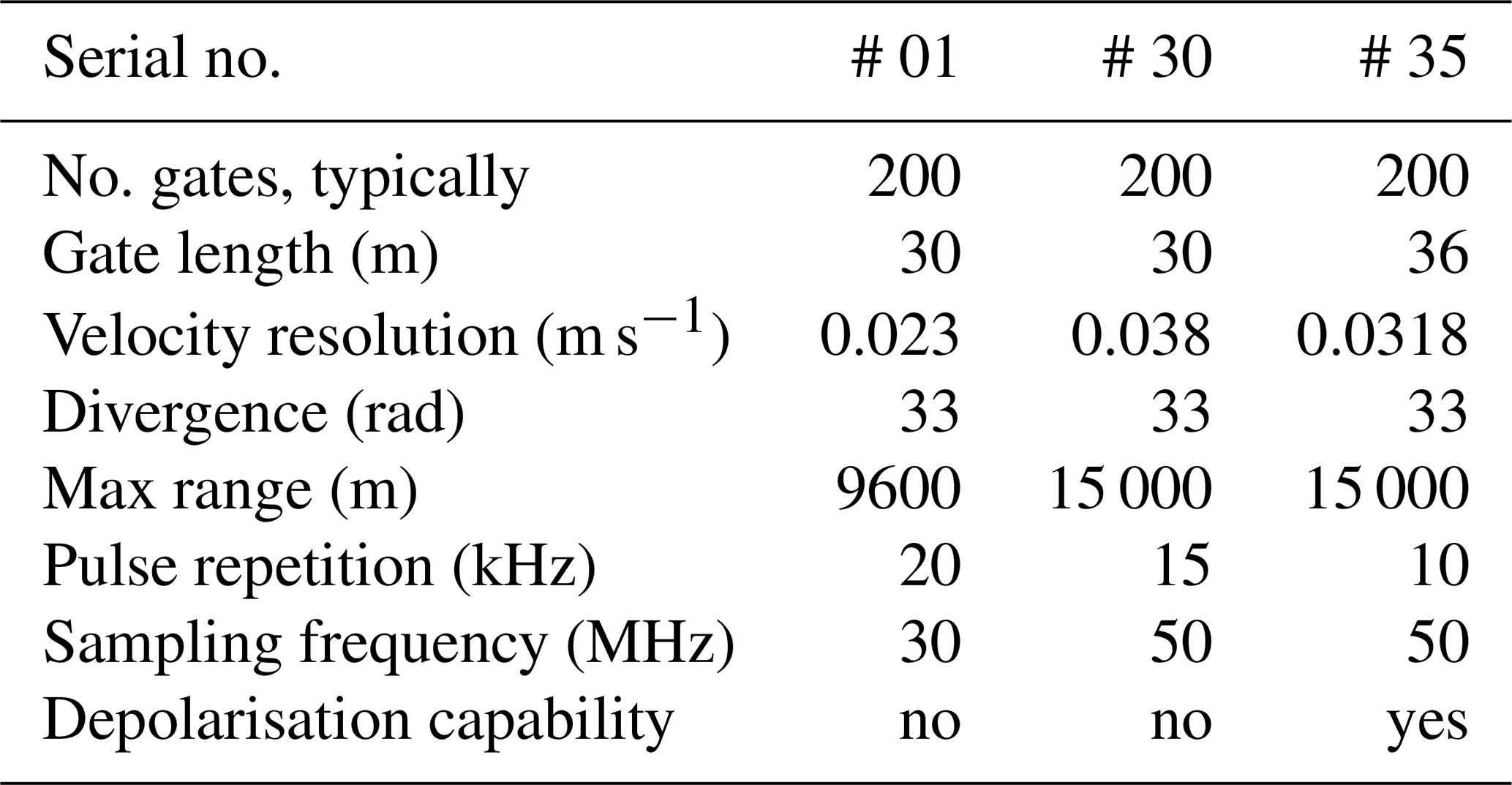
The usual operation at Cardington was vertical stares (zenith angle = 0°) with periodic wind scans that invoke various options of off-axis views. The vertical stares allow a near-continuous visualisation of the boundary layer from backscatter and vertical velocity. The raw data from either the vertical stares or off-axis scans was filtered according to a minimum signal-to-noise ratio of 0.01 (−20 dB) as standard. Although this threshold is higher than has been used by others (e.g. 0.0032–0.0045, or −25 to −24 dB, according to Vakkari et al. (2021)), it provides a consistent and reliable derivation of both vertical velocity and horizontal wind profiles. A signal-to-noise cut-off of 0.01 equates to an instrumental precision of around 1 m s⁻¹. Studies show that biases in the horizontal wind speed and direction amount to up to 7 cm s⁻¹ and 1°, respectively, with standard deviation uncertainties of 0.4−0.9 m s⁻¹ and 5–12°, respectively, compared to tower data up to 300 m (Newsom et al., 2017). For vertical velocities from the vertical stares, errors are expected to be always < 40 cm s⁻¹ and more like 3–4 cm s⁻¹ for high (>−10 dB) signal-to-noise ratios (Pearson et al., 2009). The first three gates of the Halo lidar are always unreliable due to crossover between the outgoing and return beams, i.e. 90–108 m above ground height depending on the prescribed gate length (Table 6). Angular precision of the optical scanner is ±0.05°.

Wind profiles performed every 30 min was the default operation for wind scans, although this was not strictly always the case. Most profiles of horizontal wind within the historical dataset are based on doppler beam swinging (DBS) scans which use a tri-axis azimuthally orthogonal technique using the single lidar beam to retrieve horizontal mean wind components. This scan was chosen for the bulk of the time because it only takes about 21 s to complete, which leaves 98 % of the available time to vertical stares if one wind scan is completed every 30 min. More recent scans have however used multi-axis velocity azimuth display (VAD) scans, which are effectively a more involved version of the DBS scans and use 6 or 12 point off-zenith views. Whatever the method employed, there is the assumption of a horizontally homogeneous wind flow and constant vertical velocity over the sampling volume, i.e. the volume defined by the conical “chunky slice” defined by the geometry of the lidar beam divergence and gate length. The two scan methods used to estimate vertical profiles of the horizontal wind speed and directions are described in more detail below. A third, rarely used type of scan was the range height indicator (RHI) where the elevation angle is stepped for a fixed azimuth angle. The vertical stares, DBS, VAD and RHI data are stored in separate archived NetCDF file names, as listed in Sect. 8. The scan files contain the same variables as the vertical stare files i.e. range, radial Doppler velocity, backscatter, signal-to-noise ratio for each of the scan positions. Derived profiles of horizontal wind speed and direction are stored in separate files as described in Sect. 8.

In Doppler lidar scanning, the measurement principle of radial velocity (v_r) is estimated from a probe volume using:

$$\begin{array}{}\text{(1)}& v_{\mathrm{r}}=\sin \mathit{\varphi }(u\sin \mathit{\theta }+v\cos \mathit{\theta })+w\cos \mathit{\varphi }\end{array}$$

where ϕ is the zenith angle (vertical = 0°) and θ is the azimuth angle (north = 0°), and u, v and w are the two horizontal components and vertical component of the wind field, respectively. During DBS scans, the measured vertical velocity component (v_z) from a vertical stare and two orthogonal off-zenith radial velocities (i.e. north-tilted v_n, and east-tilted v_e) at a fixed zenith angle ϕ (commonly 15°) allow the measured radial velocities to be derived from Eq. (1) as:

$$\begin{array}{}\text{(2)}& {\displaystyle }{v}_{\mathrm{n}}=v\sin \mathit{\varphi }+w\cos \mathit{\varphi }\text{(3)}& {\displaystyle }{v}_{\mathrm{e}}=u\sin \mathit{\varphi }+w\cos \mathit{\varphi }\end{array}$$

meaning we can then calculate the two horizontal wind components (u,v), alongside the vertical wind component w=v_z, thus:

$$\begin{array}{}\text{(4)}& {\displaystyle }u={\displaystyle \frac{v_{\mathrm{e}}-v_z\cos \mathit{\varphi }}{\sin \mathit{\varphi }}}\text{(5)}& {\displaystyle }v={\displaystyle \frac{v_{\mathrm{n}}-v_z\cos \mathit{\varphi }}{\sin \mathit{\varphi }}}\end{array}$$

which allows the mean vector wind speed ($\sqrt{u^{\mathrm{2}}+v^{\mathrm{2}}}$) and direction $\left({\tan }^{-\mathrm{1}}\frac{u}{v}\right)$ to be calculated.

DBS can be seen as a simplified version of velocity azimuth display (VAD) large-volume scanning and quicker to achieve operationally. VAD scans are nonetheless sometimes desired, e.g. an alternating combination of VAD and DBS scans might be carried out within certain study periods. With the more complex VAD scans, the geometric coordinate matrix containing the relationship between the radial velocities and the wind vector components is derived from Eq. (1) and takes the form of A= [sinϕ sinθ, sinϕ cosθ, cosϕ] for the specified number of azimuth and zenith angles. This is usually over an azimuthal scan of either 6 or 12 points for a fixed zenith angle (15° from vertical, for example). A least squares approximation is then sought as the solution to the linear vector matrix equation $\mathbf{A}\cdot \mathit{v}={\mathit{v}}_r$ (that has no absolute solution), where v_r is the vector of the measured radial velocities for the separate beams and v is the 3-dimensional wind vector containing the u, v and w components we require, such that v= (A^TA)⁻¹ A^T v_r, with A^T indicating the transposed matrix. The mean wind speed and direction can then be calculated from the derived components.

The linear depolarisation ratio (Vakkari et al., 2021) was also possible with Halo30 and Halo35, although this was not switched on by default. The co- and cross-components of the returned laser pulses from non-spherical aerosol particles or ice crystals was achieved with a fibre-optic switching polarizer. Depolarisation ratio as a function of zenith angle of orientated ice crystals in cirrus clouds (such as used in Westbrook et al., 2010) has been studied to some degree using Halo35 data, although this technique was not fully developed because the scanning had to be done manually and was not able at the time to be automated using the available control software. The cross-component data gathered at Cardington is nonetheless included as separate archive files (see Sect. 8).

5.2 Microwave radiometers

The passive microwave radiometers at Cardington allowed continuous monitoring of integrated water vapour, liquid water and sometimes profiles of humidity and temperature. Microwave radiometers utilise emission lines in the incoherent absorption microwave band exhibited by gaseous and liquid water. Various types of internal and external calibrations are required for these radiometers due to the huge gains (usually 60–80 dB) required to do the retrievals. Three models of radiometer that were deployed at Cardington are described below, all of which used zenith views for the retrievals with periodic off-zenith views for calibration purposes. Retrievals of humidity have inherently larger errors relative to temperature because (i) microwave sensitivity is weaker for water vapour, (ii) humidity signals are more affected by cloud water and precipitation, with the retrieval accuracy degrading with cloud depth, and (iii) the neural networks that have been used in profile retrievals of humidity can especially struggle with the high variability of humidity in the boundary layer alongside larger error in humidity measurement from radiosondes used in neural network training (Zhang et al., 2024). The neural networks used for all retrievals here were traditional multilayer backpropagation methods. Although it is appreciated that more robust deep learning methods using increased hidden layers are now available that can reduce errors – e.g. Yan et al. (2020) show that RMS errors for retrievals of RH, absolute humidity and air temperature can be reduced using deep learning from 15 % to 11 %, 0.44 to 0.26 g m⁻³, and 3.3 to 1.7 °C, respectively, based on profiles of the whole troposphere – it is beyond the scope of the Cardington dataset to apply such methods to the processing.

The Radiometrics Corporation WVR-1100 passive radiometer (Wang et al., 2017) was the longest serving such device and measured the atmospheric emissions at two frequencies, 23.8 GHz K-band and 31.4 GHz Ka-band, which provide brightness temperature at these channels (with RMS error of 0.3 K) and thereby information of the column water vapour and liquid water. No humidity or temperature retrievals were performed with the WVR-1100. The WVR-1100 used a bi-linear regression method based on local radiosonde launches to retrieve column integrations of liquid water and water vapour (Price, 2003). A large number of past radiosonde launches were required that had been carried out from the site at which the radiometer was located; concurrent launches are not required in general in order to operate microwave radiometers. Although the WVR-1100 performed “tipping curve” observations using off-zenith scans where optical depth varies in a known way with atmospheric geometrical thickness, this data was in effect only used for calibration purposes and is not stored in the archived files. The overall error in liquid water path is estimated to be ±0.015 kg m⁻² (or ±0.0015 cm of precipitable water) in non-precipitating non-glaciated clouds. RMS error in the water vapour column is estimated as within 0.5 kg m⁻² (or 0.05 cm of precipitable water). Water vapour and liquid water column amounts were logged typically every 9–10 s. As with all microwave radiometers, absolute calibrations for the absorbing channels were done occasionally (such as when the radiometer was moved) using an external black body cooled with liquid nitrogen. See Table S9 for full list of variables for the WVR-1100.

The Radiometrics TP/WVP-3000 microwave radiometer (Ware et al., 2003) was mostly used on detached duty and therefore relatively little at Cardington; we nonetheless still include the available data in the archive. The TP/WVP-3000 observed radiation at 12 frequencies (22.035, 22.235, 23.835, 26.235, 30.0, 51.25, 52.28, 53.85, 54.94, 56.66, 57.29, and 58.8 GHz) containing various water and oxygen emissions. RMS error in the brightness temperatures is within 0.5 K (Ware et al., 2003) and differences to radiosonde profiles show a standard deviation in the water vapour column of 0.8 kg m⁻² (Gaffard and Hewison, 2003). Liquid water path uncertainties decrease from 20 % for LWP > 0.1 kg m⁻², to 50 % for LWP ∼ 0.05 kg m⁻², to 100 % for optically thin clouds of LWP ∼0.01 kg m⁻². Both the TP/WVP-3000 and the RPG Humpro described below used a neural network to retrieve profiles of water temperature and water vapour (both absolute and relative humidities are calculated). The neural network was trained with a radiative transfer model using multiple years of radiosonde data. Typical RMS errors for temperature, RH and absolute humidity profile retrievals are 2 °C, 20 % and 0.44 g m⁻³, respectively (Gaffard and Hewison, 2003). The TP/WVP-3000 was set up to take readings in the vertical approximately every 8 s. Regular tipping curve scans in the K-band were done over a range of zenith angles (30, 45, 90, 135, 150°) to compare the atmospheric radiances to that of known values at relatively opaque water vapour frequencies (with the opacity being a linear function of the slant path), in addition using frequent views of an internal temperature-controlled black body. However, as with the WVR-1100 tipping curves, none of the off-axis data is stored in the processed files. See Table S10 for full list of variables for the TP/WVP-3000. All retrieved variables, whether profiles or column time series, are stored in the same daily NetCDF files.

The RPG Humpro profiling radiometer retrieved absolute and relative humidity profiles in addition to the usual liquid water and integrated water vapour paths using brightness temperatures measured at seven microwave frequencies at 22.24, 23.04, 23.84, 25.44, 26.24, 27.84 and 31.4 GHz. Although the K-band noise was typically ∼0.1 K, the drift between calibrations could be 0.4 K. Water vapour column and LWP are retrievable with RMS errors of 0.2 and 0.05 kg m⁻², respectively. RMS errors of absolute humidity profiles retrieved with the Humpro have been shown to be typically 0.33 g m⁻³, or 15 % in terms of RH, and the RMS error for temperature in the boundary layer, where accuracy is relatively high, was about 1.9 °C (Debnath, 2020). The Humpro has variable resolution in the vertical i.e. 200 m between 0−2 km, 400 m for 2–5 km, and 800 m for 5–10 km. Two archive files were produced, based around the time series (water vapour and LWP) and profile (humidity) data. See Tables S11.1 and S11.2 for the full list of time series and profile variables, respectively.

5.3 Ceilometers

The three models of near-infrared diode laser ceilometers, which are simple backscatter lidars used operationally, installed at Cardington (called the LD25, LD40 and CT25K as shown in Table 8) are able to retrieve not only cloud base height (at up to three levels if penetration power is sufficient), but also cloud penetration depth per cloud layer, the vertical visibility, and a measure of the vertical profiles of backscattered intensity in a similar manner to the Halo Doppler lidars. There were two CT25K ceilometers installed, with the second unit deployed from October 2015 and is called CT25K_B in the archived NetCDF files. The CT25K_B was tilted 4° from the zenith to avoid specular backscatter from cirrus clouds. The other ceilometers all pointed in the true zenith. For the cloud-base height retrievals from the CT25K_B, the height above ground level was corrected for the instrument tilt. Table S12 lists the variables in the ceilometer NetCDF files.

5.4 Radar Wind Profiler

The National Centre for Atmospheric Science (NCAS) mobile Degreane Horizon PCL1300 Radar Wind Profiler (RWP) owned by the University of Manchester was originally purchased by Aberystwyth University in 2002. The RWP was deployed at Cardington for non-continuous periods between 2002 and 2016 as part of collaborative work with the Met Office. The advantage of the RWP over a lidar is that it can measure in and above cloud. Technically a L-band radar operating at 1290 MHz, these RWPs are commonly called UHF Doppler radars in the literature. At this frequency radars detect clear air echoes from variations in refractive index on a scale of 23 cm. In the lower atmosphere these irregularities are mainly due to humidity fluctuations. In the presence of hydrometeors stronger Rayleigh scattering dominates the signal.

The RWP consists of three static arrays of dipole antennae panels that both emit and receive three separate beams. The vertical panel measures the vertical component of the wind, and the other panels at elevations of 73° and orthogonal azimuths provide a direct measurement of the mean radial velocity along the radar beam. The RWP cycles between the antenna directions and data is combined to calculate full wind vectors. The RWP measures wind speed (direction) to an intrinsic accuracy of < 1 m s⁻¹ (<10°) in all weather conditions. In principle, the minimum altitude was 75 m depending on ground clutter signals and atmospheric conditions with a minimum vertical gate spacing of 75 m. The radar typically returned wind profiles from around 75 to 4500 m depending on atmospheric conditions.

Data is archived as daily NetCDF files (detailed in Table S14) using 15 minute averages and can be found at the CEDA repository, albeit not as part of the Cardington archive otherwise described in this paper. Applications of RWP data can be found in Norton et al. (2006), Morcrette et al. (2006), Parton et al. (2009) and Osborne and Lapworth (2017).

6 Radiosonde archive

We include the historical archive of radiosonde launches at Cardington going back to 1996. Although this goes back seven years more than the surface site core dataset archive, this was relatively straightforward to do due the consistency in data format. There were a large number of routine daily or twice-daily launches during 1997 and especially 1998 that have the potential to be used statistically by future data users. Examples from the past of using large numbers of radiosonde soundings for instrument validation include microwave radiometer retrievals (Price, 2003; Gaffard and Hewison, 2003) and lidar profiling of water vapour (Gaffard et al., 2021).

Table 7 summarises the major Vaisala sonde package types and associated generation of the ground receiving station. Figure 7 displays in the top panel the number count of launches as a function of date, coloured by campaign year. The same colours are used in the bottom two panels showing histograms of the hourly time of launch and sounding termination height. The termination height was determined by setting a timer during the sonde initialisation, or terminating the sonde manually during flight, or when the balloon bursts naturally at altitude. Additionally, sometimes an increase in pressure, and therefore a decrease in sonde altitude, would cause the software to terminate the sounding.

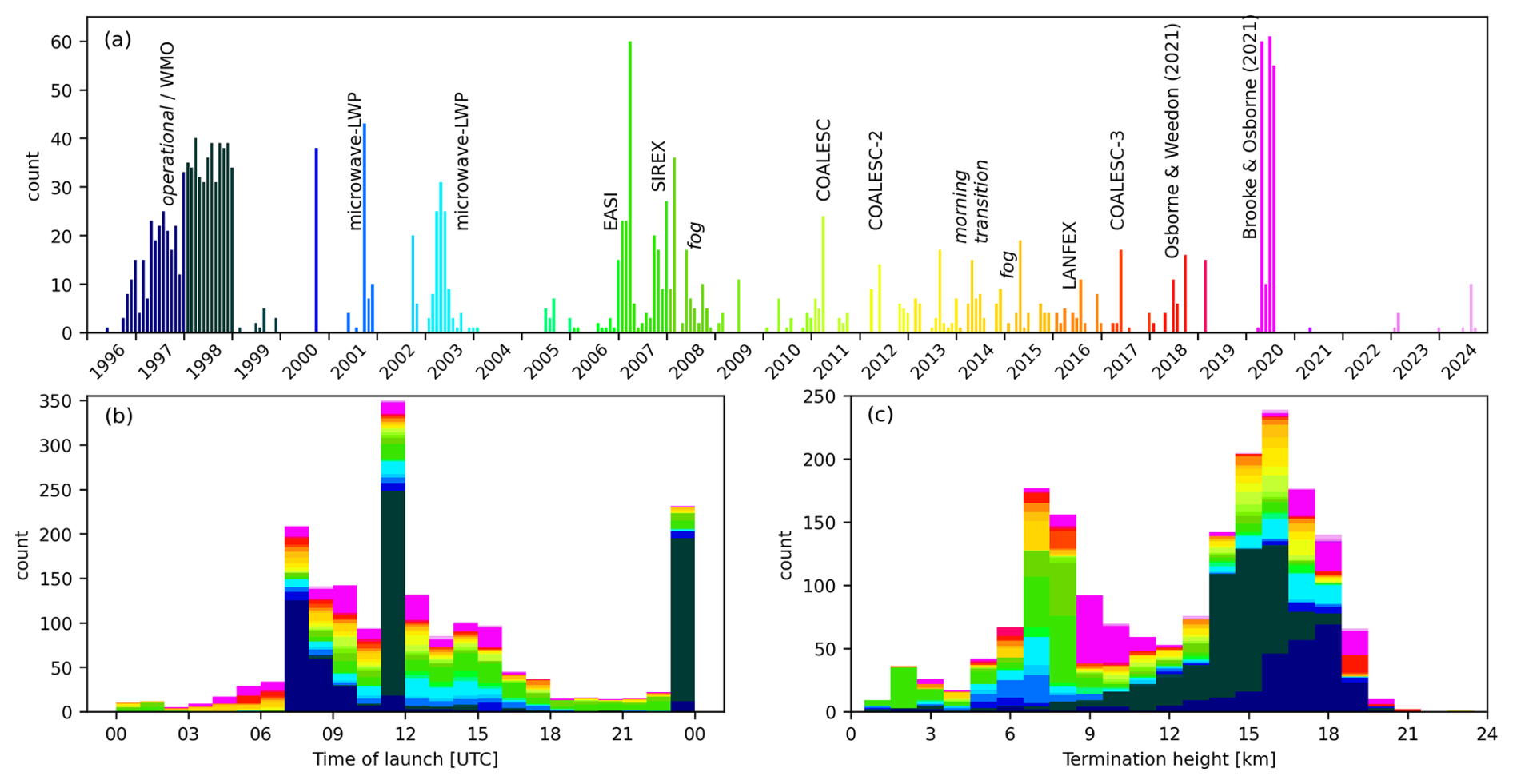
Figure 7 Summary of radiosonde launches at Cardington: (a) Number of launches per month with annotations of significant campaigns – colours are used to distinguish years in the manner as the next two panels, (b) histogram of time of launch with 1-hourly bins, (c) histogram of sonde termination height with 1 km bins. COALESC = Combined Observations of the Atmospheric boundary-Layer to study Evolution of StratoCumulus; EASI = East Anglia Stratocumulus Investigation; LANFEX = Local and Non-local Fog Experiment; SIREX = Surface Inhomogeneity Research Experiment; WMO = World Meteorological Organization database.

Figure 7 shows the largely sporadic nature of radiosonde launches at Cardington, which shows how launches were focussed on campaigns with distinct research goals (as annotated by research type or campaign name) that would vary the time and frequency of launches. A notable exception was in 1997 and 1998 where launches were carried out daily (sometimes early morning but mostly at midday and midnight) for an extended period. The lack of sonde launches between 2021 and 2023 was because of detached campaigns which meant the focus was away from Cardington. Launches not annotated in Fig. 7 were opportunistic launches based on interesting weather events (e.g. thick fog) or at the request of operational forecasters in the Met Office who wanted to understand the structure of the atmosphere better during periods of troublesome weather conditions.

Table 7 Summary of radiosonde and receiving station versions.

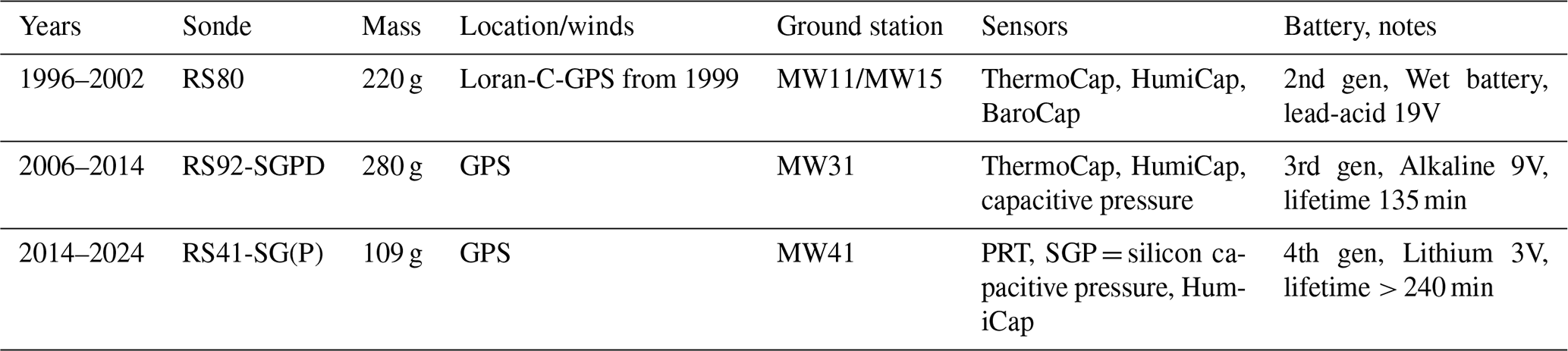
The majority of sonde launches at Cardington were performed with small 100 g latex balloons that were filled with enough helium to provide a mean ascent rate of 2.5 m s⁻¹. This is about half the rate of the operational Met Office launches, for example, that use 700 g balloons. The slower ascent rate was used to improve the vertical sampling resolution in the atmospheric boundary layer whilst maintaining a sufficient ventilation rate over the sensors. Because almost all of research at Cardington concerned the boundary layer, many sonde launches were terminated at low altitude so that rapid-fire launches could be carried out (e.g. 30–45 min intervals between launches during fog research).

During the ground preparation of each sonde unit the humicap and PRT sensors were heated to 150 °C to remove contaminants, a procedure called conditioning, then zero humidity and in-built temperature checks were performed. A ground truth for the pressure sensor is also entered and once a stable pressure reading is secured, and the sensor boom has cooled down, then the sonde is ready for launch. Unless a fault with one or more of the sonde variables was noted during flight, with the possibility of terminating the sonde and launching another to replace it, no routine quality control was carried out on the data in the sonde archive. Each launch sounding has its own NetCDF file and the Table S13 lists the variables in full.

7 Data availability

All data described in this paper is stored on the UK-based CEDA repository (https://archive.ceda.ac.uk, last access: 24 February 2026) as NetCDFs, all of which comply to the CF-1.8 ACDD-1.3 conventions. The Dataset Collection for Met Office Meteorological Research Unit, Cardington is publicly available at https://doi.org/10.5285/5487380511084413a502c4b229273bc6 (Met Office et al., 2025).

Use of these data is covered by the licence at https://www.nationalarchives.gov.uk/doc/open-government-licence/version/3/ (last access: 20 February 2026). When using these data, you must cite them correctly using the citation given on the CEDA Data Catalogue record. Separate DOIs are provided for each of the datasets outlined above, i.e. at the four different time steps of the core dataset, with the large radiometers, radiosondes and derived LSM forcing files supplied with separate links. All data are divided into daily files, except for the LSM forcing files (necessarily continuous at 30 min time intervals from 2005 to 2024) and the radiosondes (one file per launch).

8 Summary

Well instrumented meteorological sites are important for the development and testing of land surface models. This paper describes the 20-year (2004–2024) Met Office ground-based surface and near-surface meteorological and subsoil hydrological dataset from Cardington in central England. The variables that encompass atmospheric turbulence fluxes over a range of heights and the components of the near-surface energy balance, together with subsoil temperature and moisture sensors that include water table depth, make the dataset relatively unusual and potentially useful for both model evaluation and development of LSMs. Meteorological records of evapotranspiration and CO₂ fluxes using the eddy covariance method having a continuous duration of 20 years or more, as shown here in the Cardington dataset, are scarce (Li et al., 2025).

The Cardington core dataset has been quality controlled and is archived with open-access at the UK CEDA repository. This core data consist of four daily NetCDF files based on four averaging periods (1, 5, 10 and 30 min). Use of the open-access data is subject to referencing this paper and acknowledgement of the CEDA repository. A subset of the core dataset has been used to generate four forcing files suitable for driving LSMs at a 30 min time step. These files represent the whole 20-year period for the three main drive heights, i.e. 10, 25 and 50 m, plus the 2 m level from 2012 i.e. only whole years are included in the forcing files. The soil properties of the site were summarised in Table 7, which allows users to configure their simulations to local conditions. Specialist Doppler lidars, ceilometers, precipitation disdrometer and microwave radiometers are in addition archived into daily NetCDF files based on the averaging interval as set for each instrument. Finally, there are the sporadic radiosonde soundings that are also archived, with one NetCDF file per radiosonde launch. These amount to around 1800 site launches since 1996.

Use of the Cardington data in the past has tended to focus on shorter time periods of between the order of a day up to a few months. Decadal analysis of soil conditions and turbulence characteristics, for example, remain untapped. Similarly the Licor CO₂ data are yet to be used. We showed an illustration of the momentum roughness length trends at various mast heights in Fig. 4. The roughness length was shown to vary with measurement height and with time, averaged over both winter and summer seasons, as land use changed. Further analysis could break the data down into further wind sectors as we only used data from the prevailing 155–280° sector. We hope this, alongside the snapshot of turbulent heat flux and soil data in Fig. 5, serves as an advertisement for others to use the available data.

Another aspect not addressed directly was instruments that measured similar or related variables with overlapping time periods that could allow biases to be quantified and potential instrument corrections to be applied. Examples include (i) use of radiosonde boundary layer wind profiles to compare to the UHF wind profiler and Halo Doppler lidar; (ii) use of radiosonde profiles in further microwave radiometer humidity retrieval trials, (iii) in-situ humidity measurement from multiple sensors (humicaps, chilled-mirror and high-speed optical hygrometers), (iv) use of the two heat flux plates and soil temperature and moisture sensors to assess and correct the ground heat flux in a rigorous manner for its use in energy balance studies.