Environment90m – globally standardized environmental variables for freshwater science at high spatial resolution

The current loss of freshwater biodiversity calls for immediate action, including the mobilisation of existing data and tools to support long-term conservation. Yet, establishing a global baseline for the spatial distribution of freshwater habitats and the biodiversity they host remains difficult. Such task would require standardized, high-resolution environmental information to characterise freshwater habitats anywhere in the world. To address this challenge, we present the Environment90m dataset, which aggregates a large number of environmental layers into each of the 726 million sub-catchments of the Hydrography90m dataset, corresponding to single stream segments. Specifically, Environment90m includes 45 variables related to topography and hydrography, 19 climate variables for the observation period of 1981–2010, as well as projections for 2041–2070 and 2071–2100 under the Shared Socioeconomic Pathways (SSPs) 1.26, 3.70 and 5.85, and three global circulation models (UKESM1-0-LL, MPI-ESM1-2-HR and IPSL-CM6A-LR). Moreover, Environment90m includes 22 land cover categories for the annual time-series data from 1992–2020. In addition, we provide 15 soil variables and information on aridity and modelled streamflow. Summary statistics (i.e., mean, min, max, range, sd) are provided for all continuous variables, while for categorical data, the proportion of each category is calculated within each of the sub-catchments. The data is available at https://hydrography.org/environment90m (last access: 4 February 2026). To facilitate data download and processing, we provide dedicated functions within the hydrographr R-package, and extend these also to new functions for processing upstream data of lakes. For all underlying calculations, we used the open-source tools GDAL/OGR, GRASS-GIS and AWK, so that custom data can be easily generated using the hydrographr R-package. Environment90m, along with the tools, provides an array of opportunities for research and application in spatial freshwater biodiversity science, specifically biogeographic analyses and conservation exercises in freshwater ecosystems. The metadata of the Environment90m dataset is stored at https://doi.org/10.18728/igb-fred-995.0 (García Márquez et al., 2025a).

1 Introduction

Freshwater ecosystems and biodiversity are considered to be more threatened than their terrestrial and marine counterparts (WWF, 2020; Tickner et al., 2020). Advances towards the protection of freshwater habitats remain elusive, despite recent efforts to secure their long-term protection. Examples include the so-called “30-by-30” protection target, which aims to protect 30 % of Earth’s lands, oceans, coastal areas and inland waters (The Post-2020 Global Biodiversity Framework, Hughes, 2023). In addition, the recent EU Nature Restoration Law also aims to restore river connectivity (Stoffers et al., 2024). In the context of these political initiatives, large-scale standardized analyses on the spatial, environmental and biotic characterization of freshwater habitats and their connectivity are required to, e.g., answer the question: “which areas should be prioritized for protection?”. Addressing this question requires at minimum a detailed baseline of the present-day spatial distribution of the environmental characteristics of freshwater habitats. Only after establishing a baseline, the environmental changes, or changes in biodiversity can be measured and quantified. Such knowledge allows to assess freshwater biodiversity using, e.g., species distribution modelling techniques (Bellin et al., 2022). Likewise, it allows to also perform connectivity-related analyses to support the restoration of fragmented rivers (Hermoso, 2025).

In the freshwater realm, information on such environmental characteristics should ideally be available at very high spatial resolution. This is because (i) it can be attributed to the corresponding water body, e.g., a specific stream segment and (ii) environmental characteristics are not aggregated across large areas, avoiding issues related to the Modifiable Area Unit Problem (MAUP) (Jelinski and Wu, 1996). The MAUP is a statistical feature which occurs when data is aggregated to spatial units, whose size may influence the aggregated values (e.g., by using grid cells of varying size). In the freshwater realm, spatial units are more realistic when they correspond to drainages, larger sub-catchments or standing water bodies such as lakes. Therefore environmental information is commonly aggregated within these units. A key goal is thus to have environmental information at the highest possible spatial resolution, allowing to incorporate the crucial feature of longitudinal connectivity, while still achieving computational efficiency of workflows. The environmental conditions along the dendritic network structure can be depicted following various concepts: the River Continuum Concept (Vannote et al., 1980), macrosystem theory (Thorp, 2014) or functional process zones (Maasri et al., 2019). At the same time, tributary inputs, lateral connectivity with floodplains, and discontinuities caused by natural or anthropogenic disturbances also play a role in shaping the environmental conditions along the dendritic stream network (Ward and Stanford, 1983, 1995; Benda et al., 2004). To characterize this environmental continuum along the network requires, in turn, to pinpoint the relevant environmental conditions and processes to single network segments. Hence, the spatial aggregation of environmental information, which usually comes in gridded datasets at, e.g., 1 km spatial resolution, has to match the spatial configuration of the water bodies (Brunner et al., 2024; Friedrichs-Manthey et al., 2020). In this regard, sub-catchments which correspond to single stream segments are, unlike pixels, non-randomly distributed across the surface and follow the topographical and topological gradients in the landscape (Brunner et al., 2024).

Therefore, in freshwater systems, the sub-catchments of single stream segments can be considered as the smallest hydrological units. They have their own ecological and hydrological boundaries, encompassing the aquatic-terrestrial linkages (Linke et al., 2007). They also feature the same connectivity as the network, but also allow including the terrestrial landscape into the analysis workflow, which is of interest when performing biogeographic analyses of semi-aquatic organisms, such as aquatic insects, amphibians or mammals, which rely on both ecosystems.

Aggregating environmental variables across sub-catchments is often done on a case-by-case basis, while there are only few datasets that cover wide spatial gradients. A global extent is given by the HydroATLAS (Linke et al., 2019) and the HydroLAKES datasets (Messager et al., 2016; Lehner et al., 2022), as well as a near-global aggregation of upstream-catchment variables (Domisch et al., 2015) which follow the HydroSHEDS river network (Lehner et al., 2008). National efforts include the StreamCAT Dataset (Hill et al., 2016) and LakeCAT Dataset (Hill et al., 2018) which correspond to the high-resolution NHDPlusV2 river network in the United States (McKay et al., 2012).

In contrast to all previous examples, the Hydrography90m dataset (Amatulli et al., 2022), includes the most detailed stream network channel at 90 m spatial resolution. This global network incorporates for the first time headwater stream segments, that is, streams of 1st and 2nd Strahler order (Strahler, 1957). Although some estimates indicate that 70 % of global stream networks consist of 1st and 2nd order streams (Lowe and Likens, 2005; Leopold et al., 2020), they have been neglected so far in regional and global biodiversity assessments. Hydrography90m comprises 1.6 million drainage basins, 726 million stream segments and sub-catchments, along with 42 stream-topographical and -topological variables. Each sub-catchment corresponds to one stream segment, sharing a unique ID.

With this level of detail, aggregating environmental variables across sub-catchments implies computationally heavy calculations and data storage challenges. With the introduction of the Environment90m dataset, we expect to facilitate globally standardized analyses and modelling workflows by aggregating environmental variables at global scale and at high spatial resolution based on the Hydrography90m stream network (Amatulli et al., 2022). Environment90m includes 45 variables related to topography and hydrography, 19 climate variables for the observation period of 1981–2010, as well as projections for 2041–2070 and 2071–2100 under the Shared Socioeconomic Pathways (SSPs) 1.26, 3.70 and 5.85, and three global circulation models (UKESM, MPI and IPSL). Moreover, Environment90m includes 22 land cover categories for the annual time-series data from 1992 to 2020. In addition, we provide 15 soil variables and information on aridity and modelled stream flow. Summary statistics (i.e., mean, minimum, maximum, range, standard deviation) are provided for all continuous variables. For categorical variables, the proportion of each category is calculated within each sub-catchment. The current version of the Environment90m dataset is 4.1 terabytes (TB) in size. The data is available at https://hydrography.org/environment90m (last access: 4 February 2026) (see also Sect. 2.3).

To mobilize the Environment90m data integration into workflows, we provide two options: first, we have developed custom functions for batch downloading, processing and integrating the data with the Hydrography90m network, as well as for performing custom workflows, within the hydrographr R-package (Schürz et al., 2023). Second, all Environment90m aggregated variables are also available on the GeoFRESH online platform (available at https://geofresh.org/, last access: 4 February 2026, Domisch et al., 2024), which allows to quickly download the variables for point locations globally, both for the given sub-catchments where the points are located and their entire upstream catchments. Moreover, a new set of hydrographr functions allows to aggregate the data over lakes, as well as single river-lake intersections (Tomiczek et al., 2024). For example, users can retrieve the Environment90m information for each lake's upstream catchment area. We showcase the workflow in this exemplary lake vignette, available at https://glowabio.github.io/hydrographr/articles/case_study_lakes.html (last access: 4 February 2026).

2 Methods

2.1 Workflow for the development of the Environment90m dataset

The Environment90m dataset consists of tabular data including the summary statistics of 104 environmental variables from 7 different datasets, which we aggregated over each of the 726 million unique sub-catchments of the Hydrography90m dataset (Amatulli et al., 2022), yielding different summary statistics. The output tables are available in different formats (Fig. 1, and see also Sect. 2.3). We selected variables that are available continuously (i.e., range-wide) at the global scale with a resolution of 1 km or less, and which are widely used or can potentially be used to describe freshwater habitats and biodiversity distribution patterns. The following sections describe the original datasets and the processes we followed for their aggregation.

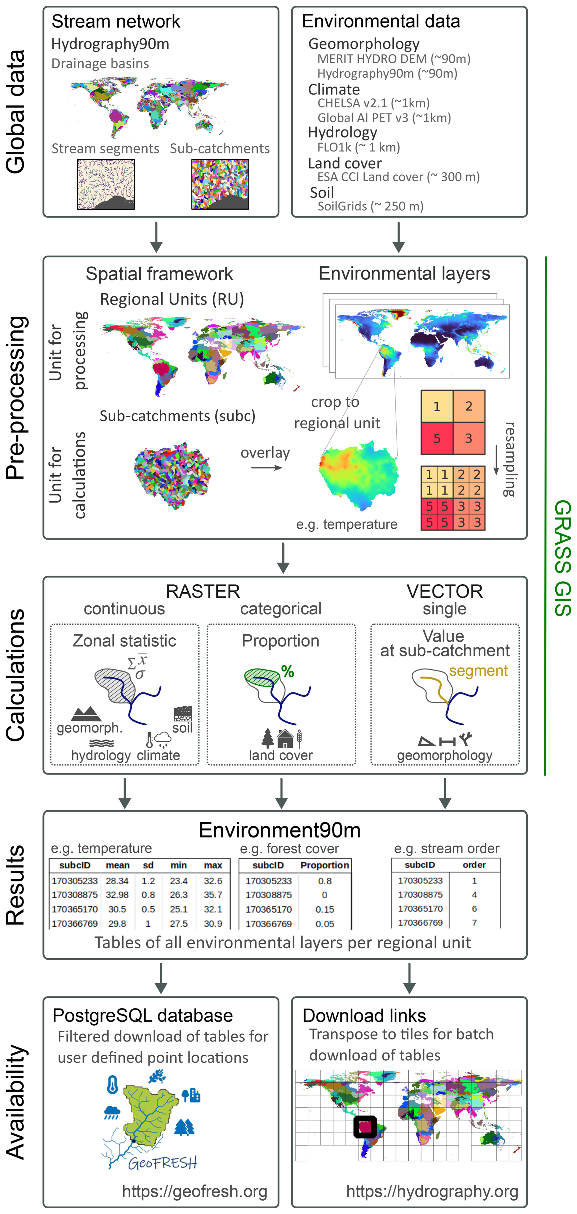
Figure 1 Workflow for the development of the Environment90m dataset. The process starts with the selection of environmental variables and their resampling to match the 90 m resolution of the Hydrography90m sub-catchment layer. The aggregation is done through several raster and vector calculations. The final tables are available to download at https://hydrography.org/environment90m/ (last access: 4 February 2026) and can be also queried in the GeoFRESH online platform at https://geofresh.org/ (last access: 4 February 2026).

We started the procedure by creating a working session in GRASS GIS (Neteler et al., 2012) for each of the 166 Regional Units (RUs) defined in Amatulli et al. (2022) (see also Fig. 7 therein). Regional units are groups of one large or several entire drainage basins, ensuring that the whole area of the sub-catchments belonging to a drainage basin is included in the RU. This design aims to improve the efficiency of computational calculations. The GRASS GIS session initialization was made with the raster file of each RU containing the sub-catchments, which automatically provided the geographical extent and the resolution (90 m) of the raster file as the default settings of the session. The default coordinate reference system was set to the World Geodetic System 1984 (WGS 84) with coordinates expressed as latitude and longitude, as defined by the EPSG:4236.

The raster files of the environmental variables were then read into each of the GRASS GIS sessions, where they were cropped and resampled to the same extent and resolution using the default settings. In all our cases, the original raster files had a resolution equal or lower than 90 m. In case the environmental layers had a lower resolution, as CHELSA climate at a 30 arcsec (1 km) resolution, their grid cells were resampled to 90 m without interpolation, i.e., all new 90 m cells were assigned the same value as 1 km cells if they overlapped (GRASS Development Team, 2024). This procedure is explained in Fig. 2.

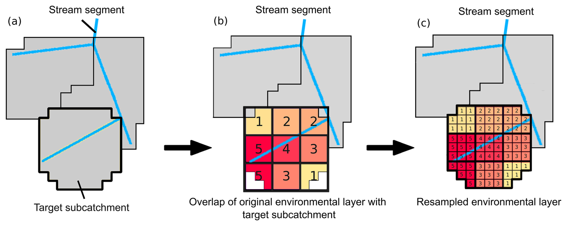
Figure 2 Resampling procedure (from lower to higher resolution) when reading environmental datasets into the default settings of a GRASS GIS session. (a) shows an example of different stream segments and their corresponding sub-catchments. The sub-catchment with the bold boundary is the target sub-catchment to illustrate the resampling procedure. (b) shows the overlap of the environmental data (originally with a lower resolution, e.g., 1 km) with the target sub-catchment. In (c) the original dataset is resampled to the 90 m resolution of the target sub-catchment, such that all new 90 m raster cells have the corresponding value as the lower resolution cell.

We selected between three possible methods to calculate summary statistics when creating the output tables, following the properties of each environmental dataset:

1. Zonal statistics. Calculation of the mean, standard deviation, range, minimum, and maximum of the environmental layer within each sub-catchment. Environmental layers with continuous values (e.g., temperature) fell into this category. The calculations were done within the GRASS GIS environment using the r.univar function.

2. Proportion. The proportion of the variable (i.e., variable categories) within each sub-catchment. Categorical data, namely land cover, belonged to this category. The calculations were done within the GRASS GIS environment by dividing the number of pixels of each land cover category in each sub-catchment by the total number of pixels in the sub-catchment.

3. Value at sub-catchment. Hydrography90m provides a vector file with a list of attributes for every stream segment globally. Since every sub-catchment shares a unique ID with each stream segment, the value assigned to the sub-catchment corresponds to the value of the different attributes in the stream segment vector file (Amatulli et al., 2022). Examples of these attributes include stream length or Strahler stream order (Strahler, 1957).

All calculations were performed in parallel using the High Performance Computing (HPC) facility at Yale University.

2.2 Description of the underlying environmental datasets

The following sections describe the underlying environmental datasets used to generate Environment90m. The tables refer to the properties of the original datasets. The exact abbreviations used in Tables 1–7 should be used to retrieve the variables from the Environment90m dataset.

2.2.1 Stream network data

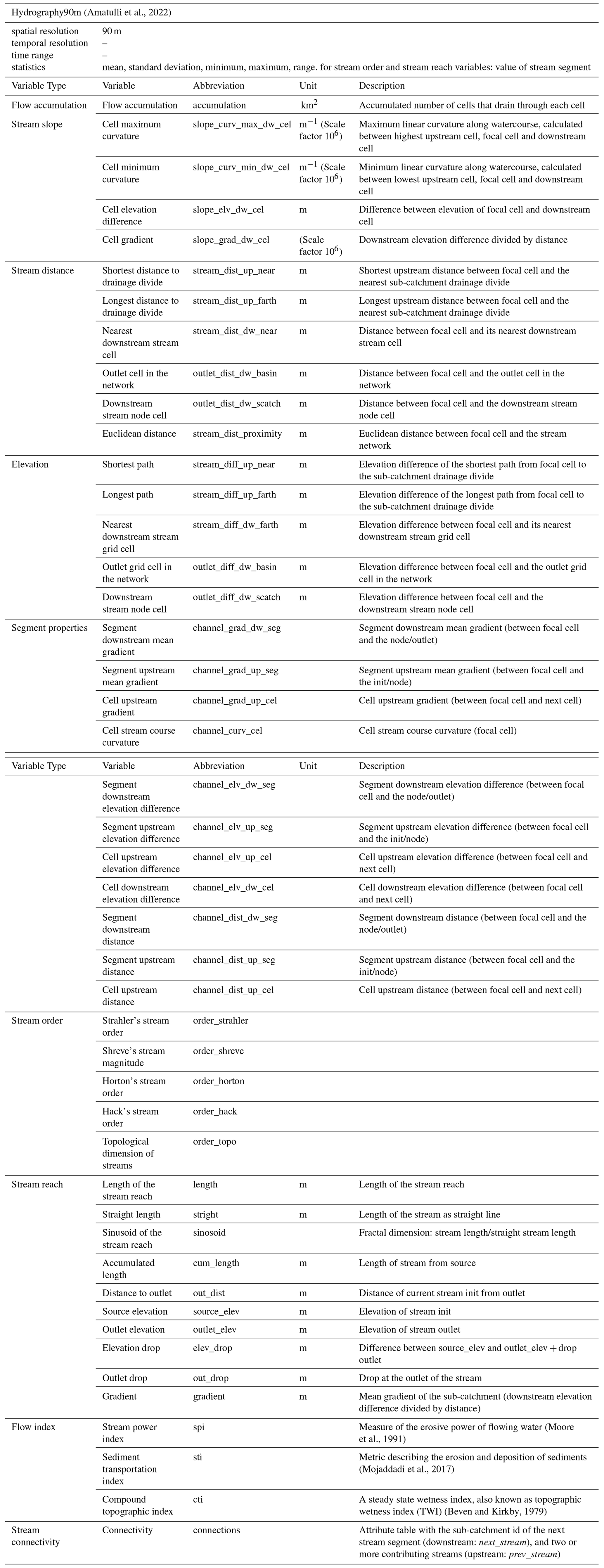
The Hydrography90m is a high-resolution (∼ 90 m) dataset delineating a global stream channel network (Amatulli et al., 2022) and serves as the basis of Environment90m. The calculation of Hydrography90m used the MERIT Hydro Digital Elevation Model at 3 arcsec (∼ 90 m at the Equator) (Yamazaki et al., 2017). The main feature of Hydrography90m is the delineation of small headwater streams. In addition, this dataset includes a number of stream topographic and topological properties (see Table 1), which have already been used for freshwater habitat analyses (e.g., Schürz et al., 2025).

(Amatulli et al., 2022)Moore et al., 1991Mojaddadi et al., 2017Beven and Kirkby, 1979

Table 1 List of variables derived from the Hydrography90m dataset. The original values of each variable are assigned on a 90m raster cell basis. A focal cell refers to the target cell or pixel where the calculation of the variables is being done. The term init refers to the initial node of a stream segment, i.e., the most upstream cell. The scale factor attached to the units column should be applied to calculate the real values.

2.2.2 Climate

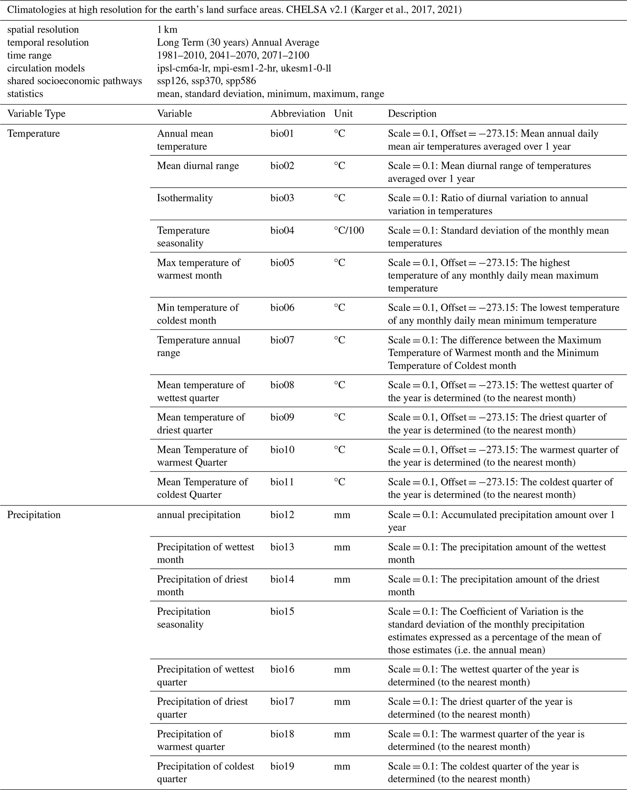
We derived high-resolution climate variables from the CHELSA v2.1 dataset available at “https://chelsa-climate.org/ (last access: 4 February 2026)” (Karger et al., 2017, 2021). We used 19 bioclimatic variables (bio 1 to 19) at 30 arcsec (ca. 1 km) resolution (Table 2). We aggregated the reference period available as a long-term annual average (1981–2010). Data for future climate projections (i.e., periods 2041–2070 and 2071-2100) were aggregated by selecting individual pairings of three global circulation models (GCMs, i.e., mpi-esm1-2-hr, ukesm1-0-ll, ipsl-cm6a-lr) and three Shared Socioeconomic Pathways (SSPs, i.e., SSP1-RCP2.6 [Sustainability – lowest emission scenario], SSP3-RCP7 [Regional Rivalry – middle emission scenario], and SSP5-RCP8.5 [Fossil Fuel Development – highest emission scenario]; Ebi et al., 2014; O’Neill et al., 2017). With this selection we cover short and long term future projections, and a wide spectrum of potential future trajectories given social, technological, economical and environmental changes. This diversity of options should facilitate the evaluation of uncertainties in climate projection exercises. Since its publication, the CHELSA v2.1 dataset has been used in studies on the suitability of Natura 2000 freshwater habitats for threatened species (e.g., Basen et al., 2022). It has also been used to track the niche and distribution dynamics of invasive freshwater fauna (e.g., Guareschi et al., 2024).

(Karger et al., 2017, 2021)

Table 2 List of variables derived from the CHELSA dataset. The scale and offset values provided in the description of some variables are factors used to convert the raw values to meaningful values, for example from raw data to Celcius degree for the temperature related variables. The equation to apply the factors is Corrected Value $=(\text{Raw Value}\times \text{Scale})+\text{Offset}$.

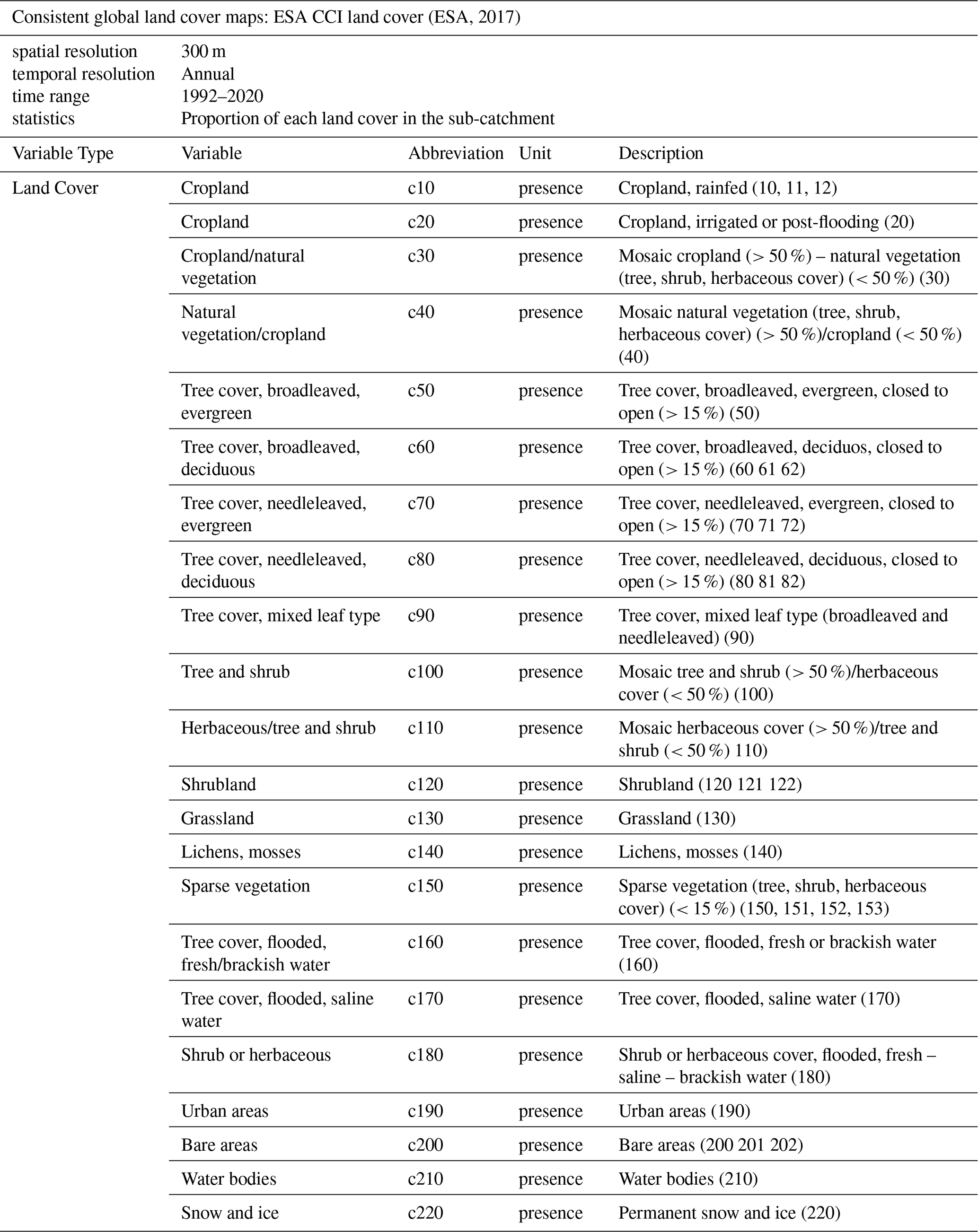
2.2.3 Land cover

For land cover data, we used the consistent global land cover maps of the Land Cover European Space Agency (ESA) Climate Change Initiative (CCI) project (ESA, 2017). We calculated the proportion of each land cover within the sub-catchments. We used level 1 land cover categories, which consists of 22 categories (Table 3) developed to describe land cover patterns globally. The 22 categories were selected based on their consistency in global coverage over the entire time period outlined in the Land Cover CCI product user guide (ESA, 2017). The annual data are available for the years 1992 to 2020. The ESA CCI land cover data have been useful in research that aims to identify patterns and hotspots of global land cover transitions (Liu et al., 2018). Other researchers have used the dataset to e.g. enhance water balance analyses in tropical regions (Tan et al., 2021).

(ESA, 2017)

Table 3 List of variables (i.e., land cover categories) derived from the ESA land cover maps. The numbers within parentheses in the description make reference to the coding of the land cover categories at level 2.

2.2.4 Soil

The soil variables were sourced from the global gridded soil information dataset, SoilGrids250 v2.0 (Hengl et al., 2017). This dataset represents global chemical and physical soil properties (Table 4). Each of the variables was originally provided at six standard depths (with the exception of depth to bedrock and soil organic carbon content) and at a spatial resolution of 250 m. To integrate all available soil depths (up to 200 cm), we calculated the weighted average for each soil property originally measured at different depths, following the GlobalSoilMap specifications described in Arrouays et al. (2014).

(Hengl et al., 2017)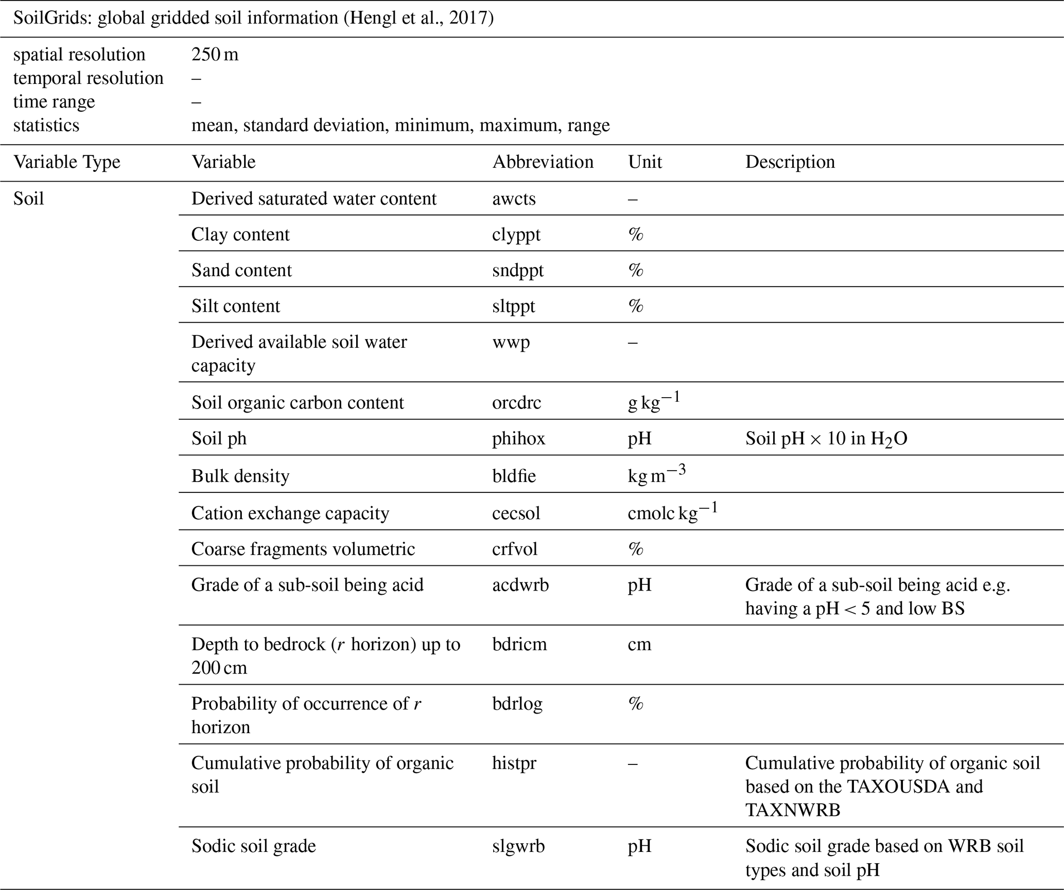

Table 4 List of variables derived from the SOILGRID database.

2.2.5 Elevation

To represent elevation we used the 90 m resolution Multi-Error-Removed Improved-Terrain Digital Elevation Model (MERIT DEM) (Yamazaki et al., 2017) (Table 5). The error removal procedures applied to this dataset have improved its vertical accuracy. This dataset was also used as the basis for the creation of the Hydrography90m dataset (Amatulli et al., 2022). Other research has made use of the MERIT DEM to enable machine learning-based estimations of dynamic water depth and volume of global lakes (Lv et al., 2025), or to conduct and subsequently evaluate continental-scale river hydrodynamic modelling (Modi et al., 2022).

(Yamazaki et al., 2017)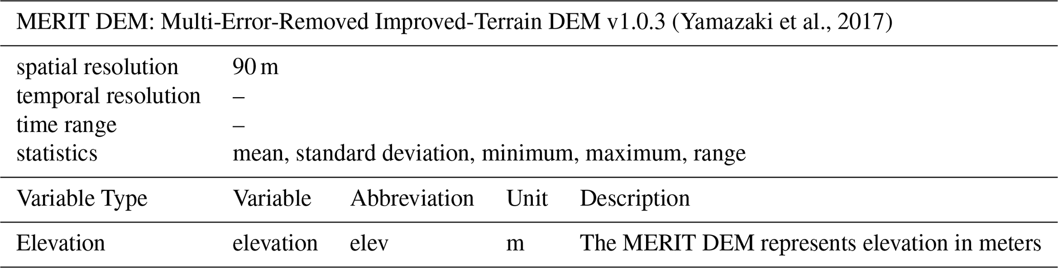

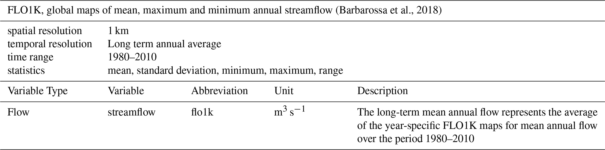
Table 5 List of variables derived from the MERID DEM.

2.2.6 Stream flow

For stream (water) flow we used the FLO1K dataset which comprises the modelled mean, maximum and minimum annual flow for each year in the period 1960–2015, provided as spatially continuous gridded layers at 30 arcsec (ca. 1 km) (Barbarossa et al., 2018) (Table 6). For Environment90m, we only used the data from 1980–2010 and averaged the data across this time frame, to match the CHELSA observed climate dataset (Sect. 2.2.2).

(Barbarossa et al., 2018)

Table 6 List of variables derived from the FLO1K streamflow dataset.

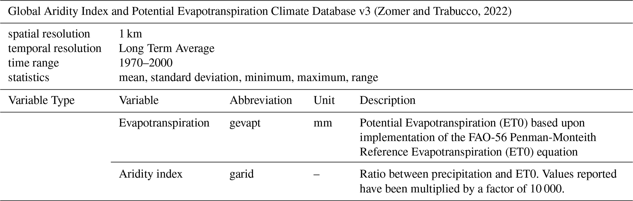
2.2.7 Global Aridity Index and Potential Evapotranspiration

This dataset provides high-resolution (30 arcsec, ca. 1 km) global raster data on evapotranspiration patterns and rainfall deficit for potential vegetation growth. Global Aridity and Potential Evapotranspiration are both modeled using data available from WorldClim Global Climate Data. The data is available for the 1970–2000 period (Zomer and Trabucco, 2022) (Table 7). Since its publication, the Global Aridity and Potential Evapotranspiration dataset has been used e.g. in data-driven modelling of freshwater ecosystems in Europe (Almeida and Cabral, 2023), as well as for the development of a global data set on drainage systems (He et al., 2024).

(Zomer and Trabucco, 2022)

Table 7 List of variables derived from the Global Aridity and Evapotranspiration dataset.

2.3 Accessing the Environment90m dataset

The initial set of tables contained the environmental information for all sub-catchments within each RU (see Sect. 2.1). These tables have been integrated into a PostgreSQL database as a backbone for the GeoFRESH online platform (available at https://www.geofresh.org, last access: 4 February 2026, Domisch et al., 2024) (Fig. 1), where users can interactively retrieve the data for any location of interest. The graphical user interface allows to upload point coordinates to the portal, move (or “snap”) the coordinates to the Hydrography90m stream network, and annotate the coordinates with Environment90m variables (Domisch et al., 2024).

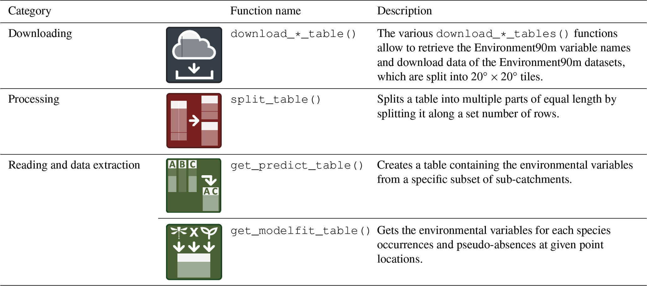
In addition, all tables were converted to follow the same tiling scheme as in the Hydrography90m dataset, such that the Environment90m and Hydrograhy90m datasets are compatible regarding the downloading and processing functionalities of the hydrographr R-package (Schürz et al., 2023). A number of new functions have been added to the hydrographr R-package specifically created to download and extract information from the original tables to specific subsets of target sub-catchments (Table 8). Although processing data frames in R is usually easy, the added value of the new functions is to overcome with challenges related to the size of the tables, especially at large geographical extents, and to process and e.g. subset the large tables efficiently using R-commands. The main feature of the hydrographr R-package is that it uses open-source third-party command-line tools without actually reading the data into R, such that large data files can be efficiently processed using R (Schürz et al., 2023). The next section presents a workflow to illustrate the use of the new available functions. Similarly, the tables in the tiling system can be manually and directly downloaded from the https://hydrography.org/environment90m (last access: 4 February 2026) website, by a point-and-click selection of the variables and tiles of interest.

Table 8 New functions added to the hydrographr R-package to download, process and extract information from the Environment90m dataset.

3 Case study: fish habitat suitability in the Danube River Basin

The Environment90m database is especially suited for freshwater biogeographic analyses, including predictive modelling of freshwater species distributions. This task usually requires range-wide spatial and environmental data, which can become massive when working at high resolution and large spatial extents. To facilitate the acquisition and processing of the large tables of Environment90m, and to enable a seamless integration with the Hydrography90m network, we have developed additional functions in the hydrographr R-package (Schürz et al., 2023) (see also Sect. 2.3). The following case study illustrates an example workflow to create a habitat suitability map of the Danube streber Zingel streber, a freshwater ray-finned fish in the family Percidae (Fig. 3). We provide the workflow at Case study – Danube (Environment90m) (https://glowabio.github.io/hydrographr/articles/case_study_Danube.html, last access: 4 February 2026). The main objective of the workflow is to showcase the computational efficiency of the hydrographr R-package in processing the large environmental tables for a simplified predictive modelling example.

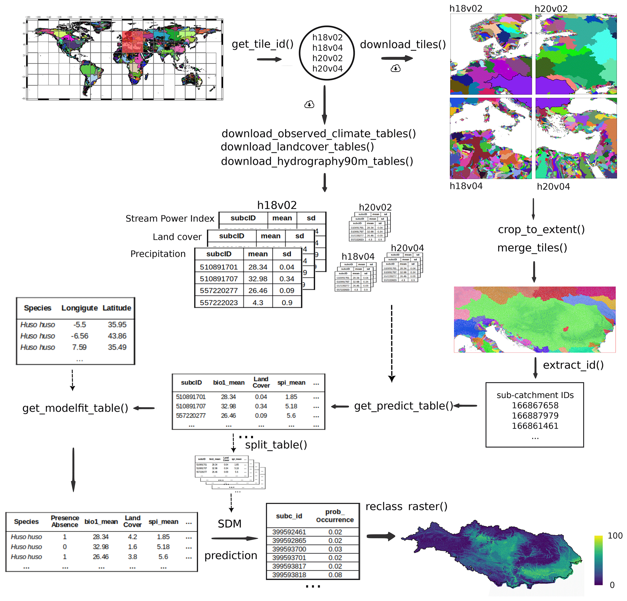
Figure 3 Workflow illustration for the case study of calculating the habitat suitability of a freshwater fish species, the Danube streber (Zingel streber), in the Danube River Basin. The diagram shows the new functions available in the hydrographr R-package to download the tables with the variables available in the Environment90m dataset, merge them for the area of interest and join the tables with species occurrence data as inputs to species distribution models (SDMs).

The first step is to identify the 20° × 20° tiles that overlap with a bounding box polygon of the Danube River Basin by applying the function get_tile_id(). Since the units of analysis to model the distribution of the species are the sub-catchments, we need to download the raster files of sub-catchments for each of the tiles using the download_tiles() function, crop each tile to the extension of interest with the function crop_to_extent() and merge the pieces of each tile with the function merge_tiles() to obtain a final raster file of sub-catchments for the bounding box of the Danube basin.

A parallel task is to download the corresponding Environment90m tables for each tile of the selected environmental variables. There are a number of functions dedicated to download each of the available datasets (e.g. download_landcover_tables()). The tables will be downloaded to disk and from here, they can be subset and merged, for example to process only those sub-catchment IDs that are present in the area of interest, in our case the Danube River Basin. This processing is done with the new function get_predict_table() which uses as arguments (i) the path on disk where the downloaded tables are located, and (ii) the list of sub-catchment IDs which have been previously identified, using the function extract_ids() on the sub-catchment raster file of the area of interest. Here, either all or only a subset of the aggregation statistics (e.g., mean, range) can be selected.

The output is a large table (i.e., the so-called range-wide “prediction table”) with all the sub-catchments of the area of interest and the values of the selected environmental variables. This table is still on disk, and for initial screening, a subset of it can be loaded into R to run exploratory or correlation analyses to make a selection of uncorrelated variables if the purpose is to e.g. quantify species ecological niches.

The species distribution modelling requires as input a table relating the species occurrence locations with the environmental data at those locations (i.e., the so-called “model-fit table”). The function get_modelfit_table() creates this table by combining (i) a table of species geographic locations (i.e., coordinates), (ii) the previously created range-wide prediction table, and (iii) the raster of sub-catchments generated during the first steps of the workflow. The model-fit table should contain the species occurrences and absences (or pseudo-absences) and their associated environmental values. The user can provide the occurrences and absences together. Alternatively, the function offers the possibility to create a user defined number of random pseudo-absences.

The model-fit table can be imported into R, where any modelling technique (e.g., Random Forest) can be applied to estimate the ecological niche of the species and predict the probability of habitat suitability of the species in the area of interest. The prediction itself is done by calling the model that has been previously fit and the “prediction table” we created before. Depending on the extent of the area of interest, the prediction table could be very large and reading the table into any statistical software or even running the prediction itself could be computationally unfeasible. To make the prediction calculations feasible, the large prediction table could then be split into several sections (using the split_table() function) and the prediction could be applied to each part in turn. The single output tables can be merged later. The final prediction table consists of each sub-catchment ID and its corresponding probability of occurrence value. This table can then be used with the reclass_raster() function to reclassify the original sub-catchment raster file to create a new raster file that shows the probability of habitat suitability of the species.

4 Case study: environmental characterization of lakes' upstream basins

We acknowledge that Environment90m focuses mainly on lotic habitats. To extend the data usage also to lentic habitats, we offer the possibility to extract Environment90m data not only for rivers but also across lakes and their contributing catchments. We provide an example code in a vignette, available at https://glowabio.github.io/hydrographr/articles/case_study_lakes.html (last access: 4 February 2026).

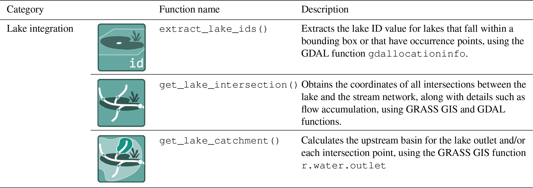
We have created three new functions, extract_lake_ids(), get_lake_intersection() and get_lake_catchment() (Table 9) that are available in the hydrographr R-package. Specifically, they allow (i) to identify the location of a lake within the Hydrography90m stream network, (ii) to obtain the intersection points between lakes and the stream network and (iii) to delineate for each intersection point the upstream lake catchment area (Fig. 4). All functions are built on each other. For instance, the extract_lake_ids() function enables to retrieve lake IDs either within a specified area through a bounding box or at given point locations. The lake IDs can then be used in the get_lake_intersection() function specifying the lakes of interest to identify the stream cells that intersect the lakes outline and the stream network. Additionally, the resulting intersection table, containing all intersection points of the lake and stream network, includes information on flow accumulation (mean and maximum values), its coordinates and the unique stream segment ID of the Hydrography90m stream network. From this we can delineate the upstream catchment area with the get_lake_catchment() function for any intersection point. The intersection point with the highest flow accumulation value represents the lake outlet covering the entire upstream lake catchment area. These functions then allow to extract the environmental variables across the upstream catchment area for any lake connected to the network. For instance, by using the land cover data time series in Environment90m, it is possible to quantify the annual land cover changes in the catchment area. The vignette uses the HydroLAKES dataset (Messager et al., 2016), though the functionality is generic for any lake vector dataset. In the GeoFRESH platform, currently only HydroLAKES are available (Domisch et al., 2024).

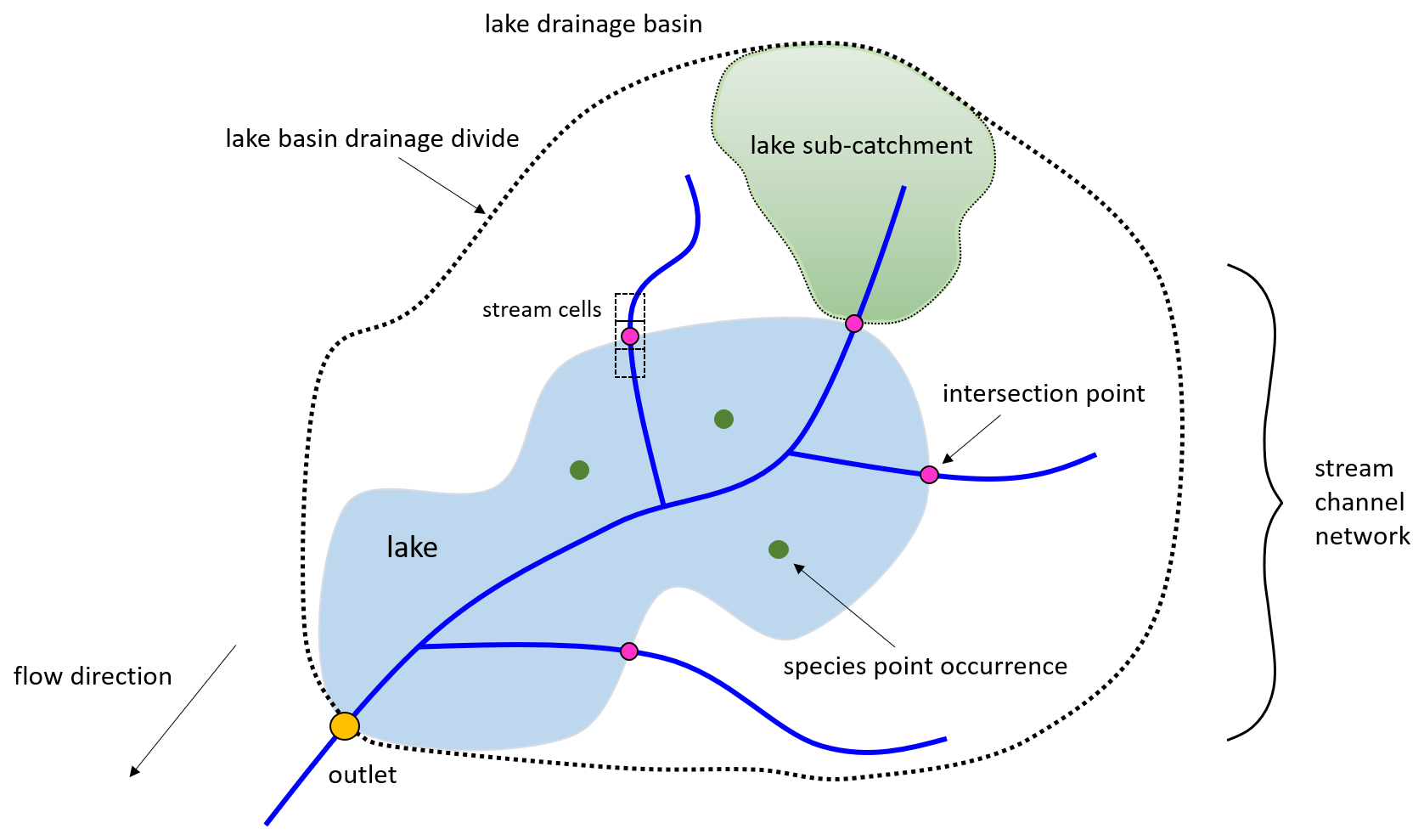
Figure 4 Schematic overview of the lake integration into the Hydrography90m stream network; accessible through the new hydrographr lake functions. See the main text for a detailed description.

Table 9 New functions added to the hydrographr R-package to integrate lakes with stream network and summarize information from the Environment90m dataset to lake upstream catchments.

5 Applications

The availability of globally standardized environmental data that address the structure of the hydrographic network enables comparative studies between regions. It facilitates large-scale biogeographic analyses in the freshwater realm and makes Environment90m particularly valuable for global-scale freshwater biodiversity research. For instance, a recent study focusing on the Guineo-Congolian region, a biodiversity hotspot in the Afrotropics, integrated stream network attributes derived from Environment90m with macroinvertebrate occurrence records spanning 2890 sub-catchments and stream orders 1–12, enabling biogeographic analyses in a previously understudied region. Another application of Environment90m in large-scale biodiversity assessments is demonstrated by (Haase et al., 2023), who used the dataset to analyse temporal freshwater invertebrate diversity trends across Europe. To identify environmental predictors that might drive these trends, the study used topographic, climatic and land-use variables aggregated at the sub-catchment level.

In addition, Environment90m is the backbone of a recent global study on ecological niche breadths of aquatic insect genera worldwide, where a suite of environmental predictors, such as mean stream slope gradient, stream length, bioclimatic variables and soil characteristics, was extracted per sub-catchment. These variables formed the basis for characterizing genus-level niches using the Climate-niche factor analysis (CNFA) and assessing patterns of aquatic insect niche breadth across freshwater insect assemblages (Grigoropoulou, 2024, in review). Moreover, a study from the University of California focusing on how the extent of permafrost sets the drainage density in the Arctic (Vecchio et al., 2024) also used stream network variables, derived from Environment90m, to calculate the drainage density in arctic watersheds between 23.5 and 90° N latitude.

Although not using Environment90m directly, other authors have credited Hydrography90m as a source to derive and map headwaters and analyze streamflow dynamics, after using the dataset in their study on advancing science for global water protection (Golden et al., 2025). Such applications demonstrate the value of the Environment90m dataset for freshwater biodiversity research worldwide, where globally standardized data accounting for the network structure are needed.

6 Data availability

The metadata of the Environment90m dataset is stored at https://doi.org/10.18728/igb-fred-995.0 (García Márquez et al., 2025a).

The Environment90m data can be obtained from the following sources:

• The primary Environment90m data is available as zipped .csv-tables. The data comes in 20° × 20° tiles, covering the same geographic extent and structure as the Hydrography90m dataset. These tiles can be interactively downloaded from https://hydrography.org/environment90m (last access: 4 February 2026).

• We recommend downloading and attaching the tables to the Hydrography90m stream network using the hydrographr R-package (Schürz et al., 2023). We provide example code at https://glowabio.github.io/hydrographr/articles/case_study_Danube.html (last access: 4 February 2026).

• For single point occurrences (i.e. coordinates), we offer the possibility to upload these to the GeoFRESH online platform (Domisch et al., 2024), available at https://geofresh.org/ (last access: 4 February 2026), and extract and download the Environment90m data either for the focal sub-catchment, or the aggregated data for the upstream contributing area.

7 Code availability

We provide all code for creating the Environment90m dataset at https://doi.org/10.5281/zenodo.18483574 (García Márquez et al., 2025b).

8 Discussion

The Hydrography90m dataset provides globally standardized environmental information of seven different environmental datasets for a total of 104 single variables within each of the 726 million sub-catchments of the Hydrography90m dataset. The Environment90m dataset is available in different formats (see Sect. 2.3) and can be seamlessly integrated with different tools (e.g., hydrographr R-package, The GeoFRESH platform) and integrated into workflows to create and advance novel freshwater-specific studies (see vignette examples).

The use of the sub-catchment as the spatial unit of analysis to summarize the environmental information has numerous advantages for freshwater ecosystem and biodiversity analysis, in contrast to the use of e.g. raster cells, as commonly done in terrestrial biogeographic analyses. Habitats and organisms are strongly defined by the topographical and topological influences of their surrounding environment and sub-catchments encompass these fluxes. Moreover, aggregating upstream sub-catchments can provide a more comprehensive understanding of the influences that fluxes and nature-state characteristics of upstream areas have on downstream habitats. In general, the information on the connection between sub-catchments opens the door to new type of analyses where network routing, river connectivity and fragmentation processes can be considered.

We also see the calculation of summary statistics for each sub-catchment as an advantage given the increase in the variety of explanatory variables that are important for understanding the distributions of freshwater habitats and biodiversity. Instead of characterizing a single sub-catchment only by the mean of a variable, e.g., elevation, the inclusion of standard deviation, or the minimum and maximum values can provide a measure of the variability of elevation in the sub-catchment. For instance, high standard deviation would represent a sub-catchment in a steep terrain, which cannot be represented only by the mean.

Although we incorporate variables that are commonly used in freshwater biogeographic analyses, there are more variables available globally that could be incorporated to the Environment90m dataset. In the near future we will add the remaining future climate projections, i.e., GCMs and time period (2011–2040). We did not include point-based data (such as nutrient or water quality measurements), and likewise focused on high-resolution environmental data. Thus, we recognize that other important variables for freshwater ecosystems may be missing in Environment90m. The challenge is, however, that coarse and gridded data, such as the global nitrogen fertilizer application map (Nishina et al., 2017) at approx. 50 km spatial resolution, can not be easily attributed to single stream segments or sub-catchments. For more regional or local studies, these type of layers would not be compatible with the Environment90m datasets. We plan to include further variables, such as the annual stream flow estimates of the FLO1K dataset (Barbarossa et al., 2018).

Taken together, we expect that Environment90m offers a unique possibility in analysing the environmental contingencies of freshwater habitats at high spatial resolution. Moreover, the dataset supports biogeographic analyses of freshwater habitats and biodiversity, and contributes towards the recent freshwater biodiversity conservation targets by providing a solid and globally standardized baseline of high-resolution environmental information.