1 km annual forest cover and plant functional type dataset for China from 1981 to 2023

High-spatial-resolution and long-term data on forest cover and plant functional types (PFTs) are crucial for elucidating the effects of forest cover change on the national terrestrial carbon balance. Since the 1980s, China has experienced a substantial expansion in its forested area, primarily driven by large-scale national afforestation programs. However, existing land cover products often fail to capture this long-term increasing trend, leading to an underestimation of forest cover change–related ecological processes. Here, we developed a high-resolution (1 km), annual forest cover dataset for China for 1981–2023. This dataset integrates spatial constraints from multisource remote sensing data with provincial-level statistics from China's national forest inventories (NFIs), providing a consistent and spatially explicit record of forest dynamics over four decades. Building on this primary dataset, we further produced an annual PFT dataset that disaggregates total forest cover into nine distinct plant functional types suitable for use in dynamic global vegetation models (DGVMs). Validation against independent data indicates that our reconstructed dataset achieves an overall accuracy (OA) of 84.86 % ± 1.18 % for five aggregated forest types (evergreen needleleaf forests, evergreen broadleaf forests, deciduous needleleaf forests, deciduous broadleaf forests, and mixed leaf forests), and it reproduces NFI-consistent forest dynamics (R²≈1). To evaluate its applicability, we implemented the dataset in the Lund–Potsdam–Jena General Ecosystem Simulator (LPJ–GUESS). Compared with the widely used PFT dataset from the European Space Agency's Land Cover Climate Change Initiative (ESA CCI) and the MODIS land cover type product (MCD12Q1), our product yields a markedly improved simulation of key biophysical and biogeochemical processes in China. Specifically, it reduced errors relative to over extensive regions, outperforming these baselines across 77.7 % and 85.2 % of the terrestrial area for gross primary productivity (GPP), 63.1 % and 69.7 % for net ecosystem exchange (NEE), 66.9 % and 77.3 % for the leaf area index (LAI), and 78.7 % and 85.3 % for actual evapotranspiration (ET). With its high spatial resolution, long-term temporal coverage, and detailed forest type classification, our dataset offers a robust foundation for assessing the ecological impacts of forest restoration and for constraining estimates of China's forest carbon sink since 1981. The dataset is freely available at https://doi.org/10.5281/zenodo.18448036 (Liu et al., 2026).

1 Introduction

Large-scale afforestation programs have been implemented in China during the past four decades (Tong et al., 2018; Chen et al., 2019). As a result, compared with that in the early 1980s, the forestland area in China increased to approximately 230 million  ha, a rise of 100 % (IDS, 2018). Recent satellite observations revealed widespread “vegetation greening patterns” in China because of several large-scale conservation programs (Piao et al., 2020). These changes have had significant implications for carbon dynamics and ecosystem services. Specifically, they have increased carbon sequestration, reduced soil erosion and acidification in northern China, and altered regional climate patterns through changes in surface albedo, evapotranspiration, and aerodynamic roughness (Liu et al., 2017; Hong et al., 2020). These findings underscore the critical role of afforestation in mitigating climate change and improving ecosystem stability at regional and global scales (Alkama and Cescatti, 2016; Yang et al., 2024).

Despite these positive developments, precisely quantifying the contributions of these land cover changes to the global carbon balance remains a significant challenge (Li et al., 2025; Yu et al., 2024). During the period from 2014–2023, the net carbon emissions from the global land use, land use change, and forestry (LULUCF) sector were estimated at 4.1 ± 2.6 Gt CO₂ yr⁻¹, accounting for 10 % of total anthropogenic CO₂ emissions (Friedlingstein et al., 2025). The uncertainty of this estimate exceeds 50 % of the mean flux, making LULUCF the most uncertain component in the global carbon budget (Friedlingstein et al., 2025; O'Sullivan et al., 2022). These uncertainties primarily arise from disparities in model process representation, inconsistencies in flux definitions, variability in management practices, and spatiotemporal estimation differences in forest cover and its rate of change (Ruehr et al., 2023; Hartung et al., 2021; Yu et al., 2022).

Although remote sensing has greatly improved the availability of land use and land cover (LULC) data, discrepancies among different datasets regarding the estimation of China's forestland area have led to large uncertainties in modelling (Tu et al., 2024; Zhu et al., 2025); for instance, three- to fivefold differences in estimates of China's terrestrial carbon storage have been reported from similar bookkeeping models (e.g., 17–33 Pg C vs. 6.18 Pg C from 1700 to 2000) (Houghton and Hackler, 2003; Ge et al., 2008). Cross-dataset comparisons highlight the scale of this issue: estimates of China's forestland area for the year 2010 from five different forest datasets ranged from 1.74 to 2.27 million  km², a relative difference of 29 % (Qin et al., 2015). Peng et al. (2024b) compared eight LULC datasets for the year 2020 and reported a maximum discrepancy of 0.34 million  km², an amount equivalent to 15 % of the area reported by the national forest inventory (NFI). This interproduct inconsistency is notable, as it appears to be inconsistent with the widely reported trend of forest expansion in China. According to NFI data, the nation's forestland area more than doubled from 1.15 million  km² in 1981 to 2.31 million  km² by 2021 (IDS, 2018). This trend is consistent with broader assessments by the Food and Agriculture Organization (FAO) of the United Nations, which attributed the shift in Asia's forest balance from a net loss in 1990–2000 to a marked net gain in 2000–2010 primarily to China's sustained afforestation efforts (FAO, 2016). However, long-term satellite-based LULC products often fail to capture this marked increase (Yang and Huang, 2021a). For example, the GlobeLand30 product shows a relatively small expansion of 5700 km² between 2000 and 2020 (Chen et al., 2015), while the national land cover database of China (NLCD–China) indicates a net loss of 14 000 km² from 2001 to 2015 (Wei et al., 2024). Consequently, owing to these differences among datasets, the contribution of the LULUCF sector to China's regional carbon budget is subject to uncertainty (Xia et al., 2023; Yu et al., 2022).

The NFI is considered the foundational national dataset for quantifying forest cover and biomass stocks (Zeng et al., 2015; Xia et al., 2023). Since the implementation of the second NFI from 1977–1981, a standardised sampling and survey methodology has been applied nationwide. Eight further NFI campaigns were subsequently conducted on a continuous 5 year cycle (IDS, 2018). Owing to its extensive sample size covering the entire country, the forest area statistics provided by the NFI are widely regarded as a reference dataset. This large-scale inventory provides unique bottom-up information that complements top-down data from satellite remote sensing products, ensuring that the spatiotemporal dynamics of land use activities are accurately captured. Previous studies have utilised the NFI dataset to estimate the national forest carbon budget (Fang et al., 2001; Piao et al., 2009). However, a key limitation of the NFI is that it only publicly provides forest area statistics at the coarse provincial level. This spatial aggregation constrains its direct application for simulating carbon dynamics in spatially explicit earth system models (Zhu et al., 2025).

At both global and national scales, dynamic global vegetation models (DGVMs) typically represent key vegetation processes – such as photosynthesis and evapotranspiration – using a simplified classification of globally representative plant functional types (PFTs) that exhibit similar ecological and physiological traits (Gregor et al., 2024; Bergkvist et al., 2025); they are typically defined by traits such as photosynthetic pathway (${\mathrm{C}}_{\mathrm{3}}/{\mathrm{C}}_{\mathrm{4}}$), leaf morphology (needleleaf/broadleaf), and phenology (evergreen/deciduous) (Islam et al., 2024). Research has shown that explicitly incorporating forest restoration processes into DGVMs is critical not only for quantifying their feedback on the carbon cycle, surface energy balance, and climate system but also for providing a science-based foundation for policy assessment (Yue et al., 2024; Peng et al., 2024a). To accurately simulate carbon dynamics and vegetation succession, these models need to be driven by annually updated PFT distribution data (Pugh et al., 2024). However, a high-resolution, annual time series dataset that accurately reflects the PFT composition and spatial distribution during China's recent forest restoration is currently lacking (Yu et al., 2022; Xia et al., 2023). Most existing forest cover products provide either single-year classifications or PFT information at a coarse temporal resolution, failing to meet the annual input requirements of DGVMs (Ran et al., 2012). Furthermore, they often fail to capture the forest recovery trends documented by the NFI. While some recent studies have developed NFI-based reconstructed forest datasets, these products are typically either too coarse in spatial resolution, do not provide the distribution of individual PFTs, or are not temporally continuous, with maps produced only every few years (Yu et al., 2022; Xia et al., 2023). Therefore, there is an urgent need to generate NFI-consistent, high-resolution, and annually resolved long-term maps of both forest cover and the PFT distribution. Such a dataset is fundamental for robustly assessing China's forest carbon sink and its driving factors using ecosystem models.

In this study, we developed a novel method that combines temporal constraints from statistical inventories with spatial constraints from remote sensing data to identify the distribution of forest PFTs. We integrated provincial-level forest area statistics from the NFI for 1981–2023 with nearly all available LULC and auxiliary remote sensing products. This allowed us to first reconstruct annual changes in China's total forest cover at a 1 km spatial resolution from 1981 to 2023. Building on this foundation, we then derived the annual distribution of nine distinct PFTs for the period 1981–2023 through a series of systematic steps, including the classification of life forms and the derivation of phenological characteristics. The overall goal of this work is twofold: first, to provide a dataset that accurately captures the spatiotemporal distribution and trends of China's forests and PFTs since the onset of its national restoration programs in the 1980s, and second, to demonstrate the effectiveness of this new dataset in a DGVM. To achieve this goal, we applied our product in the Lund–Potsdam–Jena General Ecosystem Simulator (LPJ–GUESS) model (Lindeskog et al., 2021) and benchmarked its performance against that achieved with the global PFT dataset from the European Space Agency's Climate Change Initiative (ESA CCI) (Harper et al., 2023) and the MODIS land cover type product (MCD12Q1) (Sulla-Menashe et al., 2019) in simulating key land surface variables, namely gross primary production (GPP), net ecosystem exchange (NEE), the leaf area index (LAI), and actual evapotranspiration (ET). We present the following: (1) changes in China's forest cover and PFTs since the 1980s; (2) the historical dynamics of forest gain and loss, including the area, onset year, and duration; and (3) the performance of our reconstructed PFT distribution compared with those based on existing global datasets when used in a DGVM. Ultimately, our dataset is expected to provide critical data support for accurately simulating China's forest carbon sink and scientifically assessing the corresponding driving factors since the beginning of large-scale forest restoration at the national scale.

Table 1 Summary of the datasets used in this study.

2 Data

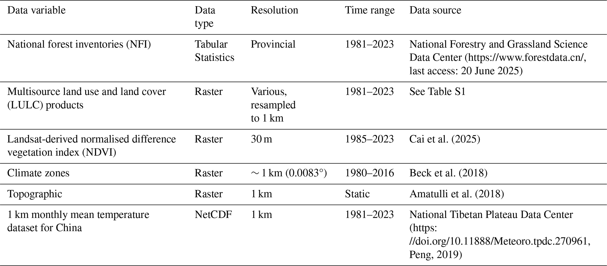
The forest cover and PFTs were derived from the integration of NFI data with multisource remote sensing LULC time series data (Table 1, Table S1 in the Supplement). The LULC data provides the spatial distribution of forest cover across different years. For specific years, land cover classification was used to define the extent of forest PFTs, based on distinctions in phenology and leaf morphology. The NFI data was used to constrain the forest area and structural composition; this ensured that the resulting dataset aligned with reported national trends in forest area dynamics.

Auxiliary data products, such as satellite-based normalised difference vegetation index (NDVI) data (see Sect. 2.3), were used to identify potential residual forestland pixels in cases of discrepancy between the LULC data and NFI data. For example, when the area of forestland cover extracted from the LULC data was less than the area specified by the NFI for a given region, the NDVI was used as a sensitive indicator of vegetation vigour. Pixels considered likely to represent forest cover were then selected to supplement the forest area and its spatial distribution.

2.1 National forest inventories

To assess the quantity, structure, function, and productivity of national forest resources, the National Forestry and Grassland Administration of China conducted ten national forest resource inventories between 1973 and 2023. The inventories took place during the periods 1973–1976, 1977–1981, 1984–1988, 1989–1993, 1994–1998, 1999–2003, 2004–2008, 2009–2013, 2014–2018, and 2019–2023. The data are available from the National Forestry and Grassland Science Data Center (NFGSDC) at https://www.forestdata.cn/ (last access: 20 June 2025). The surveys were performed at the provincial level, and a systematic sampling design with fixed plots located at the intersections of the national 1:50 000 or 1:100 000 topographic map grids were employed. For each plot, the recorded variables included forest cover, forest type area, and standing volume. Provincial-level area statistics from NFI report specifically, area data for wooded land, needleleaf and broadleaf forests from the second through eighth inventories; arbor forestland area from the ninth inventory; and total forestland area from the sixth through tenth inventories, were used in the analyses.

2.2 Land use and land cover datasets

In this study, twenty-two datasets covering the period 1981–2023 were utilised as the foundational inputs for forest cover reconstruction (Table S1). Forest cover information was extracted from these LULC products. Preprocessing of the data involved several steps: (i) reprojecting all the datasets to the WGS_1984_Albers spatial reference system; (ii) resampling to a 1 km resolution using the majority method; and (iii) aligning all the data to a common grid framework to ensure a consistent cell size and spatial extent for China.

2.3 Satellite-based vegetation index dataset

In this study, China's first seamless annual leaf-on (growing season) Landsat composite dataset (1985–2023) from Cai et al. (2025) was utilised. This dataset harmonises multisensor Landsat imagery through a comprehensive compositing method, addressing critical issues such as cloud/shadow contamination, reflectance consistency, and data gaps, thereby providing a single annual growing-season composite image. The dataset is available on the Google Earth Engine (GEE) platform (https://ee-caiyt33-catcd.projects.earthengine.app/view/landsat-yearly-composite-viewer, last access: 20 October 2025).

From this dataset, we derived annual growing-season NDVI data using the near-infrared (NIR) and red bands, calculated as follows: $(\mathrm{NIR}-\mathrm{Red})/(\mathrm{NIR}+\mathrm{Red}$). These data were then resampled to a 1 km resolution using mean aggregation. In this study, the growing-season NDVI served as the primary indicator for classifying “potential forestland pixels” as forestland (see Sect. 3.3). Owing to the scarcity of Landsat imagery in the early 1980s (Yang and Huang, 2021a) and to ensure temporal consistency across the extended 1981–2023 analysis period, records for 1981–1984 were gap-filled using data from 1985. To validate this substitution, we performed a pixel wise correlation analysis between the 1985 growing season NDVI and three independent, coarser resolution products covering 1981–1985 (Jeong et al., 2024; Li et al., 2023; Li et al., 2024), with all datasets processed as growing season (June–October) median composites and the 1985 baseline resampled to match the respective coarse resolutions. The results indicate that the 1985 dataset maintained high spatial consistency with the validation products (R² > 0.8). Furthermore, the correlation metrics exhibited exceptional temporal stability (ΔR² < 0.04; Fig. S1 in the Supplement).

Figure 1 Flowchart for generating annual forest cover and plant functional type (PFT) maps.

2.4 Zonation products

To assign phenological types to the small number of remaining unclassified forestland pixels (see Sect. 3.4.2), two supplementary regional partitioning products were utilised. The first was the Köppen–Geiger climate classification from Beck et al. (2018), which classifies Earth's land surface into 30 distinct climate zones at a 0.0083° resolution (approx. 1 km) on the basis of temperature and precipitation records from 1980–2016. The data are publicly available from Figshare at https://figshare.com/articles/dataset/Present_and_future_K_ppen-Geiger_climate_classification_maps_at_1-km_resolution/6396959/2 (last access: 26 May 2025). The second product was a global topographic dataset from Amatulli et al. (2018), derived from the 250 m GMTED2010 and 90 m SRTM4.1dev digital elevation models. In this dataset, the global land surface is classified into ten topographic categories: flat, peak, ridge, shoulder, spur, slope, hollow, footslope, valley, and pit. The data are publicly available from Earthenv at https://www.earthenv.org/topography (last access: 25 May 2025). In general, needleleaf forests are predominantly evergreen, with the notable exception of larch forests, which are deciduous and found mainly in boreal regions. In contrast, broadleaf forests are typically deciduous, although those in tropical regions are predominantly evergreen. To further classify evergreen and deciduous forest types as either boreal/temperate or tropical (see Sect. 3.4.3), the 1 km resolution monthly mean temperature dataset for China (1981–2023) from Peng et al. (2019a) was utilised. This dataset was generated by spatially downscaling the global 0.5° CRU climate dataset and the high-resolution WorldClim dataset using the delta spatial downscaling method. The data are publicly available from the National Tibetan Plateau Data Center (https://doi.org/10.11888/Meteoro.tpdc.270961, Peng, 2019).

3 Method

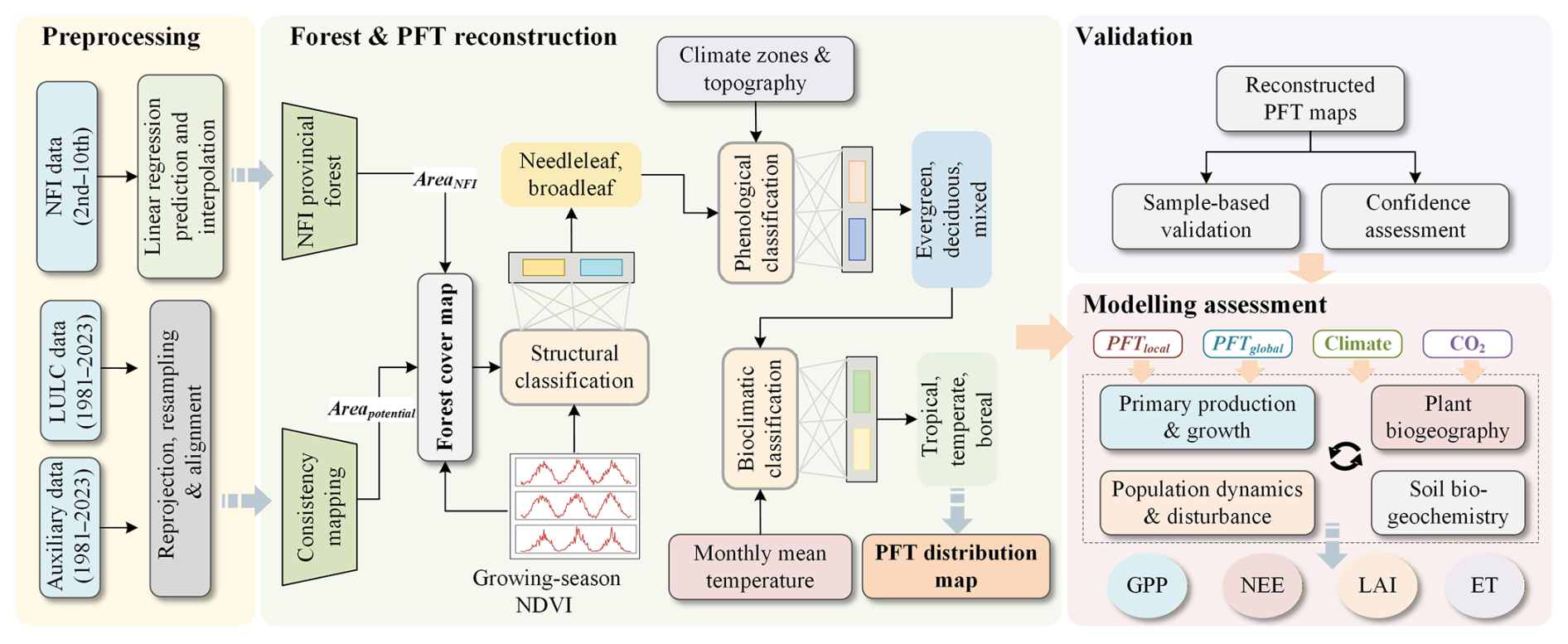
The framework for mapping forest cover and PFTs is shown on Fig. 1. It includes the interpolation of NFI statistical data, reconstruction of annual PFTs, validation, and modelling assessment. We constructed annual forest cover maps of China for the period 1981–2023 by integrating multiple data sources and derived PFTs through a sequential, multistep process. First, forest life forms were classified using a method analogous to that used in forest cover reconstruction; second, phenological characteristics were derived; and finally, these intermediate classifications were subdivided into the final PFTs on the basis of a set of climatic rules. Finally, the accuracy of the reconstructed dataset was assessed using validation samples from field surveys and independent reference data, and its consistency was analysed against existing LULC datasets. In particular, the reconstructed PFT dataset was used to drive a DGVM to evaluate the effectiveness of using the updated PFTs in simulating a series of surface fluxes by comparing the result with those obtained from simulation using the global PFT dataset from the ESA CCI (Harper et al., 2023) and the MCD12Q1 dataset (Sulla-Menashe et al., 2019).

Table 2 Classification and definitions of forest components.

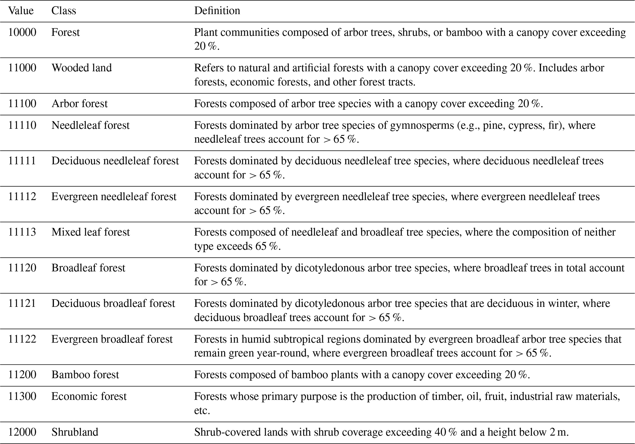
Note: Adapted from “Technical Regulations for Continuous Forest Inventory” (GB/T 38590-2020).

3.1 Definition of forest

A clear definition of forest composition is needed prior to reconstructing the PFT distribution. In accordance with China's “Technical Regulations for Continuous Forest Inventory” (GB/T 38590–2020), China's forests are divided into categories such as wooded land, arbor forestland, shrubland, bamboo forestland, and economic forestland, following a specific hierarchical classification system (Table 2). The area relationships among these components are defined as follows in Eqs. (1)–(3):

$$\begin{array}{}\text{(1)}& {\displaystyle }& {\displaystyle }{A}_{\text{Forest}}=A_{\text{Woodedland}}+A_{\text{Shrubland}}\text{(2)}& {\displaystyle }& {\displaystyle }{A}_{\text{Woodedland}}=A_{\text{Arbor}}+A_{\text{Bamboo}}+A_{\text{Econ}}\text{(3)}& {\displaystyle }& {\displaystyle }{A}_{\text{Arbor}}=A_{\text{Needleleaf}}+A_{\text{Broadleaf}}.\end{array}$$

Our reconstruction method adheres to two primary constraints: (1) Forest area constraint: To ensure consistency between statistics and remote sensing data, our “forest” class is constrained using the provincial-level area of wooded land. We explicitly exclude the shrubland category. This approach aligns our statistical constraint with the “forest” class (i.e., tree-covered areas) typically identified in LULC products, excluding the “shrub” category present in some LULC products. (2) PFT area constraint: The subclassification of PFTs is constrained using the provincial area of arbor forest, which comprises the needleleaf and broadleaf categories (Table 2). Notably, the NFI technical regulations specify that “mixed leaf forest” is included within the needleleaf forest area. This two-level constraint is used to determine the mapping approach used to identify potential forestland pixels by harmonising corresponding forestland classes from diverse LULC products, while ensuring that the reconstructed forestland area and the areas of our derived PFTs are strictly consistent with their corresponding NFI statistical areas.

3.2 Extrapolation and interpolation of NFI statistical data

To construct the continuous forest cover time series for 1981–2023, provincial forest areas from each NFI period were assigned to the final year of that period (e.g., data from the 1976–1981 survey were assigned to 1981) (Yue et al., 2024). However, owing to the latency in NFI data publication, the temporal coverage of statistical data varies by category. Notably, the statistics for wooded land, needleleaf forests, and broadleaf forests are available only up to the eighth inventory (2013); arbor forest statistics are available up to the ninth inventory (2018); and the total forest area is available up to the tenth inventory (2023). To address these data gaps, we extrapolated the missing values for the post-2013 period using linear regression models based on published data. This approach is supported by prior studies, which indicated that national afforestation targets exhibit a consistent linear trend over time, increasing by approximately 1.8 million  ha annually (He et al., 2024a; Xu et al., 2023).

Specifically, we first modelled the relationship between provincial total forest area and arbor forest area using available data from 2003–2018. We applied these models to extrapolate the arbor forest area for 2023, using the known 2023 total forest area as the predictor (Fig. S2; China R² = 0.97). Concurrently, using data from 2003–2013, we established linear regression models between total forestland area and wooded land area to preliminarily predict wooded land areas for 2018 and 2023. According to the definition in Sect. 3.1, the area of wooded land must be strictly equal to or exceed that of arbor forest. However, a comparison of our preliminary wooded land predictions from 2018 with the recorded arbor forest data from 2018 revealed logical inconsistencies in Tibet and Gansu Provinces, where the predicted wooded land area was smaller than the arbor forestland area. To rectify this difference, we adjusted the 2018 wooded land values for these two provinces to match their actual arbor forestland areas and reincorporated these corrected data into the model to predict the 2023 wooded land area. A final consistency check of the 2023 predictions revealed a similar discrepancy in Qinghai Province, which was adjusted accordingly to match the predicted arbor forest area (Fig. S3; China R² = 0.98).

Next, to estimate the needleleaf and broadleaf forestland areas for 2018 and 2023, we assumed that the growth trends observed from 2003–2013 persisted into the 2013–2023 period (Chini et al., 2021). Given that the arbor forestland area is the sum of the needleleaf and broadleaf forestland areas (see Sect. 3.1), we calculated the ratio of each forest type to the total arbor forestland area for 2003, 2008, and 2013. We then constructed linear regression models based on these historical ratios to project the corresponding proportions for 2018 and 2023. The final provincial areas for needleleaf and broadleaf forests were derived by multiplying these projected ratios by the (known or extrapolated) arbor forest areas for 2018 and 2023. Finally, once the areas for all benchmark years were established, we applied linear interpolation to fill the gaps in annual data between these benchmarks (Yu et al., 2022; Yue et al., 2024). All extrapolation and interpolation procedures were implemented independently for each province to account for regional heterogeneity in policies and environmental factors. Notably, arbor forest statistics are missing for Hong Kong, Macau, and post-2013 Taiwan. Given that China's major afforestation programs do not cover these regions, we did not reconstruct the arbor forest areas for Hong Kong, Macau, or post-2013 Taiwan (Zhang et al., 2025).

3.3 Forest cover reconstruction

In this study, a data-driven “forest consistency” method was developed to reconstruct historical forest cover (Fig. 1). The method involved overlaying all available LULC datasets for each year (Fig. S4). For any given pixel, “consistency” (CON) was defined as the number of datasets in which the pixel was classified as forestland (Fig. S5a). A pixel was subsequently identified as a “potential forest pixel” if it was classified as forest in at least one dataset (i.e., CON > 0). The consistency value was then used to establish priority, whereby a high CON value indicated a high likelihood of the pixel representing true forest cover (Xia et al., 2023; Fang et al., 2020).

To determine the consistency threshold for the final forest classification, all potential forestland pixels were ranked in descending order of their CON values. The NFI-derived area for a given province was used as the target value to establish this threshold. Specifically, two scenarios were considered. First, if the total area of all potential forestland pixels was less than the NFI-reported area, all potential pixels were classified as forestland, a scenario that could result in an underestimation for that province. Second, if the total area of potential pixels exceeded the NFI-reported area, a cumulative summation was performed. Pixels were incrementally summed, starting from the highest consistency value downwards, until the cumulative area bracketed the NFI target area (A_NFI). If the cumulative area of pixels with CON≥m was less than A_NFI but the cumulative area of pixels with $\mathrm{CON}\ge m-\mathrm{1}$ exceeded A_NFI, then m was defined as the consistency threshold. All pixels with a consistency value ≥m were subsequently classified as forestland. To precisely match the NFI target area, however, a portion of the remaining required area was filled by selecting pixels from the $\mathrm{CON}=m-\mathrm{1}$ level. On the basis of the assumption that, within a given consistency level, a high NDVI value indicates a high likelihood of forest cover existing, the growing-season NDVI was calculated for all pixels at the $\mathrm{CON}=m-\mathrm{1}$ level. These pixels were then ranked in descending order of their NDVI values. The top n pixels were subsequently selected as “residual forest pixels”, where n was determined on the basis of the remaining area required to precisely match the NFI target.

In summary, the final forest classification was performed to identify pixels that exhibited both high cross-dataset consistency and high growing-season NDVI values. The total area of this final classification was strictly constrained by provincial NFI statistics, thereby ensuring that the reconstructed maps aligned with the authoritative inventory data. While this method generally ensures a close correspondence to the NFI-reported area, minor systematic underestimation can occur. This is a consequence of pixel resolution limitations, particularly when the final area required to meet the NFI target is smaller than that of a single pixel.

3.4 PFT dataset development

3.4.1 Distinguishing between needleleaf and broadleaf forest types

Theoretically, the same reconstruction method used for total forest cover could be applied to directly classify five distinct PFTs: evergreen needleleaf, evergreen broadleaf, deciduous needleleaf, deciduous broadleaf, and mixed leaf forests. However, data availability constraints preclude the direct application of this method, since few LULC products offer this level of thematic detail, particularly for periods before 1990. For instance, for the year 1985, only a single available dataset differentiated between needleleaf and broadleaf forests, whereas for 1981, no dataset provided phenological classifications (i.e., evergreen vs. deciduous; Table S1). Consequently, a foundational assumption of this study is that the relative spatial distribution of these five PFTs remained static throughout the analysis period.

Extrapolation and interpolation of the NFI provide provincial-level forest area statistics for needleleaf and broadleaf forests for the period 1981–2023, but phenological classifications (i.e., evergreen vs. deciduous) remains limited. Therefore, the initial classification step in this study involved distinguishing between needleleaf and broadleaf forests within the previously reconstructed total forest extent.

To achieve this goal, nine LULC products containing forest type information were selected (Table S1). All available temporal layers from these nine products, amounting to 92 distinct data layers in total, were subsequently overlaid. Based on the previously stated assumption of a static PFT distribution, these 92 layers were used to generate two static consistency maps: one for needleleaf and one for broadleaf forests (Fig. S6). To ensure close spatial correspondence between this PFT classification and the main forest cover dataset, the static consistency maps were masked using the annual 1 km forest extent maps reconstructed in the previous step. This process generated annual consistency maps for each forest type, constrained within the total forest area for each respective year.

A critical preliminary step was required to adapt the main reconstruction method for distinguishing between needleleaf and broadleaf forests. The primary goal of this step was not to produce a final classification but to resolve conflicts among the source LULC datasets. This ensured that each pixel could be assigned a single, spatially exclusive “type-specific consistency” value, which is a prerequisite for the reconstruction logic that follows.

To achieve this, two consistency values were calculated for each pixel: needleleaf consistency (CON_need), representing the number of LULC datasets in which the pixel was classified as needleleaf forest; and broadleaf consistency (CON_broa), representing the number of datasets in which the pixel was classified as broadleaf forest. A rule-based approach was then applied to handle the three possible scenarios and assign a preliminary, exclusive status to each pixel:

1. Both consistency values are nonzero (CON_need>0 and CON_broa>0): The pixel's consistency type was determined by comparing the two values. If CON_need>CON_broa, the pixel was designated as a needleleaf consistency pixel. If CON_need<CON_broa, it was designated as a broadleaf consistency pixel. If CON_need=CON_broa, the pixel was flagged as “ambiguous”, and its classification was deferred to a later stage.

2. Only one consistency value is nonzero (e.g., CON_need>0 and CON_broa=0): The pixel was designated as a consistency pixel of the corresponding forest type for which the value existed.

3. Both consistency values are zero (CON_need=0 and CON_broa=0): The pixel was provisionally flagged as “unclassified forest type” in this step, with its final status to be determined later.

The second major step involved generating annual distribution masks for needleleaf and broadleaf forests for each province for the period 1981–2023. This was achieved by integrating provincial NFI area statistics with type-specific consistency information. In a process analogous to total forest cover reconstruction, the NFI area statistics for needleleaf and broadleaf forests were used as annual targets. The specific allocation logic, which uses NDVI data as a secondary criterion, depended on the relationship between the consistency-derived area and the NFI target area. This resulted in three distinct cases:

1. Both forest types have “valid” consistency data (i.e., the total potential area from the consistency map exceeds the NFI target area). In this scenario, the allocation method described previously was applied independently to each type. The consistency threshold (m) was determined, and the remaining area required to meet the NFI target was filled by selecting pixels from the CON = m−1 level, ranked in descending order of their growing-season NDVI value.

2. Only one forest type has “valid” consistency data. The “valid” type was processed first, following the same procedure as in Case 1. For the “invalid” type (where the potential area was less than the NFI target), a hierarchical sourcing strategy was used to reach its NFI area target. Pixels were drawn sequentially from the following pools, using the NDVI ranking method for selection at each stage:

   First, the pixels are drawn from the pool of those flagged as “ambiguous” (CON_need=CON_broa).

   Second, pixels are drawn from the pool of unallocated pixels of “valid” type. This involved using the “remainder” pixels from the “valid” type consistency map (i.e., those not selected to reach the corresponding NFI target) to mask the original consistency map of the “invalid” type. From this newly masked map, pixels were selected in descending order of their consistency value until the NFI area target for the “invalid” type was filled.

   Third, pixels are flagged as an “unclassified forest type”.

3. Neither forest type has “valid” consistency data. In this case, both NFI area targets were achieved by drawing pixels exclusively from the “ambiguous” and “unclassified forest type” pools. The allocation was prioritised for the provincially “dominant” type (i.e., the type with the larger NFI area). Once this target was met, the remaining pixels from these pools were allocated to the other forest type. An NDVI ranking method was used for all selections.

Finally, this process resulted in the output of annual needleleaf and broadleaf forest distribution masks for the specified period.

3.4.2 Distinguishing among evergreen, deciduous, and mixed-leaf forest types

In a process analogous to the classification of needleleaf and broadleaf types, further classification was performed to distinguish the evergreen, deciduous, and mixed leaf forest types. In this step, a new set of consistency rasters that classified pixels on the basis of both compositional and phenological type was utilised (Fig. S7). However, as the NFI dataset lacks area statistics for these subtypes, no area-based constraints could be applied. Instead, the classification was performed directly within the masks delineated in the previous step. For example, evergreen and deciduous broadleaf forests were identified from within the total broadleaf mask on the basis solely of their respective consistency values. An identical operation was performed for the needleleaf forests. Notably, as the area of mixed forest was included within the needleleaf forest area (see Sect. 3.1), mixed forest was also identified from the total needleleaf forest mask. Any pixel within a given life-form mask (i.e., needleleaf or broadleaf) that could not be assigned a subtype was designated as a “residual” pixel (e.g., “residual needleleaf”) and reserved for subsequent processing.

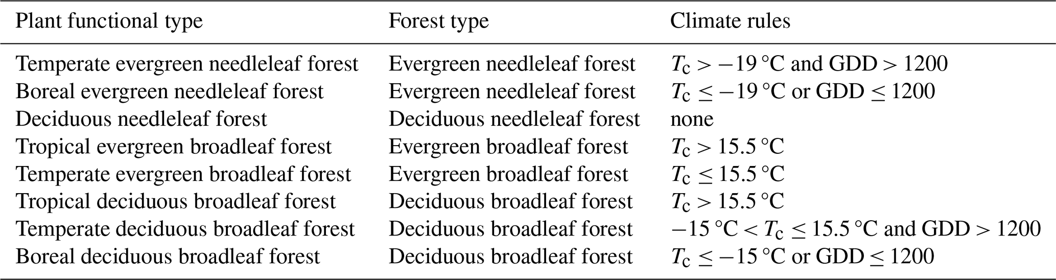
Table 3 Classification scheme for deriving plant functional types (PFTs) from forest life forms and climatic rules.

The previously generated consistency masks were then used to refine the classification within the needleleaf and broadleaf categories. This was achieved through a pixel-level comparison of type-specific consistency values. The process is illustrated below using the example of distinguishing the composition within needleleaf forests.

Comparisons are made among deciduous needleleaf forests (CON_DNF), evergreen needleleaf forests (CON_ENF), and mixed-leaf forests (CON_MF). If one value is the unique maximum, the pixel is classified as the corresponding type. However, if a tie for the maximum value exists (i.e., two or all three values are equal and maximal), the pixel is designated as “residual needleleaf forest” and reserved for subsequent processing.

The classification of evergreen and deciduous broadleaf forests (EBF and DBF) followed a procedure identical to that for needleleaf forests. This initial stage resulted in the annual classification of five primary PFTs (DNF, ENF, DBF, EBF, and MF), alongside a category of “residual” pixels requiring further processing. This category comprised pixels confirmed as either needleleaf or broadleaf, but for which a subtype could not yet be assigned. To resolve these pixels, two methods were subsequently employed: neighbourhood analysis and an environmental inference method.

Neighbourhood analysis: For each “residual” pixel, a 10 pixel × 10 pixel neighbourhood window was established, a size selected with reference to previous studies that performed neighbourhood analysis at similar scales (Harper et al., 2023). Within this window, the total number of pixels belonging to each of the five classified PFTs (DNF, ENF, DBF, EBF, and MF) was counted. The classification logic was then applied as follows:

For a “residual needleleaf pixel”, the counts of DNF, ENF, and MF neighbours were compared. Each pixel was classified based on the category with the maximum number of neighbours. If the counts for two or three types were equal (and maximal) or if no classified needleleaf neighbours existed within the window, the pixel was labelled as “pending”. Identical logic was applied to “residual broadleaf” pixels, on the basis of the counts of their DBF and EBF neighbours.

Environmental inference method: For the small number of remaining “pending” pixels (typically those with no classified neighbours), an environmental inference method was used to assign a final subtype on the basis of climatic and topographic data (see Sect. 2.4). The procedure involved the following steps: First, the climate zone and topography data were overlaid to create a map of unique “environmental strata” (i.e., unique combinations of climate and topography). Second, for each province and year, the relative proportion of the five PFTs was calculated within each unique environmental stratum. Third, a “pending” needleleaf pixel was assigned to the subtype that was most prevalent within its specific environmental stratum, according to the calculated proportions. The same logic was applied to “pending” broadleaf pixels.

Finally, the classifications from all the steps were merged to produce annual distribution maps for the five PFTs (DNF, ENF, DBF, EBF, and MF) for each province.

3.4.3 Final PFT classification

By adopting the methodology of Bonan et al. (2002) and utilising historical climate data (see Sect. 2.4), the five preliminary forest types were further subdivided into nine final PFTs. The specific climatic variables used for this classification are detailed in Table 3 and include the following:

T_c is the mean temperature in the coldest month.

GDD (Growing degree days) the days on which the annual cumulative temperature exceeds the 5 °C baselines.

The daily growing degree days (GDD_d) are calculated as shown in Eq. (4):

$$\begin{array}{}\text{(4)}& \mathrm{GDD}={\sum }_{d=\mathrm{1}}^{\mathrm{365}}\text{max}(T_{\mathrm{d}}-T_{\mathrm{b}},\mathrm{0})\end{array}$$

where T_d is the mean daily temperature and T_b is the base temperature for growth, which is set at 5 °C.

Since we used the monthly mean temperature data from 1981–2023 published by Peng et al. (2019a), an alternative method was employed to estimate GDD. This involved substituting the monthly mean temperature for T_d in Eq. (4) and then multiplying the result by the number of days in that month to yield a monthly GDD value. The annual GDD was subsequently calculated as the sum of these monthly values. We utilised the annual GDD and T_c values for each year during the 1981–2023 period to reflect the year-to-year dynamic changes in climatic conditions.

Through the sequence of methods detailed above, a comprehensive historical dataset of forest cover for China, classified on the basis of PFT, was produced.

3.5 Accuracy assessment

To validate the accuracy of our reconstructed annual PFT maps, we collected an extensive validation dataset covering the entire study area. Our validation samples were labelled on the basis of three data sources: (1) ground plots from the NFI conducted between 2009 and 2013. For each plot, the dataset provides the plot ID, geographic coordinates, and a classification into one of five forest types: ENF, EBF, DNF, DBF, and MF. (2) A collection of Landsat images spanning 1985–2023 (Cai et al., 2025) and (3) high-resolution imagery from Google Earth. First, to assess the temporal consistency of the NFI ground plots, we applied the normalised burn ratio (NBR) (García and Caselles, 1991) to the dense Landsat time series at these plot locations. The NBR is calculated as follows: ($\mathrm{NIR}-\mathrm{SWIR})/(\mathrm{NIR}+\mathrm{SWIR}$). This index is recognised for its sensitivity in detecting forest disturbances within Landsat time series (Perbet et al., 2024; White et al., 2022). We then employed the Landsat-based detection of trends in disturbance and recovery (LandTrendr) algorithm (Kennedy et al., 2010) to assess the stability of the 1 km grid cells surrounding these nationwide plots from 1985 to 2023. LandTrendr is a widely used disturbance detection method designed to detect anomalies and trends in time series, distinguishing between abrupt and gradual changes (Kennedy et al., 2018; Cheng et al., 2024). We implemented this algorithm in the GEE to distinguish between stable (remained unchanged between 1985 and 2023) and unstable (underwent a change in at least one year from 1985–2023) samples among the NFI ground plots and to identify the timing of any detected changes. This process yielded 5481 stable and 1229 unstable plots.

For unstable plots, we employed a cross-validation strategy to pinpoint the precise timing of land cover transitions. Specifically, we integrated raw NBR values derived from Landsat time series, LandTrendr-fitted temporal trajectories, and historical high-resolution imagery from Google Earth. We paid particular attention to validating the image features corresponding to the segments with the greatest magnitude of change between fitted vertices (Figs. S8 and S9). Through visual interpretation of spectral variations and textural features in the Google Earth imagery, we identified the exact year of land cover conversion (e.g., forestland converted to nonforest in 2013; Fig. S8). Consequently, the specific PFT label for each plot was consistently applied to all years within the 1985–2023 period where the plot was identified as forestland.

For the 1981–1984 period, we extrapolated the classification status from 1985 to the preceding years (i.e., plots identified as a specific forest PFT or nonforest in 1985 were assigned the same attribute for 1981–1984). This approach assumes that reversals between forest and nonforest states (e.g., forest–nonforest–forest transitions) are unlikely to occur within a 5 year window. The labelling was conducted by ten experts experienced in remote sensing data analysis. To ensure rigorous quality control, the samples with ambiguous features were subjected to team discussion, and the final reference labels were assigned only after a majority consensus. Finally, by integrating the annual records from both stable and unstable plots, we constructed a validation database spanning the entire 1981–2023 period.

Following the good practice guidelines for sample size decisions proposed by Olofsson et al. (2014), we used a proportional stratified sampling design to randomly draw validation samples from the validation database for each year, stratified on the basis of the five PFT classes: ENF, EBF, DNF, DBF, and MF. Each annual validation set consisted of approximately 1280 samples. For the proportionally rare classes (DNF and MF), the sample size was increased to 100 samples (Fig. S10) to reduce the standard error of the accuracy estimates for these less common categories. The PFT class of each sample was further confirmed following the same visual interpretation protocol described above. On the basis of these validation samples, we generated a confusion matrix for each year and calculated the producer's accuracy (PA), user's accuracy (UA), overall accuracy (OA), and F₁-score:

$$\begin{array}{}\text{(5)}& {\displaystyle }& {\displaystyle }{\text{PA}}_k={\displaystyle \frac{p_{kk}}{{\sum }_{j=\mathrm{1}}^m{p}_{kj}}}\text{(6)}& {\displaystyle }& {\displaystyle }{\text{UA}}_k={\displaystyle \frac{p_{kk}}{{\sum }_{i=\mathrm{1}}^m{p}_{ik}}}\text{(7)}& {\displaystyle }& {\displaystyle }\text{OA}={\sum }_{k=\mathrm{1}}^m{p}_{kk}\end{array}$$

$$\begin{array}{}\text{(8)}& F_{\mathrm{1}}={\displaystyle \frac{\mathrm{2}\times \text{PA}\times \text{UA}}{\text{PA}+\text{UA}}}\times \mathrm{100}\mathit{\%}\end{array}$$

where p_kk is the area proportion of class k that is correctly classified (i.e., class k in both the reference data and the map); ${\sum }_{j=\mathrm{1}}^m{p}_{kj}$ represents the total area proportion of class k in the reference data (the row sum), ${\sum }_{i=\mathrm{1}}^m{p}_{ik}$ represents the total area proportion of class k in the classified map (the column sum), and m is the number of land cover types. We then corrected the accuracy estimates on the basis of map uncertainties and calculated the corresponding standard errors and 95 % confidence intervals (Olofsson et al., 2014). We also conducted cross-validation with existing annual land cover products (ESA CCI, MCD12Q1, and GLC_FCS30D), which included five PFT classes (ENF, EBF, DNF, DBF, and MF) to comprehensively evaluate the quality of the dataset reconstructed in this study.

In addition to this sample-based validation, an indirect accuracy assessment was performed by analysing the consistency among the input LULC datasets. This approach is pertinent as the final product is an integration of information from these sources. Here, consistency is defined at the pixel level as the number of LULC datasets with the same classification of a specific forest type. The underlying assumption of this analysis is that a high consistency value for a given pixel indicates high confidence in its classification and a high likelihood of it being correct (Xia et al., 2023).

3.6 Forest change analysis

Forest change is defined as the transition in land cover between forestland and nonforest states over a given period. This type of change is typically classified into change events (i.e., forest gain or loss) and stable states (i.e., persistent forest or persistent nonforest) (Winkler et al., 2021). Forest gain represents a transition from a nonforest state to a forest state, whereas forest loss is the reverse process (Hansen et al., 2013). To identify the onset year and duration of forest change events across China for the period 1981–2023, a pixel-level time series analysis was developed on the basis of the annual forest mask sequence.

This methodology is illustrated here using the detection of forest gain. First, the annual forest masks were standardised to binary values (0 = nonforest; 1 = forest) to create a spatiotemporal data cube. For this analysis, a “stable” forest state was defined as a pixel remaining as forestland for at least five consecutive years. The onset year of a forest gain event was then identified for each pixel as the first year it transitioned from a nonforest state to a stable forest state.

Following the identification of a gain event, the duration of forest persistence was calculated. This duration is the number of years from the onset of the gain until either (a) the pixel underwent a stable loss event, defined as transitioning to nonforest and remaining so for at least five consecutive years, or (b) the end of the study period (2023) if no such loss event occurred. The detection of forest loss events and their duration was based on the inverse logic.

This analysis produced four maps: two indicating the onset year for forest gain and loss events and two representing the durations of these respective periods.

3.7 Modelling assessment using LPJ–GUESS

The impact of the new PFT distribution on surface fluxes was assessed using LPJ–GUESS (Lindeskog et al., 2021), a process-based DGVM. The model was driven with Chinese meteorological forcing data (CMFD 2.0) (He et al., 2020) at a 0.1° resolution for the period of 1951–2023, this dataset included daily averages of temperature, incoming shortwave radiation, and precipitation. The data are publicly available from the National Tibetan Plateau Data Center at https://doi.org/10.11888/Atmos.tpdc.302088 (He et al., 2024b). Atmospheric CO₂ concentrations followed historical trajectories (Friedlingstein et al., 2025). Gridded monthly nitrogen deposition data (0.5° resolution) were also used as inputs (Lamarque et al., 2013), using the nearest grid cell value for each simulation grid. Soil properties – namely, the fractions of sand, silt, and clay; organic carbon content; C:N ratio; pH; bulk density; and organic carbon density – were derived from the China dataset of soil properties for land surface modelling version 2 (CSDL v2) dataset (Shi et al., 2025). This database, generated using advanced integrated machine learning algorithms from multiple representative historical soil profiles and high-resolution environmental covariates, provides 0.1° maps of six soil layers across China. The data are publicly available at https://www.scidb.cn/s/ZZJzAz (last access: 23 September 2025). We averaged the soil texture data from 0–200 cm and resampled all the soil inputs to align them with the meteorological forcing grid.

The LPJ-GUESS model was run at a 0.1° × 0.1° spatial resolution. Vegetation structure and its associated carbon, water, and nitrogen pools were initialised using a 500 year spin-up phase (starting from bare ground) by cycling 1951–1980 detrended meteorological data. This was followed by a historical simulation from 1981–2023. To account for natural disturbances, a disturbance interval of 100 years was established, and the GlobFirm wildfire submodel (Thonicke et al., 2001) was used. To ensure the ability of the model to simulate Chinese forest ecosystems, key parameters related to photosynthesis, autotrophic respiration, and plant water use efficiency were manually adjusted after benchmarking (all the updated PFT parameters are summarized in Table S2).

To isolate and quantify the independent impact of the PFT distribution, we designed three distinct model experiments. During the 1981–2023 period, all three experiments were driven by the same climate forcing data and consistent model parameters. The only difference among the experiments was the PFT input map: EXP1 utilised the new PFT map developed in this study, EXP2 utilised the global PFT dataset from ESA CCI (Harper et al., 2023), and EXP3 utilised the global PFT dataset from MCD12Q1 (Sulla-Menashe et al., 2019). In all three experiments, we cycled the 2010 PFT distribution to maintain a static land cover driver. We simulated the monthly total GPP, NEE, LAI, and ET for 2010, focusing our comparison on the mean differences between the PFT datasets during the summer (June–August) to highlight primary changes. As the PFT distribution map was the sole variable altered between experiments, any observed differences in the output fluxes could be directly attributed to its influence. To assess the plausibility of these changes, the simulation results were also compared to four remote sensing and observation-based products: FLUXCOM GPP, FLUXCOM NEE, GIMMS LAI4g, and GLEAM ET. All the observational products were resampled to a 0.1° resolution using bilinear interpolation to match the LPJ–GUESS simulation grid.

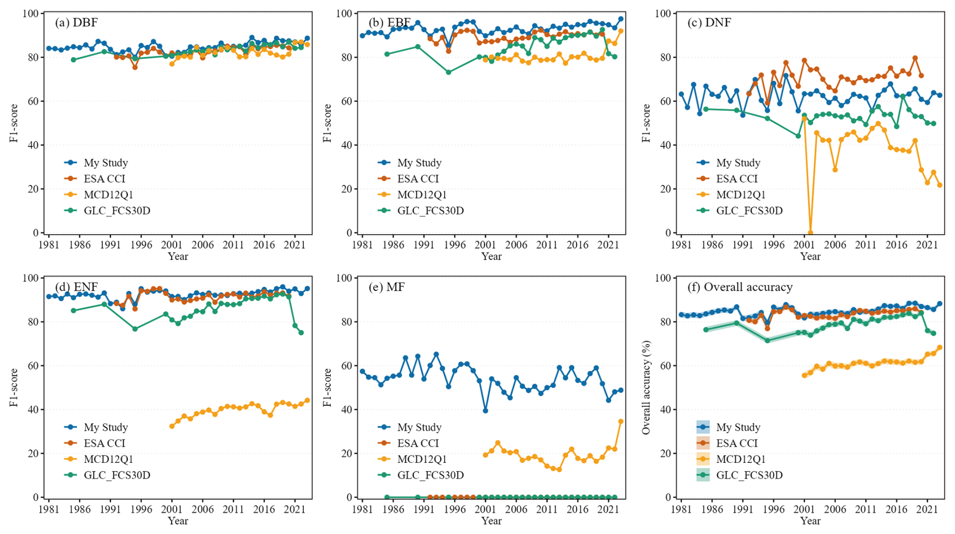
Figure 2 F₁ scores and overall accuracies (OAs) for our dataset (this study), the European Space Agency Climate Change Initiative land cover (ESA CCI) dataset, the Moderate Resolution Imaging Spectroradiometer land cover (MCD12Q1) dataset, and the global 30 m land-cover dynamics monitoring dataset (GLC_FCS30D), which were validated against national forest inventory (NFI) field plots. The shaded area in (f) represents ± 1  standard error.

4 Results

4.1 Accuracy assessment of the reconstructed PFT dataset

Independent validation based on five forest types for the period 1981–2023 demonstrates that the accuracy of the PFT dataset reconstructed in this study is both stable and satisfactory. The OA ranged from 79.74 % to 88.5 %, with a mean OA of 84.86 % ± 1.18 % (Fig. 2f). Among the specific forest classes, the highest mean F₁ score was achieved for EBF (93.03 %), followed by the ENF (92.49 %), DBF (84.89 %), DNF (62.29 %), and MF (54.03 %) classes (Fig. 2a–e). Furthermore, in most years, the overall accuracy of our dataset (mean 84.86 % ± 1.18 %) was greater than that of ESA CCI (mean 83.47 % ± 1.15 %), MCD12Q1 (mean 61.17 % ± 1.36 %), and the global 30 m land-cover dynamics monitoring dataset (GLC_FCS30D) (mean 78.92 % ± 1.24 %) (Fig. 2f). For the classes with large areal proportions, such as DBF, EBF, and ENF, the F₁ scores for our dataset also demonstrated superior and more stable performance than ESA CCI, MCD12Q1, and GLC_FCS30D did (Fig. 2a–e). This independent validation confirms the high spatial accuracy of the reconstructed PFT data in comparison to prominent existing datasets. Moreover, the temporal coverage of the dataset reconstructed in this study spans 43 years (1981–2023), exceeding that of ESA CCI (1992–2020), MCD12Q1 (2001–2023), and GLC_FCS30D (1985–2022). Analysis of the consistency between our reconstructed PFT dataset and the input LULC datasets revealed that the reconstructed broadleaf forests were more consistent than the needleleaf forests were (Fig. S5b–f), indicating greater confidence in the reconstructed BF results. Among the five PFTs, the confidence ranking from highest to lowest was DBF, EBF, ENF, DNF, and MF (Fig. S5b–f). Furthermore, according to our methodology, a pixel-weighted average over the 1981–2023 period indicates that fewer than 1 % of the pixels for all five reconstructed PFTs did not fall within their corresponding consistency type classes (the specific proportions were 0.50 % for DBF, 0.10 % for EBF, 0.03 % for DNF, 0.01 % for ENF, and 0.05 % for MF, Fig. S11).

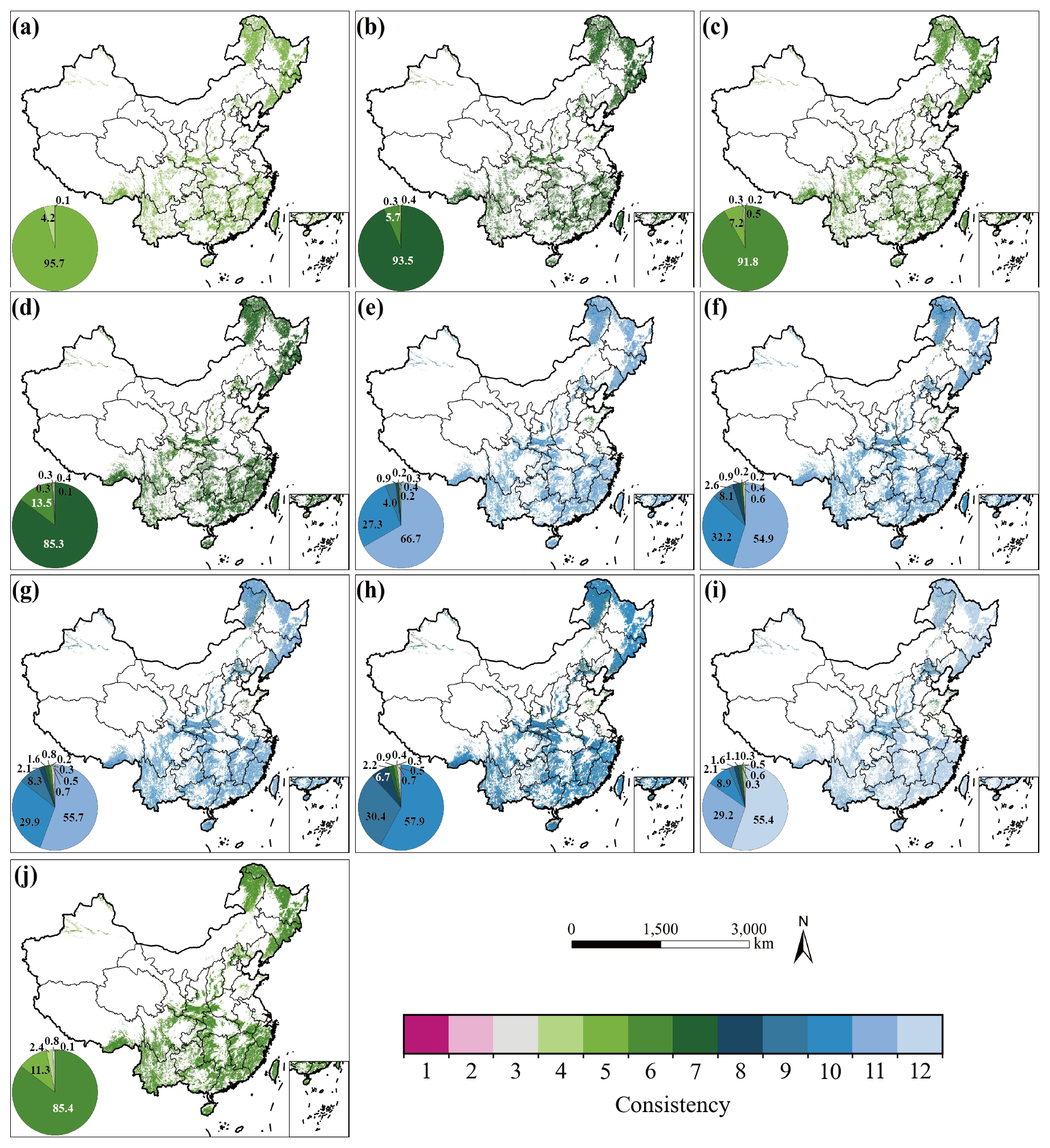
Figure 3 The spatial distribution of reconstructed forest cover is presented at 5 year intervals from 1981–2023 (a) 1981, (b) 1985, (c) 1990, (d) 1995, (e) 2000, (f) 2005, (g) 2010, (h) 2015, (i) 2020, and (j) 2023, along with corresponding cross-product consistency scores. The reconstruction for each time point was compared against an ensemble of data products sourced externally (n = 5, 7, 6, 7, 11, 11, 11, 10, 12, and 6). The inset pie chart (lower left) quantifies the areal proportion of the reconstructed forest dataset at various consistency levels, which serves as a proxy for the confidence in the resulting maps.

The internal consistency of the reconstructed total forest cover was assessed at ten specific time points: 1981, 1985, 1990, 1995, 2000, 2005, 2010, 2015, 2020, and 2023 (Fig. 3). The number of inputs LULC datasets available for reconstruction varied at each time point, with 5, 7, 6, 7, 11, 11, 11, 10, 12, and 6 products used for each respective year. The analysis revealed that for each of the ten time points, the maximum possible consistency score was achieved for 95.7 %, 93.5 %, 91.8 %, 85.3 %, 66.7 %, 54.9 %, 55.7 %, 57.9 %, 55.4 %, and 85.4 % of the reconstructed forestland pixels, respectively. Conversely, pixels with the lowest possible consistency (CON = 1) consistently accounted for a small fraction of the total reconstructed forest area, ranging from 0 % to 0.26 % across different years (Fig. 3). Spatially, areas with lower forest consistency were predominantly located in the arid and semiarid regions of northwestern China (e.g., Ningxia) and the highly fragmented landscapes of the eastern coastal plains (e.g., Tianjin, Shandong, Jiangsu, and Shanghai). In contrast, high-consistency forestland areas were concentrated mainly in regions with extensive and stable forest cover, primarily in southern and central China, including provinces such as Hubei, Zhejiang, Guangxi, Guizhou, Yunnan, and Jiangxi (Fig. S12). A comparison and an analysis of the NFI data with the forest area estimates reconstructed in this study at the provincial scale (Fig. S13) reveal a good match for multiple years (1981–2023), with an R² close to 1 and a p-value < 0.001. These findings indicate that the reconstructed data from this study are highly consistent with the NFI statistics in terms of overall trends.

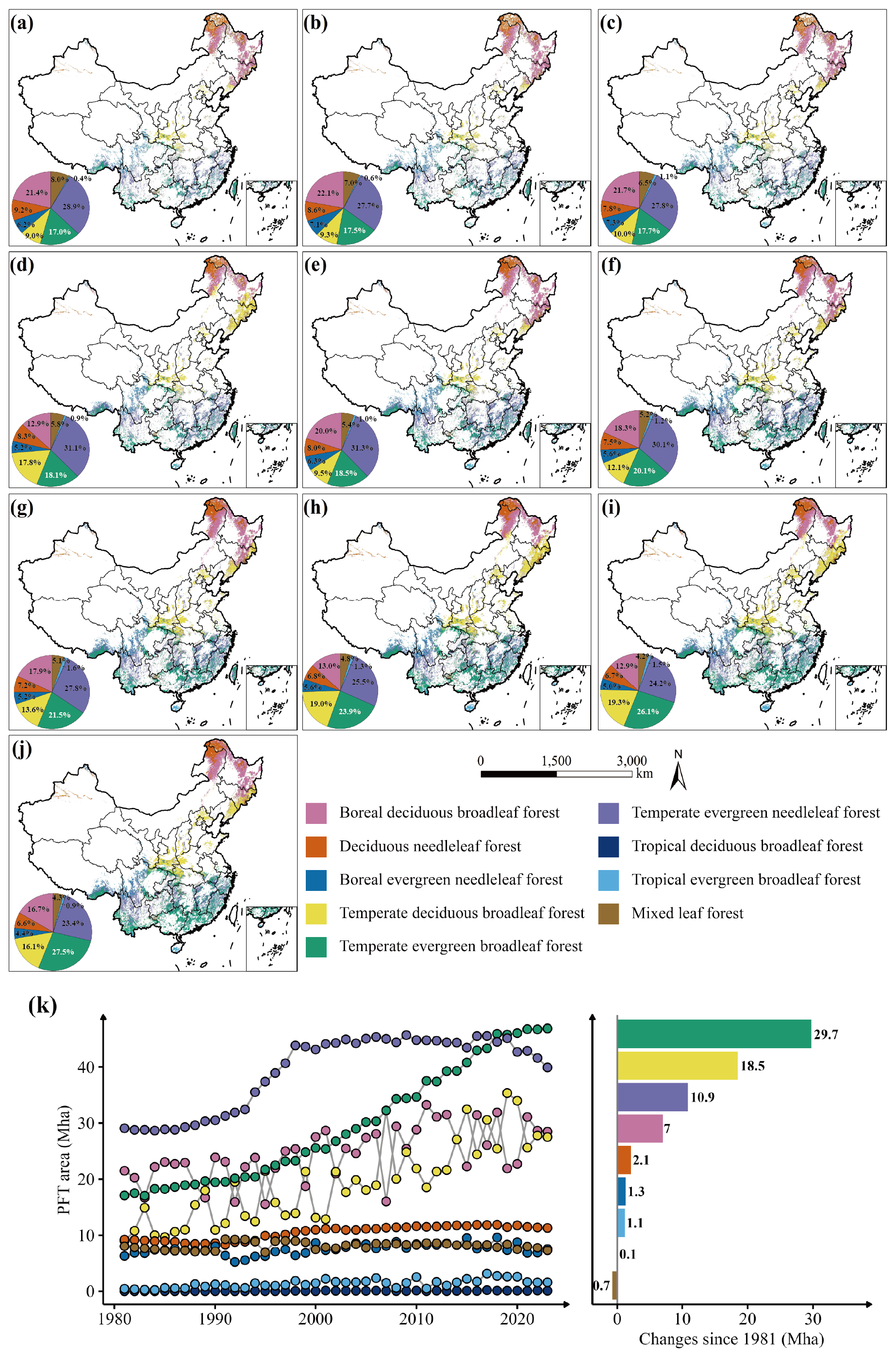
Figure 4 Spatial distribution patterns and area proportions of China's forest plant functional types (PFTs) for selected years between 1981 and 2023; (a–j) correspond to 1981, 1985, 1990, 1995, 2000, 2005, 2010, 2015, 2020, and 2023, respectively; (k) Temporal dynamics and total variation in PFTs from 1981 to 2023. Note: PFTs were not reconstructed for Hong Kong, Macau, and Taiwan (post-2013) due to the absence of statistical data and their exclusion from national afforestation programs.

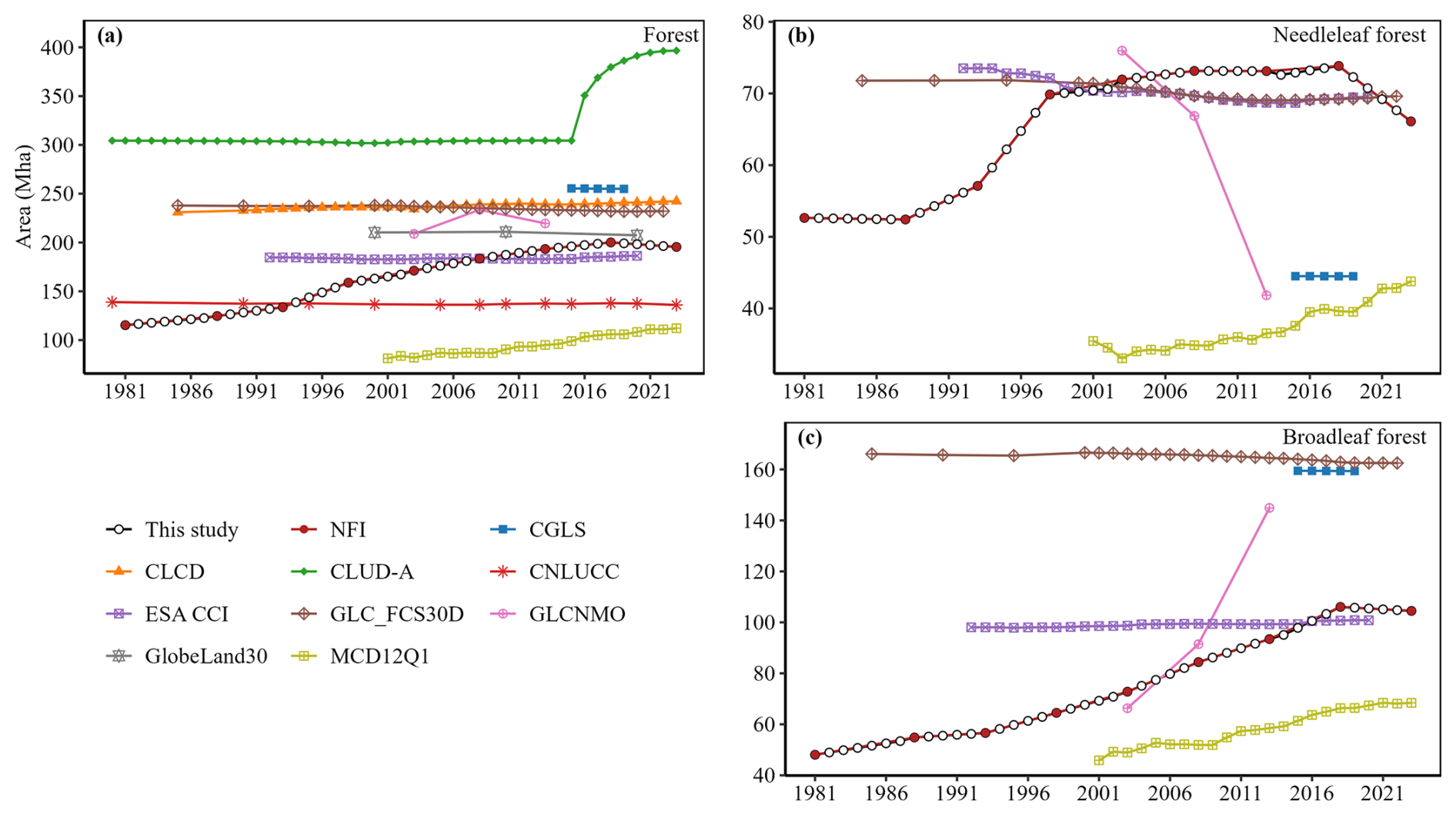
Figure 5 Temporal dynamics of the national-scale total forestland area, with the results of this study compared with data from the national forest inventory (NFI) and other selected land use and land cover (LULC) products: (a) forestland, (b) needleleaf forest, and (c) broadleaf forest.

4.2 Spatiotemporal distribution of the reconstructed PFT dataset

This dataset provides the annual forest cover distribution from 1981 to 2023 (Fig. 3) and the distribution of nine PFTs at a 1 km spatial resolution (Fig. 4). The data are supplied in the WGS 1984 Albers equal-area conic projection. The nine PFTs are (1) boreal evergreen needleleaf forest, (2) temperate evergreen needleleaf forest, (3) temperate evergreen broadleaf forest, (4) boreal deciduous broadleaf forest, (5) temperate deciduous broadleaf forest, (6) tropical deciduous broadleaf forest, (7) tropical evergreen broadleaf forest, (8) deciduous needleleaf forest, and (9) mixed leaf forest.

For the reference year 2023, the dataset indicates that China's forests are composed of temperate evergreen broadleaf forest (27.5 %), temperate evergreen needleleaf forest (23.4 %), boreal deciduous broadleaf forest (16.7 %), temperate deciduous broadleaf forest (16.1 %), deciduous needleleaf forest (6.6 %), boreal evergreen needleleaf forest (4.4 %), mixed leaf forest (4.3 %), tropical evergreen broadleaf forest (0.9 %), and tropical deciduous broadleaf forest (0.05 %). Although temperate evergreen needleleaf forests and boreal deciduous broadleaf forests were the two largest components by area prior to 2000, their proportional contributions to the total forest area subsequently declined from 31.3 % to 23.4 % and from 20.0 % to 16.7 %, respectively. Conversely, the proportional representation of temperate evergreen broadleaf and temperate deciduous broadleaf forests expanded, increasing from 18.5 % to 27.5 % and from 9.5 % to 16.1 %, respectively (Fig. 4).

Spatially, the primary forest regions are concentrated in Northeast, Southeast, and Southwest China, whereas forest cover is relatively sparse in Northwest, Central, and East China. Furthermore, evergreen needleleaf and evergreen broadleaf forests are predominantly distributed across southern China. Deciduous needleleaf forests are concentrated in the Greater Khingan Range in the northernmost part of Northeast China, while deciduous broadleaf forests are located mainly in Northeast China and the Qinling Mountains of Central China.

With respect to its temporal evolution, our reconstructed forest dataset faithfully reproduces the long-term dynamics of forest cover in China (Fig. 5). According to statistics from the NFI, China's forest cover has a mean annual growth rate of 1.75 %. The reconstructed forest cover dataset reveals a substantial increase in China's total forest area from 115.28 million  ha (Mha) in 1981 to 195.45 Mha in 2023, with a peak of 200.05 Mha observed in 2018 (Fig. 5a). This represents an annualised growth rate of 1.50 %, demonstrating strong agreement with this national benchmark. Furthermore, our dataset accurately captures the distinct historical trajectories of two principal forest categories – broadleaf and needleleaf forests – since the 1980s (Fig. 5b and c). This net increase was primarily propelled by the expansion of temperate and boreal forests (Fig. 4). For example, the area of temperate evergreen broadleaf forest more than doubled between 1981 and 2023, increasing from 17.10 to 46.85 Mha (Fig. 4k). During this period, significant areal gains were also recorded for temperate deciduous broadleaf, temperate evergreen needleleaf, and boreal deciduous broadleaf forests. In contrast, absolute changes in the extent of tropical PFTs, boreal evergreen needleleaf forests, and mixed leaf forests were minimal over the same interval (Fig. 4k).

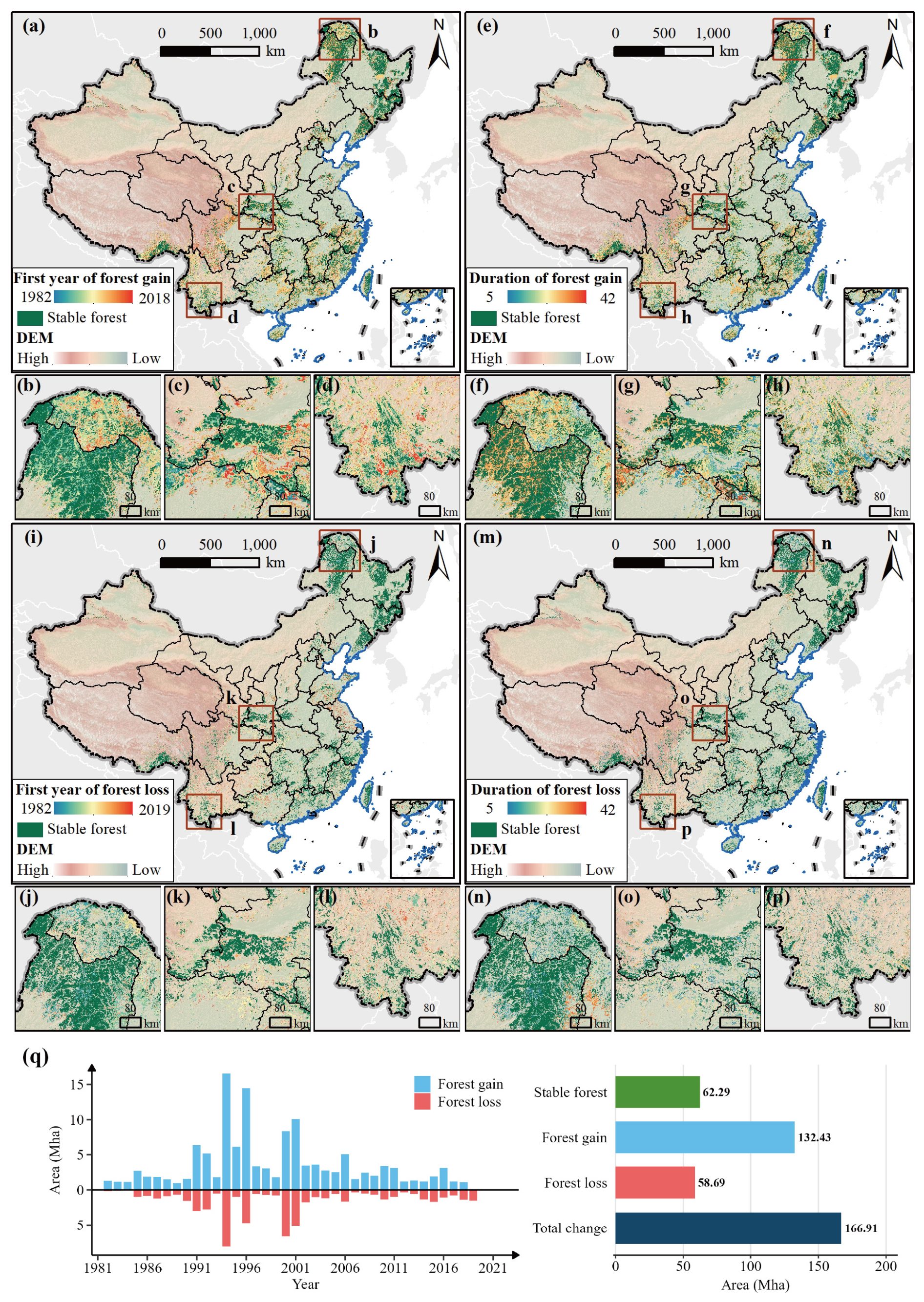
Figure 6 Spatiotemporal dynamics of forest gain and loss in China from 1981 to 2023. This figure presents: (a–h) the spatial patterns of forest gain, showing the onset year and duration; (i–p) the spatial patterns of forest loss; and (q) the national-scale temporal dynamics, including the annual areas of forest gain and loss and a summary of total stable, gained, and lost forest areas.

4.3 Spatiotemporal patterns of forest cover change in China

Between 1981 and 2023, the total area experiencing forest change (gross change) was 166.91 million  ha (Mha), which is equivalent to approximately 17 % of China's terrestrial surface. This comprised 132.43 Mha of forest gain (14 % of the national land area) and 58.69 Mha of forest loss (6 % of the national land area). Forests that remained stable, persisting from 1981 to 2023, covered 62.29 Mha. This stable area represents 54 % of the total forest extent in 1981, implying that the remaining 46 % of the original 1981 forest cover underwent some form of change during the study period (Fig. 6q). We observed a prevalent pattern of forest change across several regions of China, characterised by a progression from more accessible areas (i.e., lower elevations near roads) to more remote locations (i.e., higher elevations far from roads). This dynamic often manifested as a core-to-edge expansion of existing forest patches (Fig. 6a–p). We detected severe forest loss on the eastern Qinghai-Tibet Plateau from 1990–1996, which appeared to be driven primarily by commercial logging (Chen et al., 2013). Following the implementation of large-scale ecological restoration programmes initiated in 1998 – specifically, the Natural Forest Protection Programme and the Grain for Green Programme – forest cover exhibited a recovery trend from 2000 to 2008 (Liu et al., 2008). Temporally, both forest loss and gain were continuous dynamic processes throughout the entire period. A prominent peak in forest turnover occurred between 1991 and 1996, culminating in 1994 when the combined area of gain and loss surpassed 24.63 Mha. After 2001, both gain and loss areas exhibited a general downwards trend, albeit with notable fluctuations, and moderate recessions in turnover were observed in approximately 2006, 2010, and 2016. Furthermore, forest loss and gain events tended to occur relatively concurrently (Fig. 6q).

Our analysis revealed that forest loss events are typically short in duration (Fig. S14). More than 30 % of all observed losses persisted for only 5–9 years. In contrast, forest gain is characterised by substantially longer persistence, with a modal duration of 25–29 years. This highlights the long-term stability of large tracts of newly established forests. The statistical distributions of persistence durations for forest gain and loss are markedly different. Loss events are predominantly concentrated in the shorter-duration intervals, whereas periods of gain are more concentrated in the medium- to long-duration brackets. This divergence indicates that newly established forests tend towards greater stability and longevity, whereas forest loss manifests as a more fragmented and ephemeral phenomenon.

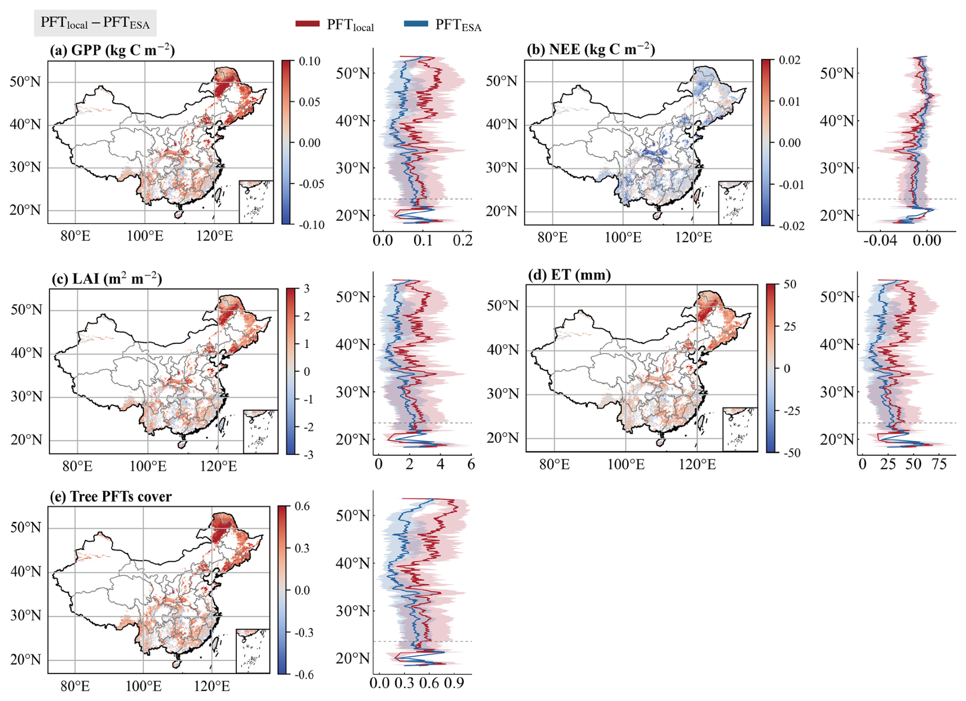
Figure 7 Comparison of Lund–Potsdam–Jena general ecosystem simulator (LPJ–GUESS) model simulations (a–d) and their underlying plant functional type (PFT) forcing data (e) for the summer of 2010. Comparisons are made between the PFT product reconstructed in this study (PFT_local) and the global PFT map from the European Space Agency (PFT_ESA). The first four panels (a–d) show differences in the simulated gross primary productivity (GPP), net ecosystem exchange (NEE), leaf area index (LAI), and actual evapotranspiration (ET). Panel (e) shows differences in tree PFT cover derived directly from the input PFT maps. For all panels, the maps display the spatial difference (PFT_local−PFT_ESA), while the plots show the zonal mean and standard deviation for the PFT_local (red) and PFT_ESA (blue) datasets individually. Note that the data in panels (a–d) are model outputs, whereas the data in panel (e) are from the input maps.

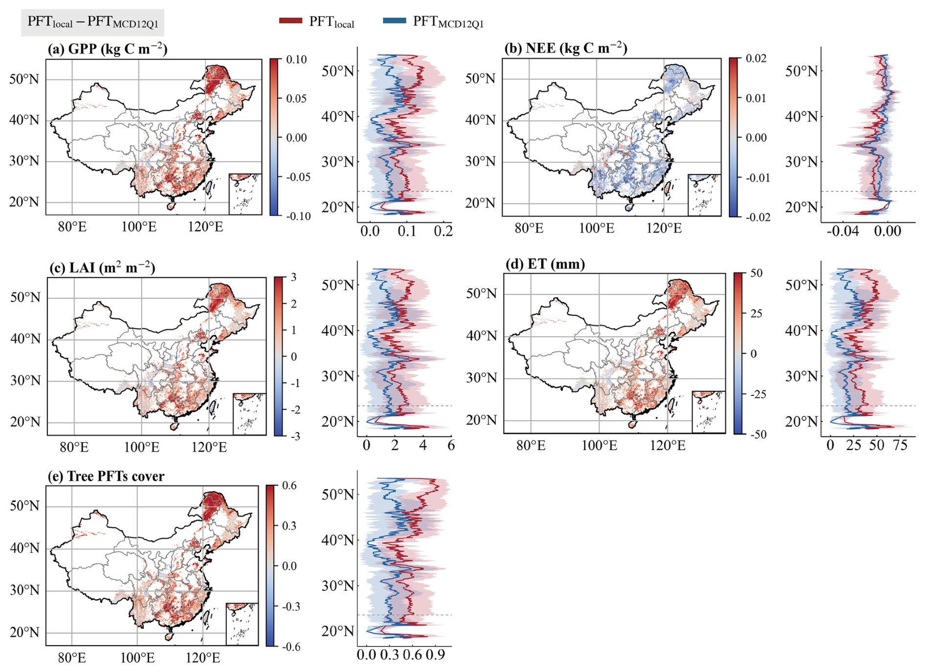
Figure 8 Comparison of Lund–Potsdam–Jena general ecosystem simulator (LPJ–GUESS) model simulations (a–d) and their underlying plant functional type (PFT) forcing data (e) for the summer 2010. Comparisons are made between the PFT product reconstructed in this study (PFT_local) and the global PFT map from the MODIS land cover type product (PFT_MCD12Q1). The first four panels (a–d) show differences in the simulated gross primary productivity (GPP), net ecosystem exchange (NEE), leaf area index (LAI), and actual evapotranspiration (ET). Panel (e) shows differences in tree PFT cover derived directly from the input PFT maps. For all panels, the maps display the spatial difference (PFT_local−PFT_MCD12Q1), while the plots show the zonal mean and standard deviation for the PFT_local (red) and PFT_MCD12Q1 (blue) datasets individually. Note that the data in panels (a–d) are model outputs, whereas the data in panel (e) are from the input maps.

4.4 LPJ–GUESS simulations: comparing the reconstructed PFT dataset to ESA CCI and MCD12Q1

We assessed the impact of different PFT forcing datasets on ecosystem simulations by comparing outputs from the LPJ–GUESS model driven with our reconstructed PFT product (hereafter PFT_local) versus the global PFT map (PFT_global) from the European Space Agency (hereafter PFT_ESA) and the MCD12Q1 product (hereafter PFT_MCD12Q1). The analysis, exemplified using data for the year 2010, quantifies the resulting differences in key ecosystem variables: GPP, NEE, LAI, and ET (Fig. 7). Here, we focus on the mean differences (PFT_local minus PFT_global) during the summer period (June–August) to highlight the primary impacts. The results indicate that the most marked differences in the simulated carbon and water fluxes spatially coincide with regions where the three products show substantial differences in the fractional coverage of tree PFTs. Regions with a higher tree cover fraction in the PFT_local dataset than in the PFT_ESA dataset, particularly in northeastern China (Fig. 7e, red), exhibit correspondingly elevated GPP, LAI, and ET, along with a diminished NEE. Consequently, the resulting differentials are positive for the former variables and negative for NEE. Conversely, where the PFT_ESA dataset indicates greater tree coverage, such as in parts of southwestern China (Fig. 7e, blue), these relationships are inverted. Similarly, the comparison with PFT_MCD12Q1 yields analogous results (Fig. 8).

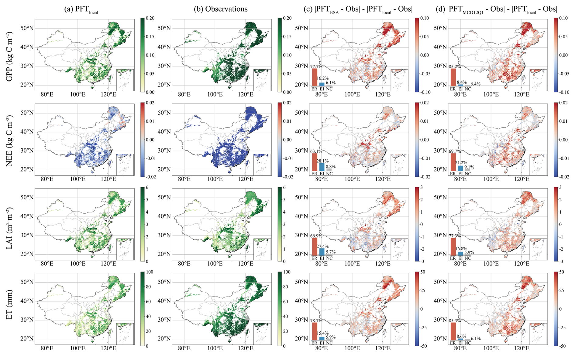
Figure 9 Model data comparison for gross primary productivity (GPP), net ecosystem exchange (NEE), the leaf area index (LAI), and actual evapotranspiration (ET) for summer (June–August) 2010. (a) Ecosystem variables simulated by the Lund–Potsdam–Jena general ecosystem simulator (LPJ–GUESS) model using our reconstructed dataset (PFT_local). (b) Corresponding observation-based benchmark products from FLUXCOM (GPP, NEE), GIMMS (LAI4g), and GLEAM (ET). (c) The difference in absolute error between model runs, is used to quantify the difference in performance between our reconstructed dataset (PFT_local) and the European Space Agency dataset (PFT_ESA) relative to the remote sensing observation products (Obs), is calculated as $\mathrm{|}{\mathrm{PFT}}_{\mathrm{ESA}}-\mathrm{Obs}\mathrm{|}-\mathrm{|}{\mathrm{PFT}}_{\mathrm{local}}-\mathrm{Obs}\mathrm{|}$. (d) Same as (c) but quantifying the difference in performance against the MODIS land cover type product (PFT_MCD12Q1), which is calculated as $\mathrm{|}{\mathrm{PFT}}_{\mathrm{MCD}\mathrm{12}\mathrm{Q}\mathrm{1}}-\mathrm{Obs}\mathrm{|}-\mathrm{|}{\mathrm{PFT}}_{\mathrm{local}}-\mathrm{Obs}\mathrm{|}$. For both (c) and (d), positive values indicate that PFT_local reduces the simulation error (improves performance) compared with the global PFT datasets, whereas negative values indicate an increase in error (performance degradation), and the bar graph displays the percentages of error reduced (ER), increased (EI), and no change (NC).

To assess the realism of the simulations, we benchmarked the model outputs against a suite of remote sensing-based products (FLUXCOM GPP, FLUXCOM NEE, GIMMS LAI4g, and GLEAM ET), with all the datasets aggregated to a common 0.1° resolution (Fig. 9 for summer, June–August). In Fig. 9a and b, we first present a direct comparison between the surface fluxes simulated using our reconstructed PFT map (PFT_local) and the observed benchmarks. This baseline comparison highlights inherent discrepancies attributable to both structural biases in the LPJ–GUESS model and uncertainties within the remote sensing products themselves. Figure 9c and d then allow the impact of the PFT forcing to be isolated by showing the change in absolute simulation error relative to the observational data. Areas of improvement (demarcated in red) and degradation (in blue) in model performance when PFT_local is used in place of PFT_ESA and PFT_MCD12Q1 are explicitly mapped.

High simulated GPP values (> 0.2 kg C m⁻²) are concentrated in the forested regions of northeastern China (e.g., the Greater Khingan and Changbai Mountains), the central Qinling Mountains, and southeastern China. Conversely, low GPP values are characteristic of the arid and semiarid regions of the northwest and the Tibetan Plateau (Fig. 9a), where productivity is constrained by water availability and low temperatures. On a macroscale, the simulation accurately captures this geographical distribution. PFT_local demonstrates a distinct advantage in terms of PFT forcing. Compared with PFT_ESA, it reduces simulation errors across 77.7 % of the domain (Fig. 9c), with improvements primarily concentrated in Northeast China, North China, and the Qinling Mountains (red areas); conversely, areas of increased error (16.2 %) are sporadically distributed across southern China. The improvement is even more pronounced relative to PFT_MCD12Q1, for which error reductions cover 85.2 % of the terrestrial area, whereas increased errors are confined to only 8.4 % of the domain, specifically in Southwest China and Taiwan (Fig. 9d). With respect to the NEE simulations, PFT_local significantly outperforms PFT_ESA, with fewer errors across 63.1 % of the domain (Fig. 9c). The most pronounced improvements are observed in the Qinling Mountains (indicated by deep red), whereas areas of increased error (28.1 %, blue regions) are primarily concentrated in Northeast and Southwest China. Relative to PFT_MCD12Q1, the extent of improvement expands to 69.7 %, whereas the increase in error (21.2 %) is distributed mainly across the Northeast China, Southwest China, and Taiwan regions (Fig. 9d).

The simulated LAI exhibits a spatial pattern analogous to that of the GPP (Fig. 9a). Relative to PFT_ESA, PFT_local reduces errors across 66.9 % of the domain (marked in red in Fig. 9c), with the most pronounced improvements observed in the Northeast China and Qinling regions; conversely, areas of increased error (27.4 %, blue) are primarily situated in southern China. For PFT_MCD12Q1, the extent of error reduction expands to 77.3 %, while increased errors (16.8 %) are confined largely to Southwest China and Taiwan (Fig. 9d). The spatial pattern of the simulated ET is consistent with that of the other variables analysed (Fig. 9a). With respect to model improvement (Fig. 9c), PFT_local reduces simulation errors across 78.7 % of China relative to PFT_ESA (indicated by extensive red areas), except for certain parts of southern China. Compared with PFT_MCD12Q1, this proportion increases to 85.3 % (Fig. 9d). These results indicate that the reconstructed dataset demonstrates distinct superiority over the ESA and MCD12Q1 datasets in simulating major carbon and water fluxes across mainland China.

5 Discussion

In this study, a method to integrate the “top-down” spatial detail derived from multisource remote sensing products with the “bottom-up” statistical constraints provided by the NFI was developed. This approach not only overcomes the limitations of relying on single data sources but also rectifies a well-documented defect in existing land cover products: specifically, their frequent failure to adequately capture the extensive, policy-driven forest expansion trend in China since the 1980s, which leads to an underestimation of the forest cover growth rate (Fig. 5) (Yue et al., 2024; Zhu et al., 2025; Yu et al., 2022; Xia et al., 2023). Furthermore, existing LULC products cannot be used to accurately resolve the historical trajectories of needleleaf and broadleaf forest differentiation. Consequently, the DGVMs driven by these historical datasets may severely underestimate China's carbon sink potential. We tested the hypothesis that a more accurate vegetation cover map would improve land surface model performance by using our reconstructed PFT map to drive the LPJ–GUESS dynamic vegetation model. The results indicate that compared with using the ESA CCI and MODIS global PFT datasets in simulations, our dataset significantly improved the simulation accuracy of key ecosystem variables (Fig. 9). The spatial patterns of these improvements coincide strongly with regions where the tree cover in our dataset differs most from that in global products, particularly in Northeast China (Figs. 7 and 8). This provides compelling evidence for the critical role of accurate vegetation representation in simulating carbon and water cycles. By providing a more precise depiction of historical forest dynamics, this dataset offers improved constraints for the model parameterisation of surface albedo, canopy structure, and transpiration, thereby enabling more robust flux estimates.

Notably, while both this study and that of Xia et al. (2023) aimed to reconstruct forest growth trends consistent with NFI records, certain discrepancies exist in the results. For instance, Xia et al. (2023) reported low forest classification consistency primarily in the northwestern regions of Xinjiang, Qinghai, and Ningxia, whereas our study revealed low consistency solely in Ningxia. This divergence likely stems from our adoption of stricter NFI area constraints specifically, utilising “wooded land” (excluding shrubland) rather than total forestland area. By excluding shrublands, our extracted distribution of “potential forest” aligns more closely with the core forest distribution in regions such as Xinjiang and Qinghai. Furthermore, a comparison of data between 1990 and 1995 by Xia et al. (2023) suggested a relatively low area of forest loss in China during this period. In contrast, our dataset reveals the opposite trend, identifying a peak in forest loss between 1991 and 1994. This difference is likely attributable to the annual temporal resolution of our dataset, which offers heightened sensitivity to forest gain and loss events. Finally, our dataset provides a comprehensive annual time series of nine distinct forest PFTs spanning the period 1981–2023. It is therefore necessary to utilise this newly developed and validated dataset to systematically re-evaluate the impacts of forest cover change on terrestrial ecosystems in China.

However, this study is subject to certain uncertainties and limitations that need to be addressed in future work. First, as an integrated data product, our dataset inherits uncertainties from its primary sources: the input LULC data and the NFI statistics. Most satellite-based LULC datasets rely on machine learning classifiers, the accuracy of which is contingent upon the representativeness, quantity, and quality of training samples. Furthermore, our dataset's accuracy is substantially dependent on the NFI data, which has distinct uncertainties stemming from inventory methodologies and the representativeness of ground plots. Notably, the precision of NFI data has improved over time because of the progressive evolution of its sampling design; for example, the introduction of combined ground-truth and remote sensing samples for the fourth NFI (1989–1993) and a significant increase in remote sensing samples since the sixth NFI (1999–2003) markedly enhanced its accuracy (Lei et al., 2009). Consequently, any uncertainty within the NFI data inevitably propagates into our reconstructed dataset.

Second, our method employs a 1 km binary classification scheme. This approach may induce scale aggregation effects in arid and semiarid regions where forest cover is naturally sparse and fragmented. Specifically, dispersed forest pixels risk being omitted if they do not constitute the dominant land cover within a 1 km grid cell. While incorporating shrublands might capture the spectral signatures of these sparse pixels, we strictly excluded them due to the fundamental biophysical disparities between shrubs and trees – namely in carbon allocation, allometric scaling, and biomass turnover (Verbruggen et al., 2021). This distinction is critical given the vast distribution of shrublands in these regions; for instance, the data from the seventh NFI report ∼ 7.87 Mha of shrubland versus only ∼ 2.55 Mha of wooded land in Xinjiang, Qinghai, and Ningxia. By excluding shrublands, we minimize commission errors and ensure the biophysical accuracy required for PFT mapping in DGVMs, thereby preventing systematic biases in simulated surface fluxes such as GPP and ET. Future iterations could mitigate this limitation by adopting a soft classification approach that quantifies sub-pixel fractional cover, providing a representation of vegetation transitions in sparse landscapes.

Third, in this study consistency maps, derived from the aggregation of multisource data spanning 1981–2023, are used to guide the annual classification of PFTs (see Sect. 3.4.1). This approach is predicated on the core assumption that the spatial distribution patterns of PFTs (e.g., needleleaf versus broadleaf forests) remained relatively stable throughout the study period. This assumption is considered reasonable at our 1 km study scale for several reasons: First, the biogeographical distribution of needleleaf and broadleaf forests is governed primarily by long-term, relatively stable climatic, edaphic, and topographic conditions (Fragnière et al., 2015; Steidinger et al., 2019). For instance, broadleaf forests typically require longer growing seasons and warmer temperatures, whereas needleleaf forests exhibit greater tolerance to low temperatures and shorter growing seasons. These distinct ecological niches imply that large-scale transitions between these forest types are unlikely to occur in the absence of significant climate change or extensive, sustained anthropogenic intervention. Our analysis based on GLC_FCS30D (30 m), ESA CCI (300 m), and MCD12Q1 (500 m) data indicates that mutual transitions between needleleaf and broadleaf forests over 5 year intervals account for only 0 %–0.34 % of the total area of these types in the end year (Table S3); such minor fluctuations are virtually negligible when the data are upscaled to a 1 km resolution. Nevertheless, the inability to capture PFT transitions induced by short-term, fine-scale disturbances (e.g., tree species replacement following logging) in this study is acknowledged. Given the high spectral similarity between needleleaf and broadleaf forests, accurate monitoring of dynamic changes between different PFTs at the national scale using historical imagery (e.g., Landsat) was extremely challenging prior to the availability of high-resolution data in 2015 (e.g., 10 m Sentinel-2 data) (Klehr et al., 2025). The primary objective of this research is to provide a long-term PFT time series dataset that is consistent with historical NFI data. Future work could leverage advanced machine learning methods, such as 3D-CNNs (Mäyrä et al., 2021) and regression-based unmixing (Klehr et al., 2025), to fully exploit temporal phenological features and multiscale textural information from satellite imagery. These approaches enhance the differentiation of canopy structures and seasonal phenology between needleleaf and broadleaf forests, thereby further improving the ability to detect PFT change events.

Finally, while our PFT distribution map significantly enhances the simulation accuracy of the DGVMs compared with the ESA CCI and MCD12Q1 PFT products, this model-based validation is relative, not absolute. This can lead to discrepancies between simulated outcomes and on-the-ground reality (see Fig. 9a and b), with residual errors potentially attributable to the LPJ–GUESS model structure. The model was developed primarily for European ecosystems (Meyer et al., 2025; Gregor et al., 2024) and may not align with China's unique ecophysiological characteristics, disturbance regimes, and soil hydrological conditions (Li et al., 2022; Peng et al., 2019b). While only a preliminary calibration of PFT ecophysiological parameters was performed in this study (Table S2), the model's behaviour is governed not by a single PFT process but by the complex interplay among photosynthetic efficiency, carbon allocation strategies, and biomass turnover rates. Crucially, the importance of these processes varies significantly across environmental gradients; for instance, in humid, high-productivity forest ecosystems, the system operates closer to its maximum photosynthetic potential. In such complex and layered canopies, parameters associated with regeneration and light competition become paramount. Conversely, in water-limited arid and semiarid ecosystems, control significantly shifts to parameters governing resource acquisition and allocation. Here, the primary challenge is survival under stress, not maximising production. Consequently, stomatal conductance and carbon allocation become exceptionally important. Given China's vast and geographically diverse territory, encompassing arid, semiarid, semihumid, and humid ecosystems, this study did not include comprehensive, large-scale parameter calibration. The key direction for future research is to disentangle the interacting uncertainties among data inputs, model structure, and climate drivers. Enhancing differentiated regional-scale modelling and revealing underlying mechanisms will be critical for improving the predictive power of terrestrial ecosystem models and the accuracy of forest carbon sink estimation in China.

6 Data availability

The reconstructed forest cover dataset generated in this study is publicly available in the Zenodo repository at https://doi.org/10.5281/zenodo.18448036 (Liu et al., 2026). All third-party datasets used for this analysis are publicly available from their original sources, as listed below: National Forest Inventory records for China are accessible from the National Forestry and Grassland Data Center at http://www.forestdata.cn/ (last access: 20 June 2025). The following datasets are available from the Resource and Environment Science and Data Center (https://www.resdc.cn/, last access: 7 May 2025): the China National Land Use/Cover Change (CNLUCC), Moderate Resolution Land Use and Cover (MLUD), and Wu_LC datasets (https://www.resdc.cn/, last access: 7 May 2025). The following datasets were accessed via the Google Earth Engine (https://code.earthengine.google.com, last access: 13 April 2025): the Copernicus Global Land Service (CGLS), MODIS Land Cover Type (MCD12Q1), Hansen Global Forest Change (Hansen), JRC Forest Types, and Global Forest Canopy Height (GFCH) (https://code.earthengine.google.com, last access: 13 April 2025). The following datasets are provided by the European Space Agency (ESA) (http://climate.esa.int/en/projects/land-cover, last access: 12 April 2025): ESACCI, GlobCover, and ESA_WorldCover (http://climate.esa.int/en/projects/land-cover, last access: 12 April 2025). FROM_GLC is accessible from Tsinghua University's data portal (http://data.ess.tsinghua.edu.cn) (last access: 10 April 2025). The China Land Cover Dataset (CLCD) is publicly available at https://doi.org/10.5281/zenodo.4417810 (Yang and Huang, 2021b). The Global Land-Cover-Related Datasets with Fine Classification System (GLC_FCS30D) is publicly available at https://doi.org/10.5281/zenodo.8239305 (Liu et al., 2023). Global Forest Cover 30 m (GFC30) is available from the Data Sharing and Service Portal at https://data.casearth.cn/dataset/6188d5be819aec0dc5853a4d (last access: 10 April 2025). Global Land Cover 2000 (GLC2000) is available from the National Earth System Science Data Center at https://www.geodata.cn/data/datadetails.html?dataguid=60781990406898&docId=12324 (last access: 10 April 2025). Consensus Land Cover of Northern Mid-to-high Latitudes (GLCNMO) is publicly available at https://globalmaps.github.io/glcnmo.html (last access: 12 April 2025). GlobeLand30 is available for download from the National Catalogue Service For Geographic Information of China at https://www.webmap.cn/mapDataAction.do?method=globalLandCover (last access: 10 April 2025). A land cover map of China for 2000 is available from the National Tibetan Plateau Data Center at https://doi.org/10.11888/Socioeco.tpdc.270467 (Ran and Li, 2019; Ran et al., 2009). The 1 km monthly mean temperature dataset for China is available from the National Tibetan Plateau Data Center at https://doi.org/10.11888/Meteoro.tpdc.270961 (Peng, 2019; Peng et al., 2019a). China meteorological forcing data (CMFD 2.0) are publicly available from the National Tibetan Plateau Data Center at https://doi.org/10.11888/Atmos.tpdc.302088 (He et al., 2020, 2024). The China dataset of soil properties for land surface modelling version 2 (CSDL v2) (Shi et al., 2025) is publicly available at https://www.scidb.cn/s/ZZJzAz (last access: 23 September 2025). China's first seamless annual leaf-on (growing season) Landsat composite dataset (1985–2023) is available on the GEE platform (https://ee-caiyt33-catcd.projects.earthengine.app/view/landsat-yearly-composite-viewer; last access: 20 October 2025) (Cai et al., 2025). Treecover2010 (TCC) data are freely available from the University of Maryland at https://www.glad.geog.umd.edu/dataset/global-2010-tree-cover-30-m (last access: 16 October 2025). Köppen–Geiger climate classification maps are available from Figshare at https://figshare.com/articles/dataset/Present_and_future_K_ppen-Geiger_climate_classification_maps_at_1-km_resolution/6396959/2 (last access: 26 May 2025). A global topographic dataset is publicly available from Earthenv at https://www.earthenv.org/topography (last access: 25 May 2025). Fluxcom GPP and NEE products are available from the project website at https://fluxcom.org/CF-Products/ (last access: 10 January 2025). GIMMS LAI4g is publicly available in the Zenodo repository at https://doi.org/10.5281/zenodo.7649107 (Cao et al., 2023). GLEAM evapotranspiration (ET) products are available for download at https://www.gleam.eu/#downloads (last access: 23 July 2024).

7 Conclusion

To address the failure of existing land cover products in capturing extensive forest expansion from large-scale afforestation in China since 1981, this study presents a reconstructed dataset of annual forest cover at a 1 km resolution for the period 1981–2023 and the distribution of nine PFTs. This paper details a method that integrates spatial forest distribution constraints from a suite of remote sensing products with provincial-level forest area constraints from the NFI. The result dataset reproduces NFI-consistent forest dynamics (R²≈1) with 84.86 % overall accuracy. When the dataset is applied in a DGVM, the simulation accuracy of key ecosystem variables is improved across 63.1 %–85.3 % of China's terrestrial area compared with the accuracy when the ESA CCI and MCD12Q1 datasets are used. This work thus provides a critical data foundation for robust assessments of the ecological effects of forest restoration and for refining regional carbon sink estimates. However, the dataset's reliability is inherently constrained by uncertainties in the methodology and source data, making it difficult to detect sparse forests or PFT transitions induced by short-term, small-scale, or abrupt events. Furthermore, future research should aim to decouple the interplay among data inputs, model structure, and climate drivers to further the predictive capability of ecosystem models.