Integrating Global Ocean Profiles and Altimetry-Derived Eddies

Satellite altimetry has revolutionized our understanding of ocean physics by providing global sea-surface height data. These measurements reveal the intricate dynamics of ocean mesoscale strain and vortices, and their interactions with multiple physical scales in the oceans. Although surface dynamics has been extensively studied, investigating the vertical structure of mesoscale eddies globally remains a computational challenge. In this study, we combine the comprehensive World Ocean Database (WOD) with a database of Eulerian mesoscale eddies (META3.2 DT). We pre-process and filter the WOD data, selecting quality controlled profiles at local depths greater than 100 m. By integrating WOD data with altimetry-derived mesoscale eddies, we aim to facilitate future studies on the role of mesoscale vortices in multiple processes, such as heat, mass and nutrient transport, and water-mass subduction. The analysis is performed using high-performance computing resources, with Python packages for parallel processing of the data and analysis of more than 4.2 million profiles with more than 35 million vortex observations. The dataset is available for download from Zenodo at https://doi.org/10.5281/zenodo.17425853 (Simoes-Sousa et al., 2025) and by direct access through an OPeNDAP/HTTP server and an S3 bucket in icechunk format. Additionally, we provide the code for performing the vortex-profile matching, along with an example of use to facilitate future updates to the code and merged data. This dataset supports further research on eddy vertical structure, biogeochemical processes, and their role in climate systems across different regions and time periods.

1 Introduction

Satellite altimetry missions such as ERS-1, TOPEX/Poseidon, ERS-2, Jason-1, Envisat, and Jason-2 have transformed our understanding of ocean circulation. (Chelton et al., 2001). These missions have provided unprecedented sea-surface height data since 1992, showing that 80 %–90 % of the ocean kinetic energy is accounted for by mesoscale variability due to linear Rossby waves, nonlinear waves, and eddies. This variability occurs with lateral scales of tens to hundreds of kilometers and timescales longer than a few days (Ferrari and Wunsch, 2009). In other words, through satellite altimetry, we have come to realize that the ocean mesoscale is characterized by a rich field of stirring features with waves and vortices. These findings have deepened our understanding of the ocean's role in climate variability and have shed light on the intricate interactions between mesoscale features and the larger-scale oceanic processes.

Ocean mesoscale refers to the spatial scales at which the planetary vorticity (f=2Ωsin (θ)), where Ω represents Earth's angular velocity and θ denotes the latitude, greatly exceeds the relative vorticity ($\mathit{\zeta }=v_x-u_y$), where u and v represent the zonal and meridional velocity components, respectively. This condition is expressed by the Rossby number $Ro=\mathit{\zeta }/f\ll \mathrm{1}$. In essence, the ocean mesoscale is characterized by a balance between the pressure gradient force and Earth's rotation, known as geostrophic balance, wherein isolines of sea-surface height align with streamlines. Consequently, variations in sea-surface height become indicative of the underlying flow patterns and provide valuable insights into the distribution and dynamics of mesoscale features.

The definition of mesoscale is closely tied to the internal Rossby deformation radius, which quantifies the scale at which geostrophy is the dominant balance. This radius varies with latitude, water column depth, and stratification (e.g. see Sect. 3.1 from Szuts et al., 2012). Towards the poles, where the planetary vorticity is larger, the internal Rossby deformation radius becomes smaller. In contrast, regions closer to the equator experience larger deformation radii (e.g. Simoes-Sousa et al., 2021), leading to the prevalence of larger-scale mesoscale structures. For comparison, these mesoscale eddies have a radius of approximately 8 km at high latitudes and 100 km at low latitudes (e.g. Houry et al., 1987).

With significant advances made possible by altimetry satellites, most global studies on ocean mesoscales tend to focus on surface dynamics and structures (e.g. Chelton et al., 2007, 2011). There are also different ways to define mesoscale eddies, depending on the specific research objectives. These approaches may consider factors such as the size, shape, and intensity of the vortices, and for how much time they trap waters in their interior, a.k.a. Lagrangian coherence (Liu and Abernathey, 2023). Different studies have focused on refining these definitions and employing advanced algorithms to detect and track vortices in the vast amount of available altimetry and profile data (Chelton et al., 2001; Mason et al., 2014; Pegliasco et al., 2022a; Liu and Abernathey, 2023).

In this study, we define mesoscale eddies as long-lived swirling structures that are identified as localized extrema in snapshots of sea-surface height maps (cf., Chelton et al., 2011). Most eddies tracked this way are nonlinear and their particle velocities are much larger than their propagation speeds, and thus they possibly trap fluid for weeks to months (Chelton et al., 2011; Pegliasco et al., 2022a). But these eddies may not be formally coherent by other metrics (e.g., Abernathey and Haller, 2018; Liu and Abernathey, 2023) and, for this reason, we can also call them simply as Eulerian eddies and avoid referring to them as “coherent eddies” or “Lagrangian coherent structures”. This conservative wording, however, should not downplay the relevance of these eddies for circulation, dynamics, and biogeochemistry.

Although it is relatively easier to study ocean surface data using satellites, investigating the vertical structure of mesoscale eddies globally remains a computational challenge. The vertical structure of these mesoscale eddies plays a crucial role in various ocean processes, such as heat and mass transport, nutrient dispersion, the formation of subsurface water masses, and even the behavior of the macrofauna (Mahadevan and Archer, 2000; Lévy, 2008; Yamamoto et al., 2018; Gaube et al., 2018; Carvalho et al., 2024). To gain a deeper understanding of the vertical structure of mesoscale vortices globally, we integrate vertical profiles from the World Ocean Database (WOD) (Boyer et al., 2018) with altimetry-derived mesoscale eddies data from an Eulerian mesoscale eddies atlas (META3.2 DT) (Pegliasco et al., 2022a). This interdisciplinary approach allows for a more comprehensive understanding of the ocean's behavior, facilitating future studies on the interactions between vortices and other oceanic features across different regions and time periods.

This paper is structured as follows: Sect. 2 provides an overview of the computer resources used in this project. In Sect. 3, we detail the datasets used and outline the methods for their processing and combination. Next, in Sect. 4, we discuss how these data are accessible for download or directly from a server, and in Sect. 5, we present examples of use for the dataset. In Sect. 6, we present potential avenues for future research, and finally in Sect. 8, we summarize the key findings and draw our final conclusions.

2 Computer resources

The analysis in this study requires substantial computational resources to process and analyze large datasets. The computations are performed on a high-performance computing cluster. The CARNiE (Collaborative Advanced Research Numerical Environment) cluster consists of queues like short-single, long-single, large-parallel, and power-single, which have varying numbers of nodes (Center for Scientific Computing and Data Science Research, 2023). The compute nodes in the cluster (node1 to node50) are powered by Intel Skylake processors, providing 24 cores, 48 threads, 48 Gb of memory, and 1 Tb of SSD space each. Additionally, power nodes power1 and power2 utilize IBM POWER9 processors, offering 32 cores, 128 threads, 128 Gb of memory, and 1 Tb of SSD space each. While all nodes in the cluster are equipped with GPUs, they are not used for this project. This cluster provided the computing power necessary to handle large-scale data processing tasks efficiently.

The software tools we use for the analysis include different Python packages for data pre-processing, filtering, and statistical calculations. The Python environment with all of this project's packages is available along with the code for reproducibility. The data processing and analysis procedures involve complex algorithms and require substantial human and computational time. Despite having access to the vast resources from CARNiE, substantial effort is dedicated to testing different methods of chunking the data to optimize the analyses in parallel. This involved experimenting with different ways to allocate memory resources and balance the computational load. We explore various chunk sizes, overlapping chunks, and parallelization strategies to speed up the analyses. Two essential tools for the analyses are the Dask and Dask-JobQueue Python packages (Dask Development Team, 2016; Dask-JobQueue Development Team, 2023), used to integrate our analysis into CARNiE's job queueing system (Slurm). Dask and Dask-JobQueue facilitate running parallel processes in Python by automatically submitting jobs and distributing tasks to multiple workers. Dask is also integrated with XArray by default, which is the most complete data analysis library for multi-dimensional arrays in Python (Hoyer and Hamman, 2017). This integration allows us to efficiently manipulate and analyze large datasets within the CARNiE framework. Furthermore, Dask has a dashboard client that allows us to easily monitor and track the progress of parallelized processes.

3 Datasets and processing

Ocean profiles data

The World Ocean Database (WOD) is a globally extensive and unrestricted collection of ocean profile data maintained by the National Oceanic and Atmospheric Administration (NOAA) (Boyer et al., 2018). It encompasses a wide range of parameters, including temperature, salinity, chlorophyll, dissolved oxygen, and nutrient concentrations, recorded at various depths throughout the world's oceans (Boyer et al., 2018). With quality control flags attached to the data, the WOD ensures the reliability and accuracy of the measurements. WOD covers different data types and instruments. For this study, we used instruments carried by elephant seals (APB), traditional high-resolution CTD and XCTD casts (CTD), glider data (GLD), profiling float data (e.g., Argo floats) (PFL) and XBT casts (XBT) from 1993 to 2022 (overlapping with satellite altimetry data). See Table 1 for the full description for all data types.

Table 1 Data types and instruments.

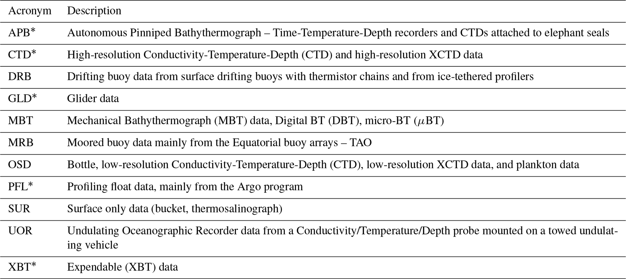
The data types marked with an asterisk (^*) are the ones used in this study.

The WOD data are structured in ragged arrays in netCDF format (https://www.ncei.noaa.gov/netcdf-ragged-array-format, last access: 29 June 2023). The structure also adheres to the CF standard conventions (https://cfconventions.org/, last access: 29 June 2023), ensuring widespread accessibility of the data. The ragged-array format is suitable for ocean profile data collections, such as WOD, where different casts can have varying counts of depth/variable pairs and different numbers of measured properties, which allows for efficient representation of oceanographic casts while minimizing file size.

In the ragged-array format, all profiles of a variable are represented by a one-dimensional array that contains all measurements. There is also a counting array called VAR_row_size, which indicates the number of measurements for each cast. To access the variable measurements for a specific cast, the VAR_row_size counts are summed, and the pointer in the array for that variable is moved accordingly. The subsequent VAR_row_size(N) elements correspond to the variable measurements for cast N.

For example, if a file contains five oceanographic CTD casts with different profiles of depth/temperature, depth/salinity, and depth/oxygen, the variables z, Temperature, and Salinity will have consistent measurements across all casts. However, the Oxygen variable may be absent in some of the casts, indicated by a zero value in the corresponding Oxygen_row_size. To read the data for a specific cast, the appropriate elements in the arrays are accessed based on the VAR_row_size counts.

We select profiles with a local depth greater than 100 m and exclude open-ocean profiles that did not reach 300 m in depth. Additionally, we exclude any data deeper than 2000 m. The WOD dataset includes flags for expeditions, instruments, and observations within each profile. We specifically consider profiles and observations with flag 0, indicating successful completion of all quality tests. Furthermore, we include profiles and observations with flag 2, which, despite passing other quality tests, shows density inversions. While density inversions are not commonly used for climatology calculations, they play a crucial role in methods such as fine-scale parameterization and Thorpe scale for estimating vertical mixing (e.g. MacDonald et al., 2013; Whalen et al., 2012).

In the pursuit of storage optimization, trade-offs often arise that can impact data usability and analysis. For example, the ragged-array format proves useful in conserving storage space by accommodating profiles of varying sizes for different properties. However, this format presents challenges when it comes to analyzing the profiles, such as performing calculations on vertical derivatives, obtaining integrated values, and comparing different properties within the same cast. To address this issue, our study develops an algorithm that facilitates the downloading, interpretation, and rearrangement of WOD data into a more user-friendly structure. The new arrangement organizes the data into two dimensions: one dimension representing the casts (casts), and a dummy dimension representing the number of levels or depths (levels). The variable z, then, depends on both levels and casts, as the vertical resolution of the measurements depends on each cast and instrument. This optimization of data structure strikes a balance between storage efficiency and enhanced usability.

The code for downloading, filtering, and restructuring the WOD dataset creates a Dask delayed object for each year. A Dask delayed object is a lazy representation of a computation. Instead of computing its result immediately, the computation is encapsulated in this object, allowing one to defer the computation until explicitly requested. This is a way to parallelize the code without an immediate evaluation; e.g. computation occurs only when compute() method is called, distributing over requested workers. In our case, we used 40 single-core Dask workers with 30 Gb of memory each.

After filtering and selecting profiles within the specified time range, we have retained a total of 4.2 million profiles. Each profile can obtain measurements for any of the selected variables: temperature, salinity, oxygen, chlorophyll, pH, and nitrate. The variables were chosen to capture both physical processes and their interactions with biogeochemical cycles, providing crucial information on the role of eddies in the regulation of climate and ecosystem health.

From 1993 to 2003, there are approximately 50 thousand profiles per year. From 2004 onward, the number of profiles per year increased to more than 150 thousand. The occurrence of each data type exhibits variability across different years and months (Fig. 1). CTD casts consistently contribute around 10 000 profiles per year throughout the entire selected time series. GLD profiles, on the other hand, were less common initially but experienced substantial growth since 2002, reaching approximately 40 thousand profiles in the last four years. In the 1990s, XBT profiles were the most prevalent, representing more than 90 % of the profiles. However, their frequency has significantly decreased, with less than 10 thousand profiles per year in the most recent four-year period. APB profiles exhibit significant variations over the years, with the majority occurring between 2004 and 2010. They were particularly abundant in 2005, surpassing 200 000 profiles, making APB the most common data type at that time. PFL profiles were relatively infrequent in the 1990s but have become the most prevalent data type since 2010, consistently surpassing 150 000 profiles from 2014 onward.

GLD, CTD, and XBT profiles do not display strong seasonality, although their occurrence is slightly reduced during holiday periods at the end and beginning of the year (Fig. 1). PFL profiles, despite appearing to exhibit some seasonality, remain relatively constant throughout the months. This apparent pattern is mainly influenced by the order of the cumulative plots. The only data type that shows a distinct seasonality is APB. Most APB profiles occur in March, April, July, and August, probably due to the seasonal behavior of the tagged animals.

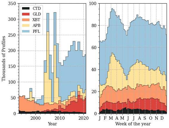
Figure 1 Cumulative distribution of WOD profiles by data type varying with years (a) and months (b). Each bar in (b) represents a week, and the major ticks mark the first week of each month.

The global distribution of profiles exhibits distinct characteristics for each data type. PFL profiles demonstrate a significantly more homogeneous distribution, with the exception of the region close to Antarctica (Fig. 2a). In contrast, XBT profiles reveal well-defined routes corresponding to commercial ships, predominantly observed in the North Atlantic (Fig. 2b). The distribution of GLD data is notably concentrated in specific regions with a high density of profiles (Fig. 2c). The CTD casts mainly concentrate in the Kuroshio and Gulf Stream regions, with additional profiles observed in the equatorial region (Fig. 2d). APB profiles, on the other hand, are prominently concentrated in the Northeast Pacific and in the Antarctic Circumpolar region south of the Indian Ocean (Fig. 2e).

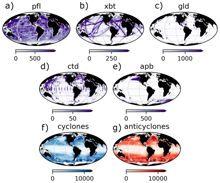
Figure 2 Global distribution of WOD profiles for PFL (a), XBT (b), GLD (c), CTD (d), APB (e), META3.2 DT cyclonic eddy observations (f) and anticyclonic eddy observations (g). The data shown here is after quality-control steps and application of filters described in the text.

Mesoscale eddy atlas

The central component of this study is the characterization of the mesoscale eddies identified in the sea-level data. For this purpose, we employ the Mesoscale Eddy Trajectory Atlas META3.2 DT, a new eddy tracking census that replaces previous products distributed by AVISO¹ or CMEMS². Specifically, we use the delayed-time all-satellite atlas (META3.2 DT all-satellites, https://doi.org/10.24400/527896/a01-2022.005.210802, Pegliasco et al., 2022b), which identifies a total of 36 522 562 cyclonic eddy observations and 34 521 490 anticyclonic eddy observations in the CMEMS product described above. Here, we refer to the META3.2 DT product as Eddy Atlas.

Pegliasco et al. (2022a) describes a beta version of META3.2 DT Eddy Atlas, the META3.1exp product, and compares it with META2.0 and other atlases (Chelton et al., 2011; Mason et al., 2014). Eddies are identified as closed sea-surface height contours around local extrema, and tracked through time based on spatial overlap and similarity of their geometric properties across consecutive days, as described in Pegliasco et al. (2022a). This results in persistent eddy identifiers that enable the reconstruction of full eddy lifetimes. Only a few minor changes were made from the experimental version 3.1 to the current version 3.2 DT, and the description of 3.1exp in Pegliasco et al. (2022a) is generally valid for 3.2. A main novelty in META3.2 DT compared to META 2.0 is the identification of Eulerian mesoscale eddies as closed contours of spatially high-pass filtered sea-surface height in lieu of closed contours of filtered sea-level anomaly. The use of sea-surface height allows for better detection of eddies near strong currents and steep topography, and is key to a good representation of eddies that grow locally on top of standing meanders. META3.2 DT also changed the eddy detection from Chelton et al.'s eddy-tracking lineage of algorithms to an upgraded version of the algorithm by Mason et al. (2014). META3.2 DT further implemented a few minor changes to error thresholds, filtering of large-scale signals (reducing the half-power scale from 1000 km to 700 km), a reduced sea-level interval to search for the eddy edges, etc. Globally, META3.2 DT has an increased number of eddies compared to META2.0, but most of these extra eddies are small, short-lived eddies and will not be considered in our analysis.

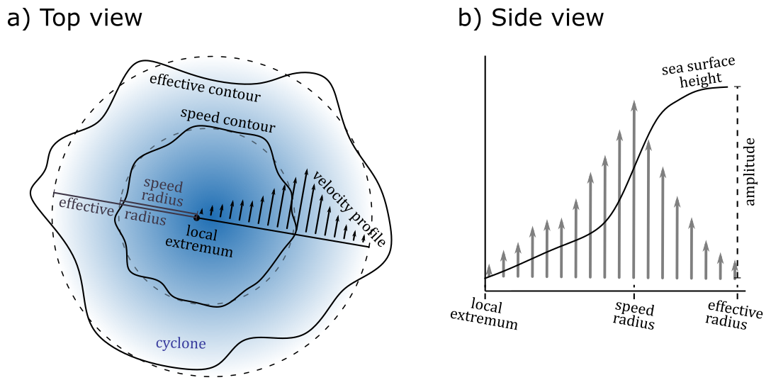
Figure 3 Illustrative example of the eddy characteristics associated with a cyclone in the northern hemisphere. (a) Top view: Solid lines indicate two sea-surface height contours (effective and speed contours) encompassing the local extremum, which represents the eddy center. Dashed lines represent circle approximations of each contour, determining the radii. Arrows depict the tangential velocity profile within the eddy. (b) Side view: The solid line represents the sea-surface height, with the amplitude calculated as the sea-surface height difference between the effective contour and the eddy center.

In addition to basic eddy characteristics (e.g., trajectories, amplitude, swirl speed, and size), META3.2 DT provides details for each eddy observation, including the coordinates for sea-level contours (Pegliasco et al., 2022a). (A difference between 3.1exp and 3.2 DT is that 20-point contours instead of 50-point contours are now provided.) These added details on the eddy shape allow us to match the WOD profiles with META3.2 DT. For reference, it is helpful to define a few eddy properties that are already included in META3.2 DT (see Fig. 3 as reference):

• Effective contour: outermost high-pass filtered closed contour of sea-surface height detected from a search starting at the localized sea-level extremum.

• Speed contour: high-pass filtered closed contour of sea-surface height associated with maximum azimuthally averaged velocity detected from a search starting the localized sea-level extremum.

• Effective radius: eddy radius obtained by fitting a circle to the effective contour.

• Speed radius: eddy radius obtained by fitting a circle to the speed contour.

• Eddy center: coordinates (longitude, latitude) of the high-pass filtered extremum of sea-surface height obtained from fitting a circle to the speed contour.

• Amplitude: difference in sea-surface height between the effective contour and the local extremum.

• Effective velocity profile: profile of azimuthally averaged velocity from eddy center to effective radius.

• Speed velocity profile: profile of azimuthally averaged velocity from eddy center to speed radius.

• Average speed: azimuthally averaged speed associated with the speed radius.

We also add other eddy properties, such as the Rossby number $\left(Ro={\displaystyle \frac{U}{Lf}}\right)$: defined by the maximum azimuthal velocity (U), local planetary vorticity (f) and speed radius (L).

We employ a series of filtering criteria to extract significant eddy observations from the datasets based on Rocha and Simoes-Sousa (2022). Firstly, we discard eddies whose time-mean amplitudes are smaller than 2.5 cm and whose first detection is centered at depths shallower than 200 m to avoid variability related to sampling noise and defective tidal corrections on the shelf. Next, we remove eddies with a duration of less than 30 d, focusing on long-lived eddies that potentially play a more substantial role in ocean dynamics. To facilitate subsequent analysis and data subset selection, we save the observations of the filtered eddies in separate NetCDF files. Each file corresponds to a specific year and month, enabling a more efficient and organized approach for further investigation using parallel processes. To accelerate the filtering process, we partition the data into approximately 120 chunks, each containing around 300 000 vortex observations. These chunks are processed using 60 single-core Dask workers, each allocated 5 GB of memory.

We retain a total of 18 785 117 cyclonic eddy observations and 17 933 921 anticyclonic eddy observations used to combine with the profiles. This leads to a total of 205 770 and 190 031 unique cyclones and anticyclones, respectively. For clarity, throughout the manuscript, we refer to eddy observations as individual daily detections of eddies (i.e., one snapshot per eddy per day), while unique eddies denote the complete trajectories of those eddies over time, encompassing all daily observations from formation to dissipation. Each unique eddy is assigned a persistent identifier in the META3.2 DT atlas, enabling the temporal association of multiple profiles with the same eddy over its full lifetime.

Observations of anticyclones are slightly less common than those of cyclones, with an average of 616 309 observations per year compared to 645 569 observations of cyclones per year. On a global scale, there is no significant difference in the occurrence between cyclones and anticyclones (Fig. 2f–g). However, we observe distinct patterns at local scales. Anticyclones tend to be more frequent offshore in proximity to western-boundary currents, while cyclones are more common inshore to these currents. Both cyclones and anticyclones are more frequent in regions characterized by strong meandering currents, such as the Northwest Atlantic and Brazil-Malvinas.

During our filtering process, we exclude low-amplitude eddies, resulting in a decrease in eddy occurrence within an equatorial latitudinal band of ±10°. The Northeast Pacific has traditionally been considered an “eddy desert” with low eddy occurrence (Whalen et al., 2018). However, recent studies have revealed that this region is, in fact, rich in Lagrangian eddies (Liu and Abernathey, 2023). It is noteworthy that this particular region exhibits a high concentration of APB profiles in our dataset. In future releases, there is potential to expand our analysis by combining the WOD dataset with the Lagrangian eddy atlas, enabling a more comprehensive exploration of this region.

Combining datasets

This study introduces a novel contribution in the form of the global vortex-profile matching dataset. Currently, we employ the eddy effective (most external) contour to delineate the boundaries of the eddies. Users can restrict the analysis to the speed core of the eddy by filtering out profiles within a radius of speed.

For each matched profile–eddy pair, we include the full set of eddy properties at the time of observation – such as eddy center coordinates, effective and speed radii, amplitude, average velocity, and Rossby number – along with the unique eddy identifier. Because this identifier persists throughout the eddy’s lifetime, it allows users to reconstruct the full eddy trajectory and time series of properties. The dataset also retains the profile's original location, depth, timestamp, and instrument metadata, enabling composite analyses of the vertical and temporal structure of long-lived eddies.

The matching algorithm we developed enables parallelization for each year, encompassing both profile data and eddy observations. For each profile data type, e.g. CTD, we iterate through each cast and examine whether it resides within the effective contour of any eddy located in a 10×10° square centered around the profile. The 10×10° search area reduces computational time by matching only vortices close to the profile. Our decision to iterate over the profiles rather than the eddy observations stems from the fact that, by definition, an eddy observation can comprise multiple profiles, whereas a profile can only be associated with a single eddy. If the profile falls within an eddy, we append all eddy parameters to the cast.

The parallelization is done by using a Dask delayed function applied for each year and month, generating a list of delayed objects that are further parallelized to multiple cluster workers. In our case, we use 100 single-core workers with 5 Gb of memory each, totaling 500 Gb of simultaneous memory allocated.

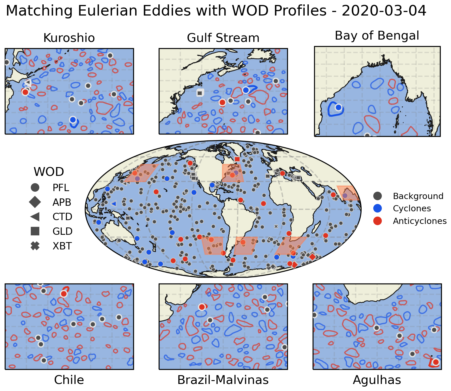
Figure 4 Global distribution of WOD profiles on 4 March 2020. Each data type is represented by a specific marker: circle (PFL), diamond (APB), triangle (CTD), square (GLD), and X (XBT). Profiles within anticyclones are marked in red, profiles within cyclones in blue, and background profiles in gray. Zoomed panels highlight six regions: Kuroshio, Gulf Stream, Bay of Bengal, Chilean coast, Brazil-Malvinas, and Agulhas. The panels display profiles and eddy speed contours, with thicker lines indicating eddies containing at least one profile. An animated version is available at https://www.youtube.com/watch?v=9xzhtrzLRdo (Simoes-Sousa, 2025).

Our comparison of the WOA climatology with our own climatology based on the background profiles reveals no discernible differences (not shown). One plausible hypothesis is that, while numerous, the eddies do not cover a large relative area of the ocean's surface. For example, in 2015, the average area covered by the long-lived eddies was only 13 ± 0.2 % of the total ocean surface from 60° S–60° N, which ballparks the 12.6 % of the total drifting profiles (PFL) located within the eddies. This is further corroborated by the low percentage of PFL profiles found in unique vortices (Fig. 5). Although only 5 % of the unique vortices contain more than 10 PFL profiles, there is still a significant number of trapping events, with 2462 unique anticyclones and 2295 unique cyclones each having at least 10 profiles during their lifetime. These events lend themselves to specific case studies that follow individual eddies.

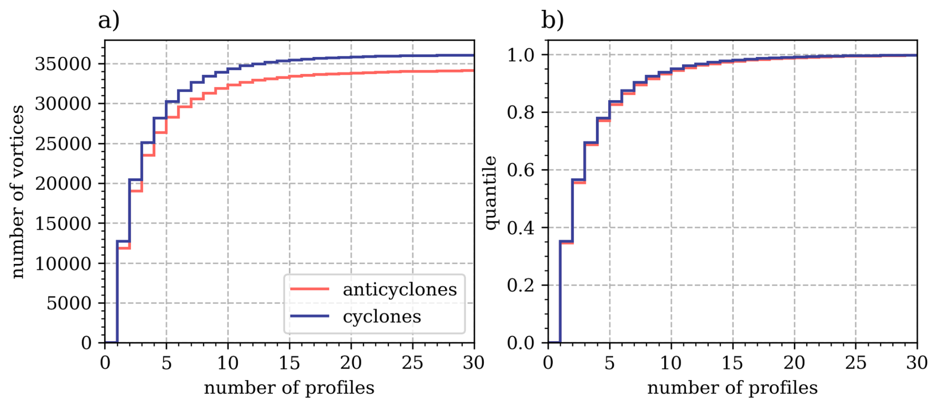
Figure 5 Cumulative distribution for the absolute (a) and relative (b) total number of PFL profiles over the full lifetime of unique anticyclones (red) and cyclones (blue).

To provide a comprehensive representation, we present the vortex-profile matching on a global scale (center panel, Fig. 4). Although certain geographic regions display a high occurrence of eddies, most of the profiles lie outside them, even in highly energetic areas such as the Kuroshio, Gulf Stream, Brazil-Malvinas, and Agulhas (as shown in the zoomed-in panels in Fig. 4).

Following the successful matching of each profile to its respective eddy, we consolidate all profiles and store the combined dataset based on the variable and the inclusion of profiles within eddies. In other words, for each dataset and variable, we generate two distinct files: one containing profiles within eddies, and another file for background profiles.

Following the recommendations of TEOS-10 (IOC, SCOR and IAPSO, 2010), the dataset stores only measurements on-site, avoiding storing derived variables. However, we added an example of how to compute the conservative temperature and absolute salinity anomalies referenced to the climatology in the code repository.

4 Dataset availability

The dataset is available through the Open Source Project for a Network Data Access Protocol (OPeNDAP) server at the University of Massachusetts Dartmouth (UMassD) and at Woods Hole Oceanographic Institution (WHOI). We also provide a faster option for users to access the data through an Amazon Web Services (AWS) S3 bucket in icechunk format. Users have the flexibility to subset the dataset based on their desired time range and region by directly accessing it with software such as Python XArray.

Using an OPeNDAP server and an S3 bucket to store the dataset offers several advantages. First, it provides a convenient and efficient means of data access, enabling users to retrieve subsets instead of having to download the entire dataset and subset it locally. This reduces the need for large data transfers and storage requirements on the user's end. Additionally, these options support remote data access, allowing researchers to access and analyze the dataset from different locations, promoting collaboration, and facilitating data sharing within the scientific community. Moreover, an OPeNDAP server enables future on-the-fly data processing, such as subsetting, aggregation, and interpolation, which can be advantageous for large and complex datasets, as it reduces the need for pre-processing and minimizes storage demands. Additionally, we also provide the vortex-profile dataset to download from an HTTP server.

5 Data Validation

One of the preliminary results of this dataset is the global distribution of temperature, salinity, and density anomalies. In this analysis, the combined dataset is partitioned into manageable chunks, each comprising approximately 800 casts. To handle the computational demands efficiently, we parallelize the analysis, employing 50 single-core workers, each provisioned with 3 Gb of memory. We take advantage of the capabilities of the XHistogram (https://xhistogram.readthedocs.io/en/latest/index.html, last access: 8 December 2025) package to compute the distribution of anomalies. This package seamlessly integrates with both XArray and Dask for computing multi-dimensional histograms. For enhanced granularity in our estimations, the distributions are calculated at intervals of every 25 m in depth and spatially over 5×5° grid boxes.

Generally, anticyclones appear to be more intense than cyclones in thermal and saline anomalies, and the patterns in the vertically-averaged anomalous properties highlight the strongly energetic boundary-current regions. As anticipated, cyclones, being low-pressure systems, generate upward displacement of the isopycnals and are strongly associated with negative temperature anomalies (Fig. 6a). Conversely, anticyclones, as high-pressure systems, are linked to positive temperature anomalies (Fig. 6b). The patterns in global eddy salinity anomalies are less apparent and likely depend on the distribution of water masses across the globe and the rotational sense of the eddies, sometimes compensating temperature anomalies, and, sometimes strengthening them. For most oceans, cyclones are accompanied by compensating negative salinity anomalies, with the exception of the Mediterranean Sea (Fig. 6c). Salinity anomalies in anticyclones exhibit regional variations, with western boundary currents displaying positive anomalies and other regions exhibiting both positive and negative anomalies (Fig. 6d). Cyclones show weaker negative temperature anomalies and more negative salinity anomalies compared to anticyclones, resulting in a weaker signal in the potential density anomalies (Fig. 6e, f), with some unexpected positive anomalies observed in a few regions.

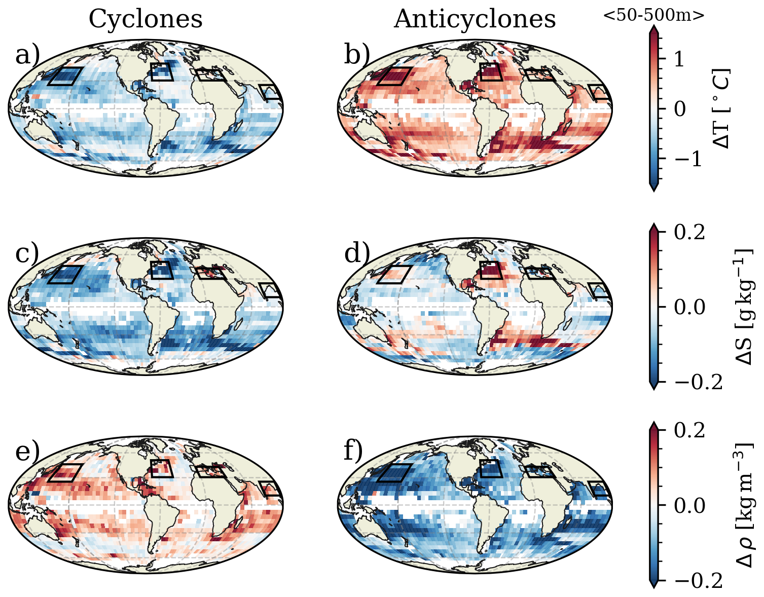
Figure 6 Global distributions of anomalies in conservative temperature (°C, panels (a) and (b)), absolute salinity (g kg⁻¹, (g), (c) and (d)), and potential density (kg m⁻³, (e) and (f)) within cyclones (a, c, e) and anticyclones (b, d, f). The anomalies correspond to median profiles computed within 5×5° boxes subsequently averaged between depths of 50 and 500 m. The black solid lines indicate the regions where the vertical distribution of properties was analyzed. Boxes with less than 10 profiles are masked.

The expected positive temperature anomalies for anticyclones and negative temperature anomalies for cyclones serve as a reliable quality control measure for the vortex profile matching method. Despite the intriguing unexpected patterns observed in the anomalous salinity of the eddy, the stratification of the ocean is mostly dominated by temperature changes, and the consistency of temperature anomalies within the eddies confirms the accuracy and robustness of the method.

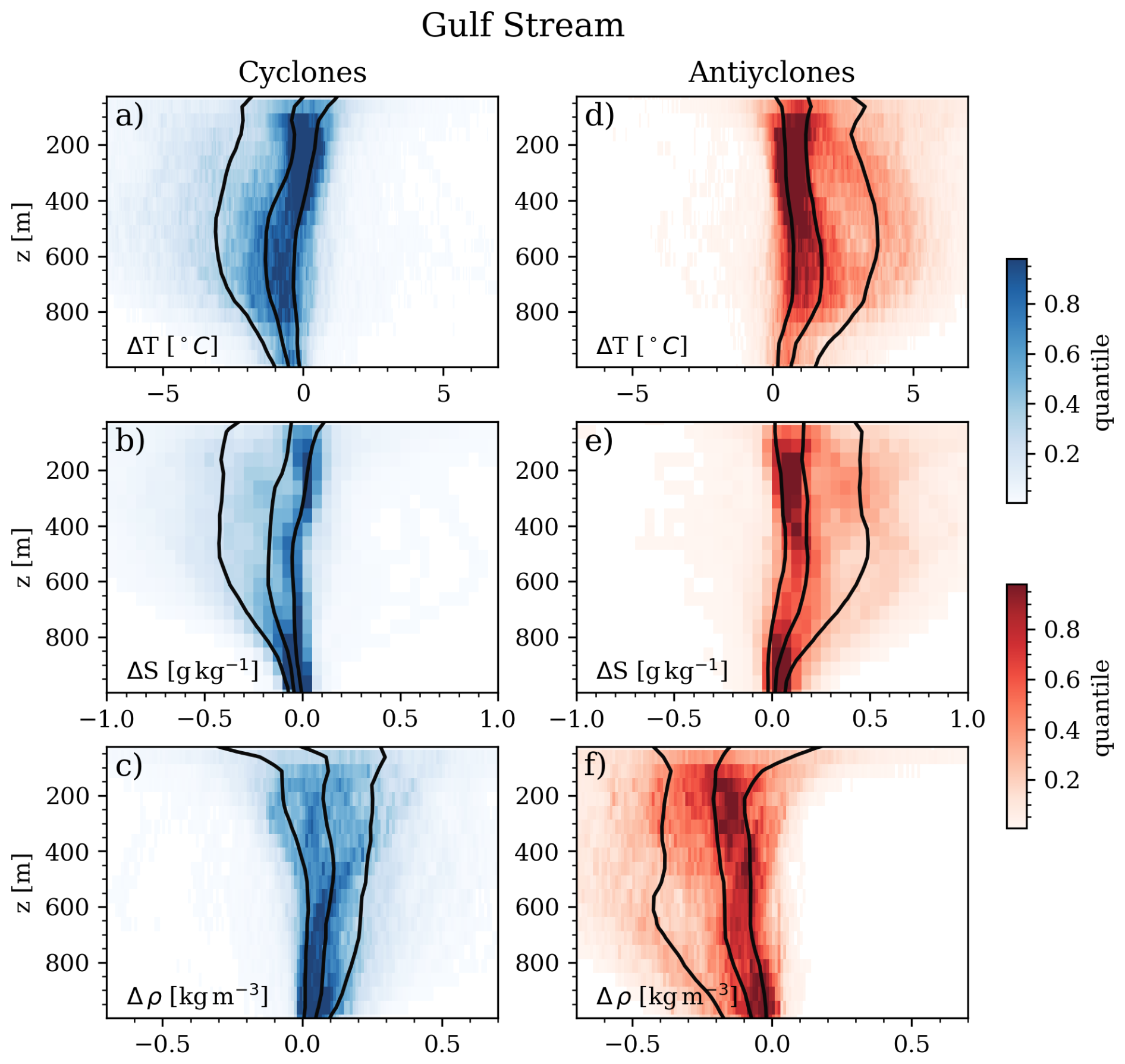
Figure 7 Median anomalous vertical profile conservative temperature (°C, panels (a) and (d)), absolute salinity (g kg⁻¹, (b) and (e)), and potential density (kg m⁻³, (d) and (f)) within cyclones (a, b, c) and anticyclones (d, e, f) for the Gulf Stream region. Black solid lines represent the 20th, 50th and 80th percentiles.

Next, we expand our perspective and analyze the vertical distribution of anomalies for the first 1000 m in different regions. The regions are chosen based on the intensity of vortical activity (Gulf Stream and Kuroshio Current) or due to their exceptional patterns of temperature and salinity (Bay of Bengal and Mediterranean Sea). The anomalies in the Gulf Stream extend to the whole 1000 m range for both cyclones and anticyclones. The general median temperature anomalies reach 1.5 °C around 600 m with the 80th percentile around 4 °C for both cyclones (negative) and anticyclones (positive), although the distribution for anticyclones is bimodal, showing a branch peaking at 5 °C around 500 m (Fig. 7a, d). The salinity anomalies corroborate the patterns shown in Fig. 6, with negative values within cyclones and positive within anticyclones (Fig. 7b, e). The median peaks around 0.2 g kg⁻¹ at 600 m with the 80th percentile reaching 0.5 g kg⁻¹. The density anomalies follow the expected patterns of the combined effect of temperature and salinity (Fig. 7c, f). The vertical structure and anomalies associated with anticyclones (warm core rings) are corroborated by a recent study that employed a totally independent method (see Fig. 7 from Silver et al., 2022). The description and analysis of mesoscale eddies in the Gulf Stream encompass a wide variety of applications, including the behavior of the top predators. For example, Gaube et al. (2018) reveals the extensive use of anticyclones (warm-core rings) by mature white sharks, suggesting that anomalies make prey more accessible and energetically profitable.

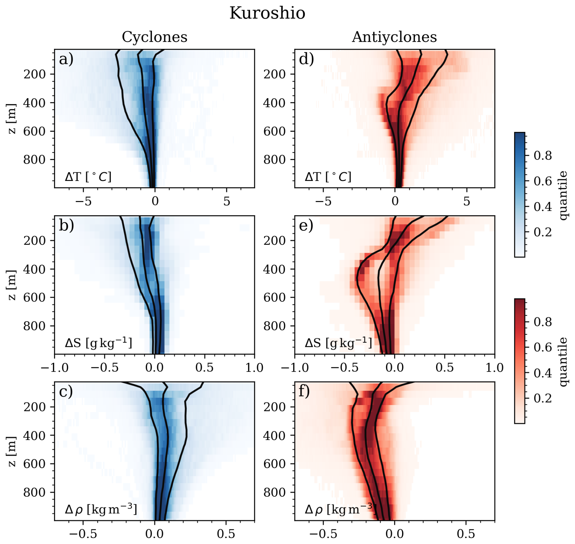
Figure 8 Median anomalous vertical profile conservative temperature (°C, panels (a) and (d)), absolute salinity (g kg⁻¹, (b) and (e)), and potential density (kg m⁻³, (d) and (f)) within cyclones (a, b, c) and anticyclones (d, e, f) for the Kuroshio Current region. Black solid lines represent the 20th, 50th and 80th percentiles.

Turning our attention to Kuroshio, we find negative temperature anomalies for cyclones, with a median value of approximately −1 °C (80th percentile around −3 °C), extending to depths of around 800 m (Fig. 8a). In contrast, anticyclones exhibit predominantly positive temperature anomalies, with a median value of around 2 °C (80th percentile around 3.5 °C), more concentrated near the surface and shallower in depth compared to cyclones (approximately 500 m) (Fig. 8d). The salinity anomalies of the cyclones show negative values that intensify near the surface, with a median of approximately −0.15 g kg⁻¹ (80th percentile of around −0.4 g kg⁻¹), extending to depths of 700 m (Fig. 8b). Within anticyclones, the salinity anomaly patterns exhibit a bimodal distribution, with a branch that transitions from positive values on the surface to a negative peak around 500 m (Fig. 8e). The median anticyclonic salinity anomalies range from negative to positive values around 0.2 g kg⁻¹, with the 80th percentile approximately 0.4 g kg⁻¹. The peak values and the vertical structure corroborate the findings reported in a recent study conducted in the region (Sun et al., 2017), although notable salinity inversions are not observed in our analysis for cyclones. Within cyclones, the density anomalies exhibit a slightly positive median (less than 0.1 kg m⁻³), with the 20th percentile showing negative anomalies at the surface around −0.2 kg m⁻³ (extending to 300 m). The 80th percentile demonstrates positive anomalies, extending to 1000 m with a typical value of 0.3 kg m⁻³. In contrast, anticyclones display a negative median density anomaly (around −0.2 kg m⁻³), peaking at approximately 400 m depth. The 80th percentile also reveals negative anomalies, extending to 1000 m with a typical value of −0.3 kg m⁻³.

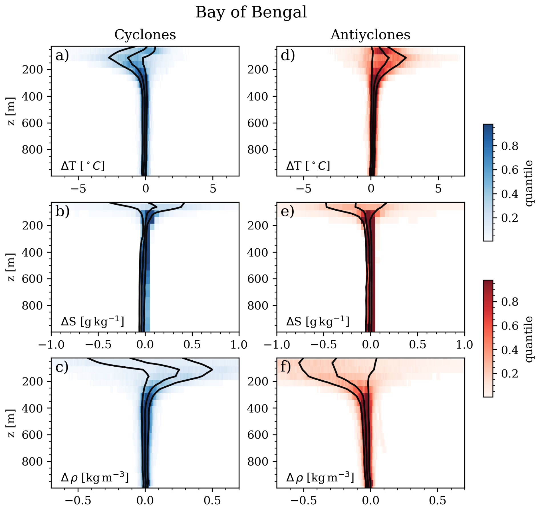
Figure 9 Median anomalous vertical profile conservative temperature (°C, panels (a) and (d)), absolute salinity (g kg⁻¹, (b) and (e)), and potential density (kg m⁻³, (d) and (f)) within cyclones (a, b, c) and anticyclones (d, e, f) for the Bay of Bengal region. Black solid lines represent the 20th, 50th and 80th percentiles.

The vortices in the Bay of Bengal are shallower than in other regions (approximately 300 m) and exhibit a temperature and density peak around 100 m depth (Fig. 9). The signals and vertical structure of the temperature and density anomalies support a recent study that used regional vortex-profile matching Lin et al. (2019). However, the absolute salinity values presented by Lin et al. (2019) are more intense and less spread, likely due to their consideration of the profile position relative to the vortex center, which is not taken into account in our analyses. The greater variability of salinity anomalies near the surface is also characteristic of the region, which features multiple river plume fronts and monsoonal rainfall that can generate surface freshwater lenses (Gordon et al., 2016; Jensen et al., 2016; Shroyer et al., 2021). Understanding the dynamics of mesoscale vortices is crucial for predicting salinity transport pathways in the Bay of Bengal and its exchanges with the Equatorial Indian Ocean and Arabian Sea (Jensen et al., 2016; Hormann et al., 2019).

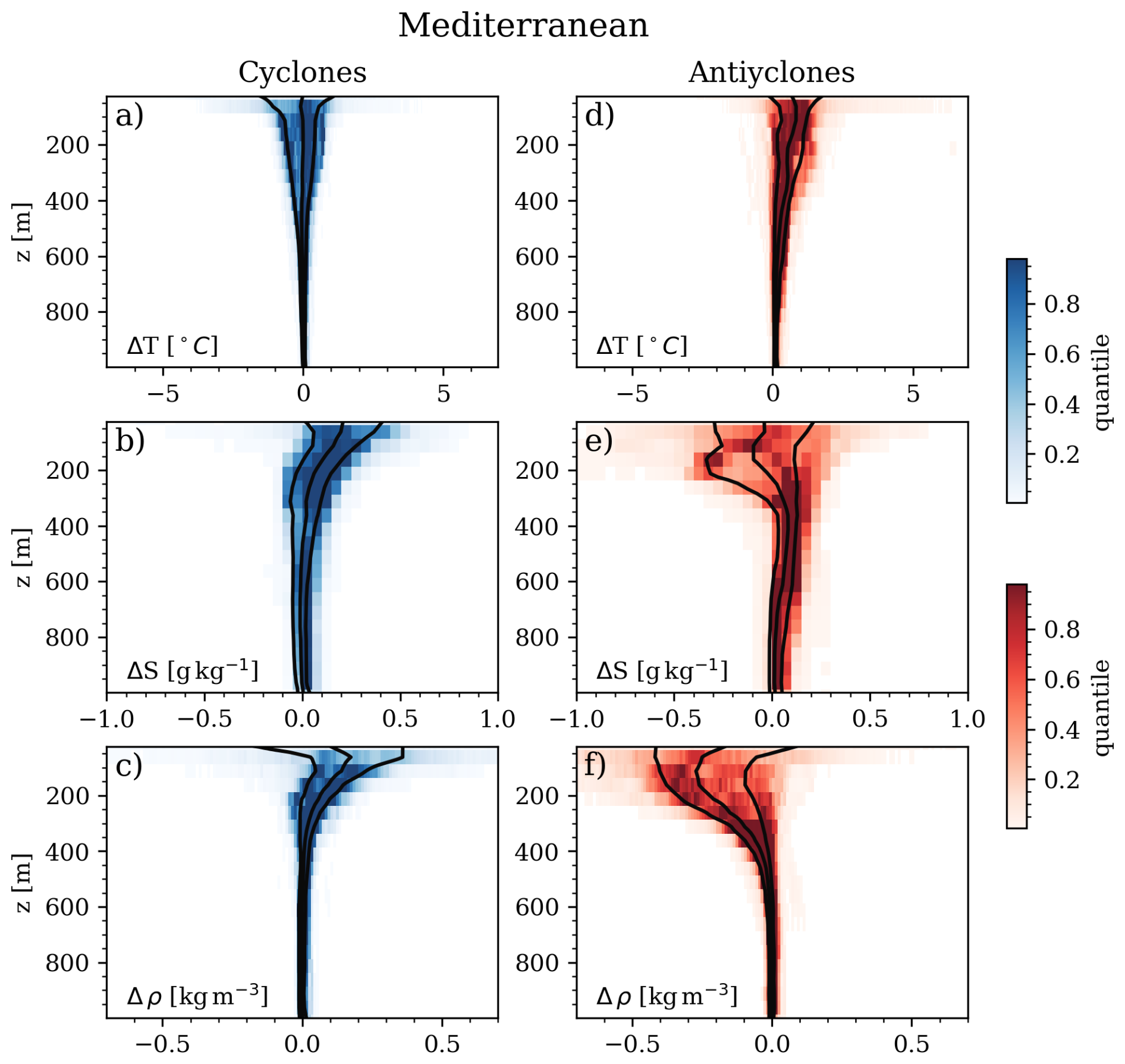
Figure 10 Median anomalous vertical profile conservative temperature (°C, panels (a) and (d)), absolute salinity (g kg⁻¹, (b) and (e)), and potential density (kg m⁻³, (d) and (f)) within cyclones (a, b, c) and anticyclones (d, e, f) for the Mediterranean Sea region. Black solid lines represent the 20th, 50th and 80th percentiles.

Mesoscale eddies play a significant role in shaping the dynamics of the Mediterranean Sea, contributing substantially to sea-surface height variability and kinetic energy at various depths (50 %–60 %, Bonaduce et al., 2021). In this region, the temperature structure of cyclones exhibits a broad distribution, with a median around zero, indicating the presence of both warm-core and cold-core cyclones (Fig. 10a). While temperature does not seem to heavily influence density anomalies in the region, anticyclonic anomalies show a slightly positive curve, extending to a depth of 400 m with temperature values below 1 °C (Fig. 10). On the other hand, salinity anomalies have a greater impact in the Mediterranean Sea compared to temperature anomalies. Cyclonic salinity anomalies display an exponential-like decay, with a median of 0.2 g kg⁻¹ at the surface, declining to zero at 300 m (Fig. 10b). The 80th percentile reaches 0.4 g kg⁻¹ at the surface. For anticyclones, salinity anomalies remain relatively constant at −0.1 g kg⁻¹ for the first 200 m (with the 80th percentile around −0.3 g kg⁻¹) before decreasing to zero at 300 m (Fig. 10e). Despite anticyclones exhibiting shallower salinity anomalies compared to cyclones, the combined effect of slightly positive temperature anomalies and negative salinity anomalies leads to stronger and deeper density anomalies (Fig. 10c, f). The vertical structure of mesoscale eddies in the Mediterranean Sea varies regionally and seasonally, yet the overall patterns described here align with recent findings, which illustrate that anticyclones extend to greater depths (up to 400 m) than cyclones (first 200 m) in the region (see Fig. 10 from Bonaduce et al., 2021).

6 Future directions and potential applications

The analyses in Sect. 5 serve a dual purpose: firstly, to perform a quality check on the dataset by comparing the results with published literature, and secondly, to demonstrate the potential of the dataset for conducting global analyses of the vertical structure of mesoscale eddies. It is important to acknowledge that the current version of the analyses presented in this study focuses primarily on temperature, salinity, and density anomalies, not taking into account other biogeochemical variables, the radial distance of the profiles from the eddy center, as well as seasonal and interannual variability. However, it is worth noting that these additional properties are available within the dataset and hold great potential for future investigations. By incorporating these variables into our analyzes, we can gain a more comprehensive understanding of the complex dynamics and drivers underlying the behavior of mesoscale eddies.

7 Code and data availability

The dataset used in this study is publicly available at https://doi.org/10.5281/zenodo.17425853 (Simoes-Sousa et al., 2025).

Updated links and the status of the servers, including access through Amazon Web Services S3 bucket, are listed in the GitHub repository. The code for processing and analyzing the dataset, including the vortex-profile matching algorithm, is available on Zenodo (Simoes-Sousa, 2025, https://doi.org/10.5281/zenodo.14681279) and GitHub (https://github.com/iuryt/vortex_profile_matching, last access: 8 December 2025). Users can access the data and code for reproducibility and further research.

8 Conclusions

In this study, we construct a unique dataset by combining temperature, salinity and biogeochemical profiles from the World Ocean Database (WOD) with Eulerian mesoscale eddies identified and tracked using altimetry data (META3.2 DT). We have demonstrated the potential dataset's utility to explore global characteristics of mesoscale eddies, including their vertical extension and salinity compensation to temperature anomalies.

The primary objective of this work is to develop a comprehensive global dataset for studying the vertical structure of mesoscale eddies identified through altimetry data. We are committed to the principles of open, transparent, and accessible science, with a strong focus on reproducibility. To facilitate spatial, temporal, and source-based subset analyses, we have organized the data in a manner that supports on-the-fly remote data analysis through an OPeNDAP server, AWS S3 bucket, as well as through direct download by HTTP.

This dataset represents a powerful tool for advancing our understanding of ocean processes, enabling detailed studies on mesoscale eddy dynamics, their role in biogeochemical cycles, and their influence on regional and global ocean circulation. By integrating in situ measurements with satellite-derived eddy tracking, this resource provides a foundation for addressing fundamental questions in oceanography and offers broad potential for applications in climate science, ecosystem modeling, and operational oceanography.