Sea level reconstruction reveals improved separation of regional climate and trend patterns over the last seven decades

Rapidly rising sea level is one of the major adverse consequences of anthropogenic climate change. Sea level rise poses an existential threat to coastal populations, particularly for urban settlements with accelerating growth rates. Contemporary empirical sea level reconstructions have been used to conflate short-term (∼ 3 decades) satellite altimetry geocentric sea level data and long-term (50 years or longer) tide gauge records to better estimate reliable sea level rise towards multi-decadal to centennial time scales. However, adequate separations and quantifications of low-frequency climate patterns and sea level trends globally at regional scales remain elusive. Here, we propose a new sea level reconstruction framework that incorporates Empirical Orthogonal Function (EOF) into the contemporary Cyclostationary EOF with Reduced Space Optimal Interpolation (CSEOF-OI) algorithm to better reconstruct sea level fields. Using 225 selected long-term gap-filled tide gauge records with vertical land motion adjusted and satellite altimetry, our global reconstructed monthly sea level time series, January 1950–January 2022, exhibits distinct delineations between modeled climate patterns and sea level trends at 1°×1° regional scales. The separated sea level patterns include trends, modulated annual cycles, the El Niño Southern Oscillation (ENSO), and the Pacific Decadal Oscillation (PDO). The third principal component of the reconstructed sea level exhibits a Pearson correlation coefficient of 0.87 with the Niño 3.4 ENSO index, and the fourth principal component correlates at 0.75 with the PDO index, indicating good agreement. The global mean sea level trend, accounting for the predominant climate periodicities, is 1.9 ± 0.2 mm yr⁻¹ (95 % confidence), and the estimate during the satellite altimetry era (January 1993–December 2021) is 3.2 ± 0.3 mm yr⁻¹ (95 % confidence). Compared with previous studies, we conclude that our 72-year sea-level reconstruction allows us to better separate the ENSO and PDO climate patterns, as well as the sea level they induced. Finally, we show that the short-term (5-year) rates of ENSO and PDO patterns significantly affect sea level both on a global and regional scale, altering global mean sea level trends by up to 1.1 ± 0.5 mm yr⁻¹ (January 2011–January 2016). Over the past seven decades, the climate patterns exerted a minor impact on sea level trends, but substantially modulated apparent regional sea level accelerations, particularly in the western Pacific (e.g., 0.09 ± 0.05 mm yr⁻² at the Kuroshio Current), and in the east and central equatorial Pacific Ocean (e.g., −0.04 ± 0.03 mm yr⁻² near Costa Rica). The reconstructed sea level and analysis results datasets are available at https://doi.org/10.5281/zenodo.15288816 (Wang, 2025).

1 Introduction

Sea level rise poses a significant and existential threat to humanity's well-being now and for the foreseeable future. Recent studies reveal that global mean sea level rise has increased from 2.1 mm yr⁻¹ in the early 1990s to 4.5 mm yr⁻¹ by 2023 (Hamlington et al., 2024). Sea level projections show that by 2100, even under a low carbon emission scenario, sea level will continue to rise (National Research Council, 2012), and it is estimated that 150 to 250 million people will live in areas at risk of tidal submersion due to rapid sea level rise (Kulp and Strauss, 2019). Anthropogenic greenhouse warming probably preceded the Industrial Revolution, mostly in response to agriculture and changes in land use, but accelerated once the Industrial Revolution drove accelerating emissions of greenhouse gases into the atmosphere. Warming of the oceans and mass transfer from the cryosphere to the oceans have dominated the rise in sea level for more than one century (Walker et al., 2022). Present-day sea level change is influenced by a range of geophysical processes, including oceanic thermal expansion (Feng and Zhong, 2015), ablation of Earth's ice reservoirs, anthropogenic water impoundment in reservoirs and dams, water transfers between oceans, ice reservoirs, and continents (Shum and Kuo, 2010), seafloor deformation driven by deep-earth processes such as glacial isostatic adjustment (Tamisiea, 2011), geocenter motion, and to a lesser extent, changes in seawater salinity (Wang et al., 2022). According to the World Climate Research Programme (WCRP) global sea level budget group, 42 % of the mean sea level rise from 1993 to 2015 can be attributed primarily to thermal expansion of the oceans, with contributions from mountain and peripheral glaciers, and the ice sheets of Greenland and Antarctica accounting for 21 %, 15 %, and 8 %, respectively (WCRP Global Sea level Budget Group, 2018). After accounting for the gravitational tidal variations from the Sun and the Moon, the origins of Earth's present-day long-term sea level include annual or longer (up to multi-decadal, and perhaps to centennial) oceanic oscillations from interactions between the ocean, atmosphere, hydrology, cryosphere, solid Earth, and anthropogenic contributions including human impoundment/pumping of water in reservoirs/groundwater. These changes range from interannual to multi-decadal timescales and potentially extend to the century timescale, or even longer.

The advent of satellite radar altimetry since the early 1990s has revolutionized the monitoring of global sea level. However, satellite altimetry measurement records are too short to determine the rate of rapid or accelerated sea level rise (Iz et al., 2018; Iz and Shum, 2021), especially considering the inability to characterize sea level acceleration at regional scales, from sparsely located long-term tide gauge records and due to the presence of multi-decadal or longer (low frequency) oceanic signals (Chambers et al., 2012; Iz and Shum, 2021).

The empirical reconstruction has been widely employed to study multi-decadal spatiotemporal changes in sea level. The contemporary methodology integrates temporally extensive but spatially limited records from tide gauges – whose vertical land motion is accounted via glacial isostatic adjustment (GIA) models, Global Navigation Satellite System (GNSS) observations, or the satellite altimetry minus tide-gauge difference (see Sect. 2.2) – and satellite altimetry measurements that provide extensive spatial coverage and resolution, but with limited temporal duration. By applying methods such as Reduced Space Optimal Interpolation (RSOI) to synthesize data, this approach enables comprehensive empirical modeling of sea level changes and dynamics spatiotemporally, extending from the altimetry era back to pre-altimetry periods (Church et al., 2004; Church and White, 2006; Berge-Nguyen et al., 2008; Church and White, 2011; Ray and Douglas, 2011; Meyssignac et al., 2012). Recent innovations have further refined the accuracy of historical sea level reconstruction, introducing the Cyclostationary Empirical Orthogonal Function with Reduced Space Optimal Interpolation (CSEOF-OI) to capture sea level variability better and reduce sensitivity to the spatial distribution of tide gauges, when compared to previous RSOI-based approaches (Hamlington et al., 2011, 2014; Strassburg et al., 2014).

Apart from RSOI-based approaches, the Kalman Smoother (KS) method integrates climate fingerprints – such as ice melt and glacial isostatic adjustment (GIA) – along with steric dynamic priors from ocean models, fitting the information to tide gauge records to reconstruct sea level (Hay et al., 2013, 2015; Frederikse et al., 2018, 2020). The KS method has proven more effective in capturing long-term sea level trends, whereas RSOI excels in reconstructing sea level variability. This has led to the development of hybrid reconstructions (HR) that utilize KS for estimating trends and RSOI for sea level variability (Dangendorf et al., 2019, 2024).

Despite these methodological advances, the fidelity of reconstructed sea levels – especially in distinguishing the impacts of various climate patterns – remains a significant challenge. The Modulated Annual Cycle (MAC) and the El Niño-Southern Oscillation (ENSO) are known to be two major drivers of climate pattern-induced sea level changes, and their influences are quantified globally at a regional scale by analyzing multi-decadal reconstructed sea level (Hamlington et al., 2011; Hamlington et al., 2014; Mu et al., 2018; Wang et al., 2024).

The Pacific Decadal Oscillation (PDO) is another climate pattern exerting a significant influence on North Pacific Sea surface temperature anomalies (SSTa), with its broader implications for global sea level changes increasingly noted in recent studies (Si and Xu, 2014; Han et al., 2017). However, the task of disentangling the sea level changes induced by ENSO and PDO is challenging due to their similarity and strong correlation.

To address the challenges and more accurately delineate sea level trends and internal oceanic variability affecting sea level at regional scales, a two-step enhancement strategy is proposed: (1) refining the long-term tide gauge records by employing a statistical gap-filling method; and (2) modifying contemporary sea level reconstruction methods to enhance the fidelity by better separating climate patterns and sea level trends at the regional scales. Here, we aim to better quantify and elucidate the mechanisms of sea level change due to internal ocean variability since 1950, under the influence of an increasingly warmer Earth. Our data product represents a 72-year (January 1950–January 2022) gridded (1°×1°) global sea level data at monthly sampling, and distinct separations of climate episodes, including trend-related mode, modulated annual cycle, ENSO, and PDO. Here, we postulate that estimating global sea level acceleration at regional scales is very challenging, given a 72-year data span, and in light of the presence of the multi-decadal or longer oceanic signals (Chambers et al., 2012; Iz and Shum, 2021; Iz and Shum, 2022). While sea level acceleration is beyond the scope of this study, our study proposes to better quantify how major climate patterns modulate apparent regional sea level acceleration, which could be important for understanding long-term sea level change.

2 Data and Methods

2.1 Data gap-filling of long-term tide gauge records

Tide gauges have been monitoring long-term sea level changes, with data records spanning from 50 to over 200 years. Most of the long-term records are located in the coastal regions of northern Europe, the eastern and western United States, and East Asia (Fig. 1a). From 1950 to 2022, the spatial distribution of tide gauge record completeness (Fig. 1b) was similar to the pattern of gauge duration.

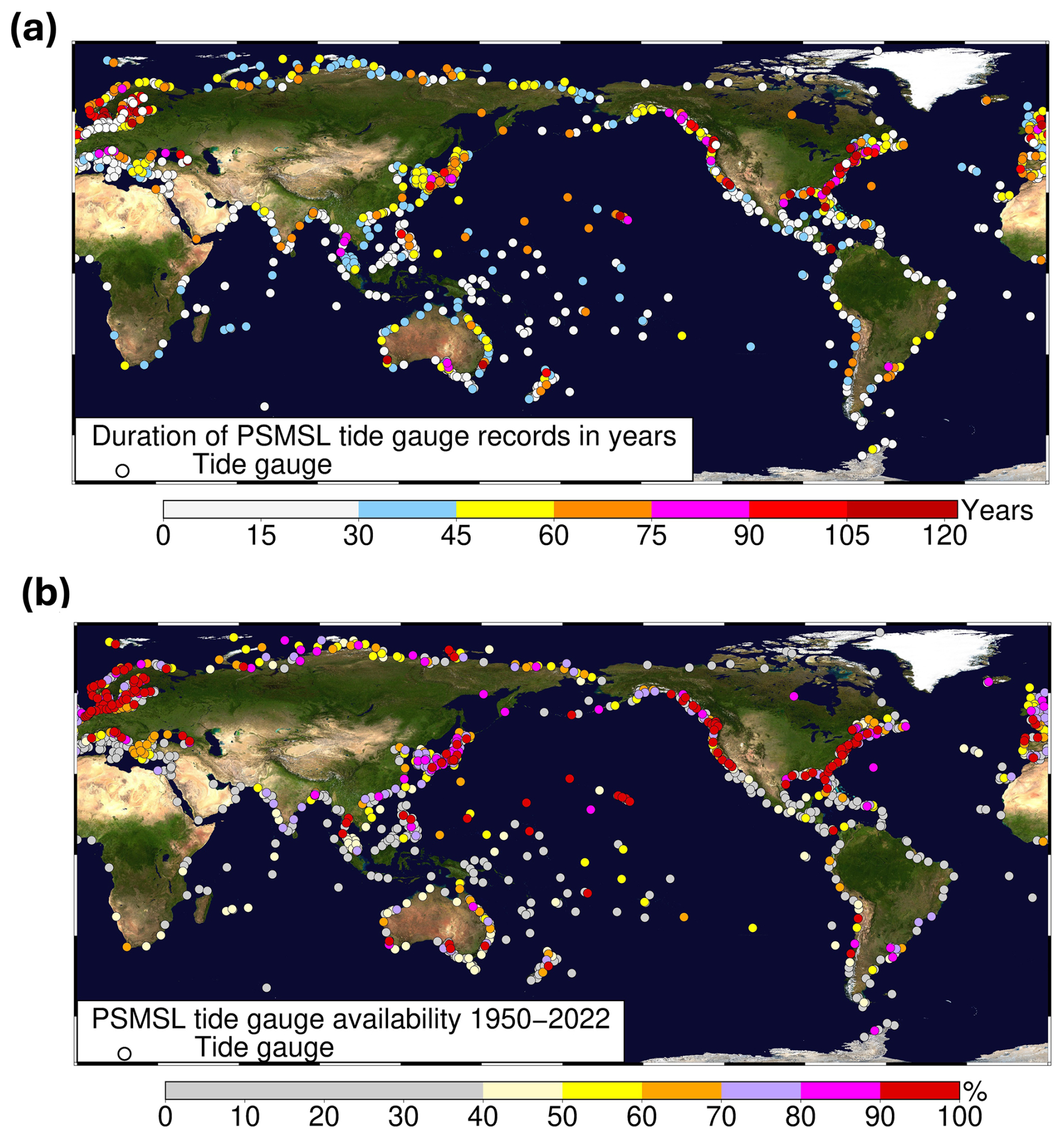
Figure 1 Global distribution of PSMSL (Permanent Service for Mean Sea Level) tide-gauge stations (a total of 1537 stations). (a) Stations colored by record duration (in full years). Ratio of stations in each duration range: ≤ 30 years (787/1537), 30–45 years (258/1537), 45–60 years (221/1537), 60–75 years (118/1537), 75–90 years (51/1537), 90–105 years (41/1537), 105–120 years (26/1537), ≥120 years (35/1537). (b) Percentage of each station's record available within 1950–2022. Ratio of stations in each completeness percentage range: ≤ 40 % (801/1537), 40 %–50 % (156/1537), 50 %–60 % (114/1537), 60 %–70 % (117/1537), 70 %–80 % (117/1537), 80 %–90 % (78/1537), ≥ 90 % (154/1537). Base map image: NASA (National Aeronautics and Space Administration) Blue Marble.

The spatial distribution of tide gauge records is crucial for accurate sea level reconstruction (Mu et al., 2018), and the number of gauges used significantly affects the ability of spatiotemporal analysis to capture the true spatial patterns (Calafat and Gomis, 2009; Cazenave et al., 2022). However, unexpected data gaps and uneven global distribution of tide gauge locations significantly impede the accuracy of sea level reconstruction and analysis (Meyssignac et al., 2012). To address the issue, three statistical methodologies have been tested: Autoregressive (AR) modeling, Probabilistic Principal Component Analysis (PPCA), and Regularized Expectation Maximization (EM). AR modeling uses linear combinations of nearby data points to interpolate missing values, refined through a method that balances estimates by weighted averaging of forward and backward filling (Akaike, 1969; Kay, 1988; Orfanidis, 2007). PPCA handles gaps within high-dimensional and noisy datasets by estimating latent variables and refining model parameters through covariance analysis, thus mitigating the effect of missing data and reconstructing to minimize data gaps (Roweis, 1998; Ilin and Raiko, 2010). Regularized EM directly estimates missing values through multivariable regression and iteratively augments model parameters, incorporating regularization to avert overfitting (Schneider, 2001). These methodologies collectively aim to enhance the accuracy of data gap filling by integrating observations using statistical methods. The effectiveness of the three methods to improve data continuity and thus the accuracy of tide gauge records is evaluated using numerical simulations.

The simulation study selected 48 near-complete (average data-missing rate 1.1 %) global long-term tide-gauge records (864 months; span from beginning of 1950 to end of 2021) from the PSMSL (Permanent Service for Mean Sea Level) Revised Local Reference (RLR) monthly product (Holgate et al., 2013) to evaluate the performance of different gap-filling methods for dealing with gaps in multi-decadal gauge data. To assess various data gap-filling methodologies corresponding to different data loss scenarios, these records are categorized into three groups, each subjected to varying levels of data gaps. Group 1 consists of 10 tide gauge records, each with three randomly generated gaps of different lengths – 12, 36, and 108 consecutive months. Group 2 includes a set of 10 records with the same configuration of random gap lengths as in Group 1, but with an additional 120 randomly missing single months dispersed throughout the entire simulated data record. Group 3 comprises 28 records, each missing 120 randomly selected single months of data. The spatial distribution of each group is illustrated in Fig. 2a. The efficacy of the three data gap-filling techniques on each of the simulated tide gauge records is evaluated based on the resulting gap-filled time series (Fig. S1–S3 in the Supplement).

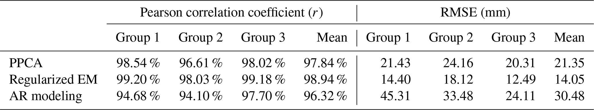
The numerical simulation experiment comparison summary (Fig. 2b and Table 1) shows that the Regularized EM algorithm consistently outperforms PPCA and AR modeling in all metrics. Notably, the regularized EM algorithm achieves an average correlation coefficient (r) of 0.99 with the observations, compared to 0.98 for PPCA and 0.96 for AR modeling across the 48 TG records. Regarding root mean square error (RMSE), the regularized EM method achieved an average RMSE of 14.05 mm, substantially lower than the 21.35 and 30.48 mm achieved by PPCA and AR modeling, respectively. Furthermore, a detailed analysis reveals that the Regularized EM algorithm also achieves the highest r and the lowest RMSE in each group compared to the other two methods, and the performance of the algorithm is relatively stable (in terms of r and RMSE) across the three groups, regardless of the type of missing data. To test generalizability, we used 198 tide-gauge records that are nearly missing-free over January 1980–December 2021, cropped all series to this common window, and repeated the gap-filling experiments. Using the three gap-filling methods, we imposed the three missing-data scenarios: (i) 40 gauges with a single contiguous gap of 12, 36, or 108 months; (ii) another 40 gauges with the same single-gap setting plus one random 120-month gap; and (iii) an additional 118 gauges with 120 months of random missing across the record. Performance was assessed against the complete (“true”) series. Full results are in Fig. S4 and Table S1. And results indicate Regularized EM again performs best across other methods – i.e., higher correlation coefficient and lower RMSE – and showing that the method ranking remains the same under a larger, more diverse test set.

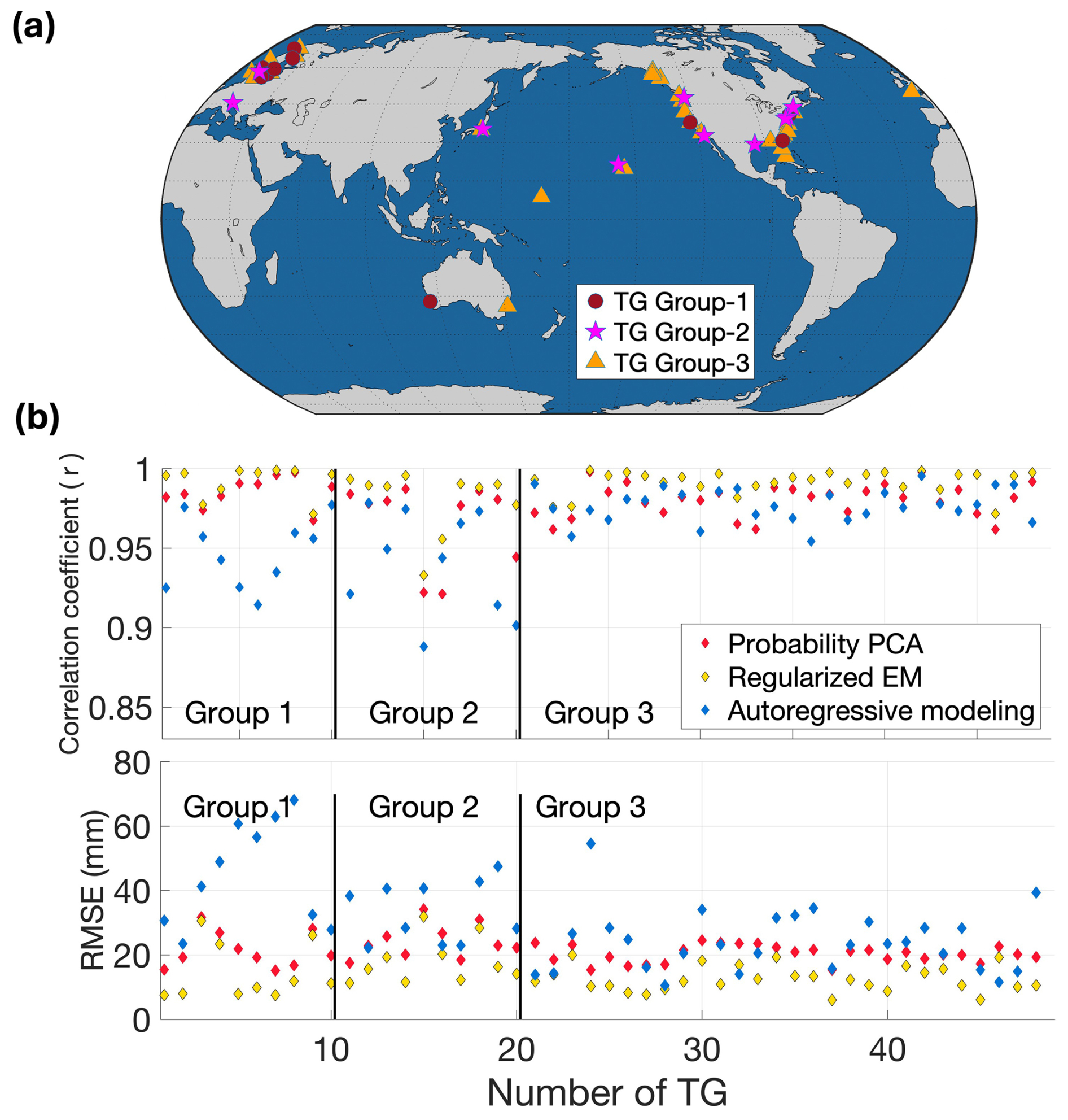
Figure 2 Spatial Distribution of the Tide Gauge (TG) records and validation of the three numerical simulation experiments. (a) Distribution of 48 nearly complete tide gauges used in the three simulations: Groups 1 and 2 each comprise 10 stations, and Group 3 includes 28 stations. (b) Correlation coefficients and RMSE between the gap-filled tide gauge records using the three methodologies (Probability PCA, Regularized EM, and Autoregressive Modeling), and the “true” observations in the simulation study. The Regularized EM method outperforms the other two methods.

Table 1 Comparing the performance of the three data gap-filling methodologies based on the average Pearson correlation coefficient (r) and Root Mean Square Errors (RMSE) between filled missing records and true observations in the simulation experiments.

In this study, the Regularized EM method is used to address data gaps in tide gauge records, resulting in a total of 287 global tide gauge records, compared to only 48 tide gauges before the data gap repairs. The tide gauge data spans from January 1950 through January 2022, and the locations of the tide gauges are shown in Fig. S5.

2.2 Alignments between satellite altimetry and tide gauge sea level records

Satellite radar altimetry has enabled global sea level measurements over the past three decades. The available data products include the Archiving, Validation, and Interpretation of Satellite Oceanographic (AVISO) data, European Space Agency's Climate Change Initiative (CCI), the Commonwealth Scientific and Industrial Research Organisation (CSIRO), NASA, the National Oceanic and Atmospheric Administration's Laboratory for Satellite Altimetry, the European Organisation for the Exploitation of Meteorological Satellites, the University of Colorado (CU), and Delft University of Technology. These organizations generate synchronized, validated, and consistent global sea level data products.

Multiple comparisons between altimetry sea level datasets from different institutions have been conducted. Wöppelmann and Marcos (2016) revealed that the AVISO gridded altimetry sea level strongly correlates with tide gauge records after removing linear trends and seasonality. Comparisons between satellite altimetry and tide gauge sea level records reveal that CCI and GSFC (Goddard Space Flight Center) data products have a median correlation of 0.7, CSIRO at 0.6, CU at 0.4, and AVISO leading with 0.8, following this, we use AVISO Level 4 monthly gridded sea level product (SSALTO/DUACS, 2022), January 1993–December 2021, for our study. To further account for potential TOPEX-A drift, we align the AVISO-based global mean sea-level estimates from January 1993 to February 1999 with the multi-mission record from TOPEX/Poseidon, Jason-1/-2/-3, and Sentinel-6 (version 5.2 GMSL product from PO.DAAC; Beckley et al., 2024), and apply the resulting difference uniformly across each grid.

Before combining altimetry and tide gauge records, it is essential to ensure consistency between these two types of measurements. An inverse barometer correction model, using ocean pressure data products from the National Centers for Environmental Prediction (NCEP-NCAR Reanalysis 1 provided by the NOAA Physical Sciences Laboratory, Boulder, Colorado, USA, Kalnay et al., 1996) applied to the tide gauge record, follows the correction method detailed in Ponte (2006), to allow approximate consistency with altimetry sea level data, which are corrected using the dynamic atmospheric correction. Knowledge of vertical land motion is necessary to convert the tide gauge records (of relative sea level change) to the geocentric (or absolute) sea level change time series associated with satellite altimetry (Kuo et al., 2004). Equation (1) denotes the relationship between altimetry geocentric sea level and tide gauge relative sea level, ignoring systematic errors, such as waves and others (Abessolo et al., 2023; Ray et al., 2023):

$$\begin{array}{}\text{(1)}& {\mathrm{SL}}_{\mathrm{SA}}={\mathrm{RSL}}_{\mathrm{TG}}+\mathrm{VLM}\end{array}$$

where:

$$\begin{array}{rl}& {\mathrm{SL}}_{\mathrm{SA}}:\text{Geocentric sea level from satellite altimetry}\\ & {\mathrm{RSL}}_{\mathrm{TG}}:\text{Relative sea level from tide gauges}\\ & \mathrm{VLM}:\text{Vertical land motions}\end{array}$$

Contemporary approaches for estimating vertical land motion (VLM) at tide-gauge sites include applying glacial isostatic adjustment (GIA) models, using Global Navigation Satellite System (GNSS) observations, and deriving rates from the satellite altimetry minus tide gauge (SA–TG) difference; we will first briefly discuss these methods and subsequently select the approach that is appropriate for our study. In many prior studies on sea level reconstructions, GIA models are used to correct the GIA-related long-term vertical land motion at tide-gauge sites, thereby making tide-gauge relative sea level more consistent with geocentric sea level from satellite altimetry (e.g., Church et al., 2004; Church and White, 2006, 2011; Hamlington et al., 2011, 2014; Meyssignac et al., 2012; Calafat et al., 2014), and assuming GIA is the only geophysical cause of vertical motion at tide gauge locations. This is a reasonable assumption in many regions, but for tide gauges affected by coseismic and postseismic displacements, it is only an approximation (Caccamise, 2019; Bevis et al., 2019). Contemporary 1-D or laterally varying 3-D GIA models, constrained by respective model-specific assumptions, have errors or could introduce systematic biases (King et al., 2012; Jevrejeva et al., 2014; Oelsmann et al., 2021). In addition, GIA geophysical process is not the only nor is it dominant everywhere on Earth for the origin of vertical land motion at tide gauge locations, including tectonics, erosion (Wöppelmann and Marcos, 2016), anthropogenic groundwater/mineral pumping, sediment load, and other deeper geodynamics other than GIA.

Global Navigation Satellite System (GNSS) can provide VLM estimates at collocated gauges, but in practice, its utility is limited by the scarcity of long, stable records (Wöppelmann et al., 2019) and influenced by long-period geophysical signals (Santamaría-Gómez and Mémin, 2015; Santamaría-Gómez et al., 2017). Additionally, in some regions, even minor geographic misalignments (a few kilometers) between the GNSS receiver and tide gauge can cause GNSS-estimated vertical land motion to inadequately represent gauge location motions due to the high spatial variability (Bevis et al., 2002; Oelsmann et al., 2021). Precise leveling provides an accurate tie, but it is labor-intensive and rarely maintained.

Other methods to estimate VLM have used the satellite altimetry minus tide gauge (SA–TG) approach (Nerem and Mitchum, 2002; Kuo et al., 2004; Kuo et al., 2008; Ray et al., 2010; Wan, 2015; Wöppelmann and Marcos, 2016; Oelsmann et al., 2021). In particular, Kuo et al. (2004, 2008) applied a network adjustment to reduce VLM error estimates to < 0.5 mm yr⁻¹ in semi-enclosed seas and lakes. Wan (2015) jointly solved for geocentric sea-level trend and VLM at global tide gauges. Wöppelmann and Marcos (2016) further showed that accurate VLM estimation via SA–TG requires a common data span of ≥ 20 years between altimetry and tide gauge data – a criterion that has been met.

The use of SA–TG methods to “correct” the same tide gauge records for land motion inevitably entails circular logic or tautological reasoning. Corrections are normally based on the introduction of independent or external information. A better way of describing the procedure used in this study is that we adjust the relative sea level histories recorded so that the sea level rate (post-adjustment) matches the estimate inferred nearby from satellite altimetry during the same (shared or common) time period of observation – a little less than 30 years. We can certainly view this adjustment as accounting for VLM. But this rate change is better thought of as an estimate of VLM rate, rather than a VLM `correction'. Having estimated the VLM rate in this way, we can apply this rate adjustment to the entire tide gauge data span, not just that part of the time series used to estimate the rate adjustment. The procedure makes an implicit assumption: that the rate of VLM during the entire time of the tide gauge (72 years) does not differ from the rate of VLM during the nearly 30-year period in which both altimetry and tide gauge data are available. This method presumes that long-term variations in vertical land motion (e.g., longer than 20–30 years) are negligible (which may not be reasonable when the tide gauge has been displaced by very large earthquakes). It further assumes that vertical land motion at most tide gauge locations is not significantly non-linear.

From a temporal perspective, GIA models represent deformation over centennial to millennial timescales (≈ 250–1000 years; Peltier, 2004; Stuhne and Peltier, 2015). While GNSS offers high temporal resolution, its spatial coverage and temporal span remain limited, with fewer than 20 sites possessing collocated records exceeding 29 years (SONEL, 2024, https://www.sonel.org/-GPS-.html, last access: 12 December 2024). Given these constraints, we adopt the SA–TG method – based on a 29-year overlap between satellite altimetry and tide gauge records – for estimating VLM at tide gauge locations in this study, subject to the assumptions discussed above.

To evaluate the efficacy of the SA–TG approach for VLM estimates, we used observed GNSS vertical motion at tide gauges from Hammond et al. (2021). Acknowledging the constraints of GNSS-derived VLM at tide gauge locations, as highlighted in studies such as Santamaría-Gómez et al. (2017), Wöppelmann et al. (2019), and Oelsmann et al. (2021), which scrutinized the spatial discrepancy between tide gauges and GNSS stations, our analysis extends to testing the impact of VLM estimates from GNSS solution uncertainty perspectives. This study assessed VLM solutions for 256 out of 287 tide gauges covered by the AVISO altimetry product, which were evaluated and compared to the collocated GNSS solution delineated by Hammond et al. (2021). Due to the unsatisfactory GNSS-based VLM quality, as specified by the criteria established in Hammond et al. (2021), three GNSS locations were excluded, which were responsible for the top three most significant discrepancies compared to collocated SA–TG solutions. The remaining 253 locations are denoted by pentagrams in Fig. 3a. Note that GNSS and SA–TG based VLM rates have different minimum effective record length requirements – GNSS typically ≥ 3.5 years (e.g., Wöppelmann et al., 2009; Hammond et al., 2021) versus SA-TG ≥ ∼ 20 years (Wöppelmann and Marcos, 2016); all solutions shown in Fig. 3 satisfy these criteria.

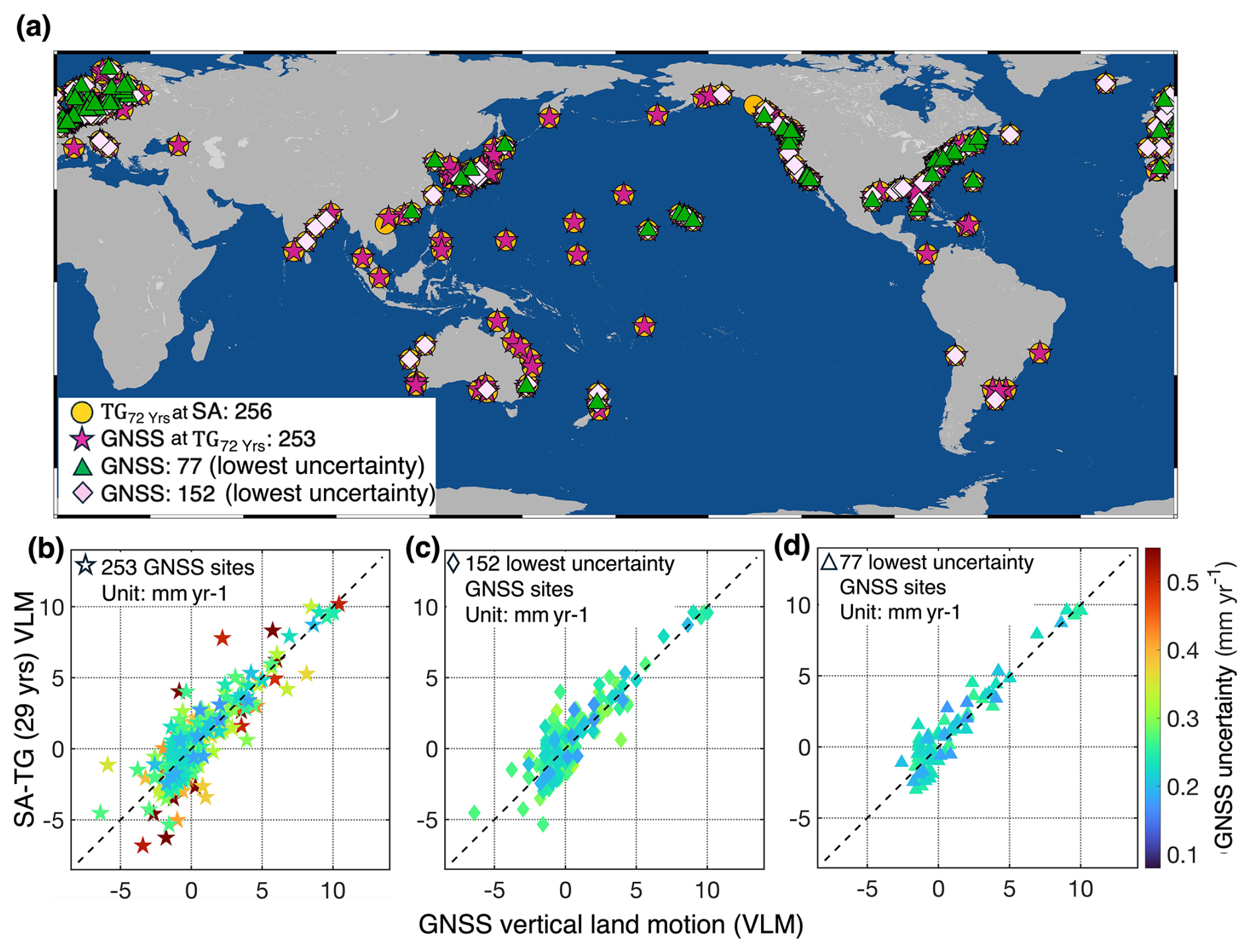
Figure 3 Comparison of vertical land motion estimates over 29 years from altimetry minus tide gauge (SA–TG) approach (this study) and the collocated GNSS solutions (Hammond et al., 2021). (a) 256 geographic locations using the SA–TG approach at the 72-year tide gauge locations (TG_72 years @SA), with 253 GNSS collocated at gauges (GNSS@TG_72 years) and the lowest 30 % and 60 % GNSS uncertainty locations (77 stations for the lowest 30 % and 152 stations for the lowest 60 %). (b) Vertical land motion estimates from 253 GNSS and collocated 29 years of data span the SA–TG approach, with color codes indicating the uncertainty value from GNSS measurements. (c) Vertical land motion estimates from the 152 locations with the lowest uncertainty GNSS and collocated SA–TG approach, highlighted with color-coded GNSS uncertainty. (d) Vertical land motion estimates from the 77 locations with the lowest GNSS uncertainty and collocated SA–TG approach, color-coded to represent GNSS uncertainty.

At 253 locations where GNSS and SA–TG are collocated (Fig. 3b), the two types of VLM rate estimates show a median (absolute) difference of 0.88 mm yr⁻¹ and correlate strongly with r= 0.86. The mean VLM rates estimated from 253 locations show 0.50 vs. 0.55 mm yr⁻¹ from GNSS and SA-TG approaches, respectively. Further analyses were conducted with the 152 GNSS solutions exhibiting the smallest uncertainties among the 253 GNSS-based solutions, with corresponding VLM rates shown in Fig. 3c. This subset exhibited a median difference of 0.81 mm yr⁻¹ and r= 0.89 between GNSS and SA–TG VLM (mean rate: 0.43 vs. 0.61 mm yr⁻¹) results. We also examined the 77 GNSS at tide gauge solutions with the smallest uncertainties. The GNSS and SA–TG VLM estimates (mean rate: 0.96 vs. 1.11 mm yr⁻¹) show a median difference of 0.64 mm yr⁻¹ and a r= 0.95 (Fig. 3d).

These results underscore that the lower GNSS uncertainties, VLM estimates are more closely aligned with the SA–TG approach despite not strictly conforming to the same temporal span between the two methods and without considering the minor geographical distances between GNSS and tide gauge locations.

Nevertheless, there does seem to be some systematic difference between VLM rates inferred from SA–TG and VLM rates measured using GNSS. We suggest that part of this difference results from reference frame realization error. That is, the reference frame (RF) used to express the GNSS stations' vertical velocities is not actually identical with the RF used to express geocentric sea level rates from altimetry. This phenomenon was discussed at some length in Bevis and Brown (2014) – two groups of geodesists trying to express velocities in the same RF (nominally) quite often fail to do so, particularly when they are working with different combinations of geodetic stations, and using different analysis methods. We estimate the VLM rate for each 72-year tide gauge record as the linear trend difference between the IB-corrected gauge records and the nearest (≤ 100 km) altimetry sea level measurements over January 1993–December 2021. We then add this constant VLM rate to the entire tide-gauge record to express it in the geocentric (altimetry) reference frame. Note that our procedure of transforming the tide gauge time series so as to adjust it onto an altimetry time series at a nearby point is probably the surest way to get both sea level time series expressed in the same RF.

In addition to applying the inverse barometer (IB) correction and adjusting site-specific VLM using the SA–TG approach, we performed a fast Fourier transform-based residual analysis to further align tide gauge and altimetry sea level variability for the stations used in the reconstruction. From an initial pool of 287 stations, constrained within 100 km of a gridded reference point, a subset was further excluded to mitigate redundancy in densely covered regions (e.g., northwestern Europe, Japan, North America), leaving 225 stations (Fig. S5). By analyzing the residual across the 225 stations, beyond seasonal harmonics (3 months, 6 months, and 12 months periods), two longer period signals – approximately 7.25 and 14.5 years – consistently emerged at most sites. These may be interpreted as manifestations of the known ∼ 6-year oscillation (Ding and Chao, 2018; Pfeffer et al., 2023) and the recently identified ∼ 13.6-year signal in GNSS VLM time series (Ding and Jiang, 2024), with the slight difference in periods potentially reflecting other geophysical processes. Incorporating this harmonic correction improved the agreement between altimetry and tide gauge records across the 225 sites.

This alignment step introduces a minimal bias, with the absolute difference in the mean sea level trend between the 225 processed tide gauges and the collocated altimetry measurements being as small as 0.02 mm yr⁻¹ over January 1993 to December 2021. Given its magnitude, we do not distinguish whether the harmonic correction is applied before or after the linear VLM adjustment within the tide gauge processing workflow. Moreover, this correction was not applied to the tide gauge records that were not used in the reconstruction process for independent validation to maintain consistency with previous studies. Notably, the tide gauges used in the reconstruction throughout each month remain fixed, thereby preserving more sites for subsequent independent validation.

2.3 Modified sea level reconstruction by combining CSEOF and EOF

Empirical Orthogonal Function (EOF) is a multivariate statistical technique extensively used for spatiotemporal analyses in atmospheric science, oceanography, and climatology. A notable variant, the Cyclostationary EOF (CSEOF), as described by Kim and North (1997), is particularly adept at analyzing climate time series characterized by dominant periodic oscillations by integrating a nested periodicity. In sea level studies, a 12-month cycle is commonly used to adeptly capture annual variations (Hamlington et al., 2011; Hamlington et al., 2013; Feng et al., 2024). Both EOF analysis and CSEOF are instrumental for understanding sea level variability. In the cyclostationary framework, an observed altimetry sea level anomaly X_i,j (with spatial index i and time index j) is assumed to exhibit a nested period d. We decompose X_i,j into two parts:

$$\begin{array}{}\text{(2)}& X_{i,j}={\sum }_k{\mathit{\varphi }}_k(i,j)A_{k,j}\end{array}$$

where: X_i,j denotes the altimetry sea-level anomalies, ϕ_k(i,j) is the cyclostationary loading vectors (CSLVs) for mode k at spatial point i and time point j, A_k,j is the principal component (PC) for mode k at time j.

The index k labels the order of the modes. Since each cyclostationary loading vector (CSLV) captures a cyclostationary process with period d, the cyclostationary load vector is:

$$\begin{array}{}\text{(3)}& {\mathit{\varphi }}_k(i,j)={\mathit{\varphi }}_k(i,j+d)\end{array}$$

Likewise, the associated covariance function C is also periodic with period d:

$$\begin{array}{}\text{(4)}& C(i,j;i^{\prime }{j}^{\prime })=C(i,j+d;i^{\prime }{j}^{\prime }+d)\end{array}$$

To find the kth CSLVs ϕ_k(i,j) and the corresponding eigenvalue Λ_k solve the Karhunen-Loève type equation adapted for CSEOF:

$$\begin{array}{}\text{(5)}& C(i,j;i^{\prime },j^{\prime }){\mathit{\varphi }}_k(i^{\prime },j^{\prime })={\mathrm{\Lambda }}_k{\mathit{\varphi }}_k(i,j)\end{array}$$

with the extracted CSLVs from the altimetry sea level anomalies, combining the optimal interpolation (Kaplan et al., 2000) to fit the collocated long-term sea level measurements to extend the PCs up to the tide gauge records' temporal range. For algorithmic details and practical guidance on CSEOF, we direct readers to Kim and North (1997) and Kim et al. (2015) for tutorials and applications; applications to CSEOF-OI sea-level reconstruction can be found in Hamlington et al. (2011) and Hamlington et al. (2014). However, utilizing the CSEOF method to analyze spatiotemporal sea level reveals the windowing effect in CSEOF trend mode (Multiplication of CSLVs that explain most of the trend in the altimetry sea level anomalies and respective PC), as discussed by Hamlington et al. (2019). This effect exhibits elevated standard deviations at the start and end of extracted trend components, decreasing towards the middle.

To clarify this issue, we use CSEOF decomposition on AVISO altimetry sea level anomalies and estimate the regional average of the trend modes, as shown in Fig. 4. Notably, areas like Northern Europe from 1993 to 1997 and from 2015 to 2021 show significant edge effects, with intensity varying by region.

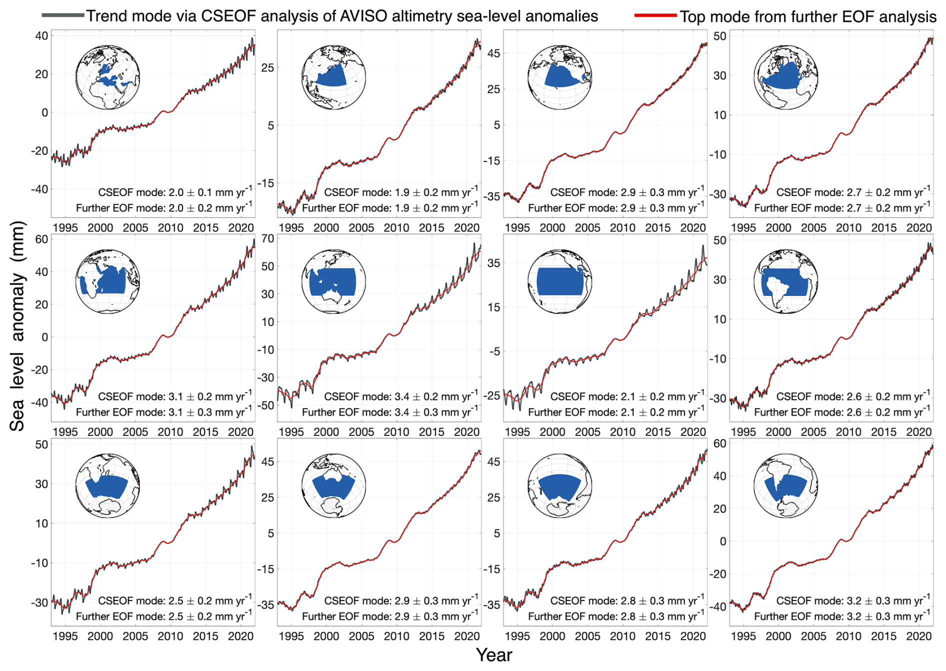
Figure 4 Identification of regional average trend mode in monthly AVISO altimetry sea level anomalies using CSEOF analysis. Subsequent EOF decomposition of these trend components has further delineated the primary component. The insets highlight the respective geographic study regions in blue. The values at the bottom of each panel report the fitted regional mean trends from the CSEOF trend mode and from the subsequent EOF mode, demonstrating their consistency.

When using CSLVs decomposed from 29-year altimetry sea-level anomalies and for reconstructing 72 years, the windowing effect can propagate to the entire reconstructed period through optimal interpolation (details in the upcoming section). To mitigate this issue, the study found further applying EOF decomposition to CSEOF trend mode X_trend, allowing for an accurate representation of nonlinear trends in altimetry sea level while eliminating portions that cause windowing effects (Fig. 4, red line). Specifically, it employs the first (EOF) principal component of X_trend denoted as $A_{\mathrm{trend}}^{*}$, along with its corresponding EOF spatial patterns ${\mathit{\varphi }}_{\mathrm{trend}}^{*}$ as further refine the CSEOF trend mode, denote as $X_{\mathrm{trend}}^{*}$.

$$\begin{array}{}\text{(6)}& {\displaystyle }{X}_{\mathrm{trend}}={\mathit{\varphi }}_{\mathrm{trend}}{A}_{\mathrm{trend}}\text{(7)}& {\displaystyle }{X}_{\mathrm{trend}}^{*}={\mathit{\varphi }}_{\mathrm{trend}}^{*}{A}_{\mathrm{trend}}^{*}\end{array}$$

The refined trend mode $X_{\mathrm{trend}}^{*}$ explains approximately 90 % of the variance in X_trend and accounts for about 13 % of the total variance in the gridded monthly AVISO altimetry sea level product (January 1993 to December 2021).

During the optimal interpolation, we integrated tide gauge records to extend the temporal coverage. Each tide gauge record is indexed by time t spanning from t=1 up to the entire duration of the records. For the top M CSLVs denote as ${\mathit{\varphi }}_{{\mathrm{CSEOF}}_M}$, after replacing the trend spatial pattern from CSEOF into the refined EOF spatial pattern, i.e., ${\mathit{\varphi }}_{\mathrm{trend}}^{*}$, we denote that the modified top M spatial patterns as ${\mathit{\varphi }}_{\mathrm{EOF}\mathit{\_}{\mathrm{CSEOF}}_M}$. Additionally, ${\mathit{\varphi }}_{{\mathrm{CSEOF}}_{N-M}}$ represents the high-order CSLVs obtained from altimetry sea level anomalies. Accordingly, we retain M=20, that is, ${\mathit{\varphi }}_{\mathrm{trend}}^{*}$ plus 19 additional CSLVs to capture 84 % of the variance in the 29-year AVISO dataset as fitted patterns, a choice guided by prior RSOI-based reconstruction configurations (Church et al., 2004; Church and White, 2006; Meyssignac et al., 2012; Hamlington et al., 2011).

We also investigated the impact of omitting the 1.4 % variance terms attributable to discrepancies between X_trend and $X_{\mathrm{trend}}^{*}$ during optimal interpolation. Our experiments indicate that excluding this part slightly improves the reconstruction performance, as evidenced by a marginally higher correlation between the observed altimetry global mean sea level (GMSL) and the reconstructed GMSL over the common dataspan. Therefore, we exclude this portion from the optimal interpolation (OI) computation. The overall reconstruction framework applied in this study is outlined through Eqs. (8)–(12), accompanied by detailed explanations.

$$\begin{array}{}\text{(8)}& {\displaystyle }\mathbf{R}=\mathbf{P}{\mathit{\varphi }}_{{\mathrm{CSEOF}}_{N-M}}{\mathbf{\Lambda }}_{{\mathrm{CSEOF}}_{N-M}}{\mathit{\varphi }}_{{\mathrm{CSEOF}}_{N-M}}^T{\mathbf{P}}^T+\mathbf{D}\text{(9)}& {\displaystyle }\begin{array}{rl}\mathbf{Q}& =\left({\mathit{\varphi }}_{\mathrm{EOF}\mathrm{\_}{\mathrm{CSEOF}}_M}^T{\mathbf{P}}^T{\mathbf{R}}^{-\mathrm{1}}\mathbf{P}{\mathit{\varphi }}_{\mathrm{EOF}\mathrm{\_}{\mathrm{CSEOF}}_M}\right.\\ & {\left.+{\mathbf{\Lambda }}_{\mathrm{EOF}\mathrm{\_}\mathrm{CSEOF}}^{-\mathrm{1}}\right)}^{-\mathrm{1}}\end{array}\text{(10)}& {\displaystyle }\begin{array}{rl}\mathrm{CovH}& ={\mathit{\varphi }}_{\mathrm{EOF}\mathrm{\_}{\mathrm{CSEOF}}_M}\mathbf{Q}{\mathit{\varphi }}_{\mathrm{EOF}\mathrm{\_}{\mathrm{CSEOF}}_M}^T\\ & +{\mathit{\varphi }}_{{\mathrm{CSEOF}}_{N-M}}{\mathbf{\Lambda }}_{{\mathrm{CSEOF}}_{N-M}}{\mathit{\varphi }}_{{\mathrm{CSEOF}}_{N-M}}^T+{\mathbf{H}}_{\mathit{ϵ}}\end{array}\text{(11)}& {\displaystyle }{\mathit{A}}_R=\mathbf{Q}{\mathit{\varphi }}_{\mathrm{EOF}\mathrm{\_}{\mathrm{CSEOF}}_M}^T{\mathbf{P}}^T{\mathbf{R}}^{-\mathrm{1}}{\mathit{X}}^{\mathrm{0}}\text{(12)}& {\displaystyle }\widehat{\mathit{x}}={\mathit{\varphi }}_{\mathrm{EOF}\mathrm{\_}{\mathrm{CSEOF}}_M}{\mathit{A}}_R\end{array}$$

For completeness, we include a brief implementation note describing the OI steps; detailed derivations follow Kaplan et al (2000). In Eq. (8), D denotes the instrumental error in tide gauge records. Wang et al. (2024) estimate D by applying 50 mm threshold to the first difference of records. In this study, we estimate D using a harmonic analysis is applied to periods guided by Bâki Iz (2014). For each gauge series, we fit sub- and super-harmonics along with a linear trend via least squares. The root mean square of the residuals between the fitted time series and observations is used to construct the D matrix, assuming that errors are independent across different tide gauge locations. The minimal instrumental error estimation is then set to the median of the resulting distribution to avoid overconfidence. Λ is the general notation describes the eigenvalues from different parts that are tagged at the bottom right of the symbol. Equation (9), where Q is a theoretical estimate for error covariance in the solution (Kaplan et al., 2000). Equation (10) CovH account for the error variance covariance matrix of the reconstructed field at each grid point, including large scale error (${\mathit{\varphi }}_{\mathrm{EOF}\mathrm{\_}{\mathrm{CSEOF}}_M}\mathbf{Q}{\mathit{\varphi }}_{\mathrm{EOF}\mathrm{\_}{\mathrm{CSEOF}}_M}^T$), high order error from CSEOF (${\mathit{\varphi }}_{{\mathrm{CSEOF}}_{N-M}}{\mathbf{\Lambda }}_{{\mathrm{CSEOF}}_{N-M}}{\mathit{\varphi }}_{{\mathrm{CSEOF}}_{N-M}}^T$) and the unfitted 1.4 % terms (H_ϵ). A_R (Eq. 11) represents extended PCs and $\widehat{\mathit{x}}$ (Eq. 12) describes the reconstructed gridded sea level anomalies.

Figure 5 illustrates the impact of windowing effects, as indicated by the elevated near beginning and end values in the moving standard deviation (STD) estimates of the CSEOF trend mode and their subsequent propagation following optimal interpolation. Further EOF decomposition of the CSEOF trend component shows a reduction in the edge amplitude of the moving STD, mitigating the tilting effect and propagation through extension and improving results after applying our modified reconstruction process. For simplicity, the combined approach of CSEOF, EOF, and optimal interpolation process will be referred to as the “Modified reconstruction” approach.

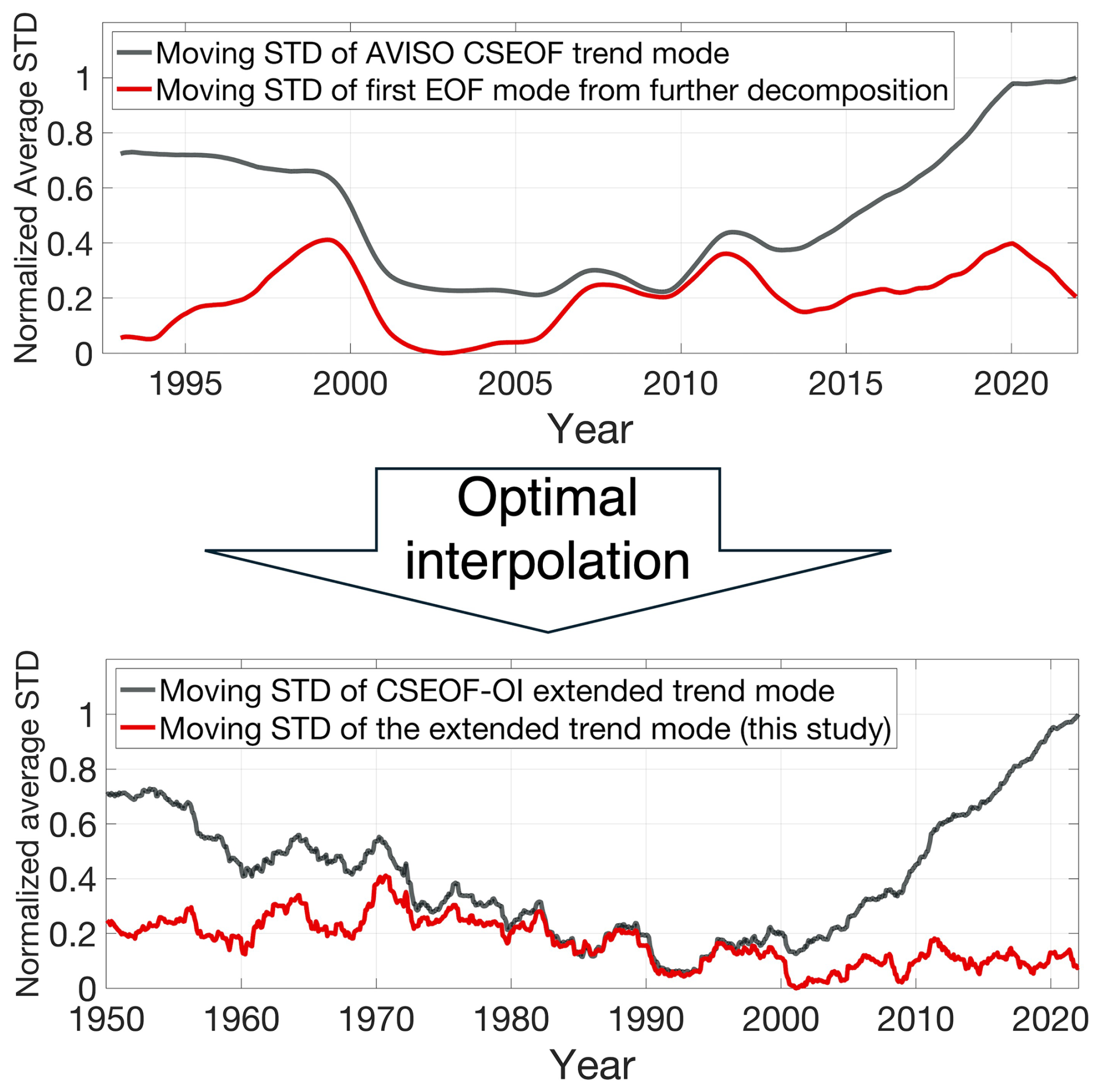
Figure 5 Top: Global average normalized standard deviations (STD) of AVISO altimetry sea level trend components via CSEOF (black) and the first component by further applying EOF (red). Bottom: STD from extended trend components using CSEOF-OI approach (black) and counterpart from modified reconstruction (red). 48-month window size on the estimate moving STD.

From the reconstructed sea level anomaly grids, $\widehat{\mathit{x}}$, we obtain the reconstructed global mean sea level at each time by aggregating over all grid points:

$$\begin{array}{}\text{(13)}& {\mathrm{GMSL}}_{\mathrm{OI}}=\mathit{w}\widehat{\mathit{x}}\end{array}$$

Where GMSL_OI represents the global mean sea level estimate from our modified reconstruction, and the w coefficients ensure that each spatial point of reconstructed sea level $\widehat{\mathit{x}}$ contributes proportionally to its area coverage. When CovH is the full covariance, the uncertainty in optimal interpolation reconstruction on global mean sea level, follows standard linear error propagation, where Var(⋅) stands for the variance operator.

$$\begin{array}{}\text{(14)}& \mathrm{Var}\left({\mathrm{GMSL}}_{\mathrm{OI}}\right)={\mathit{w}}^{\top }\mathrm{CovH}\mathit{w}\end{array}$$

However, in addition to this error, two additional sources of uncertainty can influence the resulting global mean sea level time series: (1) the error from the filling process for missing tide gauge records. (2) estimated VLM rate uncertainties at tide gauge locations.

To capture these effects, we conduct a Monte Carlo approach, generating multiple realizations (i.e., 300 times) of the gap-filled tide gauge dataset and the VLM-adjusted tide gauge dataset, respectively. Each realization is then passed through the optimal interpolation reconstruction in exactly the same way, producing an ensemble of global mean sea level.

From this ensemble, we compute two empirical standard deviations: σ_filling, quantifying the spread in global mean sea level arising from the gap filling uncertainty, and σ_VLM, reflecting the spread introduced by vertical land motion rate uncertainty.

If we regard these three components i.e. Var(GMSL_OI), ${\mathit{\sigma }}_{\mathrm{filling},}^{\mathrm{2}}$, and ${\mathit{\sigma }}_{\mathrm{VLM}}^{\mathrm{2}}$ as statistically independent, the total standard deviation can be approximated by:

$$\begin{array}{}\text{(15)}& {\mathit{\sigma }}_{\mathrm{GMSL}}\approx \sqrt{\mathrm{Var}\left({\mathrm{GMSL}}_{\mathrm{OI}}\right)+{\mathit{\sigma }}_{\mathrm{filling}}^{\mathrm{2}}+{\mathit{\sigma }}_{\mathrm{VLM}}^{\mathrm{2}}}\end{array}$$

We denote the per-grid uncertainty contributions from gap filling and from the VLM correction at time t as ${\mathit{\sigma }}_{{\widehat{x}}_{\mathrm{filling}}}\left(i,t\right)$ and ${\mathit{\sigma }}_{{\widehat{x}}_{\mathrm{VLM}}}\left(i,t\right)$, respectively, both are defined as the one standard deviation spread across the Monte-Carlo reconstructions in which the corresponding component is perturbed and the full reconstruction is rerun. Together with the error from the optimal interpolation process. The uncertainty for the i-th grid at time t can be represented as:

$$\begin{array}{}\text{(16)}& \begin{array}{rl}& {\mathit{\sigma }}_{\mathrm{regional}}\left(i,t\right)\approx \\ & \sqrt{\mathrm{CovH}(i,i,t)+{\left({\mathit{\sigma }}_{{\widehat{x}}_{\mathrm{filling}}}(i,t)\right)}^{\mathrm{2}}+{\left({\mathit{\sigma }}_{{\widehat{x}}_{\mathrm{VLM}}}(i,t)\right)}^{\mathrm{2}}}\end{array}\end{array}$$

To suppress short-term (≤ 3 months) fluctuations in the reconstructed sea level grids, we apply a low-pass finite impulse response (FIR) filter using a Blackman window with a sidelobe attenuation of −57 dB (Oppenheim and Schafer, 2010; Jwo et al., 2021). This procedure introduces a minor additional uncertainty, which is quantified based on the linear error propagation framework by Eichstädt et al. (2014). Although the filter-induced uncertainty is small relative to the total error budget, it is retained in our final estimates. Unless otherwise specified, all subsequent validations and analyses are based on the filtered reconstructions, including comparisons with altimetry and tide gauge records used for validation, both of which are processed using the same filter to ensure methodological consistency. For an overview of the modified reconstruction, see the schematic flowchart in Fig. S6.

3 Results

3.1 Validation

Sea level reconstructions leverage the extensive spatial coverage provided by altimetry measurements. Initial comparisons between the 29-year altimetry regional sea level trends (Fig. 6a) and those derived from the modified reconstruction (Fig. 6b) over the same period reveal a strikingly high correlation coefficient at r= 0.98.

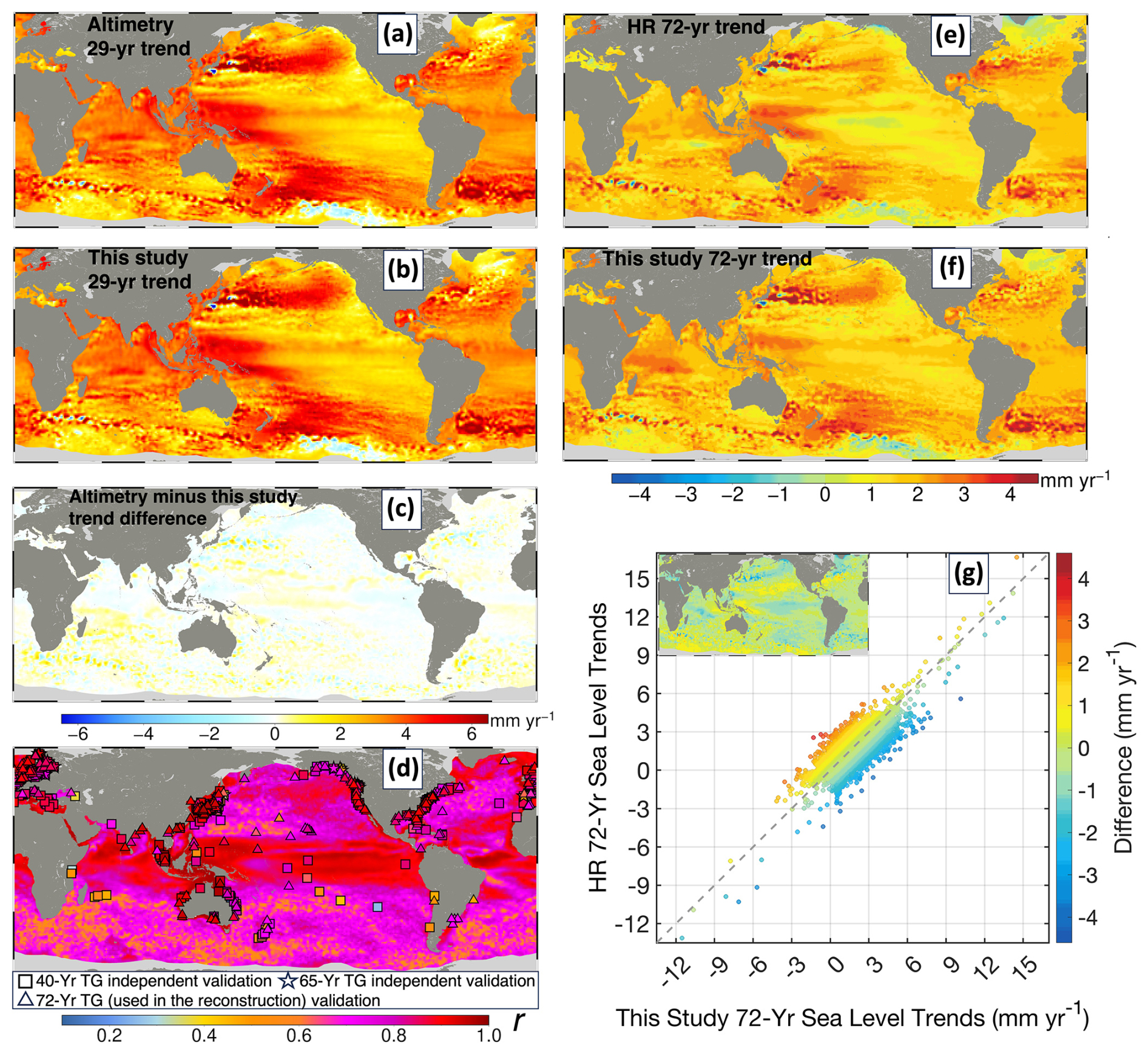
Figure 6 Validation of the modified sea-level reconstruction using multiple datasets. Panels (a) and (b) show the 29-year geocentric sea-level trends (January 1993–December 2021) from satellite altimetry measurements and the modified reconstruction, respectively, while panel (c) illustrates their difference; for altimetry-era trend consistency check, and the close similarity between (a) and (b) indicates that the reconstruction efficiently reproduces the altimetry-observed trend field. Panel (d) compares the detrended monthly modified reconstruction to two types of linear detrended tide gauge records not used in the reconstruction as long-term independent validations: 40-year series (January 1982–January 2022) from 224 stations (squares) and 65-year series (January 1957–January 2022) from 34 stations (pentagrams), and 225 stations (triangle) used in the reconstruction process spanning from January 1950 to January 2022. Shading indicates correlations between detrended altimetry and their respective reconstructions during January 1993–December 2021. Panels (e)–(f) depict regional geocentric sea-level trend over 1950–2021 from HR (Dangendorf et al. 2024, re-gridded at 1° × 1°) and from the modified reconstruction, (g) highlights the regional differences.

Figure 6c indicates that the differences in sea level trend estimates between altimetry and our reconstruction are minimal. The median absolute difference is 0.14 mm yr⁻¹, and 99 % of grid cells differ by no more than ±1 mm yr⁻¹. Considering that regional sea-level trends can exceed ±8 mm yr⁻¹ from 1993 to 2021, these small discrepancies underscore the high accuracy of the reconstruction in capturing altimetry-era trends.

The reconstructed global mean sea level trend estimates using ordinary least squares, adjusting for lag-1 autocorrelation, and incorporate additional reconstruction uncertainties via multiple realizations and re-fitting using Monte Carlo approach (Dangendorf et al., 2024), from the 29-year (January 1993 through December 2021) GMSL from modified reconstruction (3.2 ± 0.3 mm yr⁻¹, 95 % confidence) align with altimetry measurements (3.2 ± 0.3 mm yr⁻¹, 95 % confidence), underscoring the effectiveness in accurately capturing regional sea level trends during the altimetry era.

To assess how well the reconstruction captures sea-level variability, we computed the correlation coefficient (r) between linear detrended monthly sea levels at each grid point and collocated detrended altimetry measurements. The median r= 0.78, with most regions exceeding 0.7 and low-latitude equatorial areas consistently above 0.85 (Fig. 6d). Additionally, we validated the reconstruction using monthly tide gauge records (processed for fill missing data, IB, and VLM adjustment, followed by the previously described method) that were detrended and compared against nearby (≤ 200 km) reconstruction grids. This validation was performed over 40 years (January 1982 to January 2022; 224 gauges) and 65 years (January 1957 to January 2022; 34 gauges), yielding a consistent median r= 0.85 (85.24 % for 40 years and 84.70 % for 65 years). For gauges that were used in the reconstruction process (January 1950 to January 2022, 225 gauges), the results show a median r= 0.85 (84.76 %). The similar performance between gauges used in the reconstruction and those not used indicates a low risk of overfitting.

To evaluate regional sea level trends over the past seven decades, we compared our modified reconstruction using the HR reconstructed sea level available from Dangendorf et al. (2024). Known for superior trend estimation, the HR reconstruction outperforms other contemporary reconstructions in capturing long-term sea level trends (Dangendorf et al., 2019). Due to the spatial resolution difference between the two reconstruction products, we examine sea level trends from 1950 to 2021 across each 1° × 1° grid in various ocean basins by first resampling the products from Dangendorf et al. (2024) with the exact spatial resolution with our product, then hold the comparison across each grid (Within our 1° ocean grid, > 99.9 % of cells have a corresponding value in the re-gridded Dangendorf field), as detailed in Fig. 6e, f. Further analysis based on Figure 6g reveals that ∼ 40 % of the 1° × 1° grids exhibit discrepancies (absolute) below 0.30 mm yr⁻¹, while ∼ 80 % of the grids show discrepancies under 0.74 mm yr⁻¹, and ∼ 92 % maintain discrepancies less than 1 mm yr⁻¹. This demonstrates the efficacy of the modified reconstruction in capturing sea level trends both during and prior to the satellite altimetry era. Overall, these comparisons underscore the effectiveness of our modified reconstruction in accurately capturing both sea level trends and variabilities.

3.2 Climate pattern-induced sea level

Beyond high-frequency tidal components such as M2, S2, and O1 (Foreman, 1977), numerous low-frequency periodic irregular climate patterns are embedded within sea levels. Most research concentrates on regions particularly sensitive to specific climate modes, such as the Indian Ocean (Frankcombe et al., 2015; Kumar et al., 2020) and the Pacific Ocean (Si and Xu, 2014; Hamlington et al., 2016; Meng et al., 2019). Extracting global sea level responses to multiple climate patterns at the regional scale without relying on predefined climate indices remains complex. Although ENSO and PDO are recognized for their considerable influence on global sea level (Han et al., 2017), disentangling their individual effects accurately is particularly challenging due to their overlapping activity and spatiotemporal characteristics in the Pacific Ocean. Recognizing these challenges, this study believes that quality-enhanced sea level reconstructions could better quantify the significant climate pattern-induced sea level, including ENSO and PDO, thereby diminishing the reliance on predefined climate indices for pattern extraction.

Besides the improved reconstruction product, an effective decomposition method is essential for revealing physically meaningful spatiotemporal patterns. EOF analysis is widely applied to extract orthogonal modes of maximum variance; however, its performance may decline with compromised data quality, resulting in less coherent signals. By contrast, CSEOF incorporates cyclical variability by linking each mode with a PC and a periodic spatial pattern, although its strict periodic assumptions introduce artifacts in higher-order modes that may lack genuine cycles. To better capture higher-order variability, in this study, we use an EOF-based decomposition on our reconstructed sea level, while recognizing the value of CSEOF in sea level reconstructions.

Uncertainty in our EOF-based sea level patterns is estimated using a bootstrap approach (Wang et al., 2014). Each month in the time series is resampled with replacement to generate a synthetic dataset of equal size, preserving the overall observation count while randomizing the temporal order. Repeating this process 300 times yields an ensemble of EOF solutions. The standard deviation at each grid point across these solutions quantifies the spatial uncertainty, thus providing a nonparametric means of assessing how sensitive the extracted sea level patterns are.

Using EOF decomposition on the modified monthly sea level reconstruction from January 1950 to January 2022, the first component predominantly represents the trend and encompasses the annual variations, as illustrated in Fig. 7a–c. By testing the ability of this mode to represent the trends present in the reconstructed sea level, the study estimates the correlation coefficient of the EOF spatial pattern from the first mode and the 72-year geocentric sea level trend map. This analysis yielded a high correlation coefficient of r= 0.98. This highlights the overall trend representation of the first EOF mode, which accounts for 43 % of the overall variance of the 72-year monthly reconstructed sea level.

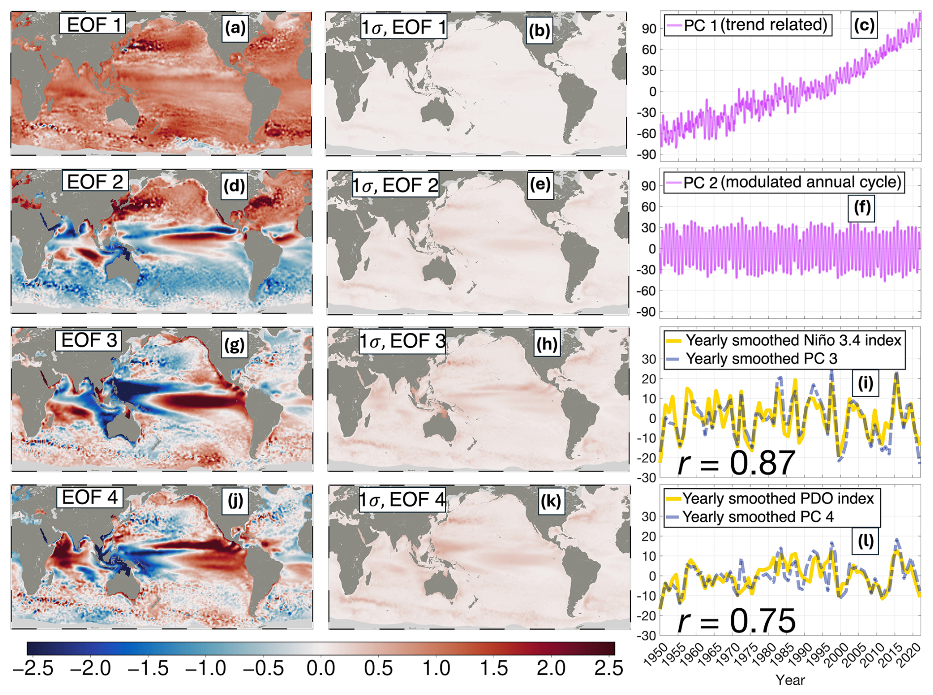
Figure 7 Top four EOF spatial patterns and their respective principal components (PCs) from the 72-year modified sea level reconstruction (this study), compared with the corresponding climate indices. Spatial pattern (a) and its corresponding uncertainty (b), together with PC (c) of the first EOF mode, exhibit a trend-related mode. The second EOF spatial pattern (d), pattern uncertainty (e), and its corresponding PC (f) represent the modulated annual cycle. The third EOF spatial pattern (g), respective pattern uncertainty (h), and corresponding yearly smoothed PC (i), which is closely linked to ENSO climate pattern, as evidenced by correlation with Niño 3.4 climate index (i) at r= 0.87 after yearly smooth. The fourth global EOF spatial pattern (j) and its uncertainty estimate (k), which is strongly related to PDO climate, is proven by a high correlation between the yearly smoothed PC 4 and respective PDO climate index (l) at r = 0.75. The Climate index scale matched with PCs, no additional detrending was applied.

The second EOF mode outlines the modulated annual cycle (MAC), highlighting a pronounced divergence between the northern and southern hemispheres due primarily to opposing seasonality (Fig. 7d). In the north hemisphere, mid- to high-latitudes exhibit a marked response to this mode, especially along the eastern coasts of China and Japan and the coastal regions of the United States. The uncertainty estimate (Fig. 7e) indicates a notable response on both sides of the equatorial Pacific, likely linked to ENSO. The corresponding PC 2 (Fig. 7f) confirms the annual oscillation in this component, which accounts for 12 % of the total variance.

The third EOF mode, derived from the modified 72-year reconstruction, corresponds to the El Niño–Southern Oscillation (ENSO). The Niño 3.4 index – defined based on sea surface temperature anomalies (SST) in the region 5° N–5° S, 170–120° W – is used as an ENSO indicator. The spatial pattern of EOF 3 (Fig. 7g) reveals a prominent positive sea-level anomaly in the central Pacific. Temporal characteristics are evaluated by correlating the third principal component (PC3) with the NOAA (https://psl.noaa.gov/data/timeseries/month/, last access: 20 May 2024) Niño 3.4 index (Fig. 7i). To mitigate high-frequency variability and emphasize interannual signals, both PC3 and the Niño 3.4 index are averaged annually and then interpolated back to a monthly (excluding January 2022), yielding a correlation of r= 0.87. Correlation significance was evaluated with a phase-randomized surrogate test (Ebisuzaki, 1997; N= 10 000). The annually smoothed PC3–Niño-3.4 correlation is statistically significant (p= 0.0001). The uncertainty estimate for EOF 3 (Fig. 7h) indicates elevated uncertainty along the eastern equatorial Pacific, the eastern coast of Mexico, and the Indian Ocean – regions strongly influenced by ENSO. This mode accounts for 7 % of the variance in the reconstructed sea levels, underscoring ENSO's significant impact on sea level.

The Pacific Decadal Oscillation (PDO) represents another key mode of climate variability in the Pacific, distinct from ENSO primarily in its temporal scale. Both phenomena arise from coupled ocean–atmosphere interactions, yet ENSO operates on seasonal to interannual timescales while the PDO unfolds over decadal periods. During a positive PDO phase, warmer SST prevail along the western North American coast and extend into the central Pacific, with cooler conditions in the northwest Pacific; these patterns reverse during a negative phase. The fourth EOF spatial pattern (Fig. 7j) from our modified reconstruction effectively captures these features, consistent with SST responses documented by Newman et al. (2016). Spatial uncertainty associated with this pattern is illustrated in Fig. 7k. The associated smoothed PC4 (Fig. 7l) exhibits a robust correlation (r= 0.75, p= 0.0001 at the surrogate tests) with the annually smoothed PDO index (https://ds.data.jma.go.jp/tcc/tcc/products/elnino/, last access: 20 May 2024) from the Japan Meteorological Agency (2024) (excluding January 2022), confirming its physical significance. This mode accounts for 5 % of the variance in the 72-year reconstructed sea level, underscoring the notable influence of the pattern.

EOF decomposition of 72 years of reconstructed monthly sea levels reveals that the first four modes, each linked to distinct physical processes, collectively account for approximately 68 % of the total variance. By capturing both trend and large-scale climate oscillations (e.g., ENSO and PDO) globally at the regional scale, these modes underscore the robust interpretability of our long-term reconstruction. Moreover, the approach quantifies physically significant sea-level patterns independently of external climate models or indices, thereby providing a self-consistent framework for assessing the roles of individual climate patterns in shaping sea level change.

To clearly compare our results with existing sea-level reconstructions, we conducted assessments using two independent datasets: the CSEOF-OI dataset (Hamlington et al., 2014) and the HR dataset (Dangendorf et al., 2024). The CSEOF-OI dataset, originally weekly-resolved from January 1950 to June 2009, was aggregated to the monthly resolution to match our analysis timeframe, treating the period from January 2009 to June 2009 as a full year to maximize comparability. The yearly HR dataset was truncated to cover the period 1950–2021, re-centered by removing the mean from each time series before EOF analysis, and its PCs were linearly interpolated to monthly values before comparison with corresponding climate indices. Both products adjusted their spatial coverage to best match our domain prior to the tests. In addition to the annual smoothing, a biennial smoothing was applied following a similar methodology: data were averaged over 24-month intervals, with the remaining length of 18 months or longer but less than 24 months treated as complete two-year intervals at the end, and the averaged values interpolated back to monthly resolution. Correlation coefficients between PCs and major climate indices are detailed in Table 2. Over the 72-year analysis, our reconstruction clearly distinguishes distinct PCs corresponding to individual climate patterns under both annual and 2-year smoothing scenarios.

Table 2 Summary of the strongest absolute correlation coefficients ($\left|r\right|$) between climate indices (ENSO and PDO) and principal components (PCs) derived from the EOF decomposition of sea-level reconstruction products. The analysis includes both 1-year and 2-year smoothed comparisons. Correlation values exceeding 0.7 are reported, as lower values are considered insignificant. For each case, the corresponding PC order is indicated in parentheses after the correlation coefficient.

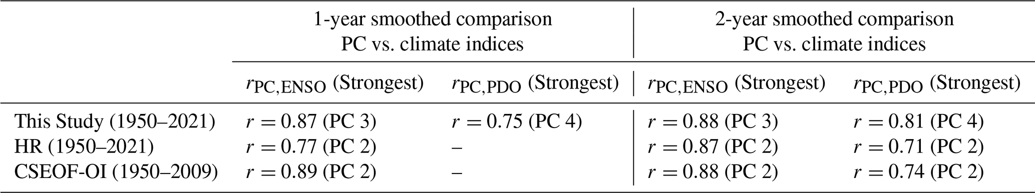
Over a 72-year span, our modified reconstruction consistently yields distinct, non-repeating PCs associated with individual climate patterns (i.e., PC 3 shows the strongest correlation with the Niño 3.4 index, and PC 4 with the PDO, indicating that these two dominant climate patterns are captured by distinct, non-overlapping EOF modes), as shown in both annual and 2-year smoothed scenarios.

At the annual smoothed case, the PCs from both the HR and CSEOF-OI products exhibit a clear representation of the ENSO pattern, with correlation values exceeding the r>0.7 threshold. The PDO-related correlations in the two products, suggest a less robust detection with no meeting the threshold. In the case of CSEOF-OI, this outcome may have been partly influenced by its slightly shorter time span (1950–2009).

Under the two-year smoothing, the HR product captures both ENSO and PDO signals, though they converge onto the same PC (PC2), with correlations of r= 0.87 and 0.71, respectively. A similar situation is found in the CSEOF-OI reconstruction, where PC2 also simultaneously reflects both Niño 3.4 and PDO (r= 0.88 and 0.74, respectively).

Among the tested products, our reconstruction demonstrates a consistent capacity to separate ENSO- and PDO-related signals into distinct PCs. This likely benefits from the enhanced sea level reconstruction achieved through the modified approach. Given the decadal to multi-decadal nature of the PDO, we anticipate that extending the temporal coverage of altimetry observations and sea level reconstructions in future studies will further enhance the separation of ENSO and PDO-induced sea level. While differing in focus and design, both the HR and CSEOF-OI approaches contribute valuable perspectives on ENSO-induced sea level.

3.3 Impacts of climate patterns on sea level changes

ENSO is characterized by sea surface temperature (SST) fluctuations lasting 2 to 7 years (Nicholls et al., 2007), whereas the PDO is a longer, irregular oscillation typically spanning 10 to 30 years (Mantua et al., 1997; Newman et al., 2016). To assess the simultaneous impacts of ENSO and PDO on sea level and mitigate high-frequency noise, we employ an analytical window spanning 5 years (61 months) across the dataset. Within each window, we fit a linear trend to the pattern-induced (i.e., the combined influence of ENSO and PDO) global mean sea level to better characterize their contributions.

Four intervals were selected, two of which fall within the satellite altimetry era (for validation purposes). For the pre-altimetry decades, the interval 1955–1960 exhibits a notable positive pattern-induced global mean sea level trend of 0.6 ± 0.4 mm yr⁻¹, while the 1988–1993 interval shows another prominent positive trend at 0.7 ± 0.4 mm yr⁻¹ . Within the altimetry period, the strongest negative pattern-induced global mean sea-level trend occurs during 1997–2002 (−1.0 ± 0.9 mm yr⁻¹), and the interval 2011–2016 records the highest positive contribution at 1.1 ± 0.5 mm yr⁻¹ .

Figure 8a illustrates regional sea-level trends from 1955 to 1960, revealing a pronounced rise along the equatorial eastern Pacific coast that extends northward toward Alaska and the Bering Strait, suggesting a combined influence of ENSO and PDO over this period. Elevated trends also appear in the southern Indian Ocean and east of Madagascar, whereas notable decreases occur offshore of northern Australia and east of the Philippines. Once the climate pattern–induced modes are removed (Fig. 8b), the prominent equatorial rise and mid- to high-latitude increases along the western coast of North America largely subside, and the previously strong signals in the Indian Ocean weaken. Likewise, the pronounced decline near Australia nearly disappears, underscoring the role of ENSO and PDO in shaping sea-level changes during this interval.

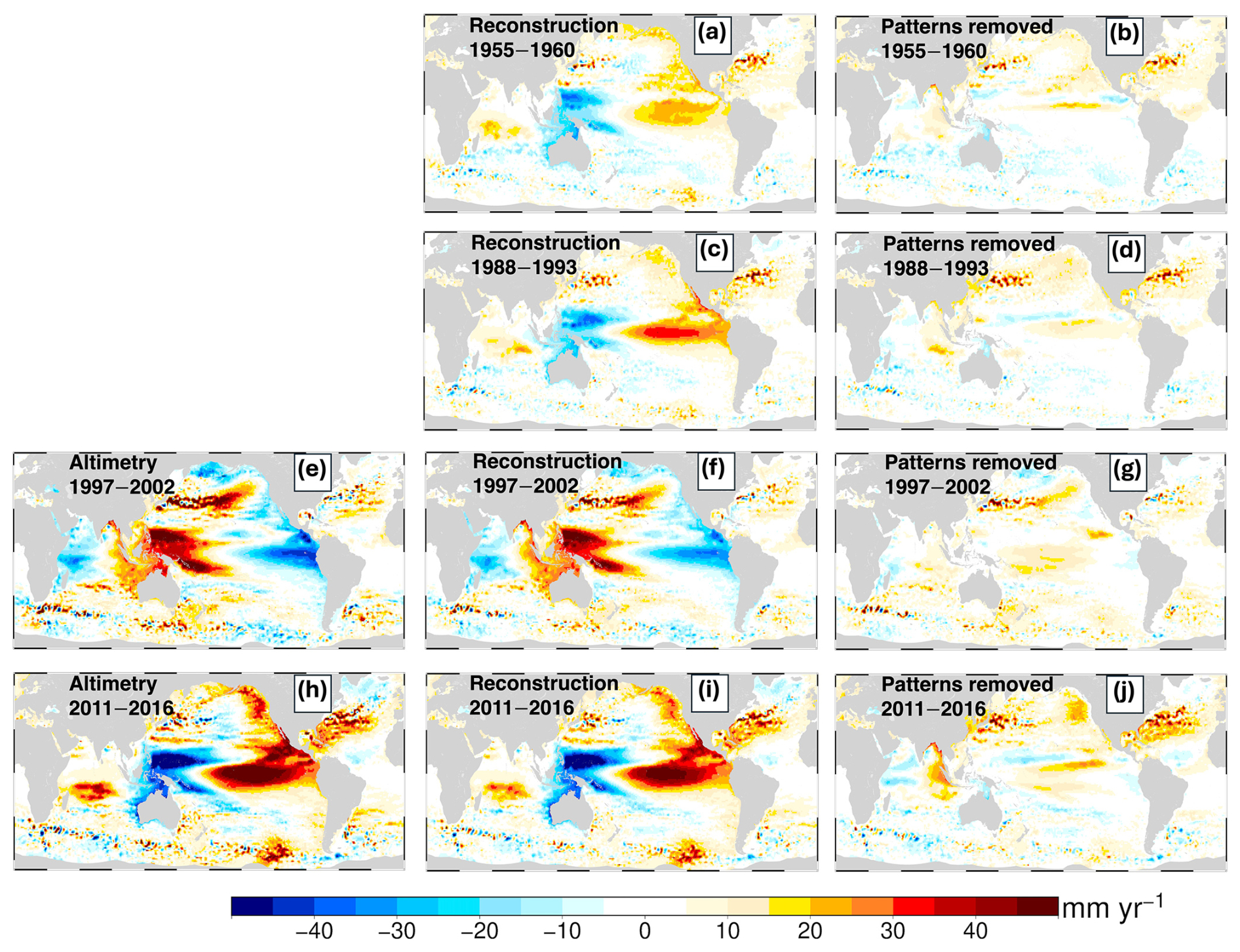
Figure 8 Comparative analysis of sea-level trends for four distinct five-year intervals: 1955–1960 (a, b), 1988–1993 (c, d), 1997–2002 (e, f, g), and 2011–2016 (h, i, j). Left-column panels (e, h) show altimetry-derived sea-level trends where available. Middle-column panels (a, c, f, i) depict sea-level trends from our modified reconstruction, while right-column panels (b, d, g, j) illustrate corresponding trends after removing ENSO- and PDO-related EOF modes. Color shading indicates the magnitude of sea-level trends (mm yr⁻¹). The altimetry-based trends correlate closely with our reconstruction, with r= 0.95 for 1997–2002 (e, f) and r= 0.97 for 2011–2016 (h, i), highlighting the effectiveness of our modified reconstruction in capturing short-term sea level trends.

During the interval from 1988 to 1993, regions exhibiting pronounced sea-level changes were predominantly concentrated near the equator, with limited influence at higher latitudes (Fig. 8c). According to ENSO classification (Trenberth, 1997), this period featured significant ENSO fluctuations, beginning with a strong La Niña event in 1988–89, which transitioned to a strong El Niño event from 1991 to 1992. These sequential ENSO phases resulted in marked regional contrasts: sea level notably increasing across the eastern Pacific, extending toward the International Date Line. Conversely, the western Pacific experienced significant sea-level declines concentrated primarily in mid- to low-latitude regions, consistent with typical ENSO-driven SST patterns (Yu and Kim, 2010). After removing ENSO and PDO signals (Fig. 8d), the trends in pattern active regions decreased from over ±35 mm yr⁻¹ to within ±10 mm yr⁻¹. Elsewhere, trends were generally within ±5 mm yr⁻¹, highlighting the dominant role of climate patterns in short-term sea level. However, compared to the scenario from 1955 to 1960, we found that the sea level rise during this five-year period mainly belongs to ENSO, as evident by the concentration of the strongest rising areas in the low-latitude Pacific.

From 1997 to 2002, a pronounced sea-level decline extended along the eastern Pacific Ocean into higher latitudes near the Bering Strait, coupled with widespread reductions across the Indian Ocean. Notably, the sea-level drop during this period exhibited a broader latitudinal range. Conversely, regions including Southeast Asia and eastern Japan experienced substantial sea-level increases, frequently surpassing 40 mm yr⁻¹, a pattern consistently captured by altimetry measurements (Fig. 8e) and our reconstruction (Fig. 8f). The strong regional correlation coefficient (r= 0.95) between the measured trends and our reconstructions confirms the method's effectiveness in capturing short-term fluctuations. These fluctuations reflect the prominent joint influence of ENSO and PDO, both notably active during this period, with clear declines appearing not only over the low-latitude Pacific but also near the Bering Strait. Once climate-induced EOF components are removed (Fig. 8g), the pronounced sea-level rises and declines largely diminish, with trends in most regions stabilizing within ±15 from ±45 mm yr⁻¹ .

During 2011–2016, altimetry measurements and our reconstruction reveal the most pronounced climate-induced positive sea-level trends of the altimetry era (Fig. 8h, i). Strongly positive trends dominate along the eastern Pacific coast and across the southern Indian Ocean, in contrast to significant declines along the low-latitude western Pacific coast. Notably, elevated sea-level anomalies are also evident along the eastern North Pacific and the West Antarctic Peninsula. These patterns are robustly confirmed by a correlation coefficient of r= 0.97 between altimetry measurements and trends estimated from our reconstruction. This expansive spatial coverage suggests simultaneous positive phases of both ENSO and PDO rather than dominance by a single climate pattern. After removing ENSO- and PDO-related components (Fig. 8j), most regional trends stabilize within ±20 mm yr⁻¹, substantially lower than uncorrected trends, which exceed ±50 mm yr⁻¹. However, residual variability persists in regions such as the North Atlantic and high-latitude areas along the western coast of North America, indicating potential influences from additional climate factors.

Analysis of extreme sea level events over the past 72 years reveals that the majority of interannual to decadal sea level changes cannot be attributed solely to ENSO dynamics; rather, the PDO also plays a significant role in most of the severe events we examined. This finding underscores the importance of considering both ENSO and PDO influences in understanding short-term sea level changes.

We further examined the influence of ENSO and PDO on longer-term sea-level changes and found that the pattern-induced sea-level trend during 1950–2021 is primarily localized in the equatorial Pacific, Southeast Asia, and parts of northern Australia (Fig. 9a). Regions such as northern Australia and the Gulf of Thailand exhibit negative trends of −0.8 to −0.5 mm yr⁻¹, while a limited area in the eastern equatorial Pacific shows positive trends of 0.8–1.0 mm yr⁻¹from the combined influences of ENSO and PDO over the past 72 years. The limited influence of pattern-induced sea level on long-term regional sea level trend is likely caused by the relatively short dominant periods of ENSO and PDO – shorter than half of the 72-year reconstruction period – thus limiting their large-scale influence. Additionally, we further estimated their effect on sea level acceleration. Given evidence of a ∼ 60-year oscillation in sea level (Chambers et al., 2012; Ding et al., 2021), we avoided directly comparing sea level acceleration coefficients before and after removing ENSO and PDO. Instead, we fitted the acceleration term of the pattern-induced sea level itself, enabling a clearer assessment of how these modes influence long-term sea-level acceleration.

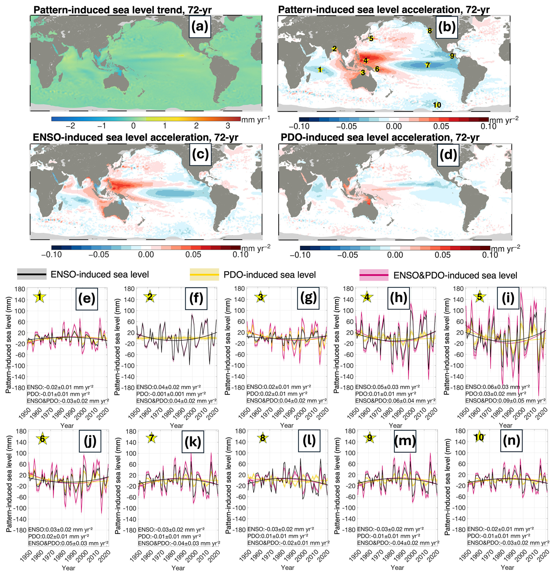
Figure 9 Pattern-induced sea-level trends and acceleration coefficients over the 72-year period (1950–2021). Panel (a) shows the combined ENSO- and PDO-induced regional sea-level trend, while panel (b) depicts the corresponding sea-level acceleration. Panels (c) and (d) illustrate the respective sea level acceleration coefficient contributed from the 72-year ENSO-induced sea level and the PDO-induced sea level, respectively. Highlighting representative locations marked by asterisks in panel (b) whose time series are provided in panels (e)–(n). In these time series, the individual and combined influences of ENSO and PDO are presented at annual resolution, and the curves represent quadratic fits, and 3σ error bars are derived from monthly pattern-induced sea-level errors via error propagation. Each panel (e–n) also reports the location-specific acceleration coefficient and its standard error at the bottom.

Unlike the pattern-induced sea-level trend of the past seven decades, the corresponding acceleration field shows a pronounced global imprint that resembles a superposition of ENSO- and PDO-like patterns (Fig. 9b). A notable negative response emerges in the eastern Indian Ocean, while positive anomalies appear in the Bay of Bengal and the Burmese Sea, extending along Australia's west coast. This positive influence further spans the entire western Pacific, with peaks in the equatorial region and the Kuroshio current area, where the acceleration coefficient reaches 0.06–0.09 mm yr⁻². Negative acceleration coefficients dominate the eastern Pacific, extending northward into the Gulf of Alaska and southward along the Peruvian coast, with an additional pronounced negative feature in the Amundsen Sea. The color scale is set to [−0.10, 0.10] mm yr⁻², which is approximately half the range previously estimated for regional sea-level acceleration since 1960 and 1970 (Dangendorf et al., 2019, 2024).

Furthermore, we visualize the pattern-induced sea level acceleration coefficients for ten representative locations that are strongly affected by these climate modes, in order to estimate their contributions to sea-level acceleration from ENSO and PDO separately as well as from their combined influence. This analysis is presented in Fig. 9e–n, with the ten locations marked by asterisks on the regional pattern-induced sea level acceleration map (Fig. 9b). The pattern-induced sea level is converted from monthly to yearly for a more accurate acceleration estimate. Error estimates are derived under the assumption that uncertainties originate solely from the spatial patterns of the EOF modes. The associated errors at each time step are then converted to a yearly error following error propagation.

Our analysis indicates that, in the majority of strongly responding regions, the acceleration effects induced by ENSO and PDO exhibit the same sign. However, in a few areas, the signals diverge. For example, along the western coast of North America, ENSO produces a negative acceleration of −0.03 ± 0.02 mm yr⁻², whereas PDO generates a positive feedback of 0.01 ± 0.01 mm yr⁻² (Fig. 9l). Moreover, among the ten visualized locations, ENSO consistently emerges as the dominant influence compared to PDO.

These results highlight that from a multi-decadal perspective, while the pattern-induced sea-level trend from ENSO and PDO remains relatively localized, the associated acceleration signals leave a broader global imprint over the past 72 years. Most notably, ENSO emerges as the dominant influence in most of the regions visualized, though PDO can either reinforce or counteract ENSO's effects. Such findings underscore the importance of accounting for multiple climate patterns when assessing both short-term sea-level variability and longer-term acceleration.

3.4 Sea level changes from 1950 to 2022

Upon validating our modified sea level reconstruction and explaining the role of ENSO and PDO in sea level changes, we estimate regional geocentric sea level trends from January 1950 to January 2022 by linearly fitting our reconstructed monthly product, which removed ENSO and PDO influence, as depicted in Fig. 10a. Since 1950, the Western Pacific region has exhibited notably higher sea level rise rates than other areas, typically ranging from 2.5 to 3.5 mm yr⁻¹ . Conversely, the equatorial eastern Pacific experiences lower rates, typically ranging between 1 to 2 mm yr⁻¹. Across the Atlantic Ocean, especially along the coastal regions of North and South America, sea level rise is more pronounced, commonly falling within 2 to 3 mm yr⁻¹ . The Indian Ocean shows moderate increases, averaging from 1.5 to 2.5 mm yr⁻¹. Certain areas west of the Antarctic Peninsula display negative trends, suggesting localized sea level declines.

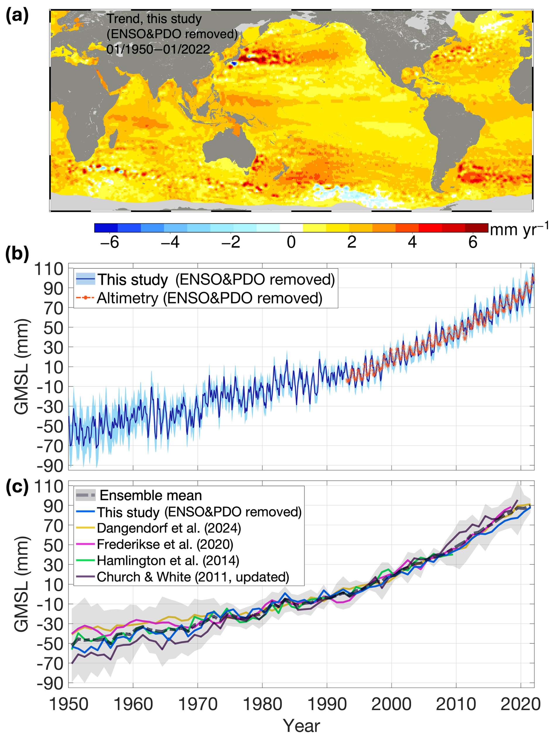
Figure 10 Reconstructed global geocentric sea-level trends and evolution since 1950. Panel (a) shows regional sea-level trends derived from our modified reconstruction, with ENSO- and PDO-induced sea level removed, spanning January 1950 to January 2022. Panel (b) presents the monthly global mean sea level (GMSL) time series from the same reconstruction, which removed ENSO and PDO influences, with 3σ error estimates for each time point, and compares it against altimetry-based GMSL that has also been corrected for ENSO and PDO using our spatiotemporal modes over the altimetry period. (c) Yearly GMSL since 1950, as obtained from the modified reconstruction and additional annual GMSL datasets (including an ensemble mean) with 3σ error estimate.

Due to the limited availability of high-frequency (e.g., monthly, weekly) sea level reconstruction products, we integrated data from various studies – each with different temporal resolutions – into yearly values to facilitate comparison, as illustrated in Fig. 10c. For studies that provide gridded datasets (e.g., Hamlington et al., 2014; Dangendorf et al., 2024), we adjusted their spatial coverage to best match ours before estimating their respective GMSL. The resulting comparisons are presented in Table 3.

Table 3 Global mean sea-level trend estimates from various studies since 1950. Error estimates account for uncertainties in global mean sea level. For modified reconstruction (This study), the trend was derived from monthly results, whereas all other estimates are based on yearly resolution.

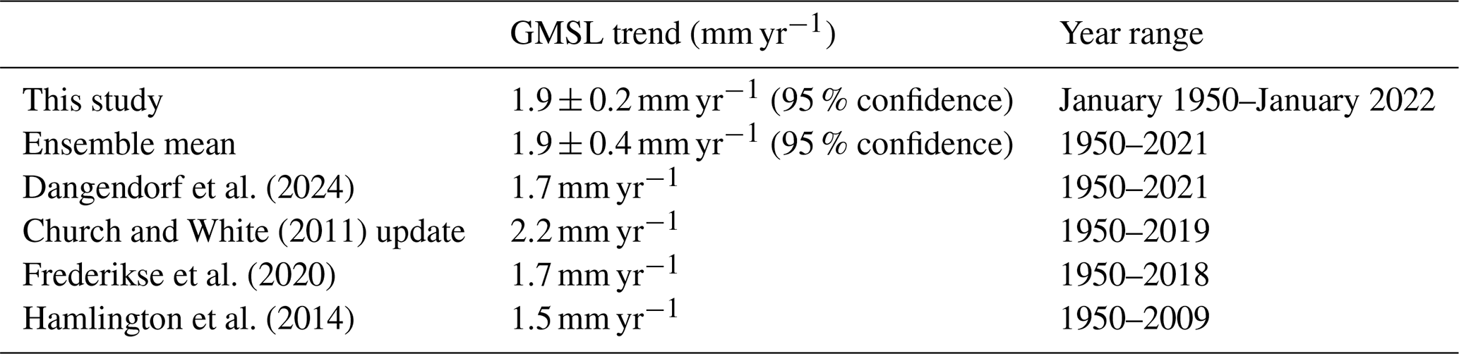
From January 1950 to January 2022, our modified sea-level reconstruction yields a global mean sea-level trend of 1.9 ± 0.2 mm yr⁻¹ (95 % confidence) after removing ENSO and PDO influences. This estimate closely aligns with the Ensemble Mean trend of 1.9 ± 0.4 mm yr⁻¹ (95 % confidence) for 1950–2021, and is comparable to 1.7 mm yr⁻¹ by estimating dataset from Dangendorf et al. (2024) and 1.7 mm yr⁻¹ by Frederikse et al. (2020) during 1950–2018. By contrast, Church and White (2011, update) yield the highest trend of 2.2 mm yr⁻¹ for 1950–2019, while Hamlington et al. (2014) report the lowest trend at 1.5 mm yr⁻¹, likely due to the exclusion of recent data (1950–2009). Overall, our global mean sea level estimate falls between the higher and lower values reported over the past 60–70 years. Despite methodological differences, all studies consistently indicate an increasing rate of sea-level rise over multiple decades. Furthermore, independent assessments consistently indicate that the global mean sea level trend during the past three decades (1993–2021; ≈ 3.2 mm yr⁻¹) is substantially higher than the estimated global mean sea level trend over the past seven decades.

4 Code and data availability

The gridded sea-level reconstruction products, including validation datasets, EOF analysis results, associated uncertainties, short-term sea-level trend fields before and after the removal of ENSO- and PDO-induced sea level, and pattern-induced contributions to long-term sea-level changes, along with additional supporting datasets, are publicly available at https://doi.org/10.5281/zenodo.15288816 (Wang, 2025). The gridded datasets are provided globally at a spatial resolution of 1° × 1°. To facilitate data usage, analysis, and plotting, scripts developed in MATLAB (for time series analyses) and Generic Mapping Tools (GMT; for spatial field visualizations) are also provided. Users are referred to the repository for accessing both the datasets and the associated visualization codes.

5 Discussion and Conclusion

Sea level change, driven by climate dynamics, presents scientific challenges (particularly in terms of reconstruction and prediction) and will produce profound impacts on global societies and economies. The current 29-year dataset derived from satellite altimetry is insufficient to capture long-term trends and discern the intricacies of internal oceanic variability that contribute to sea level rise over multi-decadal to century-long timescales. Conversely, long-term tide gauge records are hindered by scarcity and spatial unevenness. The integration of these two types of measurements enables reconstruction of the spatiotemporal long-term sea level. However, the deficiencies of tide gauge records and the temporal mismatches between the two types of measurements limit the quality of the reconstructed sea level. Our study tackles the issue of insufficient long-term tide gauge records by using the Regularized EM method, proven to be the most effective, to mitigate tide gauge record data gaps and increase the number of global tide records from 48 to 287, January 1950 through January 2022. Drawing on high-quality tide gauge records and altimetry sea level anomalies, we propose a modified sea level reconstruction method that integrates CSEOF and EOF to mitigate trend-related component windowing issues in the CSEOF process. The resulting reconstructed monthly sea level trend field strongly correlates with AVISO satellite altimetry (r= 0.98) over the overlapping period. Additionally, the reconstructed variability maintains a consistently high median correlation (r= 0.85) with collocated monthly tide gauge records that were not included in the reconstruction process across multiple decades, further validating its robustness.

Applying EOF decomposition to our 72-year sea-level reconstruction, we robustly isolate the ENSO-induced mode in agreement with prior studies. Moreover, the enhanced product captures PDO-induced sea level in a distinct EOF mode orthogonal to the ENSO mode, thereby providing a unified framework for separating and quantifying sea-level responses to these two major climate patterns without imposing predefined model constraints. The quantified pattern-induced modes reveal that both ENSO and PDO exert significant influences on sea level globally at the regional scale, and that ENSO alone may not be enough to explain certain sub-decadal fluctuations. Over the long term, the combined influences of ENSO and PDO substantially modulate sea-level acceleration over the past seven decades. Together with the trend-related and the modulated annual cycle EOF modes, these physically interpretable components account for 68 % of the variance in the reconstructed monthly sea-level fields over the full 72-year period.

In conclusion, our reconstructed 72-year sea level dataset provides a valuable resource for disentangling and clarifying the contributions of major climate patterns to sea level variability and trends. By enabling more accurate representation of oceanic signals, our product strengthens efforts to understand both short-term and long-term sea level changes.