Global emissions and abundances of chemically and radiatively important trace gases from the AGAGE network

Measurements from the Advanced Global Atmospheric Gases Experiment (AGAGE) combined with a global 12-box model of the atmosphere have long been used to estimate global emissions and surface mean mole fraction trends of atmospheric trace gases. Here, we present annually updated estimates of these global emissions and mole fraction trends for 42 compounds through 2023 measured by the AGAGE network, including chlorofluorocarbons, hydrochlorofluorocarbons, hydrofluorocarbons, perfluorocarbons, sulfur hexafluoride, nitrogen trifluoride, methane, nitrous oxide, and selected other compounds. The data sets are available at https://doi.org/10.5281/zenodo.15372480 (Western et al., 2025). We describe the methodology to derive global mole fraction and emissions trends, which includes the calculation of semihemispheric monthly mean mole fractions, the mechanics of the 12-box model and the inverse method that is used to estimate emissions from the observations and model. Finally, we present examples of the emissions and mole fraction data sets for the 42 compounds.

1 Introduction

Quantifying the global emissions of halogenated and other long-lived radiatively and chemically important trace gases is crucial for estimating their environmental impacts, such as depletion of the stratospheric ozone layer, and contributions to radiative forcing. Chlorofluorocarbons (CFCs), halons, and the solvents carbon tetrachloride (CCl₄) and methyl chloroform (CH₃CCl₃) are trace gases that have been phased out for emissive use under the Montreal Protocol on Substances that Deplete the Ozone Layer. Emissions of these gases persist because they are still contained within appliances, foams, and other applications, produced before their phase out, and continue to leak into the atmosphere. In some cases, production is ongoing because of their exempted production for chemical manufacture. Some of these substances remain in the atmosphere for years to centuries after they are emitted, owing to their long atmospheric lifetimes. Where non-ozone-depleting alternatives could not immediately be found, these gases were replaced by hydrochlorofluorocarbons (HCFCs), which are currently being phased out under the Montreal Protocol. HCFCs are in turn being replaced by hydrofluorocarbons (HFCs). While HFC do not deplete ozone, they have large global warming potentials, much like the ozone-depleting substances that they replaced. As a result, the production of HFCs is now being phased down under the Kigali Amendment to the Montreal Protocol. Chlorinated very short-lived substances (Cl-VSLS), with atmospheric lifetimes less than around six months, and some halomethanes, with both natural and anthropogenic sources, are not controlled under the Montreal Protocol and may present a threat to ozone layer recovery. Collectively, the controlled and uncontrolled ozone-depleting substances are responsible for almost all of the anthropogenic chlorine and bromine input to the stratosphere. There are a number of non-ozone depleting fluorocarbons that have extremely large global warming potentials, such as perfluorocarbons (PFCs), sulfur hexafluoride (SF₆) and nitrogen trifluoride (NF₃), and are almost entirely industrially produced. Halogenated substances, along with methane (CH₄), which critically affects the oxidative capacity of the atmosphere, and nitrous oxide (N₂O), which is also an ozone-depleting substance, are responsible for almost all the gaseous radiative forcing from anthropogenic sources beyond that of carbon dioxide. As a result, monitoring of these gases is crucial to understand the state of the atmosphere.

The Advanced Global Atmospheric Gases Experiment (AGAGE, Prinn et al., 2000, 2018) network publicly releases measurements of the dry-air mole fractions of 45 atmospheric compounds (Prinn et al., 2022). Measurements made through AGAGE and its predecessors (see Sect. 2) were initially used to derive atmospheric lifetimes of CFC-11, CFC-12 (Cunnold et al., 1983) and other trace gases, (e.g., Prinn et al., 1983a, 1995, 2005; Rigby et al., 2013; Thompson et al., 2024). However, the predominant use of AGAGE measurements currently is to estimate global emissions and mole fraction trends over time (Sect. 4). Here, we present global emissions and derived mole fraction trends for 42 trace gases (Table 1), inferred from AGAGE measurements and a 12-box model of the atmosphere (estimates are not provided for hydrogen, carbon monoxide and trichloroethene). We refer to these quantities as AGAGE-derived products, which are available at https://doi.org/10.5281/zenodo.15372480 (Western et al., 2025). The primary purpose of this article is to describe the methodology underpinning these AGAGE-derived products.

Table 1 Compounds measured by the AGAGE network for which emissions and atmospheric mole fraction trends are estimated.

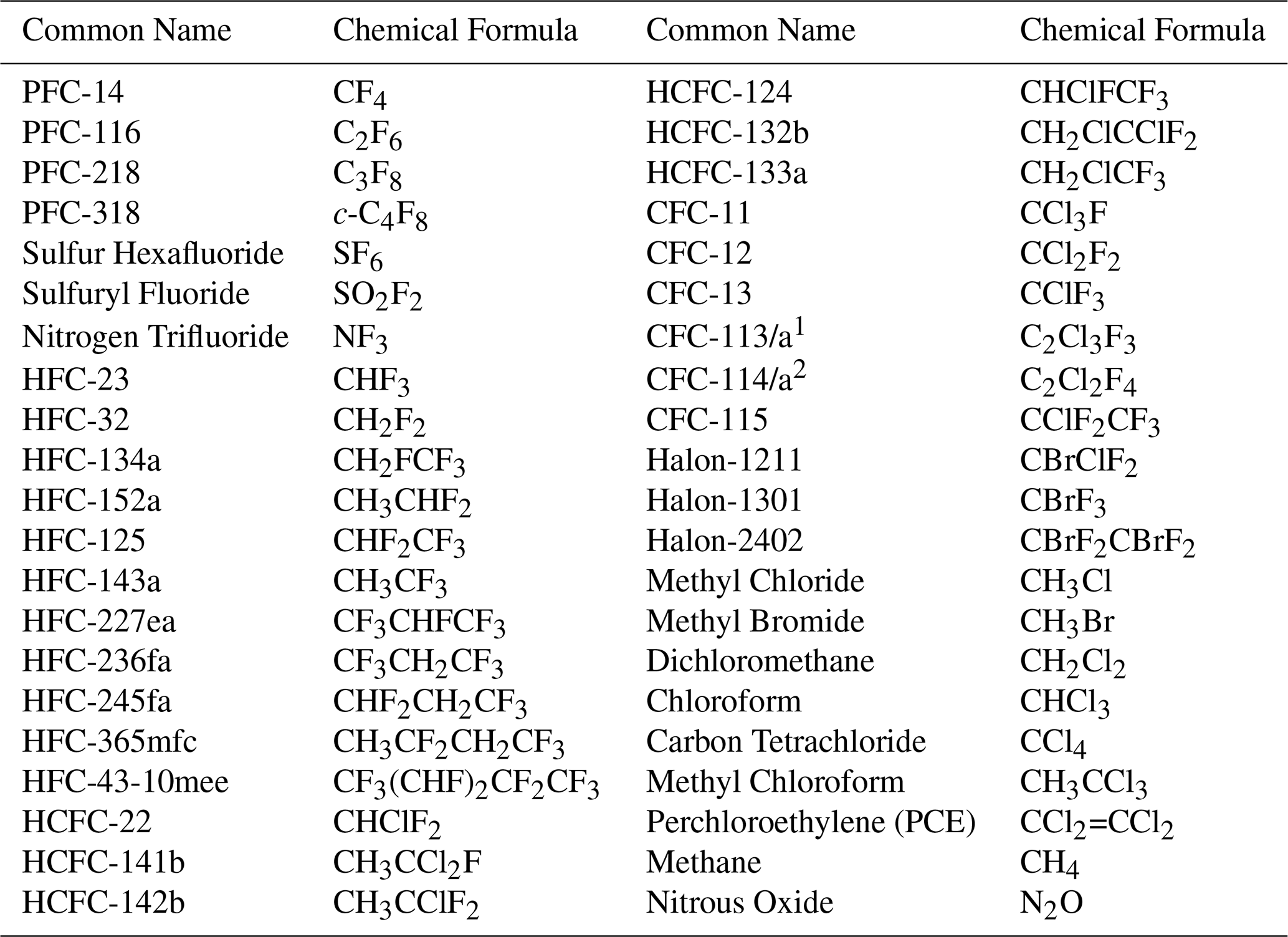
¹ CFC-113/a is a composite of the isomers CFC-113 (CClF₂CCl₂F) and CFC-113a (CCl₃CF₃). However, the contribution of each isomer to the total mole fraction is not yet well understood. ² CFC-114/a is a composite of the isomers CFC-114 (CClF₂CClF₂) and CFC-114a (CCl₂FCF₃). As footnote¹.

Global emissions and mole fraction trends are derived using AGAGE measurements coupled with a two-dimensional 12-box model of the atmosphere (Cunnold et al., 1983, 1994; Rigby et al., 2013). This is in contrast to inventory methods, or bottom-up methods, using activity data and emission factors, which can quantify expected emissions. The estimated emissions presented here, also known as top-down emissions, are inferred from measured mole fractions. The modelled global and semihemispheric mole fractions presented (see Sect. 5) are also inferred using measurements. The reason for inferring the mole fractions, rather than directly using the measurements themselves, is primarily so that mole fractions can be inferred during times where no measurements are available, e.g., due to instrument downtime.

AGAGE-derived products of ozone-depleting substances (ODSs) and greenhouse gases (GHGs) have been used in the Scientific Assessments of Ozone Depletion of the World Meteorological Organisation (WMO) (e.g., Ehhalt and Fraser, 1988; Laube and Tegtmeier, 2023; Liang and Rigby, 2023; Daniel and Reimann, 2023) and in the Assessment Reports of the Intergovernmental Panel on Climate Change (e.g., IPCC et al., 1990; Gulev and Thorne, 2023). Emission estimates using AGAGE measurements have been published in many research articles. Some recent notable outputs are the identification of excess CFC-11 emissions in eastern China after its global production phaseout (Montzka et al., 2021; Rigby et al., 2019; Park et al., 2021), of discrepancies in reported abatement and estimated global and Chinese HFC-23 emissions (Stanley et al., 2020; Adam et al., 2024), of a rapid increase in unregulated global and Chinese chloroform emissions (Fang et al., 2019), and of increases in ODS emissions used as feedstock after their phase-out for dispersive uses (Lickley et al., 2021; Vollmer et al., 2018; Western et al., 2023). Emission estimates from the AGAGE network have exposed various unusual or rapidly increasing trends in ODSs (e.g., Vollmer et al., 2015c; Liang et al., 2016; Vollmer et al., 2016; Simmonds et al., 2017; Vollmer et al., 2018; An et al., 2021; Western et al., 2022; An et al., 2023) and halogenated GHGs (Mühle et al., 2009; Miller et al., 2010; Mühle et al., 2010; Rigby et al., 2010; Vollmer et al., 2011; Arnold et al., 2014; Lunt et al., 2015; O'Doherty et al., 2014; Simmonds et al., 2016; Fortems‐Cheiney et al., 2015; Simmonds et al., 2018, 2020; Mühle et al., 2022). AGAGE measurements have also been used to identify several compounds in the atmosphere for the first time and to quantify their associated emissions (e.g., Weiss et al., 2008; Mühle et al., 2009; Schoenenberger et al., 2015; Vollmer et al., 2015a, b, 2019, 2021).

We describe the AGAGE measurements used to derive the derived products in Sect. 2, the AGAGE 12-box model in Sect. 3, and the inverse framework in Sect. 4. A brief description of the contents of the AGAGE derived products is provided in Sect. 5. The atmospheric budgets derived from the products through 2023 are then presented in Sect. 6. Finally, limitations are outlined in Sect. 7 and a brief summary is given in Sect. 9.

2 Measurements

The AGAGE network and its two predecessors have been measuring the atmospheric abundance of trace gases since 1978 (Atmospheric Lifetime Experiment, ALE: 1978–1981; Global Atmospheric Gases Experiment, GAGE: 1982–1992; AGAGE: since 1993). A complete description of the measurements made by the AGAGE network and its two predecessors is given by Prinn et al. (1983b), Prinn et al. (2000) and Prinn et al. (2018), including detailed descriptions of the measurement instruments and the calibration scales used for each trace gas. Here, we only summarise those measurements used as inputs to the 12-box model (Sect. 3), which are only from a subset of measurement sites, compounds and measurements made in the current network and its predecessors, with a focus on sites that frequently measure well-mixed background air throughout the year, that is, excluding sites that regularly measure highly polluted air masses.

The data sets described in Sect. 5 use measurements from five historic AGAGE stations and two newer AGAGE sites: Zeppelin (ZEP), Svalbard, Norway (78.9° N, 11.9° E; began 2001), Mace Head (MHD), Ireland (53.3° N, 9.9° W; began 1987), Jungfraujoch (JFJ), Switzerland (46.5° N, 8.0° E; began 2000), Trinidad Head (THD), California, USA (41.1° N, 124.2° W; began continuously in 1995), Ragged Point (RPB), Barbados (13.2° N, 59.4° W; began 1978), Cape Matatula (SMO), American Samoa (14.2° S, 170.6° W; began 1978), and at Kennaook/Cape Grim (CGO), Tasmania, Australia (40.7° S, 144.7° E; began continuously in 1978). Figure 1 shows the location of these stations. The AGAGE network contains many more sites than the ones used here. The measurement sites have been selected due to their usefulness in measuring air that is less impacted by nearby pollution, and therefore more representative of background conditions, and their longevity of measurements.

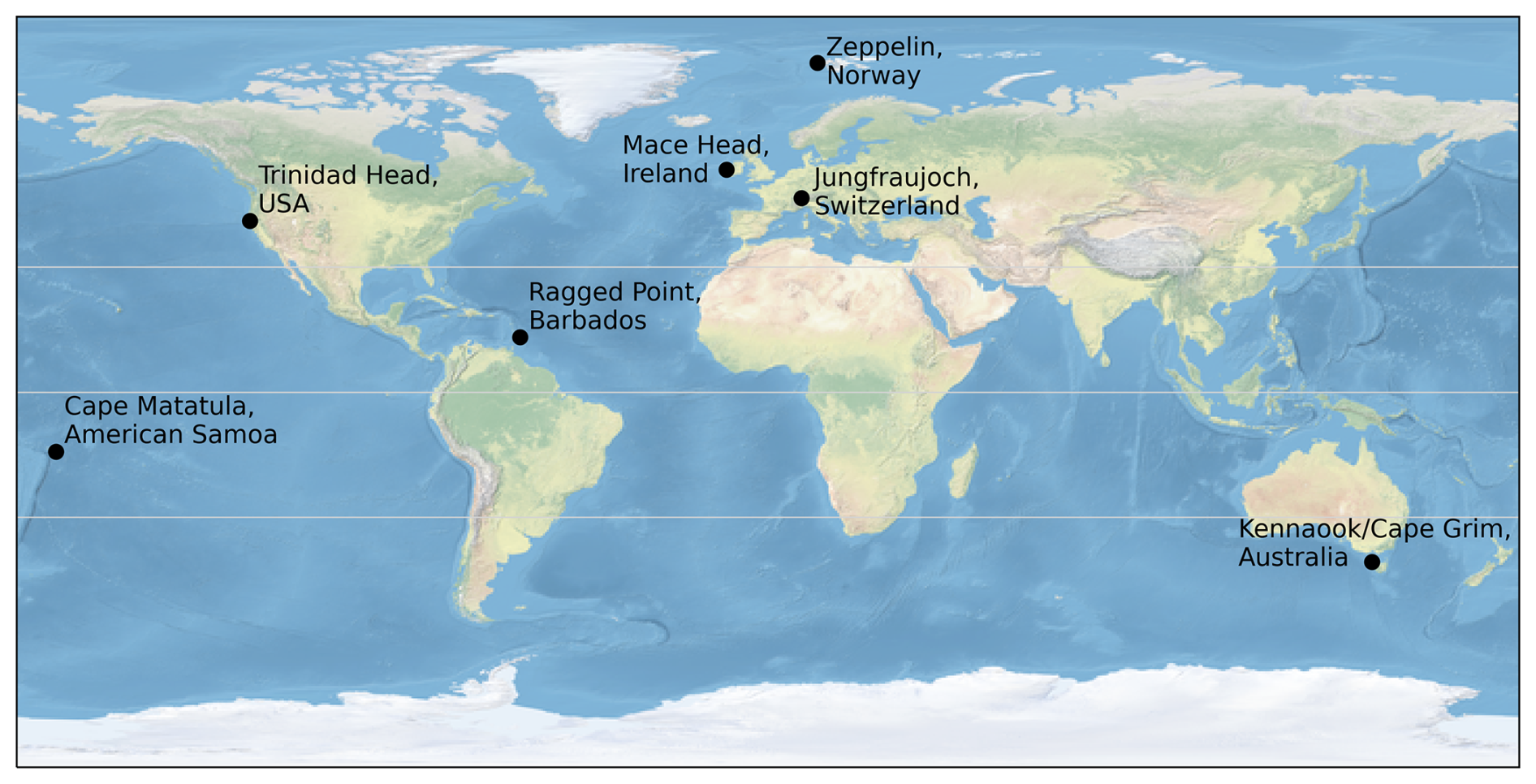
Figure 1 Locations of the AGAGE stations, from which measurements of dry-air mole fraction are currently used to derive the data sets using the 12-box model and an inverse method. Thin grey lines show the equator and ±30° N.

The data sets presented here are primarily derived from in situ high-frequency measurements (Sect. 2.1). For a subset of substances, the in situ measurements are complemented by measurements of archived air samples (Sect. 2.2). Measurements from the ALE network from two sites – Adrigole (ADR), Ireland (52° N, 10° W) and Cape Meares (CMO), Oregon (45° N, 124° W) – are used for CFC-11, CFC-12, CFC-113/a, CCl₄ and CH₃CCl₃ before measurements from MHD and THD are available. See Prinn et al. (1983b) for more information. Some publications have also used measurements of firn air, collected in Greenland and Antarctica, to derive emissions with the 12-box model (e.g., Trudinger et al., 2016; Vollmer et al., 2016, 2018), but the routinely published data sets presented here currently do not contain measurements made from firn air.

2.1 High-frequency measurements

Here, we describe the measurements used to derive global emissions and mole fraction trends. AGAGE in situ measurements of ODSs and GHGs have historically been made using multiple measurement instruments at each site. Measurements from Medusa gas chromatography mass spectrometry (GC-MS) systems (Miller et al., 2008; Arnold et al., 2012), deployed at each AGAGE site in the early to late 2000s and 2010s, are used to derive global emissions and mole fraction trends for most of the compounds listed in Table 1. Exceptions are CFC-11, CFC-12, CCl₄, and N₂O, for which measurements by the AGAGE gas chromatography `multidetector' (GC-MD) systems at MHD, THD, RPB, SMO and CGO are preferentially used (in the case of N₂O exclusively) due to higher measurement frequency and longer measurement records (see Prinn et al., 2000). These compounds are measured using electron capture detection (ECD) (Prinn et al., 2000). Sites that do not have a GC-MD instrument (JFJ and ZEP) were not used to estimate CFC-11, CCl₄, and N₂O mole fractions and emissions.

Prior to Medusa GC-MS measurements, some compounds had been measured on GC-MS adsorption–desorption systems (ADS), starting out with a prototype-ADS system at MHD in mid-1994, followed by ADS systems at MHD and CGO in late 1997 (see Simmonds et al., 1995; Prinn et al., 2000, for more information). GC-MS-ADS measurements also commenced at JFJ in 2000 (Reimann et al., 2004, 2008) and at ZEP in 2001 (Platt et al., 2022). Information about the compounds and time periods for which these GC-MS-ADS data are used to derive trends in emissions and mole fractions is contained in Prinn et al. (2025). All GC-MD, ADS, and Medusa measurements are reported on the calibration scales used by AGAGE, as detailed in Prinn et al. (2025).

Methane has been historically measured by AGAGE GC-MD systems (and its GAGE predecessor) using flame-ionization detection (FID), reported on the Tohuko 1987 scale maintained at SIO, but at some sites in recent years GC-MD CH₄ measurements have been replaced/superseded by cavity ring-down spectrometer (CRDS) instruments (Picarro) (see Prinn et al., 2018), reported on the NOAA-2004A scale (Dlugokencky et al., 2005). Extensive NOAA-AGAGE intercomparisons as well as AGAGE on-site instrument comparisons during instrument overlap have shown that the scale differences are negligible (NOAA/AGAGE ratio of 1.0001 ± 0.0007, Prinn et al., 2018). Sites that do not have a GC-MD instrument (JFJ and ZEP) were not used for methane (even when CRDS measurements were available).

The typical repeatability of the measurements made by the GC-MS Medusa and GC-MD systems discussed here range from 0.05 % for N₂O, 0.1 % for CF₄ and CFC-12, 0.3 %–1 % for most compounds, and up to 7 % for HFC-236fa of the measured standard value. For CH₄, GC-MDs achieve 0.2% and CRDS systems achieve 0.02 % (for more information see Prinn et al., 2018). The measurement repeatability is mainly compound and detector-dependent and is largely dominated by the atmospheric abundance of the compound but can also be negatively affected by site specific problems such as lab air contamination, lab temperature problems, trap temperature fluctuations, or MS filament problems.

The measurement data sets available from Prinn et al. (2025) provide details on the instruments used to measure each compound listed in Table 1, and for which period. The measurements are used in conjunction with the statistical AGAGE pollution algorithm to determine pollution free monthly mean baseline mole fractions, which are then used as input for the model and inversion to produce the data sets presented here. This method allows for the determination of monthly mean baseline mole fractions, as detailed in Sect. 2.3.

2.2 Archived air measurements

For several compounds, measurements of archived air samples are used to extend the in situ measurement record back into the past (available from Mühle et al., 2025). For the Southern Hemisphere, air collection and archiving began in 1978 with the Cape Grim Air Archive (CGAA), where air samples were taken at CGO during clean air conditions with cryogenic methods and stored in stainless steel tanks (Fraser et al., 1991; Langenfelds et al., 1996), with the intention of reconstructing the historical composition of ambient air once suitable analytical instruments and calibration scales were developed. Early measurements of the CGAA were performed on various instruments (summarized in Fraser et al., 2018), but here we focus on Medusa GC-MS measurement made in 2007 (e.g., Miller et al., 2010) and 2011 (e.g., Ivy et al., 2012), which were used in many subsequent studies (e.g., Mühle et al., 2009; O'Doherty et al., 2009; Rigby et al., 2010; O'Doherty et al., 2014). Later CGAA measurement made in 2016 (Vollmer et al., 2016) are currently not used here. These Medusa GC-MS measurements were mostly performed at the CSIRO Aspendale laboratory in Australia, but also at the Scripps Institution of Oceanography (SIO), in La Jolla, California USA. The frequency of available CGAA air samples differs, with one or two samples per year typically available before 1994, and up to nine samples available per year between 1994–1999, after which measurements of ongoing archived air samples are no longer used in this work. There is good agreement between the measurements at SIO and CSIRO of identical air samples and air samples with the same or similar fill dates.

To complement the CGAA, archived air samples from the Northern Hemisphere were gathered from several laboratories and mostly measured on Medusa GC-MS systems at SIO. Many of these tanks had been filled at THD or SIO, some at other northern hemispheric locations in the USA (such as Cape Meares in Oregon, Point Barrow in Alaska, and Niwot Ridge in Colorado) between 1973 and 2016 (Mühle et al., 2010, 2009). Unlike the CGAA, many of these samples were not originally intended for future atmospheric archive measurements and required more stringent quality control. For inert and/or volatile or very abundant compounds (such as CF₄, SF₆, NF₃, many HFCs and HCFCs) the resulting measurements were well-suited to reconstruct historic northern hemispheric abundances. Measurements of other compounds (e.g., several minor CFCs, H-2402, HCFC-22, HCFC-124, HFC-43-10mee, PFC-218) produced some anomalous data points during data processing, which resulted in less certain northern hemispheric historic abundances for these compounds. Some archived air samples from the Northern Hemisphere were also measured at CSIRO (Arnold et al., 2012; Ivy et al., 2012; Mühle et al., 2010, 2009), again generally confirming that measurements from the instruments at SIO and CSIRO can be combined.

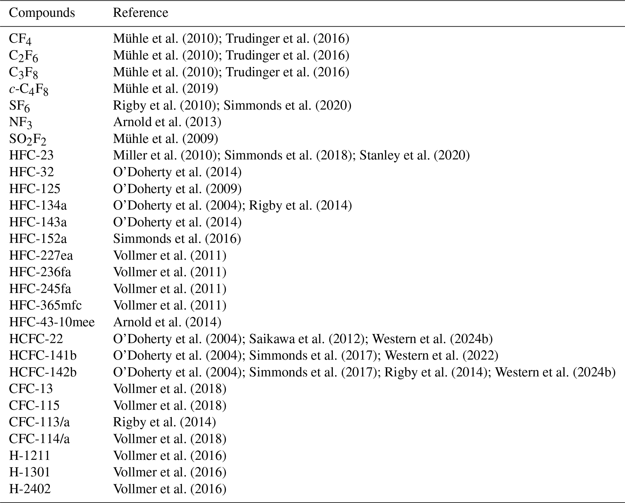
Table 2 shows the compounds that use archived air measurements in their emissions estimates. The references in Table 2 are the first publications in which archived air was used to derive emissions, and subsequent relevant publications.

Mühle et al. (2010); Trudinger et al. (2016)Mühle et al. (2010); Trudinger et al. (2016)Mühle et al. (2010); Trudinger et al. (2016)Mühle et al. (2019)Rigby et al. (2010); Simmonds et al. (2020)Arnold et al. (2013)Mühle et al. (2009)Miller et al. (2010); Simmonds et al. (2018); Stanley et al. (2020)O'Doherty et al. (2014)O'Doherty et al. (2009)O'Doherty et al. (2004); Rigby et al. (2014)O'Doherty et al. (2014)Simmonds et al. (2016)Vollmer et al. (2011)Vollmer et al. (2011)Vollmer et al. (2011)Vollmer et al. (2011)Arnold et al. (2014)O'Doherty et al. (2004); Saikawa et al. (2012); Western et al. (2024b)O'Doherty et al. (2004); Simmonds et al. (2017); Western et al. (2022)O'Doherty et al. (2004); Simmonds et al. (2017); Rigby et al. (2014); Western et al. (2024b)Vollmer et al. (2018)Vollmer et al. (2018)Rigby et al. (2014)Vollmer et al. (2018)Vollmer et al. (2016)Vollmer et al. (2016)Vollmer et al. (2016)

Table 2 Relevant publications of compounds that have used archived air measurements, alongside high frequency measurements made by AGAGE, to quantify emissions estimates.

2.3 Derivation of baseline mole fractions

Derived global emissions and mole fraction trends are inferred from monthly mean “baseline” mole fractions for each measurement site in Sect. 2. A baseline measurement is when the sampled air is well mixed within the air parcel and is not influenced by nearby pollution sources. These monthly mean baseline mole fractions are fed into the inversion framework described in Sect. 4.

Here, monthly mean baseline measurements are derived using a statistical algorithm (O'Doherty et al., 2001). The algorithm identifies measurements that are considered as baseline by taking the following steps.

1. For a given day, fit a second-order polynomial to the daily minima of measurements over a 121 d window centred on that day (i.e. using 60 d before and after). Subtract the fitted polynomial from all measurements within the window, to detrend the measurements, and calculate the median of these detrended data. Calculate the root mean square error (RMSE) using only the detrended values that fall below this median value. Classify measurements on the given day as baseline if they are within three times the RMSE of the median. Compute this step as a moving window across all days.

2. Repeat step 1 using the resultant tentative baseline measurements, with initial pollution events removed, from the first iteration of Step 1. Additionally, during this step, label measurements that fall within two to three times the new RMSE as “possibly polluted” measurements.

3. Remove the “possibly polluted” measurements if the following or preceding measurement is also labelled as a polluted measurement (i.e., greater than three times the RMSE) following Step 2.

4. The mean of the remaining baseline measurements for each calendar month is taken as the monthly mean baseline for a given measurement site.

3 AGAGE 12-box model

AGAGE measurements are combined with a 12-box model and an inverse method to produce the derived products presented here. The AGAGE 12-box model is a two-dimensional model that simulates transport of long-lived trace species in the zonal mean atmosphere (i.e., with no longitudinal component). Each trace gas is assumed to be uniformly mixed within each box. The current AGAGE 12-box model has evolved from the 9-box model originally described in Cunnold et al. (1983), which was later expanded to 12 boxes (Cunnold et al., 1994). Several subsequent publications have recoded this original model (Rigby et al., 2013), updated transport parameters or losses (e.g., Rigby et al., 2008), or developed a model adjoint (Thompson et al., 2018). The 12-box model is divided into latitudinal semi-hemispheres at the equator and 30° N and 30° S, and vertically at 500 and 200 hPa (with the surface at 1000 hPa), approximating boxes bounded at the planetary boundary layer and tropopause. See Fig. 2 for a schematic representation. The air masses of the four boxes are equal at each vertical level. The 12-box model is governed by source, transport and loss processes, which are described in the remainder of this section.

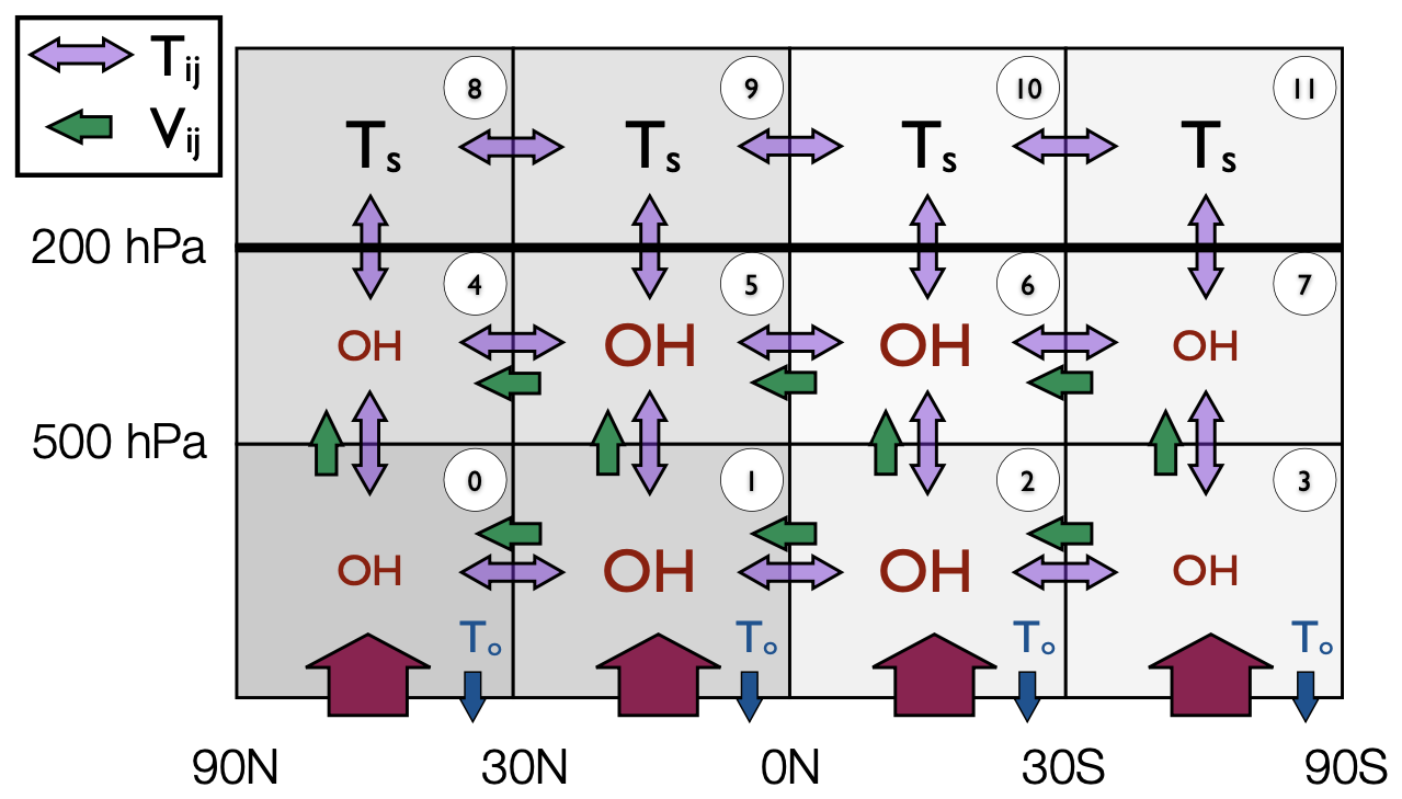
Figure 2 A schematic of the 12-box model taken from Rigby et al. (2013). The purple two-headed arrows between boxes indicate the eddy diffusion timescales and the green arrows the advection rates, which are shown in Table 3. The red arrows represent emissions into the model. Blue arrows, labelled with T_o, represent loss processes due to ocean and soil uptake. Boxes labelled with OH show where troposphoric loss due to reaction with the hydroxyl radical occurs. Boxes labelled T_s show where stratospheric loss occurs. The indices used to label each box are shown in the white circles. For methane, there is an additional loss field for the chlorine radical. For some species, such as halons, a first order loss is also assumed in the tropospheric boxes, parameterising tropospheric photolysis.

3.1 Transport

Dynamic transport in the 12-box model is represented through a parameterisation of advection and diffusion between the boxes. The change in the mass mixing ratio in surface boxes ($j=\mathrm{0},\mathrm{1},\mathrm{2},\mathrm{3}$), χ_j, over time is given by the equation

$$\begin{array}{}\text{(1)}& \begin{array}{rl}{\displaystyle \frac{\mathrm{d}{\mathit{\chi }}_j}{\mathrm{d}t}}& =-{\mathrm{1}}_{j>\mathrm{0}}\left(j\right)\left(V_{j-\mathrm{1},j}{\stackrel{\mathrm{‾}}{\mathit{\chi }}}_{j-\mathrm{1},j}+{\displaystyle \frac{(\mathrm{\Delta }\mathit{\chi }{)}_{j,j-\mathrm{1}}}{t_{j,j-\mathrm{1}}}}\right)\\ & -{\mathrm{1}}_{j<\mathrm{3}}\left(j\right)\left(V_{j+\mathrm{1},j}{\stackrel{\mathrm{‾}}{\mathit{\chi }}}_{j+\mathrm{1},j}+{\displaystyle \frac{(\mathrm{\Delta }\mathit{\chi }{)}_{j,j+\mathrm{1}}}{t_{j,j+\mathrm{1}}}}\right)\\ & -\left(V_{j+\mathrm{4},j}{\stackrel{\mathrm{‾}}{\mathit{\chi }}}_{j+\mathrm{4},j}+{\displaystyle \frac{(\mathrm{\Delta }\mathit{\chi }{)}_{j,j+\mathrm{4}}}{t_{j,j+\mathrm{4}}}}\right)-L_j+{\displaystyle \frac{E_j}{M_j}},\end{array}\end{array}$$

where V_i,k is an inverse time constant representing the mean meridional transport between boxes i and k, $t_{i,k}^{-\mathrm{1}}$ is the rate of eddy diffusion, E_j is the emissions into box j, the losses are defined collectively by L_j, and M_j is the total mass of air in box j. Other mathematical descriptors are

$$\begin{array}{}\text{(2)}& {\displaystyle }{\stackrel{\mathrm{‾}}{\mathit{\chi }}}_{i,k}={\displaystyle \frac{\mathrm{1}}{\mathrm{2}}}({\mathit{\chi }}_i+{\mathit{\chi }}_k),\text{(3)}& {\displaystyle }(\mathrm{\Delta }\mathit{\chi }{)}_{i,k}={\mathit{\chi }}_i-{\mathit{\chi }}_k,\end{array}$$

and the indicator function, which is defined where

$$\begin{array}{}\text{(4)}& {\mathrm{1}}_A\left(j\right)=\left\{\begin{array}{ll}\mathrm{1}& \text{if }A\text{is true}\\ \mathrm{0}& \text{otherwise}.\end{array}\right.\end{array}$$

For tropospheric boxes ($j=\mathrm{4},\mathrm{5},\mathrm{6},\mathrm{7}$), the mass mixing ratio is given by

$$\begin{array}{}\text{(5)}& \begin{array}{rl}{\displaystyle \frac{\mathrm{d}{\mathit{\chi }}_j}{\mathrm{d}t}}& =-{\mathrm{1}}_{j>\mathrm{4}}\left(j\right)\left({\displaystyle \frac{\mathrm{5}}{\mathrm{3}}}{V}_{j-\mathrm{1},j}{\stackrel{\mathrm{‾}}{\mathit{\chi }}}_{j-\mathrm{1},j}+{\displaystyle \frac{(\mathrm{\Delta }\mathit{\chi }{)}_{j,j-\mathrm{1}}}{t_{j,j-\mathrm{1}}}}\right)\\ & -{\mathrm{1}}_{j<\mathrm{7}}\left(j\right)\left({\displaystyle \frac{\mathrm{5}}{\mathrm{3}}}{V}_{j+\mathrm{1},j}{\stackrel{\mathrm{‾}}{\mathit{\chi }}}_{j+\mathrm{1},j}+{\displaystyle \frac{(\mathrm{\Delta }\mathit{\chi }{)}_{j,j+\mathrm{1}}}{t_{j,j+\mathrm{1}}}}\right)\\ & -\left({\displaystyle \frac{\mathrm{5}}{\mathrm{3}}}{V}_{j-\mathrm{4},j}{\stackrel{\mathrm{‾}}{\mathit{\chi }}}_{j-\mathrm{4},j}+{\displaystyle \frac{\mathrm{5}}{\mathrm{3}}}{\displaystyle \frac{(\mathrm{\Delta }\mathit{\chi }{)}_{j,j-\mathrm{4}}}{t_{j,j-\mathrm{4}}}}\right)\\ & -{\displaystyle \frac{(\mathrm{\Delta }\mathit{\chi }{)}_{j,j+\mathrm{4}}}{t_{j,j+\mathrm{4}}}}-L_j,\end{array}\end{array}$$

and finally for the stratospheric boxes ($j=\mathrm{8},\mathrm{9},\mathrm{10},\mathrm{11}$),

$$\begin{array}{}\text{(6)}& \begin{array}{rl}{\displaystyle \frac{\mathrm{d}{\mathit{\chi }}_j}{\mathrm{d}t}}& =-{\mathrm{1}}_{j>\mathrm{8}}\left(j\right){\displaystyle \frac{(\mathrm{\Delta }\mathit{\chi }{)}_{j,j-\mathrm{1}}}{t_{j,j-\mathrm{1}}}}-{\mathrm{1}}_{j<\mathrm{11}}\left(j\right){\displaystyle \frac{(\mathrm{\Delta }\mathit{\chi }{)}_{j,j+\mathrm{1}}}{t_{j,j+\mathrm{1}}}}\\ & -{\displaystyle \frac{\mathrm{3}}{\mathrm{2}}}{\displaystyle \frac{(\mathrm{\Delta }\mathit{\chi }{)}_{j,j-\mathrm{4}}}{t_{j,j-\mathrm{4}}}}-L_j.\end{array}\end{array}$$

Equations (1), (5) and (6) are solved using a Runge-Kutta (RK4) method (see e.g. Butcher, 1996) with a time step of 48 h.

3.1.1 Transport coefficients

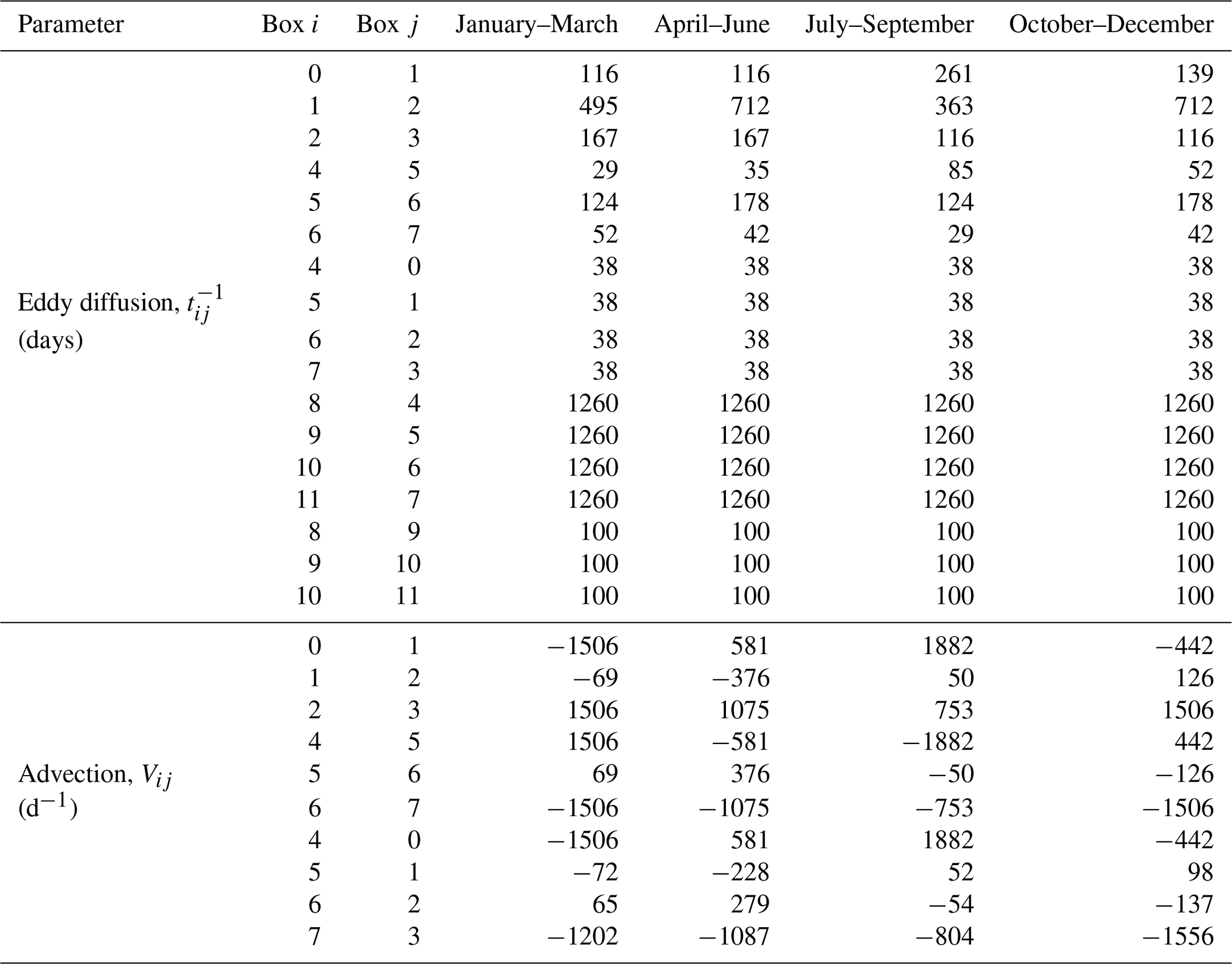
The mean meridional transport and eddy diffusion rates between the boxes vary seasonally but repeat annually. The advection parameters are taken from Cunnold et al. (1994), which were derived from a study by Newell et al. (1969). The original eddy diffusion terms estimated by Cunnold et al. (1983) have been adjusted in various ways in different studies. For example, Rigby et al. (2013) optimised the parameters simultaneously with CFC-11, CFC-12, and CFC-113 and CH₃CCl₃ lifetimes using AGAGE observations of those species, and Rigby et al. (2008) attempted to account for some inter-annual variability in transport by scaling inter-hemispheric exchange rates as a function of climate indices such as the Southern Oscillation Index. Here, we use the parameterisation that has been used in recent studies (e.g., Laube and Tegtmeier, 2023; Liang and Rigby, 2023) in which interannually repeating eddy diffusion parameters were derived based on simulations of an inert tracer in the MOZART three-dimensional model (Emmons et al., 2010). MOZART was run using NCEP/NCAR reanalyses for SF₆ for the years 2007–2009, as described in Rigby et al. (2011b). The box model mole fractions were compared to zonal mean mole fractions output from MOZART averaged over regions of the atmosphere chosen to be approximately representative of the mass-weighted centre of each box (45–80° for the extratropical boxes and 10–20° in the tropical boxes, and 1000–700, 400–300, and 100–50 hPa in the vertical). These seasonal advection and eddy diffusion parameters are summarised in Table 3. The temperature in each box, which is used to calculate OH losses, is applied monthly, but is inter-annually repeating and is taken from the 1990–2010 mean from the NCEP/NCAR reanalysis (Kalnay et al., 1996).

Table 3 Transport parameters between boxes. Eddy diffusion parameters are available for transport between all boxes. Advection does not occur in the stratospheric boxes. Advection timescales are mass conserving.

3.2 Sinks and loss processes

The 12-box model has various loss processes, depending on the compound and box, which are summarised in Table 4. Where target lifetimes in the literature are given as a range, the median (with respect to the inverse lifetime, or loss frequency) is used. Compounds with total atmospheric lifetimes greater than 10 000 years are considered to have no atmospheric sink.

Table 4 The loss coefficients for losses due to reaction with OH and the target lifetimes for loss process in the stratosphere, due to soil/ocean uptake and tropospheric losses other than OH. Losses due to OH are taken from Burkholder et al. (2020) and target lifetimes are taken from Burkholder and Hodnebrog (2023), where available. The stratospheric lifetime of methane is taken from Myhre et al. (2014). OH_A is the Arrhenius factor and OH${}_{E/R}$ is the molar activation energy. Citations for these values are provided in the text.

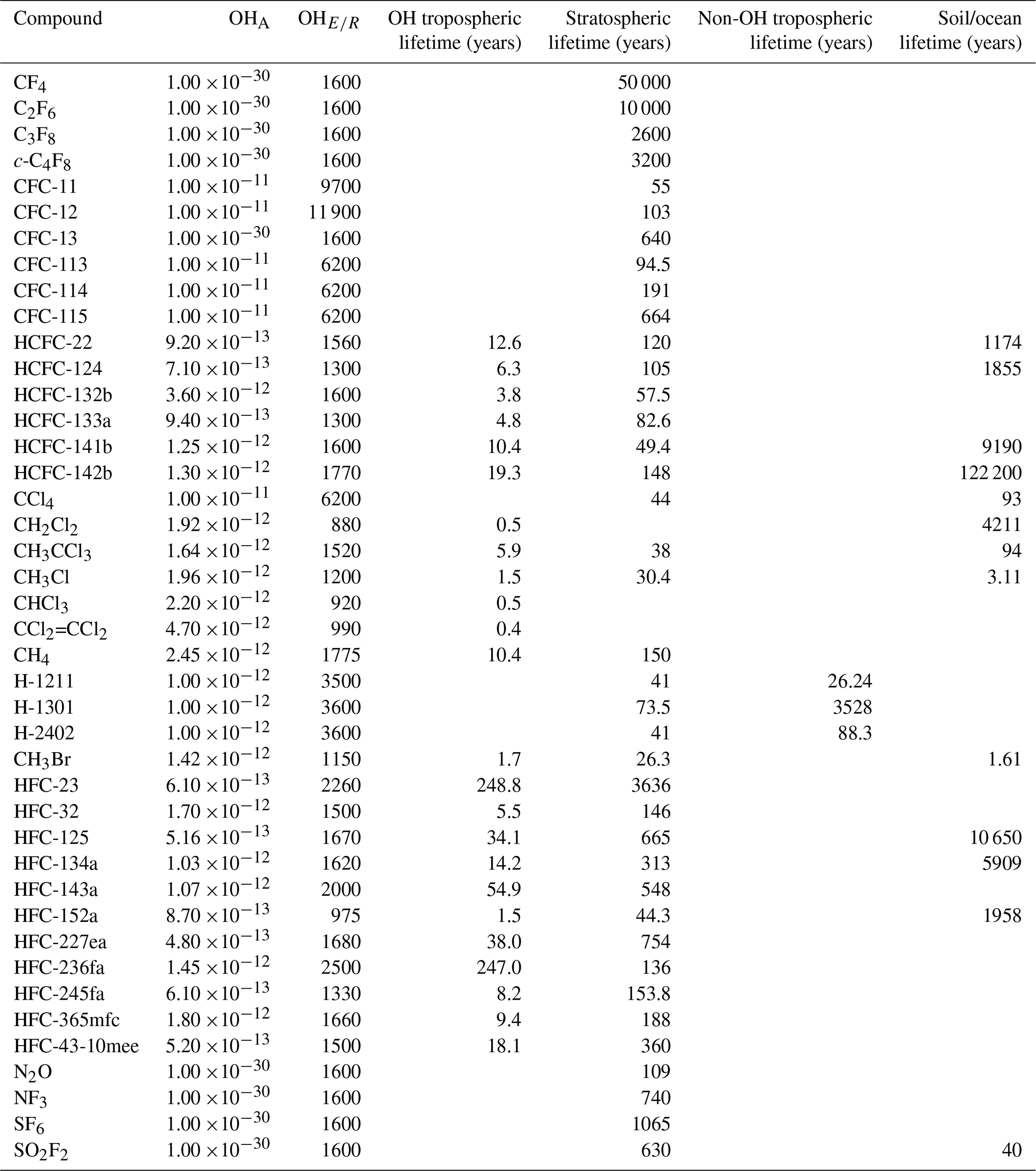
Losses due to the reaction with the hydroxyl radical (OH), for compounds with non-negligible OH losses, are calculated in the tropospheric boxes (boxes 0–7, see Fig. 2). The concentrations of OH (taken from Spivakovsky et al., 2000) are seasonally varying but annually repeating and the OH field is adjusted so that the model mole fraction simulation of CH₃CCl₃, whose loss is dominated by OH, is consistent with AGAGE observations (using an approach similar to Rigby et al., 2013, but for inter-annually repeating, rather than inter-annually varying OH). All compounds are passive with respect to the OH loss, meaning that there is no loss of OH due to the sink process. Losses due to OH are computed using a first-order rate constant, using the Arrhenius equation and the temperature fields from Sect. 3.1.1. The Arrhenius factor and molar activation energy for each compound are taken from Burkholder et al. (2020). Where the OH sink is thought to be negligible and is not reported, a default Arrhenius factor of 1 $\times {\mathrm{10}}^{-\mathrm{30}}$ and $E/R$ factor of 1600 is assumed.

Losses in the stratosphere (boxes 8–11 in Fig. 2), due to reaction with excited atomic oxygen, stratospheric OH and photolysis are calculated using a single first-order loss frequency that accounts for the overall loss due to these processes. Lyman-α photolysis is treated as a loss in the stratospheric boxes in the model, even though this sink is a mesospheric loss process. A suitable first-order rate constant for stratospheric losses for each compound is found by optimisation, such that the steady-state stratospheric lifetime equals that in Burkholder and Hodnebrog (2023). An exception is the stratospheric lifetime of methane, which is taken from Myhre et al. (2014). Initial stratospheric losses are distributed latitudinally and temporally following Golombek and Prinn (1986), and these values are adjusted by a single factor in the optimisation, such that the relative temporal and spatial gradients are not altered. Target stratospheric steady state lifetimes are summarised in Table 4.

Compounds with sink processes due to ocean and/or soil uptake have losses in the lowest layer boxes (0–3 in Fig. 2). In a similar manner to the stratospheric losses, ocean and soil losses are treated together as a single loss process. These losses are computed as a first-order loss, where the first order rate constant is optimised to give the steady-state target lifetime of the total soil and ocean loss (Burkholder et al., 2020; Yvon-Lewis and Butler, 2002).

For methane, loss from reaction with the chlorine radical is included in the model. The chlorine distribution is taken from Sherwen et al. (2016). First order rate constants are calculated using the Arrhenius equation (Burkholder and Hodnebrog, 2023).

Tropospheric loss processes so far not addressed are present for some compounds, such as a non-negligible photolysis sink in the troposphere. These other tropospheric sinks are implemented in boxes 4–7 (Fig. 2) using a first-order rate constant that is optimised in a similar way to that of the stratospheric and ocean/soil sinks, using a target tropospheric lifetime (Burkholder and Hodnebrog, 2023), considering the other loss processes present. The spatial and temporal gradient of this loss follows that of loss from tropospheric OH.

4 Inverse method

The emission and global mole fraction trends for the compounds listed in Table 1 are derived using an inverse modelling framework. The approach relies on the measurements described in Sect. 2, and a priori emissions estimates, to inform an estimate of emissions and mole fraction trends using Bayesian inference (Sect. 4.2). This section describes the statistical framework to derive these estimates, the treatment of errors and uncertainties, and the a priori emissions used.

4.1 Statistical framework

The inverse framework here generally follows that of Rigby et al. (2011a, 2014). Emissions are derived based on the comparison of simulated mole fractions in the surface boxes and monthly background mean AGAGE observations. The monthly mean mole fraction in each box is calculated as the mean of the monthly mean mole fractions from all available measurement sites located in that box. We define x as the deviation (in Gg yr⁻¹) from an a priori estimate of emissions taken from available bottom-up estimates of global emissions in the literature, x_a (see Sect. 4.2). The corresponding observation y is the deviation of the measured mole fractions from the modelled mole fraction using these a priori emissions. The relationship between the difference in emissions and surface mole fraction from the a priori estimate is

$$\begin{array}{}\text{(7)}& \mathit{y}=\mathbf{H}\mathit{x}+\mathit{ϵ},\end{array}$$

where H is a sensitivity matrix relating emissions to surface mole fractions and ϵ is a stochastic error, resulting from error in the mole fraction measurements. The vector x is derived either monthly, seasonally or annually for each box, depending on the compound in question (see Table S1 in the Supplement for this information). The sensitivity matrix H is derived using the linear relationship between emissions and surface mole fractions by running the model with base (a priori) emissions and again with perturbed emissions (+1 Gg) for each surface box for each time period defined in Table S1. The sensitivity of the mole fraction to emissions is calculated until the end of the period where measurements are available. The surface mole fractions (deviation), y, are baseline monthly means as detailed in Sect. 2.3.

An initial first guess at the initial conditions of the mole fraction in the 12 boxes of the model uses a nine-year spin-up period using the a priori emissions field. The initial conditions (and H) are recursively adjusted to approximate the measurements using the a priori emissions. Sensitivities (and derived emissions) begin three years before the earliest measurement. These initial three years account for model spin-up and are not included in the output data sets.

Under the Bayesian framework, we choose to place a prior constraint on the growth in emissions, rather than their absolute value (Rigby et al., 2011a). The growth matrix D operates on the emissions x, to produce an emissions growth value, which we constrain by the a priori emissions growth g. The uncertainty in the a priori emissions growth is taken as a percentage of the maximum a priori emissions, and the percentages used are defined in Table S1 for each compound, where no box will have a growth less than 1 % of the maximum global growth. Uncertainty in this growth is assumed to be independent between boxes and time steps, which we contain in the matrix P.

We separate the random and systematic errors due to the measurements and modelling. Only the random components are included in the statistical evaluation of x and are assumed to be uncorrelated between boxes and time steps. These random errors are contained in the matrix R. The diagonal is composed of the quadratic sum of the typical measurement error (given in Table S1) and the variability of the baseline mole fractions in that month (see Sect. 2.3). This latter term is assumed to be a measure of model error, by accounting for the magnitude of variability not accounted for in the model.

Under an assumption of a normal likelihood and prior probability, the resultant relationship for the probability of the emissions given the measurements (deviation) is,

$$\begin{array}{}\text{(8)}& \begin{array}{rl}-\ln \text{P}(\mathit{x}\mid \mathit{y})& \propto (\mathit{y}-\mathbf{H}\mathit{x}{)}^T{\mathbf{R}}^{-\mathrm{1}}(\mathit{y}-\mathbf{H}\mathit{x})\\ & +(\mathbf{D}\mathbf{x}-\mathit{g}{)}^T{\mathbf{P}}^{-\mathrm{1}}(\mathbf{D}\mathbf{x}-\mathit{g}),\end{array}\end{array}$$

which, by completing the square, allows determination of the maximum a posteriori probability (MAP) estimate of emissions, $\widehat{\mathit{x}}$, using

$$\begin{array}{}\text{(9)}& \widehat{\mathit{x}}=\widehat{\mathbf{P}}({\mathbf{H}}^T{\mathbf{R}}^{-\mathrm{1}}\mathit{y}+{\mathbf{D}}^T{\mathbf{P}}^{-\mathrm{1}}\mathit{g}),\end{array}$$

where

$$\begin{array}{}\text{(10)}& \widehat{\mathbf{P}}=({\mathbf{H}}^T{\mathbf{R}}^{-\mathrm{1}}\mathbf{H}+{\mathbf{D}}^T{\mathbf{P}}^{-\mathrm{1}}\mathbf{D}{)}^{-\mathrm{1}},\end{array}$$

and $\widehat{\mathbf{P}}$ is the resultant posterior covariance matrix, representing the random error in the emissions estimate. The estimate $\widehat{\mathit{x}}$ is added to the initial a priori emissions to give the estimated total emissions. The posterior mean mole fractions are estimated using the relationship

$$\begin{array}{}\text{(11)}& \widehat{\mathit{y}}=\mathbf{H}\widehat{\mathit{x}}+\mathbf{H}{\mathit{x}}_a.\end{array}$$

Combined systematic and random uncertainties are derived through the random sampling of systematic uncertainties and the Cholesky decompostion of $\widehat{\mathbf{P}}$. The systematic uncertainties are due to errors in the calibration, lifetime and transport. Calibration uncertainty is treated as a percentage offset, where the one standard deviation calibration uncertainties for each compound are defined in Table S1. The systematic component of transport error is assumed to be 1 % of emissions for all substances (one standard deviation). Lifetime error variance is calculated as,

$$\begin{array}{}\text{(12)}& {\mathit{\sigma }}_x^{\mathrm{2}}=(B{\mathit{\sigma }}_{\frac{\mathrm{1}}{\mathit{\tau }}}{)}^{\mathrm{2}},\end{array}$$

where B is the total atmospheric burden of the compound and ${\mathit{\sigma }}_{\frac{\mathrm{1}}{\mathit{\tau }}}$ is the total inverse lifetime error (Ko et al., 2013) (see Rigby et al., 2014, for more information). The assumed lifetime uncertainty is shown in Table S1 for each compound. The total uncertainty is then taken as the standard deviation from this ensemble.

4.2 A priori emissions

An initial set of estimates of the emissions for each compound has been compiled over time. These are from a variety of sources and are included in the AGAGE-derived data sets. Given the longevity of measurements made by the AGAGE network and their widespread use, there could be a lack of independence of the a priori emissions if taken from widely used emissions scenarios, which may have been, at least partly, informed by mole fraction measurements and/or emissions derived by AGAGE (e.g., Meinshausen et al., 2020). We have therefore strived, insofar as possible, to use independent a priori emissions estimates.

A priori emissions for CF₄, C₂F₆, C₃F₈, c-C₄F₈, HFC-23, HFC-32, HFC-125, HFC-134a, HFC-143a, HFC-152a, HFC-227ea, HFC-236fa, HFC-245fa, HFC-365mfc, HFC-43-10mee, HCFC-141b, HCFC-142b and SF₆ are taken from the gridded flux maps from the Emissions Database for Global Atmospheric Research (EDGAR) v8 (Crippa et al., 2023). These are annual emissions from 1970–2022, with the exception of C₃F₈, which spans 1975–2022. HFC-23 emissions prior to 1970 are taken from Miller et al. (2010). After 2022, emissions for all compounds are repeated using the values from 2022.

The EDGAR v8 inventory also includes NF₃ but its global emissions are erroneously small compared to other literature sources (e.g., Arnold et al., 2013; Liu et al., 2024). We instead use the PRIMAP-hist v2.6 national historical emissions time series for NF₃ (Gütschow et al., 2016, 2024). Emissions are quantified until 2023 in the database and repeated thereafter.

CFC-11, CFC-12 and CFC-113/a a priori emissions are the bottom-up estimates compiled in Rigby et al. (2013), which were informed by a variety of inventory compilations and forecasts (e.g., McCulloch et al., 2001, 2003). CH₃CCl₃ was compiled in a similar manner, but emissions have been repeated after 2015 until present. A priori estimates of CFC-114/a and CFC-115 were compiled from a variety of sources (see Vollmer et al., 2018, and its supplementary information). To the best of our knowledge, no comprehensive inventory of global emissions of CFC-13 exists, so we assume that the a priori emissions for CFC-13 are a seventh of those of CFC-115 (see the supplementary information of Vollmer et al. (2018) for the rationale behind this approximation, which is based on available ratios of production of the two compounds).

The a priori emissions estimate for halons – Halon-1211, Halon-1301 and Halon-2402 – are taken from the bottom-up emissions published by Vollmer et al. (2016). These estimates were originally compiled by HTOC (2014) but the values were not made available.

The historic a priori estimates of CCl₄ emissions are based on information from industry on the production of CFCs (Archie McCulloch, personal communication, 2013). Estimates since 2010 are taken from Sherry et al. (2018). The use of carbon tetrachloride as a feedstock for the production of CFCs was its major source of emissions prior to the phase out of the production of CFCs for dispersive uses. There are continued unexplained global emissions of carbon tetrachloride, which makes a comprehensive bottom-up inventory of its emissions difficult (Liang et al., 2016; Daniel and Reimann, 2023).

Little is known about the source of emissions of HCFC-132b and HCFC-133a (Fraser et al., 2014; Vollmer et al., 2015c, 2021). These two substances are assumed a priori to have constant emissions, with an annual mean of 1 Gg yr⁻¹ with a small seasonal trend, following Vollmer et al. (2021). HCFC-22 a priori emissions are an extension of the bottom-up emissions derived by Miller et al. (1998), using the HCFC-22 production data from multiple sources (Miller et al., 2010). These emissions estimates extend through 2009, after which the emissions are assumed to remain constant. A bottom-up inventory of emissions for HCFC-124 was compiled for 1990–2001 and projected to 2015 under three scenarios (Ashford et al., 2004). We use Scenario 2, which envisaged improvements to reduce HCFC emissions over the policy at the time of compilation. Emissions are repeated after 2015.

PCE (CCl₂=CCl₂) a priori emissions are taken from Montzka and Reimann (2010), which was compiled from multiple sources (McCulloch et al., 1999; Keene et al., 1999; Simmonds et al., 2006). CH₂Cl₂, CHCl₃ and CH₃Cl estimates are based on the emission estimates compiled in Xiao (2008) and methyl bromide in Yvon-Lewis and Butler (1997). Given the lack of a priori information about emissions of these gases, they are assumed to be constant in time.

The a priori estimates for SO₂F₂ were described in Mühle et al. (2009), which were compiled using information on the production of SO₂F₂. Given the use of SO₂F₂ as a fumigant, it can be assumed that its emissions will be approximately equal to its production in a given year. Our a priori emissions estimate for this compound was constant after 2007.

Emissions for N₂O are built from various sources. Anthropogenic emissions are from EDGARv8.0 for the years 1970–2022, and the 2022 emissions are repeated thereafter (Crippa et al., 2023). Ocean emissions are from the ECCO-Darwin model for the period 2009–2013 (Resplandy et al., 2024), and annually repeating before 2009 using the 2009 emissions and after 2013 using the 2013 emissions. Other natural emissions are from Saikawa et al. (2014) for 1990–2008, with annually repeating values using emissions from 1990 and 2008 before and after these dates. This estimate is within the range of bottom-up derived N₂O net flux (Tian et al., 2024).

Anthropogenic a priori emissions of CH₄ are taken from EDGAR v8.0 (Crippa et al., 2023), wetland emissions are taken from WetCHARTS v1.3.1 (Bloom et al., 2017), biomass burning from the Global Fire Emissions Database (GFED) (van der Werf et al., 2017), freshwater emissions from Stell et al. (2021), rice from Yan et al. (2009), and other natural sources from Fung et al. (1991); Ruppel and Kessler (2017). Years without estimates from a particular source are filled with the closest year of available data. The total emissions are within the uncertainty of other well-used bottom-up total flux estimates (e.g. Saunois et al., 2025).

4.3 Derived global mole fractions and growth rates

The presented mole fractions for each semihemisphere are those of the MAP estimate of the emissions, and their uncertainty, forward simulated through the 12-box model. The global annual mole fraction is the mean of the four surface-level boxes. The growth rates of the mole fraction are derived from $\widehat{\mathit{y}}$ (see Sect. 4.1) using backward differencing. These growth rates are then smoothed using a Kolmogorov–Zurbenko (KZ) filter (Yang and Zurbenko, 2010) with a window size of 9 and a filtering degree of 4. The uncertainties for the estimated mole fractions and their growth rates are derived from the Monte Carlo ensemble described in Sect. 4.1.

5 Published products

We aim to provide updated estimates of global missions and mole fraction trends annually, with a target time delay of approximately six months following the quality control of the atmospheric measurements by the AGAGE community. The release of data sets of specific substances may be withheld if the scientific integrity of the measurement of a specific substance is under question, e.g., due to emerging chromatographic interference, or if further insights into the data are required. Recent emission estimates (within the previous ∼2 years) should be treated as preliminary as some of the underlying measurement data may not be fully vetted and/or calibration tanks may not have been returned from the measurement sites to the AGAGE central calibration laboratory for re-calibration.

For each substance, a number of derived products are provided. These summary data sets provided are as follows:

• Emissions:

  • -

    Global annual emissions (with and without systematic uncertainties)

• Mole fraction:

  • -

    Global calendar year mean surface mole fraction (mid-year centred)

  • -

    Global annual January-centred surface mole fraction

  • -

    Semihemispheric monthly mole fraction at each altitude level

  • -

    Semihemispheric monthly measured surface mole fraction

• Surface mole fraction growth rate:

  • -

    Global monthly mole fraction growth rate

  • -

    Semihemispheric monthly mole fraction growth rate.

The data sets are provided as text files with comma-separated values (csv) and are available to download from Western et al. (2025). Each data set includes both the mean posterior estimate of the emissions/mole fraction (see Sect. 4) and its 1-standard deviation uncertainty. Annual emissions are provided including either random uncertainties or combined random and systematic uncertainties (see Sect. 4.1). These two uncertainty estimates are provided to aid the calculation of uncertainty in quantities that are, or are not, influenced by systematic uncertainties. The uncertainty in an emissions change between two years is not strongly influenced by systematic uncertainties of the type estimated here, whereas the uncertainty in the absolute emissions in a particular year is. For example, if an error in the measurement calibration scale for an inert compound causes a constant absolute offset across the whole measurement record, the derived emissions would also be offset by some near-constant value, yet the growth in emissions would remain unchanged. The annual and monthly quantities are centred around the corresponding calendar year or month, unless otherwise stated.

6 AGAGE derived global budgets

Here we give a summary of the budgets of non-CO₂ GHGs and ODSs derived from the AGAGE network through 2023 using the measurements from Prinn et al. (2025) and the methodology outlined above. We present these budgets separately for the long-lived halogenated gases that are primarily of synthetic anthropogenic origin in Sect. 6.1, and CH₄ and N₂O, whose fluxes have substantial non-anthropogenic components, in Sect. 6.2. Given the uncertain natural sources, short lifetime and uncertain impacts of very short-lived chlorinated substances (CH₂Cl₂, CHCl₃ and CCl₂=CCl₂), CH₃Cl and CH₃Br, we present these separately in Sect. 6.3. Emissions, global mole fractions, and their growth rates for each individual compound can be found in the supplementary information.

6.1 Halogenated ozone-depleting substances and greenhouse gases

The annual global emissions of synthetic greenhouse gases are presented in Fig. 3. We group compounds as CFCs, HCFCs, HFCs, Halons, “other F-gases” (SF₆, NF₃ and SO₂F₂), PFCs and “Solvents” (CCl₄ and CH₃CCl₃). These emissions are shown in terms of the direct climate warming potential of the emissions over a 100 year time horizon (GWP-100, CO₂-eq) and their ozone depletion potential (ODP, CFC-11-eq) (Burkholder and Hodnebrog, 2023), respectively.

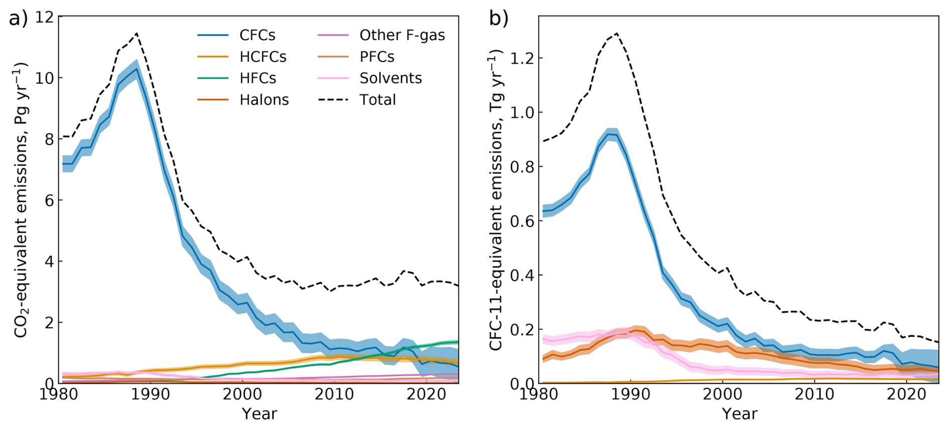
Figure 3 Emissions of synthetic greenhouse gases presented as the total, weighted in terms of their (a) global warming potential (CO₂-equivalent emissions) over a 100-year time horizon and (b) ozone-depleting potential (CFC-11-equivalent emissions). The category “solvents” contains carbon tetrachloride and methyl chloroform, and the category “other F-gases” contains SF₆, NF₃ and SO₂F₂.

The total CO₂-equivalent emissions from synthetic greenhouse gases were 3.2 ± 0.6 Pg CO₂-eq in 2023, and have remained relatively unchanged over the last 20 years of the record (Fig. 3). There has been an overall reduction in CO₂-equivalent emissions due to reduction of CFC emissions since the 1990s. This reduction has been partially offset by a growth and recent decline in emissions of HCFCs (e.g., Western et al., 2024b), and the continuing growth of HFCs and, to a lesser extent, PFCs and other F-gases. It can reasonably be expected that the emissions of synthetic greenhouse gases will decrease in the coming years given the controls on HFCs under the Kigali Amendment to the Montreal Protocol and other commitments as part of the Paris Agreement and other climate policies (Velders et al., 2022; Daniel and Reimann, 2023).

The emissions of the ozone-depleting synthetic greenhouse gases (CFCs, HCFCs, halons and chlorinated solvents) were 152 ± 66 Gg CFC-11-eq in 2023. Emissions of these ozone-depleting substances are now at their lowest since measurement-derived emission records began, despite some small, but impactful, fluctuations in total emissions, meaning that this decline has not been entirely monotonic (see, e.g., Montzka et al., 2018, 2021).

The global abundances of the synthetic greenhouse gases are shown in Fig. 4, using the same compound groupings as Fig. 3. The impact on climate is shown in terms of direct radiative forcing, which considers stratospheric adjustments to the instantaneous radiative forcing, and also tropospheric adjustments for CFC-11 and CFC-12 (Shine and Myhre, 2020; Hodnebrog et al., 2020; Burkholder and Hodnebrog, 2023). The impact on ozone depletion is shown in terms of equivalent effective chlorine (Montzka et al., 1996), which is the global mean surface chlorine mole fraction (number of chlorine atoms in a given species multiplied by its mole fraction).

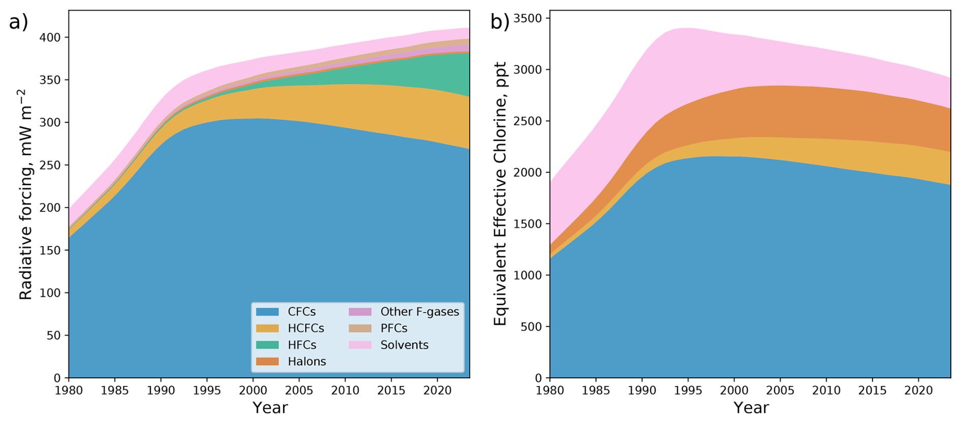
Figure 4 Global abundance of synthetic greenhouse gases in terms of (a) the direct radiative forcing and (b) equivalent tropospheric chlorine. The direct radiative forcing considers stratospheric adjustments to the instantaneous radiative forcing, and also the tropospheric adjustments for CFC-11 and CFC-12.

The direct radiative forcing of synthetic greenhouse gases has increased since measurements of their atmospheric abundance began, reaching 411 ± 5 mW m⁻² in 2023. Global abundances of CFCs, chlorinated solvents and HCFCs are now decreasing (Montzka et al., 1996; Western et al., 2024b), and are being offset by an increasing abundance of HFCs, PFCs (foremost CF₄) and other F-gases (foremost SF₆).

Conversely, the equivalent effective chlorine has declined since its peak in 1994, to 2920 ± 30 ppt in 2023. This is driven by the decreasing abundances of CFCs, halons and solvents (foremost CH₃CCl₃) in the atmosphere (Montzka et al., 1996) and also more recently by a fall in the abundance of HCFCs (Western et al., 2024b).

6.2 Methane and Nitrous Oxide

Figure 5 shows the global and semihemispheric mole fractions of methane and nitrous oxide, the growth rate of these mole fractions and the north-south inter-hemispheric difference. Figure 6 shows their global mean emissions.

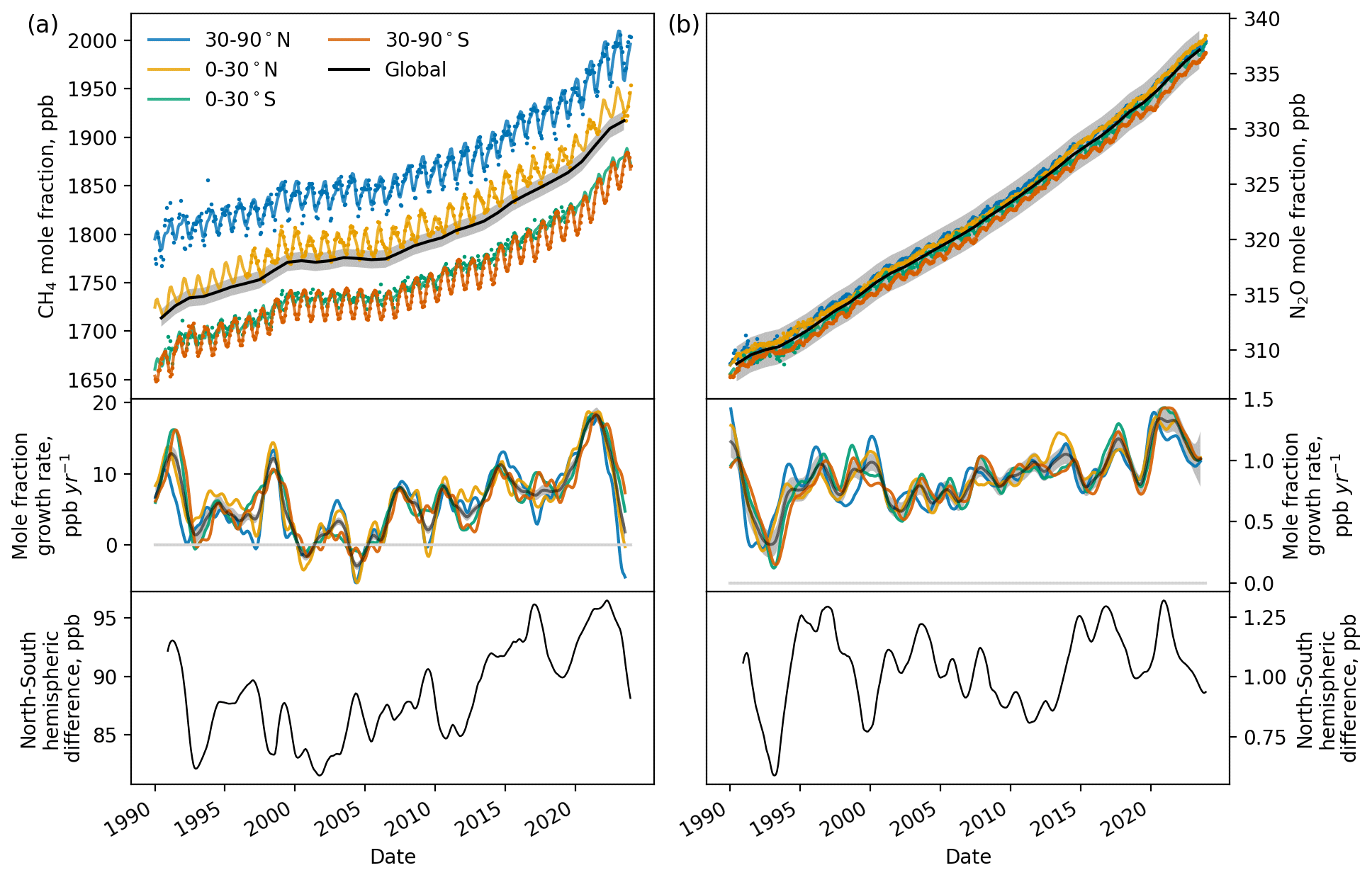
Figure 5 The global and semihemispheric mole fraction for (a) methane and (b) nitrous oxide (top panels), the growth rate in these mole fractions (middle panels) and the north-south interhemispheric difference (lower panels) for 1990–2023. Observed mole fractions are shown in the top panels by the small circles and fits to these observations are shown with lines. The black lines indicate global mean quantities with 1σ uncertainties shown by the grey shading.

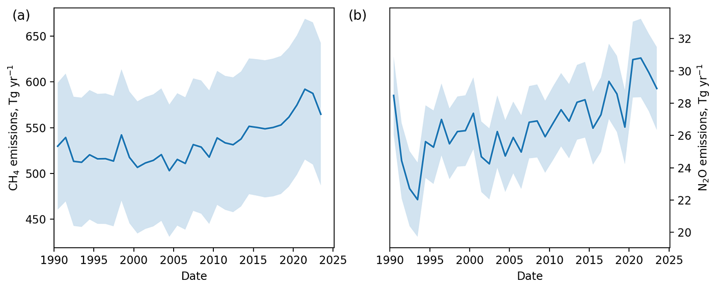
Figure 6 Global annual emissions of (a) methane and (b) nitrous oxide for 1990–2023. Shading indicated the 1σ uncertainty due to measurement repeatability, model uncertainty, calibration scale uncertainty and lifetime uncertainty.

The global mean mole fraction of methane reached 1917 ± 10 ppb in 2023, following an accelerating rate of growth since a plateau in the global mole fraction during the mid-2000s (Rigby et al., 2008). This increase in the global mole fraction is coupled with an increase in the north-south interhemispheric difference. Global emissions of methane in 2023 were 579 ± 73 Tg yr⁻¹. In 2020 these emissions were 564 ± 78 Tg yr⁻¹, which falls within the range of top-down emissions derived for methane in multiple studies, of 608 [561–650] Tg (Saunois et al., 2025). The main drivers behind the increases and times of stagnation in direct methane emissions and the resulting global mole fraction are uncertain and may come from a mixture of natural and anthropogenic source and sink processes (Nisbet et al., 2016; Schaefer et al., 2016; Rigby et al., 2017; Turner et al., 2017; Worden et al., 2017; Jackson et al., 2020; Feng et al., 2023; Zhang et al., 2023).

The global mean mole fraction of nitrous oxide reached 337 ± 2 ppb in 2023, following an increasing rate of growth since direct measurement records began. The north-south interhemispheric difference has shown substantially interannual variability but no obvious overall trend during this time. Global annual emissions reached 29 ± 3 Tg yr⁻¹ in 2023. In 2020 global emissions were 31 ± 2 Tg yr⁻¹, which is larger than the range of 26.7 [26.1–27.3] Tg yr⁻¹ (mean and range) for 2020 from four top-down approaches (Tian et al., 2024), but close to the estimate of 30.4 [29.7–31.6] Tg yr⁻¹ in Stell et al. (2022). The emissions in 2020 are within the range of bottom-up estimates of 29.1 [16.7–42.4] Tg yr⁻¹ presented in Tian et al. (2024).

6.3 Very short-lived chlorinated substances, methyl chloride and methyl bromide

Very short-lived substances (VSLSs) have total atmospheric lifetimes of less than around 6 months. Dichloromethane (CH₂Cl₂) and chloroform (CHCl₃) have natural as well as anthropogenic sources, although the natural emissions of CH₂Cl₂ are relatively minor (McCulloch, 2003; Simmonds et al., 2006). The atmospheric mole fraction of CH₂Cl₂, and its emissions, have been continuously increasing during the atmospheric record (Fig. 7 and see, e.g., Trudinger et al. (2004)). Its global mean mole fraction has approximately doubled between 2008 and 2023, when it reached 41.5 ± 1.3 ppt, which has been driven mostly by increased emissions from China (An et al., 2021). Mole fraction and emissions of CHCl₃ increased rapidly until 2015 (Fang et al., 2019), after which they fell to the levels seen in the 2000s. Perchloroethylene (CCl₂=CCl₂) has only anthropogenic sources and its atmospheric abundance and emissions have been falling since the measurement record began.

Methyl chloride (CH₃Cl) has an atmospheric lifetime of 10–11 months. It has a mixture of natural and anthropogenic sources (Rhew et al., 2000). Its atmospheric mole fraction has remained fairly constant at around 550 ppt and its emissions at 4500–5000 Gg yr⁻¹ over the measurement record. Methyl bromide (CH₃Br) has an atmospheric lifetime of 9–10 months. It has a mixture of natural and anthropogenic (foremost fumigation) sources (Laube and Tegtmeier, 2023). Its production for all applications other than quarantine and pre-shipment purposes has been phased out under the Montreal Protocol, and its atmospheric mole fraction and emissions have been declining over the measurement record (Fig. 7).

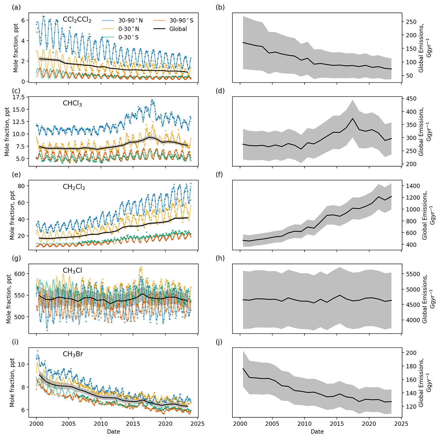
Figure 7 Semihemispheric and global mean mole fractions for (a) perchloroethylene, (c) chloroform, (e) dichloromethane, (g) methyl chloride and (i) methyl bromide. Circles show the observed semihemispheric mole fractions and the lines show the fits to these data. Their global emissions are shown in panels (b), (d), (f), (h), (j). Shading indicated the 1σ uncertainty.

7 Limitations

Whilst the data sets presented here have been extremely useful for many studies charting the atmospheric and emissions history of these substances, users should be aware of their limitations. Failure to account for these limitations could lead to erroneous conclusions being drawn from the underlying AGAGE data.

The use of a box model of atmospheric transport to estimate emissions and mole fractions is associated with numerous potential issues. Emissions estimates on scales smaller than the model resolution are not possible. However, we also find that the coarse parameterisation of atmospheric transport precludes reliable semihemispheric emissions estimates, even at the model resolution. For that reason, we do not present semihemispheric emissions estimates, only semihemispheric mole fractions (which are better constrained by the measurements themselves). Furthermore, numerous studies have shown that the use of interannually repeating meteorology can lead to specious year-to-year fluctuations in global emissions due to the lack of influence from large-scale dynamical changes (e.g., Ray et al., 2020; Montzka et al., 2021). Due to the lack of interannually varying OH and other sinks, longer term trends in emissions and year-to-year differences may be misrepresented (e.g., Rigby et al., 2008, 2017; Turner et al., 2017; Naus et al., 2019).

Currently, emission estimates are only possible in the four lowest boxes. Therefore, emissions from aircraft or other airborne sources cannot be simulated. This includes in-atmosphere production of atmospheric breakdown products, for example, the proposed production of HFC-23 due to ozonolysis of some hydrofluoroolefins (HFOs) (McGillen et al., 2023). The lack of an explicit chemistry scheme would make any such processes difficult to include at present. Following the uptake of a trace gas by the ocean, there is the possibility that this current loss process instead becomes a source (Wang et al., 2021). This effect is neglected in the model as ocean/soil uptake is only a loss process, and should not impact the compounds of interest for the foreseeable future.

The isomers of some compounds are not currently separated using the instrumentation described in Sect. 2, as noted in Table 1. For example, the isomers CFC-113 and CFC-113a are not currently separated, and the reported mole fraction is generally reported as a somewhat ill-defined combination of both isomers (Montzka et al., 2024). This issue has become more important in recent years because the more minor abundant isomer for some isomer pairs (e.g., CFC-113/a, CFC-114/a) has been increasing in the atmosphere (Western et al., 2023). Emissions and mole fraction trends for these individual isomers cannot be properly quantified at present.

The inverse method employed in this work, which constrains the emissions growth rate, is not strongly influenced by overall biases in the total magnitude of a priori emissions, compared to methods that constrain absolute emissions (Rigby et al., 2011a). However, the magnitude of the a priori growth uncertainty is informed by growth in the a priori emissions, or else chosen somewhat heuristically. Furthermore, spatial constraints are difficult to impose simultaneously with the growth constraint on emissions, as are non-negative emissions constraints. It would be preferable to employ an approach that allows physical limits to be applied to emissions and was less dependent on poorly understood uncertainties (e.g., Ganesan et al., 2014).

Since AGAGE measures trace gases at a frequency on the order of hours, a filter must be applied to provide estimates of baseline monthly mean mole fractions, which are used in combination with the box model (see Sect. 2.3). The current AGAGE statistical baseline method is simple and efficient to apply, but it can be unreliable, particularly at the beginning and end of the data set, before and after prolonged periods of instrumental downtime, during periods of poor precision, for highly polluted species/sites, or for sites that are influenced by monsoons. An alternative approach would use air histories to identify unpolluted periods and may be used in future versions (Manning et al., 2021).

Finally, our derived emissions estimates are sensitive to potential biases in the observations and model. Estimates are available for the uncertainty due to the assumed atmospheric lifetime and calibration scale, and these terms are included in our derived emissions estimates. However, for some compounds, particularly those with shorter lifetimes, unaccounted-for biases may exist because the network and model cannot resolve zonal gradients or meridional gradients within each box. For example, a difference between AGAGE and NOAA-derived dichloromethane emissions is thought to be partly due to differences in measurement locations in the Northern Hemisphere tropics between the two networks, as well as a large (∼10 %) difference in calibration scales (Carpenter and Reimann, 2014).

8 Code and data availability

All AGAGE derived data sets presented in the paper are available at https://doi.org/10.5281/zenodo.15372480 (Western et al., 2025). Users must agree to the AGAGE Data Policy, the details of which can be found when downloading the data sets. The monthly mean measurements for each site used as input to the 12-box model are available from Prinn et al. (2025) (https://doi.org/10.60718/0FXA-QF43). The 12-box model and its inversion code are available from Rigby and Western (2022a) (https://doi.org/10.5281/zenodo.6857447) and Rigby and Western (2022b) (https://doi.org/10.5281/zenodo.6857794), respectively, or from https://github.com/mrghg/py12box (last access: 8 May 2025) and https://github.com/mrghg/py12box_invert (last access: 8 May 2025).

9 Summary

The data products described here provide annual updates to the global emissions and mole fraction trends, derived from measurements from the AGAGE network, routinely published in other scientific articles and assessments. The methodology and data inputs for deriving these data sets have been described in detail in one publication for the first time. The methodology will be updated along with emerging science, including, but not limited to, updated estimates of lifetimes and updated a priori emissions estimates. The aim will be for the methodology to remain consistent with future iterations of the World Meteorological Organisation's quadrennial Scientific Assessment of Ozone Depletion and other relevant assessments.

Global emissions, mole fractions, and their growth rates derived using AGAGE measurements and a 12-box model remain in widespread use. More complex transport models combined with AGAGE measurements are likely to complement the data sets provided here (e.g., Western et al., 2024a; Liu et al., 2024), although we anticipate that the 12-box model will remain in use for many years to come, due to its efficient and ease of use in this application.