An operational SMOS soil freeze–thaw product

The Soil Moisture and Ocean Salinity (SMOS) satellite is a valuable tool for monitoring global soil freeze–thaw dynamics, particularly in high-latitude environments where these processes are important for understanding ecosystem and carbon cycle dynamics. This paper introduces the updated SMOS Level-3 (L3) Soil Freeze–Thaw (FT) product and details its threshold-based classification algorithm, which utilizes L-band passive microwave measurements to detect soil freeze–thaw transitions; this is possible due to the difference in dielectric properties between frozen and thawed soils at this frequency band. The algorithm applies gridded brightness temperature data from the SMOS satellite, augmented with ancillary datasets of air temperature and snow cover, to generate global estimates of the freeze–thaw state. A recent update to the algorithm includes improved noise reduction through temporal filtering. Validation results against in situ soil moisture and temperature measurements and comparisons to ERA5-Land reanalysis data demonstrate the ability of the product to detect the day of first freezing, an important metric for better understanding greenhouse gas fluxes and ecosystem dynamics, with improved accuracy. However, limitations remain, particularly in regions affected by radio frequency interference (RFI) and during spring melt periods, when wet snow hinders soil thaw detection. Despite these challenges, the SMOS FT product provides crucial data for carbon cycle studies, particularly in relation to methane fluxes, as soil freezing affects methane emissions in high-latitude regions. The SMOS L3FT dataset is available at https://doi.org/10.57780/sm1-fbf89e0 (ESA, 2023).

1 Introduction

More than half of the land in the Northern Hemisphere undergoes seasonal freezing and thawing each year, making it one of the most widespread environmental processes on Earth (Zhang et al., 2003). Seasonal soil freezing and thawing is not only a critical environmental phenomenon but also a key indicator of climate change and variability (Frauenfeld and Zhang, 2011; Peng et al., 2016). Soil freeze–thaw cycles are closely linked to surface temperature fluctuations and snow cover dynamics, playing an important role in regulating the Earth's energy balance (Sokratov and Barry, 2002).

Monitoring the freeze–thaw cycle is essential because it directly impacts global ecosystems, hydrology, and climate systems. As soil freezes and thaws, it drives a range of ecological processes, including carbon and nutrient cycling, soil moisture dynamics, vegetation growth, and the activity of soil organisms. Thawing periods release stored water, influencing surface runoff, groundwater recharge, and the emission of greenhouse gases such as carbon dioxide and methane (Song et al., 2017; Wagner-Riddle et al., 2017; Boswell et al., 2020; Yang and Wang, 2019; Hayashi, 2013; Nikrad et al., 2016). These emissions are particularly relevant in the context of climate change, as thawing permafrost can release significant amounts of previously trapped carbon, creating a feedback loop that accelerates global warming (Johnston et al., 2014; Knoblauch et al., 2017). The freeze–thaw cycle also has substantial implications for infrastructure, as the freezing and thawing of soil can damage buildings, roads, and pipelines due to frost heave and ground subsidence. Agriculture is similarly affected, with the timing and intensity of freeze–thaw events influencing soil fertility, crop viability, and water availability (Kreyling et al., 2008; Krogstad et al., 2022). Therefore, accurate monitoring and prediction of soil freeze–thaw cycles are crucial not only for understanding natural ecosystems but also for mitigating risks and optimizing land-use practices in affected regions.

Global monitoring of the soil freeze–thaw cycle is vital for advancing our understanding of ecosystem dynamics, refining climate models, and managing natural resources. High-latitude and high-altitude regions are particularly sensitive to freeze–thaw cycles, where even minor changes can disproportionately affect local environments and contribute to broader global changes (Shiklomanov, 2012). L-band passive microwave remote sensing is particularly effective for detecting soil freeze–thaw transitions due to the high contrast in permittivity between liquid water and ice at L-band frequencies (1–2 GHz) (Rautiainen et al., 2014). Compared to higher frequencies, the L-band allows for deeper penetration into the soil, enabling observations several centimetres beneath the surface. As measurement frequency increases, the proportion of the signal originating from the soil decreases, with higher-frequency bands interacting more strongly with surface vegetation or snow cover in winter. These subsurface observations are critical, as the significant difference in the dielectric constant between frozen and thawed soil results in pronounced changes in soil emissivity that L-band radiometers can effectively detect, ensuring high sensitivity to freeze–thaw dynamics.

Over the past decades, several global data products have been developed to monitor soil freeze–thaw cycles. These include the Freeze–Thaw Earth System Data Record (FT-ESDR) (Kim et al., 2017), the Soil Moisture and Ocean Salinity Level-3 Soil Freeze–Thaw (SMOS L3FT) product (ESA, 2023; Rautiainen et al., 2016), and the Soil Moisture Active Passive Freeze–Thaw (SMAP FT) product (Derksen et al., 2017). The FT-ESDR combines data from the Advanced Microwave Scanning Radiometer (AMSR-E) on NASA’s Aqua satellite and the SSMIS on the Defense Meteorological Satellite Program platforms, providing a long-term, consistent dataset for global monitoring of freeze–thaw cycles, particularly useful for analysing inter-annual variability and long-term trends. However, the FT-ESDR relies on high-frequency (36.5 GHz) radiometer data, primarily sensing the freeze–thaw status at the very surface of the landscape, and is therefore more affected by the vegetation and snow cover. In contrast, the SMAP FT and SMOS L3FT products are based on low-frequency passive L-band brightness temperatures, which are more sensitive to thermal emission originating from the soil. Although the SMAP mission originally included an active L-band radar, the radar instrument unfortunately failed shortly after the mission’s launch.

This paper describes the updated SMOS L3FT algorithm and introduces the dataset to the community (ESA, 2023). The SMOS L3FT product has been publicly available since 2018. Developed by the Finnish Meteorological Institute in collaboration with GAMMA Remote Sensing, Switzerland, the product is accessible through the European Space Agency (ESA) SMOS and the Finnish Meteorological Institute (FMI) dissemination services. In November 2023, the SMOS L3FT product underwent a major processor update from version 2 to version 3, with all data reprocessed.

2 Data

2.1 Data used for the soil freeze and thaw detection

2.1.1 SMOS brightness temperatures

The ESA SMOS mission (Kerr et al., 2010), launched in 2010, was the first satellite mission to provide continuous L-band observations covering the whole globe. For the SMOS L3FT product, the primary input data are the CATDS (Centre Aval de Traitement des Données SMOS) level-3 brightness temperatures (L3TB) dataset, version 331 (Al Bitar et al., 2017; CATDS, 2024). The L3TB data are in the ground polarization frame, with horizontal (H) and vertical (V) linear polarizations, and are provided in the Equal-Area Scalable Earth 2 (EASE-2) grid (Brodzik et al., 2012) with a polar projection at a 25 km × 25 km grid cell size. On each overpass, SMOS measures an incidence angle profile of the brightness temperature. In the L3TB data, the profiles are averaged into incident angle bins with 5° intervals. Daily CATDS files include all swaths observed over the Northern Hemisphere. The variables used are the H and V polarized brightness temperatures, their standard deviations and radiometric accuracies, the number of views, the number of views suspected to be affected by radio frequency interference (RFI), the observation acquisition times, and the incidence angles relative to nadir. The SMOS L3FT algorithm uses only data from the incidence angle bin of 50–55°.

2.1.2 Two-metre air temperature

Daily air temperature data at 2 m above ground level are provided by the European Centre for Medium-Range Weather Forecasts (ECMWF). The operational L3FT processor utilizes the Atmospheric Model High-Resolution 10 d Forecast data from ECMWF’s real-time forecast system. During reprocessing, the near-real-time air temperature data are replaced with the corresponding air temperature data from the ERA5-Land reanalysis, which are available with a latency of up to 1 month (Muñoz Sabater et al., 2021; Muñoz Sabater, 2019). The most recent reprocessing was performed in October 2023, and all data after 10 October 2023 have been processed using ECMWF near-real-time data. Both the operational 10 d high-resolution forecasts and the ERA5-Land reanalysis from ECMWF are provided on a grid with a spatial resolution of 0.1° × 0.1° (approximately 11.1 km × 11.1 km at the Equator and 11.1 km × 5.6 km at 60° latitude), offering daily temperature values at 6 h intervals (0, 6, 12 and 18 h). The SMOS L3FT processor calculates the daily mean from these ECMWF air temperatures. The data are reprojected to the EASE-2 grid and resampled to a spatial resolution of 25 km × 25 km using the nearest-neighbour interpolation method.

2.1.3 Snow extent

The SMOS L3FT algorithm uses the global snow extent data produced by the United States National Ice Center (USNIC) using the Interactive Multisensor Snow and Ice Mapping System (IMS) (U.S. National Ice Center, 2008). These IMS Daily Northern Hemisphere Snow and Ice Analysis data, originally in 4 km resolution with polar stereographic projection, are reprojected to the EASE-2 grid at 25 km × 25 km resolution using the majority interpolation method. Although IMS provides daily global snow extent, its quality may be affected by persistent cloud cover and polar night conditions, which limit the availability of optical observations. In such cases, the IMS algorithm relies more on passive microwave inputs and temporal persistence from previous days’ estimates (U.S. National Ice Center, 2008; Helfrich et al., 2019). Given the coarse spatial resolution of the SMOS L3FT product, these limitations are not considered critical for our application.

2.2 Data used for the validation

2.2.1 Soil moisture and soil temperature

The soil moisture (SM) and soil temperature (ST) data are obtained from the International Soil Moisture Network (ISMN) (Dorigo et al., 2011, 2021). Data are available from over 70 networks worldwide, seven of which provide near-real-time updates. Here, ISMN data from six different networks are used to validate the SMOS freeze–thaw product. We use only data from those stations that measure both SM and ST from the top surface layer, at depths of 5 cm and/or 10 cm. These networks include SNOTEL – Snow Telemetry Network (Leavesley et al., 2008), SCAN – Soil Climate Analysis Network (Schaefer et al., 2007), USCRN – U.S. Climate Reference Network (Bell et al., 2013), RISMA – Real-Time In Situ Soil Monitoring for Agriculture (Ojo et al., 2015), BNZ LTER – Bonanza Creek Long-Term Ecological Research, and FMI – Finnish Meteorological Institute soil moisture and soil temperature observations (Ikonen et al., 2016, 2018).

2.2.2 ERA5-Land reanalysis data

The ECMWF ERA5-Land global atmospheric reanalysis dataset provides a consistent and long-term record of meteorological parameters over land surfaces (Muñoz Sabater et al., 2021). We used the air temperature at 2 m, soil temperature in layer 1 (0–7 cm depth), and snow depth. The data, provided on a 0.1°×0.1° latitude–longitude grid, are reprojected to the 25 km × 25 km EASE-2 grid used by the SMOS L3FT product. This is done using the Geospatial Data Abstraction Library (GDAL), with average resampling applied during resolution matching to ensure consistency with the SMOS grid.

2.2.3 Land cover

The ESA CCI Land Cover time series v2.0.7 (1992–2015) data (ESA, 2017), originally provided at 300 m spatial resolution, are used to define the land cover distribution on the EASE-2 grid. The land cover classes were aggregated from the original 23 classes into six classes: agriculture, forest, low vegetation, wetland, open water, and other (permanent ice, barren, urban). This aggregated land cover information was then regridded to the 25 km EASE-2 grid and used during the validation process to determine whether the land cover class at each in situ sensor location represented the larger EASE-2 grid cell.

3 SMOS freeze and thaw (FT) retrieval algorithm

3.1 Algorithm outline

The SMOS FT detection algorithm is based on the physical principle that L-band brightness temperatures vary significantly between frozen and thawed soils due to the distinct differences in their dielectric properties. Thawed soil contains liquid water, which has a much higher dielectric constant (ϵ’≈90) at the L-band than the ice in frozen soil (ϵ’≈3.2) (Mätzler et al., 2006). This large dielectric contrast directly influences the soil's emissivity and, consequently, the brightness temperature detected by the satellite.

As predicted by Fresnel's equations as well as by empirical observations (Rautiainen et al., 2014), the strong decline of free liquid water during soil freezing has two effects: first, both horizontal and vertical emissivities are increased, leading to an increase in the corresponding brightness temperatures. Second, the difference between horizontal and vertical emissivities is decreased, resulting in a reduction in the polarization contrast. By contrast, thawed soils – due to the presence of liquid water – exhibit lower emissivities and a larger polarization difference. Notably, dry and frozen soils behave similarly from a dielectric standpoint, causing similar effects on L-band brightness temperatures.

To detect the FT state of the soil, the algorithm computes the normalized polarization ratio (NPR), which we denote by Υ and is defined as

$$\begin{array}{}\text{(1)}& \mathrm{{\rm Y}}\stackrel{\mathrm{def}}{=}{\displaystyle \frac{T_{\mathrm{B}}^{\mathrm{V}}-T_{\mathrm{B}}^{\mathrm{H}}}{T_{\mathrm{B}}^{\mathrm{V}}+T_{\mathrm{B}}^{\mathrm{H}}}},\end{array}$$

where $T_{\mathrm{B}}^{\mathrm{V}}$ and $T_{\mathrm{B}}^{\mathrm{H}}$ are the vertically and horizontally polarized brightness temperatures, respectively. NPR reflects both the absolute level of emissivities and their polarization contrast, making it a sensitive indicator of freeze–thaw transitions. The conceptual motivation for using NPR can be understood by considering the idealized case of a bare soil surface, for which the brightness temperature can be expressed as

$$\begin{array}{}\text{(2)}& T_{\mathrm{B}}^{\mathrm{pol}}=(\mathrm{1}-{\mathrm{\Gamma }}^{\mathrm{pol}})T_{\mathrm{soil}}+{\mathrm{\Gamma }}^{\mathrm{pol}}{T}_{\mathrm{B},\mathrm{sky}}.\end{array}$$

Omitting the downwelling brightness temperature T_B,sky and substituting Eq. (2) into Eq. (1) eliminates the effect of soil's physical temperature T_soil, leaving only the dielectric effect. Ideally, this insensitivity to physical temperature variations allows robustly capturing changes in soil moisture and FT transitions without the need for an explicit temperature correction. Figure 1 shows the modelled effect of the changing soil permittivity to the NPR at the used observation angle θ=52.5°, following Fresnel's law for smooth interface.

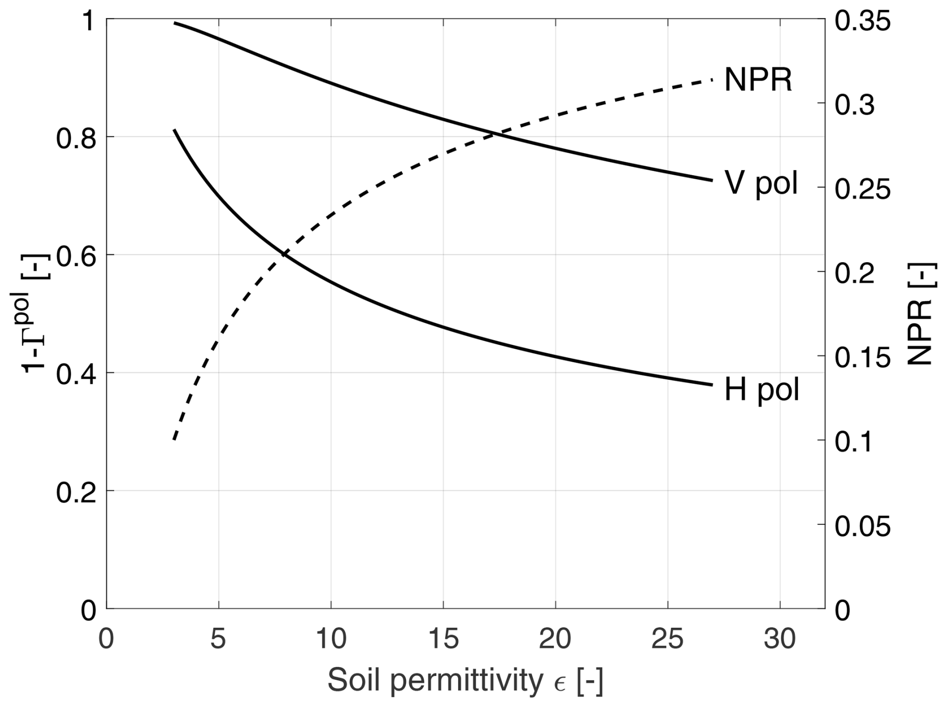
Figure 1 Soil's emissivity 1−Γ^pol(ε) for vertical and horizontal polarizations (solid line; left y axis) and the corresponding normalized polarization ratio (dashed line; right y axis) as a function of the soil's relative permittivity ε.

However, in practice, the idealized assumptions represented by Eq. (2) and Fig. 1 do not fully hold. Surface roughness, vegetation and forest cover, snow, and sub-pixel heterogeneity within the SMOS footprint all act to dampen the sensitivity of brightness temperature to soil permittivity changes. These factors reduce the interpretability of the polarization-dependent brightness temperature response and introduce geophysical noise that can be misclassified as freeze or thaw. As a result, the algorithm must be designed to tolerate such uncertainties while remaining sensitive to actual transitions in the soil freeze–thaw state.

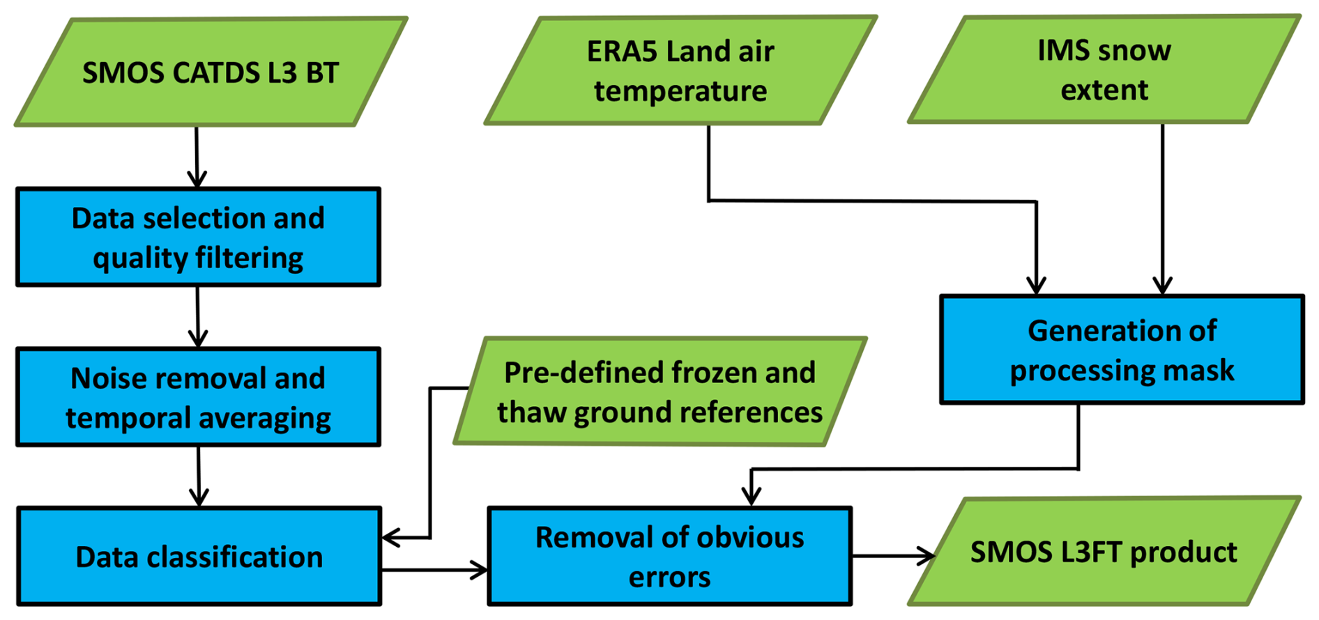
Building on this physical rationale, the algorithm applies a threshold-based classification to determine the soil freeze–thaw state from the observed NPR values. Each Υ is compared to empirically established frozen and thawed soil reference values, denoted by Υ_fr and Υ_th, respectively. The resulting soil state estimates are further regularized by air temperature reanalysis data. The algorithm workflow scheme is shown in Fig. 2 and described in detail in the sections below. As mentioned earlier, the SMOS FT algorithm primarily relies on CATDS L3 brightness temperature data as its main input. The ascending and descending orbits are processed separately, resulting in two L3FT estimates for the two orbits.

Figure 2 The SMOS soil FT detection algorithm workflow.

3.2 Data selection and quality filtering

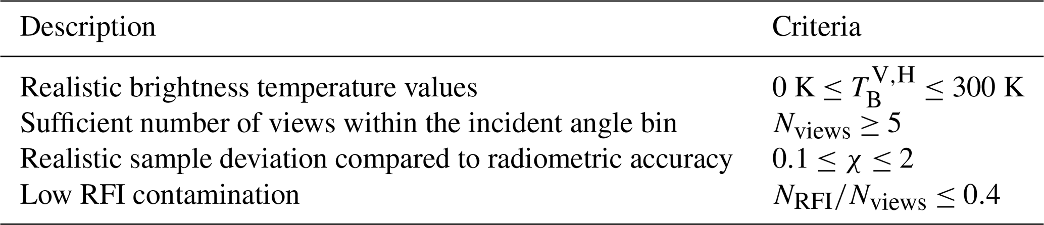
The brightness temperature measurements that are suspected to have reduced quality are filtered out. The SMOS L3FT processor uses CATDS L3TB data, which are already averaged within incidence angle bins; hence, the quality flags, including the suspected RFI proportion, are interpreted as summary statistics, and individual brightness temperature measurements are no longer accessible at this stage. Table 1 summarizes the quality filtering criteria. First, the brightness temperature values should be within the physically meaningful range. In the context of FT detection, values above 300 K can be omitted. Second, it is required that the incident angle bin contains at least five measurements. Third, the ratio

$$\begin{array}{}\text{(3)}& \mathit{\chi }={\displaystyle \frac{T{}_{\mathrm{B}}\mathrm{deviation}}{T{}_{\mathrm{B}}\mathrm{accuracy}}}\end{array}$$

between the sample standard deviation of the measurements and the average radiometric accuracy within the incident angle bin is expected to be bounded both from above and below with values of 2 and 0.1, respectively. Fourth, the proportion of measurements suspected to be contaminated by RFI within the incident angle bin must be less than 40 %.

Table 1 Data filtering criteria in the SMOS L3FT processor.

3.3 Noise removal and temporal averaging

The individual SMOS L3 brightness temperatures, although averaged over the incident angle bin, contain noise that hinders the FT detection. To remove noise from the NPR time series computed from the L3TB, a temporal filtering is performed. In the SMOS L3FT processor, a simple Kalman filtering approach is used (Kalman, 1960; Särkkä, 2013). Every grid cell is filtered independently from every other, and the time series from a given grid cell is modelled as a dynamic linear model; hence,

$$\begin{array}{}\text{(4)}& \left\{\begin{array}{ll}\mathrm{{\rm Y}}\left(t_k\right)& =\mathrm{{\rm Y}}\left(t_{k-\mathrm{1}}\right)+W_k,\\ {\mathrm{{\rm Y}}}_{\mathrm{L}\mathrm{3}\mathrm{TB}}\left(t_k\right)& =\mathrm{{\rm Y}}\left(t_k\right)+V_k,\end{array}\right.\end{array}$$

where Υ(t_k) denotes the true physical NPR at time instance t_k and Υ_L3TB(t_k) denotes the noisy NPR that is computed from the L3 brightness temperatures at time t_k by Eq. (1). W_k and V_k are the observation and model noise terms at time t_k, which were modelled as Gaussian random variables:

$$\begin{array}{}\text{(5)}& \left\{\begin{array}{ll}{W}_k& \sim \mathcal{N}(\mathrm{0},w_k^{\mathrm{2}}),\\ V_k& \sim \mathcal{N}(\mathrm{0},v_k^{\mathrm{2}}).\end{array}\right.\end{array}$$

The NPR observation noise variance $v_k^{\mathrm{2}}$ and the process noise variance $w_k^{\mathrm{2}}$ were estimated as follows:

$$\begin{array}{}\text{(6)}& \left\{\begin{array}{ll}{v}_k^{\mathrm{2}}& =\frac{\mathrm{var}{T}_{\mathrm{B}}^{\mathrm{V}}\left(t_k\right)+\mathrm{var}{T}_{\mathrm{B}}^{\mathrm{H}}\left(t_k\right)}{{\left(T_{\mathrm{B}}^{\mathrm{V}}\left(t_k\right)+T_{\mathrm{B}}^{\mathrm{H}}\left(t_k\right)\right)}^{\mathrm{2}}},\\ w_k^{\mathrm{2}}& ={\mathit{\vartheta }}^{\mathrm{2}}(t_{k-\mathrm{1}}-t_k),\end{array}\right.\end{array}$$

where ϑ is a tuning parameter, T_B(t_k) refers to the brightness temperature values at time t_k, and var(⋅) refers to the error variance of the brightness temperatures, which are provided in the data. The Kalman filter provides an optimal estimate of Υ(t_k) from the noisy time series Υ_L3TB(t_k), balancing the noisy observations with their uncertainties to improve the signal quality. Figure 3 shows an example of the observed time series before and after applying the Kalman filter. The advantage of the Kalman filtering approach over, e.g., a running mean is that the observations are weighted according to their uncertainty; in addition, the filtering parameter ϑ can be estimated from an observed time series by maximizing the likelihood of the observed time series with respect to ϑ (see, e.g., the book by Särkkä, 2013). The estimation is performed for the EASE-2 grid cell over Sodankylä, Finland, one of the applied validation sites (Ikonen et al., 2016), and the obtained value ϑ₀=0.003 is used globally.

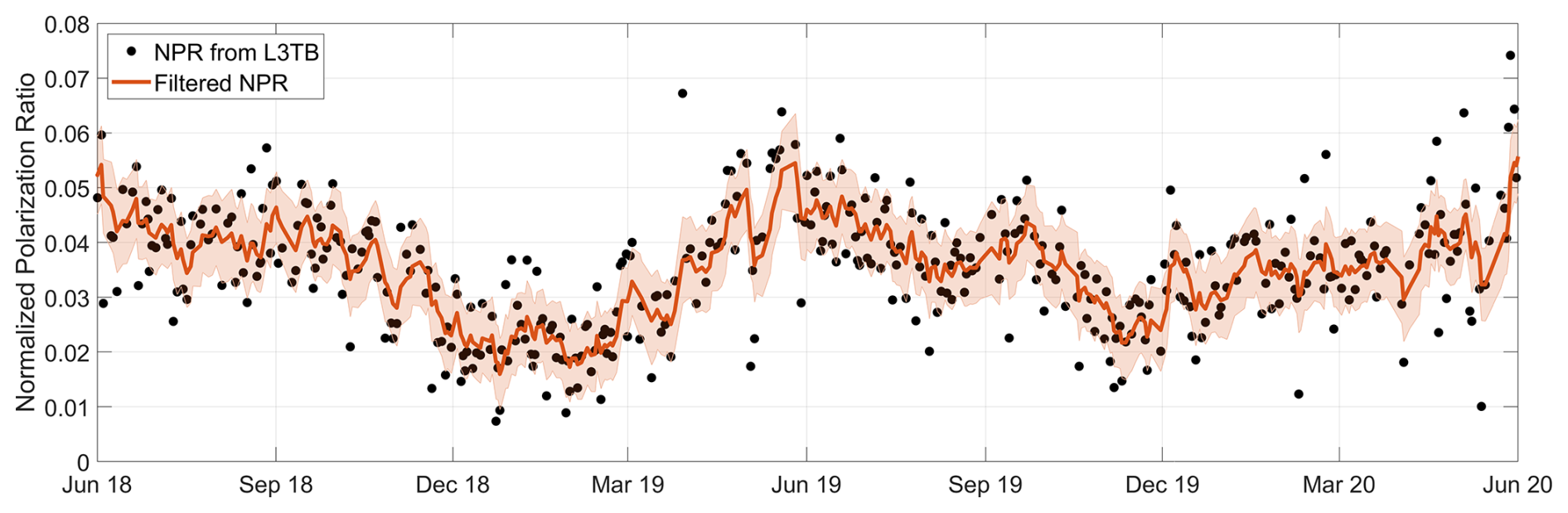
Figure 3 Time series of the non-filtered (computed from the L3TB swath data) and the filtered normalized polarization ratio from the EASE2.0 grid cell containing the Sodankylä validation site.

3.4 Frozen and thawed ground references

NPR varies between grid cells due to differences in land cover, soil properties, vegetation cover, and environmental conditions. As a result, each cell exhibits unique frozen and thawed soil references: Υ_fr and Υ_th. To detect the freeze–thaw transitions, we scale the observed NPR signal:

$$\begin{array}{}\text{(7)}& {\mathrm{{\rm Y}}}_{\mathrm{sc}}={\displaystyle \frac{{\mathrm{{\rm Y}}}_{\mathrm{th}}-\mathrm{{\rm Y}}}{{\mathrm{{\rm Y}}}_{\mathrm{th}}-{\mathrm{{\rm Y}}}_{\mathrm{fr}}}},\end{array}$$

where Υ_sc is the scaled NPR. Note that Υ_fr and Υ_th are specific to each grid cell and that they are empirically derived from the L3TB time series in conjunction with two auxiliary datasets: ERA5-Land air temperature and IMS snow extent. By scaling the Υ values in this way, the algorithm adapts to the local conditions of each cell, enabling accurate determination of the soil state from the current observations.

The methodology used to define the reference values from the NPR time series is described below. If the daily mean air temperature was below −3 °C and there was snow cover, the data were eligible for the frozen soil reference. Similarly, if the snow melt-off occurred at least 28 d ago and the daily air temperature was above +3 °C, the data were eligible for the thawed soil reference. This decision logic is shown in Fig. 4. Reference values were derived from data collected between 1 January 2014 and 4 September 2023, with the end date limited by the availability of ECMWF ERA5-Land data at the time of reprocessing. The first years of data were excluded due to the higher presence of RFI. From the selected period, all eligible frozen and thawed reference data were collected, and the 50 most extreme values were identified. The median of these values was used to define the frozen Υ_fr and thawed Υ_th reference values.

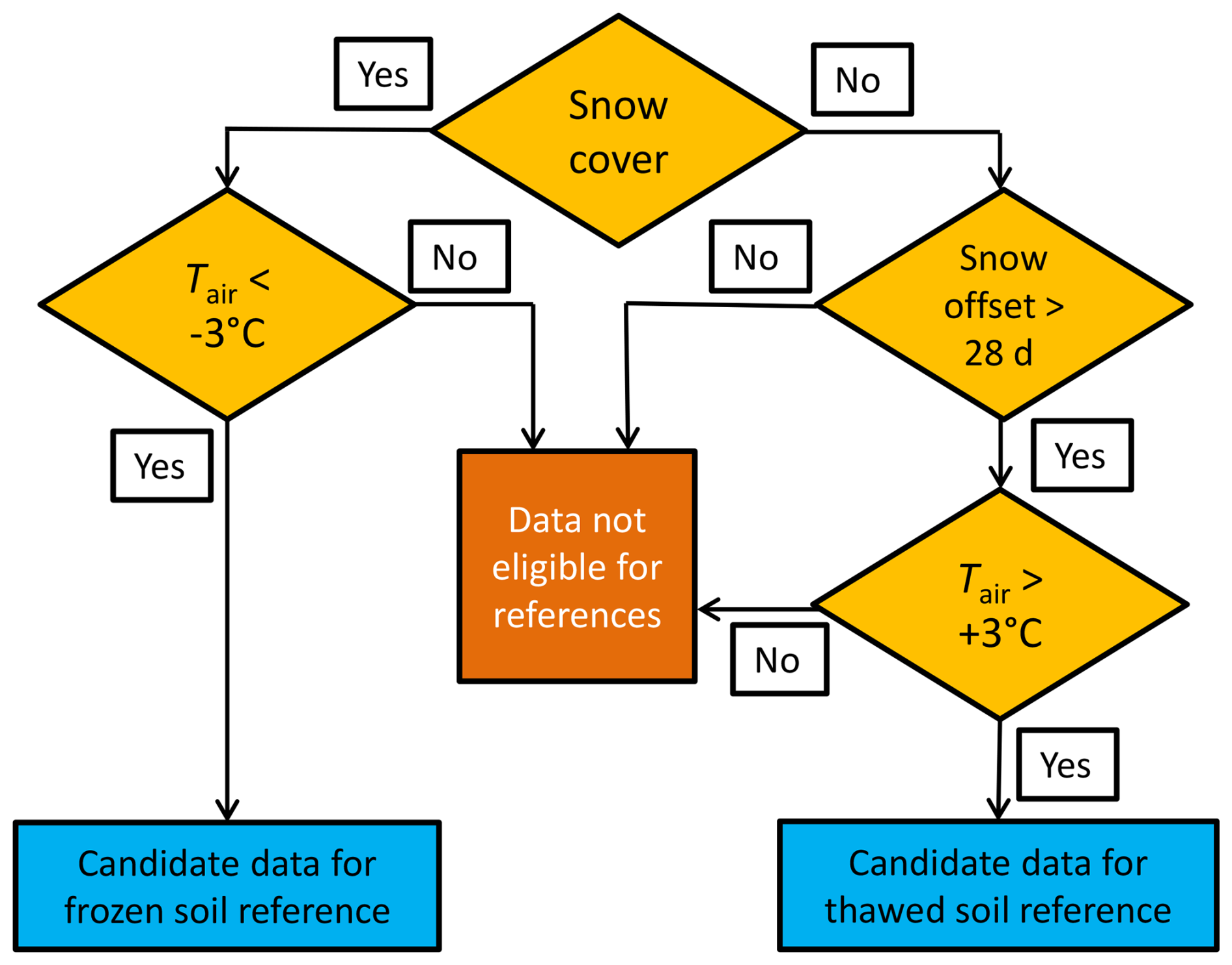
Figure 4 The logic for selecting the candidate data for the frozen and thawed soil references.

3.5 Data classification

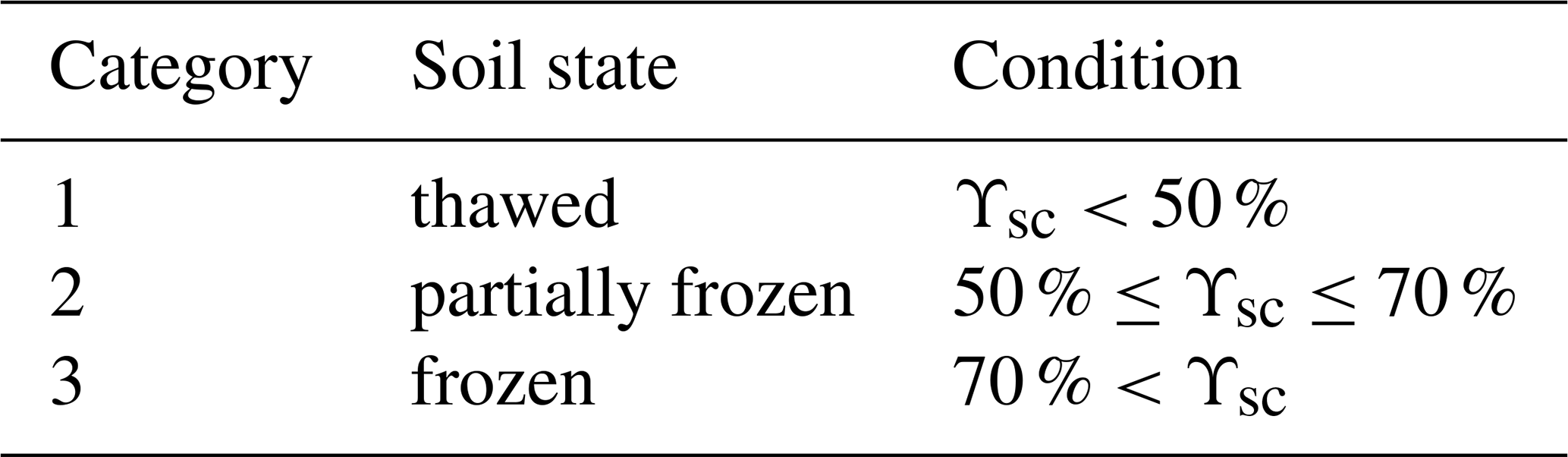
The FT class was estimated from the scaled NPR value Υ_sc according to Table 2. The thresholds of 50 % and 70 % were acquired in previous studies by fitting the scaled NPR value to frost tube observations in Finland (Rautiainen et al., 2016).

Table 2 Thresholds for the soil state categories with respect to the parameter A and with respect to frozen and thawed soil references.

3.6 Removal of obvious errors and the processing mask

Even after the preprocessing steps for filtering the observational data, the initial freeze–thaw (FT) classification based on the scaled NPR value may contain errors, in particular over regions where some residual RFI is present or where the separation of frozen and thawed references is small. Some of the obviously erroneous ground condition classifications can be mitigated using the auxiliary data: ECMWF air temperature and IMS snow extent. A processing mask (PM) was generated using these auxiliary data to estimate the season occurring in each grid cell. Additionally, the previously defined PM state restricted the selection of the new value. PM contains eight different values for four seasons (two for each). They are described in Table 3 with the selection criteria and the allowed transitions.

Table 3 The nine values of processing mask PM(t) for time t (day), the criteria for their conditions, the respective seasons, and the allowed transitions PM(t) ⟶ PM(t+1). The variables T_air and $\stackrel{\mathrm{‾}}{T_{\mathrm{air}}}$ denote the daily mean and 10 d mean air temperatures, respectively.

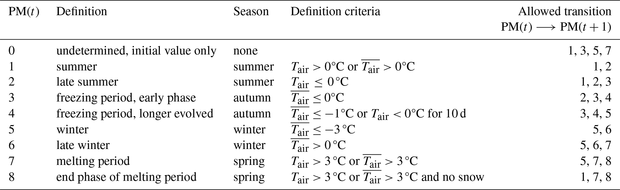
PM affects the final estimate according to the following rules: (1) if PM(t) is 3, 4, 7, or 8 (indicating freezing and melting periods), the mask has no effect. (2) If PM(t) is 1 or 2 (indicating a summer period), all FT state estimates are forced into the thawed soil category. (3) During the winter period (when PM(t) is 5 or 6), the mask prevents the soil state from changing towards the thawed state. However, neither the frozen state nor the partially frozen state is forced.

4 Validation

4.1 Validation with in situ data

The soil freeze–thaw (FT) estimates were compared against the ISMN SM and ST data. The scale mismatch between satellite-based and in situ observations presents significant challenges when interpreting the comparison results. In situ sensors measure the soil state at a single point, whereas SMOS observations represent an area with an effective footprint of 30–50 km, depending on the location within the snapshot scene (McMullan et al., 2008; Kerr et al., 2010).

Temporal uncertainty also affects the comparison because SMOS does not always provide daily observations for a given location. Due to its orbital configuration and data gaps caused by radio frequency interference (RFI), particularly in Eurasia (Oliva et al., 2016), the satellite may miss critical transition days. This can delay or obscure the detection of the actual freeze onset. In contrast, in situ data are typically available at hourly resolution, allowing precise identification of freezing events. Although SMOS and in situ data can be time-matched when observations are available, the discontinuous temporal sampling of SMOS introduces uncertainty that must be considered in the comparison.

The SMOS FT product estimates the soil state at three levels (Table 2). To compare the SMOS FT estimates against the in situ data, a similar parameter indicating the soil state at the sensor location needs to be defined from the in situ observations. The soil state at the in situ sensor locations was quantified using a soil FT index (SFTI). This index was derived by analysing the relationship between the measured soil volumetric liquid water content (LWC) and soil temperature, represented by the soil freezing characteristic curve (SFCC). A simultaneous decrease in both LWC and temperature indicates soil freezing, whereas an increase in both parameters suggests soil thawing. This method is based on the approach developed by Pardo Lara et al. (2020) and is further elaborated and explained in detail by Cohen et al. (2021). The SFTI is a site-specific metric representing the soil state, with values ranging from 0 to 1, where 0 corresponds to thawed soil and 1 to fully frozen soil. For comparison purposes, we used three SFTI thresholds: 50 %, 70 %, and 90 %. The SFTI time series were then converted into three sets of binary data, each indicating whether the soil at the sensor locations was classified as either frozen or thawed based on these threshold values, with higher thresholds reflecting a stronger indication of frozen conditions. These binary datasets were compared with the SMOS FT estimates. The day of first freezing (DoFF) in autumn was chosen as the comparison parameter because it plays a critical role in greenhouse gas (GHG) emissions, particularly methane (Arndt et al., 2019; Tenkanen et al., 2021). Previous studies have shown that soil FT estimates derived from L-band passive microwave data are most accurate during the autumn and cold winter periods. In the spring, direct observations from the ground, even at L-band frequencies, are effectively blocked by the wet snow layer (Roy et al., 2015; Rautiainen et al., 2016). As a result, the SMOS FT estimates during this period often reflect the condition of the snowpack (e.g. presence of wet snow) rather than the actual soil thawing. Although in situ sensors provide accurate information about the soil state itself, the springtime SMOS FT signal cannot be directly interpreted as soil thaw, which limits its suitability for soil FT validation during this season.

DoFF is defined here as the first day in autumn that is followed by at least 5 consecutive days of frozen soil. For SMOS data, an additional condition was applied: five consecutive observations must estimate a frozen soil state. Due to SMOS’s orbit configuration, global coverage is achieved every 3 d, with combined ascending and descending overpasses enabling daily observations north of approximately 60° N (Kerr et al., 2010). However, because the SMOS L3FT retrievals are computed separately for each orbit, near-daily coverage for either ascending or descending observations is attained only at latitudes above ∼ 65° N. This is also evident in the SMOS observation frequency map shown in Fig. 8. Additionally, data quality filtering, especially due to radio frequency interference (RFI), further reduces the effective observation frequency, particularly in Eurasia. As a result, the five observations required to confirm freezing typically span 5–15 d, depending on latitude and data quality. This limited temporal resolution may delay the DoFF detection relative to the actual onset of soil freezing. To account for temporal uncertainty due to irregular SMOS sampling, we define the day of first potential freezing (DoFPF) as the last observation that still indicated a thawed state before the confirmed onset of freezing (DoFF). This ensures that the actual transition lies between DoFPF and DoFF. The period between these two dates represents the time during which SMOS FT estimates indicate the onset of soil freezing in autumn. Similarly, DoFF was determined from in situ SFTI measurements using the three previously selected thresholds (50 %, 70 %, and 90 %) for comparison.

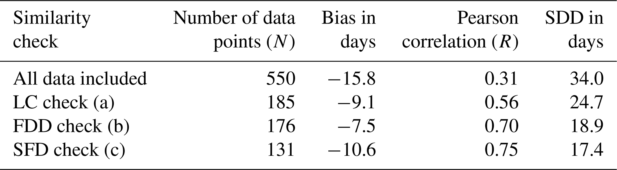
Figure 5 compares the day of first freezing (DoFF) derived from in situ measurements with SMOS freeze–thaw (FT) product estimates, showing results for both ascending and descending orbits. The error bars indicate the range of uncertainty for both the SMOS FT product and the in situ measurements in estimating DoFF. For SMOS, the error bars extend from the day of first potential freezing (DoFPF) to the day of first freezing (DoFF), with the midpoint marker representing the average estimate. The SMOS FT error bar reflects the variability in satellite observation times, which can span multiple days due to the satellite’s overpass frequency. For in situ measurements, the error bars reflect the range between the 50 % and 90 % thresholds, with the marker also set at the midpoint. The error bars for in situ data reflect the variability in defining the exact timing of freezing based on the SFTI thresholds. A wider range between the 50 % and 90 % thresholds suggests more gradual soil freezing, introducing greater uncertainty into the timing of DoFF. In contrast, narrower error bars indicate a more abrupt freeze transition and therefore a more certain timing estimate at the sensor location. The bias, Pearson correlation (R), and standard deviation of difference (SDD) values were calculated for the midpoints. For SMOS, the result represents the effective FT state within the grid cell. For the in situ measurements, the data may be from only one sensor location, or there may be several locations around the grid cell. If multiple sensors are included, the SFTI data were averaged considering the land class information of the sensor locations and the land class distribution of the associated grid cell. Prior to comparison, in situ data were excluded if they were not representative of the larger EASE-2 grid cells. Several criteria for representativeness were given: (a) the land cover similarity check with the aggregated land cover data (Sect. 2.2.3) – the land cover on at least one sensor location had to be the same as the dominant land cover within the EASE-2 grid cell, the total land cover classes where the sensors were located had to cover 70 % or more of the EASE-2 grid cell, and a maximum allowable fraction of 5 % within a grid cell was permitted for open water. Likewise, the combined fraction of all types in the “other” category (permanent ice, barren land, and urban areas) could not exceed 5 %. (b) The freezing degree day (FDD) check – for each EASE-2 grid cell and for each autumn/early winter period, FDDs were calculated using the ERA5-Land air temperature data. If the FDDs were 0 °C or more than 500 °C (i.e. the cumulative sum of daily freezing degree days) at the time when the in situ sensor indicated frozen ground (at the 70 % threshold), the in situ sensor was considered unrepresentative of the entire grid cell area. (c) The soil frost depth (SFD) check – we estimated the expected average soil frost depth for each grid cell using a simple regression model based on ERA5-Land air temperature and snow depth data. The change in soil frost depth (ΔSFD) was estimated using the regression model from Gregow et al. (2011):

$$\begin{array}{}\text{(8)}& \mathrm{\Delta }\mathrm{SFD}=a_{\mathrm{1}}+a_{\mathrm{2}}\cdot {\text{FDD}}_{\mathrm{10}}+a_{\mathrm{3}}\cdot d_{\mathrm{snow}},\end{array}$$

where snow depth d_snow is in centimetres and the regression coefficients are a₁=0.591 cm, a₂=0.079 cm °C⁻¹, and $a_{\mathrm{3}}=-\mathrm{0.161}$. FDD₁₀ is the 10 d freezing degree days:

$$\begin{array}{}\text{(9)}& {\text{FDD}}_{\mathrm{10}}=\sum _{i=\mathrm{1}}^{\mathrm{10}}max(\mathrm{0},-T_i),\end{array}$$

and T_i is the daily average temperature on day i (in °C). Similarly, if the estimated frost depth was 0 cm or more than 100 cm when the in situ sensor indicated soil freezing (70 % threshold), the in situ sensor could not represent the entire grid cell around it. As a result of the quality checks, the number of data points (N) in the comparison exercise was reduced from 550 to 131.

Tables 4 and 5 present the comparison metrics at various representativeness levels for SMOS DoFF and in situ SFTI DoFF using the 50 % threshold. The largest reduction in data points occurred during the land class similarity check (criterion a), which also significantly improved the metrics. The FDD check (criterion b) identified nine additional cases where the in situ soil freezing estimates clearly contradicted the ERA5-Land data, resulting in noticeable improvements in the statistics. The final criterion (c), which involved comparison against model-based soil frost depth information, excluded 45 more cases and led to slight further improvements in the results.

Table 4 The comparison result metrics for ascending orbit SMOS DoFF and in situ SFTI DoFF using the 50 % threshold. The representativeness checks (land class (LC), FDD, and SFD) were applied cumulatively: for example, “SFD check (c)” includes only those data points that passed both the LC (a) and FDD (b) checks.

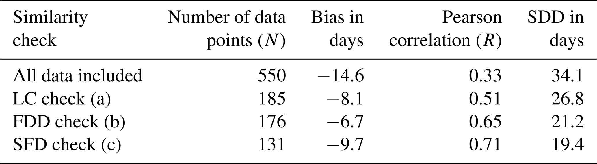
Table 5 The comparison result metrics for descending orbit SMOS DoFF and in situ SFTI DoFF using the 50 % threshold. The representativeness checks (LC, FDD, and SFD) were applied cumulatively.

The metrics shown in Fig. 5 demonstrate the performance of the SMOS FT product. Note that these metrics are based on the midpoint values of the uncertainty ranges shown in the figure: for SMOS, the midpoint between the day of first potential freezing (DoFPF) and the day of first freezing (DoFF), and for the in situ data, the midpoint between the 50 % and 90 % SFTI thresholds. This differs from the comparison metrics in Tables 4 and 5, which are computed directly between SMOS DoFF and the in situ DoFF derived from the 50 % SFTI threshold.

For the descending orbits (Fig. 5b), the bias is −6.3 d, with a Pearson correlation of 0.71 and an SDD of 18.6 d. This indicates that, on average, the SMOS product estimates the day of first freezing later than in situ measurements. The relatively high correlation reflects strong agreement between SMOS estimates and in situ data, suggesting that the product reliably captures the freeze–thaw transition in autumn, despite the temporal and spatial differences between satellite and in situ observations. The SDD highlights the deviation between the two datasets, which is typical considering the challenges of matching large-scale satellite observations to point-based in situ sensors.

For the ascending orbits (Fig. 5a), the bias is −5.0 d, with the same Pearson correlation of 0.71 and an SDD of 19.2 d. This suggests that ascending orbits tend to estimate freezing later than in situ measurements but 1.3 d earlier compared to estimates from the descending orbit. This earlier detection of freezing by ascending orbits aligns with the SMOS satellite's sun-synchronous orbit configuration, where ascending orbits capture morning conditions (06:00 local time) and descending orbits capture evening conditions (18:00 local time). The colder morning temperatures likely cause soil freeze–thaw transitions to be detected slightly earlier during ascending passes.

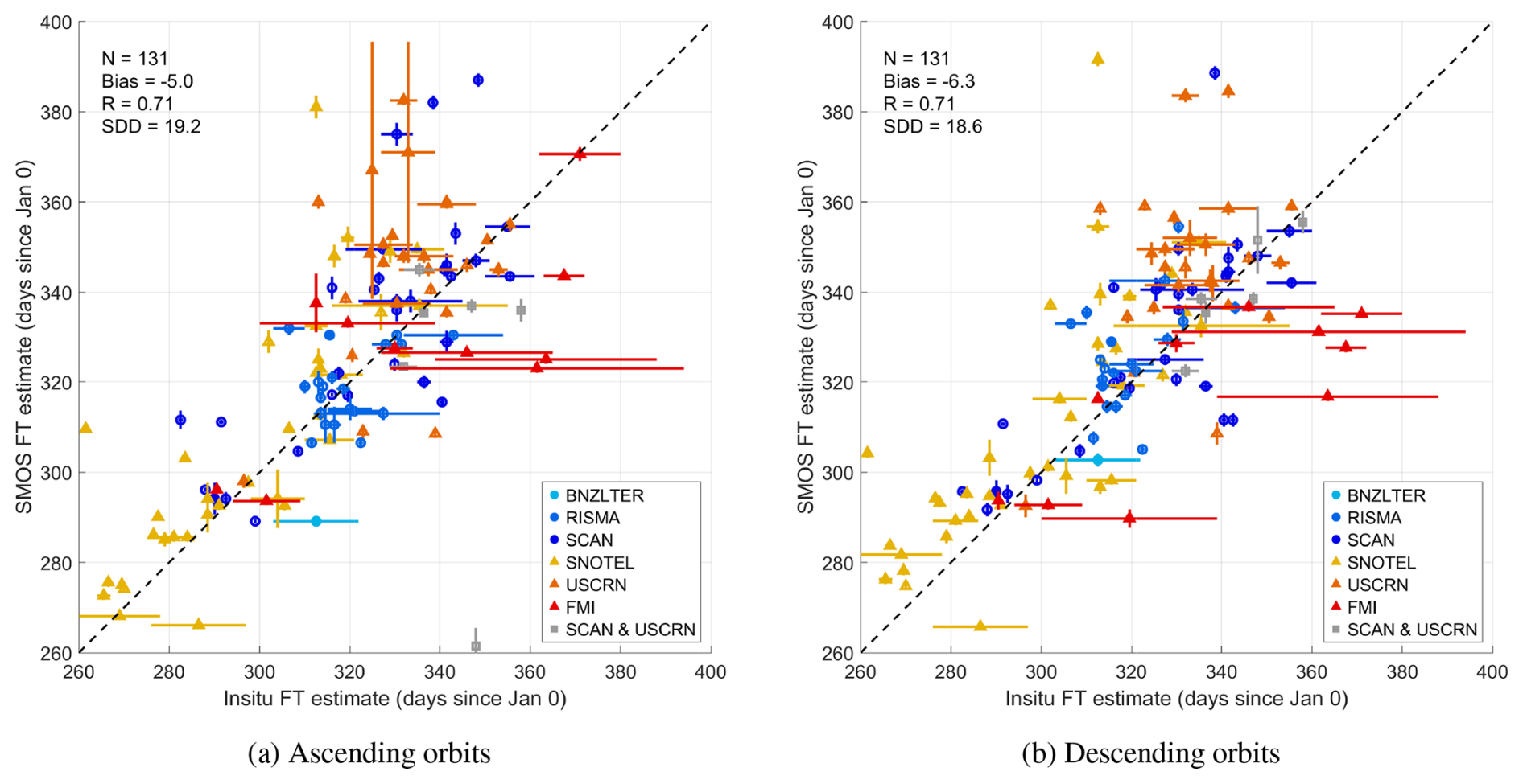
Figure 5 Comparison of the day of first freezing (DoFF) between SMOS L3FT and in situ data. (a) Horizontal axis: DoFF from the in situ data with the error bar derived from thresholds of 50 % to 90 %, with the marker set at the midpoint. Vertical axis: estimates from the SMOS ascending orbit data; the lower end of the error bar corresponds to DoFPF (day of first potential freezing), and the higher value corresponds to DoFF, with the marker set at the centre. (b) Same as (a) but for descending orbit data.

4.2 Comparison with ERA5-Land soil temperature data

We compared the SMOS FT with the ERA5-Land soil temperature (level 1 representing a depth of 0–7 cm) product to analyse their differences and compatibility. From the two products, SMOS is an observation-based product sensitive to the dielectric changes associated with soil freezing, while ERA5 is a model-based product representing the temperature of the soil. The two products were compared by deriving a day of first freezing (DoFF) from each dataset for each freezing period between 2010 and 2024.

Figure 6 shows maps of the average DoFF derived from SMOS FT ascending and descending orbits separately and from the ERA5 soil temperature product. SMOS FT and ERA5 show broadly similar DoFF patterns, particularly at high latitudes. However, discrepancies become more evident at lower latitudes, where SMOS has fewer observations and is more affected by RFI, especially in Eurasia. Differences also reflect expected latitudinal variation in the DoFF dynamics.

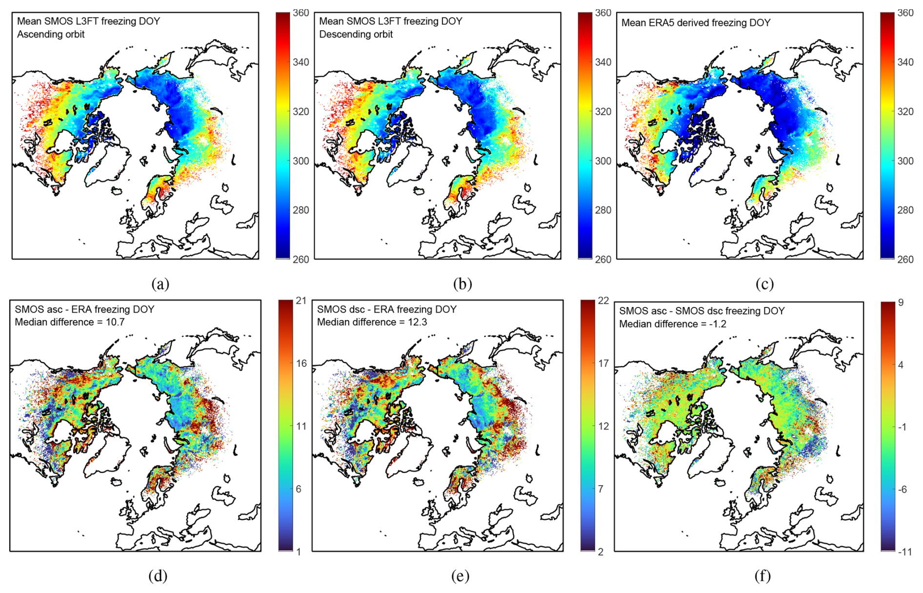
Figure 6 Average DoFF for the freezing periods between 2010 and 2024: (a) SMOS FT product with ascending orbits, (b) SMOS FT product with descending orbits, and (c) ERA5-Land soil layer 1 temperature-derived first freezing. Average values where the freezing day was successfully estimated from the data for 10 or more years are shown. The ERA5-derived mean freezing day is shown only for those values where also SMOS FT has a successful estimate. Panels (d)–(f) show the differences; note that the colour bars are centred around the global median of the differences to highlight the spatial variability of the differences.

To better highlight spatial differences, we introduce DoFF difference maps in Fig. 6d–f. These show SMOS ascending minus ERA5 (d), SMOS descending minus ERA5 (e), and SMOS ascending minus descending (f). All maps use a centred colour scale to emphasize spatial variability. The SMOS FT product tends to estimate later freezing compared to ERA5, with median differences of +10.7 and +12.3 d for ascending and descending overpasses, respectively. These differences are spatially heterogeneous. Notably, larger DoFF differences occur in regions with dense forest cover, particularly in boreal Eurasia and parts of North America, where increased vegetation canopy attenuates the L-band signal and amplifies NPR uncertainty; in regions affected by strong RFI, such as Eastern Europe and parts of Russia, where the SMOS observation density is lower and retrieval quality is reduced; and in mountainous or topographically complex terrain (e.g. Scandinavia, Alaska), where sub-grid heterogeneity can lead to mismatches between model-based and radiometric observations.

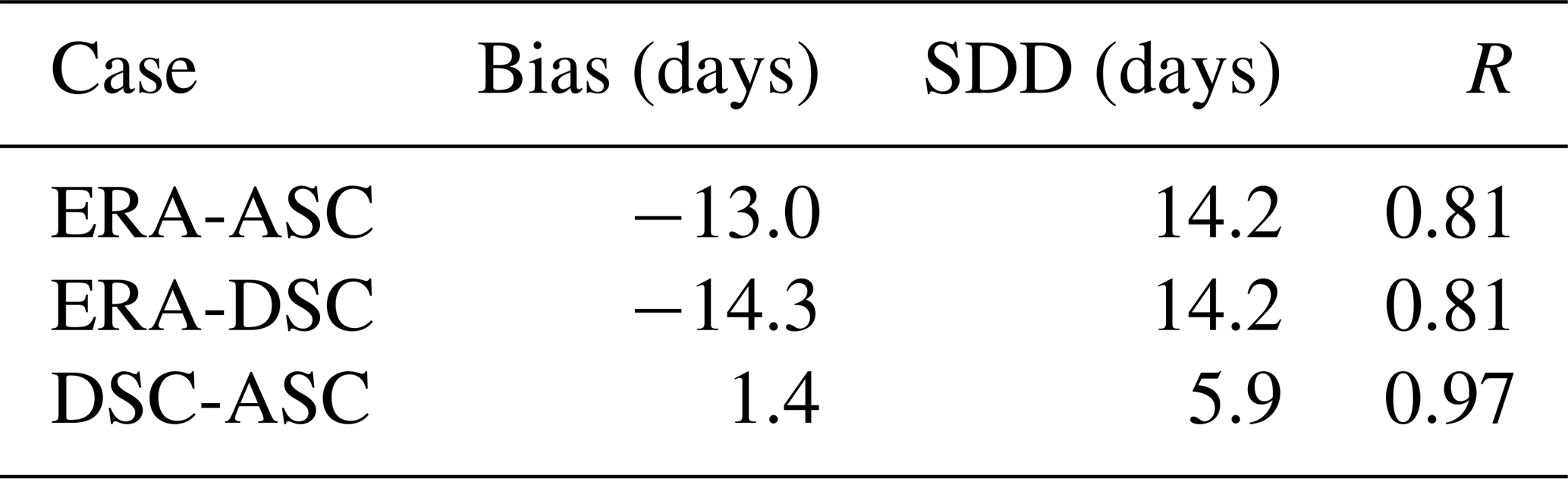
Figure 7 shows scatter plots comparing the mean days of first freezing between the datasets. The associated statistics are shown in Table 6. In general, SMOS seems to estimate later freezing than the ERA5 soil temperature would indicate (13–14 d on global average). Possible reasons for this difference include the following: (1) the SMOS observation frequency – it is possible that SMOS observes the freezing later simply due to delayed good quality observation with respect to the soil freezing. RFI is a usual disruption to the SMOS observations. (2) The estimation of the day of first freezing from the two datasets is slightly different, as the SMOS observation times have to be accounted for. (3) Systematic errors in the ERA5 soil temperature data – in particular, the first freezing is derived by looking at the time when the soil temperature drops below 0 °C. This estimate might be sensitive to errors in the modelled temperature values.

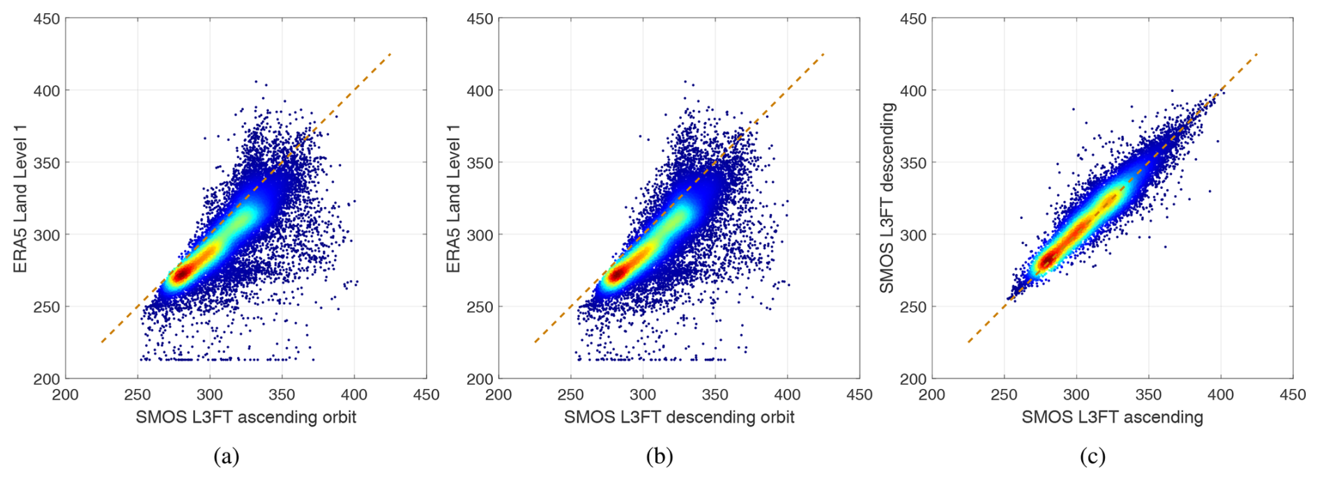
Figure 7 Scatter plots comparing the average DoFF between (a) SMOS FT ascending orbit and ERA5-Land-derived data, (b) SMOS FT descending orbit and ERA5-Land-derived data, and (c) SMOS FT ascending and descending orbits.

Table 6 Statistics corresponding to Fig. 7.

Furthermore, land cover distribution within the SMOS footprint affects the SMOS FT performance. High areal coverage of forest and water bodies, on the one hand, dampens the observed FT signal, making the freeze–thaw detection more difficult, and, on the other hand, creates their own contribution to the SMOS observation that are not fully accounted for in the SMOS FT product.

5 Product limitations

5.1 General limitations

The SMOS FT retrieval algorithm detects permittivity changes caused by the phase transition (or change in the aggregate state) of liquid soil water to ice. In regions with dry soils, this permittivity change is inherently small because the soil already has a low dielectric constant – even when unfrozen. As a result, the polarization contrast, and consequently the variability in the normalized polarization ratio (NPR), is limited. The low NPR dynamics reduces the sensitivity of the algorithm to freeze–thaw transitions in such environments. Also, areas with a very thin or non-existent soil layer (e.g. rocky areas and mountains) are challenging. At the L-band, the typical penetration depth ranges from a few centimetres to 10–15 cm, depending on the amount of free liquid water in the soil. Therefore, the detection of soil conditions based on L-band observations is limited to the near-surface layer, which is still significantly thicker compared to the surface layer detected by higher-frequency radiometers and optical sensors.

5.2 Spatial and temporal coverage

SMOS observations cover the entire globe twice in 3 d. The northernmost land areas have daily overflights due to the orbit configuration. Prior to the SMOS mission, passive L-band microwave observations were only made in space during the Skylab 3 mission in 1973 (Jackson and Eagleman, 2004). The revelation of the strong presence of man-made RFI in the protected frequency band (1400–1427 MHz) following the SMOS launch was a surprise (Oliva et al., 2012, 2016). As a consequence of the RFI level, spatial coverage over the Eurasian continent is severely hampered, moreover increasing significantly over Eastern Europe after 2022. Figure 8 shows the average observation interval (in days) of the SMOS FT product for the period 1 June 2010–31 December 2021 for ascending and descending orbits. The more frequent observations towards the north due to the orbit configuration are clearly visible. The presence of RFI increases towards the south on the Eurasian continent and primarily affects the descending orbit observations due to the forward tilt of the instrument. The North American continent is much less affected by RFI contamination, except for the first years of SMOS operation. Figure 9 shows the average observation interval (in days) for the period 1 January 2022 to 1 June 2024. The increased RFI contamination over Europe is clearly visible, hampering the SMOS FT product over a considerable area. While SMOS has provided valuable L-band observations since 2010, RFI, particularly over parts of Eurasia, remains a significant challenge for data continuity. The Soil Moisture Active Passive (SMAP) mission, launched in 2015, also operates in the L-band and incorporates onboard RFI detection and mitigation techniques that help reduce the impact of radio interference in some regions (Piepmeier et al., 2014). As such, SMAP can serve as a complementary source of L-band brightness temperature data for freeze–thaw applications, particularly in areas where SMOS data quality is frequently compromised.

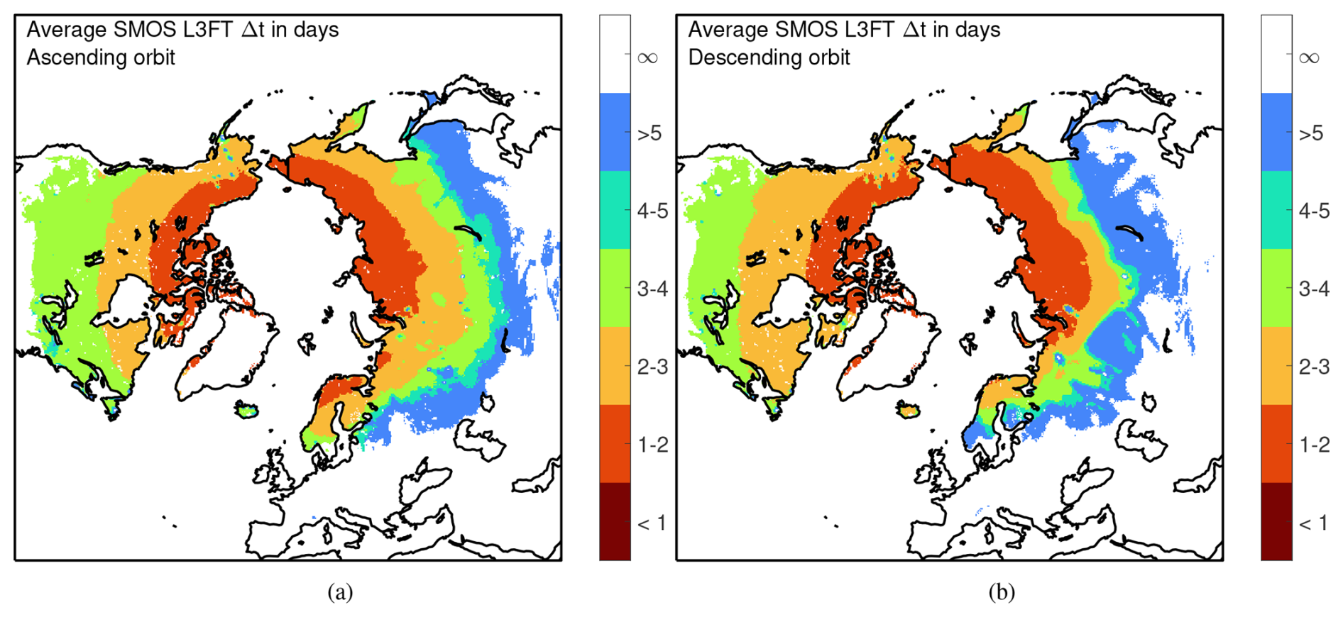
Figure 8 Average observation interval of the SMOS FT product, measured in days. The average is computed between 1 June 2010 and 31 December 2021 for (a) ascending and (b) descending orbits.

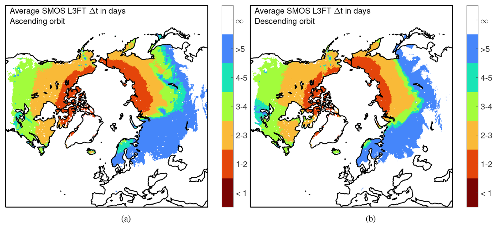
Figure 9 Same as Fig. 8 but for the time period 1 January 2022 to 1 June 2024.

An important feature of the SMOS FT product is that it contains data indicating the date of the last acquired observation for each location. This information is crucial for interpreting the data accurately, as it allows users to assess the timeliness of the observations. If the last observation was acquired several days before the release of the current product, there may be a significant gap in the data. During this period, changes in the soil state, such as a transition from thawed to frozen conditions, could have occurred at any point between the latest observation and the current product date. Users must be aware that large gaps in observation frequency can introduce uncertainty in the soil state estimates, making it essential to consult the last observation date when analysing the product data.

5.3 Wet snow

The presence of wet snow hampers the ability of SMOS L-band observations to detect soil conditions, particularly during spring. As snow begins to melt, its high liquid water content attenuates the microwave signal from the underlying soil and strongly affects the observed brightness temperatures, especially in horizontal polarization (Pellarin et al., 2016). This leads to increased polarization contrast and elevated values of the normalized polarization ratio (NPR), similar to those observed for thawed, moist soils. While snowmelt and soil thaw often occur concurrently in spring, the timing can vary, and the L-band signal cannot unambiguously distinguish between wet snow and actual thawed soil. Consequently, the SMOS FT algorithm may misinterpret the presence of wet snow as an early soil thaw, introducing uncertainty in the retrieval during the spring melt period. Variations in L-band brightness temperature in spring should thus rather be interpreted as information about the presence of liquid water in snow (Rautiainen and Holmberg, 2023). However, due to the partial penetration of L-band microwave radiation even in wet snow, the interpretation of the signal is less straightforward than at higher frequencies. On the other hand, this carries the potential to retrieve the liquid water content of snow (Houtz et al., 2021) and also the density of snow (Schwank et al., 2015; Lemmetyinen et al., 2016; Naderpour et al., 2017).

6 Data availability

The operational SMOS L3FT data record DOI is https://doi.org/10.57780/sm1-fbf89e0 (ESA, 2023). Data are available from the ESA SMOS online dissemination service (https://doi.org/10.57780/sm1-fbf89e0) and from the FMI dissemination service (https://litdb.fmi.fi/outgoing/SMOS-FTService/OperationalFT/, last access: 2 October 2025). The associated documentation, the algorithm theoretical baseline document, the product description document, and the read-me-first note are available from both services.

The input datasets used in this study are publicly available: CATDS L3TB brightness temperatures (Al Bitar et al., 2017, https://doi.org/10.12770/6294e08c-baec-4282-a251-33fee22ec67f), IMS Daily Northern Hemisphere Snow and Ice Analysis (U.S. National Ice Center, 2008, https://doi.org/10.7265/N52R3PMC), and ERA5-Land reanalysis (Muñoz Sabater, 2019, https://doi.org/10.24381/cds.e2161bac).

7 Conclusions

The SMOS FT product provides daily monitoring of the freeze–thaw (FT) state of Northern Hemisphere land surfaces at a spatial resolution of 25 km. The first operational SMOS FT product, made public in 2018, was developed from the prototype algorithm presented by Rautiainen et al. (2016). The updated SMOS FT product (version 3.01), presented here, offers a tool for monitoring seasonal freeze–thaw cycles, particularly across high-latitude regions. The L-band passive microwave observations used in this product are effective in detecting soil FT transitions due to the sensitivity of L-band brightness temperatures to changes in soil permittivity between frozen and thawed states.

The updated SMOS FT algorithm incorporates several improvements. These include enhanced noise removal through temporal filtering of the SMOS signal, which has improved the accuracy and reliability of the freeze–thaw detection. The validation of the SMOS FT estimates against in situ SM and ST data from the international soil moisture network, along with comparisons to the ERA5-Land reanalysis soil temperature data, demonstrates the product's robustness in identifying the day of first freezing in autumn, a critical parameter for greenhouse gas emissions studies.

However, certain limitations do remain. The SMOS FT product is less effective in regions with dry soils, thin soil layers, dense forested regions, or significant radio frequency interference (RFI), particularly in Eurasia. Additionally, the presence of wet snow in spring can obscure soil thawing detection, and variations in L-band signals during spring should be interpreted as an indication of wet snow rather than soil conditions; however, unambiguous detection of wet snow from the L-band is itself also more challenging than at higher frequencies due to partial penetration in wet snow. Furthermore, after the spring of 2022, the exceptionally strong presence of RFI over Eastern Europe has hindered the SMOS FT product over large areas.

In conclusion, while the SMOS FT product shows strong performance in high-latitude environments, future work should focus on addressing the limitations posed by RFI and wet snow layers. Continued refinement of the algorithm and further validation in different environmental conditions will enhance the product's utility for climate change studies, ecosystem monitoring, and land-use management.

Additionally, SMOS FT data have been utilized in the CarbonTracker Europe inverse modelling system at the Finnish Meteorological Institute to improve methane flux estimates at high latitudes. By aiding in the characterization of cold-season emissions, the integration of SMOS FT data has demonstrated its value in reducing uncertainties and supporting studies of methane dynamics in northern ecosystems (Erkkilä et al., 2023; Tenkanen et al., 2021).