CRA-LICOM: a global high-frequency atmospheric and oceanic temporal gravity field product (2002–2024)

Modeling sub-daily mass changes, dominated by the atmosphere and the oceans, is a fundamental requirement for nearly all existing terrestrial or space-borne geodetic observations to perform signal separation. Removing these high-frequency mass changes, through the usage of so-called de-aliasing products, is of particular interest for satellite gravity missions such as GRACE and GRACE-FO to prevent the aliasing of short-term mass changes into seasonal and long-term mass variability. Ongoing efforts focus on simulating this high-frequency signal by driving atmospheric/oceanic numerical models with specific climate-forcing fields and assimilating observational data. In this study, we establish China's first de-aliasing computation platform, achieved by using the recently released CRA-40 (China's first generation of atmospheric reanalysis) as forcing fields to drive our in-house 3-D atmospheric integration model and the LASG/IAP (State Key Laboratory of Numerical Modeling for Atmospheric Sciences and Geophysical Fluid Dynamics/Institute of Atmospheric Physics) Climate System Ocean Model 3.0 (LICOM3.0). With this new platform, we reproduce an alternative high-frequency atmospheric and oceanic gravity de-aliasing product, called CRA-LICOM, at 6 hourly and 50 km resolution, covering 2002–2024 at a global scale. The product is freely available at https://doi.org/10.11888/SolidEar.tpdc.302016 (Liu et al., 2025a). Inter-comparisons with the products of GFZ (Helmholtz Centre for Geosciences) and validations against independent observations reveal: (i) the current version of CRA-LICOM satisfies the requirement of the state-of-the-art satellite gravity missions, as well as other geodetic measurements, and (ii) despite agreement across most areas, considerable uncertainty is found at marginal seas near continental shelves, particularly at high-latitude regions. Therefore, scientific applications that aim to understand the sub-daily atmospheric-oceanic water exchange, as well as mission design of future satellite gravity that seeks accurate gravity de-aliasing, can use our product as a reliable source. Nevertheless, the current platform has the potential to be improved in terms of modeling and data assimilation capacity, which will be outlined in this study.

1 Introduction

Changes in Earth's gravity field reflect mass redistributions in surface fluids such as the atmosphere (A), ocean (O), hydrology (H), ice sheets (I) and solid Earth (S). Accurate disaggregation of the temporal gravity field into these sources is crucial to understanding the natural evolution of each process on and beneath the Earth (Wahr et al., 1998; Tapley et al., 2019). For example, Terrestrial Water Storage (TWS, associated with the H component) is considered an essential climate variable to diagnose the internal variability of the global water cycle and climate change (Rodell et al., 2018; Rodell and Reager, 2023).

In particular, state-of-the-art geodetic observations from, e.g., terrestrial/space-borne gravity (see Güntner et al., 2017) and GNSS (Global Navigation Satellite System, see White et al., 2022; Klos et al., 2023), often represent a mixture of these sources, that is, AOHIS (A + O + H + I + S), where separation is required to obtain desired components, such as TWS or HIS (H + I + S). Generally speaking, a reduction of AO (A + O) from the total signal is feasible because it is dominated by high-frequency changes, whereas TWS or HIS often associate with relatively slower gravity changes. Therefore, precise AO modeling is not only essential for understanding rapid climate changes but is also relevant as an a priori model to separate TWS or HIS from other signals.

In addition, the AO model is vital for the Gravity Recovery and Climate Experiment mission (GRACE, 2002–2017; Tapley et al., 2004) and its follow-on mission (GRACE-FO, 2018-present; Landerer et al., 2020), which provides monthly snapshots of HIS (when AO is perfectly removed) changes globally with unprecedented precision (Velicogna and Wahr, 2006; Scanlon et al., 2018; Chao and Liau, 2019). However, accurate acquisition of HIS components depends on reliable AO prior models to reduce aliasing errors (Wahr et al., 1998). Such errors significantly degrade HIS estimations because sub-daily AO variability is much below the feasible temporal resolution of GRACE (e.g., Han et al., 2004; Forootan et al., 2014). These aliasing errors are among the largest error sources in current space-borne gravity missions and may restrict next-generation missions (Han et al., 2007; Seo et al., 2008; Liu and Sneeuw, 2021; Chen et al., 2022), despite improved onboard instruments (Flechtner et al., 2016; Zhou et al., 2021), unless faster sampling strategies or co-estimations of AO parameters are applied (Kurtenbach et al., 2009; Wiese et al., 2011; Mayer-Gürr et al., 2012; Daras and Pail, 2017; Hauk and Pail, 2018; Mayer-Gürr et al., 2018; Purkhauser and Pail, 2019). In addition to GRACE(-FO), AO modeling is relevant to other geodetic techniques. For example, it improves the determination of the satellite altimetry orbit (Cerri et al., 2010; Rudenko et al., 2016; Bonin and Save, 2020) and is a mandatory post-processing step for terrestrial gravity measurements (Boy et al., 2002, 2009) and GNSS station displacement measurements (Dill and Dobslaw, 2013; Han and Razeghi, 2017; Swarr et al., 2024). Consequently, efforts to achieve precise AO modeling remain ongoing within the geodesy community.

Generally, the AO model consists of tidal and non-tidal constituents, whereas we shall use the term AO to mainly indicate the non-tidal high-frequency (sub-daily) aspect hereinafter to avoid confusion. Current AO models often use climate forcing fields, followed by atmospheric gravity calculation through vertical integration of air mass, and oceanic gravity simulation through ocean circulation models (Wahr et al., 1998). So far, the only publicly available AO model is maintained by GFZ, which has long been relied upon to produce monthly gravity fields by the major GRACE (-FO) data processing centers worldwide (Dobslaw et al., 2017; Shihora et al., 2022a). Their product has evolved substantially over the past two decades, focusing on improving atmospheric forcing fields (Duan et al., 2012; Hardy et al., 2017; Yang et al., 2021), refining atmospheric integration (Swenson and Wahr, 2002; Boy and Chao, 2005; Zenner et al., 2010; Forootan et al., 2013; Dobslaw et al., 2017), and switching forced ocean models (Bonin and Save, 2020; Schindelegger et al., 2021; Shihora et al., 2022a). Due to these efforts, their latest product, AOD1B-RL07 (called GFZ-RL07 hereinafter to avoid confusion), has reached a high-quality level. However, as addressed by Shihora et al. (2022a), GFZ-RL07 is inevitably imperfect in capturing the high-frequency variability, particularly the oceanic component, since it is a purely atmospherically forced oceanic simulation without constraints from observations.

Recognizing that there is still a considerable error in the AO model, it would be beneficial to increase the diversity of the AO model to better understand its uncertainty for further improvement (Springer et al., 2024), rather than having GFZ-RL07 as the only option, and this also builds the motivation for this work. In fact, GFZ-RL07 has long relied on atmospheric operational data or reanalysis from ECMWF (European Center for Medium-Range Weather Forecasts) as forcing data, and another available AO model produced by Gegout (2020) also relies on ECMWF data, and unfortunately has stopped updating from 2017. In this context, developing another AO model independent of the GFZ-RL07 model should expect to apply a completely different atmosphere forcing and oceanic model. In November 2013, the China Meteorological Administration (CMA) launched the global reanalysis project, and after ten years of effort, China's first generation global atmospheric and land reanalysis product (named CRA-40) became publicly available (Liu et al., 2023). Intensive evaluations of CRA-40 (see Shen et al., 2022; Liu et al., 2023) have shown a better performance than the existing global reanalysis products to the latest ECMWF reanalysis, particularly in terms of surface pressure, temperature, and specific humidity, etc., which are exactly the key variables used to establish the AO model. In addition to the new forcing dataset, we also introduce LICOM3.0 in-house, an advanced ocean model among the best peer models in the world (Lin et al., 2020), to simulate oceanic variables, including ocean bottom pressure (OBP) that reflects the oceanic mass/gravity change (Liu et al., 2012).

In this study, due to the release of CRA-40, in conjunction with the ocean model LICOM, it is possible for us to develop an up-to-date global high-frequency atmospheric and oceanic gravity product, named CRA-LICOM (2002–present), which is completely independent of GFZ-RL07. We anticipate that this alternative could diversify the gravity recovery options from GRACE(-FO), and provide an opportunity to access the AO full time-scale uncertainty via an inter-comparison between these two independent products (Shihora et al., 2024). It was revealed by Kvas and Mayer-Gürr (2019) that accounting for the AO uncertainty information in GRACE(-FO)'s gravity recovery would considerably enhance the quality, and this strategy is suggested as the standard processing chain for official producers as well.

In this paper, we first introduce the input data sets for both modeling and validation in Sect. 2. Subsequently, a brief description of the atmospheric/oceanic gravity modeling methodology is addressed in Sect. 3. Then, we demonstrate the main output of the CRA-LICOM products in Sect. 4 and evaluate their performance with independent observations in Sect. 5. Finally, we analyze the limitations of the current release of the CRA-LICOM product in Sect. 6, discuss the conclusions, and outline the way forward in Sect. 8.

2 Input dataset description

2.1 Modeling dataset

China's first-generation global atmospheric and land reanalysis, CRA-40, is chosen herein as the climate-forcing field. It applies to the National Centers for Environmental Prediction (NCEP) Global Spectral Model (GSM)/Gridpoint Statistical Interpolation (GSI) 3D-Var system at a 6 h time interval with 64 vertical levels spanning from surface to 0.27 hPa and a horizontal resolution of 34 km. A large number of reprocessed satellite datasets and widely collected conventional observations were assimilated during reanalysis, including reprocessed atmospheric motion vectors from FY-2C/D/E/G (Chinese Fengyun-2 geostationary satellites) satellites, dense conventional data over China, as well as MWHS-2 and GNSS-RO observations from FY-3C (CMA's Fengyun-3 polar orbiting satellite, Jiang et al., 2020). The original model-level output is post-processed into 47 pressure levels, and then all variables are interpolated to four horizontal resolutions in longitude–latitude projection, including 0.25, 0.5, 1 and 2.5°. CRA-40 can be accessed via http://data.cma.cn/CRA (last access: 14 June 2024), where, for our study, the dataset covering 2000–2024 is extracted. To balance accuracy and computational efficiency, the spatial/temporal resolution, i.e., 0.5°/6 h of CRA-40, is selected for all variables required in this study. A higher spatial resolution, such as 0.25°, is not considered currently since GRACE's resolution is much coarser, e.g., 3° (Landerer and Swenson, 2012). Specifically, four variables are required to facilitate the atmospheric gravity field modeling, which are the surface pressure, the surface geopotential, the multi-layered temperature (pressure level), and the multi-layered specific humidity (pressure level). On the other hand, 11 variables are required to force the LICOM3.0 model, which are air density, temperature, zonal wind speed, meridional wind speed, specific humidity at 10 m, sea surface pressure, runoff, precipitation, downward long-wave radiation flux, downward shortwave radiation flux, and upward shortwave radiation flux.

2.2 Validation dataset

2.2.1 GFZ-RL07 AO model

The GFZ-RL07 AO model is the official de-aliasing product for all existing satellite gravity missions. It consists of an atmospheric component based on operational and reanalysis (ERA5; Hersbach et al., 2020) datasets of the ECMWF, and an oceanic component derived from unconstrained simulations using the MPIOM (Max Planck Institute for Meteorology Ocean Model; Jungclaus et al., 2013) ocean model, which is consistently forced by the corresponding atmospheric fields of the ECMWF. Unlike CRA-40, ERA5 is based on the Integrated Forecasting System (IFS) Cycle 41r2 with 4D-Var data assimilation, which provides hourly output at 31 km horizontal resolution and includes 137 vertical levels up to 0.01 hPa. The data assimilation system utilizes observations from more than 200 satellite instruments and conventional sources, including selected data from FY-3B/C (Chen et al., 2014; Lawrence et al., 2018). MPIOM uses a 1° tri-polar Arakawa-C grid with 40 vertical levels and newly includes cavities underneath the Antarctic ice-shelf and SAL (self-attraction and loading; Ray, 1998; Shihora et al., 2022b) feedback. GFZ RL07 AO model provides non-tidal atmospheric and oceanic components with 3 h temporal resolution and spherical harmonic expansion up to degree/order 180 alongside selected tidal constituents slower than 6 h. GFZ-RL07 is accessible via https://isdc.gfz-potsdam.de/esmdata/aod1b/ (last access: 29 March 2024) and is used here for comparison with CRA-LICOM.

2.2.2 GRACE Level-1b and Level-2 data

Temporal gravity field (Level-2) using GRACE Level-1b products can be used to assess the accuracy of CRA-LICOM for current satellite gravity missions. GRACE Level-1b products, including along-track range(-rate), accelerometer, star camera attitude, and reduced dynamic orbit data, are available at https://podaac.jpl.nasa.gov/dataset/GRACE_L1B_GRAV_JPL_RL03 (last access: 20 December 2024). Additionally, the latest version (RL06) of GRACE Level-2 temporal gravity fields (in terms of spherical harmonic coefficient) from CSR (Center for Space Research from the University of Texas at Austin, Texas, USA), JPL (Jet Propulsion Laboratory, USA), and GFZ are used for further validation, accessible via https://icgem.gfz-potsdam.de/home (last access: 5 January 2025).

2.2.3 Altimeter and Argo

Altimeter is widely used to monitor sea level change that consists of the steric and non-steric compartments, where the latter is mainly caused by mass change. As Argo is capable of measuring the steric sea level, the altimeter combined with Argo can reflect the non-steric sea level, theoretically equivalent to GRACE-derived ocean mass change plus the currents, that is, the AO model (Gregory et al., 2019). Therefore, Altimeter and Argo are often used to validate GRACE as well as its underlying AO model (Chen et al., 2018). In this study, an ensemble of three Argo products is adopted, that is, BOA (Li et al., 2017), EN4 (Good et al., 2013), and SIO (Roemmich and Gilson, 2009), covering the upper ocean above 2000 m. Altimeter data are collected from AVISO at a resolution of 0.25° × 0.25° and 10 d intervals, with further calibration of GIA (Glacier Isostatic Adjustment, see Caron et al., 2018) as suggested.

2.2.4 OBP Recorders and related variables from Argo

Ocean Bottom Pressure (OBP) data from the Deep Ocean Assessment and Reporting of Tsunamis (DART) system (National Oceanic and Atmospheric Administration, 2005) are utilized for validation. We download the quality-controlled and de-tided OBP data (Mungov et al., 2013) with a 15 s resolution from DART for the period 2002–2018. After processing the OBP into hourly mean data, we select timestamps every six hours starting from 00:00, such as 00:00, 06:00 (UTC 00:00), and so on. Finally, we obtained OBP datasets that included 68 locations between the years 2002 and 2023, mainly distributed over the Pacific and Atlantic Oceans. In addition, the global temperature and salinity obtained from Argo are used to further validate the simulated oceanic conditions, which are critical for accurate OBP simulations. Such monthly Argo data span 2005–2020 with a horizontal resolution of 1° × 1° and a vertical resolution of 27 layers (depths of up to 2000 m), which are available at https://apdrc.soest.hawaii.edu/projects/Argo/data/gridded/On_standard_levels/index-1.html (last access: 14 December 2024).

2.2.5 GLDAS

The additional data set includes GLDAS (Global Land Data Assimilation System, https://ldas.gsfc.nasa.gov/gldas/, last access: 1 February 2025), which is based on advanced land surface modeling and data assimilation techniques to merge satellite- and ground-based observations into the model. GLDAS provides high-quality global land surface fields to support the investigation of change in TWS (Li et al., 2019). In this study, we extract TWS (3 h and 1° × 1°) from GLDAS to approximate the component of the global hydrology (H) signal to be compared with the AO component, as indicated by CRA-LICOM.

3 Method

In summary, the process to obtain CRA-LICOM products consists of three major steps: (i) atmospheric gravity field modeling, (ii) oceanic gravity field modeling, and (iii) post-processing to produce the final CRA-LICOM, see Fig. 1 for a conceptual diagram of the framework. In what follows, the specific method in each step is addressed individually.

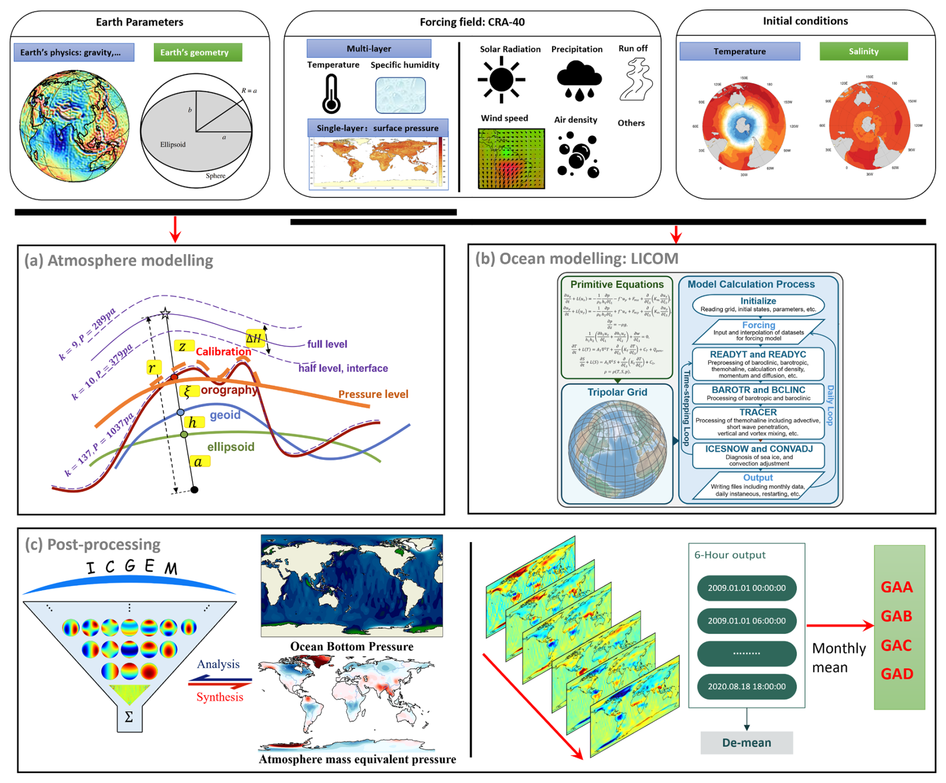
Figure 1 The diagram to illustrate the workflow of CRA-LICOM: from the input forcing field (associated with auxiliary parameters) to the output gravity products, where three major steps are addressed: (a) atmospheric gravity field modeling to calculate the surface mass and upper air mass contribution to the gravity field, using calibrated pressure level data, (b) oceanic gravity field modeling with LICOM to simulate the ocean bottom pressure forced by the atmospheric variables from CRA40, (c) post-processing of the grid output to the spherical harmonic coefficients, the removal of long-term mean, and the aggregation of monthly products.

3.1 Atmosphere

3.1.1 Atmospheric tidal constituents

The input surface pressure fields represent a mixture of tidal and non-tidal constituents, which should be isolated as a first step. The logic behind the isolation is the fact that the model can often better predict tides. As limited by Nyquist sampling law, the expected tidal signals extracted from CRA-40 (6 hourly) must be slower than the semi-diurnal tide, which includes P₁ (14.9589314° h⁻¹), S₁ (15.0000000° h⁻¹), K₁ (15.0410686° h⁻¹), N₂ (28.4397295° h⁻¹), M₂ (28.9841042° h⁻¹), L₂ (29.5284789 deg/h) and T₂ (29.9589333° h⁻¹). Then, a point-wise tidal pressure can be obtained from a summation of all these frequency-dependent tides ζ_s (assuming a tide s with frequency ω_s, amplitude ξ_s and phase δ_s) following

$$\begin{array}{}\text{(1)}& \begin{array}{rl}\mathit{\zeta }(\mathit{\theta },\mathit{\lambda },t)& =\sum _s{\mathit{\xi }}_s(\mathit{\theta },\mathit{\lambda })\cos [{\mathit{\omega }}_{s}t+{\mathit{\chi }}_s-{\mathit{\delta }}_s(\mathit{\theta },\mathit{\lambda }\left)\right]\\ & =\sum _s\left[A_s\right(\mathit{\theta },\mathit{\lambda }\left)\cos \right({\mathit{\omega }}_{s}t)+B_s(\mathit{\theta },\mathit{\lambda }\left)\sin \right({\mathit{\omega }}_{s}t\left)\right],\end{array}\end{array}$$

where (θ,λ) denotes the spherical coordinate (colatitude, longitude) of the point and t denotes an arbitrary time epoch. In particular, χ_s is the Warburg phase correction documented in Petit et al. (2010); the time reference where δ_s=0 is selected as 1 January 2007 00:00:00. And in Eq. (1) the amplitude and phase can be translated into the coefficients A_s(θ,λ) and B_s(θ,λ) to enable the ordinary least squares (OLS) solution. In this study, the OLS is configured by terms of trending C(θ,λ), tidal ζ(θ,λ) and non-tidal D(θ,λ) signals:

$$\begin{array}{}\text{(2)}& \begin{array}{rl}P(\mathit{\theta },\mathit{\lambda },t)& =\sum _s\left[A_s\right(\mathit{\theta },\mathit{\lambda }\left)\cos \right({\mathit{\omega }}_{s}t)+B_s(\mathit{\theta },\mathit{\lambda }\left)\sin \right({\mathit{\omega }}_{s}t\left)\right]\\ & +C(\mathit{\theta },\mathit{\lambda })t+D(\mathit{\theta },\mathit{\lambda }),\end{array}\end{array}$$

where parameters ($A_s,B_s,C,D$) are fitted from the “observations”, i.e., the time series of surface pressure $P(\mathit{\theta },\mathit{\lambda },t)$. Subsequently, each tide ζ_s (its amplitude and phase) can be recovered from its coefficients (A_s,B_s) via Eq. (1). Be aware that a high-pass filter (with a time window of 3 days) is applied to P beforehand, to damp non-tidal signals first and stabilize the tidal estimations. Here, the tide constituents are fitted from the years 2007–2014, consistent with the period used in AOD1B RL06 (Dobslaw et al., 2016).

3.1.2 Non-tidal air mass integration

To accurately reflect the non-tidal atmospheric gravity field change, one has to exploit layered observations to account for contributions from both surface and upper air anomalies. To this end, two types of air mass integration are required: (1) a surface integration that considers the air mass as a thin layer, that is, by neglecting the vertical structure of air; (2) a 3-D vertical integration of all mass columns to obtain the upper air contribution. Regardless of either type of integration, the first step is to obtain the “inner integral”, i.e., I_n, which is often degree dependent (the degree of spherical harmonic expansion); see Forootan et al. (2013, 2014). For surface integration, I_n is treated as

$$\begin{array}{}\text{(3)}& \begin{array}{rl}{I}_n^s(r,\mathit{\theta },\mathit{\lambda })& ={\left({\displaystyle \frac{r}{a_{\mathrm{e}}}}\right)}^{n+\mathrm{2}}{\displaystyle \frac{\mathrm{\Delta }{P}_{\mathrm{0}}(r,\mathit{\theta },\mathit{\lambda })}{g(r,\mathit{\theta },\mathit{\lambda })}}\\ & ={\left({\displaystyle \frac{a(\mathit{\theta },\mathit{\lambda })+\mathit{\zeta }(\mathit{\theta },\mathit{\lambda })+h(\mathit{\theta },\mathit{\lambda })}{a_{\mathrm{e}}}}\right)}^{n+\mathrm{2}}\\ & \cdot {\displaystyle \frac{\mathrm{\Delta }{P}_{\mathrm{0}}(r,\mathit{\theta },\mathit{\lambda })}{g(r,\mathit{\theta },\mathit{\lambda })}},\end{array}\end{array}$$

where $(r,\mathit{\theta },\mathit{\lambda })$ is the spherical coordinate (radial distance, colatitude, and longitude) of the evaluated point. In the case of a realistic Earth, the radial distance r consists of the ellipsoidal radius a, the geoid undulation h , and the topography ζ (e.g., Yang et al., 2022). In addition, in Eq. (3) a_e denotes the Earth's mean radius, e.g., ∼ 6 378 136.6 km; $g(r,\mathit{\theta },\mathit{\lambda })$ is the gravity acceleration of the evaluated point. $\mathrm{\Delta }{P}_{\mathrm{0}}(r,\mathit{\theta },\mathit{\lambda })$ indicates the pressure difference between two layers, but because only the surface layer is adopted here so that $\mathrm{\Delta }{P}_{\mathrm{0}}(r,\mathit{\theta },\mathit{\lambda })$ equals the surface pressure.

By contrast, the 3-D vertical integration is able to consider the vertical structure of the atmosphere by taking advantage of multi-level atmospheric input fields. Here, CRA-40, in terms of pressure levels, is used that yields

$$\begin{array}{}\text{(4)}& \begin{array}{rl}{I}_n^v(r,\mathit{\theta },\mathit{\lambda })& =\sum _{k=\mathrm{0}}^{k_{max}}({\displaystyle \frac{a(\mathit{\theta },\mathit{\lambda })+\mathit{\zeta }(\mathit{\theta },\mathit{\lambda })+h(\mathit{\theta },\mathit{\lambda })+z_k(\mathit{\theta },\mathit{\lambda })}{a_{\mathrm{e}}}}{)}^{n+\mathrm{2}}\\ & \cdot {\displaystyle \frac{\mathrm{\Delta }{P}_k(\mathit{\theta },\mathit{\lambda },r_k)}{g_k(\mathit{\theta },\mathit{\lambda },r_k)}},\end{array}\end{array}$$

where the inner integral is discretized into k-layers, and for CRA-40, it has maximal $k_{max}=\mathrm{47}$ layers. $\mathrm{\Delta }{P}_k(\mathit{\theta },\mathit{\lambda },r_k)$ indicates pressure difference between adjacent layers kth and (k−1)th. Comparing Eq. (4) to Eq. (3), the z_k emerges as the geometric distance from the evaluated point to the surface, which must be solved from an accumulation of geopotential differences between adjacent pressure layers. To this end, the multi-level humidity and temperature fields are required to obtain the geopotential height difference; see Boy and Chao (2005) for more details.

It is worth mentioning that because CRA-40 is given in terms of pressure level, integration with Eq. (4) might face risks of “outliers”: there could be some cases in which the pressure of a layer is greater than the surface pressure. In other words, the specific isobaric surface goes through the interior of the Earth, which is obviously unreasonable in physics. It is relevant to calibrate this outlier. Otherwise, the modeling quality would be significantly degraded. To this end, we propose a calibration method, which yields

$$\begin{array}{}\text{(5)}& V_k(\mathit{\theta },\mathit{\lambda })=V_{k-\mathrm{1}}(\mathit{\theta },\mathit{\lambda }),\forall \mathrm{\Delta }{P}_k(\mathit{\theta },\mathit{\lambda },r_k)<\mathrm{0},\end{array}$$

where V_k indicates an arbitrary variable in the kth layer, which could be either pressure, temperature, or humidity. In this manner, outliers can be identified and fixed with a reasonable approximation (the neighboring value at the next pressure level aloft). One can see our preliminary work (Zhang et al., 2025) for more details on the calibration approach for atmospheric pressure-level reanalysis, while this study will focus on the evaluation and validation of the AO model.

3.1.3 Non-tidal atmospheric correction

An accurate modeling of the non-tidal atmospheric gravity field requires us to account for both the direct gravitational effect and the indirect Earth's deformation effect. Therefore, a combination of the hypothetical thin-layered air (with two further corrections) and the upper air is necessary. The implementation of the combination follows the method proposed by Yang et al. (2021), i.e.,

$$\begin{array}{}\text{(6)}& I_n=(I_n^s-I_n^{\mathrm{tide}}+I_n^{\mathrm{IB}})+{\displaystyle \frac{\mathrm{1}}{\mathrm{1}+k_n}}(I_n^v-I_n^s),\end{array}$$

where the k_n indicates the degree-dependent load Love number, and the quantity in the first bracket indicates the non-tidal surface air that accounts for both the direct and indirect effects. By contrast, the other quantity in the second bracket indicates the upper air that accounts for only the direct effect, which makes sense since it cannot lead to Earth's deformation. In addition, corrections are made to the surface integral that includes: (i) tide removal as indicated by $I_n^{\mathrm{tide}}$, which can be modeled by Eq. (1), and (ii) Inverted Barometer (IB) correction as indicated by $I_n^{\mathrm{IB}}$, which is introduced to only include the static contribution to OBP into the ATM coefficients; please see Dobslaw et al. (2017) for more details.

3.2 Ocean

3.2.1 OBP simulation with LICOM3.0

We used the low-resolution global configuration of LICOM3.0 (Lin et al., 2020; Liu et al., 2012) to obtain 3 hourly, 360 × 218 tri-polar (equivalent to 1° on average) OBP data spanning 2002–2024, as depicted in Fig. 1b. The ocean model adopts primitive equations, comprising the full form of Navier-Stokes equations, continuity equations, conservation equations for temperature and salinity, and the equation of state for seawater. These equations are discretized on a tri-polar grid and 30 vertical layers. The model workflow consists of three main blocks:

1. Initialize: This block manages the reading of grids, initial states, and parameters. The initial conditions use global climatology for temperature and salinity from PHC3.0 (Polar Science Center Hydrographic Climatology; Steele et al., 2001)

2. Forcing and Output: This block inputs the forcing fields and outputs simulated data. The atmospheric forcing fields of the model are transformed from the 6 hourly 0.5° resolution variables in CRA-40 by applying the standard air-sea flux calculation methods of the Ocean Model Inter-comparison Project (Griffies et al., 2016; Large and Yeager, 2004).

3. Time-Stepping Kernels: This block contains the kernels for solving equations within the time loop. “READYT and READYC” computes terms in the barotropic and baroclinic equations. “BAROTR and BCLINIC” solve barotropic and baroclinic equations, while “TRACER” handles temperature and salinity equations. Furthermore, “ICESNOW and CONVADJ” deals with sea ice and deep convection in high-latitude regions (Wang et al., 2021).

More information on LICOM3.0 can be found in the Appendix A. In this paper, the model was spun up for five cycles from 2002–2023. Then, at the end of the 5th cycle, an integration from 1 January 2002, to existing months in 2024 was conducted and analyzed. LICOM reached equilibrium within six spin-up cycles (see Fig. A1 in Appendix A), suggesting that no artificial drift remains in the system. The OBP in LICOM3.0 is the sum of atmospheric pressure and the vertical integration of seawater density between dynamic sea level and ocean bottom, computed as

$$\begin{array}{}\text{(7)}& P_{\mathrm{b}}=P_{\mathrm{a}}+H_{\mathrm{0}}\mathit{\rho }\left(\mathrm{1}\right)g+\sum _{k=\mathrm{1}}^{\mathrm{30}}\mathit{\rho }\left(k\right)\mathrm{\Delta }z\left(k\right)g,\end{array}$$

where P_b is the OBP, P_a is atmospheric pressure, H₀ is dynamic sea level, ρ and ρ(1) are seawater density and its value at surface level, g (= 9.80665 m s⁻²) is the gravity acceleration, k is vertical layer number, and Δz is vertical layer thickness. Note that although Eq. (7) is applied in 3D at time t and position (θ,λ), the dimension notation is omitted for readability.

3.2.2 Oceanic tidal constituents

For the same reason as atmospheric gravity field modeling, ocean tides must be estimated and removed from the oceanic contribution to OBP. Be aware that LICOM3.0 does not directly simulate the lunisolar gravitational tides in the oceans. Hence, oceanic tidal fluctuations are solely induced by periodically varying atmospheric forcing. Furthermore, because atmospheric pressure is set to zero in the model's momentum equations, the resulting oceanic tides are mainly driven by tidal variations in other atmospheric forcings, such as solar radiation (e.g., Hagan, 1996; Hagan and Forbes, 2002, 2003) and wind (e.g., Morton et al., 1993; Avery et al., 1989), rather than barometric pressure loading. Therefore, the amplitudes and fluctuations of the simulated oceanic tides are likely much weaker than in reality. For example, the global mean amplitude of S₂ simulated by LICOM3.0 in this study is approximately 10¹ Pa, compared to ∼10³ Pa in the tidal models of Huang et al. (2024).

In addition to the seven tidal constituents mentioned in Sect. 3.1.1, S₂ (30.0000000° h⁻¹), R₂ (30.0410667° h⁻¹) and SK₃ (45.0410760° h⁻¹) are also removed using the T_TIDE package (Pawlowicz et al., 2002), due to a higher sampling rate of OBP, i.e., 3 h. In this study, tide fluctuations are calculated annually for 2002–2023. Furthermore, be aware that the effect of atmospheric loading must be removed beforehand. Hence, the overall formula to obtain non-tidal oceanic contribution to OBP follows

$$\begin{array}{}\text{(8)}& P_{\mathrm{b}}^{\mathrm{nt}}=(P_{\mathrm{b}}-P_{\mathrm{a}})-\mathrm{tide}(P_{\mathrm{b}}-P_{\mathrm{a}}),\end{array}$$

where $P_{\mathrm{b}}^{\mathrm{nt}}$ is the non-tidal oceanic contribution to OBP, and the second term indicates the removal of tides.

3.2.3 Non-tidal OBP correction

Because of the Boussinesq approximation in the momentum equations of LICOM, mass conservation is no longer preserved, as density changes within this volume-conservative model. To ensure mass conservation, a global mass correction has to be implemented following the method proposed by Greatbatch (1994). This correction involves subtracting the mean OBP across the entire ocean domain at each time step, which yields

$$\begin{array}{}\text{(9)}& P_{\mathrm{b}}^{\mathrm{dyn}}=P_{\mathrm{b}}^{\mathrm{nt}}-\mathrm{1}/A_{\mathrm{oceans}}\int P_{\mathrm{b}}^{\mathrm{nt}}\mathrm{d}A,\end{array}$$

where $P_{\mathrm{b}}^{\mathrm{dyn}}$ is the non-tidal dynamic OBP, which will be used in Eq. (3) as well to obtain the inner integral $I_n^{\mathrm{O}}$ of the ocean in Eq. (6). Be aware that the ultimate temporal resolution of $P_{\mathrm{b}}^{\mathrm{dyn}}$ is down-sampled from native 3 to 6 h to be consistent with that of the atmospheric forcing field.

3.3 Post-processing to CRA-LICOM

Having obtained the degree-dependent inner integral of the atmospheric ($I_n^{\mathrm{A}}$) and oceanic ($I_n^{\mathrm{O}}$) components, a harmonic analysis that maps the global multi-level gridded pressure fields ($I_n=I_n^{\mathrm{A}}+I_n^{\mathrm{O}}$) to the gravity field is necessary, which yields

$$\begin{array}{}\text{(10)}& \begin{array}{rl}{C}_{nm}+i{S}_{nm}& ={\displaystyle \frac{\mathrm{3}}{\mathrm{4}\mathit{\pi }{\mathit{\rho }}_{\mathrm{e}}}}{\displaystyle \frac{\mathrm{1}+k_n}{\mathrm{2}n+\mathrm{1}}}\underset{\mathrm{0}}{\overset{\mathrm{2}\mathit{\pi }}{\int }}\underset{\mathrm{0}}{\overset{\mathit{\pi }}{\int }}{I}_n\\ & \cdot P_{nm}\left(\cos \mathit{\theta }\right)e^{im\mathit{\lambda }}\sin \mathit{\theta }\mathrm{d}\mathit{\theta }\mathrm{d}\mathit{\lambda },\end{array}\end{array}$$

where P_nm(cos θ)e^imλ denotes the normalized surface spherical harmonics, k_n is the load Love number, and ρ_e is the Earth mean density, 5517 kg m⁻³; [C_nm,S_nm] are the corresponding coefficients of spherical harmonic expansion at degree n and order m. Solving [C_nm,S_nm] from Eq. (10) relies on a two-step procedure following Sneeuw (1994), but is implemented in practice degree by degree due to the degree-dependent nature of I_n. In addition, a long-term mean from 2003–2014 is subtracted from the time series, and the derived anomaly ΔI_n instead of I_n is applied to Eq. (10) eventually.

To be consistent with the de-aliasing conventions and nomenclature (Dobslaw et al., 2017), CRA-LICOM is further classified into four 6 h products: ATM (indicating only the non-tidal high-frequency atmospheric gravity field), OCN (indicating only the non-tidal high-frequency oceanic gravity field), GLO (the sum of ATM and OCN) and OBP (indicating only the ocean bottom pressure, and thus excluding the upper air contribution). Eventually, these four 6 h products are correspondingly post-processed into monthly mean products (ATM → GAA, OCN → GAB, GLO → GAC, OBP → GAD) for scientific users who are only concerned with the low-frequency phenomena. All of these constitute our final CRA-LICOM product, but “CRA-LICOM” hereafter always indicates the “GLO” product for simplicity, unless stated otherwise.

4 Results

4.1 Standard product

CRA-LICOM produces a high-frequency (6 hourly) global gravity field product with a spectral resolution of degree/order 180, which is finer than the wavelengths resolved by the GRACE and GRACE-FO missions (∼ 300 km or degree/order 60, see Landerer and Swenson, 2012). The product spans 2002 to 2024, and future updates will extend its coverage beyond 2024.

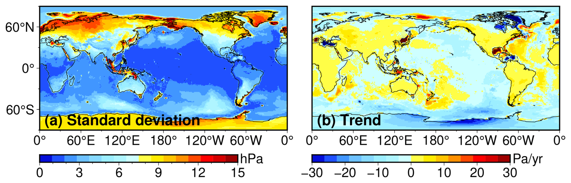
Figure 2 Equivalent pressure fields synthesized from CRA-LICOM during 2002–present: (a) the standard deviation (hPa), (b) the secular trend (Pa yr⁻¹).

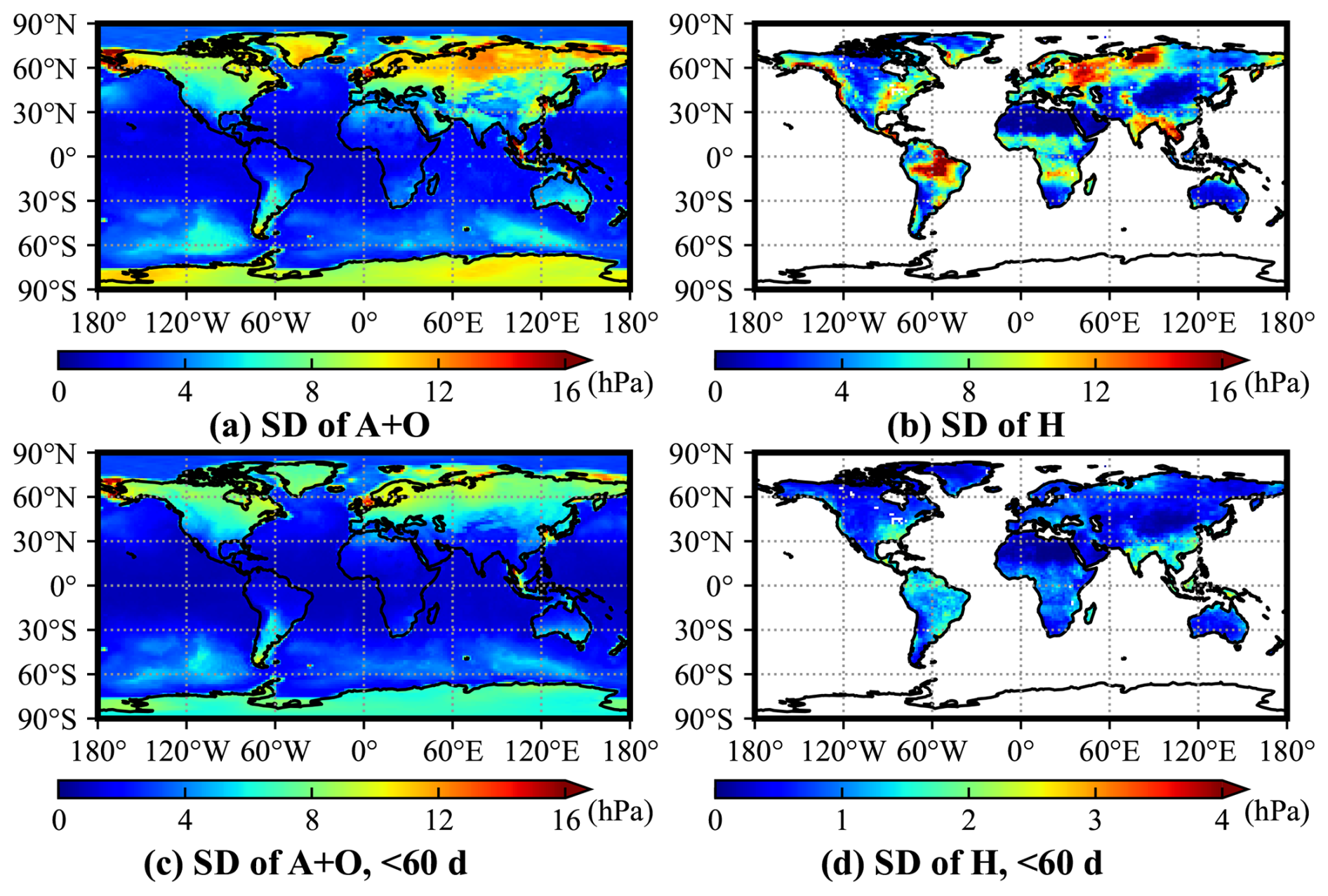
Figure 3 Comparison between AO and H variation of one year (2005). Panels (a)–(b) are SD of an entire year, while (c)–(d) are SD after Butterworth high-pass filtering with a 60 d cutoff window.

The standard deviation (SD) and secular trend of the product are illustrated in Fig. 2. The global mean SD is 4.72 hPa, comparable to GFZ-RL07 (4.98 hPa, see Fig. B1 of Appendix B). Variations are higher over continents (mean SD: 7.38 hPa) than over oceans (mean SD: 2.95 hPa), suggesting a dominant contribution from atmospheric mass changes over land. This is reasonable, as fast atmospheric mass changes over the open ocean are compensated by the IB response, leaving only the static contribution of surface atmospheric pressure. The secular trend shows a maximum of 108.13 Pa yr⁻¹ and a minimum of −78.92 Pa yr⁻¹ at a confidence level 95 %. Obviously, these trends contribute minimally to the overall signal, comparing Fig. 2a to b. However, areas with significant trends in Fig. 2b warrant cautious interpretation, particularly for GRACE(-FO) gravity fields obtained with CRA-LICOM. However, a majority (88.9 %) of the trend map is still within the range of ±10 Pa yr⁻¹, equivalent to ∼1 mm of change in water per year. For these areas, the CRA-LICOM trend could be considered as uncertainty since the AO product is not supposed to contain a trend by definition. However, this uncertainty is negligible considering that the GRACE (-FO) error can reach a few centimeters (Yang et al., 2024a). Nevertheless, this might be worth considering for next-generation gravity missions that target an accuracy of a few millimeters.

To understand the contribution of AO (CRA-LICOM) to Earth's gravity fields, we compared it against hydrology (H) variability using GLDAS-TWS data. The hourly GLDAS-TWS is down-sampled to 6 h to be consistent with AO. The experiment is carried out over 12 consecutive months (January 2005–December 2005, arbitrarily chosen), where the SD of one year of both AO and H are calculated, see Fig. 3a–b. It is found that A has a mean SD of 6.65 hPa (over the continents), O's mean SD is 4.27 hPa (over the oceans), and H's mean SD is 5.76 hPa (over the continents). Despite an overall comparable magnitude, much more pronounced variations can be captured from H than A over the climate zones, e.g., the Amazon and Ganges Delta. Then, we introduce high-pass filtering (Butterworth filtering) with a 60 d cut-off window to the one-year time series to retain only the high-frequency signals within the aliasing spectrum (twice the sampling rate of monthly gravity solution from GRACE(-FO)); see Fig. 3c–d. In this case, the AO component is much larger than H, that is, the mean SD of AO and H are 3.71 and 0.76 hPa, respectively. And AO has higher magnitudes compared to H in 94.2 % of continental areas. This confirms the necessity of incorporating AO in studies focusing on high-frequency gravity changes.

4.2 Auxiliary product

CRA-LICOM also provides auxiliary products, including tidal constituents and upper air anomalies. As primary tides, the solar diurnal tide S₁ and the lunar semi-diurnal tide M₂ in the atmosphere are shown in Fig. 4a and b, where S₁ has a global mean of 35.59 Pa with a particular spatial pattern. S₁ is more pronounced on continents (up to 120 Pa) than on oceans, with most of its energy concentrated in the Southern Ocean and mid- to low-latitudes. The major tide S₁ obtained, in terms of magnitude and spatial pattern, is fairly consistent with that reported in the official product of GFZ (Dobslaw et al., 2016). The other atmospheric tides are considerably smaller, for example, the global mean amplitude of M₂ is around 2.00 Pa. For these smaller tides, we claim that their spatial pattern is heavily influenced by dynamical core and data assimilation strategies of the chosen reanalysis (Schindelegger and Dobslaw, 2016), so that they might look differently; for example, our M₂ differs a lot from that of Dobslaw et al. (2016). This can be confirmed by a supplementary experiment in Fig. B2 in Appendix B, where we use the same method but a different forcing field (ECMWF reanalysis) to obtain tides that are extremely similar to the official GFZ product. Be aware that CRA-LICOM does not estimate and remove the atmospheric semi-diurnal tide of S₂ due to the coarse time resolution (6 h) of forcing fields, which means that one must not add back S₂ to avoid double bookkeeping. Please note that the potential double bookkeeping of S₂ has also been an issue with GFZ-RL04 and earlier versions. But GFZ's latest version is defined as purely “non-tidal” and all atmospheric tides (including S₂) need to be corrected with separate models.

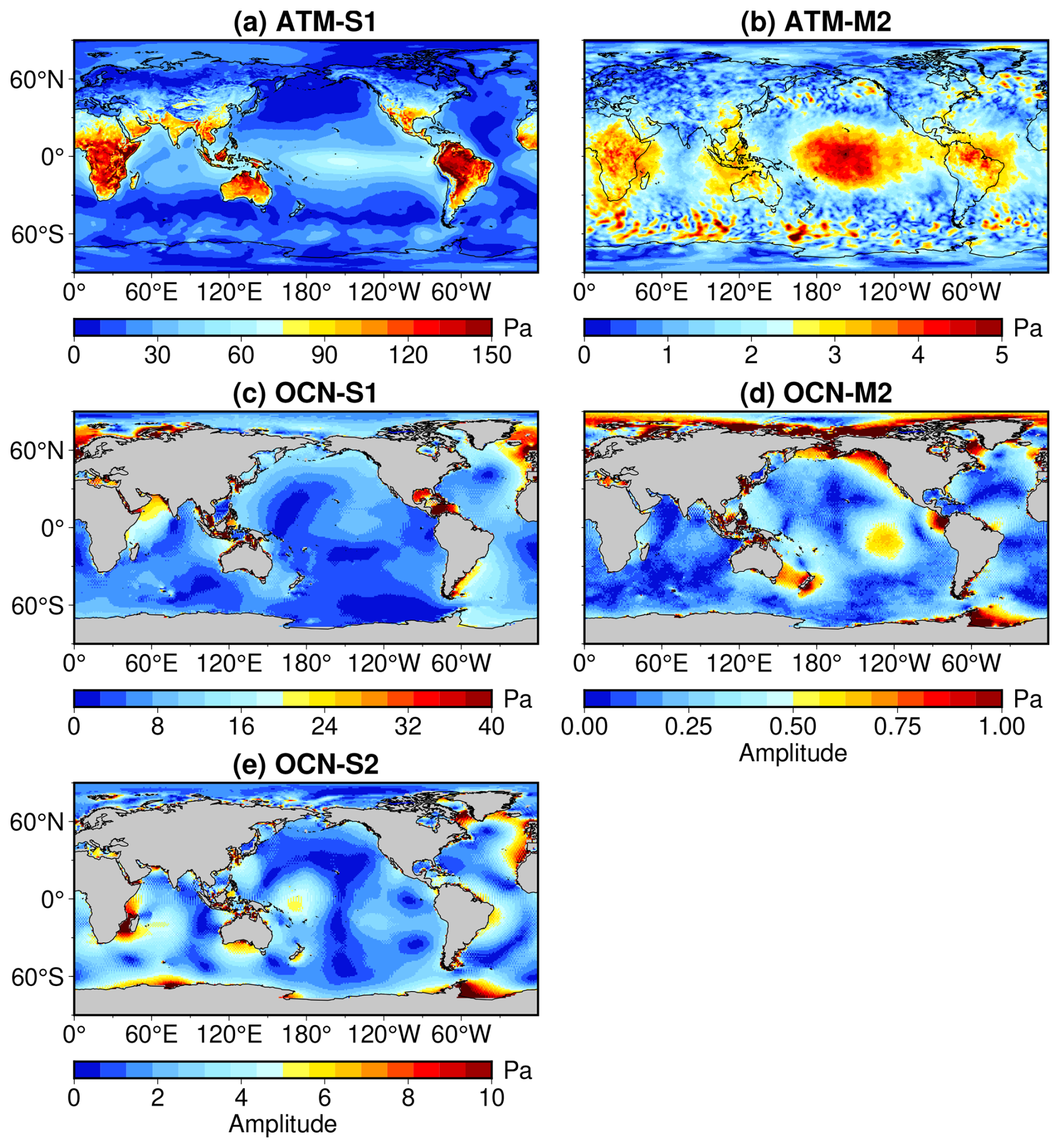
Figure 4 Amplitudes (Pa) of selected tidal constituents estimated from CRA-LICOM over 2007–2014. The top panels show atmospheric tides based on 6 hourly data: (a) S₁ and (b) M₂. The middle and bottom panels demonstrate oceanic tides derived from 3 hourly data: (c) S₁, (d) M₂, and (e) S₂.

In correspondence, the oceanic tidal constituents S₁ and M₂ derived from the oceanic contribution to OBP are shown in Fig. 4c–d, respectively. Taking advantage of the high temporal resolution of the ocean model output, the semi-diurnal tide S₂ was also extracted and is shown in Fig. 4e. As illustrated, the three oceanic tidal constituents share similar spatial patterns with those reported in the AOD1B RL06 documentation (Dobslaw et al., 2016), but with notably smaller amplitudes, particularly for OCN-S2, whose maximum amplitude reaches ∼ 10 Pa in CRA-LICOM compared to ∼ 400 Pa in AOD1B RL06. These discrepancies are likely due to the absence of atmospheric surface pressure forcing in LICOM, and the relatively lower (6-hourly) temporal resolution of the forcing fields, which is insufficient to simulate semi-diurnal S₂ tide. These findings highlight potential directions for future improvements to the CRA-LICOM system, which are discussed further in Sect. 6. For verification, all the atmospheric and oceanic tidal constituents of CRA-LICOM are additionally presented in Fig. B3 of the Appendix B.

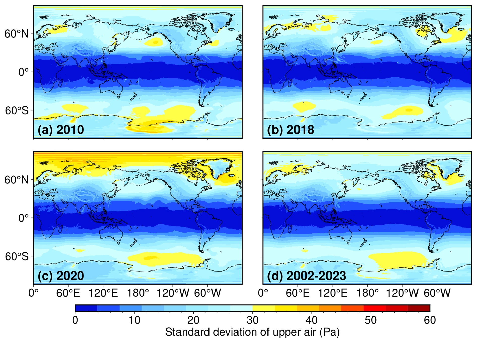
Figure 5 The standard deviation (Pa) of fields synthesized from upper air anomaly (mean field is removed) for (a) 2010, (b) 2018, (c) 2020, and (d) 2002–2023.

Another auxiliary product is the upper air anomaly, which is obtained by $I_n^v-I_n^s$ in Eq. (7) and thereby can be an indicator of multi-level atmospheric data quality. Although the magnitude is small compared to the surface pressure, the upper air anomaly constitutes a non-negligible component of the atmospheric dealiasing product (Swenson and Wahr, 2002). In Fig. 5, we calculate the standard deviation from various time periods to investigate the variation. The global mean of each scenario from Fig. 5a–d is found to be 17.43, 16.88, 17.75, and 17.34 Pa, respectively. Although this magnitude is much smaller than that of the total AO signal in Fig. 2, it has a magnitude as large as the amplitude of the major tides in Fig. 4, so it is not negligible. In addition, by comparing Fig. 5a–c to Fig. 5d, one can further see that upper air anomaly does not exhibit evident annual variation, and all preserve a similar spatial pattern. This fact suggests a rather stable contribution of upper air anomaly modeling due to the nature of regular atmospheric circulation.

5 Validation and Applications

5.1 Inter-comparison with GFZ-RL07

5.1.1 Temporal correlation and bias analysis in spectral/spatial domains

In this section, a straightforward comparison (against the official GFZ-RL07 product) is made at the product level itself. To assess the temporal performance of CRA-LICOM, temporal correlations and biases were evaluated in both the spectral and spatial domains.

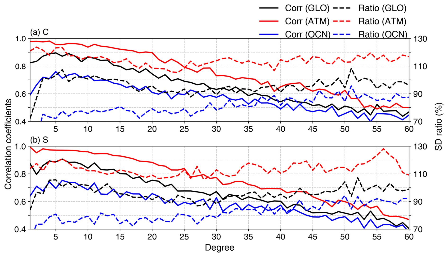
Figure 6 Mean temporal correlation coefficients (solid) and variation bias (dashed) for (a) C and (b) S of GLO (black), ATM (red) and OCN (blue) at each spherical harmonic degree between CRA-LICOM and GFZ-RL07 during 2002–2024.

First, in the spectral domain, the Stokes coefficients of CRA-LICOM and GFZ-RL07 products were analyzed for all degrees up to 60, for example. Figure 6 presents the mean temporal correlation coefficients of the Stokes coefficients per degree. At lower degrees (n<15), CRA-LICOM exhibits correlations exceeding 0.8, demonstrating fairly good agreement with GFZ-RL07 for gravity signals on a medium to large spatial scale. The consistency of low degrees is important since it is known that the AO model, as well as the GRACE gravity field, has its major energy at those degrees. As the degree increases, the correlation gradually decreases but remains statistically significant at the confidence level of 99 %. The peak correlation occurs at degree 5 for coefficient C (0.89) and degree 6 for coefficient S (0.90). Then, the standard deviation (SD) ratios of the two products were also analyzed to evaluate the variability biases; see the dashed curves in Fig. 6. CRA-LICOM generally slightly underestimates the variability coefficients compared to GFZ-RL07, with the SD ratios stabilizing over 90 % throughout the spectrum. Despite a decline at lower degrees, the ratio is constantly increasing from degrees 30 to 100, eventually reaching around 100 % at degree 100 (not shown), indicating CRA-LICOM's capability to reproduce high-frequency signals effectively.

Furthermore, the Stokes coefficients of ATM, representing atmospheric effects, and OCN, representing the dynamic oceanic contribution to OBP, are also shown in Fig. 6. Compared to OCN, the correlations between CRA-LICOM and GFZ-RL07 for ATM are consistently higher across all degrees, with smaller variation biases. As GLO reflects the combined effects of both ATM and OCN, its correlation and SD deviations lie between those of ATM and OCN. The correlation of ATM gradually decreases with increasing degree. For the first 20°, ATM maintains a high correlation, with coefficients exceeding 0.9; by around degree 50, the correlation drops to approximately 0.6. For OCN, the correlation of OCN peaks at degree 5 or 6, and since the peak the correlations gradually decline, reaching around 0.6 near degree 30. Furthermore, CRA-LICOM shows greater variability in ATM compared to GFZ-RL07. The SD ratio of ATM-C ranges from 105 % to 124 %, and that of ATM-S ranges from 106 % to 128 %. In contrast, CRA-LICOM exhibits weaker variability in OCN. For degrees below 30, the SD ratio remains around 80 %, gradually increasing thereafter but never exceeding 100 %. These findings suggest that atmospheric gravity variability in CRA-LICOM is closely aligned with those in GFZ-RL07, while discrepancies in oceanic gravity variations persist, likely reflecting uncertainties between models.

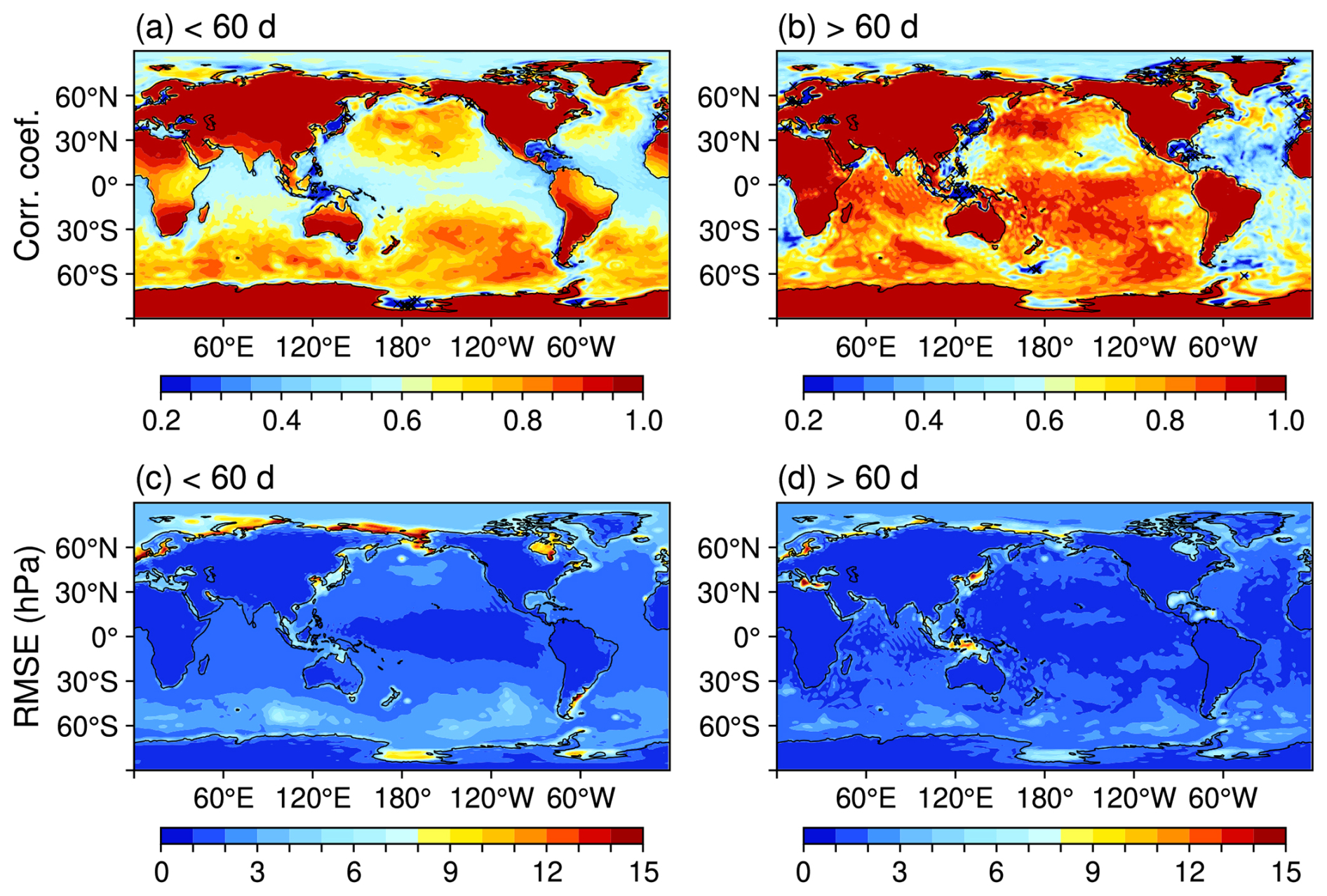
Figure 7 Temporal correlation coefficients (in terms of synthesized pressure fields) between CRA-LICOM and GFZ-RL07 during 2002–2023 for periods (a) <60 d and (b) >60 d. Panels (c) and (d) show the corresponding root mean square error (RMSE, hPa). In (a) and (b), locations marked with “×” indicate data not statistically significant at the 99 % confidence level. Frequency bands are separated using fourth-order Butterworth filters.

Then, evaluations are made in the spatial domain by projecting two products onto pressure fields on a regular grid 1° × 1°. To be consistent with the 1-month resolution of the present satellite gravity mission, the time-series pressure fields are decomposed into a frequency variability <60 d and another frequency variability >60 d. Figure 7a illustrates the temporal correlation coefficients for that <60 d, from which we see: (1) nearly all are statistically significant at a 99 % confidence level; (2) the correlations decrease with decreasing signal levels; (3) the correlations are substantially higher overland (0.85 on average) than over the ocean (0.63 on average). The high correlation over land indicates an overall consistency of atmospheric forcing fields employed, despite a few exceptions, such as Central Africa and the Northern region of South America, where the correlation coefficient degrades to around 0.7. We attribute this degradation as a consequence of the remaining S₂ atmospheric tide in CRA-LICOM since the spatial pattern resembles that of S₂ at a high similarity, see Yang et al. (2021). In contrast, S₂ has been removed from GFZ-RL07. For oceanic regions, mid- to high-latitudes have a correlation coefficient above 0.7, while it is lower at mid- to low-latitude oceans, particularly the Atlantic Ocean, and marginal seas exhibit weaker correlations down to 0.3, indicating a larger discrepancy between the two ocean models in these areas.

Furthermore, Fig. 7c illustrates the root mean square error (RMSE) of global temporal variability at a time window of <60 d. The global mean RMSE is found to be 1.79 hPa, while most pronounced biases are observed in the continental shelves and marginal seas of the Arctic Ocean, offshore China, and Hudson Bay, with RMSE peaks of up to 15 hPa. These discrepancies may result from differences in how the models represent topography, parameterization schemes (particularly wind stress), and the bottom friction law. The elevated RMSE in the Ross Sea can be attributed to LICOM's limited ability to simulate OBP in this region. Furthermore, notable biases are evident in the Southern Ocean, where the RMSE averages around 4 hPa, smaller than the SD value, approximately 8 hPa. These findings suggest that CRA-LICOM effectively captures consistent temporal variability amplitudes across most regions, except the marginal seas near continental shelves. Figure 7b and d demonstrate the correlations and biases for periods >60 d, revealing stronger correlations and smaller biases globally, while this has little impact on satellite gravity because its spectrum is slower than the aliasing frequency. The average correlation coefficients are 0.89 for the land and 0.71 for the ocean regions, with a global mean RMSE of as low as 1.29 hPa. This confirms the improved agreement between CRA-LICOM and GFZ-RL07 for longer periods. However, model uncertainties are more pronounced at higher frequencies, which poses a challenge for OBP simulations in the context of de-aliasing satellite gravity observations.

5.1.2 On-orbit validation via postfit KBRR-residuals

The observation of satellite gravity on orbit along the track, for example, the intersatellite K-band range rate (KBRR), is extremely sensitive to the geophysical process over regions where satellites fly (Ghobadi-Far et al., 2020). Therefore, KBRR, especially its residuals after removing essential background geophysical signals, including AO, can be an effective indicator of the quality of the AO model (Zenner et al., 2010; Yang et al., 2018). In particular, since the postfit KBRR residuals, obtained after least-square adjustment of the temporal gravity field, is more sensitive than the prefit KBRR to the mis-modeling error, we select the postfit KBRR residuals as the metric in this study. Here, we use data from Sect. 2.2.2 to calculate the postfit KBRR residuals for an initial diagnosis of two AO products, i.e., GFZ-RL07 and CRA-LICOM. All data processing to obtain the final KBRR residuals is manipulated by our open source Python software (namely PyHawk, https://github.com/NCSGgroup/PyHawk.git, last access: 1 February 2025, see also Wu et al., 2025), which indeed has achieved a complete data processing chain from Level-1b raw data to Level-2 temporal gravity fields.

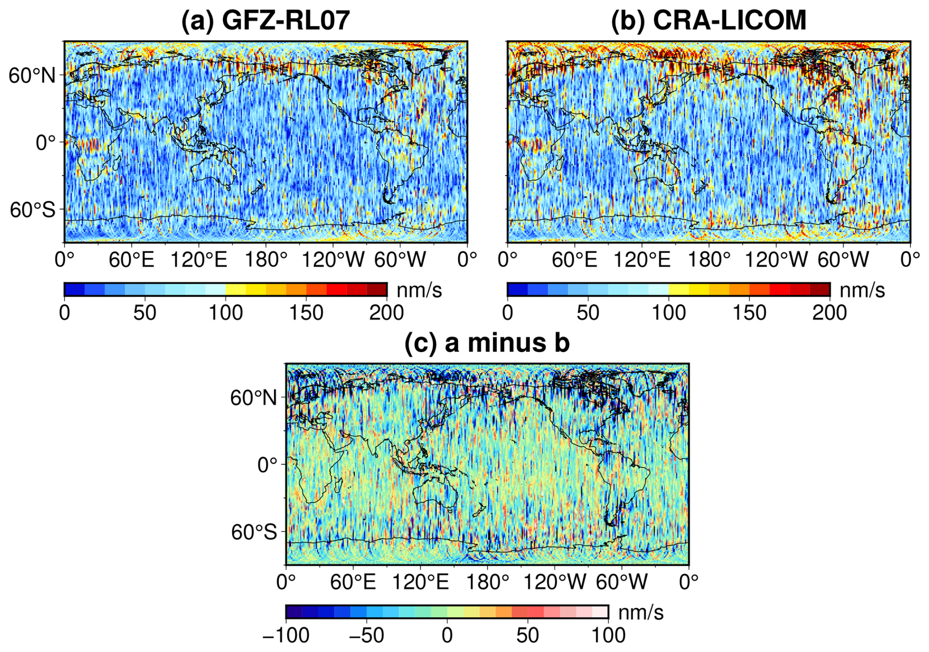
Figure 8 Postfit KBRR-residuals for GRACE using AO product, i.e., (a) GFZ-RL07 and (b) CRA-LICOM, respectively. One-month KBRR-residuals on December 2010 were firstly assembled as gridded RMS (root mean square) by GRACE's ground track (mid of twin satellites) and projected into a map of 1° × 1°. The grid with a negative value at the map (c, GFZ-RL07 minus CRA-LICOM) may indicate where GFZ-RL07 outperforms CRA-LICOM and vice versa.

Figure 8 illustrates the spatial map of the KBRR residuals in terms of gridded root mean square (RMS), where an arbitrary month is selected as an example. By comparing Fig. 8a to b, both scenarios, as expected, have demonstrated the successful removal of the major temporal gravity signals, so that the overall residuals are displayed as white noise. However, for example, in Fig. 8a, there are still some places where the residuals are obviously larger than the average, suggesting a greater uncertainty of the recovered signals in these places. In this sense, we may find in Fig. 8b that the uncertainty of CRA-LICOM is slightly stronger than that of GFZ-RL07. For a statistical study, we derive their differences in Fig. 8c. Since AO is utilized as a prior model to be removed from KBRR observations and the only difference between Fig. 8a and b is the AO model, one can always expect a smaller KBRR residual if the prior model better reproduces the reality. In Fig. 8c, the global mean of the differences is found to be −12.81 nm s⁻¹, which, as a negative value, suggests that CRA-LICOM is slightly more noisy. However, since the state-of-the-art KBRR is insensitive to noise less than ∼ 100 nm s⁻¹, the slight degradation of CRA-LICOM relative to GFZ-RL07 cannot be captured. Likewise, the global RMS of Fig. 8c is only 39.85 nm s⁻¹, which is also less than ∼ 100 nm s⁻¹. Furthermore, we exclude meaningless values by setting a threshold of 100 nm s⁻¹ in Fig. 8c; as a result, for the remaining data, the proportion (relative to the entire map) of positive and negative grids is 0.28 % and 2.38 %, respectively. The small proportion indicates that a majority of their differences are insensible, while GFZ-RL07 slightly outperforms CRA-LICOM due to a higher proportion of negatives. Also, be aware that GFZ-RL07 is better temporally resolved (3 h), which should also be responsible for its superiority.

5.1.3 Temporal gravity recovery and its error analysis

As one step further than in the previous section, we recover Earth's temporal gravity fields up to a degree/order of 60 for five years. The period from 2005–2010 was selected as an example to take advantage of GRACE's stable performance. Then, a series of standard post-processing steps of the gravity fields obtained were performed, which include (but are not limited to): (1) conversion of the gravity field to the equivalent height of water (EWH) on a gridded map of 0.5° × 0.5°, (2) replacement of low degree Stokes coefficients (Loomis et al., 2020), (3) spatial filtering, DDK3, to damp the noise (Kusche, 2007; Yang et al., 2024b), (4) removal of glacial isostatic adjustment (Caron et al., 2018), etc. Subsequently, a linear regression is performed to extract the climatology and residuals, to indicate the signal and noise level of the obtained gravity field. All the aforementioned post-processing and signal/error analyses are conducted using our open source Python software (called SaGEA, https://github.com/NCSGgroup/SaGEA, last access: 1 February 2025), which follows a standard workflow to handle the Level-2 gravity fields, see Liu et al. (2025b) for more details.

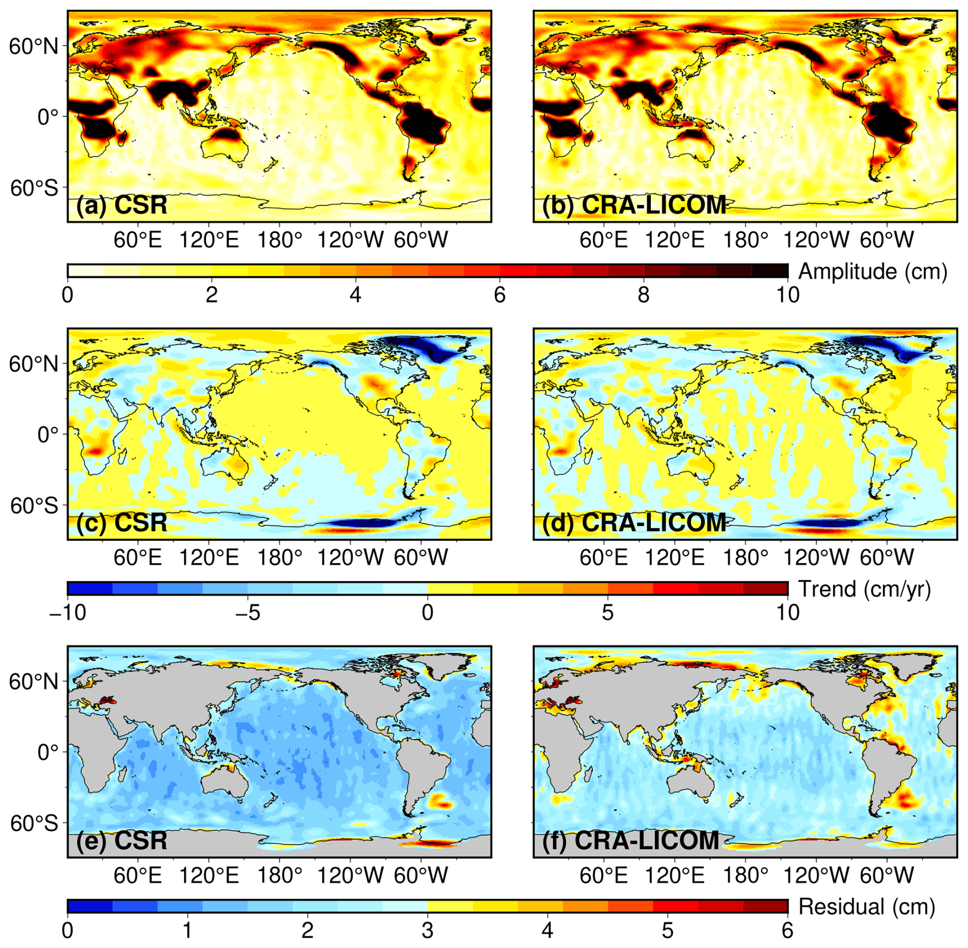
Figure 9 Temporal gravity field recovery (2005–2010, in terms of equivalent water height) using CRA-LICOM and its comparison against the latest CSR product. The signals, in terms of annual amplitude and secular trend, are demonstrated in (a)–(d); the error (or noise) level, indicated by standard deviation of ocean residuals with climatology removed, is present in the last row.

Figure 9 presents a detailed comparison between the latest official CSR gravity field product, which adopts the GFZ-RL07 AO model, and our derived gravity field solution (hereafter referred to as CRA-LICOM for consistency), which utilizes the CRA-LICOM AO model. The first two rows of the figure demonstrate that both solutions achieve comparable signal magnitudes. Specifically, the secular trend exhibits a high spatial correlation coefficient of 0.94, while the annual amplitude shows an even stronger correlation of 0.96, reinforcing that the CRA-LICOM constitutes a viable alternative AO model for current satellite gravity missions. However, a notable distinction arises in the noise characteristics of the two solutions. As evident in Fig. 9, our gravity field product exhibits a systematically higher noise level compared to the CSR solution, although this elevated noise remains within the documented uncertainty range of GRACE-derived gravity solutions (Chen et al., 2021). Furthermore, the spatial distribution of errors in Fig. 9e–f reveals a striking resemblance to the patterns observed in Fig. 7, particularly in regions such as the Ross Sea, Indonesian archipelago, Arctic coastal zones, Black Sea, and Baltic Sea. This spatial coherence strongly suggests that (1) the uncertainty of the AO model is a dominant contributor to the overall uncertainty in the derived gravity field and (2) the current AO model exhibits reduced reliability in these specific regions due to a likely incomplete representation of ocean dynamics or atmospheric coupling. A comprehensive discussion of these limitations, including potential avenues for model refinement, will be provided in Sect. 6. In addition to the AO model, we acknowledge that our processing skill for GRACE gravity field recovery, although robust, does not yet match the optimization of CSR in noise suppression. And this can also be responsible for the higher noise in our product.

5.2 Validation against OBP recorders and Argo observations

Direct observational data from OBP recorders were used to validate the OBP simulated by LICOM. Figure 10a–b present the SDs of six-hourly non-tidal OBP from both DART observations and CRA-LICOM simulations. Both datasets exhibit stronger OBP variability in the North Pacific compared to other regions of the open ocean. The mean SD across 68 site locations is 2.87 hPa, while the corresponding value from CRA-LICOM is slightly higher at 3.09 hPa. Figure 10c displays the relative biases between CRA-LICOM and DART, with an average bias of 18.7 % across the 68 locations. Notably, 41 out of the 68 stations (approximately 60 %) show relative biases within ± 50 %. However, substantially larger biases exceeding 100 % are observed for stations in the northeast of New Zealand and near the South American coast. These discrepancies may result from various factors, including model uncertainties, interpolation errors, and limitations inherent to in-situ observations.

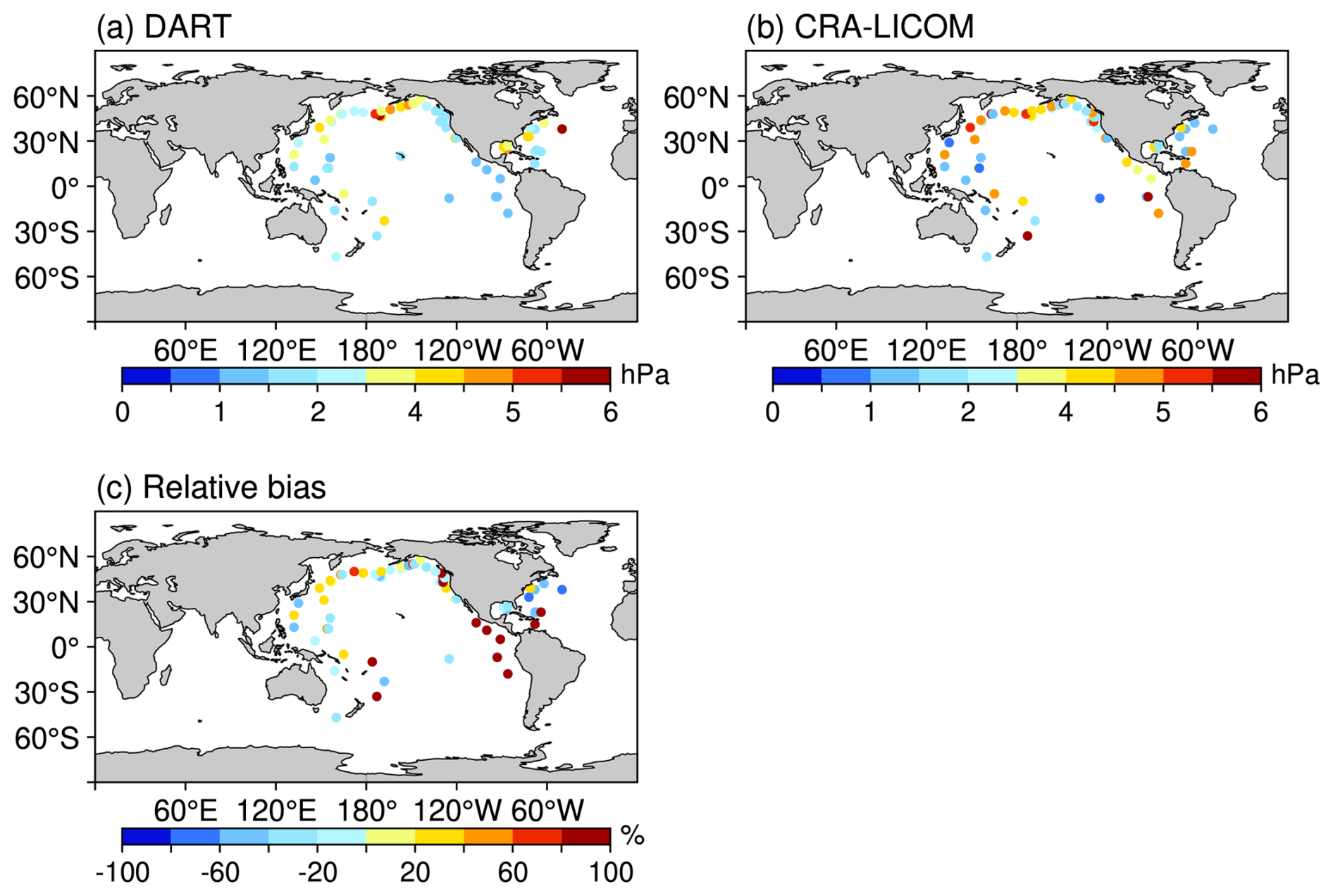
Figure 10 Standard deviations (hPa) of six-hourly non-tidal OBP from (a) DART and (b) CRA-LICOM during 2002–2023. Panel (c) shows the relative bias between CRA-LICOM and DART.

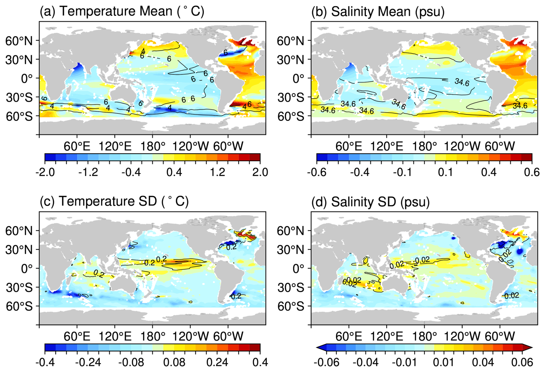
Figure 11 All the gridded value is derived as the average over vertical dimension by thickness-weight for the upper 2000 m. Time mean (a, b) and SD (c, d) are obtained from the period of 2005–2020. Across all subfigures, the selected variable from Argo is illustrated in contours as the reference, while the difference (i.e., CRA-LICOM minus Argo) is visualized in a shaded manner. The unit of temperature and salinity is °C and psu, respectively.

Another indirect validation is performed by investigating the key variables of ocean simulation, i.e., the temperature and salinity, which together define the density and eventually influence the bottom pressure. Figure 11 presents the difference in temperature and salinity in terms of temporal mean and SD between LICOM and Argo for the upper 2000 m during 2005–2020. We note that either temperature or salinity is computed as the vertical mean of the ocean up to 2000 m, which shall not be mentioned again for readability. As a reference, we report the global mean of the following variables from Argo: the temporal mean and SD of temperature is 6.22 and 0.14 °C; the temporal mean and SD of salinity are 34.69 and 0.014 psu; their spatial distribution can be somewhat inferred from the contours of Fig. 11 as well. Compared to this reference, the bias (CRA-LICOM minus Argo) in terms of global mean is much smaller: the temporal mean and SD of temperature is 0.025 and −0.030 °C; temporal mean and SD of salinity are 0.025 and −0.0027 psu. The bias in terms of relative percentage is 0.4 %, 21.4 %, 0.1 %, and 19.3 %, respectively, for these four variables. Although CRA-LICOM exhibits a slightly smaller variation (SD), be aware that the observations of Argo suffer from considerable uncertainty as well. Apart from this, all other evidence demonstrates an accurate simulation of the temperature and salinity of CRA-LICOM against in situ observations across the majority of the oceans, which further confirms the model's ability to capture upper-layer density and reproduce ocean states and variability. Furthermore, the variables simulated by LICOM are comparable to those of other leading ocean models (Tsujino et al., 2020; Treguier et al., 2023; Chassignet et al., 2020), providing a solid foundation for effective OBP simulations. However, the spatial heterogeneity revealed in Fig. 11 should also be taken into account. In particular, an increased bias could be seen in the tropical Pacific, the western coasts of the mid- to high-latitude Atlantic, and the Southern Ocean, indicating a greater uncertainty or potential problems of simulated temperature and salinity in these places. The next update of CRA-LICOM will focus on areas with significantly stronger bias or weaker SD.

5.3 Validation against Argo and Altimetry observations

On the one hand, satellite gravity (e.g. GRACE) can well reveal the total mass change of the ocean, i.e., water from land/glaciers into the ocean, if AO is perfectly removed; on the other hand, the accompanying monthly mean oceanic mass product (i.e., GAB; see Sect. 3.2.3) reflects the change in mass induced by the ocean current. In practice, as AO is imperfect, any AO product will leave a residual dynamic oceanic circulation signal to be picked up by GRACE. However, by convention, these two components together can be a measure of the manometric ocean (Gregory et al., 2019), and consequently, GRACE+GAB (or GAD with IB correction) has been widely used to investigate the change in global mean ocean mass (GMOM), see Uebbing et al. (2019). In addition, enforced by the ocean budget equation, Argo-induced steric ocean change and Altimetry-induced sea level rise, if the former is subtracted from the latter, allow for estimating GMOM change. Therefore, we used Altimetry-Argo as an independent external observation to validate the GRACE solution as well as our GAB product (from CRA-LICOM). Details on the description and access of the Altimetry and Argo data used can be found in Sect. 2.2.3.

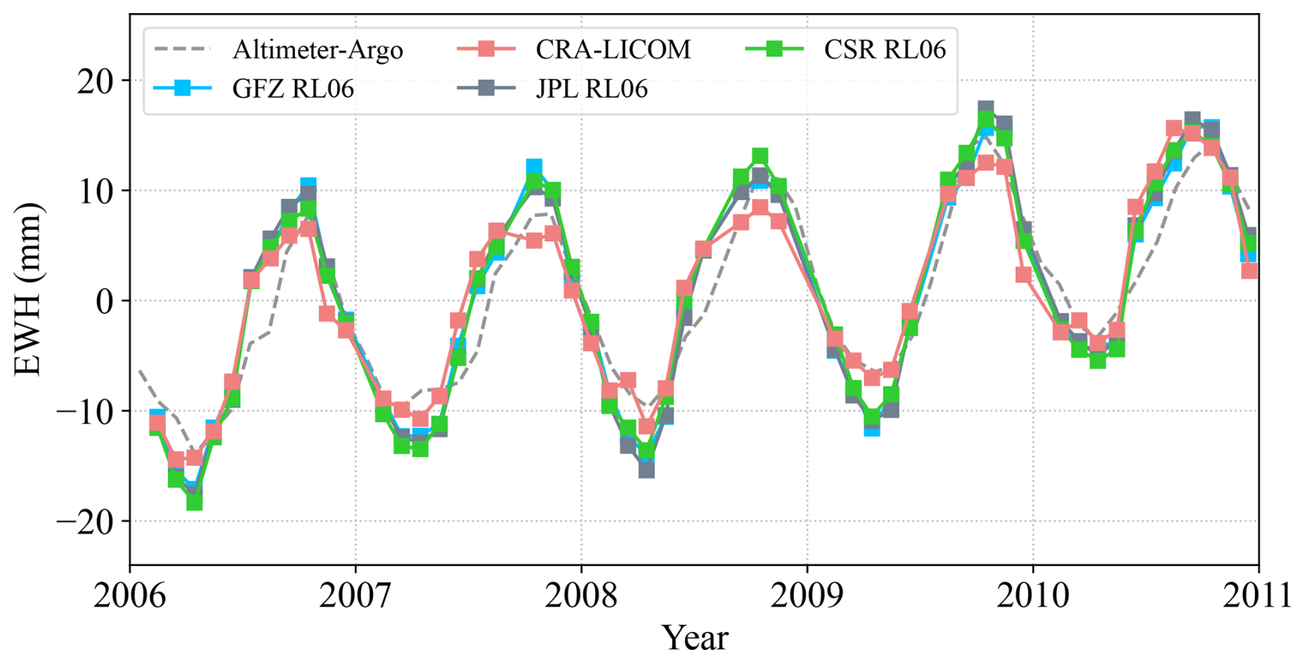
Figure 12 Global mean ocean mass change inferred from Altimeter‐Argo and various GRACE solutions. The GAB product from GFZ-RL07 is added back to GRACE's official gravity solutions, including CSR, GFZ, and JPL release 06. Instead, our GAB product from CRA-LICOM is added back to our GRACE gravity solution (see Sect. 5.1.3) for consistency.

Table 1 Secular trend and (semi-)annual amplitude of GMOM change inferred from Altimeter-Argo, or from GRACE+GAB.

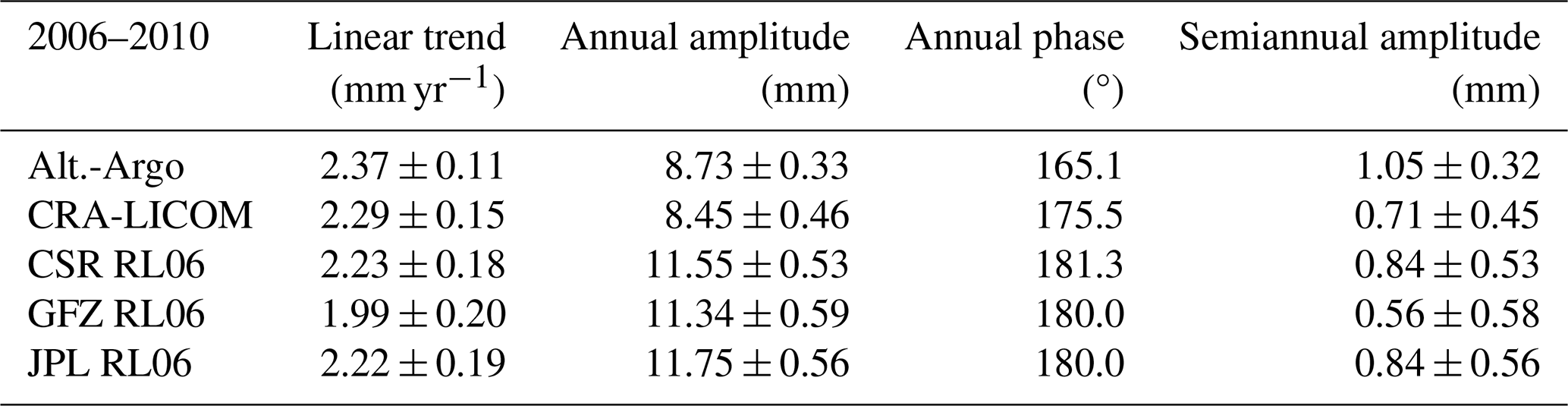
Here, we select three official GRACE Level-2 gravity field products (CSR RL06, JPL RL06, GFZ RL06, see Sect. 2.2.2 for more details) other than ours for a comparison. The gravity fields are first processed with the same procedures described in Sect. 5.1.3. The GAB is then added back and projected onto a 1° × 1° gridded EWH map. Finally, GMOM is derived for the global open ocean with a buffer area of 300 km to reduce leakages from continents to oceans (Chen et al., 2018). The variability is illustrated in Fig. 12, and the climatology indices are reported in Table 1. From Fig. 12, we see an overall agreement between Altimeter-Argo and GRACE+GAB in terms of variability, despite a slight annual phase delay of 10–15° (equivalent to approximately half a month). This systematic but small annual phase difference was previously reported by Chen et al. (2019), where ∼10° can be explained by the unintentional global mass non-conservation in GRACE gravity solution. Furthermore, from Table 1 one can see that CRA-LICOM has the least deviation from Altimetry-Argo, nearly closing the ocean budget in terms of secular trend and seasonality. However, the minor superiority of CRA-LICOM over others might warrant further verification. In addition, while various GRACE+GAB products exhibit a considerable discrepancy between each other, the discrepancy is still within the uncertainty (1σ as indicated in Table 1) and within the range reported by Uebbing et al. (2019). In other words, these products, including ours, are still statistically consistent, suggesting that CRA-LICOM has accepted accuracy for scientific applications without the need for special caution, particularly for large-scale studies.

6 Limitations

Despite the satisfactory accuracy of CRA-LICOM for scientific application, there is still a non-negligible discrepancy between CRA-LICOM and the official GFZ-RL07 product. Although a part of the discrepancy can be attributed to an inevitable uncertainty of both the forcing field and the ocean model, we also recognize that the current version of CRA-LICOM has some potential limitations that need to be addressed here and considered in the next round of updates. These limitations can be categorized into three main types: structural model uncertainty, parametric uncertainty, and input data uncertainty.

One major challenge arises from the structural uncertainty of the ocean model (LICOM). While our model's native horizontal resolution (equivalent to approximately 1°, see Appendix A) is comparable to the MPIOM model (1° on average, see Dobslaw et al., 2017) used by GFZ-RL07, the resolution of our model (due to different grid strategy) appears insufficient to accurately simulate the non-tidal dynamic OBP variations, especially at marginal seas near continental shelves. The 30 vertical levels employed in LICOM are also insufficient to resolve the first baroclinic mode (Stewart et al., 2017), which can affect the precision of the vertical integration of the seawater density. In addition, the lack of atmospheric pressure forcing in the model's momentum equations results in a weak response to atmospheric variability. The amplitudes of the oceanic tidal constituents are smaller than those reported in the AOD1B RL06 document due to lack of atmospheric pressure. Cheng et al. (2021) found that atmospheric pressure plays a key role in the variability of OBP in periods shorter than 10 d. Moreover, we claim that the current LICOM configuration used in this study lacks tidal mixing and self-attraction and loading (SAL) feedback to ocean dynamics (Ray, 1998; Shihora et al., 2022b). Although non-tidal dynamic OBP is the main focus, potential interactions between general ocean circulation and tidal flow regimes are non-negligible and should be taken into account (Thomas et al., 2001; Li et al., 2015); and Ghobadi-Far et al. (2022) also emphasized that SAL significantly affects coastal regions and enclosed seas, such as the Gulf of Carpentaria.

Another important source of discrepancy lies in the parametric uncertainty within the ocean model configuration. First, the representation of ocean bottom topography, which affects the magnitude and spatial patterns of the simulated OBP (Chen et al., 2023), is limited due to the relatively coarse horizontal/vertical resolution. Furthermore, the ocean mask that defines the distribution of ocean and land should also be responsible for the biases observed in marginal seas between two products. In particular, the Black Sea and the Caspian Sea are defined as land areas in our current configuration as a result of their small sizes. Other differences in ocean masks include the Antarctic ice shelves and the Arctic Ocean coastal area (particularly near the Beaufort Sea), where we may need a more accurate definition of LICOM. Last but not least, empirical parameters (e.g., for wind stress), the bottom friction law, and the selection of parameterization schemes for unresolved mixing and transport also influence the OBP simulations by LICOM.

An additional major challenge is that the atmospheric forcing field employed, at its current version, has a coarser vertical and temporal resolution than the ECMWF's latest reanalysis product used by GFZ-RL07. For example, multi-layer atmospheric reanalysis in terms of pressure level has been adopted for our atmospheric gravity modeling, which is likely not able to accurately reflect the upper air anomaly (Swenson and Wahr, 2002). Considering the fact that the impact of the upper air anomaly is not negligible, the forcing field is recommended at the model level rather than the pressure level (Yang et al., 2021; Shihora et al., 2022a). In addition, the sampling rate of our forcing field is only available for 6 h, restricting the number of feasible tides; for example, a major atmospheric tide S₂ (at a frequency of 12 h) is not allowed for the insufficient sampling rate. Likewise, many other smaller atmospheric tides, as well as oceanic tides, are not estimated and removed from CRA-LICOM, while this has been done in GFZ-RL07. As a consequence, the deficiency in atmospheric and oceanic tides will eventually influence the non-tidal counterparts. Furthermore, the 6 h resolution of CRA-40 may also limit the representation of high-frequency variations in OBP simulations compared to the 3 h atmospheric forcing fields used in GFZ-RL07 products.

7 Data availability

CRA-LICOM products are freely available at https://doi.org/10.11888/SolidEar.tpdc.302016 (Liu et al., 2025a). The products include Stokes coefficients for 6 h (ATM, OCN, GLO, and OBA), the corresponding monthly variables (GAA, GAB, GAC, and GAD), and the atmospheric tides.

8 Conclusions

We have established a new high-frequency atmospheric and oceanic gravity de-aliasing product, called CRA-LICOM, with a resolution of 6 h and 50 km and a coverage of 2002–2024 at a global scale. Various inter-comparisons and validations confirm that CRA-LICOM can well represent Earth's high-frequency mass changes and has sufficient accuracy to achieve the goal of de-aliasing for present satellite gravity missions. Specifically, we draw the conclusions as follows.

1. CRA-LICOM has confirmed that AO is the dominant source of high-frequency gravity signals (much larger than H), especially within the spectrum of aliasing, i.e., periods <60 d (twice the monthly sampling rate of GRACE).

2. CRA-LICOM is generally consistent with the official GFZ-RL07 in terms of the dominating long-wave gravity signal, where a high temporal correlation (>0.8) is found in the spectrum up to degree 15. Further spatial analysis confirms that the discrepancies are mainly within the aliasing spectrum (<60 d), which poses a challenge for satellite gravity missions. However, the two products demonstrate improved long-term consistency, i.e., the global mean temporal correlation coefficient increases from 0.71 to 0.77, and the global mean RMSE decreases from 1.79 to 1.29 hPa when transitioning from periods <60 d to >60 d.

3. Inconsistency of atmospheric/oceanic tidal constituents between CRA-LICOM and GFZ-RL07 contributes to the inconsistency of their non-tidal counterparts. For better consistency, one must not add back the atmospheric tide S₂ for orbit determination or GRACE gravity recovery using CRA-LICOM in practice.

4. The validation of the ocean model confirms that LICOM effectively captures the ocean state and variability, including temperature (mean bias < 0.4 %) and salinity (mean bias < 0.1 %), across most regions. However, significant biases are observed in the North Atlantic, Southern Ocean, and marginal seas near continental shelves, likely contributing to the errors of the OBP SD simulated by LICOM. The mean relative bias in non-tidal OBP SDs between CRA-LICOM simulations and DART in-situ observations is 18.7 % across 68 locations, with significantly larger biases (exceeding 100 %) at stations in the northeast of New Zealand and near the South American coast.

5. Temporal gravity recovery from GRACE using CRA-LICOM demonstrates a fairly high agreement (correlation coefficient >0.9) with GRACE's latest official products from CSR, JPL, and GFZ. Independent validation with Argo and Altimetry further confirms the ability of CRA-LICOM in large-scale ocean applications (such as global mean ocean mass change and barystatic sea level rise) and its consistency with other official gravity products.

6. As an independent product, CRA-LICOM could be a promising alternative to the official GFZ-RL07 product to be used in geoscience studies (GNSS, GRACE and other geodetic techniques). In particular, a full-time-scale uncertainty could be produced through an inter-comparison of CRA-LICOM and GFZ-RL07, which could also be a valuable complementary to GFZ's uncertainty product (Shihora et al., 2024). A better understanding of the uncertainty of the AO is essential for improving the current GRACE (-FO) as well as the design of the next-generation satellite gravity mission.

Appendix A: Fundamentals of LICOM model

LICOM is a global general circulation model developed by LASG/IAP since the late 1980s (Zhang and Liang, 1989). LICOM3.0 is currently the ocean component of two climate system models participating in CMIP6 (Coupled Model Intercomparison Project Phase 6): the Flexible Global Ocean-Atmosphere-Land System Model version 3 with a finite-volume atmospheric model (FGOALS-f3; He et al., 2020) and the version with a grid-point atmospheric model (FGOALS-g3; Li et al., 2020). In this study, we employ LICOM3.0 coupled with the Community Ice Code version 4 (CICE4) through NCAR flux coupler 7 (Craig et al., 2011; Lin et al., 2016), previously used for two Ocean Model Intercomparison Project (OMIP) experiments (Lin et al., 2020), to simulate OBP.

LICOM3.0 employs an orthogonal curvilinear coordinate system and a tripolar grid with a resolution of about 100 km with two poles located on land in the Northern Hemisphere at (65° N, 65° E) and (65° N, 115° W), which addresses the singularity issue at the North Pole inherent in traditional longitude-latitude grids. The horizontal grid employs the Arakawa B grid system with a resolution of approximately 1^∘, while the vertical eta coordinate system comprises 30 levels. These levels have a thickness of 10 m in the upper 150 m, gradually increasing to 713 m near the ocean floor. The bathymetry of the model is derived from ETOPO2 bathymetry data (https://ngdc.noaa.gov/mgg/global/etopo2.html, last access: 10 September 2018). Be aware that LICOM blocks the Antarctic ice shelves.

For equation discretization, the central difference advection scheme is applied in the momentum equations, while time integration uses the leapfrog method combined with a Robert filter. The tracer equations adopt a two-step shape-preserving advection scheme (Yu, 1994; Xiao, 2006) and semi-implicit vertical viscosity/diffusivity (Yu et al., 2018). The model computes the vertical viscosity and diffusivity coefficients using the scheme proposed by Canuto et al. (2001, 2002), while horizontal viscosity is represented using a Laplacian formulation, with coefficients set at 5400 m s⁻². To account for mesoscale eddy effects, LICOM3.0 employs the isopycnal tracer diffusion scheme of Redi (1982) and the eddy-induced tracer transport scheme of Gent and McWilliams (1990). In addition, the chlorophyll-a-dependent solar penetration scheme developed by Ohlmann (2003) is implemented.

Furthermore, Fig. A1 presents the annual mean time series of global mean temperature and salinity simulated by LICOM during six spin-up cycles under atmospheric forcing from 2002 to 2023. The SST and SSS reach equilibrium within six spin-up cycles. The relatively small trends in VOT and VOS result from the small imbalance in surface heat and freshwater fluxes, and no artificial drift remains in the system.

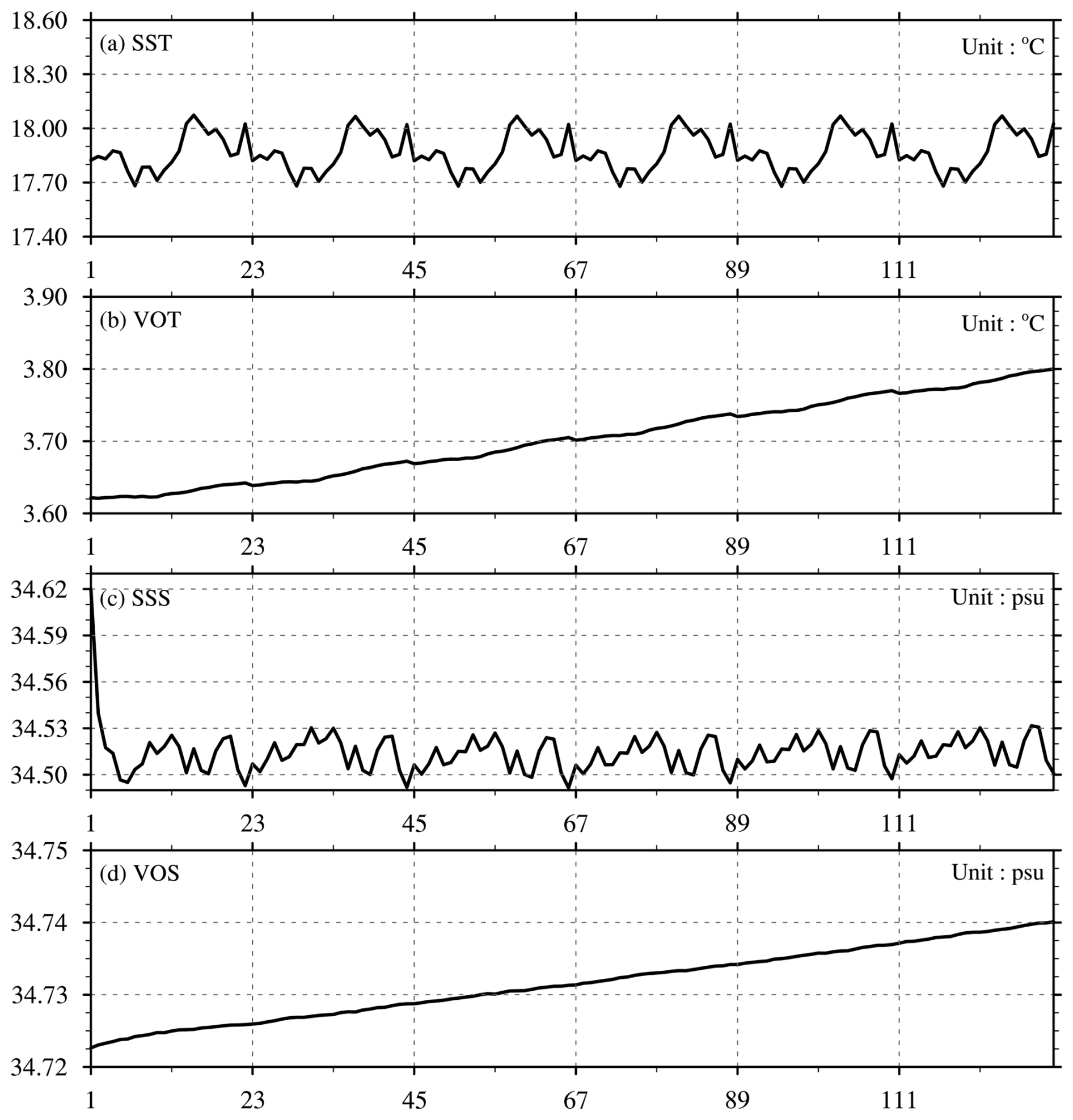
Figure A1 Annual global mean (a) sea surface temperature (SST; units: °C), (b) volume ocean temperature (VOT; units: °C), (c) sea surface salinity (SSS; units: psu), and (d) volume ocean salinity (VOS; units: psu) for CRA-LICOM during all the six cycles. The x-axis represents model time (units: Year).

Appendix B: Auxiliary experiments

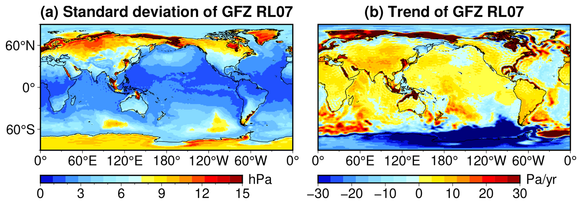
Figure B1 Equivalent pressure fields synthesized from GFZ-RL07 during 2002–present: (a) the standard deviation (hPa), (b) the secular trend (Pa yr⁻¹).

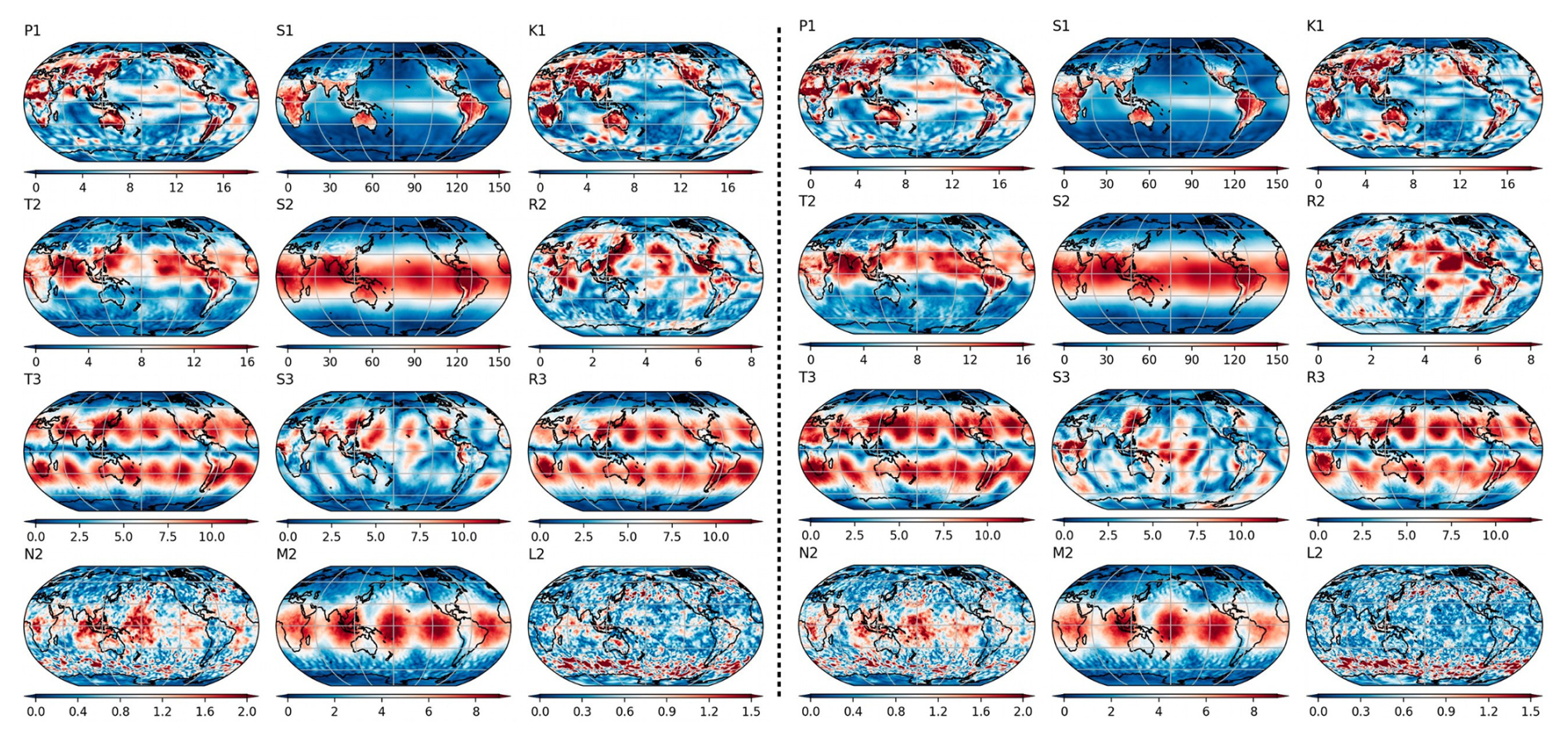
Figure B2 The left panel presents 12 atmospheric tides obtained from GFZ's official product, while the right panel presents our tides obtained from ECMWF-reanalysis (ERA-5) over the period 2007–2014. All tide lines are illustrated in terms of pressure amplitude [Pa]. See Dobslaw et al. (2016) for the definition of all tides.

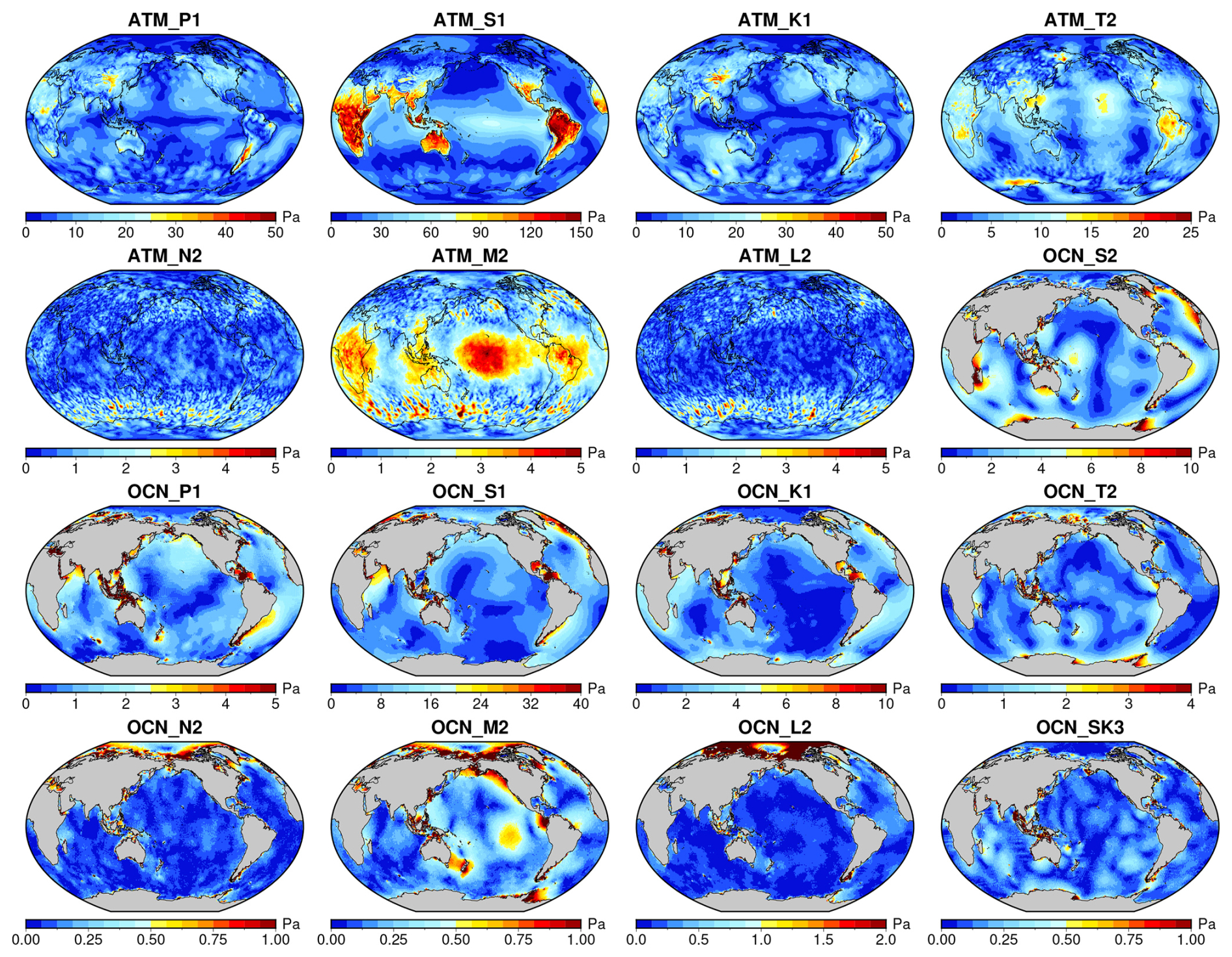
Figure B3 Amplitudes (Pa) of selected tidal constituents estimated by CRA-LICOM over 2007–2014. The first seven subfigures show atmospheric (ATM) tidal constituents, while the following nine subfigures present oceanic (OCN) tidal constituents.