TROPOMI Level 3 tropospheric NO₂ dataset with advanced uncertainty analysis from the ESA CCI+ ECV precursor project

We introduce the new ESA Climate Change Initiative TROPOspheric Monitoring Instrument (TROPOMI) global monthly clear-sky Level 3 (L3) dataset of tropospheric nitrogen dioxide (NO₂) for May 2018 to December 2021. The dataset provides spatiotemporally averaged tropospheric NO₂ columns, associated averaging kernels, and L3 uncertainties at spatial resolutions of 0.2, 0.5, and 1.0° on a monthly timescale (https://doi.org/10.21944/CCI-NO2-TROPOMI-L3, KNMI, 2025). To improve our understanding of what fraction of the Level 2 (L2) uncertainty cancels when averaging over space or time (i.e. the random component of the L2 uncertainty) and what fraction persists despite the averaging (systematic component), we first determine spatial and temporal error correlations for all sources of uncertainty in the L2 retrieval. Spatial error correlations arise mainly from the stratosphere–troposphere correction and from coarse-gridded albedo climatologies used in the L2 air mass factor calculation and have been quantified in previous studies. We find the temporal error correlation in both the stratospheric uncertainty and the air mass factor uncertainty to be 30 %. Using these estimates, the L3 uncertainty budget has been established for every grid cell based on input L2 uncertainties and new methods to estimate spatial and temporal representativeness uncertainties and to propagate measurement uncertainties through space and time. The total relative uncertainty in the resulting L3 dataset is in the range of 15 %–20 % in polluted areas, which is significantly lower than in individual L2 orbit retrievals, and brings the tropospheric NO₂ data to within the Global Climate Observing System (GCOS) “goal” and “breakthrough” requirements. Validation of the tropospheric, stratospheric, and total columns confirms better correlation and reduced dispersion in the differences between satellite and ground-based reference data for the L3 data with respect to the underlying L2, albeit with a more pronounced negative bias in the tropospheric columns at pollution hot spots, most probably related to stronger spatial smearing.

1 Introduction

Long-term monitoring of nitrogen oxides (NO_x = NO + NO₂) in the atmosphere is crucial for several reasons. Nitrogen oxides are harmful air pollutants, and long-term exposure is causally linked to chronic respiratory diseases and mortality in humans (Faustini et al., 2014; Fischer et al., 2015). When nitrogen dioxide (NO₂) is oxidised in the atmosphere, it forms nitric acid (HNO₃), which readily dissolves in airborne droplets and subsequently comes down as acid rain. Excessive deposition of HNO₃ has been shown to lead to adverse feedbacks on land and water ecosystems (Tan et al., 2020), and changes in N-deposition influence ecosystem carbon sinks, affecting the biosphere’s capacity to capture carbon from the atmosphere in the long run (Liu et al., 2022). Moreover, the monitoring of NO_x concentrations helps to identify major sources of CO₂, because both species are co-emitted upon combustion of fossil fuels by vehicles, industrial activities, and power plants (e.g. Zhang et al., 2023). Finally, NO_x play a significant role in the formation of ozone smog (Zhang et al., 2021) and fine particulate matter (Zhang et al., 2015), and both these secondary pollutants further harm human health and the environment. The importance of nitrogen oxides and their indirect impact on methane, ozone, and aerosol is an important reason why tropospheric NO₂ columns along with other trace gases have been selected as the so-called essential climate variable (ECV) precursors for aerosols and ozone (Zemp et al., 2022).

To allow for policy development and air pollution and climate change assessments, inter-annual changes and trends in recent decades need to be calculated. For this, long-term, robust, sustainable, and scientifically sound climate data records (CDRs) are needed to provide trustworthy information on how, where, and to what extent nitrogen oxide concentrations are changing. The European Space Agency (ESA) Climate Change Initiative (CCI) set out to develop robust satellite data records of key components of the climate system, including nitrogen dioxide concentrations. Atmospheric monitoring of NO_x involves application of in situ measurement techniques from ground-based or airborne platforms, but these measurements are limited in their spatio-temporal coverage. Satellite remote sensing with UV/Vis sensors, by contrast, has provided global measurements of tropospheric NO₂ columns since the mid-1990s. The wide spatial coverage and continuity of satellite measurements make them fit for purpose for climate monitoring. Among the key satellite instruments used to monitor tropospheric NO₂ columns are OMI (Ozone Monitoring Instrument) on NASA's Aura satellite and TROPOMI (TROPOspheric Monitoring Instrument) on ESA's Sentinel-5 Precursor, which provide long-term, high-resolution datasets critical for understanding air pollution trends.

Level 2 (L2) retrieval algorithms to derive NO₂ columns from raw satellite measurements (Level 1 data) have received a lot of attention (e.g. Van Geffen et al., 2022a). A framework for the evaluation of quality assurance measures was created in the Quality Assurance for Essential Climate Variables (QA4ECV) project for multiple climate variables including NO₂ columns for the L2 products of a group of sensors (not including TROPOMI) (Nightingale et al., 2018), providing users with evidence-based confidence in the products and enabling judgement on the fitness for purpose for specific applications. In comparison, Level 3 (L3) data, spatially and/or temporally averaged products on a consistent grid derived from L2 data (e.g. Wei et al., 2022), have been less considered by the scientific community. However, L3 data are relevant for model evaluation (Visser et al., 2019; Eskes et al., 2024), data assimilation (Inness et al., 2019; Sekiya et al., 2022), and climate (trend) studies (e.g. Zara et al., 2021). The emphasis on L2 retrieval algorithms is understandable, as it reflects the need to ensure the foundational accuracy of the L2 data, which is the starting point for creating high-quality L3 products. However, the quality of L3 products not only depends on reliable input data, but also requires a good understanding of best methods for averaging both spatially and temporally and assessing the propagation of existing measurement uncertainties and the quantification of additional sampling uncertainties.

Including rigorous uncertainty information in L3 CDRs is important to support the application of the data (Merchant et al., 2017). This is necessary to avoid misinterpretation of artefacts arising from system limitations such as real geophysical changes or trends (e.g. Labzovskii et al., 2024), for modellers to get confidence in discriminating model–data discrepancies that unambiguously indicate model deficiencies from those where observational errors are significant, and to contribute appropriate weighting to different observations in data assimilation and reanalyses (Merchant et al., 2017). An accurate quantification of L3 uncertainties includes both the assessment of the magnitude of error sources, as well as a propagation of these uncertainties to the L3 data product, including a treatment of spatio-temporal error correlations between individual satellite observations and of aspects of spatio-temporal representativity.

Measurement uncertainties are often assumed to be either fully systematic or fully random in space and time when determining gridded datasets (e.g. Wenig et al., 2008; Chan et al., 2023). In reality, there will be spatial and temporal correlations between multiple error sources, depending on length scale and timescales. There are datasets where uncertainties are determined using partial error correlations, but until now the correlation coefficients used have been determined using expert opinion, introducing subjectivity (Miyazaki et al., 2012; Boersma et al., 2016, 2018). A more quantitative treatment of spatial error correlations and representativeness errors in case of incomplete coverage of a grid cell has been presented in Rijsdijk et al. (2025). Their analysis reveals a grid-size-dependent partially systematic error contribution from the air mass factor and a fully systematic error from the stratospheric column. A detailed analysis of the effect of systematic sampling due to cloud cover resulted in a mathematically derived realistic spatial representation error. Rijsdijk et al.'s methods to reconstruct realistic uncertainties in spatial averages will be discussed in more detail in Sect. 3.2.2. In this paper we extend this spatial-averaging approach presented in Rijsdijk et al. (2025) to spatio-temporally averaged L3 products (gridded monthly means). This brings us to the following research questions for this study: (1) Can we improve our understanding of how uncertainties in satellite-derived tropospheric NO₂ columns are correlated in space and in time? (2) Can we use this understanding of correlations in uncertainties to better characterise how these uncertainties propagate into gridded, monthly mean uncertainty estimates? (3) What is the monthly mean uncertainty budget for TROPOMI NO₂ L3 data, and how do these L3 uncertainties vary in space and time? (4) To what extent does the validation with independent reference measurements help to assess the quality and fitness for purpose of the TROPOMI NO₂ L3 data?

We present the ESA CCI+ L3 TROPOMI atmospheric NO₂ dataset with a thorough assessment of the L3 uncertainty, combining measurement uncertainties, sampling uncertainties, and a proper assessment of local error correlations for the uncertainty propagation. This includes, for the first time, an empirical quantification of correlation coefficients for multiple error sources.

2 Instrument and dataset

2.1 TROPOMI instrument

The TROPOspheric Monitoring Instrument (TROPOMI) (Veefkind et al., 2012) provides data on tropospheric NO₂ (and many other trace gases) columns with daily global coverage at spatial resolution of 7×3.5 km² and, since 6 August 2019, of 5.5×3.5 km² at nadir. TROPOMI is aboard the European Space Agency (ESA) Sentinel-5 Precursor (S5P) satellite, which was launched on 13 October 2017 and has been providing nominal observations since May 2018. The near-polar sun-synchronous orbit provides afternoon observations with an Equator local overpass time of 13:30 and a nearly daily global coverage.

2.2 TROPOMI Level 2 tropospheric NO₂ columns and uncertainties

The starting point for the generation of L3 data is the L2 TROPOMI NO₂ tropospheric vertical columns on an orbital basis (Copernicus Sentinel-5P, 2021a). The aim of the ESA CCI+ project is to generate long-term climate data records, and therefore we use the TROPOMI PAL v2.3.1 L2 data, which are the most consistent with the OMI QA4ECV v1.1 product (Boersma et al., 2018). These OMI and TROPOMI data products are based on strongly consistent algorithms that use the same OMI surface albedo climatology (the so-called MINLER; Kleipool et al., 2008), which allows for better merging of the datasets and allows using data from 2004 to 2022. Still, the methods described in this paper are applicable on the operational dataset or any other version of the L2 data as well. TROPOMI retrievals with qa_value of > 0.75 were used, which corresponds to good-quality retrievals over (nearly) cloud-free scenes. Retrievals made in the descending part of the orbit are removed because high-latitude retrievals in the descending part of the orbit are not being used in the stratospheric correction procedure, leading to high-biased stratospheric NO₂ columns and, on average, negative tropospheric NO₂ columns for the descending part of the orbit (see Appendix A). A small bug with respect to the qa_value over snow and ice present in version 2.3.1 was corrected in this study (following the procedure set out in Sect. 5.1 in van Geffen et al., 2024).

The NO₂ retrieval procedure consists of three steps: the spectral fitting, the stratospheric correction, and the conversion of the tropospheric slant column density (SCD) into a tropospheric vertical column density using the air mass factor. Each of these three steps introduces potential errors and contributes to the overall uncertainty. The single tropospheric column uncertainty (σ_i) is quantified as in Boersma et al. (2004): ${\mathit{\sigma }}_i=\sqrt{{\left({\mathit{\sigma }}_{N_{\mathrm{s}}}\right)}^{\mathrm{2}}+{\left({\mathit{\sigma }}_{N_{\mathrm{s}}^{\mathrm{strat}}}\right)}^{\mathrm{2}}+{\left({\mathit{\sigma }}_{M^{\mathrm{tr}}}\right)}^{\mathrm{2}}}$, where the tropospheric column uncertainty sources are

$${\mathit{\sigma }}_{N_{\mathrm{s}}}={\displaystyle \frac{{\mathit{\sigma }}_{N_{\mathrm{s}}}^{\prime }}{M^{\mathrm{tr}}}};{\mathit{\sigma }}_{N_{\mathrm{s}}^{\mathrm{strat}}}={\displaystyle \frac{{\mathit{\sigma }}_{N_{\mathrm{s}}^{\mathrm{strat}}}^{\prime }}{M^{\mathrm{tr}}}};{\mathit{\sigma }}_{M^{\mathrm{tr}}}={\displaystyle \frac{(N_{\mathrm{s}}-N_{\mathrm{s}}^{\mathrm{strat}})\cdot {\mathit{\sigma }}_{M^{\mathrm{tr}}}^{\prime }}{(M^{\mathrm{tr}}{)}^{\mathrm{2}}}},$$

with N_s the slant column density; $N_{\mathrm{s}}^{\mathrm{strat}}$ the stratospheric slant column density; M^tr the tropospheric air mass factor; and ${\mathit{\sigma }}_{N_{\mathrm{s}}}^{\prime }$, ${\mathit{\sigma }}_{N_{\mathrm{s}}^{\mathrm{strat}}}^{\prime }$, and ${\mathit{\sigma }}_{M^{\mathrm{tr}}}^{\prime }$ their respective uncertainties.

The slant column density uncertainty ${\mathit{\sigma }}_{N_{\mathrm{s}}}^{\prime }$ is estimated on a per-pixel basis during the spectral fitting and is obtained from the diagonal of the covariance matrix of the standard errors (Van Geffen et al., 2020) and has typical values of ∼ 0.6 × 10¹⁵ molecules cm⁻² (Van Geffen et al., 2020, 2022a). This value compares well with values obtained with an alternative method to estimate uncertainties in the NO₂ slant column densities (by statistical analysis of the distribution of SCDs corrected for viewing geometry over regions with very little variability in stratospheric NO₂, reported in Boersma et al., 2004, Zara et al., 2018, and, most recently, for TROPOMI, in Van Geffen et al., 2020).

TM5-MP is being used in the TROPOMI NO₂ retrieval algorithm by providing estimates of stratospheric NO₂ columns. TM5-MP is a global chemistry-transport model that simulates atmospheric trace gas distributions at 1° × 1° resolution in the troposphere and in the stratosphere (Williams et al., 2017). The stratospheric slant column uncertainty ${\mathit{\sigma }}_{N_{\mathrm{s}}^{\mathrm{strat}}}^{\prime }$ is based on a global statistical analysis of results from the data assimilation procedure used to separate the tropospheric and stratospheric columns. The data assimilation procedure uses the observed slant columns and TM5-MP 24 h forecast stratospheric NO₂ fields (after modelled transport and chemistry). The difference between modelled forecasts and the actual observations (O–F) over unpolluted scenes is taken as an upper limit of the uncertainty in stratospheric NO₂ columns and has a statistical global-mean value of 0.2×10¹⁵ molecules cm⁻² (Dirksen et al., 2011), which is applied in the L2 algorithm (van Geffen et al., 2022b). Here, we apply a more detailed latitude- and time-dependent L2 stratospheric uncertainty as derived by Rijsdijk et al. (2025), where the O–F is analysed over latitudinal and day-of-year bands, resulting in a look-up table. A recent comparison of stratospheric NO₂ columns obtained with data assimilation in TM5-MP and the STREAM approach (Beirle et al., 2016), an alternative method to separate the stratosphere and troposphere columns, for GOME-2A showed consistency to within 0.2×10¹⁵ molecules cm⁻² (Richter et al., 2024). Similar results were found in a comparison of stratospheric NO₂ columns from the data assimilation method and STREAM for OMI of the QA4ECV dataset (Boersma et al., 2018; Compernolle et al., 2020) and are to be expected when applied to TROPOMI.

The air mass factor (AMF) uncertainty ${\mathit{\sigma }}_{M^{\mathrm{tr}}}^{\prime }$ consists of uncertainty contributions from the cloud pressure, cloud fraction, surface albedo, and a priori NO₂ profile shape. The theoretical error propagation framework in Boersma et al. (2004) is used to estimate the overall AMF uncertainty. The overall tropospheric AMF uncertainties are estimated to be 30 %–50 % (Boersma et al., 2018) for individual retrievals.

The overall uncertainty for an individual retrieval therefore depends on details in the retrieval and is pixel specific. Over oceans and remote areas, with low tropospheric vertical columns, the relative overall uncertainty is typically more than 100 % and is dominated by uncertainty in the spectral fit (${\mathit{\sigma }}_{N_{\mathrm{s}}}$) and the stratospheric slant column density (${\mathit{\sigma }}_{N_{\mathrm{s}}^{\mathrm{strat}}}$) (van Geffen et al., 2022b). For more polluted regions over continental areas, the relative uncertainty reduces to 25 %–50 % and is dominated by uncertainty in the tropospheric air mass factor (${\mathit{\sigma }}_{M^{\mathrm{tr}}}$) (van Geffen et al., 2022b). The overall uncertainty for individual TROPOMI tropospheric vertical column NO₂ retrievals ($N_{\mathrm{v}}^{\mathrm{trop}}$) is sometimes approximated as ${\mathit{\sigma }}_i\approx \mathrm{0.5}\times {\mathrm{10}}^{\mathrm{15}}$ molecules cm${}^{-\mathrm{2}}+[\mathrm{0.2}$ to $\mathrm{0.5}]\times N_{\mathrm{v}}^{\mathrm{trop}}$ (van Geffen et al., 2022b).

3 Methodology

3.1 L3 algorithm overview

Our starting point is individual L2 tropospheric vertical column retrievals with a retrieved column value x_i (molecules cm⁻²) and the associated individual retrieval uncertainty σ_i (molecules cm⁻²). To compute L3 spatial and temporal gridded means, we developed a two-step procedure, in which we

1. calculate spatially averaged (gridded) column values (x_o,t) – where t stands for an instantaneous column value not averaged in time – along with their associated L2 measurement uncertainties (σ_m) and spatial representativeness uncertainty (σ_rs), combined into the spatial average uncertainty (σ_o,t). Here we follow the spatial averaging approach and uncertainty assessment described in Rijsdijk et al. (2025).

2. provide temporal averaged estimates ($\overline{x}$) of the spatially averaged column values (x_o,t) and their total uncertainty (${\overline{\mathit{\sigma }}}_{\mathrm{total}}$), including associated temporal representativeness uncertainty (${\overline{\mathit{\sigma }}}_{\mathrm{rt}}$) and measurement uncertainties (${\overline{\mathit{\sigma }}}_{\mathrm{m}}$).

Figure 1 provides a schematic picture of the above procedure. After collecting the individual values of the retrieved column (x_i) and its uncertainty (σ_i), their spatially averaged (instantaneous) counterparts (x_o,t, σ_o,t) are calculated for a L3 grid cell. Then, in Step 2, these spatial averages are aggregated over time and averaged, leading to the desired L3 product. This two-step method allows us to assess and apply different error correlation factors when propagating uncertainties spatially and temporally.

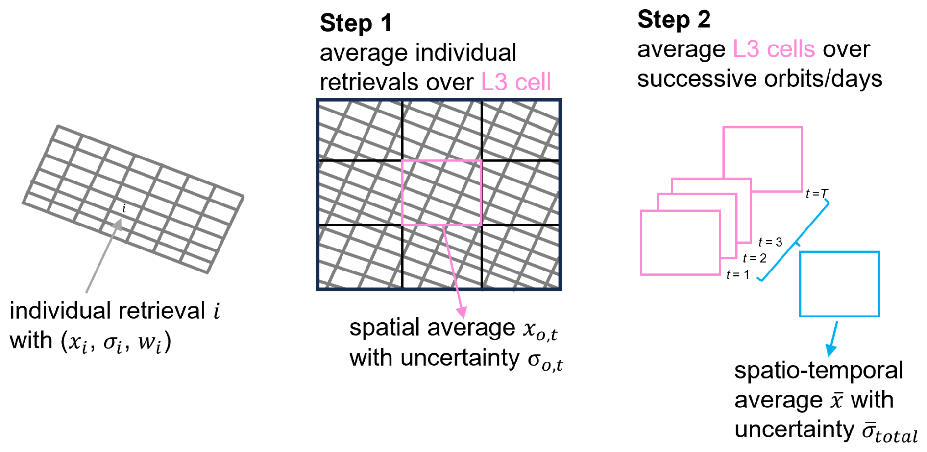
Figure 1 Schematic example of the procedure to calculate spatio-temporal (gridded) averages of retrieved columns and their associated uncertainties. The irregular grey rectangles indicate an ensemble of individual L2 retrievals in a satellite orbit; the black rectangle shows a regular grid to which the individual retrievals are averaged and gridded in Step 1. In Step 2, this procedure is repeated to obtain multiple spatial averages along with their associated uncertainties, which are then averaged over a period to produce a temporal mean and its associated L3 uncertainty.

3.2 Spatial averaging

3.2.1 Averaging of variables

Step 1 concerns the spatial averaging of valid retrieved values of the individual pixels (x_i) with weights (w_i). Following Miyazaki et al. (2012), Boersma et al. (2016), Rijsdijk et al. (2025) the weight w_i of each measurement is taken equal to the spatial overlap area between the footprint of observation i and the L3 grid cell. This tiling approach results in the following estimate of the gridded L3 column:

$$\begin{array}{}\text{(1)}& x_{\mathrm{o},\mathrm{t}}={\displaystyle \frac{{\sum }_{i=\mathrm{1}}^N\left(w_i{x}_i\right)}{{\sum }_{i=\mathrm{1}}^N{w}_i}},\end{array}$$

with N the number of valid L2 observations in the L3 cell.

The spatial average is determined on a (regular) grid on a per-orbit basis. This is possible for any given grid; we provide the dataset created here at spatial resolutions 0.2° × 0.2°, 0.5° × 0.5°, and 1° × 1°. The spatial average for a grid cell is only determined if the combined valid individual retrievals x_i cover at least 30 % of the grid cell, to avoid unrealistic uncertainty estimates in small data samples, following Rijsdijk et al. (2025).

3.2.2 Uncertainty estimate

To assess the overall uncertainty (σ_o,t) in x_o,t of these spatial averages, we follow the procedure in Rijsdijk et al. (2025) and combine the propagated measurement uncertainties (σ_m) and the spatial representativeness uncertainty (σ_rs) in quadrature:

$$\begin{array}{}\text{(2)}& {\mathit{\sigma }}_{\mathrm{o},\mathrm{t}}=\sqrt{({\mathit{\sigma }}_{\mathrm{m}}{)}^{\mathrm{2}}+({\mathit{\sigma }}_{\mathrm{rs}}{)}^{\mathrm{2}}}.\end{array}$$

This reflects that the uncertainty in the spatial average is composed of propagated L2 uncertainties and may also contain uncertainty from incomplete coverage of the grid cell.

Measurement uncertainty

The measurement uncertainty σ_m is the combined tropospheric vertical column uncertainty from error contributions (σ_m,c) in the L2 retrieval, including the uncertainty due to the slant column density measurements (${\mathit{\sigma }}_{N_{\mathrm{s}}}$), the uncertainty resulting from errors in the stratospheric column (${\mathit{\sigma }}_{N_{\mathrm{s}}^{\mathrm{strat}}}$), and the uncertainty from the air mass factor (${\mathit{\sigma }}_{M^{\mathrm{tr}}}$) (Boersma et al., 2004).

$$\begin{array}{}\text{(3)}& {\mathit{\sigma }}_{\mathrm{m}}=\sqrt{({\mathit{\sigma }}_{N_{\mathrm{s}}}{)}^{\mathrm{2}}+({\mathit{\sigma }}_{N_{\mathrm{s}}^{\mathrm{strat}}}{)}^{\mathrm{2}}+({\mathit{\sigma }}_{M^{\mathrm{tr}}}{)}^{\mathrm{2}}}\end{array}$$

Note that these are the contributions of each uncertainty source to the tropospheric vertical column uncertainty, not the source uncertainties themselves. Each of these (${\mathit{\sigma }}_{N_{\mathrm{s}}}$, ${\mathit{\sigma }}_{N_{\mathrm{s}}^{\mathrm{strat}}}$, and ${\mathit{\sigma }}_{M^{\mathrm{tr}}}$) is represented by Eq. (4) (Sekiya et al., 2022; Rijsdijk et al., 2025), which considers that the random component of the individual uncertainties σ_i tends to cancel out when averaging over many observations (first term on the right-hand side), while a fraction ϕ_c of the individual uncertainties σ_i persists after averaging because they come from systematic, spatially correlated contributions to the uncertainties (second term):

$$\begin{array}{}\text{(4)}& {\mathit{\sigma }}_{\mathrm{m},\mathrm{c}}=\sqrt{(\mathrm{1}-{\mathit{\varphi }}_{\mathrm{c}}){\displaystyle \frac{{\sum }_{i=\mathrm{1}}^N\left(w_i^{\mathrm{2}}{\mathit{\sigma }}_{i,\mathrm{c}}^{\mathrm{2}}\right)}{{\sum }_{i=\mathrm{1}}^N{w}_i^{\mathrm{2}}}}+{\mathit{\varphi }}_{\mathrm{c}}{\displaystyle \frac{\left({\sum }_{i=\mathrm{1}}^N\right(w_i{\mathit{\sigma }}_{i,\mathrm{c}}){)}^{\mathrm{2}}}{{\sum }_{i=\mathrm{1}}^N{w}_i^{\mathrm{2}}}}}.\end{array}$$

The spatial error correlation factor ϕ_c in Eq. (4) quantifies the portion of the error that is systematic, and here we determine its value for each of the measurement error contributions c (slant column density, stratospheric column, and air mass factor) separately. We apply the spatial error correlations as determined by Rijsdijk et al. (2025).

The slant column error is largely uncorrelated over space as it is dominated by measurement noise (Van Geffen et al., 2020; Rijsdijk et al., 2025). There will be a systematic error component in the slant column density due to gaps in knowledge, such as offsets in absorption cross sections, inaccurate ring coefficients in the spectral fit, or the lack of a correction for vibrational Raman scattering (Richter et al., 2011; Zara et al., 2018; Rijsdijk et al., 2025). In Van Geffen et al. (2020) the slant column retrieval noise estimated over a Pacific sector was found to match the DOAS uncertainty estimate to within 15 % for clear-sky pixels, suggesting systematic retrieval errors are roughly a factor of 2 smaller than the random errors. However, the effect of these systematic errors is absorbed in the stratospheric column estimate (as discussed below). Therefore, the uncertainty in slant column density is assumed to be fully random (${\mathit{\varphi }}_{N_{\mathrm{s}}}=\mathrm{0}$) (Rijsdijk et al., 2025).

In the retrieval method the stratospheric column is determined by assimilating slant column superobservations in the chemical transport model TM5-MP (Williams et al., 2017). The resolution of the TM5-MP model is 1° × 1°, and the horizontal correlation length scale used in the assimilation is about 500 km. This is coarser than the spatial average grid sizes of 0.2 to 1.0° considered here. Therefore, it is assumed that the error in the stratospheric column is fully correlated in space with the L3 grid resolution (${\mathit{\varphi }}_{N_{\mathrm{s}}^{\mathrm{strat}}}=\mathrm{1}$). A spatially correlated error in the slant column would lead to an increased bias in the O–F, increasing the L2 stratospheric column uncertainty. The spatial mean of the stratospheric column uncertainty in Eq. (3) will thus include the contribution from the systematic slant column uncertainty.

The AMF uncertainty is caused by a combination of components that go into the calculation of the AMF. The a priori NO₂ profile is a large contribution to the AMF uncertainty but is shown to become irrelevant when the averaging kernel is used when comparing with three-dimensional model output (Eskes et al., 2003). Other major components of the AMF uncertainty are the uncertainties in surface albedo and cloud parameters (cloud fraction and cloud pressure). All three of these variables depend on the quality of the climatological surface albedo dataset. Rijsdijk et al. (2025) review the AMF uncertainty by comparing versions 2.3.1 and 2.4 of the NO₂ L2 datasets. The main difference between these two versions is that they apply different surface albedo climatologies. We argue that the differences between albedo estimates from these state-of-science climatologies are indicative of realistic albedo uncertainties. The albedo values directly affect the clear-sky AMF calculations but also drive the retrieved values for the cloud fraction and cloud pressure (see e.g. Riess et al., 2021). Differences between albedo values thus propagate to different values of cloud fraction and cloud pressure, which impact the cloudy-sky AMF values. Albedo differences thus impact the overall AMF calculation, and spatio-temporal characteristics in the albedo differences are expected to lead to spatio-temporal patterns in AMF differences, allowing us to analyse how the AMF uncertainty patterns are correlated in time and space. The effects of changing the surface albedo climatology on the results of the tropospheric NO₂ retrieval are expressed as differences between v2.3.1 and v2.4 tropospheric NO₂ columns. The error in the AMF is shown by Rijsdijk et al. (2025) to be partly correlated depending on the size of the grid cells (${\mathit{\varphi }}_{M^{\mathrm{tr}}}=e^{-d/l}$, where d is a distance between observations depending on the grid cell size and l=35 km is a typical average correlation length over polluted regions). This spatial correlation is partly due to the low resolution of surface albedo datasets (0.5°) but also because surface modifying conditions are often spatially extensive. For example, droughts impact the surface albedo not just in one grid cell but typically over a larger area. Table 1 provides typical values of the spatial error correlation coefficients for TROPOMI spatial averages at different grid resolutions.

Table 1 Spatial error correlation sources and their random and systematic fractions for TROPOMI NO₂ tropospheric vertical column spatial averages at different spatial resolutions. For the calculation of the AMF coefficients, ${\mathit{\varphi }}_{M^{\mathrm{tr}}}=e^{-d/l}$ has been used with l=35 km the typical correlation length over polluted regions (Rijsdijk et al., 2025) and d the typical grid cell dimension (in km).

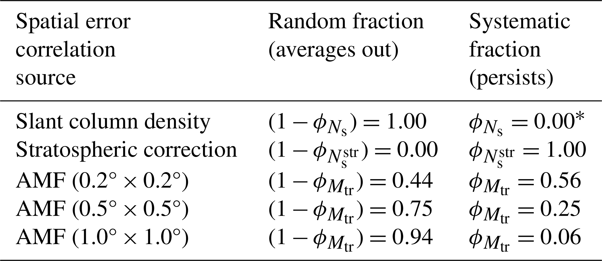
^∗ Note: the systematic component of the slant column density uncertainty is included in the stratospheric uncertainty.

Spatial representativeness uncertainty

The spatial representativeness uncertainty σ_rs (molecules cm⁻²) accounts for incomplete sampling (mainly due to cloud-covered pixels not being included in the spatial averaging) of the cell by the observations available to calculate x_o,t (Rijsdijk et al., 2025). If the entire area of the L3 cell is covered by valid observations, then the representativeness uncertainty is 0. If only a small fraction of the L3 cell is covered, the representativeness uncertainty is equal to the standard deviation of the tropospheric vertical columns within the cell: large for areas with strong spatial variability in x_i (such as over polluted regions) and smaller for regions with similar values of x_i (such as over clean, background regions).

$$\begin{array}{}\text{(5)}& {\mathit{\sigma }}_{\mathrm{rs}}=f{\mathit{\sigma }}_{x_i},\end{array}$$

where ${\mathit{\sigma }}_{x_i}$ is the standard deviation in retrievals within the grid cell. The unitless fraction f is calculated as the representativeness of the retrieved observations for the fully covered grid cell:

$$\begin{array}{}\text{(6)}& f={\displaystyle \frac{\mathrm{1}}{\sqrt{N_{\mathrm{eff}}{\mathit{\alpha }}_{\mathrm{o},\mathrm{t}}+\mathrm{1}}}}\sqrt{\mathrm{1}-{\mathit{\alpha }}_{\mathrm{o},\mathrm{t}}},\end{array}$$

where the degree of coverage α_o,t is calculated as the fraction of the total valid pixel area (A, in km²):

$$\begin{array}{}\text{(7)}& {\mathit{\alpha }}_{\mathrm{o},\mathrm{t}}={\displaystyle \frac{{\sum }_{i=\mathrm{1}}^N{w}_i}{A}},\end{array}$$

and N_eff is the number of effective observations, which is dependent on the number of available observations, the sensor, the trace gas, the L3 grid resolution, and whether a grid cell is sensitive to systematic sampling (e.g. due to a cloud field covering part of a grid cell) or not (Rijsdijk et al., 2025). The lower the value for N_eff, the more sensitive a region is to systematic sampling. N_eff has been determined empirically by Rijsdijk et al. (2025), and a summary of the methods used to quantify N_eff can be found in Appendix B.

3.3 Temporal averaging

3.3.1 Averaging of variables

The second step in the generation of the L3 dataset consists of temporal averaging, a method newly introduced in this study. We average the spatial-mean values (superobservations) x_o,t obtained in Step 1 over time (e.g. a period of 1 month), again in a weighted fashion to account for different degrees of representativity ($w_{\mathrm{o},\mathrm{t}}=\mathrm{1}-f$). f is high for grid cells with a large representativeness uncertainty and low for superobservations with almost no representativeness uncertainty. This value depends on coverage – higher coverage results in a lower representativeness error – as well as other factors such as sensitivity to systematic sampling. Taking a weighted average like this implies that superobservations with a low representativeness uncertainty obtain more weight in the temporal average than superobservations with a high representativeness uncertainty. This results in the following estimate of the spatially and temporally averaged L3 column $\overline{x}$:

$$\begin{array}{}\text{(8)}& \overline{x}={\displaystyle \frac{{\sum }_{t=\mathrm{1}}^T\left(w_{\mathrm{o},\mathrm{t}}{x}_{\mathrm{o},\mathrm{t}}\right)}{{\sum }_{t=\mathrm{1}}^T{w}_{\mathrm{o},\mathrm{t}}}},\end{array}$$

with T the total number of valid superobservations in the period over which the averaging is performed.

3.3.2 Uncertainty estimate

Next, the uncertainty associated with $\overline{x}$ (i.e. the monthly mean L3 uncertainty) is determined. We calculate a total spatio-temporal averaged uncertainty which combines the propagated measurement uncertainty (${\overline{\mathit{\sigma }}}_{\mathrm{m}}$, including the spatial representativeness uncertainty) and a temporal representativeness uncertainty (${\overline{\mathit{\sigma }}}_{\mathrm{rt}}$) in quadrature:

$$\begin{array}{}\text{(9)}& {\overline{\mathit{\sigma }}}_{\mathrm{total}}=\sqrt{({\overline{\mathit{\sigma }}}_{\mathrm{m}}{)}^{\mathrm{2}}+({\overline{\mathit{\sigma }}}_{\mathrm{rt}}{)}^{\mathrm{2}}}.\end{array}$$

Propagated measurement uncertainty

The spatio-temporally averaged measurement uncertainty ${\overline{\mathit{\sigma }}}_{\mathrm{m}}$ is the combined uncertainty of the measurement error contributions ${\overline{\mathit{\sigma }}}_{\mathrm{m},\mathrm{c}}$ including the spatial representativeness uncertainty and a priori profile uncertainty:

$$\begin{array}{}\text{(10)}& {\overline{\mathit{\sigma }}}_{\mathrm{m}}=\sqrt{({\overline{\mathit{\sigma }}}_{N_{\mathrm{s}}}{)}^{\mathrm{2}}+({\overline{\mathit{\sigma }}}_{N_{\mathrm{s}}^{\mathrm{strat}}}{)}^{\mathrm{2}}+({\overline{\mathit{\sigma }}}_{M^{\mathrm{tr}}}{)}^{\mathrm{2}}+({\overline{\mathit{\sigma }}}_{\mathrm{rs}}{)}^{\mathrm{2}}+({\overline{\mathit{\sigma }}}_{\text{a priori}}{)}^{\mathrm{2}}}.\end{array}$$

The propagated slant column density uncertainty (${\overline{\mathit{\sigma }}}_{N_{\mathrm{s}}}$), stratospheric column uncertainty (${\overline{\mathit{\sigma }}}_{N_{\mathrm{s}}^{\mathrm{strat}}}$), air mass factor uncertainty (${\overline{\mathit{\sigma }}}_{M^{\mathrm{tr}}}$), and spatial representativeness uncertainty (${\overline{\mathit{\sigma }}}_{\mathrm{rs}}$) are each determined using

$$\begin{array}{}\text{(11)}& {\overline{\mathit{\sigma }}}_{\mathrm{m},\mathrm{c}}=\sqrt{(\mathrm{1}-{\mathit{\tau }}_{\mathrm{c}}){\displaystyle \frac{{\sum }_{t=\mathrm{1}}^T\left({w_{\mathrm{o},\mathrm{t}}}^{\mathrm{2}}{{{\mathit{\sigma }}_{\mathrm{m},\mathrm{c}}}_t}^{\mathrm{2}}\right)}{({\sum }_{t=\mathrm{1}}^T{w}_{\mathrm{o},\mathrm{t}}{)}^{\mathrm{2}}}}+{\mathit{\tau }}_{\mathrm{c}}{\displaystyle \frac{\left({\sum }_{t=\mathrm{1}}^T\right(w_{\mathrm{o},\mathrm{t}}{{\mathit{\sigma }}_{\mathrm{m},\mathrm{c}}}_t){)}^{\mathrm{2}}}{({\sum }_{t=\mathrm{1}}^T{w}_{\mathrm{o},\mathrm{t}}{)}^{\mathrm{2}}}}},\end{array}$$

where τ_c is the temporal correlation factor of the uncertainty contributions c (not the same as the spatial correlation factor applied in Eq. 4). The last term in Eq. (10) (${\overline{\mathit{\sigma }}}_{\text{a priori}}$) represents the contribution from the uncertainty in the a priori profile shapes and is approximated as 10 % of the tropospheric AMF. 10 % of the AMF is deemed appropriate for the a priori profile uncertainty, as the spatial resolution of the spatial means (0.2° × 0.2° to 1° × 1°) is low compared to the TROPOMI pixel resolution. Earlier studies (gridding OMI to 0.5°) also used an estimate of 10 % (Boersma et al., 2018). ${\overline{\mathit{\sigma }}}_{\text{a priori}}$ is not included in the uncertainty calculation when using the averaging kernel in data applications, which removes the dependence on the a priori profile (Eskes and Boersma, 2003).

The temporal correlation factor τ is determined for each of the contributions to measurement uncertainty (slant column density, stratospheric, and AMF) separately. We do so by evaluating to what extent discrepancies in the stratospheric NO₂ column and in the AMF calculation vanish over time.

Firstly, the temporal error correlation factor for the AMF uncertainty is determined. The a priori NO₂ profile is a large contribution to the uncertainty in the AMF, but it is shown to become irrelevant when the averaging kernel is used when comparing with three-dimensional model output (Eskes and Boersma, 2003). Other large sources of uncertainty in the AMF are the effective cloud cover, the effective cloud height, and the surface albedo. All three of these variables depend on a monthly climatological surface albedo dataset. This introduces a temporal error correlation between the daily observations.

Assuming the AMF error is fully correlated in time would result in an overestimation of the AMF uncertainty in Level 3 products, as in reality the AMF error is only partly systematic and the random part averages out with many observations. Here, we empirically evaluate the systematic character of the AMF uncertainty on different temporal scales, by determining the degree of temporal correlation between AMF errors.

We estimate the temporal error correlation required to determine the AMF uncertainty in spatio-temporal averaged L3 data by comparing versions 2.3.1 and 2.4 of the L2 retrieval, as was done for the spatial error correlation (Sect. 3.2.2). These versions apply different climatological surface albedo datasets, with v2.3.1 applying the albedo derived from OMI and GOME-2 and v2.4 applying albedo derived from TROPOMI spectra (Tilstra et al., 2024). As the albedo is a key input for the cloud retrieval, this replacement of climatological albedo dataset also generates cloud fraction and cloud pressure retrieval differences. Because the change of albedo climatology is the largest change between the two L2 versions, the difference in tropospheric NO₂ between the versions should be indicative of uncertainty in tropospheric NO₂ resulting from the climatological surface albedo.

We determine the difference in tropospheric NO₂ column in 0.2° × 0.2° superobservations between v2.3.1 and v2.4 L2 data for each day in the period 1 January–31 March and the period 1 June–31 August 2019. For each combination of 2 d within the same period, we determine the Pearson correlation coefficient in tropospheric NO₂ for polluted areas (tropospheric vertical column from both versions $>\mathrm{1.8}\times {\mathrm{10}}^{\mathrm{15}}$ molecules cm⁻²) (Fig. 2a):

$$\begin{array}{}\text{(12)}& r_{\mathrm{\Delta }t}={\displaystyle \frac{{\sum }_{i=\mathrm{1}}^I(\mathrm{\Delta }{N}_{t_{\mathrm{1}}i}-\stackrel{\mathrm{‾}}{\mathrm{\Delta }{N}_{t_{\mathrm{1}}}})(\mathrm{\Delta }{N}_{t_{\mathrm{2}}i}-\stackrel{\mathrm{‾}}{\mathrm{\Delta }{N}_{t_{\mathrm{2}}}})}{\sqrt{{\sum }_{i=\mathrm{1}}^I(\mathrm{\Delta }{N}_{t_{\mathrm{1}}i}-\stackrel{\mathrm{‾}}{\mathrm{\Delta }{N}_{t_{\mathrm{1}}}}{)}^{\mathrm{2}}{\sum }_{i=\mathrm{1}}^I(\mathrm{\Delta }{N}_{t_{\mathrm{2}}i}-\stackrel{\mathrm{‾}}{\mathrm{\Delta }{N}_{t_{\mathrm{2}}}}{)}^{\mathrm{2}}}}},\end{array}$$

where r_Δt is the Pearson correlation coefficient between tropospheric NO₂ differences due to albedo differences and retrieval discrepancies on any 2 d in the time period (blue points in Fig. 2a), $\mathrm{\Delta }t=t_{\mathrm{2}}-t_{\mathrm{1}}$ the time difference, $\mathrm{\Delta }{N}_{t_{\mathrm{1}}}=N_{t_{\mathrm{1}}}^{\mathrm{v}\mathrm{2.4}}-N_{t_{\mathrm{1}}}^{\mathrm{v}\mathrm{2.3.1}}$ and $\mathrm{\Delta }{N}_{t_{\mathrm{2}}}=N_{t_{\mathrm{2}}}^{\mathrm{v}\mathrm{2.4}}-N_{t_{\mathrm{2}}}^{\mathrm{v}\mathrm{2.3.1}}$ the difference in tropospheric NO₂ between v2.3.1 and v2.4 for the first day and second day respectively, and I the number of valid superobservation grid cells for both days. For each “time difference” between daily superobservations, we determine the mean correlation ($\stackrel{\mathrm{‾}}{r_{\mathrm{\Delta }t}}$; black points in Fig. 2a). Then we take the mean of the $\stackrel{\mathrm{‾}}{r_{\mathrm{\Delta }t}}$ for the time differences 1–30 d. This results in τ=0.29 for 1 January to 31 March and τ=0.30 for 1 June to 31 August, suggesting that tropospheric vertical column errors only partially persist in time. The temporal error correlation in the AMF is set to be ${\mathit{\tau }}_{M^{\mathrm{tr}}}=\mathrm{0.30}$ for both the NH winter and summer period. When analysing longer time differences than a month, the correlation disappears. The method was repeated for 1° × 1° superobservations, resulting in similar results, giving us confidence that the temporal AMF error correlation coefficient is not grid-size-dependent.

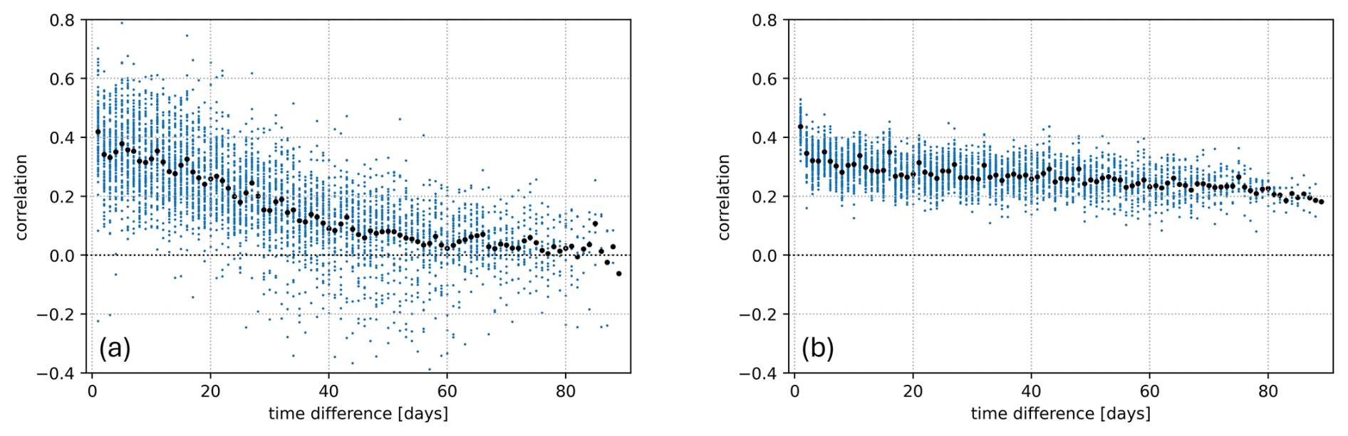
Figure 2 Temporal correlation in (a) difference of tropospheric NO₂ column for v2.3.1 and v2.4 for polluted areas (AMF uncertainty) and (b) observation forecast for unpolluted areas (stratospheric column uncertainty) between each combination of 2 d within the same month for the period 1 January–31 March 2019. Larger black points are the mean of correlations with the same time difference.

Next, we estimated temporal correlation factors for the stratospheric uncertainty. In the retrieval of the NO₂ columns, the observed slant column is split into its tropospheric and stratospheric parts using data assimilation in the TM5-MP model. We can assess uncertainty and bias in this model by investigating the difference between the forecasted column and the observed column (O–F) over unpolluted regions; see e.g. Dirksen et al. (2011). We take the values for O–F for the period 1 January to 31 March 2019. For each combination of 2 d within the same month, we determine the Pearson correlation coefficient in stratosphere O–F for clean areas (tropospheric vertical column $<\mathrm{0.6}\times {\mathrm{10}}^{\mathrm{15}}$ molecules cm⁻²) (Fig. 2b). This is again done with Eq. (12) but now with $\mathrm{\Delta }{N}_{t_{\mathrm{1}}}=N_{t_{\mathrm{1}}}^{\text{observation}}-N_{t_{\mathrm{1}}}^{\text{forecast}}$ and $\mathrm{\Delta }{N}_{t_{\mathrm{2}}}=N_{t_{\mathrm{2}}}^{\text{observation}}-N_{t_{\mathrm{2}}}^{\text{forecast}}$ the difference in stratospheric NO₂ between observation and forecast for the first day and second day respectively. For each “time difference” between daily O–F maps, we determine the mean correlation ($\stackrel{\mathrm{‾}}{r_{\mathrm{\Delta }t}}$). Then we take the mean of $\stackrel{\mathrm{‾}}{r_{\mathrm{\Delta }t}}$ for the time differences 1–30 d. This results in τ=0.30 for the NH winter period of 1 January to 31 March. The same method is carried out for the NH summer period 1 June–31 August, which showed a slightly lower correlation coefficient of τ=0.21. We take the higher value of ${\mathit{\tau }}_{N_{\mathrm{s}}^{\mathrm{strat}}}=\mathrm{0.30}$ as the temporal uncertainty correlation in the stratospheric uncertainty for both the NH winter and summer period, as a conservative uncertainty estimate. The correlation decreases slightly for longer periods and only disappears altogether for periods longer than 3 months.

The uncertainty in the slant column density is assumed to be fully uncorrelated in time (${\mathit{\tau }}_{N_{\mathrm{s}}}=\mathrm{0}$), following the same arguments as in the spatial uncertainty correlation (see Sect. 3.2.2).

The temporal correlation coefficient of the spatial representativeness uncertainty is set at fully random (τ_rs=0). The representativity can be correlated through time due to the effect of persistent cloud cover, but this will be assessed separately in the temporal representativeness uncertainty.

Table 2 Temporal error correlation sources and their random and systematic fractions for TROPOMI NO₂ tropospheric vertical column spatio-temporal averages.

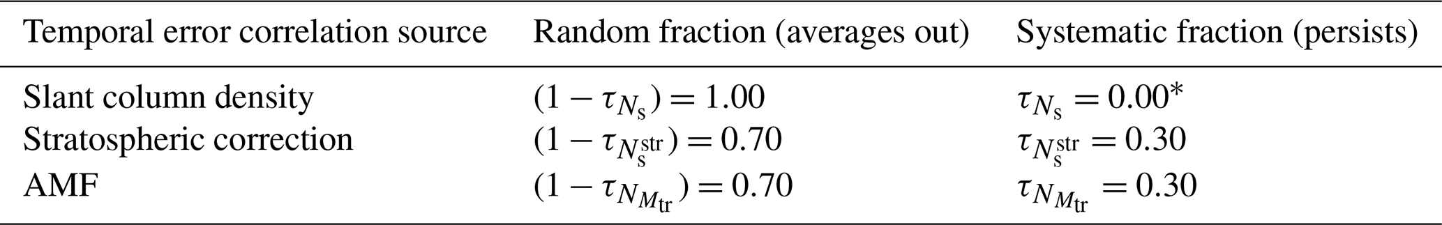
^∗ Note: the systematic component of the slant column density uncertainty is included in the stratospheric uncertainty.

The monthly mean L3 NO₂ columns are only representative when sufficient observations are available for calculating the means. The L3 qa_value (qa_L3 in the final data product – Table C1) is set to equal 1 when the data are representative as a monthly mean and equal 0 when it is not. This deviation is made using the count variable, which is the sum of the fractional coverages from the spatial averages α_o,t divided by the number of days in the month. If this value is below 0.1 (meaning less than 10 % of the month is sampled), the L3 qa_value (qa_L3) is set at 0, and the L3 NO₂ columns are advised not to be used for further analyses, as these would not be a good representation of the given month.

Temporal representativeness uncertainty

The temporal representativeness uncertainty (${\overline{\mathit{\sigma }}}_{\mathrm{rt}}$) can be interpreted as the standard error of the superobservations (spatial means) used to determine the monthly mean. We state that the number of possible observations within a month is finite, and a true monthly mean is obtained with at least one observation (note that the TROPOMI orbits overlap at higher latitudes, where multiple observations per day are possible) each day. A finite population correction is applied to the method of calculating the standard error to correct for this (Bondy and Zlot, 1976; Isserlis, 1918; Rijsdijk et al., 2025), resulting in the standard error decreasing to zero when observations are available for every day of the month. This results in the following theoretical formula for the temporal representativeness uncertainty:

$$\begin{array}{}\text{(13)}& {\overline{\mathit{\sigma }}}_{\mathrm{rt}}={\displaystyle \frac{{\mathit{\sigma }}_{x_{\mathrm{o},\mathrm{t}}}}{\sqrt{n}}}\sqrt{{\displaystyle \frac{N-n}{N-\mathrm{1}}}},\end{array}$$

where N is the length of the month in days and n is the number of days with at least one valid superobservation. The weighted standard deviation around the temporal mean ${\mathit{\sigma }}_{x_{\mathrm{o},\mathrm{t}}}$ is determined using

$$\begin{array}{}\text{(14)}& {\mathit{\sigma }}_{x_{\mathrm{o},\mathrm{t}}}=\sqrt{{\displaystyle \frac{{\sum }_{t=\mathrm{1}}^T\left(w_{\mathrm{o},\mathrm{t}}\right(x_{\mathrm{o},\mathrm{t}}-\overline{x}{)}^{\mathrm{2}})}{(T-\mathrm{1}){\sum }_{t=\mathrm{1}}^T{w}_{\mathrm{o},\mathrm{t}}}}},\end{array}$$

with T the total number of valid spatial averages in the period over which the averaging is performed, and $w_{\mathrm{o},\mathrm{t}}=\mathrm{1}-f$.

We apply the method also used in Rijsdijk et al. (2025) and Appendix B to assess whether Eq. (14) is suitable for assessing the temporal representativeness uncertainty. We start by taking a completely covered grid cell, which means that at least one spatial mean/superobservation was produced for this grid cell for every day of the month. The representativeness uncertainty can be quantified by comparing the mean of this completely covered grid cell to the mean of several samples (a subset of days) taken from that grid cell. We start by sampling a single day, which we use to estimate the temporal mean of the grid cell. Then we repeatedly add random days of the month and estimate the mean using the available observations. We perform multiple iterations (200) of this process on the same grid cell and find the relation between representativeness uncertainty f_t and temporal coverage of the grid cell (Fig. 3a). This process is then repeated for 100 grid cells in polluted areas (Fig. 3b). We only take polluted grid cells into account (mean NO₂ tropospheric vertical column of $\ge \mathrm{2}\times {\mathrm{10}}^{\mathrm{15}}$ molecules cm⁻²), as these are expected to have the highest temporal variability and thus are more likely to be sensitive to a sampling bias. The mean of the experiments (green) is almost identical to the theoretical solution of Eq. (13) (blue), showing that the formula is a suitable method for quantifying the temporal representativeness uncertainty for random sampling. Similar results are found for June 2019.

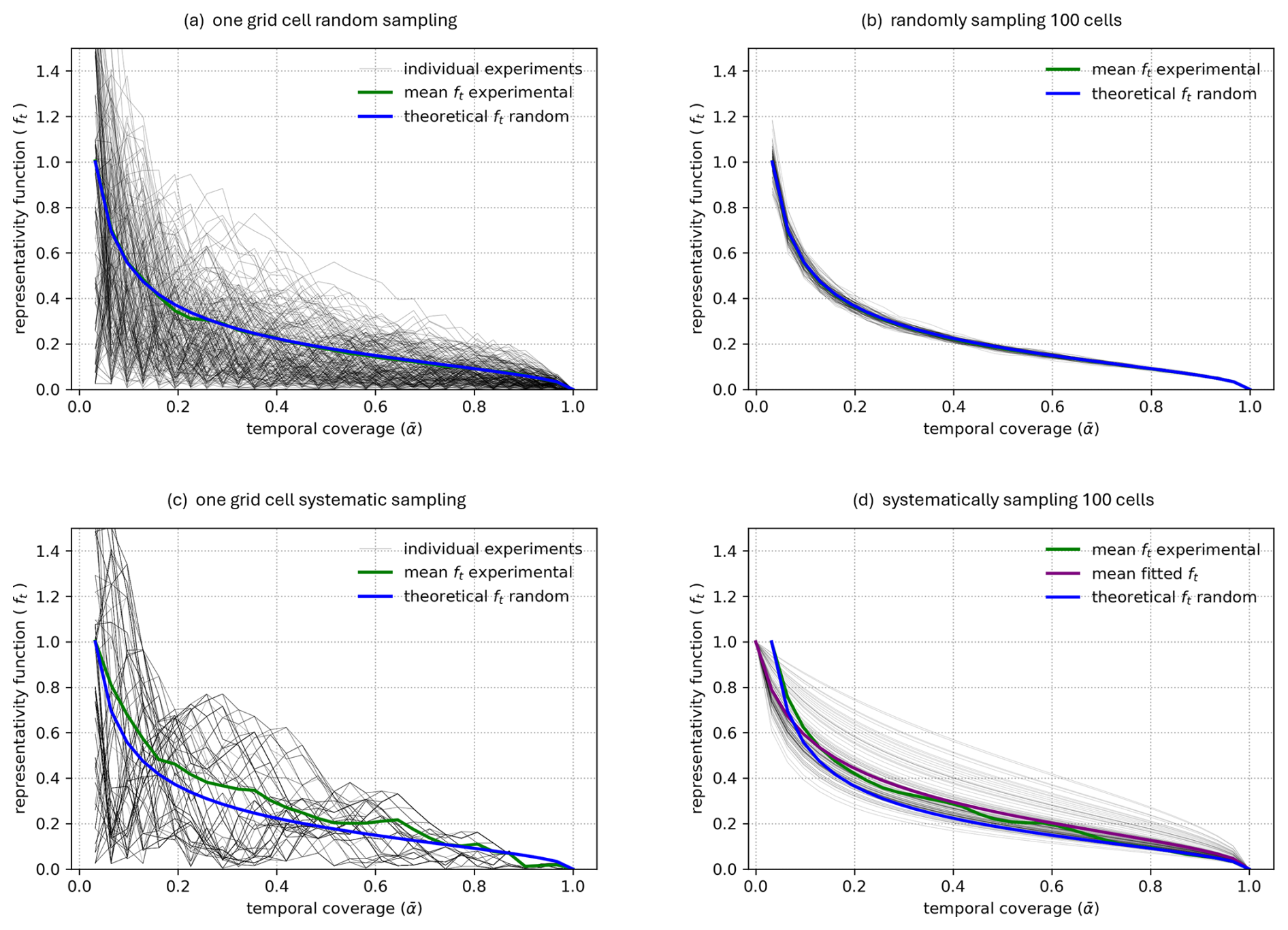
Figure 3 Results of repeatedly sampling grid cells to calculate ${\overline{\mathit{\sigma }}}_{\mathrm{rt}}$. (a) Repeated random sampling of 31 d of a single grid cell with values x_o,t. Daily observations in the grid cell are randomly sampled 200 times. The thin grey lines represent the difference between the sampled mean and the actual mean from individual random experiments. The green line is the mean of the samples and the blue line the theoretical result from Eq. (13). (b) Results of randomly sampling 100 grid cells. The grey lines are the green line from (a). The green line (overlapping the blue theoretical result) is the mean of the results of 100 grid cells. (c) Systematic sampling of a single grid cell. (d) Results of systematically sampling 100 grid cells. Observations in all panels are from January 2019 and have a mean tropospheric vertical column of $\ge \mathrm{2}\times {\mathrm{10}}^{\mathrm{15}}$ molecules cm⁻². Only grid cells with observation available every day are sampled.

As with the spatial representativeness (cloud masking one part of the grid cell), there might be a sensitivity to systematic sampling temporally. This could for example be the case if large weather systems gave persistent cloud cover in a given location for part of the month. The occurrence of systematic sampling was tested for the spatial means of January and June 2019. We selected grid cells in the spatial mean that had valid superobservations for ∼50 % of the given month. On these grid cells we applied a Wald–Wolfowitz test to determine whether the cloudiness was random or systematic (Wald and Wolfowitz, 1943). The Wald–Wolfowitz test is a non-parametric statistical test that checks a randomness hypothesis for a two-valued data sequence, in our case cloudy (no data) or non-cloudy (superobservation available, can be partly cloudy). For both January and June about two-thirds of the grid cells show systematic sampling due to continuous cloud cover for part of the month.

This shows that systematic sampling of observations for the temporal mean is relevant. Next, we will look into whether the temporal variability in the observations makes it sensitive to this systematic sampling. We repeat the method of repeated sampling of a grid cell as outlined above but now by sampling the grid cell systematically (start by taking the observation of 1 random day and then repeatedly add adjacent days). Figure 3d shows that systematic sampling produces more variability of grid cells around the theoretical solution (blue line, Eq. 13) than with random sampling (Fig. 3b) but that the mean of the experiments (green line) is close to the theoretical solution. Comparison with the spatial representativeness curve in Fig. B1b shows that the experimental curves in Fig. 3d are closer to the theoretical solution. The fit from Eq. (6) in purple does not show a better fit to the experimental mean than the theoretical solution does. This shows that the temporal mean is not very sensitive to systematic sampling, and the uncertainty can be assessed with the theoretical solution suggested in Eq. (13).

It should be noted that the sampling method can only be applied to grid cells that provide coverage for all days of the month. This is essentially only true for arid areas with almost no cloud cover. The question arises of how representative these regions are. We filter for relatively polluted regions ($\ge \mathrm{2}\times {\mathrm{10}}^{\mathrm{15}}$ molecules cm⁻²) and find more than 100 grid cells to which we can apply this method. These are found mostly in cities in the Middle East and western India, where January is in the dry season. We assume these polluted areas are representative of polluted areas in other parts of the world, and the theoretical solution can be applied globally.

4 TROPOMI NO₂ Level 3 dataset

4.1 Dataset

The here presented ESA CCI+ TROPOMI Level 3 dataset is available for the period May 2018 to December 2021 at a monthly resolution. The dataset is available on a global regular grid at different spatial resolutions: 0.2° × 0.2°, 0.5° × 0.5°, and 1° × 1°. The datasets are organised into a user-friendly and self-describing netCDF-4 format, following CF metadata conventions. The dataset represents the NO₂ columns at satellite overpass time (∼ 13:30 LT) under mostly clear-sky conditions.

The dataset contains both the tropospheric and stratospheric vertical column density (see Appendix C for all variables). The dataset contains two estimates of the total uncertainty for the tropospheric vertical column ${\overline{\mathit{\sigma }}}_{\mathrm{total}}$: one including the a priori uncertainty and one version excluding the a priori uncertainty, which can be used when applying the averaging kernel. A spatio-temporal average of the tropospheric averaging kernel from the L2 dataset is also available in the L3 dataset. For assessing the L3 data quality, the L3 qa_value, count variable, and average cloud radiance fraction are also available.

This dataset can be used for, for example, temporal analysis, emission monitoring, data assimilation and model validation, and atmospheric chemistry studies. It should be noted that this dataset is a clear-sky average, and model comparisons should only be done on cloud-free sampled model data, as previously recommended in Boersma et al. (2016). The cloud-free sampling of data causes biases with the true monthly mean in multiple ways. Firstly, photochemical reactions cause NO₂ to break down faster in clear-sky conditions (Miller et al., 1956), so the true monthly mean of tropospheric columns (when including vertical columns in overcast conditions) is higher by up to 25 % (Geddes et al., 2012; Boersma et al., 2016). Secondly, incident cloudiness over more or less polluted areas would cause uneven sampling, causing a bias either way. Lastly, cloudiness could be connected to atmospheric transport conditions that may bring clean or polluted conditions. The uncertainty assessment here represents the uncertainty of the L3 product to the clear-sky average and does not include an uncertainty to the true monthly mean.

4.2 Analysis of dataset

The results of the spatio-temporal average monthly mean and uncertainties for NO₂ for January and June 2019 are shown in Fig. 4, with local values given in Table 3. Missing data are mainly due to polar night at high latitudes and filtering of low-quality L2 data, due to, for example, consistent cloud or snow cover. All results presented in this section are from the 0.2° × 0.2° spatial resolution dataset.

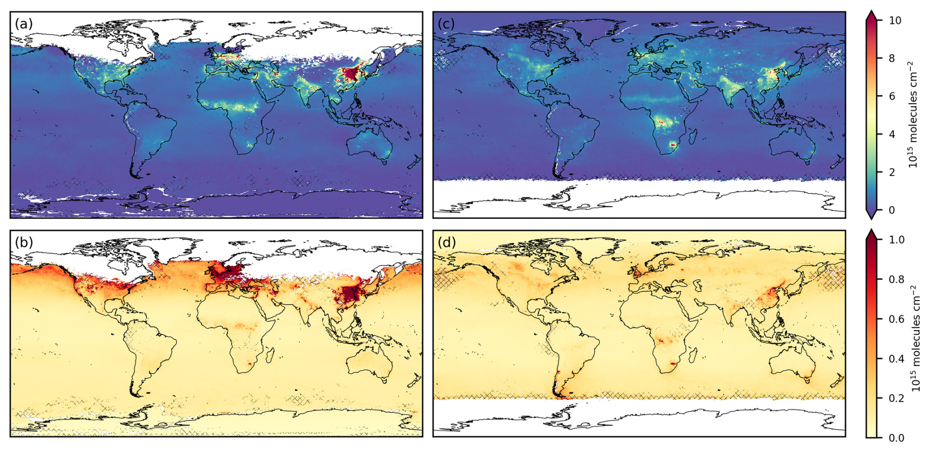
Figure 4 Example of results of the monthly (a) tropospheric NO₂ column with its (b) total uncertainty (${\overline{\mathit{\sigma }}}_{\mathrm{total}}$) for January 2019 and the same (c, d) for June 2019. Monthly means are calculated from individual L2 retrievals with good quality (qa_value = 0).

Table 3 Example values for monthly mean tropospheric NO₂ vertical column and uncertainties (with percentage of mean tropospheric vertical column) for a few selected locations for January and June 2019 (units: 10¹⁵ molecules cm⁻²). The values for Amsterdam, Beijing, and Rio de Janeiro were taken from one grid cell in the city centre location (52.3° N, 4.9° E for Amsterdam; 39.9° N, 116.3° E for Beijing; and 22.9° S, 43.1° W for Rio de Janeiro). The value for Africa biomass burning represents the location with the highest observed monthly mean value in the sub-equatorial region on the continent of Africa (in a box between latitudes 16° S and 16° N and longitudes 17.5° W and 42° E). The uncertainty estimates are with the a priori uncertainty, which does not need to be included when using the averaging kernel.

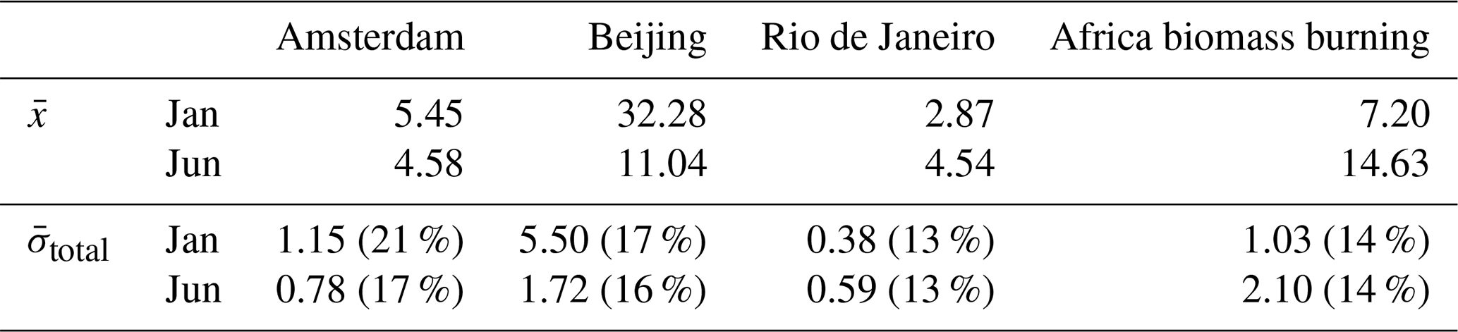
In June the tropospheric NO₂ columns are high in Africa due to wildfires and biomass burning in the dry season. In the urbanised areas in the Northern Hemisphere, tropospheric NO₂ columns have higher values during the winter season, reflecting longer lifetimes (e.g. Shah et al., 2020) and higher emissions due to heating, and thus we see higher values over Amsterdam and Beijing in January than in June (Table 3, Fig. 6). The opposite is true for urbanised areas in the Southern Hemisphere, for example Rio de Janeiro (Table 3, Fig. 6). The total uncertainty in winter when not applying the averaging kernel attributes to 21 % and 17 % of the total tropospheric vertical column for Amsterdam and Beijing respectively. These percentages are 19 % and 14 % respectively when applying the averaging kernel. Due to the averaging of random errors, the L3 uncertainty is lower than the uncertainty in L2 orbits, despite the introduction of representativeness errors. The average relative uncertainty in valid L2 pixels in January 2019 in Amsterdam is 52 %, compared to the 21 % in the L3 dataset. In Beijing the average relative L2 uncertainty is 28 %, compared to the 17 % in L3 in January 2019.

The separate uncertainty sources are shown in Fig. 5 for January 2019. Over unpolluted areas the largest source of uncertainty comes from the estimation of the stratospheric column concentration (Fig. 5b). In polluted regions the largest error source is the AMF uncertainty (Fig. 5c). Because the slant column density uncertainty is assumed random over both space and time, the uncertainty averages out over a large number of observations and is very small in the L3 dataset (Fig. 5a), but it should be noted that the systematic component of the slant column density uncertainty is included in the stratospheric uncertainty estimate. The spatial and temporal representativeness uncertainty is largest in Europe and East Asia, where the standard deviation of the tropospheric vertical column is largest but is a minor component in the total uncertainty budget.

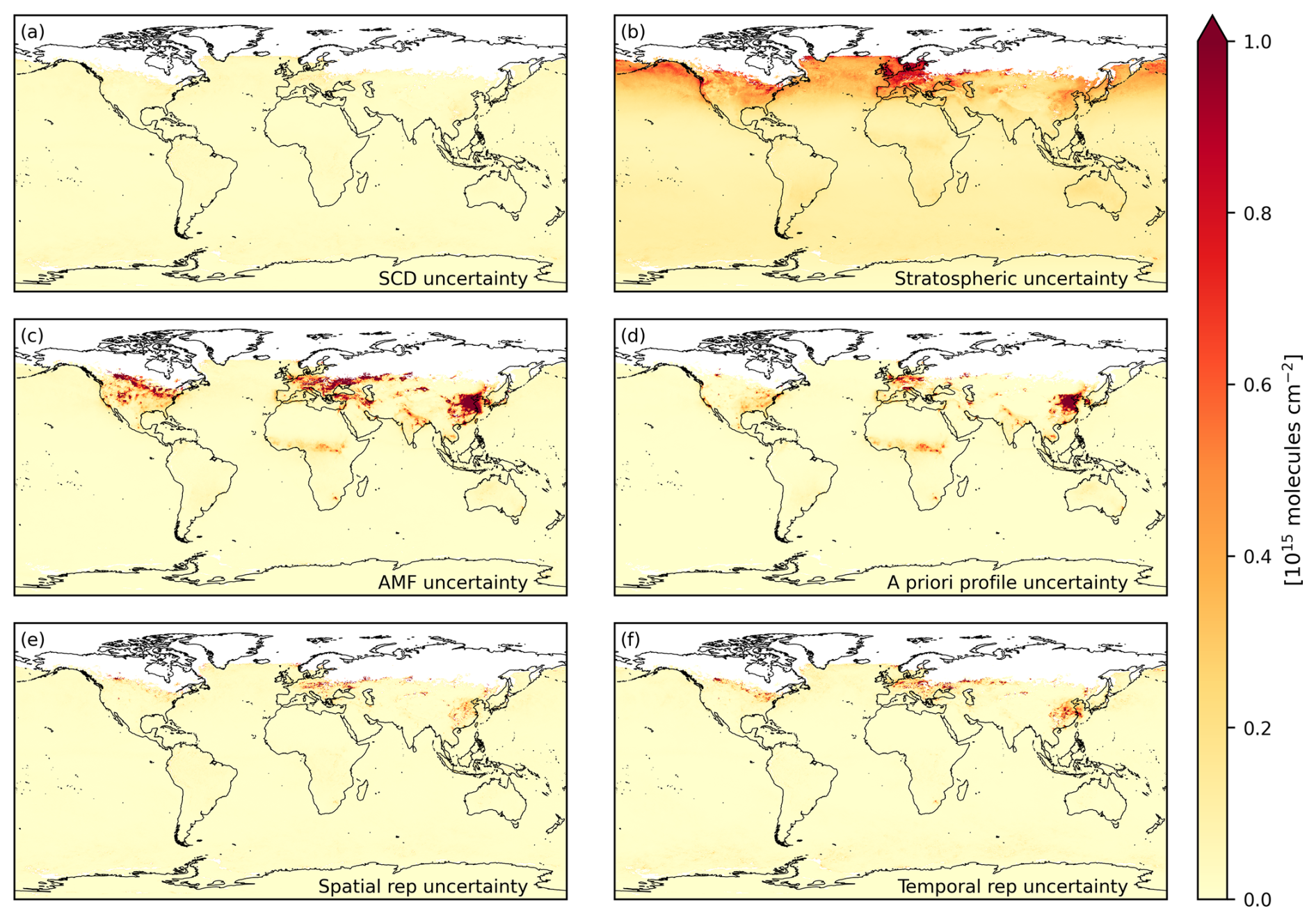
Figure 5 All components of tropospheric vertical column density uncertainty using the discussed spatial and temporal correlations for January 2019 (total uncertainty in Fig. 4b).

Time series of the tropospheric NO₂ column for four polluted locations are shown in Fig. 6. The available time series is too short to show long-term changes. The time series in Beijing and Amsterdam show features linked to the pandemic lockdowns (2020–2021) (Bauwens et al., 2020) and indicate an overall reduction of tropospheric NO₂ columns over the 5 years, although Amsterdam displays a large variability and the decrease may not be significant.

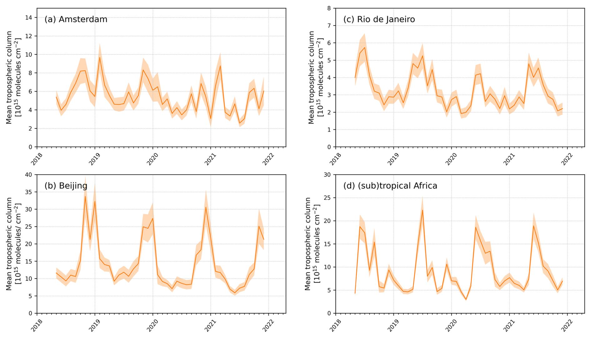
Figure 6 Time series of the monthly mean tropospheric vertical column NO₂ with the total uncertainty (${\overline{\mathit{\sigma }}}_{\mathrm{total}}$) for the same locations as in Table 3. The values in the time series represent a single L3 grid cell value, and the associated total uncertainty is given as the shaded area.

The Global Climate Observing System (GCOS) states requirements for observational datasets of the ECVs, including the precursors for aerosol and ozone variable NO₂ tropospheric vertical column (World Meteorological Organization (WMO) et al., 2022a). We examine the uncertainties in the NO₂ tropospheric vertical column against the GCOS-required measurement uncertainty (Fig. 7), which is formulated as a threshold, breakthrough, and goal value (World Meteorological Organization (WMO) et al., 2022b). The threshold requirement, the minimum requirement to be met to ensure that data are useful, requires the relative uncertainty to be lower than 100 % and the absolute uncertainty to be less than 5×10¹⁵ molecules cm⁻². The breakthrough requirement represents a significant improvement and requires the relative uncertainty to be lower than 40 % and the absolute uncertainty to be less than 2×10¹⁵ molecules cm⁻². Lastly, the goal is reached when the relative uncertainty is lower than 20 % and the absolute uncertainty is less than 1 × 10¹⁵ molecules cm⁻² (World Meteorological Organization (WMO) et al., 2022b). Due to the averaging of uncorrelated uncertainties in creating the L3 dataset, the GCOS requirements are met more frequently in L3 than in L2 (Fig. 7), suggesting L3 data are useful for climate monitoring. In June 2019 over Beijing the absolute uncertainty (as well as relative uncertainty) drops from an average of 2.81 × 10¹⁵ molecules cm⁻² (27.9 %) in L2, with most pixels reaching the threshold requirement, to 1.72 × 10¹⁵ molecules cm⁻² (15.5 %) in L3, well within the breakthrough requirement (Fig. 7c). Over Amsterdam the absolute uncertainty (as well as relative uncertainty) drops from an average of 1.44 × 10¹⁵ molecules cm⁻² (32.9 %) in L2, with most pixels reaching the breakthrough requirement, to 0.78 × 10¹⁵ molecules cm⁻² (16.9 %) in L3, within the goal requirement (Fig. 7d).

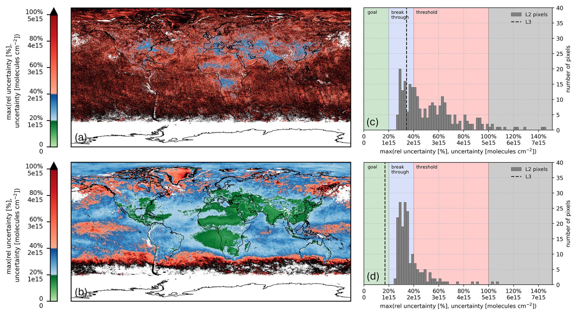
Figure 7 June 2019 (a) L2 and (b) L3 dataset as reviewed by the GCOS requirements for measurement uncertainty. Black regions do not fulfil the GCOS requirements, red regions fulfil “threshold” requirements, blue regions fulfil “breakthrough” requirements, and green regions fulfil “goal” requirements. The histograms show the L2 pixel uncertainties that fall into a single 0.2° × 0.2° L3 grid cell for (c) Beijing and (d) Amsterdam and the grid cell L3 total uncertainty (vertical line).

5 Validation

As independent validation, the ESA CCI+ TROPOMI Level 3 NO₂ dataset was compared to ground-based remote sensing measurements using the same reference data and methodologies used for the validation of the underlying Level-2 data reported in Verhoelst et al. (2021), in Van Geffen et al. (2022a), and in the S5P ATM-MPC quarterly Routine Operations Consolidated Validation Reports (ROCVR, available at https://mpc-vdaf.tropomi.eu/, last access: 30 August 2025). However, the monthly gridded nature of the L3 data does imply a need for some adaptations in the comparison methodology. The specific aspects and validation results are reported below, per (sub-)column. The L3 TROPOMI data were all filtered using the L3 qa_value (qa_L3).

5.1 Stratospheric slant column

The L3 TROPOMI stratospheric NO₂ columns were compared to the consolidated LATMOS_v3 sunset SAOZ measurements (Pommereau and Goutail, 1988) obtained at 10 sites covering mostly clean sites distributed globally from the southern high latitudes up to the northern high latitudes. These twilight zenith-sky measurements (Solomon et al., 1987) have an estimated uncertainty of about 10 %–14 % (Yela et al., 2017; Bognar et al., 2019), and they were adjusted to the average TROPOMI overpass time of the monthly averages (represented in the file as eff_frac_day) using a model-based photochemical adjustment (Hendrick et al., 2004). For optimal spatial co-location, we compared the SAOZ measurements to the TROPOMI 1.0 ° × 1.0° L3 grid cell covering the centre of the SAOZ observation. This procedure accounts for the large horizontal smoothing and offset in the SAOZ measurement sensitivity towards the setting sun (Lambert et al., 1997; Verhoelst et al., 2015). An illustration of such a comparison, at the Observatoire de Haute Provence in France, is shown in Fig. 8. This comparison shows excellent agreement, within the uncertainties of each product.

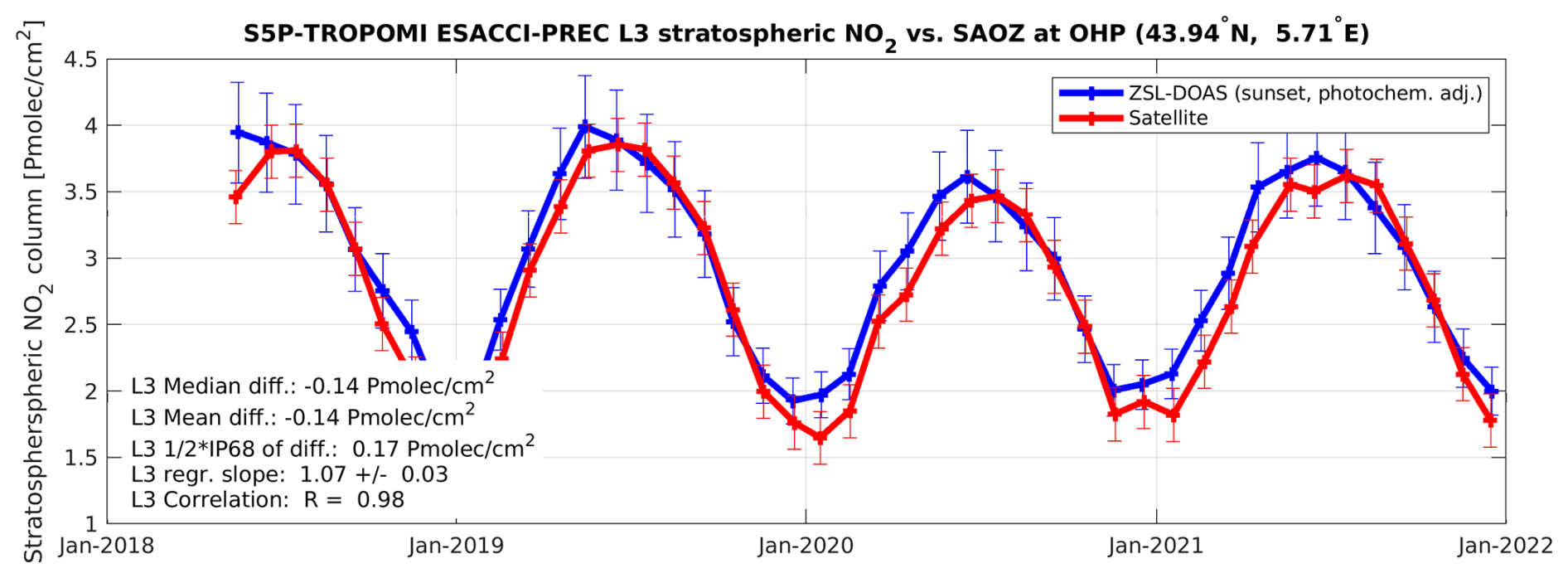
Figure 8 Time series of co-located L3 TROPOMI and photochemically adjusted sunset SAOZ stratospheric NO₂ column measurements at the Observatoire de Haute Provence (France).

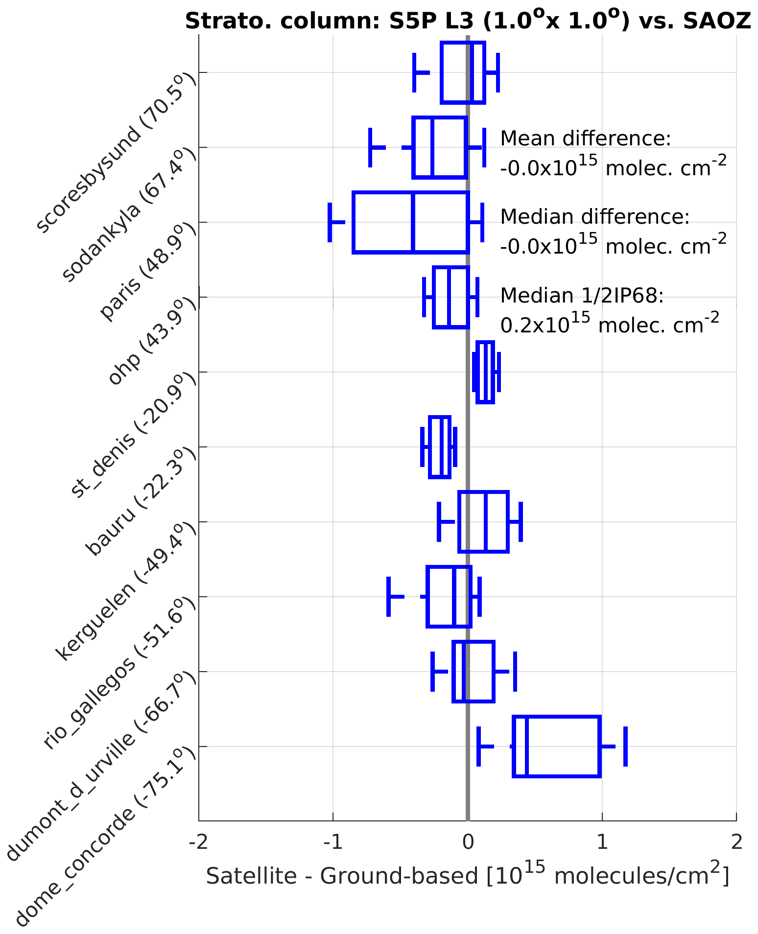
Figure 9 Box-and-whisker plots summarising from pole to pole the bias and spread of the difference between the L3 TROPOMI and ground-based SAOZ data (2018–2022). The median difference is represented by a vertical solid line inside the box that marks the 25 % and 75 % quantiles. The whiskers cover the 9 %–91 % range of the differences. Values between brackets in the labels denote the latitude of the station.

The network-wide results are summarised in Fig. 9. Overall, these stratospheric column comparisons yield results very similar to those for the underlying L2 (Verhoelst et al., 2021), with a virtually insignificant network-mean bias and a dispersion of typically around 0.2 × 10¹⁵ molecules cm⁻². The somewhat larger bias and dispersion over Paris is probably related to tropospheric contamination in the SAOZ measurements.

5.2 Tropospheric vertical column

The L3 TROPOMI tropospheric NO₂ vertical columns were compared to the MAX-DOAS tropospheric column data (Hönninger and Platt, 2002) collected from various sources and harmonised (in terms of file format) through the NIDFORVAL project for the operational S5P L2 validation. Total uncertainty estimates on these tropospheric vertical column density measurements are of the order of 7 %–17 % in polluted conditions, including both random (around 3 % to 10 %, depending on the instrument) and systematic (11 % to 14 %) contributions (e.g. Hendrick et al., 2014). MAX-DOAS data obtained within 30 min of the underlying L2 S5P data were compared to 0.2° × 0.2° L3 grid cells covering the station location. To ensure good temporal representativeness, only those sites at which at least a full year of comparisons could be made were retained. This yielded eight sites, covering moderately to severely polluted conditions. The most polluted case, Xianghe in China (e.g.  Pinardi et al., 2020), is analysed in Fig. 10, revealing a slightly better correlation and smaller dispersion of the differences than observed in the validation of the underlying L2 data. This is most likely due to the reduced measurement and atmospheric noise in the monthly averages. The mean and median difference are however more negatively biased, which can be attributed the poorer spatial resolution of the L3 dataset compared to the constituent L2 data. This is especially notable in the winter months, which due to pollution have high spatio-temporal variability in the L2 orbits and is smeared out in the averaging for the L3 data. There are also unresolved issues in wintertime MAX-DOAS retrievals done under very low viewing zenith angles in situations with thin boundary layers and high NO₂ concentrations, which could contribute to the bias (Cifuentes et al., 2025).

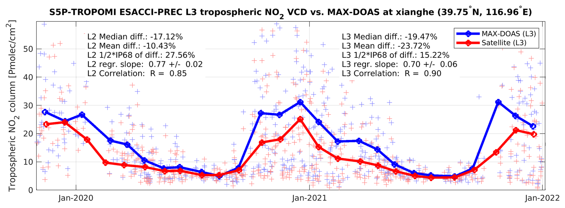
Figure 10 Time series of co-located TROPOMI and MAX-DOAS tropospheric NO₂ vertical column density (VCD) measurements at Xianghe (China). Light markers represent the co-located L2 data from the current operational processor (v2.4 RPRO, as used for ROCVR #24); the solid lines represent the L3 data.

The network-wide results for the MAX-DOAS comparisons are visualised in Fig. 11. These confirm the relatively small dispersion of the differences, typically about 12 %, which is well within the combined prognostic uncertainty budget (quadratic sum of 20 % uncertainty on the TROPOMI L3 data and probably at least 10 % on the monthly averaged MAX-DOAS data, depending on how one propagates the systematic and random components of the MAX-DOAS uncertainty). Also confirmed is the strong negative bias in TROPOMI NO₂, to be understood as a combination of the L2 negative bias and additional systematic differences related to the spatial smearing in the L3 data. Unexpected is the more pronounced negative bias at the relatively clean sites, which is opposite to the behaviour observed for the underlying L2 data. This result is not confirmed by the total column comparisons described in Sect. 5.3 and may be a case of small-number statistics or peculiarities at these individual sites.

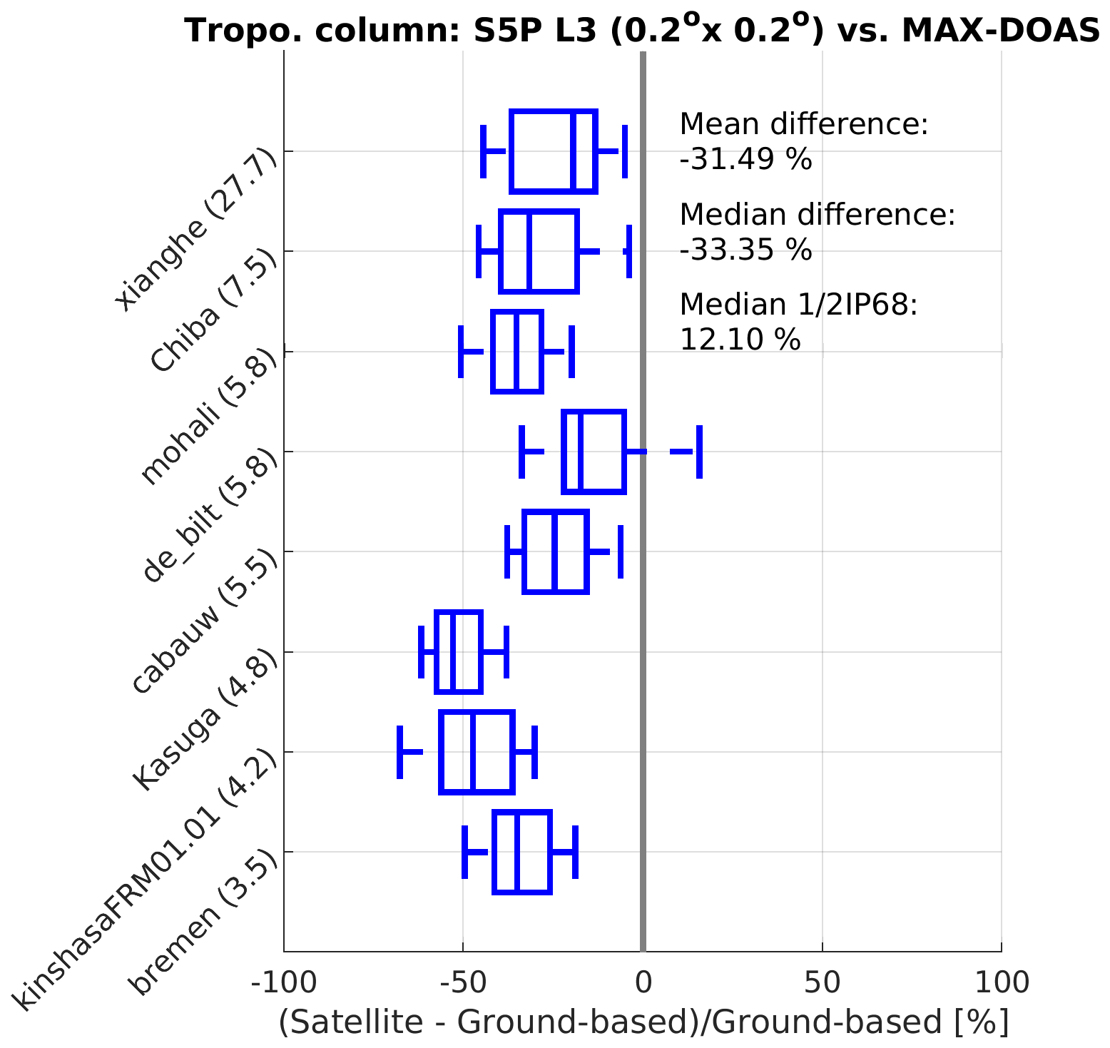
Figure 11 Similar to Fig. 9 but representing the agreement between the S5P-TROPOMI and MAX-DOAS tropospheric NO₂ column measurements, limited to those sites for which a full year of comparisons is available. Sites are ordered by mean tropospheric NO₂ vertical column density: cleaner sites at the bottom, more polluted sites at the top.

5.3 Total column

The TROPOMI L3 total NO₂ columns, calculated as the sum of the tropospheric and stratospheric vertical columns provided in the data files, were compared to Pandora direct-sun measurements (v1.8) from the Pandonia Global Network (PGN, https://pandonia-global-network.org/, last access: 30 August 2025). These measurements have a random error uncertainty of about 0.27×10¹⁵ molecules cm⁻² and a systematic error uncertainty of 2.7×10¹⁵ molecules cm⁻² (Herman et al., 2009). All Pandora measurements satisfying the recommended PGN quality filtering and obtained within 30 min from the satellite effective fractional day (eff_frac_day in the data files) were averaged, and only the 0.2° × 0.2° L3 grid cell covering the instrument location was used. To ensure good temporal representativeness, only those sites at which at least a full year of comparisons could be made were retained. This yielded eight sites, covering both unpolluted rural conditions and severe pollution, e.g. in the megacity of Mexico City. Figure 12 demonstrates the agreement at this most polluted site for both the L3 product and the current operational L2 product, which is the v2.4 full mission reprocessed (RPRO) dataset for this period of S5P measurements.

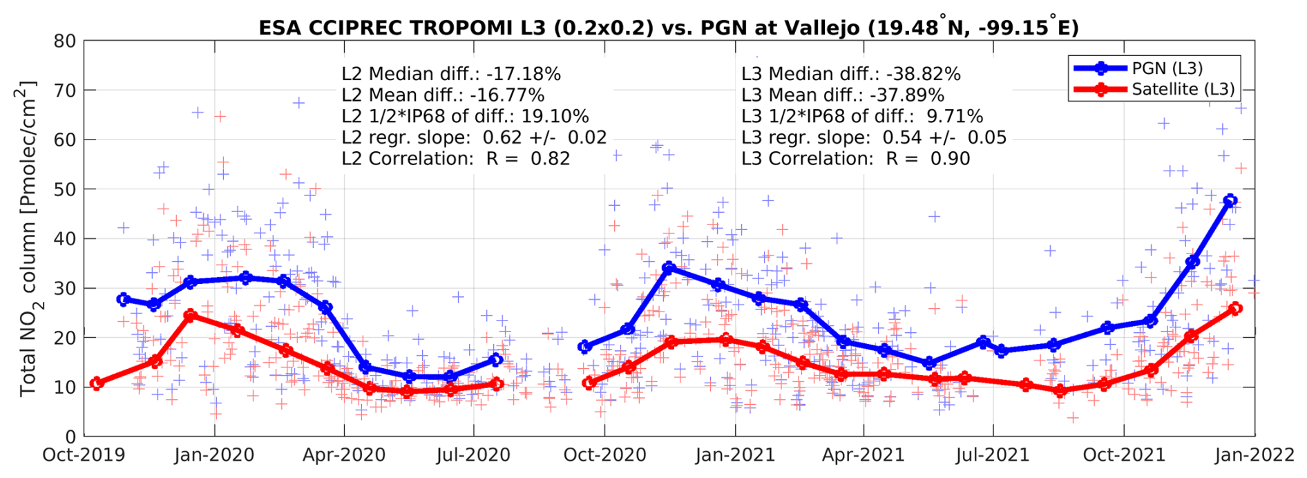
Figure 12 Time series of co-located TROPOMI and PGN total NO₂ column measurements at Vallejo (Mexico City). Light markers represent the co-located L2 data from the current operational processor (v2.4 RPRO, as available on the ATM-MPC VDAF AVS); the solid lines represent the L3 data.

As for the tropospheric vertical column density comparisons, the correlation between TROPOMI L3 and Pandora data is excellent (r∼0.9) for these comparisons in a highly polluted environment and even better than at L2. Again, as for the tropospheric column comparisons, the NO₂ underestimation already seen in L2 is more pronounced for the L3 NO₂ product with a median difference of about −39 % (versus −17 % for L2) and a regression slope of 0.54 (versus 0.62 for L2). For a pollution hot spot such as Mexico City, this is most likely due to the coarse L3 product resolution (0.2°), which tends to spatially smear out gradients compared to the pixel-resolution L2 data (0.05°). On the other hand, thanks to the temporal averaging, the dispersion of the differences between L3 and PANDORA NO₂ is significantly reduced, from nearly 20 % down to about 10 %. The network-wide results are summarised in Fig. 13. The tendency that TROPOMI NO₂ shows a more pronounced underestimation for larger total NO₂ column values is in line with the L2 validation results, which show virtually no underestimation (or even a very slight overestimation) at the cleanest sites, where the NO₂ column is dominated by the stratospheric contribution, and an underestimation up to 20 %–30 % at the most polluted sites (Verhoelst et al., 2021, and updates in the ROCVR). These total column results therefore do not confirm the more pronounced negative biases observed in the MAX-DOAS comparisons at sites with only moderate pollution (when compared to more polluted sites).

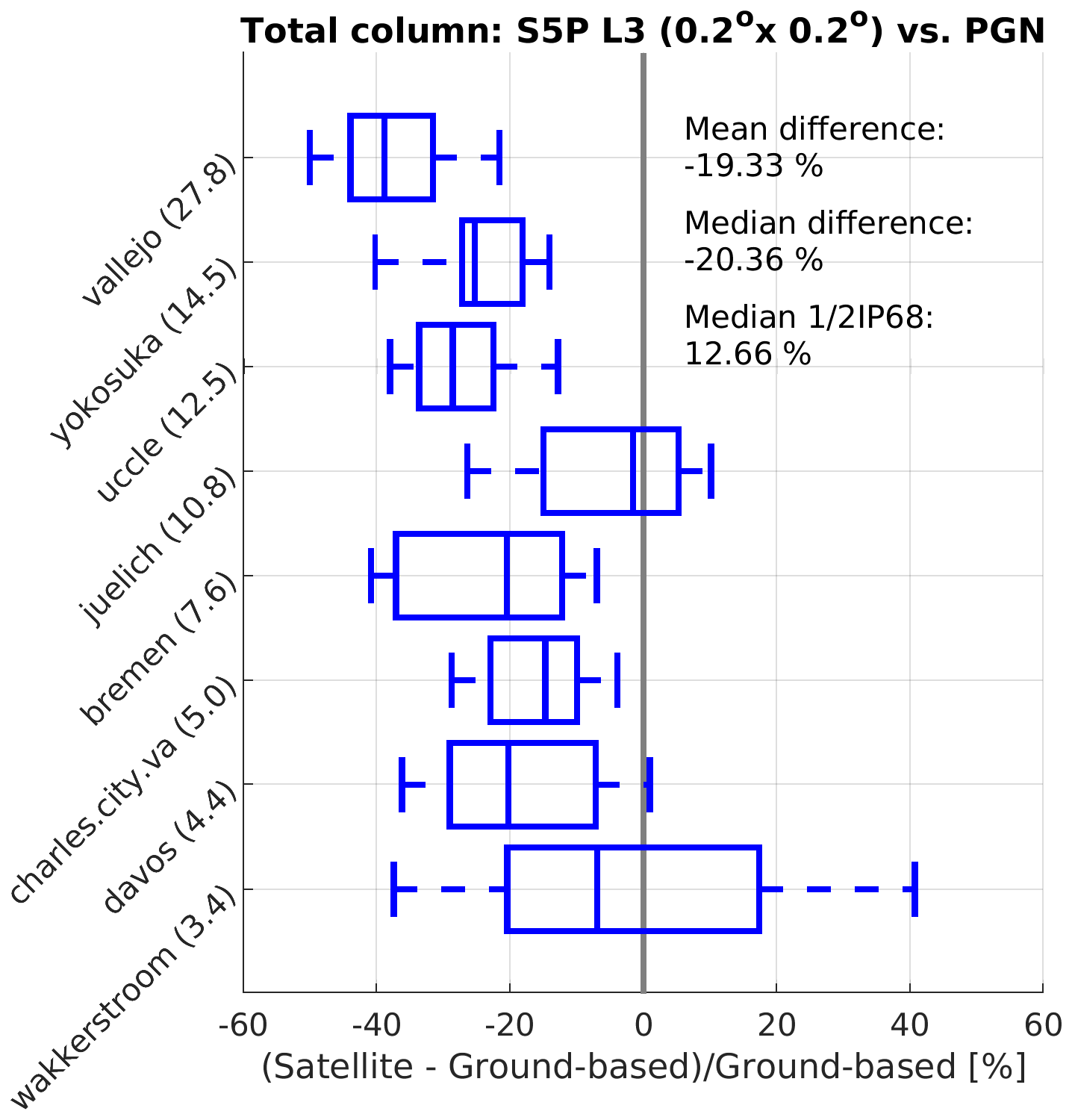
Figure 13 Similar to Fig. 9 but representing the agreement between the S5P-TROPOMI and PGN total NO₂ column measurements, limited to those sites for which a full year of comparisons is available. Sites are ordered by mean total NO₂ vertical column density: cleaner sites at the bottom, more polluted sites at the top.

6 Code and data availability

Data described in this article can be accessed at https://doi.org/10.21944/CCI-NO2-TROPOMI-L3 (KNMI, 2025). The generated L3 dataset will be made available on the ESA Climate Change Initiative Open Data portal. The software to create the spatial average is available at https://doi.org/10.5281/zenodo.10726644 (Rijsdijk and Eskes, 2024). Software to generate the temporal–spatial mean resulting in the L3 dataset is available at https://doi.org/10.5281/zenodo.14505524 (Glissenaar, 2024). The TROPOMI L2 v2.3.1 NO₂ dataset, which is the input for the generated dataset, is not the operational version and thus no longer publicly available. A sample of the data can be shared upon request. TROPOMI NO₂ L2 v2.4 is available on the Copernicus Data Space Ecosystem (https://doi.org/10.5270/S5P-9bnp8q8, Copernicus Sentinel-5P, 2021b). The reference data used for the ground-based validation are available from the NDACC Data Host Facility at https://ndacc.larc.nasa.gov/ (NDACC, 2025) (SAOZ and selected MAX-DOAS data) and from both the PGN website (https://www.pandonia-global-network.org/, Pandonia Global Network (PGN), 2025) and ESA's Validation Data Center (ESA Validation Data Center (EVDC), 2025, https://evdc.esa.int/) for the Pandora data.

7 Conclusions

We developed a comprehensive Level 3 (L3) dataset of gridded and averaged tropospheric NO₂ column retrievals (v2.3.1) from the TROPOMI sensor, covering the period from May 2018 to December 2021. The dataset is available at multiple spatial resolutions (0.2° × 0.2°, 0.5° × 0.5°, and 1° × 1°) on a monthly timescale. Using a tiling (superobservation) approach, we ensured that (1) valid NO₂ retrievals are gridded according to pixel area, and (2) temporal averages are calculated as weighted means, with weights reflecting the representativeness of superobservations for specific days. This L3 dataset is applicable for clear-sky or low-cloud-fraction conditions at TROPOMI's overpass time of 13:30 LT.

Realistic uncertainties were derived by propagating L2 retrieval uncertainties. To address spatial and temporal error correlations, we considered errors in the stratosphere–troposphere separation and air mass factor calculations, which are partly spatially correlated. Representativeness uncertainty, stemming from incomplete coverage of grid cells by valid L2 retrievals (e.g. due to cloud cover), was found to be more significant in polluted regions. The combined L3 uncertainty accounts for both measurement uncertainties (including spatial representativeness errors) and temporal representativeness uncertainties. An analysis showed that 30 % of retrieval uncertainties persist over a month due to error correlations in the stratosphere–troposphere separation and air mass factor calculations.

Over polluted areas, the L3 dataset showed reduced uncertainties compared to averaged L2 retrievals, demonstrating the effectiveness of averaging large numbers of observations. For example, while monthly average L2 uncertainties are 30 %–50 % over Beijing and Amsterdam, they drop to 20 % or less in the L3 dataset, meeting the GCOS “breakthrough” and even “goal” requirements. Validation against ground-based PANDORA measurements revealed a consistent temporal correlation but with a low bias of 20 %, partly attributed to more pronounced spatial smearing in the L3 product.

This monthly mean L3 TROPOMI tropospheric NO₂ dataset offers a coherent and much-reduced (in size) data record, making it suitable for atmospheric chemistry studies, for evaluating atmospheric models, and for analysing spatiotemporal NO₂ trends. The methods presented here can be replicated when creating L3 datasets for other atmospheric gases and other Earth observation L3 datasets. Future work will include applying the presented methods on NO₂ retrievals from OMI and combine TROPOMI and OMI observations to create a decades-long consistent CDR.

Appendix A: L2 observations in the descending node

During polar summer, the polar regions are marked by 24 h daylight. In the Northern Hemisphere, this means that the polar region on the “backside” of the Earth is experiencing daylight from May to August, and observations are made in the descending node of the satellite. These observations in the descending node are included in the L2 NO₂ product and not quality-flagged in the qa_value before version 2.7.

However, we find that the observations in the descending node of the orbit show structurally different retrieval results for the tropospheric vertical NO₂ column in the Arctic region (north of 60° latitude) than the observations from the ascending node in June (Fig. A1a). While retrievals in the ascending part of the orbit show a median value of 0.2 × 10 molecules cm⁻², retrievals in the descending part show a long tail of negative tropospheric NO₂ values, and the mode of the probability density curve is negative. This difference between results from the ascending and descending part of the orbits is less obvious in the Antarctic region in December (Fig. A1b).

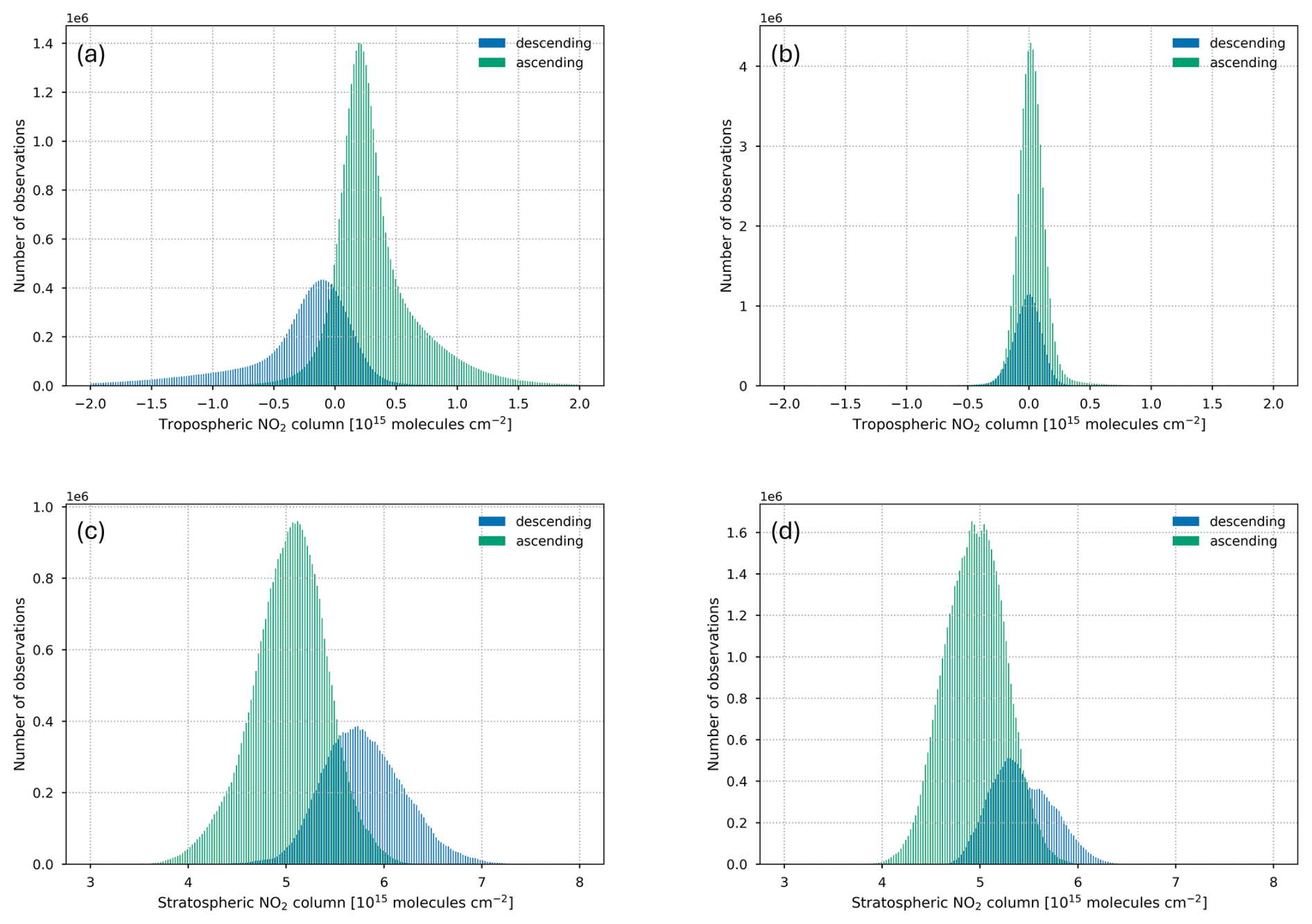
Figure A1 NO₂ vertical column observations (qa_value > 0.75) in ascending and descending mode for the troposphere (a) and stratosphere (c) north of 60° latitude from orbits in June 2019 and for the troposphere (b) and stratosphere (d) south of −60° latitude from orbits in December 2019.

A TROPOMI validation report (Lambert et al., 2023) has shown that TROPOMI underestimates tropospheric NO₂ columns compared to ground-based Pandora instruments at the high-latitude locations of Ny-Ålesund and Eureka by about 15 %. The discrepancy between tropospheric NO₂ column observations from the descending node and ascending node could play a role in this underestimation.

The discrepancy between retrievals done in the descending and ascending node is caused because the descending node observations are not included in the data assimilation in TM5-MP, and thus the stratospheric columns are more uncertain and often overestimated (Fig. A1c). Based on these results, we recommend to not use retrievals from the descending part of the orbit. From TROPOMI L2 version 2.7 onwards, the qa_value is adjusted to include flags for the descending orbital observations.

Appendix B: The number of effective observations

The number of effective observations N_eff characterises how sensitive a region is to systematic sampling, which can occur due to for example a cloud field covering part of a grid cell. The lower the value for N_eff, the more sensitive a region is to systematic sampling. In a region where the uncertainty in NO₂ columns is dominated by noise, usually a relatively unpolluted region, the N_eff is high. In such a region, the draw of one retrieval can be enough to characterise the spatial ensemble on a whole. In an area with strong pollution gradients, usually a polluted area, multiple draws are needed for proper characterisation. For example, a grid cell covering a city effectively consists of two types of NO₂ observations: those over the polluted city and those over the unpolluted nearby rural area, and such areas are thus sensitive to systematic sampling.

The value for N_eff was estimated by Rijsdijk et al. (2025) by repeatedly sampling a fully covered grid cell in a systematic way (starting with one random pixel and then adding neighbouring pixels) and calculating the representativeness (the absolute difference between the mean of observed pixels and the true mean of the fully covered grid cell when including all pixels). The representativeness function f in Eq. (6) was then fitted to the mean of these experiments, providing the number of effective observations N_eff for this superobservation grid cell (Fig. B1a). For this polluted grid cell, with resolution 0.2° × 0.2° and TROPOMI pixels of 5.5 × 3.5 km², the number of effective observations N_eff is somewhat smaller than 13.

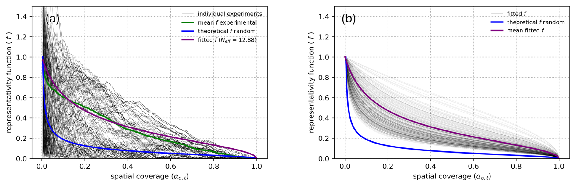
Figure B1 Results of repeatedly sampling grid cells in a systematic way to calculate the representativeness function f. (a) One single grid cell (polluted, $x_{\mathrm{o},\mathrm{t}}\ge \mathrm{1.8}$× 10¹⁵ molecules cm⁻²) sampled 200 times. The grey lines represent 200 individual experiments sampling the same superobservation grid cell. The green line is the mean of the individual experiments, and the purple curve is the representativeness function in Eq. (6) fitted to the green line. The blue curve shows the theoretical representativeness function in the case of random sampling (result if grid cell is not sensitive to systematic sampling). (b) Results of sampling 100 grid cells in polluted regions. The grey lines are a collection of purple lines from (a); the purple curve is the mean of the grey curves. The blue line again shows the theoretical random solution.

Table B1 The ratio $N/N_{\mathrm{eff}}$ for TROPOMI NO₂ in unpolluted and polluted ($x_{\mathrm{o},\mathrm{t}}>\mathrm{1.8}\times {\mathrm{10}}^{\mathrm{15}}$ molecules cm⁻²) regions for different spatial resolutions of the superobservation grid. The ratio increases with superobservation area (°²).

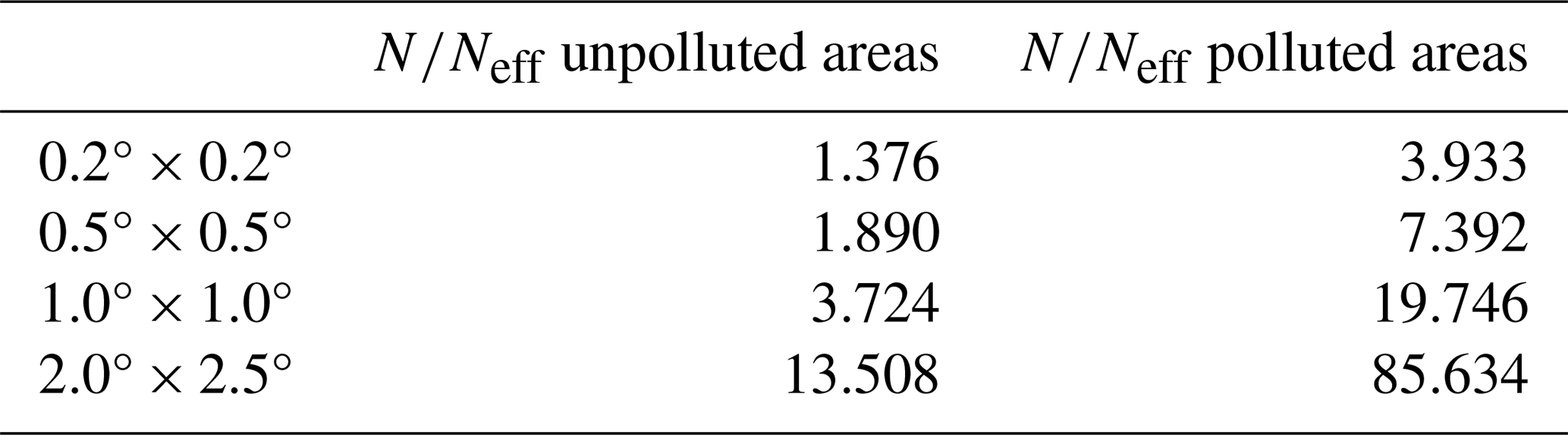
This method was repeated for multiple superobservation grid cells. The results showed that polluted regions ($x_{\mathrm{o},\mathrm{t}}\ge \mathrm{1.8}$ molecules cm⁻²) have a lower value for N_eff than unpolluted regions ($x_{\mathrm{o},\mathrm{t}}<\mathrm{1.8}$ molecules cm⁻²), making it more sensitive to systematic sampling (Rijsdijk et al., 2025). The ratio $N/N_{\mathrm{eff}}$, where N is the number of pixels (valid or not) in a superobservation, was determined for NO₂ retrievals from TROPOMI in Rijsdijk et al. (2025) to be linearly dependent on the grid resolution. This linear relationship was determined for both polluted and unpolluted superobservations by Rijsdijk et al. (2025). For a superobservation resolution of 0.2° × 0.2°, this results in $N/N_{\mathrm{eff}}=\mathrm{1.376}$ for unpolluted areas which are not sensitive to systematic sampling and $N/N_{\mathrm{eff}}=\mathrm{3.933}$ for polluted areas which are more sensitive to systematic sampling (Table B1). These ratios are used to determine the number of effective observations N_eff for each grid cell in the superobservation. When the N_eff is equal to the number of pixels N, and thus the ratio $N/N_{\mathrm{eff}}$ equals 1, systematic sampling has no effect. The ratios $N/N_{\mathrm{eff}}$ would need to be redetermined for another substance or sensor (with a different pixel resolution) following the methods in Rijsdijk et al. (2025).

Appendix C: Contents of L3 dataset

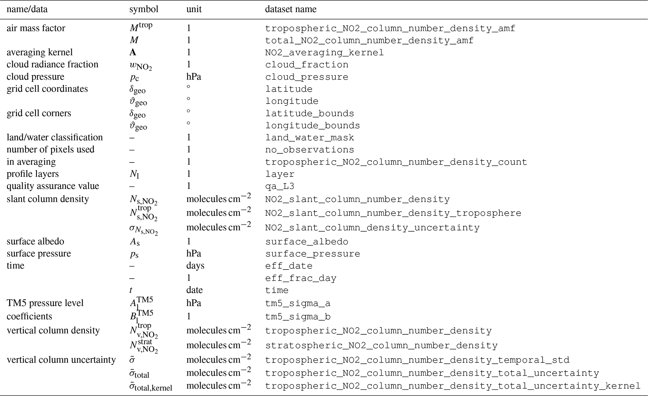
Table C1 Overview of the variables, units, and types in the main L3 data output product file.