A hyperspectral and multi-angular synthetic dataset for algorithm development in waters of varying trophic levels and optical complexity

This data paper outlines the development and the structure of a new synthetic dataset within an extended optical domain, encompassing inherent and apparent optical properties (IOPs and AOPs) alongside associated optically active constituents (OACs). Bio-optical modeling benefited from knowledge and data accumulated over the past 3 decades, enabling the imposition of rigorous quality standards and the definition of novel bio-optical relationships that are significant contributions on their own. Employing the HydroLight scalar radiative transfer equation solver, above-surface and submarine light fields between 350 and 800 nm at 1 nm steps were generated, facilitating algorithm development and assessment for present and forthcoming hyperspectral satellite missions. A smaller version of the dataset, delivered at 12 Sentinel-3 Ocean and Land Colour Instrument (OLCI) bands (400 to 753 nm), was also produced, targeting multispectral sensor algorithm research. Derived AOPs encompass an array of above- and below-surface reflectances, diffuse attenuation coefficients, average cosines, and Q factor. The dataset is distributed in 5000 files, each encapsulating a specific IOP scenario, ensuring sufficient data volume for each represented water type. AOPs are resolved across the complete range of solar and viewing zenith and azimuthal angles as per the HydroLight default quadrants, amounting to 1300 angular combinations. This comprehensive directional coverage caters to studies investigating signal directionality, which previously lacked sufficient reference data. The dataset is publicly available for anonymous retrieval via the FAIR repository Zenodo at https://doi.org/10.5281/zenodo.11637178 (Pitarch and Brando, 2024).

1 Introduction and review

1.1 Background

Marine optics studies the light that is measured by optical radiometers both in the water or above the surface. The optical signal is conveniently formulated in terms of apparent optical properties (AOPs), which are normalized quantities less dependent on the intensity of the incident light than the radiances or irradiances from which they originate. The most notable AOP is the remote-sensing reflectance (R_rs), defined as the water-leaving radiance (L_w) per unit of above-water planar downwelling irradiance (E_s), retrievable from satellite observations after atmospheric correction. Other quantities like diffuse attenuation coefficients, average cosines, and the Q factor find applications in marine optics too (Mobley, 1994).

AOPs are linked to the optically active water constituents (OACs), which are commonly phytoplankton and other suspended and dissolved substances. Phytoplankton is typically quantified in terms of the chlorophyll concentration (C), and non-living solids suspended in the water can be grouped in the non-algal particles (NAP), quantified by their concentration (N), though different splits of the particulate material are possible, such as particles of organic and inorganic origin. Dissolved substances, optically categorized as colored dissolved organic matter (CDOM), are not commonly given in terms of mass concentration units but in terms of the absorption coefficient spectrum, commonly at 440 nm (Y or a_g(440)).

Empirical algorithms can be developed to invert any of the OACs from measured AOPs by finding statistical relationships between matched AOP and OAC data (IOCCG, 2006). This approach, although sometimes operationally robust and mechanistically meaningful, hampers progress in understanding the optical influence of OACs, which is given by the inherent optical properties (IOPs) – namely, the absorption and scattering coefficients. The IOPs can be mathematically linked to the OACs with the so-called bio-optical relationships and to the AOPs through the radiative transfer equation, hence making it a mathematical bridge between the AOPs and the OACs (Mobley, 1994).

The OACs are the independent variables that drive the generation of a synthetic dataset (SD). They can be a single quantity like C (IOCCG, 2006; Loisel et al., 2023), typically chosen for open sea conditions, or a triplet formed by C, N, and Y (Nechad et al., 2015) or another combination, which is a usual choice for optically complex waters. More variables give more flexibility, but bio-optical relationships must be established for all of them to derive the IOPs. Statistical relationships between C and IOPs have been studied for decades (Bricaud et al., 1998; Loisel and Morel, 1998; Morel and Maritorena, 2001). Much less is known about N and Y, particularly in optically complex waters, where their bio-optical properties are much more regionally variable. Nevertheless, in the last 2 decades, fractional information on Australian waters (Blondeau-Patissier et al., 2009; Cherukuru et al., 2016; Blondeau-Patissier et al., 2017), European waters (Tilstone et al., 2012; Martinez-Vicente et al., 2010; Astoreca et al., 2012), South African lakes (Matthews and Bernard, 2013), North American coastal waters (Aurin et al., 2010; Le et al., 2013, 2015), and other localized areas have contributed to a significant increase in the understanding of the bio-optics in optically complex waters.

Assuming an unpolarized submarine light field, IOPs consist of the absorption coefficient (a) dependent on the wavelength (λ) and the volume scattering function (VSF; symbol β), which can be broken down to the contribution of single OACs. For the setup used in this SD, consisting of phytoplankton, NAP, and dissolved matter, the IOPs break down as in Eq. (1), which includes the contribution by seawater itself and assumes that dissolved material does not significantly scatter light in the optical domain:

$$\begin{array}{}\text{(1)}& \left\{\begin{array}{l}a\left(\mathit{\lambda }\right)=a_{\mathrm{w}}\left(\mathit{\lambda }\right)+a_{\mathrm{ph}}\left(\mathit{\lambda }\right)+a_{\mathrm{NAP}}\left(\mathit{\lambda }\right)+a_{\mathrm{g}}\left(\mathit{\lambda }\right),\\ \mathit{\beta }\left(\mathrm{\Psi },\mathit{\lambda }\right)={\mathit{\beta }}_{\mathrm{w}}\left(\mathrm{\Psi },\mathit{\lambda }\right)+{\mathit{\beta }}_{\mathrm{ph}}\left(\mathrm{\Psi },\mathit{\lambda }\right)+{\mathit{\beta }}_{\mathrm{NAP}}\left(\mathrm{\Psi },\mathit{\lambda }\right).\end{array}\right.\end{array}$$

For radiative transfer purposes, it is the total absorption coefficient, a, that is the relevant quantity. Instead, the VSF is resolved as a function of the scattering angle (Ψ). This creates a varying balance of the single contributors to scattering as their respective variabilities with Ψ are different. Specifically, the strongest differences are between water and other particulate materials.

Because of the technical difficulties in measuring angularly resolved scattering, optical theory deals mostly with angular integrals of the VSF that are much more commonly measured with commercial instrumentation. If the VSF is integrated across the backward hemisphere, one obtains the backscattering coefficient (b_b), whereas if one integrates across all directions, one obtains the scattering coefficient (b). The total light attenuation along a direction is quantified with the beam attenuation coefficient ($c=a+b$). c is arguably the most measured IOP in all of optics' history, and its bio-optics has been studied for many decades as opposed to b and especially b_b, the measurements of which are much scarcer and more recent. c keeps the same additive property for each constituent. Hence, Eq. (2) applies:

$$\begin{array}{}\text{(2)}& \left\{\begin{array}{l}{b}_{\mathrm{b}}\left(\mathit{\lambda }\right)=b_{\mathrm{bw}}\left(\mathit{\lambda }\right)+b_{\mathrm{b},\mathrm{ph}}\left(\mathit{\lambda }\right)+b_{\mathrm{b},\mathrm{NAP}}\left(\mathit{\lambda }\right),\\ b\left(\mathit{\lambda }\right)=b_{\mathrm{w}}\left(\mathit{\lambda }\right)+b_{\mathrm{ph}}\left(\mathit{\lambda }\right)+b_{\mathrm{NAP}}\left(\mathit{\lambda }\right),\\ c\left(\mathit{\lambda }\right)=c_{\mathrm{w}}\left(\mathit{\lambda }\right)+c_{\mathrm{ph}}\left(\mathit{\lambda }\right)+c_{\mathrm{NAP}}\left(\mathit{\lambda }\right)+a_{\mathrm{g}}\left(\mathit{\lambda }\right).\end{array}\right.\end{array}$$

Given a certain constituent, whether phytoplankton or NAP, its VSF is normalized by its scattering coefficient to obtain the phase function (PF) as in Eq. (3):

$$\begin{array}{}\text{(3)}& {\stackrel{\mathrm{̃}}{\mathit{\beta }}}_x={\displaystyle \frac{{\mathit{\beta }}_x}{b_x}},x=\text{ph}\text{ or NAP}.\end{array}$$

This normalization removes the variation in scale due to particle concentration so that the PF is a specific characteristic of the given particle type. For radiative transfer calculations, the PF must be set a priori for each OAC. That can be a measured phase function (He et al., 2017) but is more commonly from a family of simulated functions after electromagnetic scattering calculations (Morel et al., 2002; Fournier and Forand, 1994). For the latter case in particular, Mobley et al. (2002) arranged an mathematical equation to select one PF from the Fournier–Forand PF family given the backscattering ratio, defined as in Eq. (4):

$$\begin{array}{}\text{(4)}& B_x={\displaystyle \frac{b_{\mathrm{b},x}}{b_x}},x=\text{ph}\text{ or NAP}.\end{array}$$

Despite the fact that the bio-optical modeling for this SD considers the separate phytoplanktonic and non-algal parts individually, their scattering and attenuation coefficients cannot be measured separately Instead, there is literature on bio-optical relationships involving their “particle” aggregates as in Eq. (5):

$$\begin{array}{}\text{(5)}& \left\{\begin{array}{l}{b}_{\mathrm{bp}}\left(\mathit{\lambda }\right)=b_{\mathrm{b},\mathrm{ph}}\left(\mathit{\lambda }\right)+b_{\mathrm{b},\mathrm{NAP}}\left(\mathit{\lambda }\right),\\ b_p\left(\mathit{\lambda }\right)=b_{\mathrm{ph}}\left(\mathit{\lambda }\right)+b_{\mathrm{NAP}}\left(\mathit{\lambda }\right),\\ c_p\left(\mathit{\lambda }\right)=c_{\mathrm{ph}}\left(\mathit{\lambda }\right)+c_{\mathrm{NAP}}\left(\mathit{\lambda }\right).\end{array}\right.\end{array}$$

Bulk absorption and attenuation are also commonly measured and, after removing the water baselines, become the “non-water” components as in Eq. (6):

$$\begin{array}{}\text{(6)}& \left\{\begin{array}{l}{a}_{\mathrm{nw}}\left(\mathit{\lambda }\right)=a_{\mathrm{ph}}\left(\mathit{\lambda }\right)+a_{\mathrm{NAP}}\left(\mathit{\lambda }\right)+a_{\mathrm{g}}\left(\mathit{\lambda }\right),\\ c_{\mathrm{nw}}\left(\mathit{\lambda }\right)=c_{\mathrm{ph}}\left(\mathit{\lambda }\right)+c_{\mathrm{NAP}}\left(\mathit{\lambda }\right)+c_{\mathrm{g}}\left(\mathit{\lambda }\right).\end{array}\right.\end{array}$$

In order to develop updated bio-optical relationships and remote-sensing algorithms, there is a need for large concomitant OAC–IOP–AOP datasets across a range of data values, seasons, and geographical locations, with fully characterized uncertainties. However, despite broader accessibility of field- and laboratory-based IOP instrumentation, current data availability and quality are below what was expected 25 years ago, when instrumentation became commercially available. Open-access OAC–IOP–AOP datasets are scarce, strongly concentrated in some areas, and without characterized uncertainties. Given this absence of data, it has been a common choice to develop SDs for optical studies (IOCCG, 2006; Nechad et al., 2015; Loisel et al., 2023). Their IOP–AOP relationships can be considered error-free as they are derived from the solution of the radiative transfer equation, yet this exact relationship does not confer validity to the SD per se as the IOPs resulting from bio-optical modeling could be unrealistic. SDs have a history of applications to the development of algorithms of varying complexity, from semi-analytical algorithms (Lee et al., 2002) to complex neural networks (Doerffer and Schiller, 2007). If different sun-view geometries are considered for the output AOPs given an IOP setup, the directional aspects of AOPs such as the diffuse attenuation coefficient (Lee et al., 2013) or the reflectance (Morel and Gentili, 1993, 1996; Morel et al., 2002; Park and Ruddick, 2005; Lee et al., 2011) can be studied, and analytical models for these variations can be proposed.

New and forthcoming hyperspectral satellite ocean color sensors, such as NASA's PACE or ESA's CHIME, are fostering research on inherently hyperspectral algorithms that may potentially retrieve more information from the oceans than classical multispectral sensors. It is then timely to produce a hyperspectral SD that covers relevant spectral ranges of the aforementioned sensors for a globally representative range of water types.

In the absence of hyperspectral ocean color data hyperspectral SDs can help to understand how much information is embedded in some key bands of multispectral sensors. In this respect, Talone et al. (2024) in use a preliminary version of this SD to propose a hyperspectral R_rs reconstruction scheme from the ocean color component of the AERONET program (AERONET-OC), in order to validate satellite-derived hyperspectral radiometric products, confirming the validity of the reconstruction in large portions of the visible spectrum with constrained uncertainties.

1.2 Existing synthetic datasets

Numerical models for computing light fields have been used for decades (Mobley et al., 1993). Some authors developed internal codes (D'Alimonte et al., 2010), while others released them to the public (Chami et al., 2015; Rozanov et al., 2014). By far, the most popular code in the marine optics community has been HydroLight (formerly by Sequoia Scientific, Inc., now by Numerical Optics, Ltd.), which is available upon purchase. Its popularity arises from, on the one hand, convenient data input management, which allows for the simulation of every possible case study in ocean optics with relative ease, and the data output, which includes the full array of radiometric quantities and AOPs needed. Its prevalence in the field is such that all SDs reviewed in this paper, as well as the one presented here, were generated with HydroLight. It is therefore of importance that support and further development of HydroLight is ensured for the future. This article only considers SDs that were publicly released. Only their main characteristics are mentioned, especially those relevant to the new SD that we are presenting.

1.2.1 The IOCCG dataset

The first and the most cited of the SDs in this small review is the IOCCG SD (IOCCG, 2006). The release of this SD came at a time where the study of bio-optical relationships and the development of algorithms was at its all-time high (e.g., Twardowski et al., 2001; Loisel and Morel, 1998; Morel and Maritorena, 2001; Lee et al., 2002). It is a SD for testing and development of in-water algorithms in open and oceanic waters.

The single independent variable that drives IOP variability is the chlorophyll concentration (C) ranging from 0.03 to 30 mg m⁻³. Phytoplankton absorption bio-optical modeling uses a database of a_ph spectra measured in the field. Given a C value, a random a_ph value is chosen within the database, scaled by a factor, so that the scaled a_ph(440) verifies there is an average relationship of the latter to C given by Bricaud et al. (1995), given by a_ph(440)=A(440)C^E(440). Notably, the chosen a_ph belongs to a subset of a_ph spectra associated with C values within a narrow range of the given C. This choice implies assuming that a_ph spectra that are related to very different concentrations differ in not only magnitude, but also shape.

The rest of the bio-optical relationships is set after (mostly) published relationships, with the addition of some randomness that models the spread around the mean relationship that is attributed to natural causes and not captured by these average equations. While that choice is a positive feature of the SD, many parameterizations appear arbitrary.

The VSF is modeled after splitting the particulate matter in phytoplankton and NAP. The former scatters light following a Fournier–Forand phase function of fixed B_ph=0.01, whereas the latter scatters light according to the average Petzold phase function, B_NAP=0.0183. This is identified as a major limitation as there are a number of concerns on the Petzold phase function that are detailed below.

Radiances are available from 400 to 800 nm every 10 nm for the nadir view direction and for two sun zenith angles (0 and 30°).

1.2.2 The CoastColour dataset

The CoastColour SD (Nechad et al., 2015) was generated in the framework of an ESA project aimed at the evaluation of algorithms for coastal waters. The project included the compilation of large amounts of in situ data, but the patchiness in the geographical and data range distributions and the disparity of measurement techniques, without quantified uncertainties, made evident the need of a SD that focused on such areas and associated data ranges.

The SD is driven by three OACs: phytoplankton, “mineral particles”, and CDOM. This, in principle, ignores the contribution of non-algal particles of biological origin, but in practice, their mineral particles compartment de facto stands for “non-algal particles”. In total, 5000 triplets of their respective concentrations (C, N, Y) were randomly generated. Although not documented in their paper, these three constituents show some degree of linear crossed correlation, a feature that is seen in in situ datasets when these variables span across a large range. This choice also mechanistically avoids the generation of many unrealistic R_rs spectra coming from unrealistic (C, N, Y) triplets.

Bio-optical modeling relationships are based on average parameters and regression equations from literature without randomization strategies to mimic natural variability. For example, phytoplankton absorption is modeled by simply applying the average A and E power-law coefficients by Bricaud et al. (1995) at 440 nm for a given C, which makes all 5000 modeled R_rs have the same average pigment features. Furthermore, spectral slopes as well as the specific absorption and scattering coefficients at reference bands are set to a constant value. Overall, these bio-optical choices create an optical uniformity that results in fictitiously tight relationships between various IOPs or between IOPs and AOPs, as well as their ratios, potentially misleading users about the performance of any algorithm that is evaluated.

Following the IOCCG approach, angular scattering is modeled by assuming a Fournier–Forand phase function for phytoplankton and the average Petzold phase function for NAP, with fixed backscattering ratios for both.

The SD delivers the absorption coefficient divided in the total non-water component and the phytoplankton absorption. To separate CDOM and NAP absorption, the users need to generate CDOM spectra from the reported value at a given wavelength and the CDOM spectral slope.

AOPs are given from 350 to 900 nm every 5 nm for the sun zenith angles of 0, 40, and 60° and the single nadir viewing angle for radiances.

1.2.3 The Loisel et al. (2023) dataset

The Loisel et al. (2023) SD is mainly characterized by its effort to compensate for the disproportionate in situ data density from coasts and shelves with respect to the open oceans, which cover a much larger area. Such disproportion in other datasets may have a biasing effect when developing optical algorithms based on AOP vs. IOP relationships, especially when the underlying goal is to represent a broad range of IOPs encountered within the global ocean. In this regard, the SD by Loisel et al. (2023) benefits from satellite-retrieved IOPs over the global oceans organized in histograms that are used as guides to “trim” the in situ data histograms so that the data distributions in the SD closely match the global ones.

Bio-optical modeling follows the IOCCG approach with modifications. IOP variability is driven by chlorophyll concentration only, and phytoplankton absorption is taken randomly from a pool of real spectra and then scaled. The CDOM and NAP spectral slopes are given random values within wide uniform distributions. This choice is preferable to fixed values, yet some level of constraint with available in situ data pools appeared to be possible instead.

Angular scattering of phytoplankton is modeled with a fixed Fournier–Forand phase function of B_ph=0.01. There is, however, evidence (Whitmire et al., 2010) that B_ph varies across an order of magnitude. In HydroLight, B_ph is used to choose the phase function, which, for a given b_ph, implicitly determines b_b,ph and therefore the amplitude of the signal. This detail is important when one seeks to replicate relationships of b_bp to other IOPs that are found in measured data. NAP scattering is modeled as a spectral power law. Its angular scattering incorporates one innovation with respect to the previous SDs by dropping the Petzold phase function and instead using a Fournier–Forand function of B_NAP=0.018, with a B_NAP that is close to the average Petzold value but with an angular variation that resembles measured VSFs much more closely (Sullivan and Twardowski, 2009).

Output AOPs are given in the range from 350–750 nm in steps of 5 nm. Several versions of the SD are available for various combinations of inelastic scattering being considered or not. Notably, this SD provides the data output at several depths. Simulations are made for the sun zenith angles of 0, 30, and 60° and the single nadir viewing angle for radiances. All data are compiled in a single netCDF file for each type of simulation.

1.3 Creating a new dataset

This brief review of existing SDs has identified limitations that can be summarized in

1. Overly simplified bio-optical parameters. Spectral slopes, specific absorption, or scattering at a reference wavelength are often set as static values, mostly coming from dataset averages, thereby masking the optical diversity inherent within them. In this new SD, we address this limitation by considering the variability in each optical parameter across available datasets and exploring their predictability as a function of other parameters.

2. An absence of constraints between absorption and scattering of a given water OAC. It is evident that absorption and scattering of a given AOC must exhibit statistical correlations due to their association with the same type of particles, but it is a rule that both properties are modeled independently, potentially resulting in absorption-scattering pairs that do not accurately reflect the characteristics of naturally occurring particles. In this SD, we address this issue by leveraging in situ data to constrain the modeling of both phytoplankton and NAP. This approach ensures that the corresponding absorption-scattering pairs align with all experimental evidence in statistical terms.

3. Extrapolation of bio-optical relationships. A published relationship between two quantities is applied to different ones. For example, the average relationship between chlorophyll and particle scattering by Loisel and Morel (1998) has been used to model phytoplankton scattering, which is only a fraction of the total scattering.

4. Limited validation of bio-optical models. Some statistical relationships are presented without evidence. In situ datasets offer an opportunity to assess historical bio-optical relationships while also fostering the development of new ones, and such potential has not been fully developed yet.

5. Limited spectral coverage of the blue UV. In view of present and future satellite missions, it is desirable to generate SDs that at least cover the range from 350 nm.

6. Limited directional AOP output. Published SDs focus on the nadir viewing direction for a few sun zenith angles. However, the light field is inherently directional, and ignoring directionality introduces errors in remote-sensing algorithms. In consonance with a renewed impetus of optical studies that address the problem of directionality, the aim is to generate a fully directional SD, accounting for all possible sun and view geometries.

2 Spectral IOPs data mining and reduction

The generation of bio-optical relationships needs support by in situ data, and a high quality is required to be confident enough that the relationships that are found within the data are neither biased nor spurious. It was nevertheless assumed that data providers, based on their experience, followed best practices as most of these data were collected in the framework of optical studies funded by space agencies. Still, data were selected based on the usage of appropriate instrumentation and processing when such information was available. Furthermore, selection criteria were rather aggressive and based on shape and fitness indices, overall providing confidence in the final retained data.

2.1 Phytoplankton absorption

Phytoplankton absorption, a_ph, has a complex spectral shape, which determines the small-scale spectral features of related AOPs. For this reason, it is important to select high-quality a_ph data suitable as input for radiative transfer simulations. For this SD, it was required that a_ph was sampled close to the surface of the water column as bio-optical relationships involving phytoplankton seem to vary depending on the vertical layer (Bricaud et al., 1995; Loisel and Morel, 1998). In terms of the spectral range, a condition was imposed that a_ph has to be given in at least the range from 350 to 800 nm, which was quite a limiting requirement for the lower limit as, in most cases, a_ph is provided down to 400 or 380 nm.

Data were searched for in the database SeaBASS, providing many spectra, though a significant number of them with anomalous spectral patterns. A PANGAEA search delivered many excellent spectra instead, collected in seven Polarstern cruises (Soppa et al., 2013a; Liu et al., 2019b, c; Bracher, 2019; Bracher et al., 2021k, f; Bracher and Taylor, 2021), one Sonne cruise (Bracher et al., 2021l), and one Heincke cruise (Bracher et al., 2021c). The PACE dataset (Casey et al., 2020), in particular data from the principal investigator (PI) Schaeffer and from the Biosope cruise, was also used. In this latter case, the spectral range requirement was relaxed, allowing for a maximum wavelength coverage of 750 nm, in order to keep necessary low-end value of a_ph that represent the clearest waters. At the high end of the range, the Castagna et al. (2022) dataset on Belgian coastal and inland waters was used. Their published a_ph was only available from 380 nm, so Alexandre Castagna kindly reprocessed the a_ph spectra down to 350 nm especially for this investigation, though he expressed some methodological concerns about the data accuracy in the UV. Finally, a new CNR small dataset from a recent cruise was also included in the global dataset.

In terms of selection and processing, the residual NIR value, estimated as the average a_ph value between 780 and 800 nm (between 740 and 750 nm for Biosope), was subtracted. Given the high amount of data in total, it was preferred that rather aggressive filter selection criteria are applied. Spectra were smoothed with an 11 nm rectangular moving window to eliminate random noise introduced by the spectrophotometers. A noise parameter was calculated as the standard deviation of the difference between the unfiltered and the filtered a_ph, divided by a guess of the chlorophyll concentration based on a_ph(665) after Bricaud et al. (1995). Spectra were retained if this noise parameter was lower than 0.002, except for the Biosope dataset, where the threshold was relaxed and raised to 0.004. Additionally, the absolute value of the second derivative with respect to the wavelength, $\left|a_{\mathrm{ph}}^{\prime \prime }\right|$, was calculated as a measure of spectral noise and spectra, with the 90th percentile of $\left|a_{\mathrm{ph}}^{\prime \prime }\right|$ between 350 and 800 nm that is lower than 0.0032 selected.

Further selection criteria were applied based on spectral shape. We defined the following indices:

$$\begin{array}{}\text{(7)}& \begin{array}{ll}{m}_{\mathrm{UV}}& =min\left\{a_{\mathrm{ph}}\left(\mathit{\lambda }\in \left[\mathrm{350}\mathrm{nm},\mathrm{450}\mathrm{nm}\right]\right)\right\},\\ M_{\mathrm{UV}}& =max\left\{a_{\mathrm{ph}}\left(\mathit{\lambda }\in \left[\mathrm{350}\mathrm{nm},\mathrm{450}\mathrm{nm}\right]\right)\right\},\\ M_{\mathrm{G}}& =max\left\{a_{\mathrm{ph}}\left(\mathit{\lambda }\in \left[\mathrm{550}\mathrm{nm},\mathrm{560}\mathrm{nm}\right]\right)\right\},\\ I_{\mathrm{CHL}}& =max\left\{a_{\mathrm{ph}}\left(\mathit{\lambda }\in \left[\mathrm{650}\mathrm{nm},\mathrm{700}\mathrm{nm}\right]\right)\right\}\\ & -min\left\{a_{\mathrm{ph}}\left(\mathit{\lambda }\in \left[\mathrm{650}\mathrm{nm},\mathrm{700}\mathrm{nm}\right]\right)\right\}.\end{array}\end{array}$$

Therefore, the following selection thresholds were applied to the indices in Eq. (7) which were chosen based on experience so that clearly anomalous spectra would be discarded while trying not to penalize natural variability. These were $m_{\mathrm{UV}}/I_{\mathrm{CHL}}>\mathrm{0.1}$, $M_{\mathrm{UV}}/I_{\mathrm{CHL}}<\mathrm{6}$, and $M_{\mathrm{G}}/M_{\mathrm{CHL}}<\mathrm{2}$. In particular, the thresholds involving the UV discarded many spectra that raised excessively in the UV, likely a consequence of insufficient bleaching of the filtered sample, or that tended to zero or even negative values instead. In the green range, it was assumed that the spectrum would present a valley or at least a value that is not much larger than the chlorophyll peak.

Finally, some spectra exhibited secondary peaks very distant from 676 nm, which was likely a sign of spectral misalignment. Therefore, it was required that such a peak had to be between 670 and 681 nm for inclusion.

All the filtering procedures led to the selection of 3025 high-quality a_ph spectra, representing a very wide range of values and water types.

2.2 CDOM absorption

CDOM absorption at 440 nm (a_g(440) or Y) is one of the three independent variables of bio-optical modeling. Its value is therefore given. Still, such a value needs to be propagated to the whole spectrum by assuming a spectral variation, modeled here as the usual exponential shape. The value of the spectral slope, S_g, and its potential relation to a_g(440) must be determined after bio-optical modeling from a pool of in situ CDOM absorption spectra. CDOM is stored by filtering seawater with 0.2 µm pore size filters, and absorption is measured through light transmission as the scattering of the sample can be considered negligible. The most common measurement instrument is a bench spectrophotometer, where water is poured in a cuvette of a given path length, usually between 1 and 10 cm. In clear waters, because of the short path length that makes resulting data very noisy, a liquid waveguide capillary cell (LWCC) system like UltraPath™ (World Precision Instruments, Inc.) is preferred as it has a much larger path length, up to 2 m, therefore obtaining proper optical densities for a given sample even in the clearest waters. In this article, only open-access CDOM data measured with UltraPath were selected in open ocean waters, whereas in complex coastal and inland waters, cuvette-based measurements were accepted as well. Therefore, the pooled CDOM data consisted of the PACE datasets Schaeffer, Biosope, and Mouw; Castagna et al. (2022) measurements; and a large PANGAEA dataset based on several Polarstern cruises (Bracher et al., 2021a, b, i, h) and some smaller campaigns in coastal areas (Juhls et al., 2019; Hölemann et al., 2020; Bracher et al., 2021g; Pykäri, 2022). In all cases, data had to be provided in the range from 350 to 750 nm and close to the surface.

CDOM spectra were fitted to a decreasing exponential function with a given offset, ${\widehat{a}}_{\mathrm{g},\mathrm{mod}}=a_{\mathrm{g}}\left({\mathit{\lambda }}_{\mathrm{0}}\right)e^{-S_{\mathrm{g}}\left(\mathit{\lambda }-{\mathit{\lambda }}_{\mathrm{0}}\right)}+a_{\mathrm{g},\mathrm{off}}$, using non-linear least squares, with a bi-square weighting function to minimize the effect of outliers. Notably, fits were made on a linear scale as making them on a logarithmic scale would artificially raise the weight of spectral regions where CDOM is less relevant. An excellent fit between model and data was required (r²>0.995) to exclude shapes that did not verify the exponential assumption. Finally, the offset was removed: $a_{\mathrm{g},\mathrm{mod}}={\widehat{a}}_{\mathrm{g},\mathrm{mod}}-a_{\mathrm{g},\mathrm{off}}$. The result of this procedure was 1168 (a_g(λ₀), S_g) pairs.

2.3 NAP absorption

As with CDOM, NAP absorption spectra (a_NAP) are not introduced directly in the radiative transfer simulations but modeled as exponential functions. Data selection again prioritized quality as the data quantity was sufficient to derive statistical relationships. A PANGAEA search delivered data from various Polarstern cruises (Gonçalves-Araujo et al., 2018; Liu et al., 2019a, d; Wiegmann et al., 2019; Bracher et al., 2021j, e, d; Bracher and Liu, 2021; Soppa et al., 2013a, b) and one Heincke cruise (Bracher et al., 2021d). From the PACE database, a_NAP from the cruise Biosope and the PIs Mouw and Schaeffer were included. The Castagna et al. (2022) measurements were also included, along with recent CNR data.

An exponential shape was fitted, ${\widehat{a}}_{\mathrm{NAP},\mathrm{mod}}=a_{\mathrm{NAP}}\left({\mathit{\lambda }}_{\mathrm{0}}\right)e^{-S_{\mathrm{NAP}}\left(\mathit{\lambda }-{\mathit{\lambda }}_{\mathrm{0}}\right)}+a_{\mathrm{NAP},\mathrm{off}}$ on a linear scale, and the condition r²≥0.995 was imposed. The offset was removed thereafter, meaning $a_{\mathrm{NAP},\mathrm{mod}}={\widehat{a}}_{\mathrm{NAP},\mathrm{mod}}-a_{\mathrm{NAP},\mathrm{off}}$, still recognizing that at least a part of a_NAP,off might be physically realistic and not due to residual scatter errors. In such a case, it would be necessary to pursue bio-optical relationships between a_NAP,off and other variables. In the absence of sufficient knowledge, we adopted the classical approach of removing the offset like in previous SDs (IOCCG, 2006; Nechad et al., 2015; Loisel et al., 2023). The result of this procedure was 1349 (a_NAP(λ₀), S_NAP) pairs.

Table 1 Summary of the bio-optical modeling.

2.4 CSIRO's dataset

Data collected in Australian waters by CSIRO researchers (Blondeau-Patissier et al., 2009, 2017; Cherukuru et al., 2016; Oubelkheir et al., 2023; Brando et al., 2012) contain several IOPs, such as a_ph(440), a_NAP(440), a_g(440), b_bp(555), and an estimate of its spectral slope (η). Also, the chlorophyll concentration (C) and the total suspended matter concentration (T) are contained in the dataset.

3 Bio-optical modeling

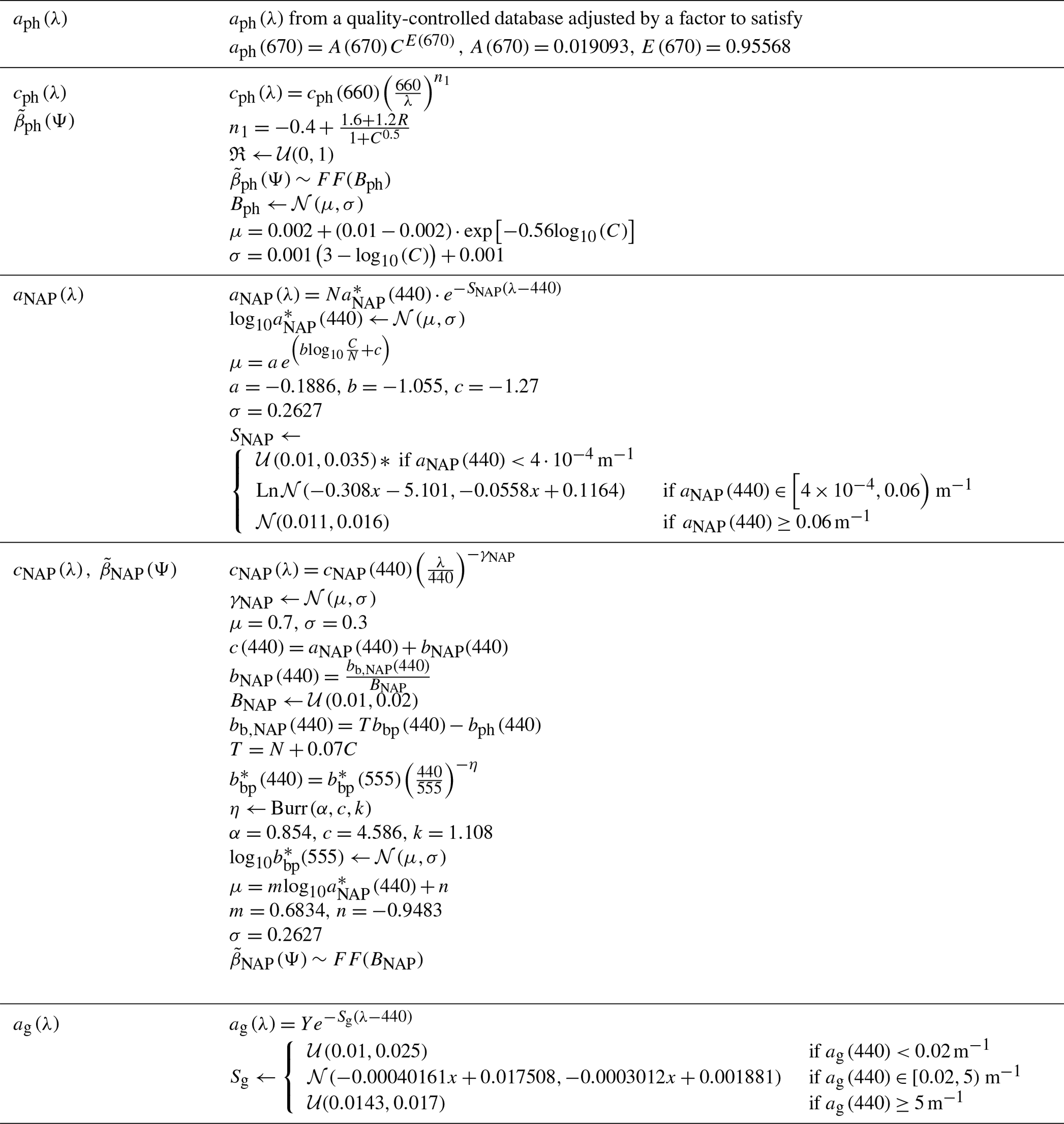
The bio-optical modeling of the various terms of the absorption and scattering budgets as a function of the OACs is explained in high detail in the following sub-sections. Readers interested in a comprehensive summary can find all sequential steps summarized in Table 1.

Table 2 Parameters of the probabilistic modeling of the optically active constituents.

3.1 Optically active constituents

The intention is to generate a SD that covers the widest possible range of optical water types. The historic case 1 assumption is inappropriate, and an IOP definition based on a single index such as chlorophyll concentration (C) is therefore not adopted. Instead, a generic three-variable model is used in which variability is driven by C, N, and Y separately. However, C, N, and Y shall not be completely independent because, if that were the case, the bio-optical modeling would generate unrealistic IOP combinations. Instead, C, N, and Y may be expected to have a certain degree of general relationship, tighter for the smaller values, that are found in the ocean and more scattered for the higher values.

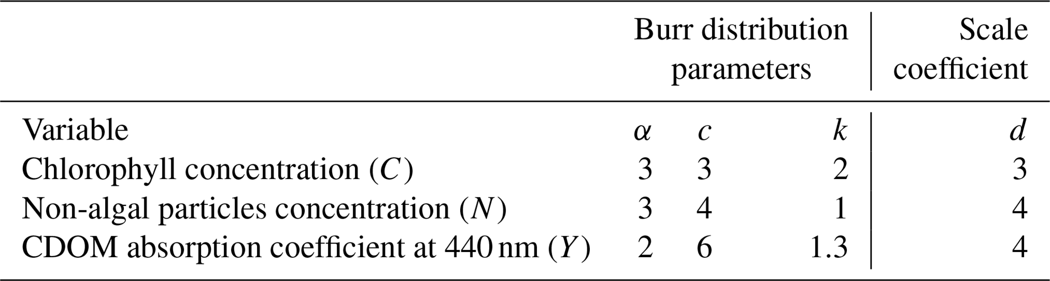
Here, the partial relationship between the three variables on a logarithmic scale was modeled with the generation of 5000 triplets, following three Burr type XII random probability density functions, $\mathit{\alpha }x\leftarrow \mathrm{Burr}(\mathit{\alpha },c,k)$, related by a cross correlation matrix among them with the off-diagonal elements ρ_CN=0.8, ρ_CY=0.75, and ρ_YN=0.6. Then, the derived random numbers were transformed to the actual (C, N, Y), variables with $X={\mathrm{10}}^{x-d}$, where X is either C, N, or Y and x is their logarithmic counterparts. These parameters are summarized in Table 2. Because the Burr distribution does not have an upper bound, it generated very few outliers, C>1000 mg m⁻³, N>2000 g m⁻³, and Y>100 m⁻¹ (∼0.2 % or less), that were considered excessive. Such realizations were re-generated with a log-normal distribution, with the mean and standard deviation calculated from the rest of the dataset.

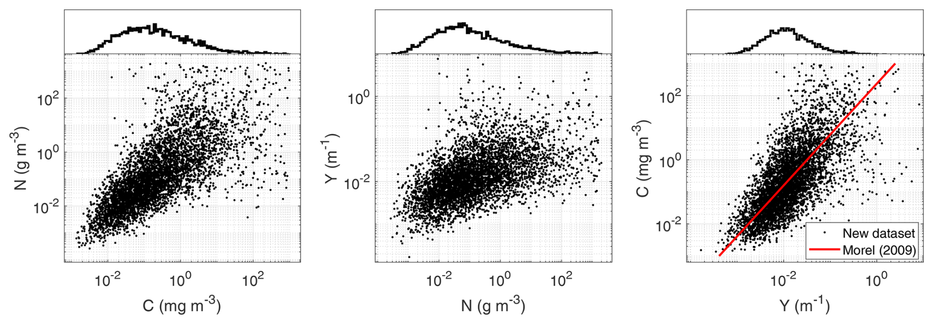
Figure 1 The upper half of each panel shows histograms of the water constituents chlorophyll concentration (C), non-algal particles concentration (N), and CDOM absorption at 440 nm (Y). The lower half of each panel shows the relationships among them. For the relationship between C and Y, the average regression curve by Morel (2009) in oceanic waters is added for comparison.

In Fig. 1, the outcomes of OAC generation are depicted, showcasing broad ranges. The data distributions are skewed, mirroring histograms observed in broad-range datasets: frequencies of data surge from the lower values, peak at levels commonly encountered in global oceans, and gradually taper off at higher extremes. Some degree of an interrelationship is observable, which, in the case of C and Y, shows general agreement with the empirical case 1 curve by Morel (2009). As values ascend, the connection diminishes, which is consistent with expectations for coastal waters.

3.2 Phytoplankton absorption and scattering

Phytoplankton absorption, a_ph, was modeled using data from the pool described in Sect. 2.1. In order to generate phytoplankton diversity, it was important to ensure that, each time, a real a_ph spectrum was used. A similar approach to a_ph generation in the IOCCG SD was followed, but, first, it was found appropriate to revisit the relationship between C and a_ph. Matched data (Valente et al., 2022; Castagna et al., 2022) at several wavelengths (Fig. 2) revealed a tight linear relationship on a log–log scale, though with some scatter, a part of which is attributable due to pigment variation. Following Bricaud et al. (1995), a power-law model (Eq. 8) was regressed at each wavelength:

$$\begin{array}{}\text{(8)}& a_{\mathrm{ph}}\left(\mathit{\lambda }\right)\approx A\left(\mathit{\lambda }\right)C^{E\left(\mathit{\lambda }\right)}.\end{array}$$

Table 3 Output variables and statistical metrics of the regression between matched chlorophyll concentration and phytoplankton absorption of the merged datasets of Valente et al. (2022) and Castagna et al. (2022) at several bands.

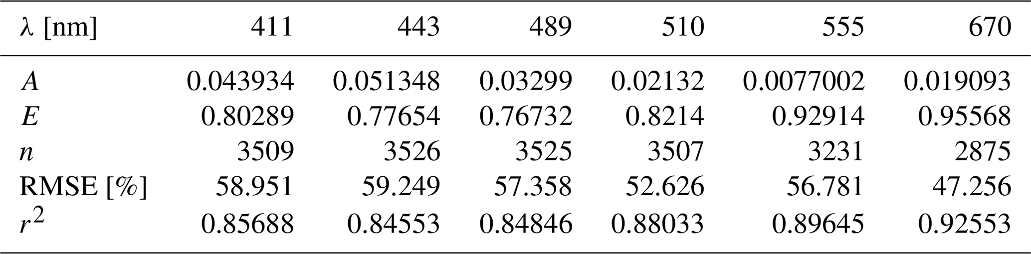
Table 3 presents the regression outcomes, including the two model parameters (A, E), data number (n), root mean square in percent units, and coefficient of determination (r²). A comparison to results from previous publications (Churilova et al., 2023; Bricaud et al., 1995; Zibordi and Berthon, 2024) is made in Fig. 3, showing some discrepancies with respect to the first three references but a high agreement with recent results by Zibordi and Berthon (2024).

Our results show that the 670 nm band has the highest capability for predicting C given a_ph. It is important to emphasize that our modeling does not generate a_ph for a specific C; rather, it associates each a_ph with its characteristic C from the inversion of Eq. (8). This enables us to sort the 3025 a_ph spectra based on C, dividing them into 55 pools of specific C sub-ranges, each containing 55 spectra. Consequently, for a given C value from the (C, N, Y) triplet, a random a_ph spectrum from the corresponding pool is selected. Subsequently, the spectrum is adjusted by a factor so that a_ph(670) equals the predicted a_ph(670) from C after Eq. (8). This methodology guarantees consistency between a_ph and empirical evidence for a given C while ensuring a broad diversity in a_ph spectral shapes.

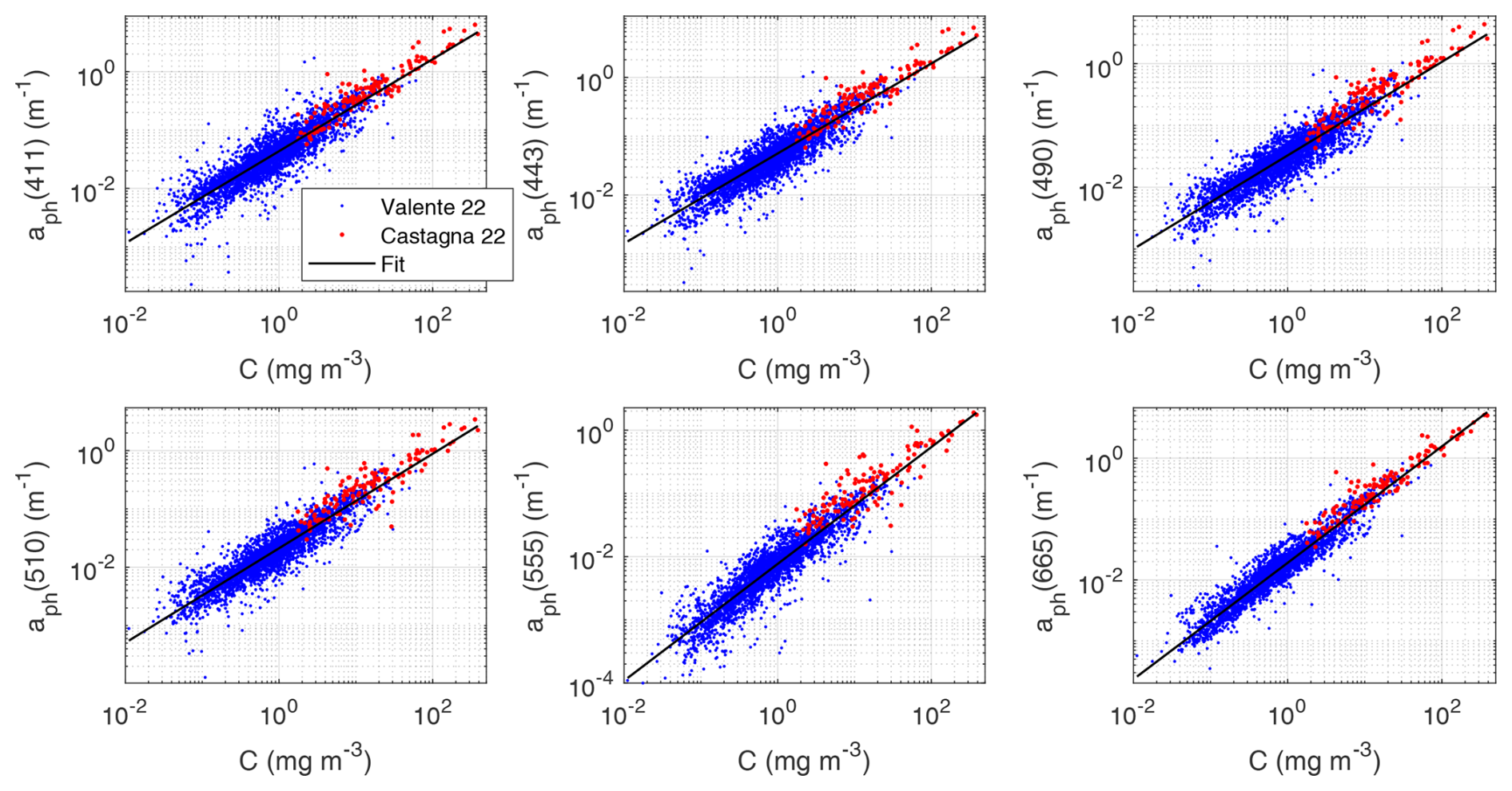
Figure 2 Matched C and a_ph data (Valente et al., 2022; Castagna et al., 2022) at six wavelengths. A linear fit in log–log form is displayed on top.

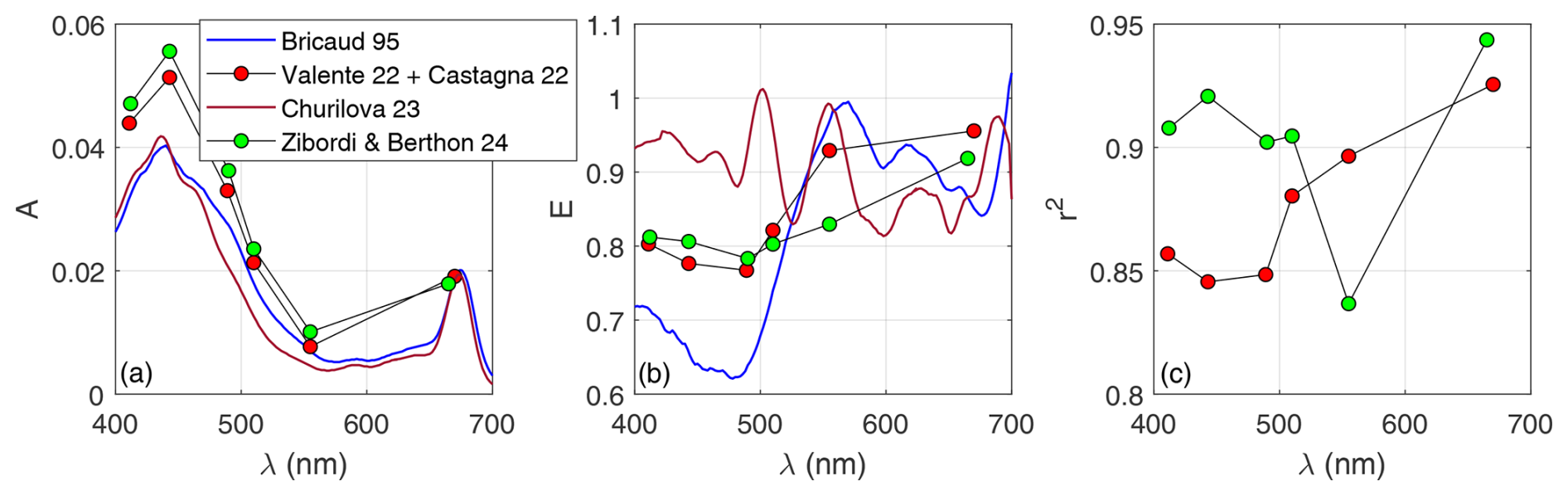
Figure 3 Regression statistics of the fit between C and a_ph data of Fig. 2. Left and center plots are Bricaud's A and E parameters, whereas the right plot is the coefficient of determination (r²).

Phytoplankton scattering (b_ph) modeling is unfortunately based on much less background knowledge, mostly due to the lack of instruments that can measure in situ b_ph or b_b,ph. Electromagnetic modeling of light scattering by particles suspended in water can be applied, although the contributions, albeit notable, are limited (Lain et al., 2023; Poulin et al., 2018). Upon this lack of information, it is often referred to historic measurements by Loisel and Morel (1998) of non-water beam attenuation coefficient at 660 nm c_nw(660) with a transmissometer, matched to chlorophyll concentration in case 1 waters. For surface waters, they found c_nw(660)=0.407C^0.795. Furthermore, the authors reasonably assumed that the dissolved contribution was secondary, so c_p(660)≈c_nw(660). Unfortunately, this relationship was directly exported to phytoplankton scattering modeling used in the CoastColour SD (Nechad et al., 2015), replacing c_p(660) with c_ph(660) and ignoring that even in open sea waters, the non-algal scattering is considerable.

Here, the same generic power-law dependence as in the IOCCG SD (IOCCG, 2006) is used:

$$\begin{array}{}\text{(9)}& c_{\mathrm{ph}}\left(\mathrm{660}\right)=p_{\mathrm{3}}{C}^h.\end{array}$$

According to the IOCCG report, h=0.57, although application of Eq. (9) to the downloadable SD reveals h=0.63. In the CoastColour SD, h=0.795. Here, h=0.7 is used as a balance of both.

p₃ was set to a random value between 0.06 and 0.6 in the IOCCG SD. Interestingly, that leaves the contribution of phytoplankton mostly below what was found by Loisel and Morel (1998) for the total attenuation, which appears physically meaningful. The type of randomness of p₃ was not disclosed, but an inspection to the IOCCG SD revealed that it was uniform. This parameter is modeled here like in the IOCCG SD given the absence of empirical evidence that justifies otherwise.

The spectral variation is set by assigning a power law to c_ph. A power-law function provides a better fit for c_ph than for b_ph as the latter is affected by anomalous dispersion effects that result in some negative peaks with the shape of an a_ph spectrum, which is more evident at high phytoplankton concentrations (Bernard et al., 2009). Interestingly, if the power-law function is imposed on c_ph, the anomalous dispersion feature, b_ph, automatically appears after $b_{\mathrm{ph}}=c_{\mathrm{ph}}-a_{\mathrm{ph}}$. Therefore, in the current SD, neither b_ph nor b_b,ph follow power-law functions.

Regarding the actual exponent of the spectral power law, the same relationship as in the IOCCG SD is used (Eq. 10):

$$\begin{array}{}\text{(10)}& \begin{array}{rl}& c_{\mathrm{ph}}\left(\mathit{\lambda }\right)=c_{\mathrm{ph}}\left(\mathrm{660}\right){\left({\displaystyle \frac{\mathrm{660}}{\mathit{\lambda }}}\right)}^{n_{\mathrm{1}}},\\ & n_{\mathrm{1}}=-\mathrm{0.4}+{\displaystyle \frac{\mathrm{1.6}+\mathrm{1.2}R}{\mathrm{1}+C^{\mathrm{0.5}}}},\end{array}\end{array}$$

with R being a random number that follows a uniform distribution in the interval [0,1].

Given the randomness of a_ph and c_ph, it is possible that some realizations generate cases where a_ph≥c_ph, which is unphysical. A given a_ph represents an assemblage of several phytoplankton communities, each with their specific scattering characteristics, that could be somewhat predicted given a_ph. This information could be extracted from the fine spectral features of a_ph. There are some simplified modeling results using electromagnetic theory for certain phytoplankton species (Lain et al., 2023), although a general modeling theory of phytoplankton scattering linked to absorption is still non-existent. Thus, in this SD, as in the preceding ones (IOCCG, 2006; Nechad et al., 2015; Loisel and Morel, 1998), a_ph and c_ph are modeled independently yet related to the same chlorophyll concentration. To ensure a minimum degree of physical consistency, the procedure for determining a_ph and c_ph was repeated until ensuring a_ph<c_ph at all wavelengths.

The remaining parameter to be set to run HydroLight is the phytoplankton backscattering ratio, $B_{\mathrm{ph}}=\frac{b_{\mathrm{b},\mathrm{ph}}}{b_{\mathrm{ph}}}$. This parameter has not been given much attention in previous research as it was considered relatively unimportant, so it is common to find it set to a constant value on the order of 0.006 or 0.01. It is indeed secondary in semi-analytical algorithms that model R_rs from $\frac{b_{\mathrm{b}}}{a+b_{\mathrm{b}}}$ or variations, but in bio-optical modeling, it can be very relevant if b_ph is fixed first because b_b,ph is then implicitly determined through the choice of the respective phase function given B_ph (Mobley et al., 2002), thereby strongly influencing the intensity of R_rs. Fixing b_b,ph first as a function of C would be another modeling option, for instance, by adapting relationships between b_bp and C found in the ocean (Brewin et al., 2012) to b_b,ph.

In an effort to provide a more accurate determination of B_ph than in previous approaches, we propose a formula that is consistent with the general trend that phytoplankton size increases with C. In its turn, the size increase lowers B_ph because larger particles scatter relatively more in the forward hemisphere with respect to smaller ones, hence lowering B_ph. Twardowski et al. (2001; Fig. 11) presented pioneering results for B_p in their case. Here, to mimic such an effect, it is set to

$$\begin{array}{}\text{(11)}& \begin{array}{rl}& B_{\mathrm{ph}}\sim N\left(\mathit{\mu },\mathit{\sigma }\right),\\ & \mathit{\mu }=\mathrm{0.002}+\left(\mathrm{0.01}-\mathrm{0.002}\right)\exp [-\mathrm{0.56}{\log }_{\mathrm{10}}\left(C\right)],\\ & \mathit{\sigma }=\mathrm{0.001}\left(\mathrm{3}-{\log }_{\mathrm{10}}\left(C\right)\right)+\mathrm{0.001}.\end{array}\end{array}$$

To avoid unlikely low B_ph values after Eq. (11), any realization delivering B_ph<0.001 was set to 0.001 as a lower limit.

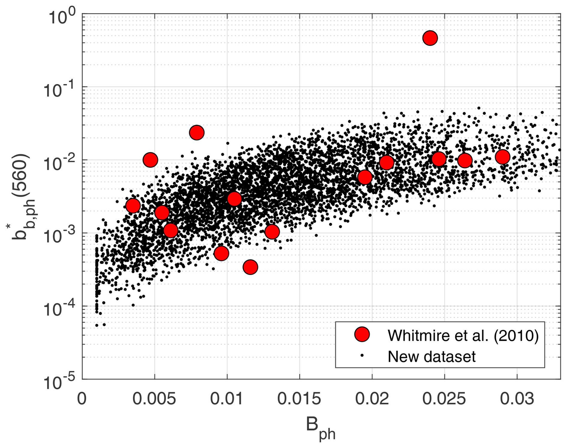
Figure 4 Phytoplankton backscattering ratio, B_ph, vs. phytoplankton specific backscattering coefficient at 560 nm, $b_{\mathrm{b},\mathrm{ph}}^{\ast }\left(\mathrm{560}\right)$. Black dots represent new SD. Red dots represent data in Whitmire et al. (2010).

Independent validation of the modeling of phytoplankton scattering in Eq. (11) is possible, with unique data of chlorophyll concentration matched to scattering and backscattering for an array of phytoplankton cultures by Whitmire et al. (2010). Calculating the chlorophyll-specific phytoplankton backscattering coefficient, i.e., $b_{\mathrm{b},\mathrm{ph}}^{\ast }=\frac{b_{\mathrm{b},\mathrm{ph}}}{C}$ at 560 nm, and matching it to B_ph produces dot clouds in Fig. 4. Our new SD follows the average trend displayed by the Whitmire et al. (2010) in situ data fairly well. Figure 4 also shows some degree of positive covariation between $b_{\mathrm{b},\mathrm{ph}}^{\ast }$ and B_ph. Indeed, $b_{\mathrm{b},\mathrm{ph}}^{\ast }$ decreases with increasing C as well because larger particles have a smaller surface area per unit volume, which diminishes specific scattering. A mechanistic model for b_bp that agrees with this principle was presented in Brewin et al. (2012). All in all, this leads to the visible correlation between B_ph and $b_{\mathrm{b},\mathrm{ph}}^{\ast }$, with the scatter caused by species differences.

3.3 NAP absorption and scattering

Bio-optical modeling of NAP absorption, a_NAP, is complex, as NAP is formed by particles of very diverse nature of biogenic and non-biogenic origin. Modeling approaches (Bengil et al., 2016) are valid as long as the derived relationships hold for the specific area of application. Here, it is aimed at a modeling approach of general validity, consistent with the in situ datasets that were collected from worldwide waters.

Modeling begins with linking a_NAP to the NAP concentration, N, through the specific absorption (to NAP concentration), $a_{\mathrm{NAP}}^{\ast }$. Taking 440 nm as the reference band, other approaches have set it to a constant value (Nechad et al., 2015), although a variability between 0.001 and 0.1 m² g⁻¹ was reported by Blondeau-Patissier et al. (2009). When looking for a predictive formula, one may think that the actual value depends on the type of particles. Following this consideration, the ratio $C/N$ is proposed here as a first-order predictor of $a_{\mathrm{NAP}}^{\ast }\left(\mathrm{440}\right)$. This dependence assumes that NAP absorbs more efficiently in the relatively higher presence of chlorophyll, which suggests that NAP may be of biogenic origin to a larger extent than if the chlorophyll concentration was relatively lower, where NAP may be more of a mineral origin instead. CSIRO data confirmed some degree of covariation (Fig. 5). The fit to the CSIRO data was made on a logarithmic scale, so $y={\log }_{\mathrm{10}}\left[a_{\mathrm{NAP}}^{\ast }\left(\mathrm{440}\right)\right]$ was regressed as a function of $x={\log }_{\mathrm{10}}\left(\frac{C}{N}\right)$, proposing a functional form of the type $y=a\exp \left(bx\right)+c$. A robust regression (bi-square weighting) gave $a=-\mathrm{0.1886}$, $b=-\mathrm{1.0551}$, and $c=-\mathrm{1.2700}$. The standard deviation of the fit was σ=0.2627. To generate the synthetic data, given $C/N$, the regression curve was applied and then a random value, generated with a normal distribution 𝒩(0,σ) was added, in order to replicate the spread found in real data. $\frac{C}{N}$ in our SD covers a wider range than CSIRO's data, so, to avoid producing resulting synthetic $a_{\mathrm{NAP}}^{\ast }\left(\mathrm{440}\right)$ values significantly out of the range of the measured data, the lower and upper bounds of −3 and −0.5 were set for ${\log }_{\mathrm{10}}\left[a_{\mathrm{NAP}}^{\ast }\left(\mathrm{440}\right)\right]$. The results are shown in Fig. 5.

Figure 5 Non-algal particles specific absorption coefficient at 440 nm $a_{\mathrm{NAP}}^{\ast }\left(\mathrm{440}\right)$, plotted as a function of the chlorophyll-to-NAP concentration ratio, $C/N$. Results for CSIRO data are given in red dots, a best fit in blue, and generated data for the SD (black dots).

Posteriorly, it is necessary to project $a_{\mathrm{NAP}}^{\ast }\left(\mathrm{440}\right)$ onto all bands. It can be done by assuming an exponential spectral shape and then guessing the spectral slope (S_NAP). Historic data showed a distribution of S_NAP with an average value of 0.0123 nm⁻¹ (Babin et al., 2003), though with a significant spread. Using a single average S_NAP for all simulations removes optical diversity and likely generates $a_{\mathrm{NAP}}^{\ast }$ spectra that are unlikely for some regions. It is a better choice to generate a prediction function for S_NAP given the available information. After the exponential fits for each of the compiled a_NAP spectra, detailed in Sect. 2.3, the 1349 (a_NAP(λ₀), S_NAP) pairs were plotted together in Fig. 6.

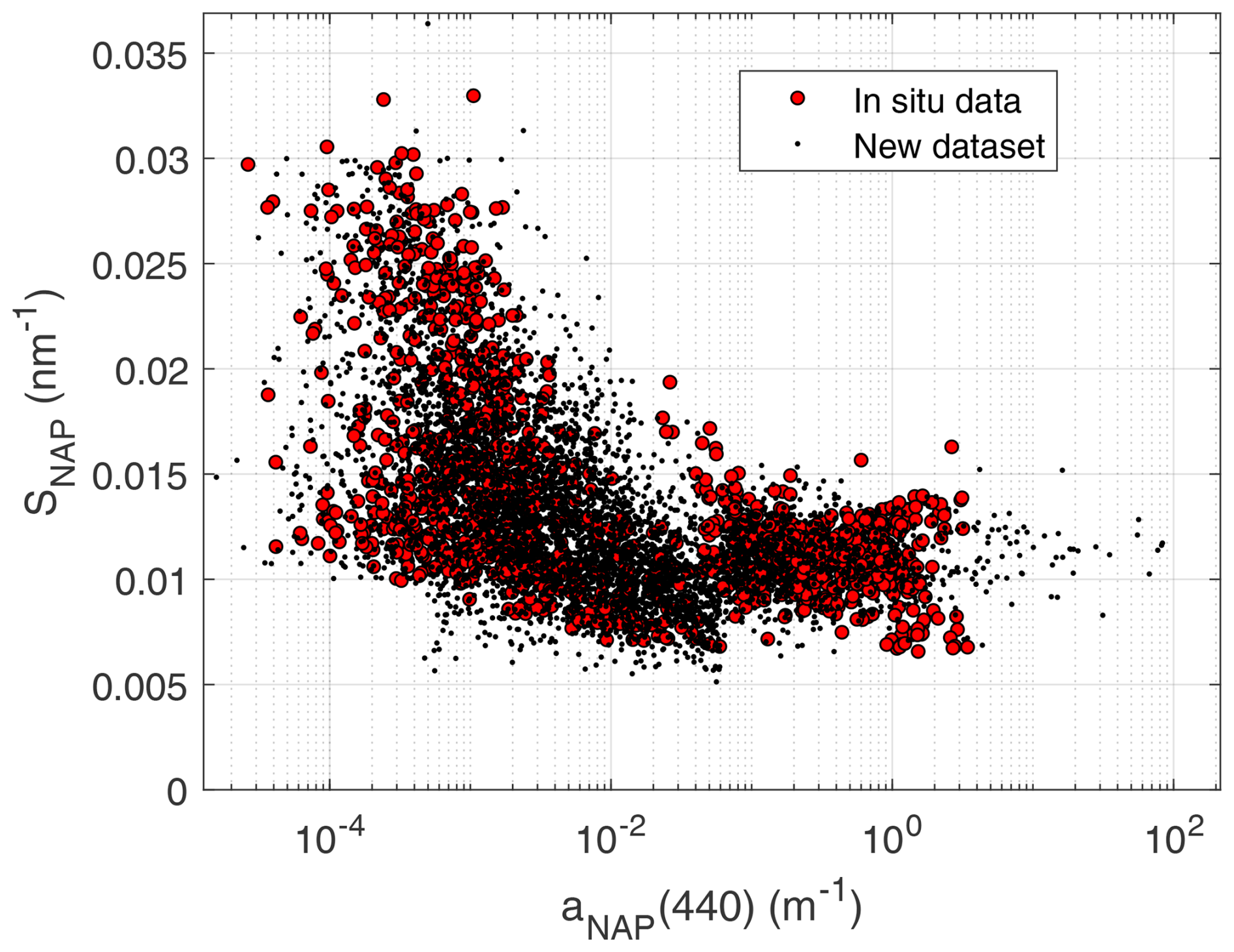
Figure 6 Non-algal particles absorption spectral slope (S_NAP), plotted as a function of the NAP absorption coefficient at 440 nm (a_NAP(440)). Red dots: in situ data. Black dots: synthetic data.

The data distribution in Fig. 6 shows a S_NAP spread that largely varies depending on the a_NAP range. For a very small a_NAP, S_NAP shows no particular pattern between two bounds, so a uniform distribution was found adequate. For the middle range, the S_NAP distribution somewhat narrows as a_NAP(440) increases, and data show some positive skewness, which is well represented by a log-normal curve. For the higher a_NAP(440) range, a Gaussian distribution is apparent, in agreement with Babin et al. (2003). Therefore, given x=log₁₀[a_NAP(440)], S_NAP was modeled as a piece-wise random distribution:

$$\begin{array}{}\text{(12)}& S_{\mathrm{NAP}}\leftarrow \left\{\begin{array}{l}\mathcal{U}\left(\mathrm{0.01},\mathrm{0.035}\right)\text{ if }{a}_{\mathrm{NAP}}\left(\mathrm{440}\right)<\mathrm{4}\times {\mathrm{10}}^{-\mathrm{4}}{\mathrm{m}}^{-\mathrm{1}},\\ \mathrm{Ln}\mathcal{N}\left(-\mathrm{0.308}x-\mathrm{5.101},-\mathrm{0.0558}x+\mathrm{0.1164}\right)\\ \text{if }{a}_{\mathrm{NAP}}\left(\mathrm{440}\right)\in \left[\mathrm{4}\times {\mathrm{10}}^{-\mathrm{4}},\mathrm{0.06}\right){\mathrm{m}}^{-\mathrm{1}},\\ \mathcal{N}(\mathrm{0.011},\mathrm{0.016})\text{ if }{a}_{\mathrm{NAP}}\left(\mathrm{440}\right)\ge \mathrm{0.06}{\mathrm{m}}^{-\mathrm{1}},\end{array}\right.\end{array}$$

where 𝒰(a,b), Ln𝒩(μ,σ), and 𝒩(μ,σ) are the uniform, log-normal, and normal distributions, respectively. The random parameterization for S_NAP in Eq. (12) is rather convoluted. However, it ensures fitness to a high quality and large in situ dataset, and it does not generate outliers, as can be seen when overlapping the synthetic data to the field data in Fig. 6.

NAP scattering needs bio-optical modeling too. Approaches that model NAP absorption and scattering independently may generate unrealistic IOPs for that particular material. It is beneficial to look for relationships that link NAP scattering to NAP absorption as it is expected to occur in natural waters. The CSIRO dataset contains $b_{\mathrm{bp}}^{\ast }\left(\mathrm{555}\right)$ data, concurrent with $a_{\mathrm{NAP}}^{\ast }\left(\mathrm{440}\right)$. It must be clarified that, while $a_{\mathrm{NAP}}^{\ast }\left(\mathrm{440}\right)$ is specific of N, $b_{\mathrm{bp}}^{\ast }$ has been defined by normalizing b_bp to the total suspended matter concentration (T), which is not to be confused with non-algal particles concentration N, as the latter is only a fraction of the former, which also contains the phytoplanktonic part. Brando and Dekker (2003) proposed a somewhat crude relationship, $T=N+\mathrm{0.07}C$, where both T and N are expressed in the usual units of g m⁻³ and C is in mg m⁻³. For interested readers, such a relationship was derived from measurements in a shallow, turbid, and eutrophic lake in the Netherlands (Gons et al., 1992).

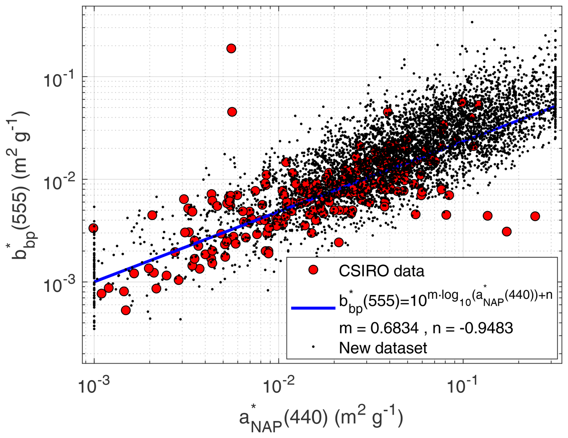
Figure 7 Specific particle backscattering coefficient at 555 nm $b_{\mathrm{bp}}^{\ast }\left(\mathrm{555}\right)$, plotted as a function of the non-algal particles specific absorption coefficient at 440 nm $a_{\mathrm{NAP}}^{\ast }\left(\mathrm{440}\right)$. Results for CSIRO data in red dots, the best linear fit in blue, and generated data for the SD (black dots).

The relationship between $a_{\mathrm{NAP}}^{\ast }\left(\mathrm{440}\right)$ and $b_{\mathrm{bp}}^{\ast }\left(\mathrm{555}\right)$ data is very marked (Fig. 7, red dots). A linear trend was a very good fit between the log-transformed variables, with a slope m=0.6834 and an intercept $n=-\mathrm{0.9483}$. The data spread followed a normal distribution (σ=0.2627) after removing the trend line. To reproduce this spread in the SD, a random number following a random normal distribution N(0,σ) was added to the fit-predicted $b_{\mathrm{bp}}^{\ast }\left(\mathrm{555}\right)$ prior to the conversion to linear scale again. Results of the data cloud generated are seen in Fig. 7 (black dots).

Completing the bio-optical modeling for NAP requires the projection of $b_{\mathrm{bp}}^{\ast }$ from 555 to 440 nm. CSIRO data provide an estimate of the particle backscattering spectral slope (η) for every data point. For synthetic data generation, a modeling function for η must be derived. No relationship between η and any other parameter within the CSIRO dataset was found. Its histogram was fitted well, with a random Burr distribution and the parameters α=0.854, c=4.586, and k=1.108, shown in Fig. 8. Therefore, η was randomly generated using this distribution.

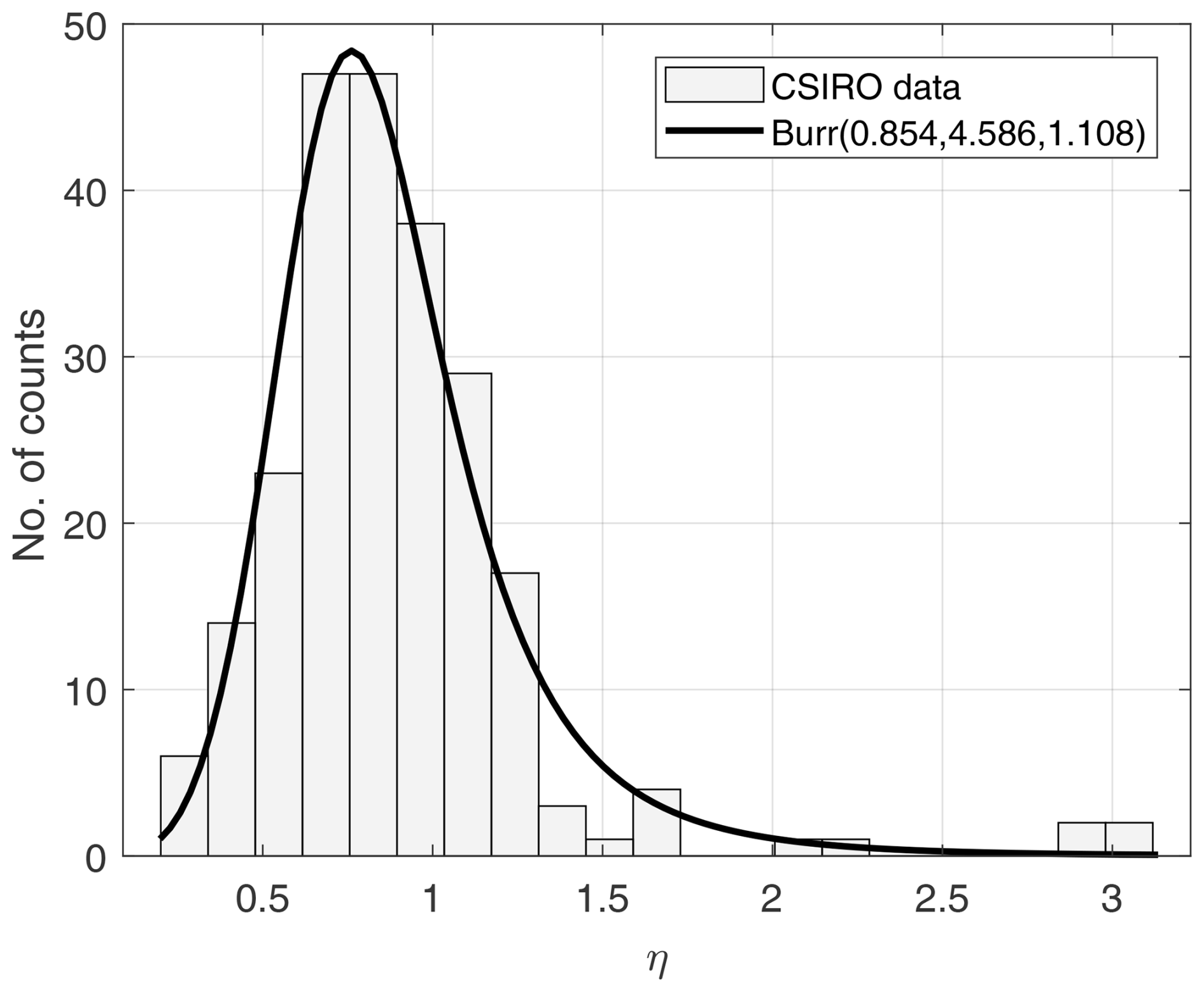
Figure 8 Histogram of the particle backscattering coefficient spectral slope (η). A Burr type XII fitted distribution is plotted on top.

With η determined, $b_{\mathrm{bp}}^{\ast }$ was shifted to 440 nm: $b_{\mathrm{bp}}^{\ast }\left(\mathrm{440}\right)=b_{\mathrm{bp}}^{\ast }\left(\mathrm{555}\right){\left(\frac{\mathrm{440}}{\mathrm{555}}\right)}^{-\mathit{\eta }}$. It must be remarked that this b_bp slope is only used in this step and that it is not used to model b_bp with a power law in the SD. In the bio-optical modeling of NAP and of phytoplankton, a spectral shape is assumed for attenuation and not for backscattering.

The NAP backscattering at 440 nm was derived in Eq. (13) by the subtraction of the phytoplanktonic part, which is known from Sect. 3.2:

$$\begin{array}{}\text{(13)}& b_{\mathrm{b},\mathrm{NAP}}\left(\mathrm{440}\right)=b_{\mathrm{bp}}^{\ast }\left(\mathrm{440}\right)\cdot T-b_{\mathrm{b},\mathrm{ph}}\left(\mathrm{440}\right).\end{array}$$

A backscattering ratio for NAP (B_NAP) must be assumed to obtain b_NAP(440) and c_NAP(440). There are no direct measurements of B_NAP given the current impossibility of measuring NAP scattering parameters in the field. Nevertheless, this poses a minor problem for radiative transfer calculations, especially in remote-sensing applications. As long as b_b,NAP is fixed, B_NAP is relatively unimportant as one can deduct from simplified analytical models for reflectance or diffuse attenuation. If b_NAP was fixed instead, B_NAP would be a fundamental parameter as it would implicitly set b_b,NAP in a much less accurate fashion. B_NAP was fixed as a random number here, following a uniform distribution between 0.01 and 0.02 as in Eq. (15):

$$\begin{array}{}\text{(14)}& B_{\mathrm{NAP}}\leftarrow \mathcal{U}\left(\mathrm{0.01},\mathrm{0.02}\right).\end{array}$$

Then, the scattering coefficient of NAP was determined with Eq. (15):

$$\begin{array}{}\text{(15)}& b_{\mathrm{NAP}}\left(\mathrm{440}\right)={\displaystyle \frac{b_{\mathrm{b},\mathrm{NAP}}\left(\mathrm{440}\right)}{B_{\mathrm{NAP}}}}.\end{array}$$

Then, the NAP attenuation at 440 nm was expressed in Eq. (16) as a function of values that are all known:

$$\begin{array}{}\text{(16)}& c_{\mathrm{NAP}}\left(\mathrm{440}\right)=a_{\mathrm{NAP}}^{\ast }\left(\mathrm{440}\right)\cdot N+b_{\mathrm{NAP}}\left(\mathrm{440}\right).\end{array}$$

The remaining step for NAP modeling is extending NAP attenuation to all wavelengths. As for phytoplankton, a power law is assumed, and it is preferred to impose it on attenuation than scattering, though recognizing that, given the much featureless shapes of NAP absorption, a fit to scattering may be realistic too. A c_NAP spectral slope, γ_NAP, must be assumed. This parameter is largely unknown as it cannot be measured in the field. Here, an educated guess is made, generating γ_NAP randomly, with ${\mathit{\gamma }}_{\mathrm{NAP}}\leftarrow \mathcal{N}(\mathrm{0.7},\mathrm{0.3})$. Therefore, Eq. (17) completes the NAP modeling:

$$\begin{array}{}\text{(17)}& c_{\mathrm{NAP}}\left(\mathit{\lambda }\right)=c_{\mathrm{NAP}}\left(\mathrm{440}\right){\left({\displaystyle \frac{\mathrm{440}}{\mathit{\lambda }}}\right)}^{{\mathit{\gamma }}_{\mathrm{NAP}}}.\end{array}$$

3.4 CDOM absorption

The 1168 (a_g(λ₀), S_g) pairs, calculated in Sect. 2.2 are plotted together in Fig. 9. The middle section shows a data spread whose mean and standard deviation decrease with a_g(440). Variation in the lower and upper range ends could not be linked to any parameter, so S_g was modeled as uniform distributions fairly within the data range. Overall, S_g was then modeled as a piece-wise random distribution given x=log₁₀[a_g(440)].

$$\begin{array}{}\text{(18)}& S_{\mathrm{g}}\leftarrow \left\{\begin{array}{l}\mathcal{U}\left(\mathrm{0.01},\mathrm{0.025}\right)\text{ if }{a}_{\mathrm{g}}\left(\mathrm{440}\right)<\mathrm{0.02}{\mathrm{m}}^{-\mathrm{1}}\\ \mathcal{N}\left(-\mathrm{0.00040161}x+\mathrm{0.017508},-\mathrm{0.0003012}x\right.\\ \left.+\mathrm{0.001881}\right)\text{ if }{a}_{\mathrm{g}}\left(\mathrm{440}\right)\in \left[\mathrm{0.02},\mathrm{5}\right){\mathrm{m}}^{-\mathrm{1}}\\ \mathcal{U}(\mathrm{0.0143},\mathrm{0.017})\text{ if }{a}_{\mathrm{g}}\left(\mathrm{440}\right)\ge \mathrm{5}{\mathrm{m}}^{-\mathrm{1}}\end{array}\right.\end{array}$$

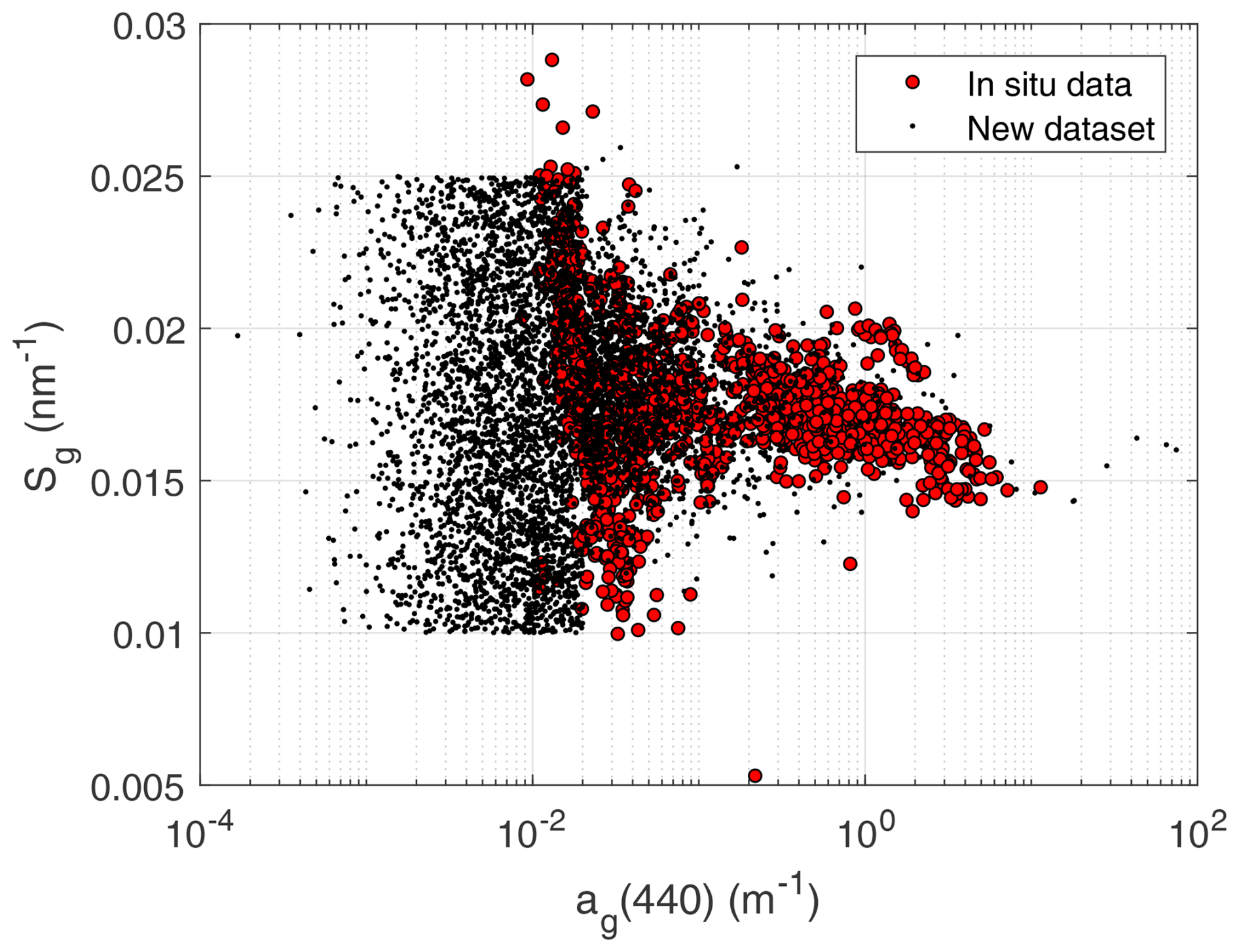
Figure 9 CDOM spectral slope (S_g) plotted as a function of the CDOM absorption coefficient at 440 nm (a_g(440)). Red dots represent in situ data. Black dots represent synthetic data.

Figure 9 compares the field (a_g(λ₀), S_g) pairs to those generated with the combination of random distributions in Eq. (18). It can be seen that the SD includes an order of magnitude more of a_g(440) at the lower end than the in situ data in Fig. 9. This is due to the very stringent condition of exponential variation set in Sect. 2.2 that mostly affected the low a_g spectra. In terms of predicting S_g, extrapolation may raise some concerns, but on the one hand, S_g values are well bounded in this part of the range, and on the other hand, one must also note that a_g(440) becomes very low, so potential errors in S_g are not relevant for the absorption budget. In terms of the data range, it is shown in Sect. 4.1 that the lowest a_g(440) in the SD is on the order of a_g(440) in the most oligotrophic oceans.

3.5 Pure water absorption and scattering

Pure liquid water absorbs electromagnetic radiation, which can be mechanistically explained as the energy consumption by the two O–H molecular bonds needed to vibrate at given resonant frequencies, creating an absorption spectrum, a_w, with characteristic maxima and minima at specific wavelengths. In practice, a_w must be measured at a wide enough spectral range, and its values must be tabulated for usage in bio-optical modeling. However, literature only offers partial spectral-range a_w measurements, owing to the specific requirements and challenges inherent in such measurements. A broad-range a_w must then be a merged product from individual sources. A crucial step here involves compensating for the different temperatures at which a_w was measured in different laboratories and, in the spectral ranges where different measurements are available, selecting those of the highest quality that are retained. Fortunately, this process had already been undertaken within the framework of an ESA project (Roettgers et al., 2016), where the water optical properties processor (WOPP) produced a dataset of pure water absorption, normalized to 20 °C. Notably, this dataset encompasses measurements by Mason et al. (2016) from UV to green wavelengths, revealing lower water absorption in the UV and blue regions than previously documented thanks to meticulous sample preparation and precise measurements. In other spectral regions, data from various authors are merged, sometimes overlapping spectrally and sometimes not. Overall, the WOPP pure water absorption data can be considered the state of the art. For comprehensive insights, readers are directed to the project report.

When marine salts are dissolved in water, the ions dissociate and create a stable solution whose absorption can be related to that of pure water proportionally to the salinity (Ψ_S) dependent on the wavelength. Temperature affects absorption in a similar manner through Ψ_T, thus leading to

$$\begin{array}{}\text{(19)}& a_{\mathrm{w}}\left(T,S\right)=a_{\mathrm{w}}\left(T_{\mathrm{0}},\mathrm{0}\right)+{\mathrm{\Psi }}_{\mathrm{T}}\left(T-T_{\mathrm{0}}\right)+{\mathrm{\Psi }}_{\mathrm{S}}S.\end{array}$$

Both Ψ_T and Ψ_S can be empirically determined. To the WOPP pure water merged absorption, a shift to an average ocean salinity of S=35 PSU was made with Eq. (19) using the Ψ_S coefficient provided by Roettgers et al. (2014) for artificial seawater.

Scattering by pure water finds explanation with the Smoluchowski–Einstein fluctuation theory of light scattering (Zhang and Hu, 2021), according to which a certain volume of water can be seen as consisting of smaller sub-volumes that contain, on average, the same number of water molecules. However, the instantaneous numbers vary among them due to random thermal motions at the molecular level, resulting in microscopic density fluctuations that induce scattering. In the presence of solutes such as salts, this effect is magnified as fluctuations in the spatial arrangement of dissolved ions lead to variations in the overall refractive index. For common ocean salinities, scattering is augmented by approximately 30 % with respect to fresh water. Recent work by Zhang and Hu (2021) provide a comprehensive review of this theory, offering the most precise estimates to date (likely within ±2 %–4 %). Nevertheless, rigorous experimental validation remains imperative. The formulas provided as supplementary material in their paper were employed to compute seawater scattering, assuming a temperature of T=20 °C and a salinity of S=35 PSU, as for the absorption data.

Figure 10 IOP cross-relationship comparison between the SD and various in situ datasets.

Figure 11 IOP cross-relationship comparison between this and other SDs.

4 Results of the synthetic dataset

4.1 Modeled IOPs

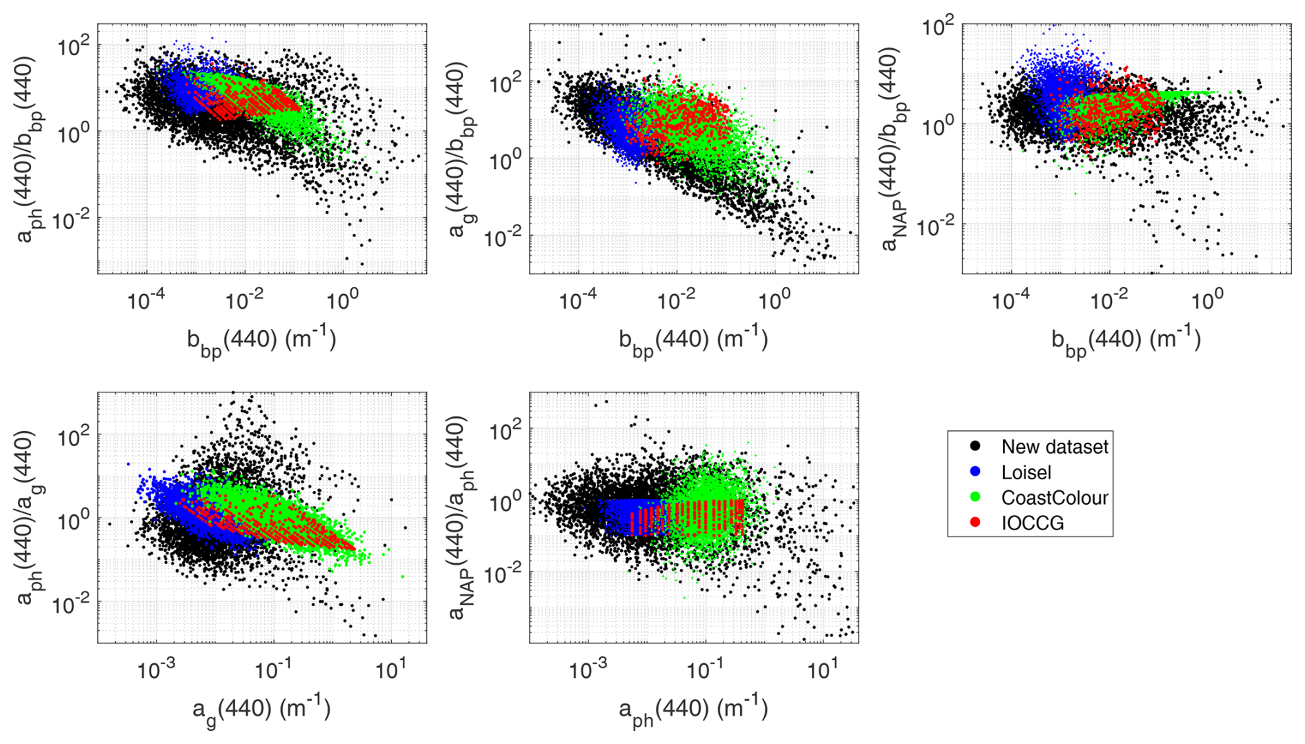
The bio-optical modeling detailed in the Sect. 3 generated the IOPs that determine the resulting light field and related AOPs given the boundary conditions. These bio-optical relationships have been individually assessed, and consistency with literature and with new data is ensured in that section. However, the overall result of the bio-optical modeling can be tested by checking the crossed relationship between different commonly measured IOPs at specific wavelengths, compared to in situ data, in order to verify that the relationships that are found in the world's waters are represented.

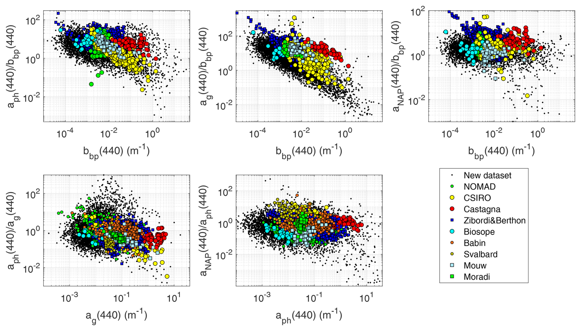
In situ datasets were searched that contained IOP data at the reference wavelength of 440 nm. The following publicly available data were used: the PACE data, including the Biosope cruise data from the clearest ultraoligotrophic waters of the south Pacific gyre, with some stations in coastal upwelling water off Peru and Mouw's data in Lake Superior (Casey et al., 2020); the NOMAD dataset (Werdell and Bailey, 2005); the Castagna et al. (2022) data in Belgian coastal and inland waters; the measurements in coastal European waters (Massicotte et al., 2023); the measurements in Svalbard (Petit et al., 2022) and a recently published dataset in European seas (Zibordi and Berthon, 2024). In addition, two datasets not yet publicly available were queried from the authors, who kindly sent them for use in this article: data from the Persian Gulf (Moradi and Arabi, 2023) and from Australian waters (Blondeau-Patissier et al., 2009, 2017; Cherukuru et al., 2016; Oubelkheir et al., 2023; Brando et al., 2012). The Castagna et al. (2022) data lacked b_bp, but since such a dataset was considered unique and relevant, b_bp was inferred through semi-analytic closure from absorption and R_rs (Lee et al., 2011).

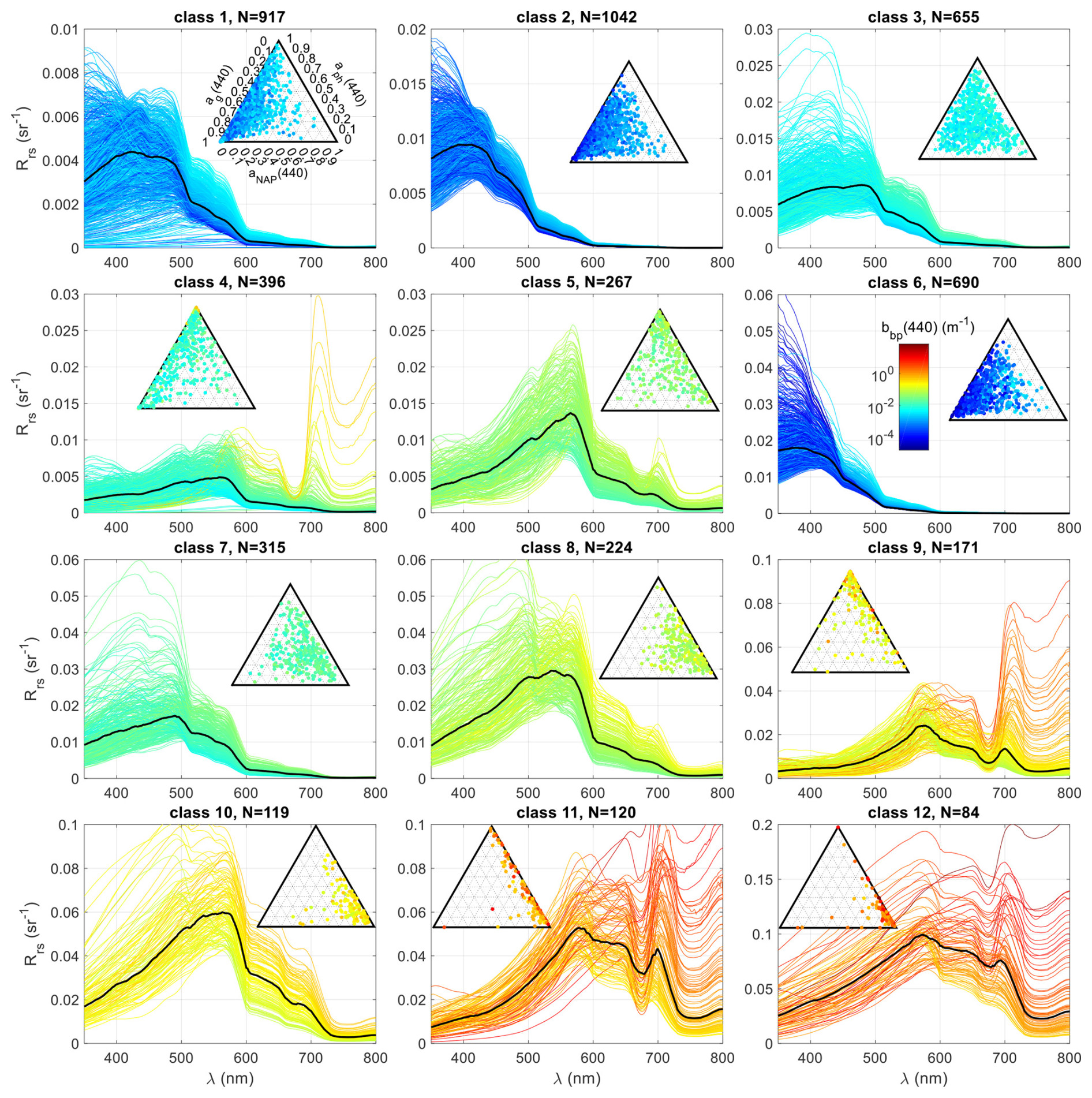
Figure 12 R_rs spectra (normalized geometry) of the SD divided into 12 classes using the k-means classifying algorithm, with their total number (N) indicated above. Relative to each class, the ternary plots of the absorption budget are plotted. The line and dot colors indicate particle backscattering at 440 nm according to the attached color bar. Note the varying vertical scale, across the classes, necessary to visualize the spectral variability across the dynamic ranges.

Figure 10 presents relationships among various IOPs at the reference wavelength of 440 nm. The upper panels study the three non-water absorption components with respect to particle backscattering, and the two lower panels compare the different absorption compartments. Because the two given IOPs are expected to linearly covary to the first degree, the vertical axis plots the ratio between the two so that the linear covariation is eliminated, restricting the dynamic range and highlighting the differences among datasets. The plots show that available measurements in different geographic areas and seasons cover different regions of the data space and that the SD globally encompasses all of them, notably extending the data volume in oligotrophic oceanic waters, which are geographically large but grossly under-sampled. Overall, this figure provides rather robust evidence that the SD has global coverage, from the clearest oceans to all kinds of coastal waters, and that the bio-optical relationships adopted in this study are in line with empirical evidence.

This SD is also compared to the three publicly available SDs in Fig. 11: the IOCCG SD (IOCCG, 2006), the CoastColour SD (Nechad et al., 2015), and the Loisel et al. (2023) SD. Some overlap is noticeable for all crossed IOPs, with the Loisel et al. (2023) SD being shifted more towards clearer waters than IOCCG and CoastColour. Also, this SD shows trends that appear more consistent with our SD. The CoastColour SD covers the upper part of the range, but due to its optical modeling, many dots are clustered near each other instead of covering a wider range of values. The new SD covers a wider range of waters than the other SDs combined, which is a consequence of not only the broad ranges for the OACs, but also the adequate amount of statistical randomness that was given to the bio-optical relationships.

4.2 Radiative transfer calculations

Radiative transfer simulations were made with HydroLight 5.1.2 (Sequoia Scientific, Inc.). Normalized sky radiances were computed using the sky model HCNRAD (Harrison and Coombes Normalized RADiances) (Harrison and Coombes, 1988). Diffuse and direct sky irradiances were computed using the RADTRANX (RADTRAN eXtended for 300–1000 nm) model (Gregg and Carder, 1990). The ozone concentration was estimated from a climatology derived with binned monthly average TOMS v8 ozone concentrations (data from 2000–2004 were averaged to give 5-year climatological averages for 5° latitude and 10° longitude quadrants) for the 90th day of the year, coordinates 40° N and 0° E, resulting in 354.9 DU. The US Navy aerosol model was fed with the values: air mass type 5, relative humidity of 80.0 %, precipitable water of 2.5 cm, and horizontal visibility of 40.0 km. Sea surface roughness was modeled with a HydroLight-embedded Monte Carlo module fed with an assumed wind speed of 5.0 m s⁻¹. The water index of refraction was calculated as a function of wavelength (Roettgers et al., 2016) for the given seawater, T=20.0 °C and S=35.0 PSU. The sea was considered vertically homogeneous and infinitely deep. IOP input was configured with a generic case 2 water scenario. Input IOP parameters and phase functions were set as detailed in Table 1. Inelastic scattering effects were not considered.

The source code of HydroLight was modified so that the “printout” output files included reflectances, both above and below the surface, for the whole set of viewing zenith and azimuth angles defined by HydroLight default quadrants, that is, a view angle varying from 0 to 80° in steps of 10° and then a last value of 87.5° (10 values in total) and the azimuth varying from 0 to 180° in steps of 15° (13 values in total). Simulations were made for the whole range of sun zenith angles defined by the quadrants, that is from 0 to 80° in steps of 10° and then a last value of 87.5° (10 values in total). Therefore, for every IOP setup, directional AOPs are given at 1300 angles, and non-directional AOPs are given at the 10 sun zenith angles.

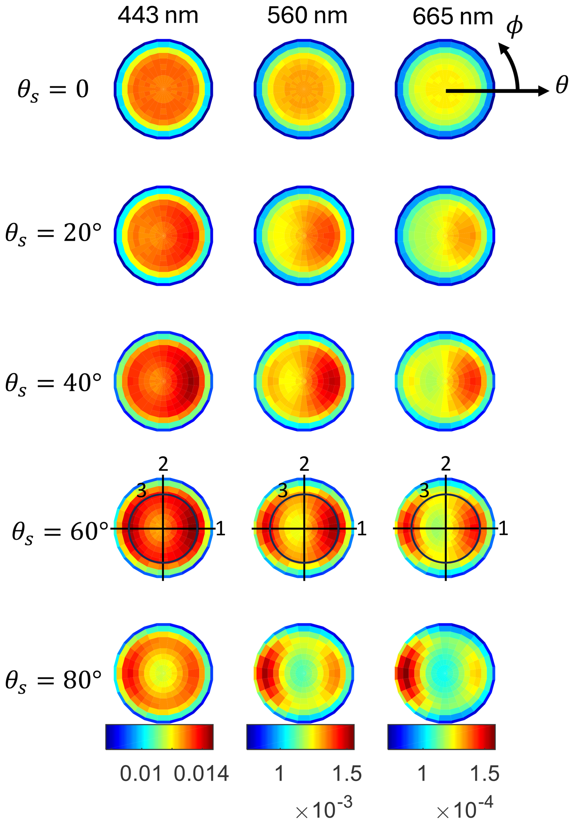
Figure 13 Angular variability in R_rs for the oligotrophic water spectrum shown in Fig. 14. The polar plots are divided into selected sun zenith angles (rows) and wavelengths (columns). The polar angle represents the azimuth (zero “looking at the sun”), while the radius represents the radiance propagation angle (same as the viewing zenith angle). The color represents the R_rs magnitude. The color scale among wavelengths for visualization purposes. For θ_s=60° specifically, some indicated slices are presented in 1D plots in Fig. 14. Section 1: sun's meridian plane. Section 2: perpendicular plane to the sun's meridian plane. Section 3: constant θ=60°.

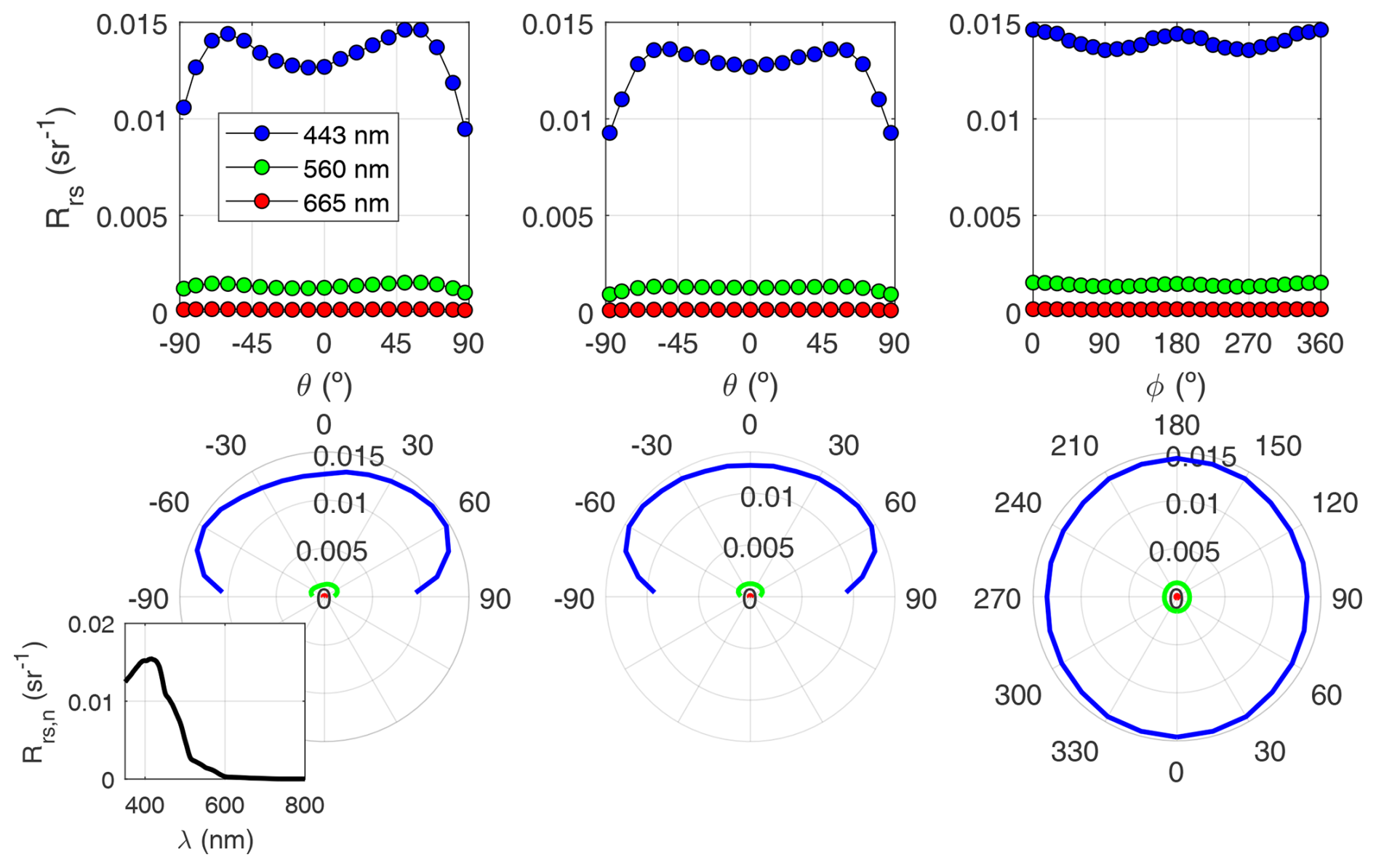
Figure 14 Angular variability in HydroLight-simulated R_rs for the oligotrophic water case (spectrum shown in the corner). The plots represent the three sections for θ_s=60° in Fig. 13 in consecutive columns. Here, the sections are plotted in Cartesian coordinates in the upper plots and polar coordinates in the lower ones.

4.3 Reflectance overview and classification

Synthetic R_rs was scrutinized to ensure that a diverse range of optical water types had been produced. The data underwent partitioning into 12 clusters via a k-means algorithm (Fig. 12). Ternary plots were employed to visualize the absorption budget for all R_rs values within each class, with curves and dots colored based on particle backscattering. This classification is only used here as a method to show the extensive optical diversity within the SD and does not constitute a part of it. Descriptively, the water types are as follows:

• Classes 2 and 6 relate to clear oceanic waters.

• Class 1 corresponds to highly absorbing waters, with little NAP content.

• Classes 3, 5, 7, and 8 represent coastal waters, exhibiting moderate concentrations of all constituents, in varying proportions.

• Classes 4 and 9 display highly productive waters, marked by high CDOM and NAP levels, respectively.

• Classes 10, 11, and 12 portray highly and very highly turbid waters. Notably, despite categorizing this water type into three classes, their cumulative occurrence is discrete. This outcome stems from the classification, which accentuates disparities in R_rs values that are high.

4.4 Angular variation

Besides the wide IOP ranges, a unique characteristic of this SD is the resolution of the AOPs for the whole range of sun-view geometries. This matter is relevant for algorithm development and validation; for instance, in either in situ or satellite R_rs, the sun is very rarely at the zenith. The view angle is off nadir in above-water platforms and in satellite data, and the azimuth is normally such that it avoids maximum sun glint. This R_rs bidirectionality is very often ignored. Algorithms that use band ratios, such as the oceanic OCx, partially suppress the bidirectional effect because its spectral pattern is quite flat, but algorithms that rely on the absolute magnitude of R_rs will inevitably propagate bidirectional effects as errors. This section showcases the anisotropy of R_rs for two distinct water types. The first represents very oligotrophic oceanic waters, while the second relates to more productive waters. The azimuthal angle definition follows that of HydroLight (i.e., solar photons travel in the ϕ=180° direction; that is, the sun is located at ϕ=0).

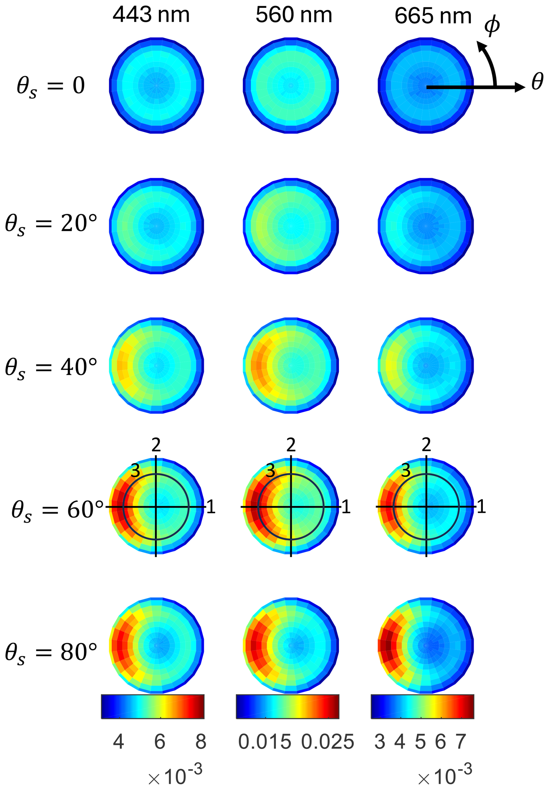
Figure 15 As in Fig. 13 but for the angular variability in R_rs for the productive water case.

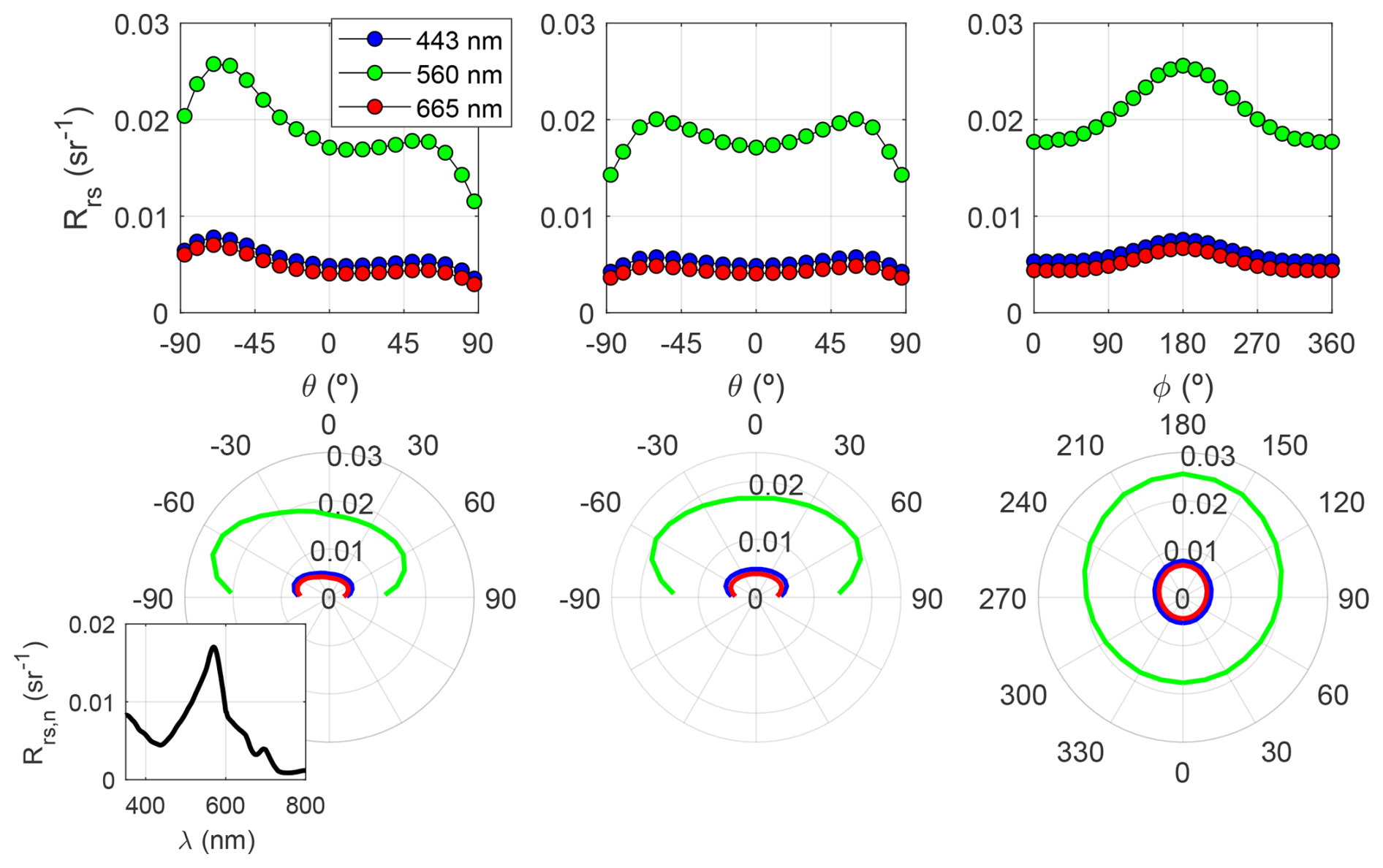
Figure 16 As in Fig. 14 but for the angular variability in R_rs for the productive water case.

A first example of the R_rs anisotropy for a clear water scenario is displayed in Fig. 13 for three wavelengths and five sun zenith angles. The related Fig. 14 focuses on one sun zenith angle (θ_s=60°), the sun's meridian plane ($\mathit{\varphi }=\mathrm{0},\mathrm{180}$°) and its perpendicular vertical plane ($\mathit{\varphi }=-\mathrm{90},\mathrm{90}$°), and a constant zenith view section (θ=60°), all cases for a reference sun zenith angle (θ_s=60°). Increasing the sun zenith lowers the azimuthal symmetry and strengthens the radiance anisotropy. A zone of higher values forms along the solar plane for ϕ=0. It is known that, for very clear waters, the single-scattering approximation can, at least qualitatively, explain the results. The phase functions of both water and particles have a local maximum at a scattering angle of Ψ=180°, leading to an overall maximum at θ=60°, that is, the backscattering direction. The secondary maximum at $\mathit{\theta }=-\mathrm{60}$° (or θ=60° for ϕ=180°) can be explained by the balance between a progressive increase in the particle phase function and a decrease in the water phase function as Ψ decreases.

Figures 15 and 16 show an analog example for a productive water scenario. Notable is the azimuthal maximum shift to the ϕ=180° direction. This is explained by the dominance of the particle phase function and the appearance of multiple scattering, which starts to become important even for small concentrations. This implies that the radiance at an angle of $\mathit{\theta }=-\mathrm{70}$° (or θ=70° for ϕ=180°) is less influenced by the shape of the phase function at the particular direction given by the single scattering direction. Instead, multiple scattering makes the resulting radiances influenced by the phase function in variable ranges reaching Ψ<120°, where it increases sharply. Indeed, multiple scattering does not generate isotropy in R_rs, as might be believed by some, but instead changes the angular pattern of the anisotropy. This behavior, although already documented (Loisel and Morel, 2001), was somehow not assimilated by most within the community.

4.5 Reflectance validation with in situ data

The number of relationships imposed to the IOPs, as well as the cross-checks among them, gives confidence in the realism of the SD generated. Yet to be further confident that the synthetic AOPs represent natural waters, it is desirable to show some comparison to in situ data that involve the AOPs themselves.

We evaluated in Fig. 17 the R_rs (normalized geometry) of our entire SD through the spectral quality index (QWIP) by Dierssen et al. (2022). Such an index aims at providing a quality estimate for a hyperspectral R_rs. QWIP developed a large dataset of in situ R_rs, so this comparison can be seen as a comparison to real R_rs data. In Dierssen et al. (2022), it is mentioned that values within the 0.2 margins have a high similarity to real spectra measured in the field, which, for the case of the SD, is verified in 4993 out of the 5000 spectra. Still, these seven spectra are close to the limit and may simply contain some bio-optical characteristics that were not present in the QWIP calibration dataset. No spectra are clearly off from the main trend line, thus giving confidence in the quality of our SD in terms of this index and of the data from which it was derived.

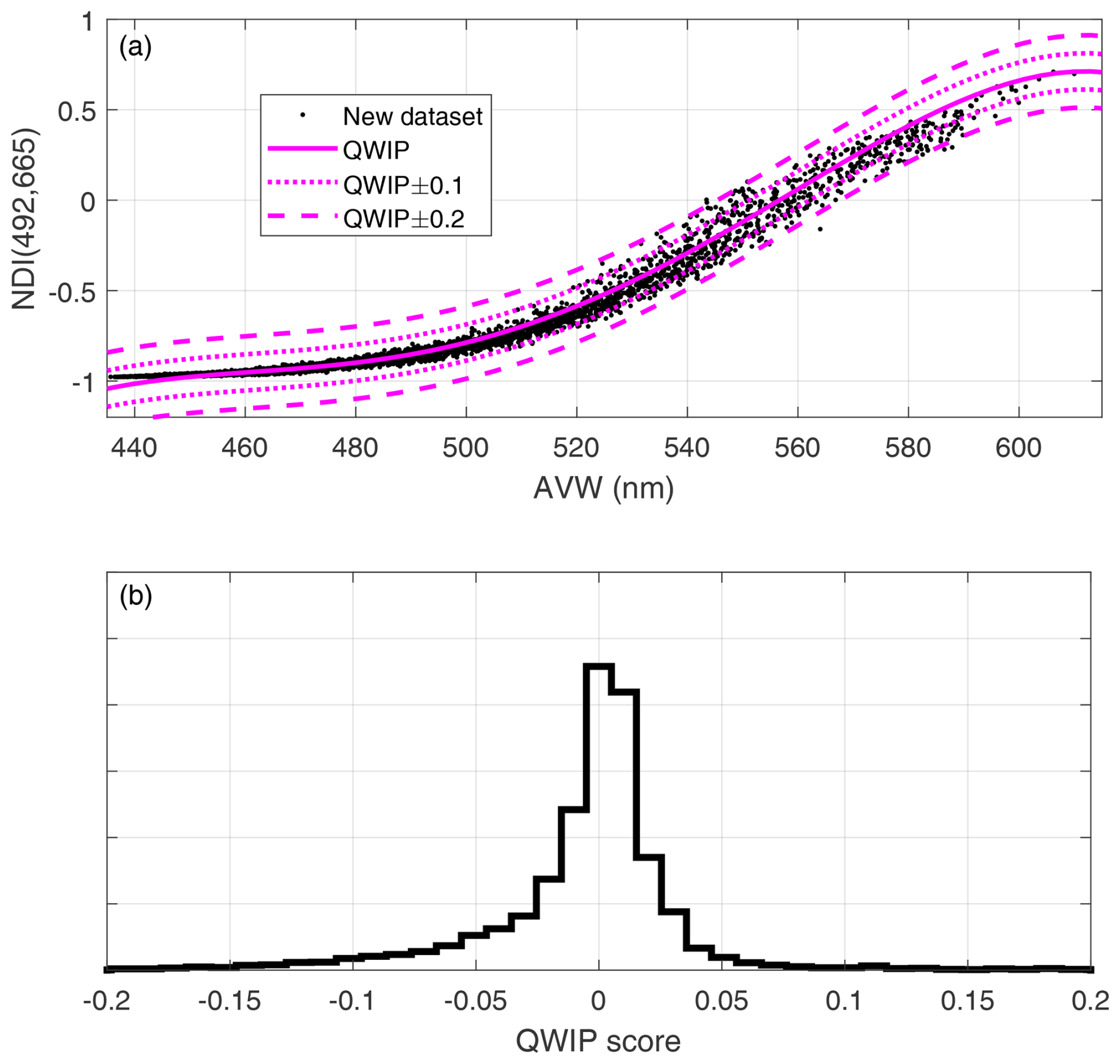
Figure 17 (a) Scatterplot between the apparent optical wavelength (Vandermeulen et al., 2020) and the normalized difference index (NDI) index: $\text{NDI}\left(\mathrm{492}\mathrm{665}\right)=\frac{R_{\mathrm{rs}}\left(\mathrm{665}\right)-R_{\mathrm{rs}}\left(\mathrm{492}\right)}{R_{\mathrm{rs}}\left(\mathrm{665}\right)+R_{\mathrm{rs}}\left(\mathrm{492}\right)}$. Magenta lines represent the QWIP score (Dierssen et al., 2022) and error bars. (b) Histogram of the QWIP score, defined as the difference with respect to the QWIP curve.

The next assessment helps to verify the covariability between R_rs and the absorption coefficient. A one-dimensional predictor χ is derived from R_rs (Lee et al., 2002) as in Eq. (20):

$$\begin{array}{}\text{(20)}& \mathit{\chi }={\log }_{\mathrm{10}}\left({\displaystyle \frac{R_{\mathrm{rs}}\left(\mathrm{443}\right)+R_{\mathrm{rs}}\left(\mathrm{490}\right)}{R_{\mathrm{rs}}\left(\mathrm{560}\right)+\mathrm{5}\frac{R_{\mathrm{rs}}^{\mathrm{2}}\left(\mathrm{665}\right)}{R_{\mathrm{rs}}\left(\mathrm{490}\right)}}}\right).\end{array}$$

This χ index is matched to the non-water absorption spectrum at 560 nm a_nw(560). There are several open-access, freely available in situ datasets that contain both measured variables matched together, such as Valente et al. (2022); Zibordi and Berthon (2024); and PACE Schaeffer, Mouw, and Biosope datasets (Casey et al., 2020). Figure 18 clearly shows the excellent average overlap between our SD and measured data besides differences due to the difficulties of measuring very low absorption. Different bio-optical characteristics produce slight deviations from the mean trend, indicating natural variability.

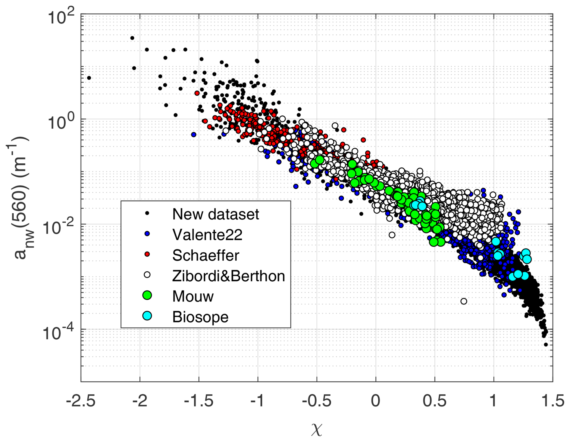
Figure 18 A scatterplot between the R_rs-generated χ index and the matched non-water absorption spectrum at 560 nm a_nw(560). Black dots are from the SD and colored dots are from field data from various references (see text).

A typical benchmark is shown next, where a given chlorophyll concentration in the SD is related to the generated R_rs through the maximum band ratio, MBR_OC4, an index that is used to estimate chlorophyll in the ocean, defined in Eq. (21):

$$\begin{array}{}\text{(21)}& {\mathrm{MBR}}_{\mathrm{OC}\mathrm{4}}={\displaystyle \frac{\max [R_{\mathrm{rs}}\left(\mathrm{443}\right),R_{\mathrm{rs}}\left(\mathrm{490}\right),R_{\mathrm{rs}}\left(\mathrm{510}\right)]}{R_{\mathrm{rs}}\left(\mathrm{560}\right)}}.\end{array}$$

This index has been also used to study the consistency of a given SD in all kinds of water (Nechad et al., 2015). Here, matched MBR_OC4 and chlorophyll concentration from two large in situ datasets is plotted (Valente et al., 2022; Zibordi and Berthon, 2024), showing a good general overlap, though with some degree of differences among them that are explainable due to a different bio-optical characteristics of the seas sampled (Szeto et al., 2011). Data from our SD generally agree with the trend, which essentially shows high linearity in the middle section while saturating at the extremes due to loss of sensitivity. The data cloud of the SD also displays a spread that embraces the in situ datasets used for comparison, suggesting that the optical variability in the in situ datasets is well represented.

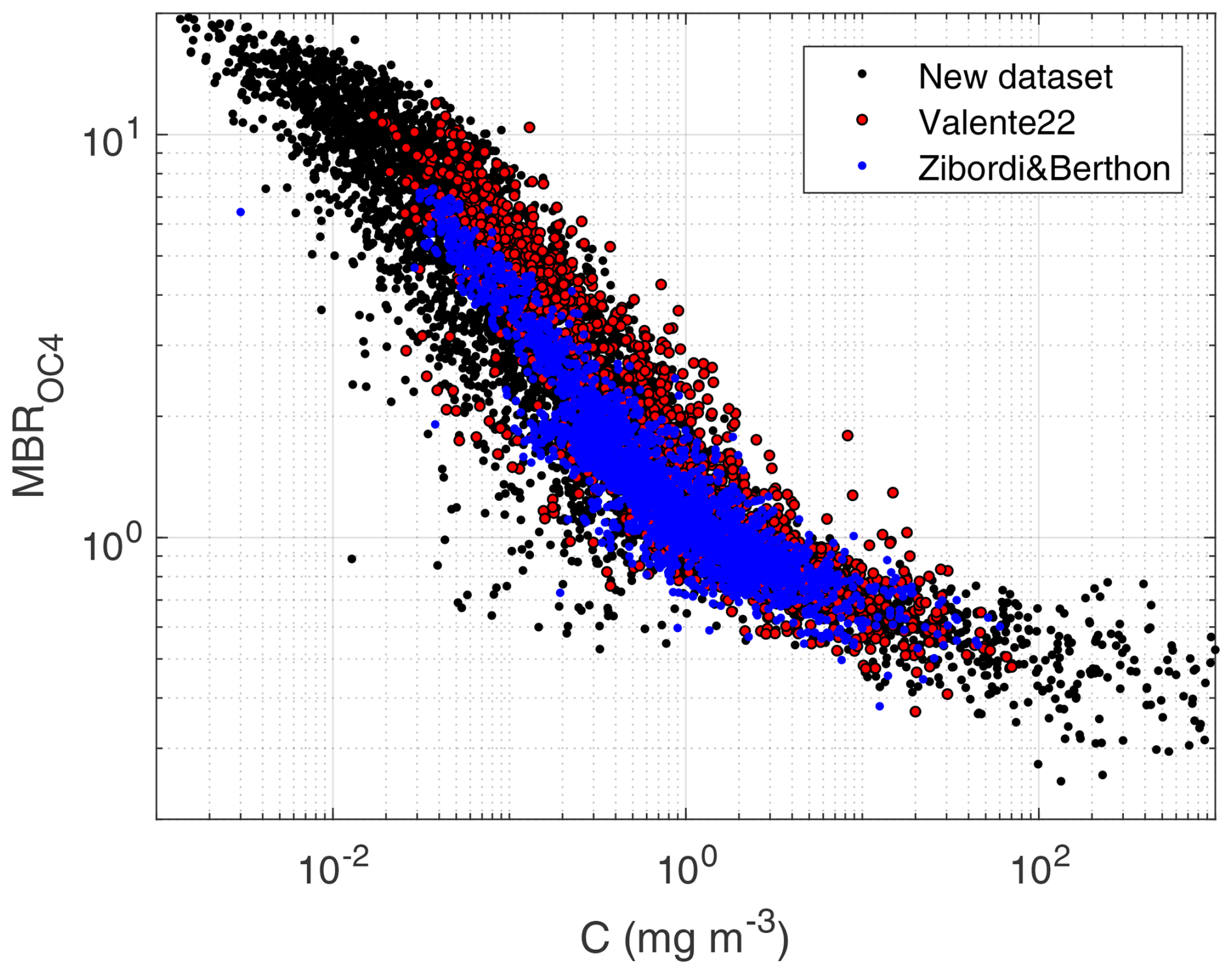
Figure 19 Chlorophyll concentration as a function of the maximum band ratio for OC4-type algorithms for the SD and for data in Valente et al. (2022) and Zibordi and Berthon (2024).

The last comparison to real R_rs data involves the relationship to the total suspended matter concentration (T), a relevant parameter for coastal and inland water studies, which usually show higher turbidities. Interestingly, this involves the absolute value of R_rs and not ratios. In particular, it is known that T covaries with R_rs at long wavelengths and that 665 nm is commonly employed due to the lesser disturbance by CDOM. Our SD does not use T for its generation, so the estimation $T=N+\mathrm{0.07}C$ is used, after Brando and Dekker (2003). Figure 20 shows that the new SD follows the same trend as that from in situ datasets (Valente et al., 2022; Zibordi and Berthon, 2024), but also that it displays a level of spread that includes the in situ datasets, once more demonstrating the success in reproducing a range of natural variability.

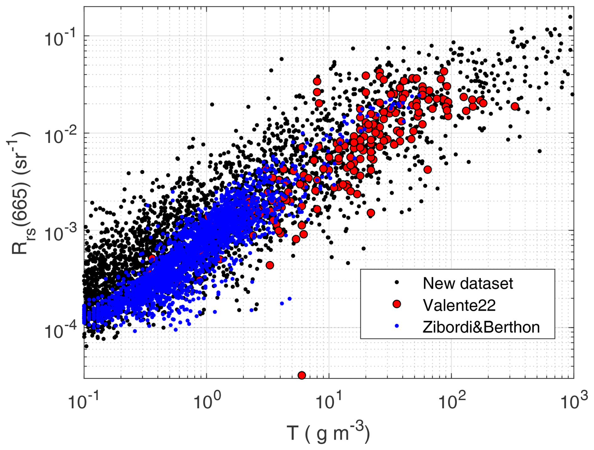
Figure 20 Total suspended matter concentration as a function of R_rs(665) for the SD and for data in Valente et al. (2022) and Zibordi and Berthon (2024).

5 Data file description

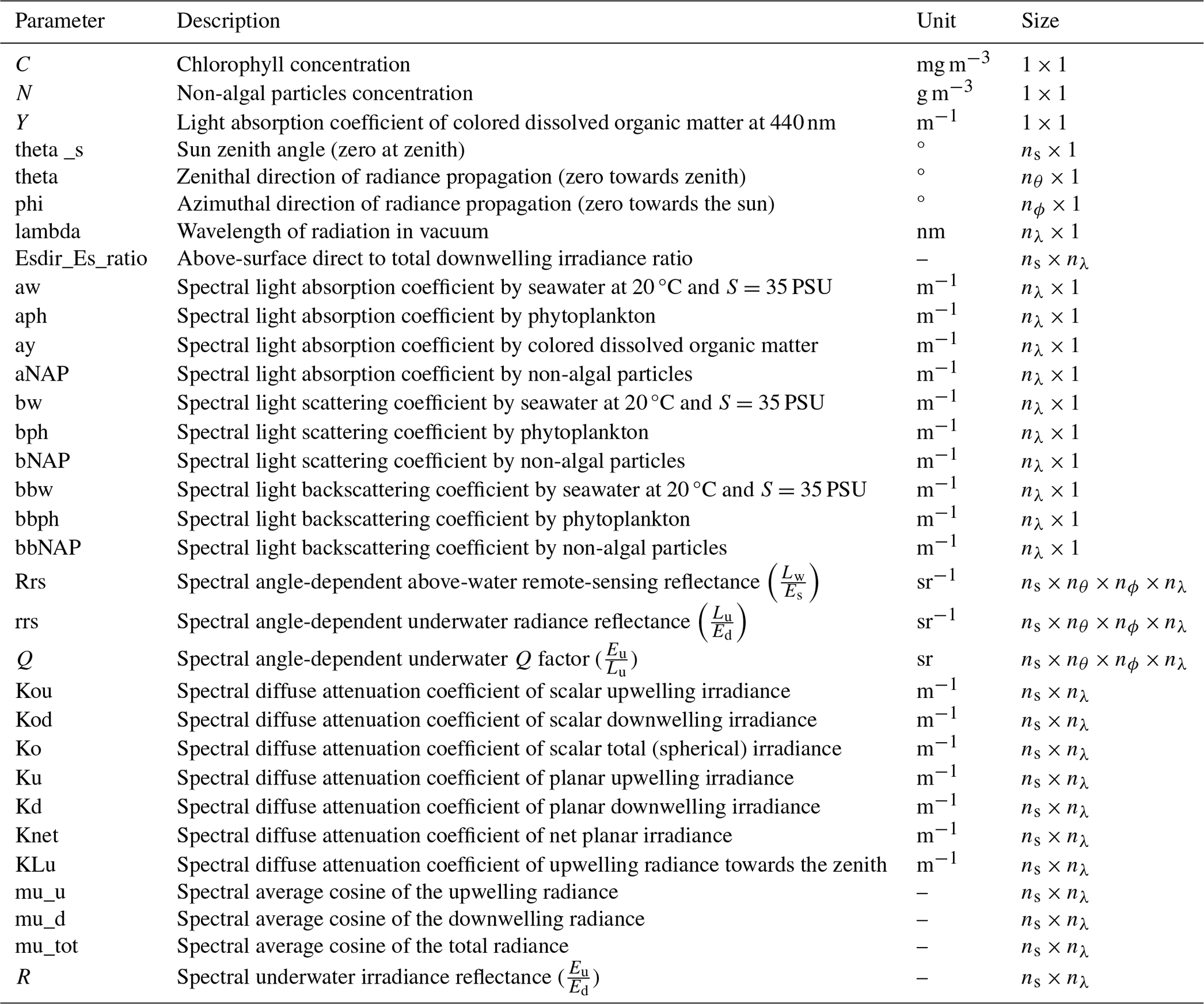
Output data are organized in netCDF files, each containing a given IOP setup and the entire directional AOP output. Table 4 details the file structure. Variables have different sizes, according to their dependence on the following variables that can take the following number of different values: sun zenith angle, θ_s, n_s=10; zenithal direction of radiance propagation, θ, n_θ=10; azimuthal direction of radiance propagation, ϕ, n_ϕ=13; and wavelength of radiation in vacuum, λ, n_λ=451. All in-water AOPs refer to zero depth, just below the surface. Diffuse attenuation coefficients instead required the choice of two close depths to approximate the depth derivatives, which were 0 m and 1 cm as set by default in HydroLight.

Table 4 File description.

6 Data availability

Data described in this paper are freely accessible from Zenodo at https://doi.org/10.5281/zenodo.11637178 (Pitarch and Brando, 2024). The repository hosts two versions of the dataset: one hyperspectral, from 350 to 900 nm, in steps of 1 nm, and a smaller, multispectral one for the 12 Sentinel-3 Ocean and Land Colour Instrument (OLCI) bands between 400 and 753 nm.

7 Conclusions

The presented dataset fills several gaps as identified in our literature review of publicly available in situ and synthetic datasets. The large quantity and high quality of the in situ data allowed for the application of stringent quality control procedures to develop novel bio-optical relationships involving parameters that model absorption and scattering of the optically active constituents. The spread in the data clouds used for bio-optical modeling was reproduced as probability density functions, resulting in a realistic depiction of the natural variability of the in situ data. Validation exercises were provided for the remote-sensing reflectance, showing consistency with the benchmark in situ datasets for every example. Our dataset is therefore representative of natural waters of varying trophic levels and optical complexity. It can be assumed that the underlying bio-optical relationships will become a reference for future optical studies.

Apparent optical properties are resolved at all geometric angles available by the radiative transfer simulations, making this one the first directional dataset ever published. This detail makes it suitable for directional studies of reflectance, diffuse attenuation, and any other derived quantity. The dataset, in its hyperspectral and multi-angular format, is relevant for bio-optical and directional studies applied to current satellite-borne sensors such as OLCI and to next-generation missions such as PACE and CHIME.

The synthetic dataset is distributed in netCDF format as a single file for each IOP case, enabling efficient space management as well as straightforward handling with software packages. Despite the very fine spectral step of 1 nm between 350 and 800 nm and the fact that each file contains the IOP setup as well as all directional AOPs for all 1300 angular configurations (hemispheric variables such as K_d are included for all 10 sun zenith angles), each of the 5000 files is only approximately 5700 kB in size.