A typology of global relief classes derived from digital elevation models at 1 arcsec resolution

Understanding land surface morphology and its relief components, which record the dynamics of the planet's evolution and interaction of multiple environmental factors, constitutes a critical aspect of Earth system science. Advances in Earth observation technologies have enabled access to higher-resolution data, e.g. remote sensing imagery and digital elevation models (DEMs). However, classified relief and landform data with a resolution of approximately 1 arcsec (approximately 30 m) are lacking at the global scale, which limits the progress of related studies at finer scales. Here, we propose a novel framework for global relief classification and release a unique dataset called global relief classification (GRC), which incorporates a comprehensive set of objects that constitute the range of terrains and landforms on Earth. Constructed from multiple 1 arcsec DEMs, GRC covers the global land and ranks among the highest-resolution global geomorphic datasets to date. Its development integrates land surface ontologies, with cores, transitions and boundaries, and key derivatives to strike a balance between mitigating local noise and preserving valuable landform details. GRC categorizes Earth's land relief into two levels, yielding raster files and discrete vector units that record relief type and distribution. Comparative analyses with previous datasets reveal that GRC better captures details of surface morphology, enabling a more precise depiction of geomorphological boundaries. This refinement facilitates the identification of finer and more precise spatial disparities in landform patterns than before, exemplified by marked contrasts between Asia and other continents, and highlights the distinct prominence of Peru and China in terms of relief diversity. Given that the data resolution of GRC accords well with accessible remote sensing imagery and other Earth science datasets, it is readily incorporated into analytical workflows, exploring the relationship between land morphology, surface runoff, climate, and land cover. The full dataset is available on the Deep-time Digital Earth Geomorphology platform and from Zenodo (https://doi.org/10.5281/zenodo.15641257, Yang et al., 2024).

1 Introduction

Understanding the morphology of Earth's surface and its constituent types is one of the fundamental tasks of Earth system science (Evans, 2012; Pepin et al., 2022). In this domain, surface relief is a significant characteristic, playing a critical role in regulating energy flows and material transport across terrestrial environments and exerting a significant influence on geomorphic evolution, hydrological balance, and human activity (Thornton et al., 2022; Viviroli et al., 2020; Xiong et al., 2023; Zhou and Chen, 2025). Although different disciplines may adopt varying terminologies, such as “landform”, “terrain”, or “relief class” (Drăguţ and Eisank, 2012; Meybeck et al., 2001; Thornton et al., 2021; Viviroli et al., 2020), to describe these morphological features, their conceptual essence remains broadly consistent: to represent the spatial patterns of vertical variation that shape Earth's surface and influence key environmental processes. Classifying and mapping Earth's surface into relief classes according to morphological characteristics is a primary means of understanding surface patterns and processes on planet Earth (MacMillan and Shary, 2009; Evans, 2012; Xiong et al., 2022), and advancement in this field has potential benefits for more efficient allocation of global resources to promote sustainable development (Dramis, 2009).

Traditional mapping of relief classes primarily relies on manual interpretation, surveys based on fieldwork, and topographic maps and aerial photographs supported by field investigations (Drăguţ and Blaschke, 2006; Hammond, 1954; Iwahashi et al., 2018; Pennock et al., 1987). A series of technological developments has facilitated automation classification in recent decades, which is largely dependent on topographic derivatives calculated from digital elevation models (DEMs), such as slope, aspect, relief, curvature, and roughness (Jasiewicz and Stepinski, 2013; Amatulli et al., 2018, 2020; Dyba and Jasiewicz, 2022; Snethlage et al., 2022). With the development of Earth observation systems and DEM refinement, several global datasets based on this framework have been proposed using various data sources and at different levels of spatial resolution (Florinsky, 2017; Iwahashi and Yamazaki, 2022). Using a decision tree algorithm and 1 km Shuttle Radar Topography Mission (SRTM) data, Iwahashi and Pike (2007) generated a global terrain classification gridded dataset containing 16 undefined topographic types determined by slope gradient, local convexity, and surface texture. Relying on elevation and the standard deviation of elevation, Drăguţ and Eisank (2012) adopted an object-based method to automatically classify global landforms from SRTM data resampled to 1 km. Meanwhile, Iwahashi et al. (2018) improved their previous work and established 15 classes based on the MERIT DEM. To further eliminate issues involved in detecting narrow valley bottom plains, metropolitan areas, and slight inclines in otherwise largely flat plains, Iwahashi and Yamazaki (2022) introduced the elevation above the nearest drainage line measure and achieved a land surface classification based on a DEM at 90 m resolution. In addition, at regional and global scales, several researchers have achieved automated classification methods following the Hammond procedure (Gallant et al., 2005; Karagulle et al., 2017; Martins et al., 2016). All of these datasets have provided valuable resources for exploring surface patterns and have also played important roles in supporting related disciplines such as hydrology, pedology, and ecology.

However, shortfalls remain in current relief and landform classification research and require attention to the following points. Firstly, most previous studies have adopted relatively coarse-resolution DEMs, resulting in an inaccurate depiction of morphological information. Recent developments in Earth observation technology have concentrated on the deployment of DEMs, which contain abundant geometric information on surface relief (Drăguţ and Eisank, 2011), although the approach and methods for implementing relief classification have not kept pace with advances in DEM resolution and quality. Higher DEM data resolution can be regarded as a double-edged sword, in that it provides the opportunity for relief class mapping at a finer scale while at the same time increasing the challenge of reducing the negative effect of the data noise and abrupt terrain variations (Jasiewicz and Stepinski, 2013) and maintaining the morphological integrity of the identified objects. Secondly, at the global scale, diverse and complex environmental factors increase the complexity of the land surface morphology, which poses substantial challenges to the generalizability of classification methods (Li et al., 2020). With increasing human impact on the land surface, a re-evaluation of relief and landform classification that takes advantage of an increasingly potent digital database and ongoing improvements in human understanding of land surface morphology seems opportune. Finally, geomorphic information obtained from a particular metric is derived at a particular spatial scale, determined jointly by the DEM resolution and window size in the neighbourhood analysis, giving rise to uncertainties in the classification results.

Therefore, the development of innovative classification approaches and systems based on high-resolution DEMs remains a priority for research on global relief classes and landforms. In this study, we conduct a classification and mapping of global relief classes based on a DEM at 1 arcsec resolution. We focus on the classification of geomorphic objects that emphasizes morphological differences and, in so doing, we present the practical expression of object ontology at the global scale that offers valuable insights into Earth's surface structure comprising the constellation of relief types and their boundaries. The objectives of this research are (1) to construct a global classification system and framework for land relief classes to integrate domain consideration of landform-related studies, (2) to develop an automated classification and mapping model for global relief classes, and (3) to make available a comprehensive global dataset of relief units.

2 Methodology

2.1 Hierarchical classification system and data

In aiming to provide a comprehensive classification of relief and landform classes at the global scale, our study encompasses all terrestrial regions worldwide, including islands and polar areas. Identifying objects and constructing a classification system are preliminary and significant steps in related studies. It is crucial to recognize that land surface objects not only represent assemblages of quantitative characteristics but also convey basic human understanding of nature (Smith and Mark, 2001). For example, the identification of what is acknowledged as a “mountain” is as much a product of human perception as of its natural characteristics (Smith and Mark, 2003), thus emphasizing the importance of incorporating human understanding and domain application into relief classification and mapping. In this study, we focus on the classification of relief classes that emphasize vertical variation and relief intensity across different landforms that are not only perceptible to humans but also constitute vital components in the analysis of surface environments.

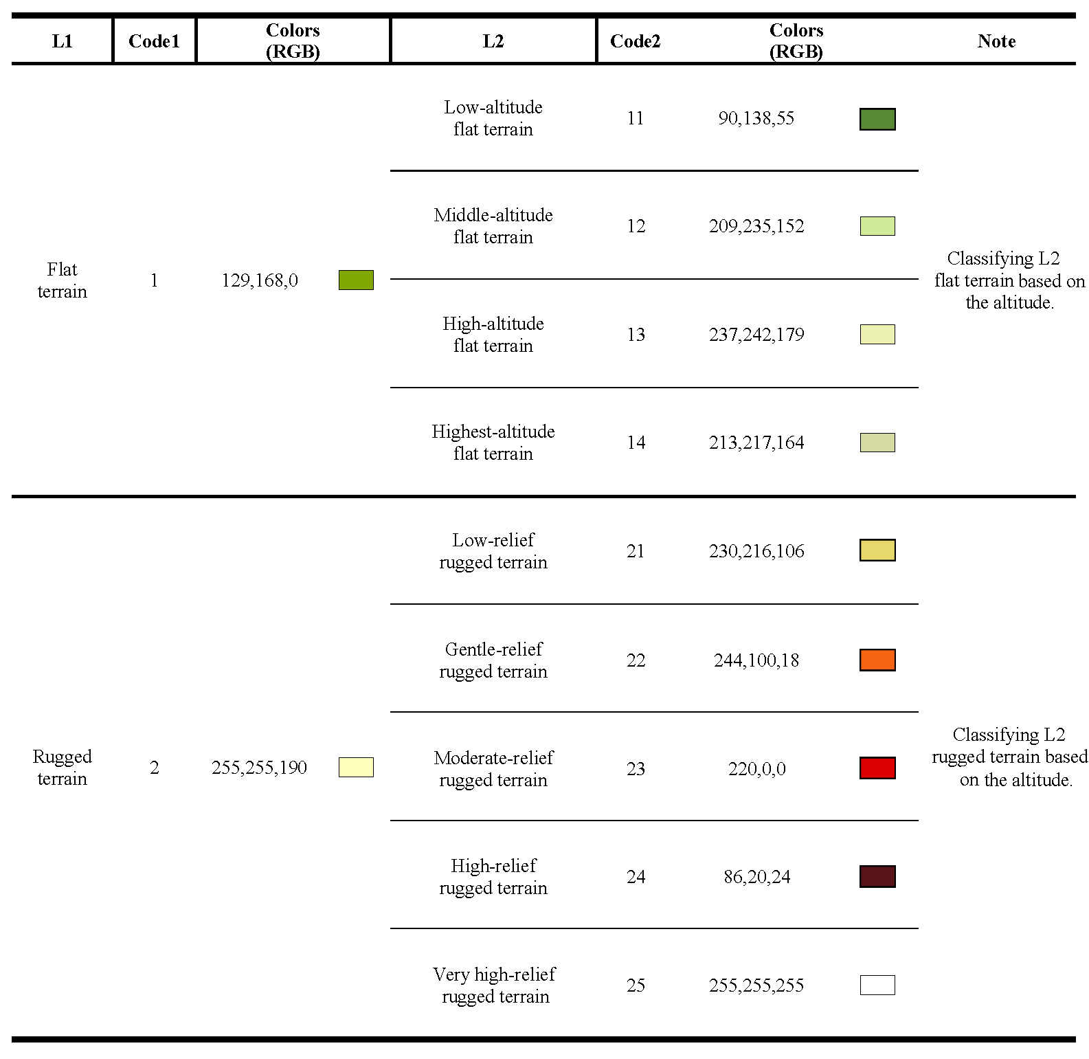
In taking into consideration the complexity of global topographic characteristics, the classification criteria should satisfy the following requirements: (1) the determined classes should be globally applicable, (2) the setting of relief classes should conform with the current knowledge domain of Earth system science, and (3) specific criteria should be able to be interpreted and applied. After comprehensive consideration of previous classification systems (Meybeck et al., 2001; Zhou et al., 2009), we propose a set of criteria for relief classification. The new criteria integrate the typical rules of relief and landform classification with indices proposed in this work and are aimed at reflecting human knowledge in a quantitative way. We establish a hierarchical classification system comprising two levels and nine classes (Table A1), thereby advancing a structured framework for understanding Earth's diverse landscapes. The first level (L1) corresponds to the conventional concept of a complete landform entity, while the second level (L2) provides progressively finer-scale morphological information. The L1 classification primarily aims to distinguish between broadly distributed rugged uplands and their counterpart – flat lowlands (Meybeck et al., 2001; Viviroli et al., 2020). To ensure clarity and interdisciplinary compatibility, we deliberately avoided using terms in a strict geomorphological sense (e.g. “mountain” or “plain”) and instead adopted extended geographic terms. In this study, we refer to the two primary surface types as flat terrain and rugged terrain, based on their differences in slope characteristics. While flat terrain and rugged terrain largely correspond to traditional concepts of plains and mountains, respectively, they are defined based on quantifiable morphological characteristics, thereby offering a more flexible and reproducible framework. These two contrasting relief classes provide essential support for understanding landform processes, analysing hydrological patterns, and assessing the spatial distribution of human activities across diverse environmental contexts (Viviroli et al., 2020). This classification perspective aids researchers in conducting macroscale studies. At L2, the flat terrain retains elevation-based characteristics and is further divided into low-altitude, middle-altitude, high-altitude, and very-high-altitude flat terrain. Rugged terrain is subdivided at L2 into low-relief, gentle-relief, moderate-relief, high-relief, and very-high-relief rugged terrain.

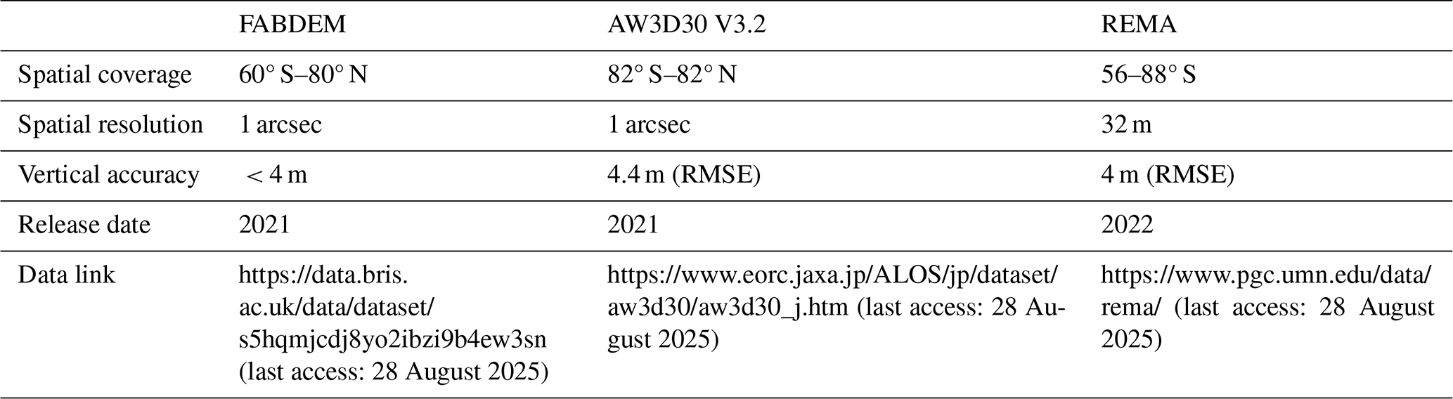
To attain global coverage, we utilize three DEM datasets (Table 1). These datasets are publicly available for access and have been widely used in geomorphological studies, ensuring their accuracy and validity. In this work, the Forest and Buildings removed Copernicus DEM (FABDEM) (Hawker et al., 2022) provides the primary data for latitudes 60° S–80° N. This dataset is the first bare-Earth DEM dataset at a global scale at 1 arcsec (approximately 30 m) resolution, developed using machine learning techniques from the Copernicus DEM. By eliminating the bias resulting from building and vegetation heights, some terrain features, such as slope, aspect, and watersheds, can be estimated more accurately, which is of significant benefit in landform classification. Meanwhile, the Advanced Land Observing Satellite (ALOS) World 3D – 30 m (AW3D30) (Tadono et al., 2014) and the Reference Elevation Model of Antarctica (REMA) (Howat et al., 2022) are used to supply data for the area missing from FABDEM. In addition, to avoid the negative impact of ocean pixels on the classification results, the OpenStreetMap (OSM) Land Polygon was utilized as a mask to eliminate the sea.

Table 1 Data sources and attributes.

2.2 Classification method

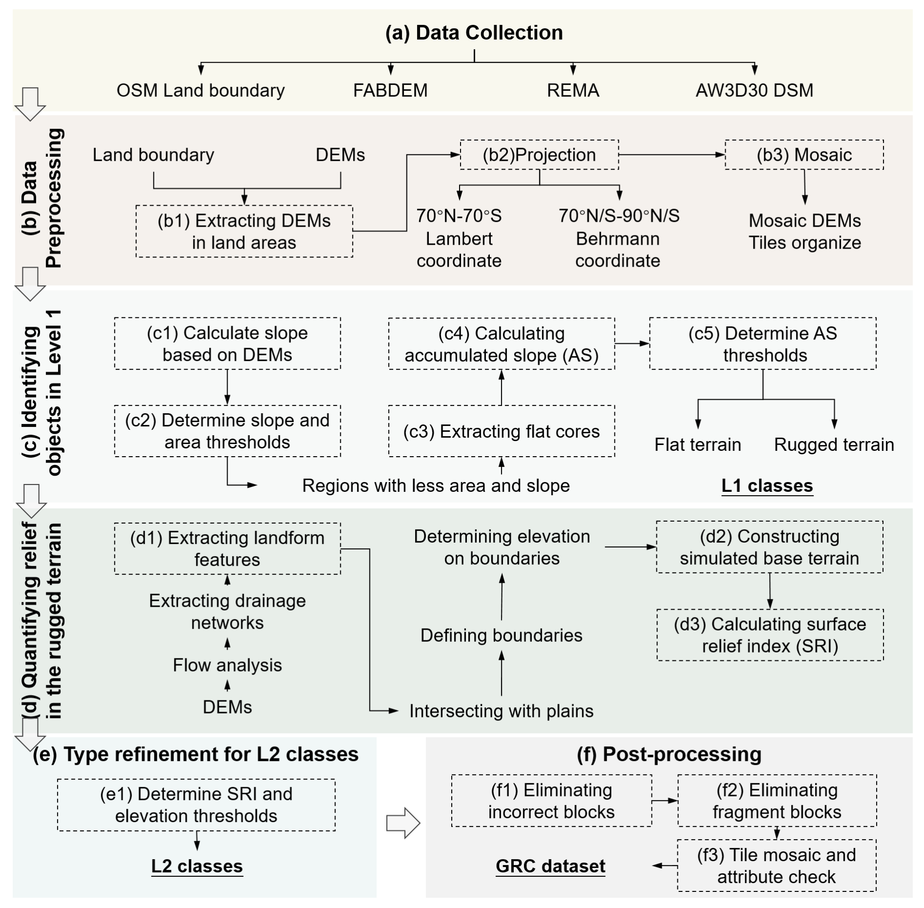
In this study, we propose a new framework and provide the corresponding implementation workflow. The proposed method has a hierarchical structure, involving data pre-processing, identification of mountains and plains, calculation of the surface relief index (SRI), relief classification, and post-processing. Figure 1 illustrates the workflow. The following sections provide details that should allow users to reproduce our results. In this study, we built characteristic quantification and classification models based on tools in ArcGIS Pro. A detailed description of the step-by-step procedures follows below.

Figure 1 Workflow of the proposed classification method.

2.2.1 Data pre-processing

As shown in Fig. 1b, data pre-processing focuses primarily on land area extraction and data merging. We use the OSM Land Polygon as the land mask to eliminate the marine pixels that negatively influence the subsequent processes. To improve the processing efficiency, the original DEM elements with a size of 1 × 1° are mosaicked to tiles of 10 × 10°. Meanwhile, due to the requirement for calculating landform derivatives, we determine the projection principles as follows: tiles between 70° N and 70° S are re-projected into the equal-area Behrmann projection, and tiles polewards of 70° N and 70° S are re-projected into the Lambert azimuthal equal area. To mitigate border effects between the two projection zones, we have implemented an overlapping strategy in our processing. Specifically, we processed the DEMs in 11° × 11° tiles, ensuring that the main 10° × 10° area is used as the final output. This approach helps maintain consistency and minimizes distortions at the transition between the projection zones. For consistency and ease of use, the final TIFF files have been re-projected into a single coordinate system (EPSG:3857).

2.2.2 Identifying objects at Level 1

Identifying and distinguishing contrasting flat and rugged terrain represents the initial step in the proposed framework. To achieve this, we propose re-examining classification from an ontological perspective. In information science, an ontology is a neutral and computationally tractable description of a given individual or category which can be accepted and reused by all information gatherers (Smith and Mark, 2003). In this study, based on spatial information theory, we propose a conceptual description of relief objects that enhances the generalization of land surface and reduces the negative influence of vagueness. Considering that the characteristics of flat terrain are more distinct and their definition is clearer, we will use flat terrain as the foundation for expanding the relief ontology. As shown in Fig. 2a, the conceptual model of flat terrain includes three elements, i.e. core, transition, and boundary. The core represents areas with the most typical flat characteristics, i.e. a very low slope. Transitions occur around cores and contain areas with a higher slope than typical flat terrain, i.e. areas that in part satisfy their classification as flat terrain but also exhibit sloping characteristics not typical of flat terrain. In a general geographic context, these areas should also be classified as flat terrain. However, current methods that emphasize local topographic characteristics often fail to identify them correctly. The boundary is defined as the spatial margin of flat terrain where topographic properties and classification labels shift gradually toward those associated with rugged terrain. In this context, misclassification tends to occur in transitional zones, which exhibit mixed topographic features that do not fully align with either flat or rugged terrain characteristics. We have designed a practical framework based on landform ontology to classify these two objects as shown in Fig. 2.

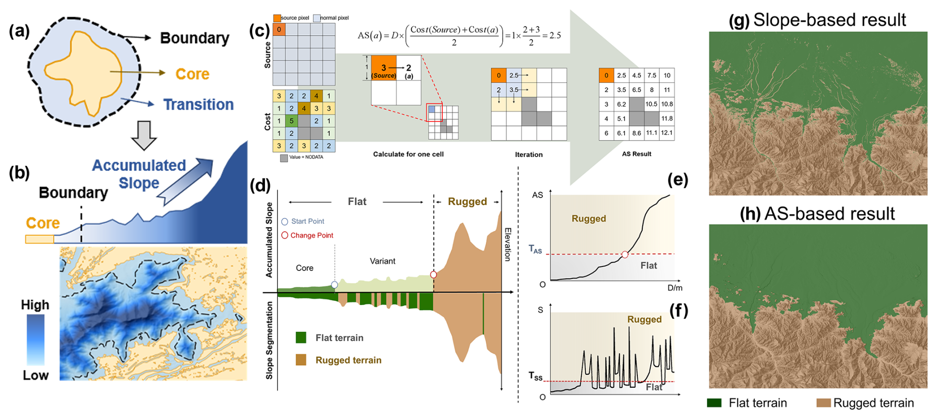
Figure 2 Illustration of the calculation methods. (a) Conceptualization of flat terrain. (b) Calculation principle and results of the accumulated slope (AS). (c) Schematic diagram of the cost–distance algorithm. The cost refers to the slope in this process. (d) Profile reflecting land surface composition according to the proposed conceptual model, segmented based on the slope. (e) Calculated result of the AS and (f) calculated result of the slope, where T_AS is the threshold of the AS and T_SS is the threshold of the surface slope. For panels (c) and (d), areas smaller than the threshold are classified as flat terrain (marked in green), while the remaining areas are classified as rugged terrain (marked in brown). Panels (g) and (h) compare the AS and slope indicators in the division of Level-1 classes.

In conducting the classification, firstly, we regard areas with low slope angles as flat cores. Here, the slope threshold (T_SS) is recommended to be set as 1.5° according to our global pre-assessment experiments. Areas where the slope angle lies below the threshold T_SS are classified as flat cores. A block must be greater than 0.1 km² to be classified as a core area. As noted above, areas beyond the core with relatively low relief should also be considered flat terrain in the geographic sense. However, segmentation based on slope characteristics usually fails to identify them as such due to emphasis being placed on local changes in topography (Fig. 2g). Meanwhile, the resulting landscape segments may themselves contain fragments that reflect local topographic changes but do not represent actual landform objects. It is challenging to correct all such fragments across complex terrain scenarios at the global scale, thus limiting the feasibility of automated global relief classification. To address these issues, as the second step in our classification process, we introduce the concept of an accumulated slope (AS) and develop an AS derivative that quantifies the attributes of transitions by calculating the AS along a path that has the lowest slope cost (Fig. 2b). In this process, the core is as extracted in the previous step, and the cost surface is the slope gradient. The AS is calculated as the minimum cumulative cost of each position to the nearest core along a specific path. In the AS calculation of general positions, this algorithm employs an iteration starting from the cell closest to the cores and follows the calculation principle shown in Fig. 2c to compute the minimum accumulated slope of each cell to the core. The completed area is then expanded until all grids are associated with increasing costs. This process follows the geospatial analysis principle of the minimum accumulated cost (Sechu et al., 2021). The tool of distance accumulation in ArcGIS Pro can perform this calculation. Segmenting landforms through the determination of the thresholds for topographic derivatives is one of the most common methods used in geomorphological studies and transforms qualitative perception into quantitative computation. As shown in Fig. 2d, due to differences in topographic characteristics between flat and rugged terrain, the AS has a low rate of increase in the areas classified as flat terrain and a high rate of increase in rugged areas. This phenomenon facilitates the determination of an appropriate AS threshold, which can be achieved by searching for abrupt changes in the AS profile. In this step, the threshold of the AS (T_AS) is recommended to be 1500–2000 based on the pre-experimental results conducted on numerous samples worldwide. Areas where the AS value is less than T_AS are merged with the cores to form the complete flat terrain, while the remaining areas are classified as rugged terrain. This threshold range is provided as a reference, but gentle adjustments to the thresholds may be required in some special areas, such as small islands, through human–computer interaction. In some cases, such as small islands where traditional watershed and triangulated irregular network (TIN)-based methods tend to struggle, it may exceed the recommended threshold range. Through the above segmentation, we can obtain the boundary of the flat terrain and construct the complete flat area consisting of the core, variant, and boundary. As shown in Fig. 2g and h, this workflow exaggerates the difference between the flat and rugged terrain and converts the local slope into an indicator of global characteristics. This novel method avoids the negative effect of local window analysis and is beneficial for maintaining the landform semantics for each block.

2.2.3 Quantifying surface relief in the rugged terrain

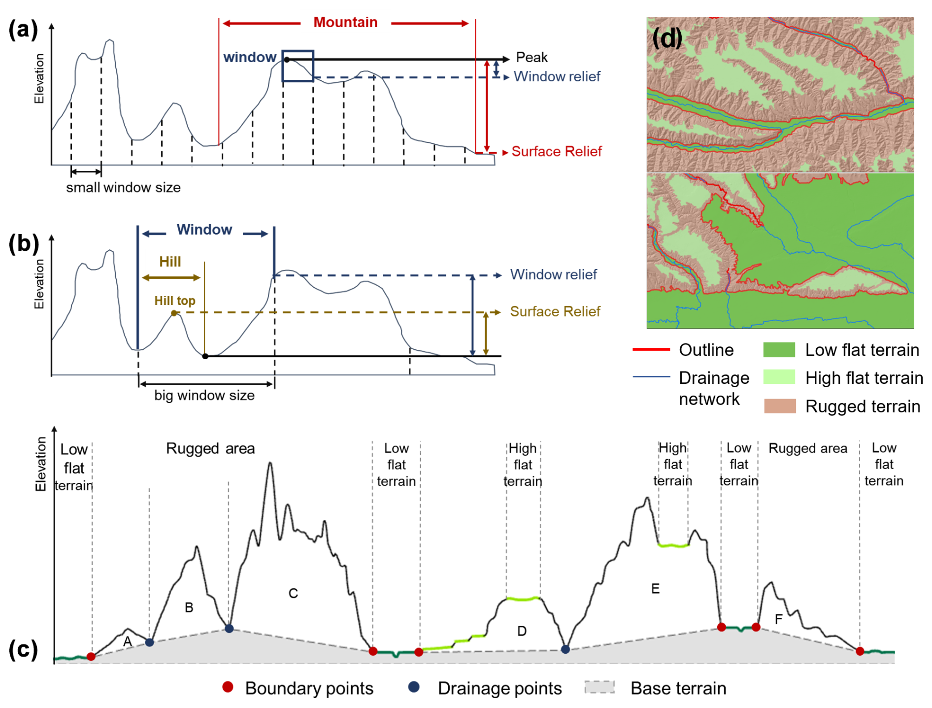
Figure 3 Uncertainty in relief calculation based on the window analysis. (a, b) The relationship between different windows and surface relief in rugged areas. (c) Schematic diagram illustrating the base terrain for calculating the surface relief index. (d) Features used to create TIN and build the base terrain.

In this step, we focus on quantifying relief difference to achieve comprehensive classification of L2 classes. It should be noted that the term “terrain relief” in this study emphasizes the use of quantitative terrain metrics (e.g. the relief index) to measure the degree of vertical variation across Earth's surface. Terrain relief refers to the difference in elevation between the highest and lowest points within a particular spatial unit. This factor significantly influences land surface classification. However, commonly employed indices reflecting topographic relief are found using a window of fixed size such as 3 × 3 pixels, 5 × 5 pixels, or larger (Maxwell and Shobe, 2022), a method which fails to account for geomorphological semantics and which therefore disregards the integrity of a mountain or hill. Window size has a significant impact on the results of relief quantification. As shown in Fig. 3a and b, window analysis tends to disrupt the integrity and continuity of geomorphological elements. Moreover, a small window size is insufficient to capture entire elements, particularly in the case of large mountains, while a large window size may incorporate other elements and fail to capture the real relief effectively. The uncertainty introduced by window size further increases the difficulty of global classification and mapping based on the relief index. Even the multi-scale synthesis approaches can effectively mitigate scale-dependent limitations: these methods still inherently face challenges associated with determining appropriate scale ranges in algorithms.

Therefore, we propose a new method for relief quantification which does not rely on traditional window-based calculation. In this paper, the SRI is defined as the degree of relief relative to the flat areas surrounding rugged terrain. We regard the elevation at the foot of the rugged terrain as the base elevation and then calculate the elevation difference between each position in the rugged terrain and the base elevation. Compared to the traditional method of relief calculation (e.g. the difference in elevation within a particular window size), the SRI considers the vertical elevation differences between the surface and the base, which are more suitable for objectives in landform-related studies such as mountain climate and biodiversity.

This step includes three sub-procedures. Firstly, we constructed the rugged terrain extent as the foundation for subsequent calculation. The flat terrain boundary is primarily used to define the extent of the rugged terrain. However, when the area of rugged terrain (such as mountains) is large and the base elevation is constructed solely from the boundary of the flat terrain, the result may not accurately reflect the actual terrain relief. To refine the representation of surface relief, we introduce linear features representing rivers. These additional lines can be obtained through DEM-based hydro-analysis (Li et al., 2021). In order to ensure that flat terrain at high elevations does not interfere with the definition of the rugged unit, since it is, in effect, part of the rugged terrain range (Fig. 3c), we exclude high-altitude flats (marked in light green in Fig. 3d) that have no fluvial features in order to retain the integrity of the associated rugged terrain range. Figure 3d shows the final elements involved in establishing the base elevation, which corresponds to the boundary of the low-altitude flats and fluvial features (marked in red in Fig. 3d). Secondly, we constructed the base elevation to support the calculation of the SRI. In this case, the rugged terrain extent, which replaces the analysis window in traditional relief calculation, is used to construct the base elevation. Specifically, we construct the TIN based on the position extracted in the first step and then regard the elevation value in the TIN as the base elevation. The construction of the TIN can be achieved in ArcGIS Pro. Thirdly, the SRI is obtained by calculating the difference between each cell altitude and its corresponding base elevation. This novel method provides a more appropriate representation of the underlying terrain.

2.2.4 Type refinement for L2 classes

According to the results of previous studies (Meybeck et al., 2001; Zhou et al., 2009), we constructed the classification criteria shown in Table A1 in the Appendix. For flat terrain, we use altitudes of 1000, 3500, and 5000 m as break points to generate the low-, middle-, high-, and highest-altitude classes. Rugged terrain is classified as low-relief, gentle-relief, moderate-relief, high-relief, and very-high-relief classes, based on threshold SRI values of 200, 1000, 3500, and 5000 m. Overall, this yields six classes in L2.

2.2.5 Post-processing

Following the completion of the above processes, a map is generated that includes all the basic relief classes. However, due to interference caused by the existence of locally steep changes in topographic relief, this output still contains some features in the flat areas misclassified as rugged terrain. Meanwhile, although the data we used have high resolution and good quality, outliers and data noise remain. Such anomalies may result in small blocks with relatively low terrain relief. In accommodating this limitation, we designed an optimization process to correct these misclassifications. We used area and SRI to reflect their characteristics (e.g. fragmented and relatively low relief). Considering the application of geomorphological data and the resolution of fundamental data, we determined that our study corresponds approximately to the equivalent of 1:200 000 geomorphological mapping. Under the conditions of the 1:200 000 scale, the minimum displayable patch size is approximately 0.16 km². The SRI threshold is derived from Zhou et al. (2009), who defined plains as blocks with reliefs less than 30 m. Therefore, blocks with areas of less than 0.16 km² and SRIs below 30 m are regarded as misclassified blocks, which are then integrated as part of the surrounding flat terrains.

Meanwhile, we designed an additional step to optimize the results for desert areas. Many arid regions are characterized by dunes, which are distinctive aeolian landforms of varying shapes and sizes constructed from unconsolidated sand (Hugenholtz et al., 2012). Dunes are generally smaller in scale than mountains, and this challenges our approach to relief classification (Shumack et al., 2020), increasing the difficulty of accurate dune mapping. In this study, we regarded sand dunes as low-relief rugged terrain due to their morphological similarity. However, the variation of dune size and shape poses significant challenges to the accuracy of dune classification in the current unified framework. Therefore, we design an optimization step to correct the classification results in which dunes and inter-dune areas are separated and identified according to their altitude and SRI. Firstly, on the basis of their geomorphological characteristics, remote sensing images, and hillshade maps, we demarcated the major global sand desert regions. Secondly, we used the DEM to extract the topographic feature lines by surface analysis of extraction of desert feature lines. Employing the SRI calculation as for the other regions, we then constructed the base terrain. In this case, the drainage networks were extracted with the threshold T_D1 of 20 000, and then we extracted sampling points from these networks to construct TINs. We calculated the SRI and then set the segmented threshold T_D2. Due to inconsistencies in the scale of dunes worldwide, we applied an adjustable T_D2 ranging from 2 to 10 m. Areas less than T_D2 are defined as inter-dune (equivalent to plains in the basic landform classification). All patches smaller than T_D3 0.02 km² were regarded as fragments and integrated into the surrounding vector blocks. Finally, we employed the smoothing tool to ensure the appropriateness of their boundary.

3 Results and discussion

3.1 Global relief classification results

Figure 4 shows the global relief classification (GRC) results based on the abovementioned framework. This hierarchical dataset provides a more comprehensive understanding of Earth's surface. To visualize the results in detail, three typical regions are selected to demonstrate the performance of the GRC dataset. Figure 5 shows GRC in typical regions and the corresponding remote sensing images from Esri world imagery. The selected regions contain examples of the main land surface on Earth as well as transition areas of different relief classes. In mountainous areas, as shown in Fig. 5a, rugged terrain range and valley orientation are clearly discernible, which together form the fundamental structure for expressing mountains. GRC clearly illustrates the transition zones between mountains (represented by rugged terrain) and plains (represented by flat terrain) as well as potential floodplains. While such phenomena are visually discernible in remote sensing imagery, using our proposed framework, they are extracted based on quantified morphological characteristics. The abundant information on landform composition provided by GRC can facilitate study of areas with high geomorphological value, such as fjords (Fig. 5b). In desert areas (Fig. 5c), GRC effectively illustrates the transitional patterns between dunes and depressions. Based on abundant morphological characteristics, GRC can depict sand dune boundaries that are strikingly consistent with those visible in the imagery. This further underscores the performance of GRC in capturing detailed geomorphic features across varied terrains.

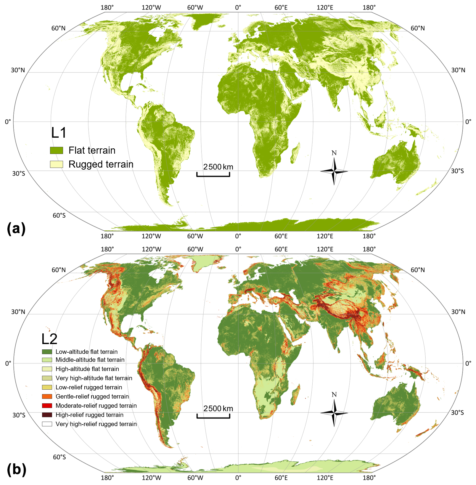
Figure 4 Results of the global relief classes with 30 m resolution. Panels (a) and (b) represent the L1 and L2 classes, respectively.

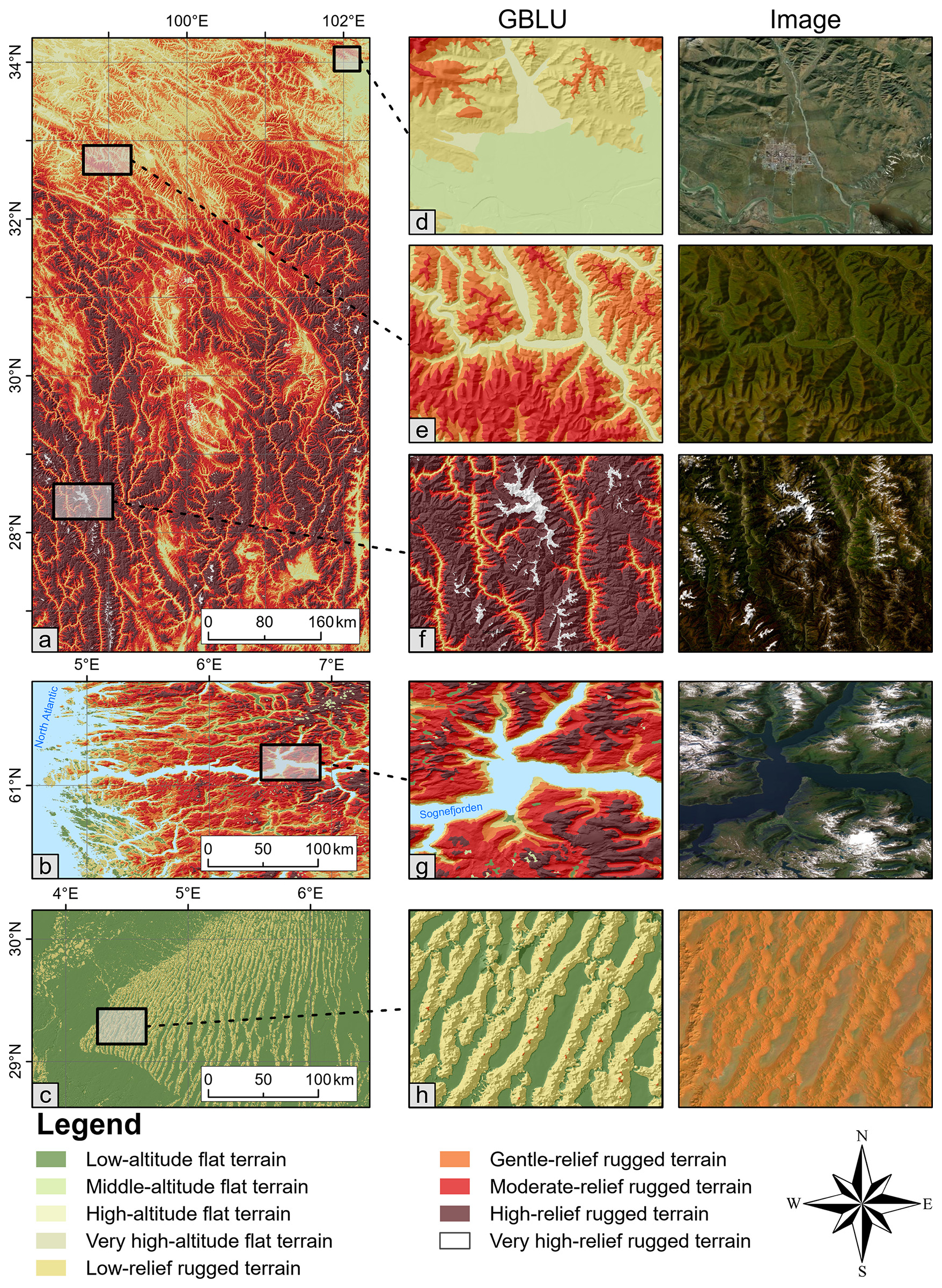
Figure 5 Comparison of the classification results constructed in this paper, together with the remote sensing imagery. (a) Eastern part of the Tibetan Plateau. (b) The fjord coast in western Norway. (c) Desert area in the central Sahara. Panels (e)–(h) are local enlarged areas.

3.2 Result comparison and validation

We conducted comparisons between the GRC dataset and multiple other datasets (including landform, terrain, and relief classification) to comprehensively evaluate our results. The most significant improvement achieved by applying GRC is the increased detail in representing terrain features. The GRC-based classification markedly enhances the delineation of independent landforms, such as dunes and mountains, which have clear boundaries and serve as key elements in the analysis of spatial structures and interactions. Meanwhile, valley-like objects can also be reflected by GRC. The classification systems of Drăguţ and Blaschke (2006) are similar to GRC but have a coarser resolution of 1 km, making them less effective at capturing terrain details. Figure 6 illustrates that there is a variation in the understanding of landform types among different scholars. As noted above, Iwahashi's results align more closely with terrain classification systems in capturing slope features, such as flow channels on volcanic flanks, which occur at finer spatial scales than the terrain objects represented by GRC. It is worth noting that, as illustrated in Fig. 6e, the incorporation of the SRI leads to the classification of dunes into three distinct sub-classes: ridge, slope, and inter-dune. While this finer-level classification provides enhanced information on relief variations, it may be perceived as compromising landform integrity in certain application contexts. Therefore, we recommend that users select either the L1 or L2 classification level, depending on their specific research or application needs in desert areas.

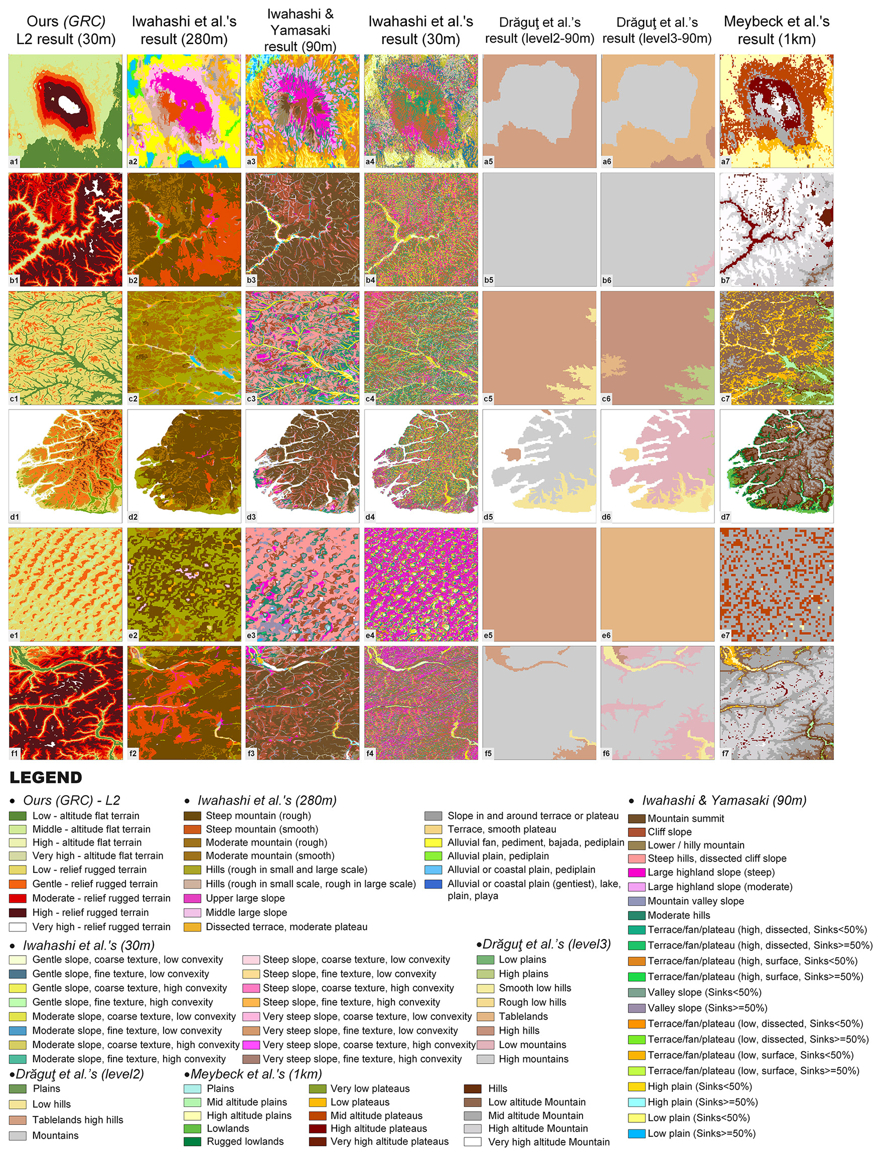
Figure 6 Comparison of GRC with other classification results. The selected study areas, from top to bottom, are as follows: (a) Kilimanjaro, (b) Namcha Barwa in the Himalaya, (c) the Greater Khingan Mountains, (d) fjords in New Zealand, (e) the Badain Jaran Desert, and (f) the Central Alps.

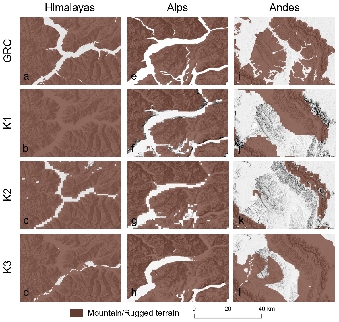
Figure 7 Comparison between GRC and three mountain definitions presented in the Global Mountain Explorer (https://apps.usgs.gov/glbeco/gme.html, last access: 28 August 2025).

We conducted a more detailed comparison of mountain regions with the Global Mountain Explorer (GME). The GME dataset contains three subsets using the DEM with spatial resolutions of 1000, 1000, and 250 m to generate global mountain maps. These three datasets (i.e. K1, K2, and K3) are produced by analysing the morphological derivatives using a moving neighbourhood analysis window for derivative calculation (Kapos et al., 2000; Karagulle et al., 2017; Körner et al., 2011). Differences in application objectives and the selection of input variables have led to notable discrepancies between the classification results of the three datasets. K1 was established to support the global mapping of mountain forests by identifying mountainous regions where a combination of elevation, slope, and terrain ruggedness exceeds certain threshold values. K2, aimed at enabling comparative studies of mountain biodiversity, employed a comparable methodology but relied exclusively on ruggedness as the determining factor. Meanwhile, K3 emerged from efforts to construct a global ecosystem map in which mountainous areas were defined by extracting this particular category from a broader classification of “ecological land units” (Sayre et al., 2018; Thornton et al., 2022). As shown in Fig. 7, the GRC dataset clearly outperforms the other three datasets in depicting mountain details, especially valleys. This can be seen in Fig. 7a–h, where the K1, K2, and K3 data exhibit separated upland blocks in mountainous regions with complex and intense terrain variations and fail to represent continuous valleys.

3.3 Continental and national compositions of relief classes

We used a cell size of 100 m × 100 m to accurately assess the proportions of GRC L2 classes across continents worldwide, thereby yielding insights into their spatial variations. Our re-quantified global distribution of relief classes provides the most detailed estimates to date of the proportion of flat and rugged terrain. Asia exhibits a very distinctive pattern, since flat terrain covers only 59 % of its area, the lowest among all of the continents, while there is a significantly higher proportion of rugged terrain, consistent with its pronounced topographic diversity. Africa is characterized by the dominance of extensive flat terrain in terms of relative area. However, in absolute terms, Asia contains a significantly larger extent of flat terrain, exceeding that of Africa by approximately 4.1 % (Fig. 8b). Compared to the global scale, the presence of continental marginal mountain chains results in a significantly lower proportion of flat terrain and a correspondingly higher proportion of rugged terrain in both North and South America. We further conducted a comprehensive analysis of relief classes and their proportions at the national and regional scales across all countries and regions worldwide to reveal patterns of variation. Figure 8c illustrates the proportion of L2 classes in the top 30 countries ranked by area, while Fig. 8d depicts the standardized proportion of the relief classes within these countries, sorted based on the proportion of low-altitude flat terrain. China contains a significantly high proportion of rugged terrain, indicating its diverse and rugged landform composition, while Peru contains the lowest proportion of flat terrain (40.5 %).

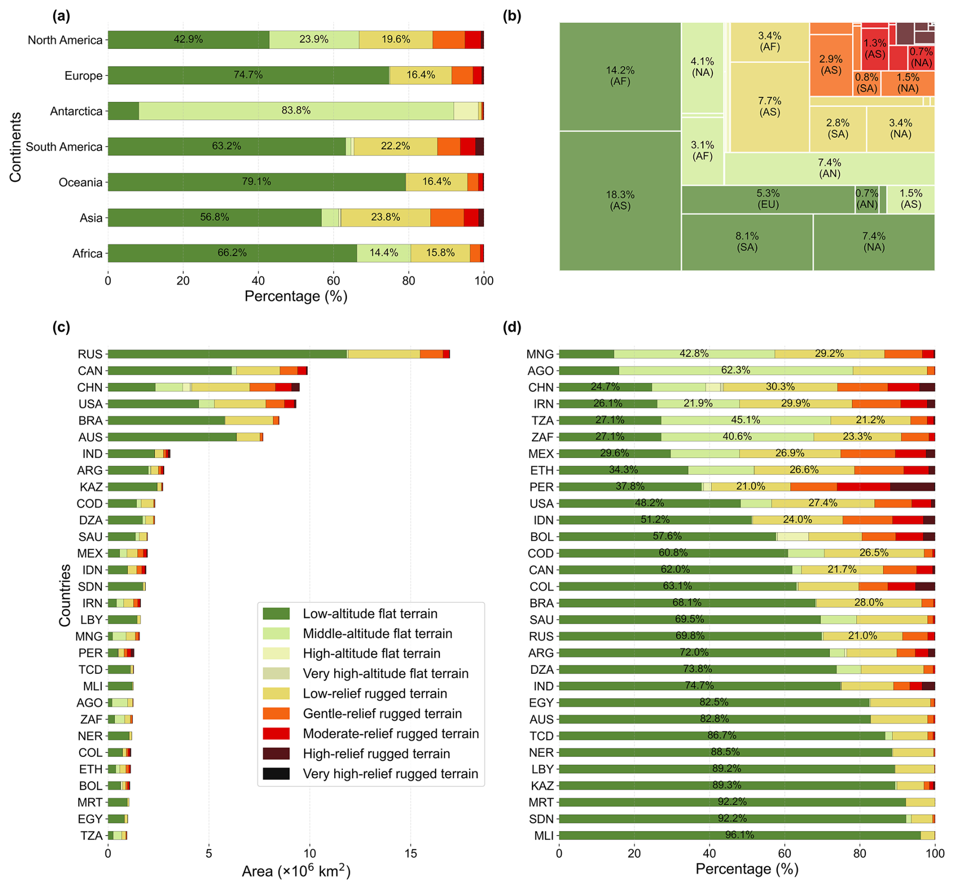
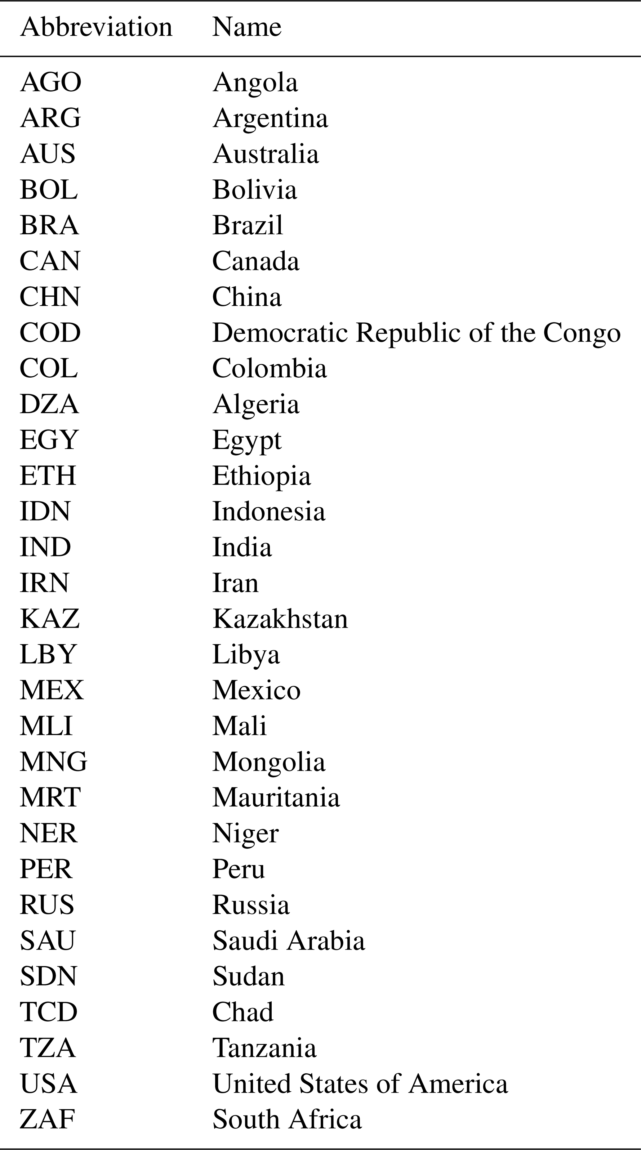
Figure 8 Area and proportional area statistics at the continental and national scales. (a) Proportion of GRC classes on each continent. (b) The square represents the proportion of each continent's relief types relative to the total global land area. A larger square indicates a greater area of that relief type for the continent. (c) Area of GRC classes in the top 30 countries ranked by area. (d) Proportion of GRC classes in the top 30 countries ranked by low-altitude flat terrain. Full names of the countries listed can be found in Table A2.

3.4 Geographic relationships: runoff, climate, and land use

In this section, we highlight the results of experiments performed to analyse the relationships between relief classes, surface runoff, climate, and land cover to highlight the potential applications of GRC. Based on the high-resolution results provided by GRC, we can explore the complex and in-depth relationships between various factors. Runoff data used in this study were obtained from GCN250 (Sujud and Jaafar, 2022), a global mean monthly runoff dataset for April 2015–2021 available in GeoTIFF format at 250 m resolution. This high-resolution dataset is valuable for a wide range of water-related applications, such as hydrological design, land management, water resource allocation, and flood risk assessment. As shown in Fig. 9 and marked by the red circles, we found that the spatial distribution of runoff closely aligns with the patterns represented by the GRC dataset. Notably, as shown in Fig. 9e to l, substantial differences in runoff values are observed at the boundaries between flat and rugged terrain, suggesting a strong association between runoff and terrain relief. This phenomenon indicates that the GRC data can help reveal such underlying spatial relationships. Moreover, in mountainous areas, the runoff values tend to follow valley-aligned patterns, which correspond well to the L2 classes in the GRC dataset. However, due to the coarse resolution of GCN250, these gradual transitions are not fully captured. As a detailed representation of terrain relief, the GRC dataset holds potential for supporting downscaling of global runoff data. Integrating both datasets offers novel insights into surface water dynamics and improves our understanding of water resource management under complex topographic conditions.

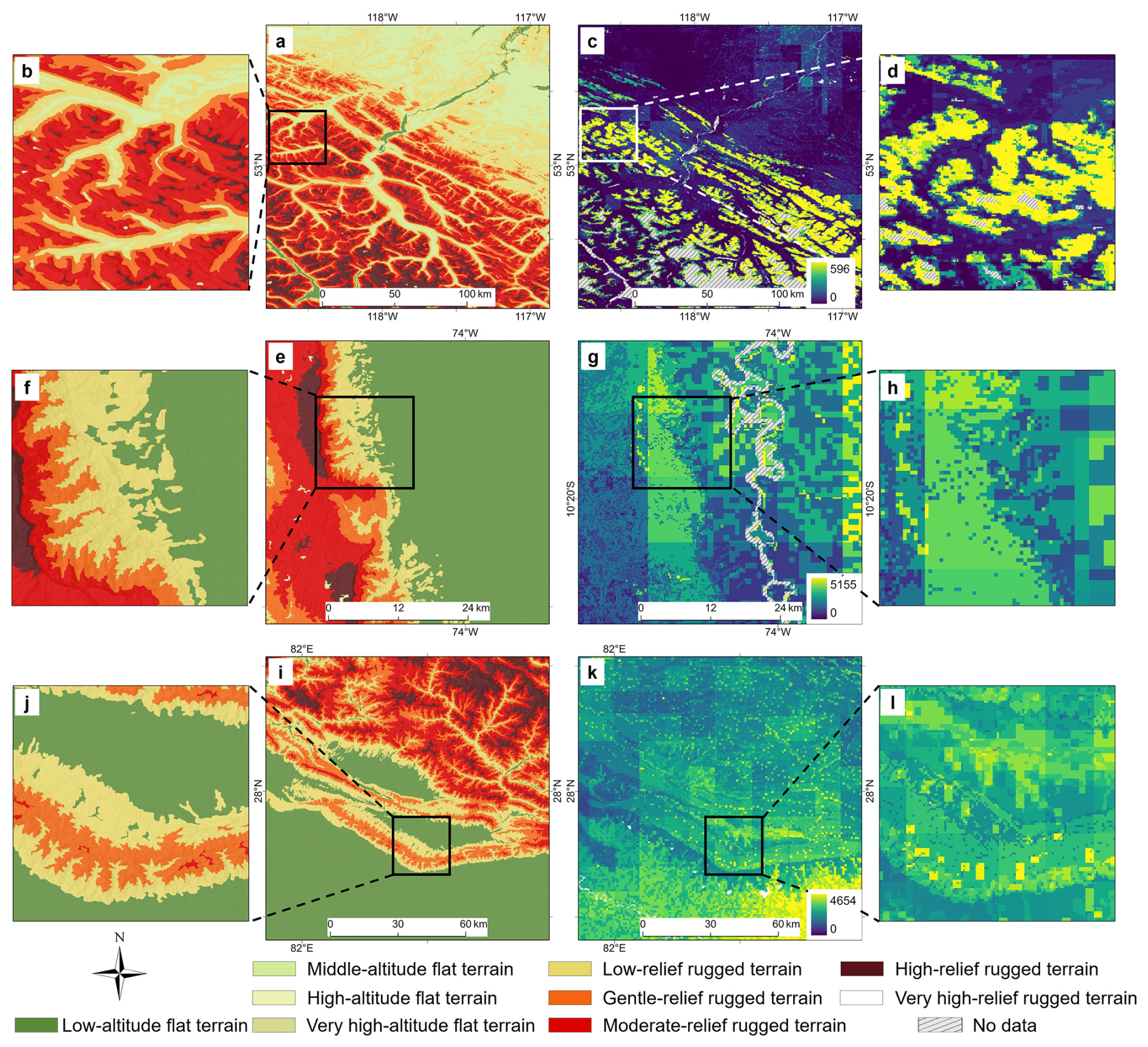
Figure 9 The spatial distribution of GRC and surface runoff in different areas. Panels (a) and (b) show the GRC L2 for the Rocky Mountains in North America, while panels (c) and (d) display the corresponding runoff patterns in the same region. Panels (e) and (f) show the GRC L2 for the Andes Mountains in South America, while panels (g) and (h) display the corresponding runoff patterns in the same region. Panels (i) and (j) show the GRC L2 and runoff in the southern areas of the Himalaya, while panels (k) and (l) display the corresponding runoff patterns in the same region.

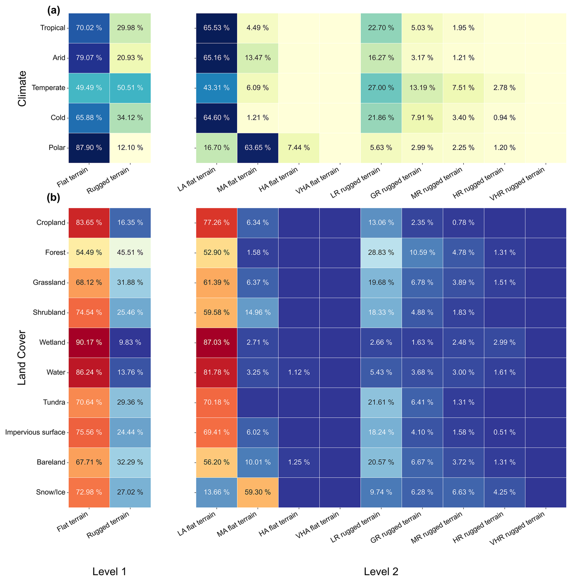
Figure 10 Relationship of relief classes with climate and land cover. Panels (a) and (b) show the proportions of the relief class in different climatic and land cover regions, respectively. Values less than 0.2 % are not labelled with numbers. Climate classes are as per the 1 km Köppen–Geiger climate classification maps for 1991–2020 (Beck et al., 2023). Land cover data are from FROM-GLC 30 m in 2017 (Yu et al., 2013). LA, MA, HA, and VHA represent low altitude, middle altitude, high altitude, and very high altitude, respectively. LR, GR, MR, HR, and VHR represent low relief, gentle relief, moderate relief, high relief, and very high relief, respectively.

As shown in Fig. 10, relief class distribution in temperate zones suggests a unique blend of climatic conditions and land surface processes, fostering a diverse array of relief classes. In the climatic zones of tropical, arid, and cold regions, we observe that low-altitude flat terrain and low-relief rugged terrain are most prominent. A special case occurs in the polar regions, where a large share of the surface area is situated at higher altitudes compared to other climate zones. This pattern is primarily attributed to the extensive occurrence of ice sheets, which substantially raise surface elevation and modify the observed relief patterns in these regions. Regarding land cover analysis (excluding the South Pole area), cropland occupies 83.65 % of flat terrain and 16.35 % of rugged terrain, yielding useful insights for analysing cultivated land productivity. Meanwhile, forests and bare land are more prevalent in moderately to highly rugged terrain, especially in low-relief areas. Additionally, the percentage of many ecologically significant biomes, such as forests, grasslands, wetlands, tundra, and water bodies, in flat and rugged regions has been brought up to date. This is potentially valuable for assessing the quality of ecosystems and carbon stocks.

GRC provided in this work has obvious applications in geomorphology but also in other fields and can, moreover, play a fundamental role in supporting the identification of landforms that incorporate domain background. For example, identification of a landscape element as “tableland” is complex, differs between disciplines, and requires that both morphological and evolutionary characteristics be accounted for. GRC can be integrated with additional observations to map the occurrence and distribution of tablelands through the delineation of segments that are elevated, flat, and surrounded by steep escarpments. There is also significant potential for the application of GRC to other fields (such as geology, hydrology, and ecology) focusing on the natural environment. For example, for ecologists, biodiversity distribution across different landform regions is one of the most significant issues and central to understanding the nature of ecosystem change. At the regional scale, contrasting geomorphological conditions are known to promote isolation of biological populations, influencing community structure and function as well as evolution. Meanwhile, the interaction between geomorphology and biogeography may result in complex bio-geomorphological dynamics. The feedback between physical, ecological, and evolutionary components constituting bio-geomorphological systems is an important element of the evolution of Earth's surface.

4 Code and data availability

The GRC V1.0 data are stored on the Deep-time Digital Earth Geomorphology platform and Zenodo (https://doi.org/10.5281/zenodo.15641257, Yang et al., 2024). We employed a 1° × 1° grid to tile the data for storage, with 25 252 file tiles in all. We distinguish the types of landform units by the coding attributes of the elements. Additionally, we provide a rasterized dataset (at 30 m resolution) using the coordinate system of WGS84 Web Mercator. Values of the cells represent the codes of L2 types. Meanwhile, in order to further the application, we also stored data in Esri shapefile format using the WGS84 coordinate system. The attribute table's field “code 1” is the landform type code of the first level (L1), and field “code 2” is the landform type code of sub-level L2. The core code used to produce this dataset is stored on Zenodo at https://doi.org/10.5281/zenodo.16979975 (Chen and Digital Terrain Analysis Group, 2025).

5 Conclusions

This study provides a novel global relief classification dataset with a resolution of 1 arcsec (approximately 30 m). In this study, we propose a framework for global land surface mapping to significantly improve the quantitative evaluation of topographic features. The key output is the release of the GRC dataset that is suited to applications across multiple disciplines, including geography, geology, ecology, and hydrology. Global-scale analysis of attributes within GRC reveals the composition and distribution of global landforms that enable comparison between regions and continents. The results emphasize the notable heterogeneity of Asia in general, and of China in particular, in terms of relief diversity. GRC outperforms previous datasets in expressing object details, providing an opportunity to investigate Earth's natural resources. The resolution of GRC is similar to that of the current mainstream remote sensing data, which makes combined use of the data relatively simple. We believe that this dataset can provide abundant and detailed geomorphological information for the field of Earth sciences, facilitating further advancements in related research.

Appendix A

Table A1 Classification of the global relief.

Table A2 Countries' names and their abbreviations.