the Creative Commons Attribution 4.0 License.
the Creative Commons Attribution 4.0 License.
 | 05 Feb 2025
A sea ice deformation and rotation rate dataset (2017–2023) from the Environment and Climate Change Canada automated sea ice tracking system (ECCC-ASITS)
Jean-François Lemieux
L. Bruno Tremblay
Amélie Bouchat
Damien Ringeisen
Philippe Blain
Stephen Howell
Mike Brady
Alexander S. Komarov
Béatrice Duval
Lekima Yakuden
Frédérique Labelle
Sea ice forms a thin but horizontally extensive boundary between the ocean and the atmosphere and has complex, crust-like dynamics characterized by intermittent sea ice deformations. The heterogeneity and localization of these sea ice deformations are important characteristics of the sea ice cover that can be used to evaluate the performance of dynamical sea ice models against observations across multiple spatial and temporal scales. Here, we present a new pan-Arctic sea ice deformation and rotation rate (SIDRR; https://doi.org/10.5281/zenodo.13936609, Plante et al., 2024a) dataset derived from the RADARSAT Constellation Mission (RCM) and Sentinel-1 (S1) synthetic aperture radar (SAR) imagery from 1 September 2017 to 31 August 2023. The SIDRR estimates are derived from contour integrals of triangulated ice motion data, obtained from the Environment and Climate Change Canada automated sea ice tracking system (ECCC-ASITS). The SIDRR dataset is not regularized and consists of stacked data from multiple SAR images computed on a range of spatial (4–10 km) and temporal (0.5–6 d) scales. It covers the entire Arctic Ocean and all peripheral seas except the Okhotsk Sea. Uncertainties associated with the propagation of tracking errors on the deformation values are included. We show that rectangular patterns of deformation features are visible when the sampled deformation rates are lower than the propagation error. This limits the meaningful information that can be extracted in areas with low SIDRR values but allows for the study of linear kinematic features with a high SIDRR signal-to-noise ratio. The spatial coverage and range of resolutions of the SIDRR dataset provide an interesting opportunity to investigate regional and seasonal variability in sea ice deformation statistics across scales, and these data can also be used to determine metrics for model evaluation.
- Article
(5067 KB) - Full-text XML
- BibTeX
- EndNote


As the perennial Arctic sea ice is declining, an increasing number of vessels are seasonally seen navigating the polar routes (Pizzolato et al., 2014, 2016; Dawson et al., 2018). However, navigation in ice-infested waters remains hazardous, leaving vessels with limited or no ice-breaking capability vulnerable to changing sea ice conditions (Mudryk et al., 2021; Chen et al., 2022). In particular, any changes to the sea ice drift may result in rapidly building sea ice pressure and far-reaching material deformations, such as fracturing, ridging and lead opening. The type, timing and location of these sea ice deformations can either ease or impede navigation and safety operations, but these factors remain difficult to predict due to the complex dynamics of sea ice as a thin layer of solid material subjected to large-scale surface forces (e.g., winds, tides and ocean currents). This difficulty can, in large part, be attributed to the multiscale character of this dynamics (Kwok, 2001; Lindsay and Stern, 2003; Marsan et al., 2004; Rampal et al., 2019) in a region with scarce observations, complicating model development and validation (Bouchat et al., 2022; Hutter et al., 2022).
Observations of sea ice deformation need to be derived from arrays of motion vectors, measured either in situ from drifting buoys (Heil et al., 1998; Hutchings et al., 2011, 2012; Itkin et al., 2017; Lei et al., 2020; Womack et al., 2024) or remotely by applying feature recognition and tracking methods on satellite imagery (Kwok, 2001; Komarov and Barber, 2014; Linow and Dierking, 2017; Korosov and Rampal, 2017; von Albedyll et al., 2024) or ship radar (Oikkonen et al., 2017). On the one hand, in situ observations have the advantage of producing high-precision data with frequent temporal sampling, but their point-data character usually makes for limited spatial coverage. On the other hand, remote-sensing observations gather a large number of data with multiscale information and coverage, but these observations yield lower-precision data and limited-temporal-resolution sampling. An advantage of the remote-sensing approaches is that they can be used to produce pan-Arctic sea ice motion fields (Lavergne et al., 2010; Tschudi et al., 2020; Tian et al., 2022; Lavergne and Down, 2023) and, thus, define sea ice motion seasonality, interannual variability and climatological trends. Gridded sea ice motion products, however, tend to involve filtering and post-processing methods that are not designed nor appropriate for computing sea ice deformations. For this reason, remote-sensing-derived sea ice deformations are usually produced independently of gridded sea ice motion products (e.g., Kwok, 2001; Bouillon and Rampal, 2015; von Albedyll et al., 2021).
In particular, the RADARSAT Geophysical Processor System (RGPS) (Kwok et al., 1998) was purposefully designed for the study of sea ice dynamics and was seminal for the establishment of large (Kwok et al., 2008) and multiscale (Marsan et al., 2004) sea ice deformation properties. The RGPS dataset corresponds to a list of Lagrangian tracks in the central Arctic produced by applying feature-tracking methods to synthetic aperture radar (SAR) imagery (Kwok et al., 1998). Each winter from 1997 to 2008, multi-month trajectories were initialized from SAR features organized on a regular 10 km resolution grid and then tracked for many months until spring (Kwok et al., 1998; Kwok and Cunningham, 2002). These trajectories were then used to derive the RGPS sea ice deformations (Kwok, 2001), from which a number of multiscale properties of sea ice dynamics were established, such as the power law of its observed probability distribution function (PDF) and spatiotemporal scaling properties (Bouchat and Tremblay, 2017; Rampal et al., 2019; Bouchat and Tremblay, 2020; Hutter and Losch, 2020). These diagnostics are the main source of validation for rheological models (e.g., in Ólason et al., 2022; Bouchat et al., 2022; Hutter et al., 2022), and the RGPS dataset currently remains the most common sea ice deformation reference for model development and validation (e.g., Bouchat and Tremblay, 2017; Spreen et al., 2017; Rampal et al., 2019; Hutter et al., 2018; Ringeisen et al., 2023). However, the widening gap between this reference period and the current state of the sea ice cover complicates the validation of sea ice dynamics in forecast systems, requiring hindcast simulations that are increasingly different from their operational framework.
In recent years, our ability to observe pan-Arctic sea ice motion has been improved by the deployment of several satellites equipped with SAR and with high pass frequency in the Arctic: the Sentinel-1 mission (S1, two satellites) and the RADARSAT Constellation Mission (RCM, three satellites). Sophisticated SAR feature-tracking algorithms have also been developed to efficiently process large numbers of SAR images (Komarov and Barber, 2014; Howell et al., 2022) and study regional sea ice dynamics (Babb et al., 2021; Moore et al., 2021). Together, this has paved the way for the development of the first operational sea ice motion product at Environment and Climate Change Canada (ECCC), based on an automated sea ice tracking system (ASITS; Howell et al., 2022). Designed to optimize the number of images processed to cover the entire Arctic, the ECCC-ASITS determines the sea ice motion at a 25 and 6.25 km resolution from S1 or RCM SAR image pairs. The ECCC RCM/S1 sea ice motion product is available from 2020 to present (Brady and Howell, 2021).
Here, we present a new pan-Arctic sea ice deformation and rotation rate (SIDRR) dataset based on S1 and RCM SAR imagery and derived from raw (non-gridded) ECCC-ASITS outputs. The SIDRR dataset covers the entire Arctic at variable spatiotemporal resolutions depending on the image acquisition and data processing, in the ranges of 2–10 km and 0.5–6 d. The data organization, its coverage and uncertainties are presented, and the limitations inherent to the use of the operational ASITS are discussed.
The paper is organized as follows: input data from the ECCC-ASITS used to produce the SIDRR dataset are described in Sect. 2; the production algorithm, SIDRR computation and associated uncertainties are presented in Sect. 3; characteristics of the dataset are detailed in Sect. 4, including the data format, the range of spatiotemporal scales and coverage; a discussion on data validation and uncertainties is provided in Sect. 5; and, finally, the conclusions are summarized in Sect. 7.
The ECCC-ASITS was developed to routinely generate pan-Arctic sea ice motion fields by processing an optimized number of SAR images to cover the entire Arctic within a limited time frame. The SAR images are taken from the S1 and RCM satellites, with images from each mission processed independently in different algorithm streams. The S1 mission includes two satellites (S1A and S1B) launched in 2014; of these satellites, S1A is still operational, whereas S1B stopped transmitting data in March 2021. The RCM includes three satellites launched in June 2019. The SIDRR dataset S1 stream, thus, covers the entire processed period (2017–2023), whereas the RCM stream is added from 29 January 2020 onward. Before the loss of S1B in December 2021, S1 had a slightly higher pass frequency in the central Arctic, but the RCM had a better coverage of the Canadian Arctic (see Howell et al., 2022, for more details). After 2021, the three-satellite RCM has much better coverage than S1A alone. Currently, RCM provides excellent daily or sub-daily coverage over the Canadian Arctic, whereas it offers coverage about once every 3 d over the Eurasian part of the Arctic. The original resolution of the S1 and RCM images depend on the beam mode, but all images are resampled to 200 m prior to running the ASITS.
The ECCC-ASITS proceeds as follows. First, the Arctic is divided into 400 km × 400 km sectors that are used to optimize the number of SAR images necessary to cover the entire Arctic. For each sector, a stack of images is created by selecting images that have at least a ∼30 % area overlap with the sector. The images within that stack are then paired if their area overlaps by at least 32 000 km2. Each initial image is only paired once – with the first match satisfying these criteria – before being removed from the stack. The algorithm of Komarov and Barber (2014) is applied to each selected pair to generate the sea ice motion (SIM) vectors, using a tracking resolution of 200 m and tracked-feature spacing of ∼8 km. The results from each pair of SAR images are output in a text file that lists all identified tracked features with their start location and displacement in X–Y pixel coordinates, latitudes, longitudes, and a measure of the confidence level in the feature tracking. Here, these ASITS sea ice motion vector outputs are used directly to generate the new sea ice deformation product, preserving their Lagrangian character (i.e., we do not use the ECCC-ASITS SIM gridded datasets, which are produced by aggregating and post-processing the SIM vectors).
A Python algorithm was developed to read the raw ECCC-ASITS output files, compute the sea ice deformations and uncertainties, and stack results in daily NetCDF output files. As in the ECCC-ASITS, each image pair is processed individually, organizing its tracked-feature start locations into a list of triangular arrays using Delaunay triangulation (Fig. 1). Triangles that are too thin (with angles <10°) or too big (area A>400 km2) are discarded. The sea ice drift, motion and deformations are computed for each triangle based on the end location of the tracked vertexes (Fig. 1c). Note that, as the SIDRR data are computed from the tracked-feature locations, they differ from results computed from the post-processed RCM/S1 sea ice motion product.
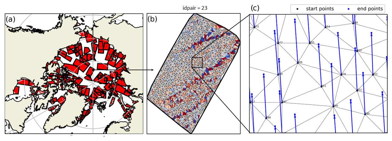
Figure 1Organization of the dataset: (a) tracked features (red) in the “SIDRR_20210212.nc” file, from the stacked SAR image pairs (black contours); (b) sea ice divergence calculated on the triangulated array from idpair = 23; and (c) a zoomed-in view of the triangular arrays from idpair = 23, showing the start positions (black dots), drift (blue arrows) and the end position (blue dots) of the tracked features. The vertex ID numbers are indicated in black.
3.1 Sea ice deformation computation
For each triangle, the sea ice deformation is computed using a line integral method (Bouchat and Tremblay, 2020; Bouchat et al., 2022) based on the velocity and start location of the tracked feature at each vertex. The area (A) of the triangle in the first image is first defined as follows:
where t represents the time level (acquisition time) of the first image, N is the number of vertexes in the array (here 3), and x and y indicate the position of vertex i (i increasing counterclockwise, using ) on the respective x and y axes. The sea ice motion components at each vertex are defined as follows:
where u and v represent the motion of the tracked features in the x and y direction, respectively, and Δt indicates the acquisition time difference between the paired images.
The strain rates are then given by the following:
where the x and y subscripts represent derivatives in the x and y directions, respectively.
The normal deformation rates (), shear deformation rates () and vorticity () are written as follows:
The total deformation rates are finally obtained from the strain rate invariants as follows:
To provide an example, the divergence deformation rates, shear deformation rates and rotation rates on 12 February 2021 are presented in Fig. 2. The computed sea ice deformation values are in the range of −1.0 to 1.0 d−1 for divergence and rotation and in the range of 0.0 to 1.0 d−1 for shear. The SIDRR data capture well the organization of the sea ice dynamics into localized lines of large deformation (known as linear kinematic features, or LKFs) and low deformation elsewhere. Large deformations are also seen in the marginal ice zone, where the rheology plays a lesser role due to the fragmented state of sea ice.
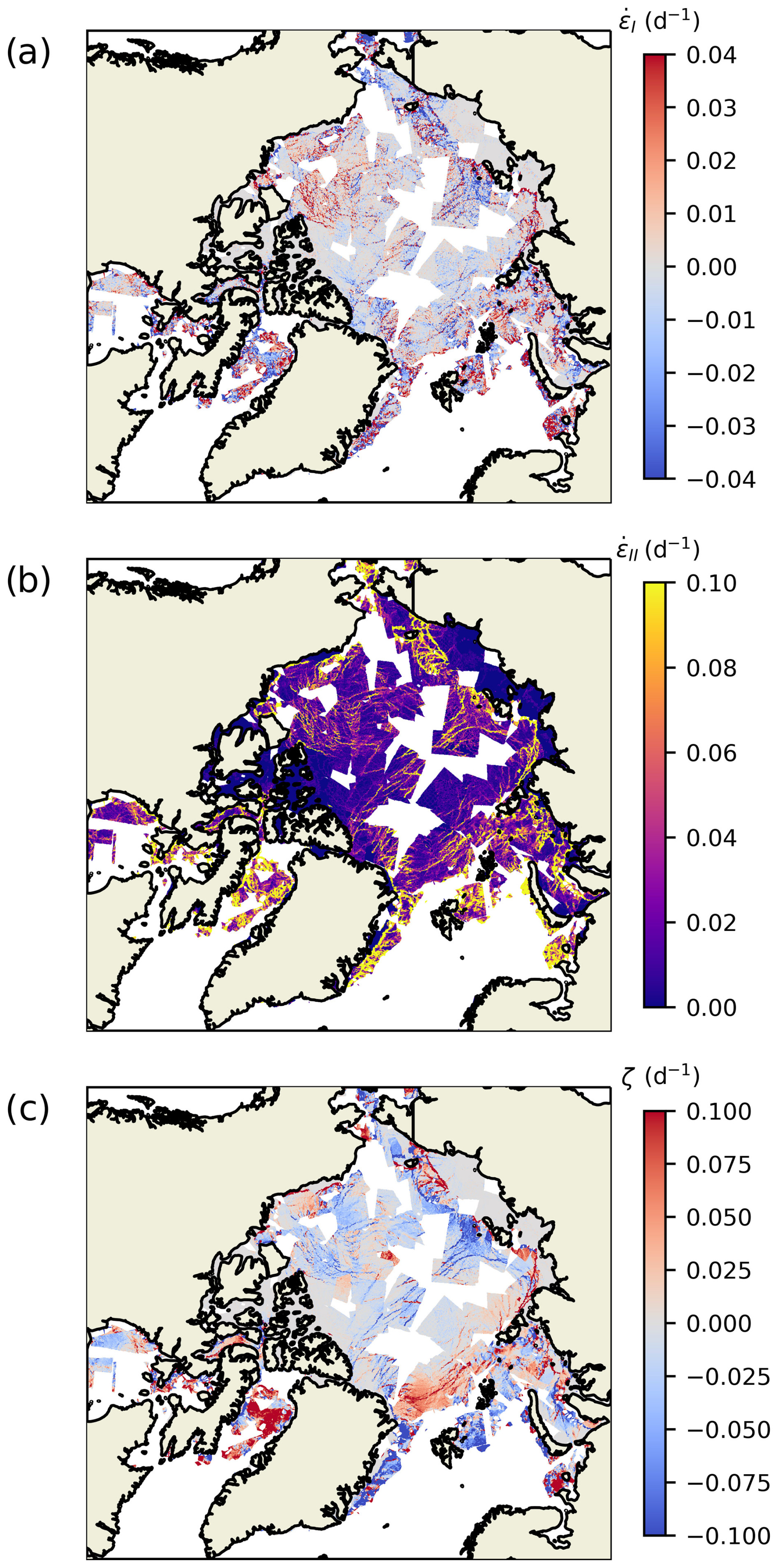
Figure 2Example of sea ice divergence (a), shear (b) and vorticity (c) on 12 February 2021.
3.2 Tracking uncertainty
The computed sea ice deformations have uncertainties associated with the tracking errors (propagation error) and with the small number of points (3) used to perform the contour integrals (boundary errors). These errors represent important limitations and need to be taken into account when producing sea ice deformation characteristics. While the boundary errors are difficult to quantify and need to be treated as part of post-processing by the users (Lindsay and Stern, 2003; Bouillon and Rampal, 2015; Griebel and Dierking, 2018), the propagation error is defined using propagation of uncertainties principles (Hutchings et al., 2011; Bouchat and Tremblay, 2020; Dierking et al., 2020). As such, in the SIDRR dataset, each computed sea ice deformation is assigned to a signal-to-noise value that can be used to filter the data according to the propagation error.
Assuming a positional error σx, the propagated error on the computed area (σA) and velocity (σu) are obtained from the following:
The propagated error on the computed deformation components is then expressed as follows (here showing only one component and neglecting the geolocation error; see Bouchat and Tremblay, 2020, for more details):
where represents the error on ux. The errors on the strain rate invariants and rotation rates are expressed in terms of the errors on each component, as follows:
The error on the total deformation rate is expressed as follows:
The signal-to-noise ratio (s) is then defined as the relative magnitude of the total deformation rates with respect to the total deformation error:
4.1 Format
The SIDRR data are stored in daily NetCDF files using a “SIDRR_YYYYMMDD.nc” nomenclature. Each file contains the data from all paired SAR images with an initial (first image) acquisition time within the given date. The recorded variables are listed in Table 1 and have the shape of vectors of length “n” (corresponding to the total number of triangles stacked in the NetCDF files) or “npts” (the number of triangulated tracked features). The dataset includes all of the necessary information to visualize or post-process the SIDRR data. ID numbers are also provided to identify each SAR image pair (“idpairs”), triangle (“n”) and tracked feature (“ids1”,“ids2” and “ids3”; one for each vertex). The tracked-feature IDs are attributed independently (i.e., they recur) for each image pair.
Table 1Description of dataset variables and dimensions.
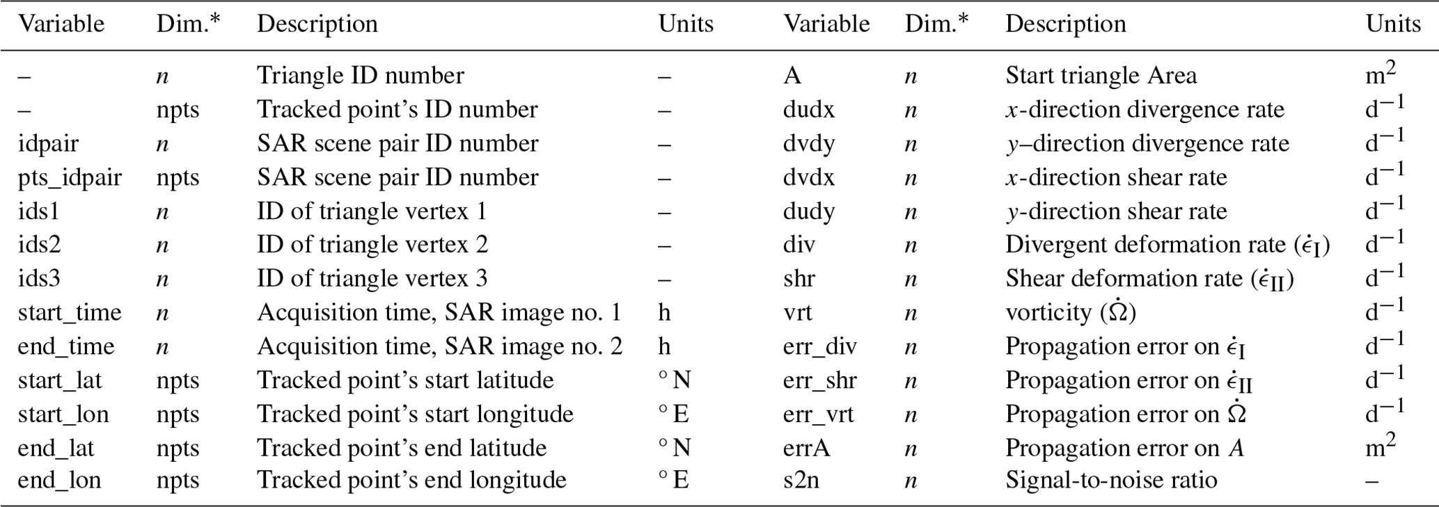
* “Dim.” denotes dimension.
The SIDRR data have not been regularized and correspond to a patchwork of data from different SAR scenes computed over a range of spatiotemporal scales (see Sect. 4.2). As such, there are large areas without data between the processed scenes or regions with overlaps (see, for instance, Fig. 1a). This differs from the RGPS dataset in which the tracked features are initially organized on a 10 km resolution rectilinear grid and then tracked for the entire winter, allowing for a nearly contiguous mapping of sea ice deformations in the central Arctic (Kwok et al., 2008; Bouchat and Tremblay, 2020). Here, the post-processing steps necessary to produce a contiguous (regularized) pan-Arctic mapping of sea ice deformations remain to be established; this is left for future work. This allows for the use of this SIDRR dataset to test different post-processing approaches and their impact on diagnostics used for model validation.
4.2 Spatiotemporal characteristics
4.2.1 Scale
The SIDRR data are computed from triangular arrays with variable sizes; the effective radius () of each triangle in the dataset is distributed around a mean of ∼6.7 km but ranges from a minimum of 2 km to a maximum of ∼15 km (Fig. 3a). This distribution is coherent with the target feature-spacing resolution in the ECCC-ASITS (∼8 km) and variations associated with the exact location (or absence) of identifiable SAR texture features. Note that the distributions are nearly identical for data computed from S1 and RCM images, which is unsurprising given that the images are processed using the same algorithm, although in different streams.
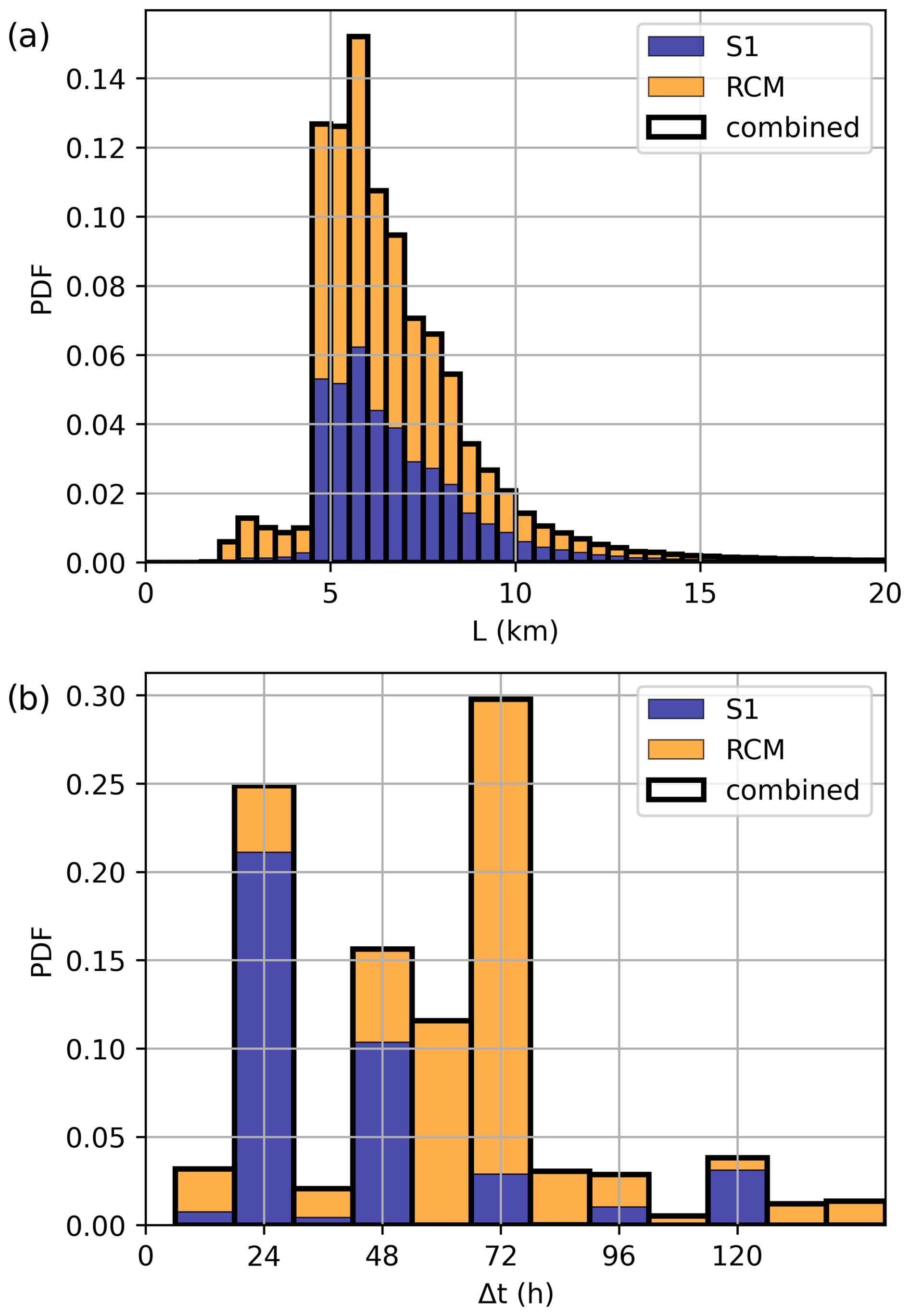
Figure 3Distribution of the spatial (a) and temporal (b) scales of the computed deformations, in the period with both S1 and RCM data (1 February 2020 to 31 August 2023). Colours indicate the contribution from data in the S1 and RCM streams.
The SIDRR data are also computed at different temporal scales (Fig. 3b), depending on the time difference between the acquisition of the paired SAR images. These time intervals depend on the method used in the ECCC-ASITS to pair the SAR images (Howell et al., 2022); this is made sequentially by selecting the first image satisfying some set of criteria (e.g., minimum time or minimum overlapping area). As the S1 and RCM images are processed in different streams, their temporal scale distributions present differences associated with their respective frequency of satellite passes. Most of the S1 image pairs present 24 h intervals, with many sub-daily and some at 48, 72 and 96 h intervals. The RCM image pairs mostly present 60 and 72 h intervals. These differences largely affect the magnitude of the computed sea ice deformations, and they need to be taken into account when producing pan-Arctic SIDRR statistics.
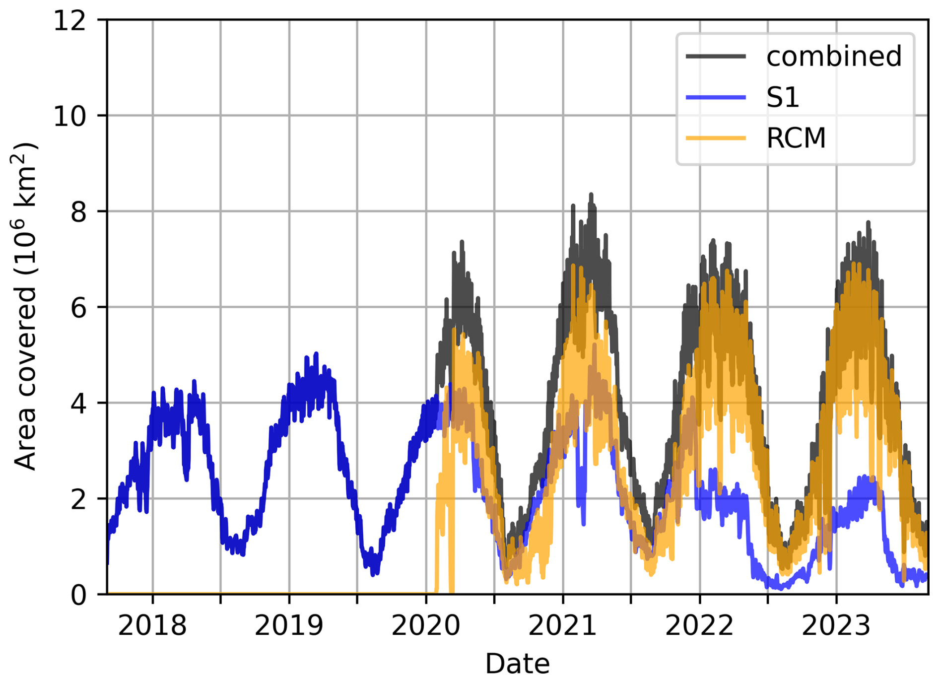
Figure 4Time series of the area with valid deformation data from 1 September 2017 to 31 August 2023, for the S1 data (blue), the RCM data (orange) and both combined (black).
4.2.2 Coverage
The total area covered daily in the SIDRR dataset has a strong seasonal cycle; this is partly due to the seasonality in the sea ice cover itself as well as to the difficult identification of SAR features in summer, which reduces the success rate of the tracking algorithm. The winter season (January to March) features a maximum coverage of km2 before 2020, climbing to km2 once RCM data are included. This is about ∼50 % of the pan-Arctic maximum sea ice extent (Fetterer et al., 2017). In summer (from July to September), the SIDRR dataset area coverage falls to km2 (about ∼20 % of the National Snow and Ice Data Center, NSIDC, minimum extent). Thus, including the RCM data nearly doubles the coverage of the dataset. Note that this represents a significant improvement compared with the RGPS coverage, which was limited to the central Arctic.
Despite the numerous gaps between SAR images in specific daily files, the percent daily coverage in winter is high (>50 %) over most of the Arctic Basin, nearing 100 % of days covered in some areas once the RCM data are added (from 2020 onward; see Fig. 5a–c). The local temporal sampling is nearly daily over the entire Arctic, including all peripheral seas except the Okhotsk Sea, which is not covered by the ASITS. This demonstrates the benefits of including the RCM images: while the coverage from S1 images is generally good in the high Arctic, the RCM data show a smaller North Pole blind spot and are more evenly distributed, raising the coverage in the peripheral seas. In summer, near-daily coverage is seen in the high Arctic (northward of 80° N), but this coverage is low elsewhere where marginal ice zone dynamics dominates (Fig. 5d–f).
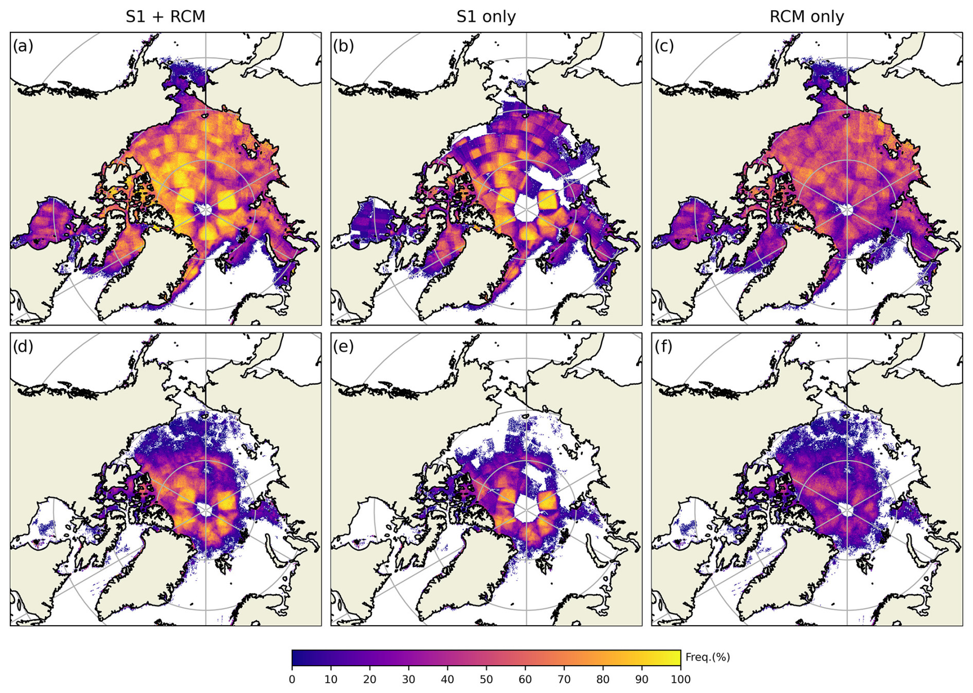
Figure 5Percent daily coverage from the SI/RCM sea ice deformation rate dataset in winter (from 1 January to 31 March) 2021 (a–c) and summer (1 July to 30 September) 2021 (d–f), using data from both the S1 and RCM streams (a, d), only the S1 stream (b, e), and only the RCM stream (c, f).
Note that the presence of square regions with higher coverage is associated with the ASITS method for optimizing the number of SAR scenes to cover the entire Arctic, leaving a tendency for gaps at the border of each selection areas (see Fig. 6 in Howell et al., 2022). Increasing the number of processed RCM images can reduce this uneven sampling effect, but this would need to be performed outside of the operational ASITS framework.
Validation of the SIDRR features is complicated by (1) the scale dependency of the computed sea ice deformation magnitude, making for difficult interpretation of side-by-side comparisons unless the products are computed on the exact same spatiotemporal scales; (2) the lack of independent sea ice motion products covering the same period at similar resolution; and (3) the yet unknown impact of post-processing methods (part of producing gridded sea ice motion products) on sea ice deformation values. These difficulties are common to any sea ice deformation products, and the SIDRR dataset is published in part to mitigate these difficulties by providing an independent yet flexible dataset that can be used by the sea ice dynamics community.
Nonetheless, the ECCC-ASITS sea ice motion data themselves have been thoroughly validated and have been shown to have good correspondence against other products (see Howell et al., 2022, for details). Here, we use the ECCC-ASITS sea ice motion uncertainties – as well as their propagation into SIDRR errors – as a form of validation and also discuss the limitations that they represent in terms of the resolved features. Further validation in the form of comparisons with other sea ice deformation measurements is planned for future work and will be conducted as part of in-depth investigations of the SIDRR characteristics (power law, spatiotemporal scaling and LKFs) and their sensitivity to post-processing methods.
The sea ice displacement data from ASITS have been shown to have a (pan-Arctic) root-mean-square error (RMSE) of 2.78 km and mean deviation (MD) of 0.40 km against buoys. These values are coherent with the tracking being performed at a pixel resolution (tracking error σx) of 200 m. Based on the propagation of this tracking error into the computed SIDRR values, the precision of the SIDRR data is in the range of ∼0–0.1 d−1 (Fig. 6a), depending on the spatiotemporal scale of the computation. Most of the sea ice deformations display small signal-to-noise values (s<1; Fig. 6b). The data computed from RCM images present lower errors due to the predominance of a longer (72 h) acquisition time difference. This uncertainty is quite large compared with other studies: in the RGPS data, the propagation of the tracking error into a computed area was estimated to be ∼1.4 % in the case of 100 km2 quadrangle cells, leading to a sea ice deformation uncertainty of 0.005 d−1 if computed over a 3 d period.
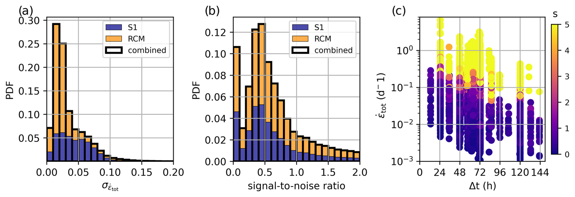
Figure 6Distribution (combining the S1 and RCM stream) of total deformation rate propagation errors (a), distribution of the data signal-to-noise ratio (b) and scatter of the total sea ice deformation rates (c) as function of the computation timescale (x axis) and the signal-to-noise ratio (in colour), in the period with both RCM and S1 data (1 February 2020 to 31 August 2023). Colours in the distributions (a, b) indicate the contribution from data from the S1 and RCM streams.
The larger SIDRR uncertainty in the present dataset is a consequence of making an opportunistic use of the ECCC-ASITS algorithm, which was designed to produce pan-Arctic sea ice motion maps within an operational time frame, balancing positional precision with computational costs. Specifically, compared with RGPS, our sea ice deformations have larger propagation error due to the following reasons: (1) the tracking resolution of 200 m in the ECCC-ASITS algorithm (vs. 100 m in RGPS), (2) smaller (often 24 h) timescales (vs. 3 d in RGPS) and (3) the computation of deformations over triangular arrays (vs. a rectangular grid in RGPS). It is likely that this uncertainty can be lowered by applying post-processing and data aggregation methods, although this would be at the cost of losing smaller-scale information. This will be explored in future work.
The analysis reveals that the SIDRR data are well split between highly uncertain values in low-deformation areas and meaningful values in high-deformation areas. In particular, low-deformation areas are prone to displaying rectangular artefact patterns where the nominal resolution of the feature tracking is not sufficient to capture the gradients in sea ice displacement (Fig. 7a and b). These artefacts appear when the drift distance presents step-like jumps corresponding to the tracking resolution (σx=200 m in our case; see Fig. 7c), concentrating an originally smooth deformation field into localized lines. The squared signal-to-noise values (s2) can be used as a proxy to differentiate these artefact from LKFs, with s2>1.0 for LKFs and s2<1.0 for artefacts (Fig. 7d).
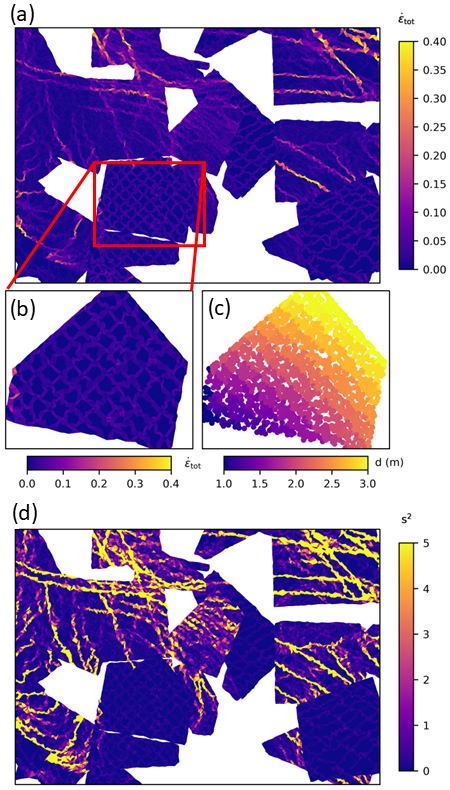
Figure 7Example of artefacts associated with the feature-tracking resolution not resolving gradients in sea ice displacement. Larger panels show the total sea ice deformation rates (a) and squared signal-to-noise ratio (d) from multiple SAR scenes in the central Arctic, close to the North Pole, on 6 March 2021. Small panels show a zoomed-in view of the total sea ice deformation rates in the SAR image pair with ID = 252 (b) with the associated poorly resolved (step-like) displacement field (c). The squared signal-to-noise ratio in panel (d) effectively differentiates the artefacts from the LKFs.
Note that the analysis above does not consider uncertainties associated with the approximation of SIDRR from triangular arrays. These boundary errors are not related to the tracking uncertainty but are likely as significant (Lindsay and Stern, 2003), as attested by the noisy appearance of the divergence rate fields in the resolved LKFs (see Fig. 1b). Different filtering approaches (e.g., Bouillon and Rampal, 2015; Griebel and Dierking, 2018) can (and must) be used by the user as part of post-processing of the SIDRR dataset, and these techniques will be explored in future work.
The SIDRR dataset is available from https://doi.org/10.5281/zenodo.13936609 (Plante et al., 2024a). The Python code used to produce the SIDRR dataset is available at https://doi.org/10.5281/zenodo.14783107 (Plante et al., 2025). The Python scripts used for the data analysis and the figures are available at https://doi.org/10.5281/zenodo.13936712 (Plante et al., 2024b).
A sea ice deformation and rotation rate (SIDRR) dataset is constructed based on the sea ice motion vectors obtained from the Environment and Climate Change Canada automated sea ice tracking system (ECCC-ASITS; Howell et al., 2022). Developed for operational purposes, the ECCC-ASITS retrieves the sea ice drift from conjoined SAR images by applying the feature-tracking algorithm of Komarov and Barber (2014) to S1 and RCM data. The SIDRR data are computed using a line integral approach based on the triangulated start (and end) location of the ECCC-ASITS tracked features.
The SIDRR dataset is organized into daily NetCDF files, with each stacking the SIDRR information from all of the conjoined SAR images with an initial acquisition time within the given date. To preserve data flexibility, the dataset is kept as “raw” as possible and remains highly irregular, with each file containing a patchwork SIDRR data from multiple SAR images. The SIDRR data are defined from ranges of temporal (0.5 to 6 d) and spatial (∼2.0 to ∼10.0 km) scales. Different post-processing methods will be tested in future work to determine their influence on the spatiotemporal scaling properties and other metrics commonly used for sea ice modelling and forecasting applications.
The SIDRR dataset (2017–2023) offers yearlong, pan-Arctic (except the Okhotsk Sea) coverage at least at a weekly frequency, with a significant portion of the data presenting daily coverage. The inclusion of summer months and the marginal seas is a significant improvement from the commonly used RGPS dataset (Kwok et al., 1998). The inclusion of RCM data from January 2020 onward significantly improves the spatiotemporal coverage, reaching ∼50 % and 20 % of the sea ice cover in winter and summer, respectively. This extensive coverage represents an asset to investigate differences in sea ice dynamics between the recent (2017–2023) and RGPS (1997–2008) periods, to establish pan-Arctic and regional SIDRR spatiotemporal characteristics and study their seasonality.
The SIDRR dataset is shown to resolve localized zones of large deformations (or linear kinematic features, LKFs) between areas of uncertain and low deformations. However, the relatively low feature-tracking resolution (200 m) yields large uncertainties in SIDRR (significantly larger than in the RGPS dataset). These uncertainties are shown to cause localized artefacts similar to LKFs. Signal-to-noise values are proven to be efficient in differentiating the certain high-deformation features in LKFs from these tracking error artefacts. The extent to which these errors (along with boundary errors) can be reduced via post-processing methods will be assessed in future work.
Many of the constraints in the current analysis come from ECCC-ASITS being designed for operational purposes, with a need for computational efficiency. Note that, despite these constraints, the operational character of the ECCC-ASITS remains beneficial, with its ongoing production making for likely yearly extensions of the present SIDRR dataset in the coming years. Nonetheless, the constraints result in much potential for future improvements to the dataset by (1) reducing the tracking errors, (2) increasing the resolution of the tracked features (increasing the SIDRR dataset resolution) and (3) increasing the number of processed SAR images. These improvements are currently under development and will allow for useful extensions of sea ice deformation observations from remote sensing towards the kilometre scale.
The ECCC-ASITS sea ice motion vector outputs were provided by MB, ASK and SH, along with technical support and guidance. BD and LY developed the Python code to process the ECCC-ASITS data and compute the sea ice deformations, with contributions from AB, PB, JFL, MP, DR and LBT. The data analysis and figures were coded and analyzed by MP, AB, DR, LY and BD. MP wrote the manuscript with contributions from AB, ASK, SH, JFL, DR and LBT.
The contact author has declared that none of the authors has any competing interests.
Publisher's note: Copernicus Publications remains neutral with regard to jurisdictional claims made in the text, published maps, institutional affiliations, or any other geographical representation in this paper. While Copernicus Publications makes every effort to include appropriate place names, the final responsibility lies with the authors.
The authors wish to thank the editor, Petra Heil; the reviewer, Anton Korosov; and the two other anonymous reviewers for their valuable comments that improved the quality of this paper.
This work is a contribution to a Canadian Space Agency (CAS) Research Opportunity in Space Science (ROSS-Cycle III; grant no. 23SUESDEFO awarded to L. Bruno Tremblay).
This paper was edited by Petra Heil and reviewed by Anton Korosov and two anonymous referees.
Babb, D. G., Kirillov, S., Galley, R. J., Straneo, F., Ehn, J. K., Howell, S. E. L., Brady, M., Ridenour, N. A., and Barber, D. G.: Sea ice dynamics in Hudson Strait and its impact on winter shipping operations, J. Geophys. Res.-Oceans, 126, e2021JC018024, https://doi.org/10.1029/2021JC018024, 2021. a
Bouchat, A. and Tremblay, B.: Using sea-ice deformation fields to constrain the mechanical strength parameters of geophysical sea ice, J. Geophys. Res.-Oceans, 122, 5802–5825, https://doi.org/10.1002/2017JC013020, 2017. a, b
Bouchat, A. and Tremblay, B.: Reassessing the quality of sea-ice deformation estimates derived from the RADARSAT geophysical processor system and its impact on the spatiotemporal scaling statistics, J. Geophys. Res.-Oceans, 125, e2019JC015944, https://doi.org/10.1029/2019JC015944, 2020. a, b, c, d, e
Bouchat, A., Hutter, N., Chanut, J., Dupont, F., Dukhovskoy, D., Garric, G., Lee, Y. J., Lemieux, J.-F., Lique, C., Losch, M., Maslowski, W., Myers, P. G., Ólason, E., Rampal, P., Rasmussen, T., Talandier, C., Tremblay, B., and Wang, Q.: Sea Ice Rheology Experiment (SIREx): 1. Scaling and statistical properties of sea-ice deformation fields, J. Geophys. Res.-Oceans, 127, e2021JC017667, https://doi.org/10.1029/2021JC017667, 2022. a, b, c
Bouillon, S. and Rampal, P.: On producing sea ice deformation data sets from SAR-derived sea ice motion, The Cryosphere, 9, 663–673, https://doi.org/10.5194/tc-9-663-2015, 2015. a, b, c
Brady, M. and Howell, S. E. L.: RADARSAT Constellation Mission / Sentinel-1 Sea Ice Motion (RCMS1SIM), https://catalogue.ec.gc.ca/geonetwork/srv/api/records/09ab22c4-e211-4d23-afe6-9e7aa6831c62 (last access: December 2024), 2021. a
Chen, J., Kang, S., You, Q., Zhang, Y., and Du, W.: Projected changes in sea ice and the navigability of the Arctic passages under global warming of 2 °C and 3 °C, Anthropocene, 40, 100349, https://doi.org/10.1016/j.ancene.2022.100349, 2022. a
Dawson, J., Pizzolato, L., Howell, S. E., Copland, L., and Johnston, M. E.: Temporal and spatial patterns of ship traffic in the Canadian Arctic from 1990 to 2015, Arctic, 71, 15–26, 2018. a
Dierking, W., Stern, H. L., and Hutchings, J. K.: Estimating statistical errors in retrievals of ice velocity and deformation parameters from satellite images and buoy arrays, The Cryosphere, 14, 2999–3016, https://doi.org/10.5194/tc-14-2999-2020, 2020. a
Fetterer, F., Knowles, K., Meier, W. N., Savoie, M., and Windnagel, A. K.: Sea Ice Index. (G02135, Version 3), Boulder, Colorado USA, National Snow and Ice Data Center [data set], https://doi.org/10.7265/N5K072F8, 2017. a
Griebel, J. and Dierking, W.: Impact of sea ice drift retrieval errors, discretization and grid type on calculations of ice deformation, Remote Sens.-Basel, 10, 393, https://doi.org/10.3390/rs10030393, 2018. a, b
Heil, P., Lytle, V. I., and Allison, I.: Enhanced thermodynamic ice growth by sea-ice deformation, Ann. Glaciol., 27, 433–437, https://doi.org/10.3189/1998AoG27-1-433-437, 1998. a
Howell, S. E. L., Brady, M., and Komarov, A. S.: Generating large-scale sea ice motion from Sentinel-1 and the RADARSAT Constellation Mission using the Environment and Climate Change Canada automated sea ice tracking system, The Cryosphere, 16, 1125–1139, https://doi.org/10.5194/tc-16-1125-2022, 2022. a, b, c, d, e, f, g
Hutchings, J. K., Roberts, A., Geiger, C. A., and Richter-Menge, J.: Spatial and temporal characterization of sea-ice deformation, Ann. Glaciol., 52, 360–368, https://doi.org/10.3189/172756411795931769, 2011. a, b
Hutchings, J. K., Heil, P., Steer, A., and Hibler III, W. D.: Subsynoptic scale spatial variability of sea ice deformation in the western Weddell Sea during early summer, J. Geophys. Res.-Oceans, 117, C01002, https://doi.org/10.1029/2011JC006961, 2012. a
Hutter, N. and Losch, M.: Feature-based comparison of sea ice deformation in lead-permitting sea ice simulations, The Cryosphere, 14, 93–113, https://doi.org/10.5194/tc-14-93-2020, 2020. a
Hutter, N., Losch, M., and Menemenlis, D.: Scaling properties of Arctic sea ice deformation in a high-resolution viscous-plastic sea ice model and in satellite observations, J. Geophys. Res.-Oceans, 123, 672–687, https://doi.org/10.1002/2017JC013119, 2018. a
Hutter, N., Bouchat, A., Dupont, F., Dukhovskoy, D., Koldunov, N., Lee, Y. J., Lemieux, J.-F., Lique, C., Losch, M., Maslowski, W., Myers, P. G., Ólason, E., Rampal, P., Rasmussen, T., Talandier, C., Tremblay, B., and Wang, Q.: Sea Ice Rheology Experiment (SIREx): 2. Evaluating linear kinematic features in high-resolution sea ice simulations, J. Geophys. Res.-Oceans, 127, e2021JC017666, https://doi.org/10.1029/2021JC017666, e2021JC017666 2021JC017666, 2022. a, b
Itkin, P., Spreen, G., Cheng, B., Doble, M., Girard-Ardhuin, F., Haapala, J., Hughes, N., Kaleschke, L., Nicolaus, M., and Wilkinson, J.: Thin ice and storms: Sea ice deformation from buoy arrays deployed during N-ICE2015, J. Geophys. Res.-Oceans, 122, 4661–4674, https://doi.org/10.1002/2016JC012403, 2017. a
Komarov, A. S. and Barber, D. G.: Sea ice motion tracking from sequential dual-polarization RADARSAT-2 Images, IEEE T. Geosci. Remote, 52, 121–136, https://doi.org/10.1109/TGRS.2012.2236845, 2014. a, b, c, d
Korosov, A. A. and Rampal, P.: A combination of feature tracking and pattern matching with optimal parametrization for sea ice drift retrieval from SAR data, Remote Sens.-Basel, 9, 258, https://doi.org/10.3390/rs9030258, 2017. a
Kwok, R.: Deformation of the Arctic Ocean Sea Kwok, R.: Deformation of the Arctic Ocean Sea Ice Cover between November 1996 and April 1997: A Qualitative Survey, in: IUTAM Symposium on Scaling Laws in Ice Mechanics and Ice Dynamics. Solid Mechanics and Its Applications, edited by: Dempsey, J. P. and Shen, H. H., vol. 94, Springer, Dordrecht, https://doi.org/10.1007/978-94-015-9735-7_26, 2001. a, b, c, d
Kwok, R. and Cunningham, G. F.: Seasonal ice area and volume production of the Arctic Ocean: November 1996 through April 1997, J. Geophys. Res.-Oceans, 107, SHE 12–1–SHE 12–17, https://doi.org/10.1029/2000JC000469, 2002. a
Kwok, R., Schweiger, A., Rothrock, D. A., Pang, S., and Kottmeier, C.: Sea ice motion from satellite passive microwave imagery assessed with ERS SAR and buoy motions, J. Geophys. Res.-Oceans, 103, 8191–8214, https://doi.org/10.1029/97JC03334, 1998. a, b, c, d
Kwok, R., Hunke, E. C., Maslowski, W., Menemenlis, D., and Zhang, J.: Variability of sea ice simulations assessed with RGPS kinematics, J. Geophys. Res.-Oceans, 113, C11012, https://doi.org/10.1029/2008JC004783, 2008. a, b
Lavergne, T. and Down, E.: A climate data record of year-round global sea-ice drift from the EUMETSAT Ocean and Sea Ice Satellite Application Facility (OSI SAF), Earth Syst. Sci. Data, 15, 5807–5834, https://doi.org/10.5194/essd-15-5807-2023, 2023. a
Lavergne, T., Eastwood, S., Teffah, Z., Schyberg, H., and Breivik, L.-A.: Sea ice motion from low-resolution satellite sensors: an alternative method and its validation in the Arctic, J. Geophys. Res.-Oceans, 115, C10032, https://doi.org/10.1029/2009JC005958, 2010. a
Lei, R., Gui, D., Hutchings, J. K., Heil, P., and Li, N.: Annual Cycles of Sea Ice Motion and Deformation Derived From Buoy Measurements in the Western Arctic Ocean Over Two Ice Seasons, J. Geophys. Res.-Oceans, 125, e2019JC015310, https://doi.org/10.1029/2019JC015310, 2020. a
Lindsay, R. W. and Stern, H. L.: The RADARSAT geophysical processor system: quality of sea ice trajectory and deformation estimates, J. Atmos. Ocean. Tech., 20, 1333–1347, https://doi.org/10.1175/1520-0426(2003)020<1333:TRGPSQ>2.0.CO;2, 2003. a, b, c
Linow, S. and Dierking, W.: Object-based detection of linear kinematic features in sea ice, Remote Sens.-Basel, 9, 493, https://doi.org/10.3390/rs9050493, 2017. a
Marsan, D., Stern, H., Lindsay, R., and Weiss, J.: Scale dependence and localization of the deformation of Arctic Sea Ice, Phys. Rev. Lett., 93, 178501, https://doi.org/10.1103/PhysRevLett.93.178501, 2004. a, b
Moore, G. W. K., Howell, S. E. L., Brady, M., Xu, X., and McNeil, K.: Anomalous collapses of Nares Strait ice arches leads to enhanced export of Arctic sea ice, Nat. Commun., 12, 1, https://doi.org/10.1038/s41467-020-20314-w, 2021. a
Mudryk, L. R., Dawson, J., Howell, S. E. L., Derksen, C., Zagon, T. A., and Brady, M.: Impact of 1, 2 and 4 °C of global warming on ship navigation in the Canadian Arctic, Nat. Clim. Change, 11, 673–679, https://doi.org/10.1038/s41558-020-0757-5, 2021. a
Oikkonen, A., Haapala, J., Lensu, M., Karvonen, J., and Itkin, P.: Small-scale sea ice deformation during N-ICE2015: from compact pack ice to marginal ice zone, J. Geophys. Res.-Oceans, 122, 5105–5120, https://doi.org/10.1002/2016JC012387, 2017. a
Ólason, E., Boutin, G., Korosov, A., Rampal, P., Williams, T., Kimmritz, M., Dansereau, V., and Samaké, A.: A new brittle rheology and numerical framework for large-scale sea-ice models, J. Adv. Model. Earth Sy., 14, e2021MS002685, https://doi.org/10.1029/2021MS002685, 2022. a
Pizzolato, L., Howell, S. E. L., Derksen, C., Dawson, J., and Copland, L.: Changing sea ice conditions and marine transportation activity in Canadian Arctic waters between 1990 and 2012, Climatic Change, 123, 161–173, https://doi.org/10.1007/s10584-013-1038-3, 2014. a
Pizzolato, L., Howell, S. E. L., Dawson, J., Laliberté, F., and Copland, L.: The influence of declining sea ice on shipping activity in the Canadian Arctic, Geophys. Res. Lett., 43, 12146–12154, https://doi.org/10.1002/2016GL071489, 2016. a
Plante, M., Lemieux, J.-F., Tremblay, L. B., Bouchat, A., Ringeisen, D., Blain, P., Howell, S., Brady, M., Alexander, K., Duval, B., Yakuden, L., and Labelle, F.: Sea ice deformation and rotation rates (SIDRR) from the ECCC-ASITS, Zenodo [data set], https://doi.org/10.5281/zenodo.13936609, 2024a. a, b
Plante, M., Yakuden, L., Duval, B., Bouchat, A., Ringeisen, D., Lemieux, J.-F., Tremblay, L. B., and Blain, P.: McGill-sea-ice/SIDRRpy: SIDRRpy v1.1, Zenodo [code], https://doi.org/10.5281/zenodo.13936712, 2024b. a
Plante, M., Yakuden, Y., Duval, B., Bouchat, A., Ringeisen, D., Lemieux, J.-F., Tremblay, L. B., Blain, P., and Labelle, F.: SIDRR production code (v1.0), Zenodo [code], https://doi.org/10.5281/zenodo.14783107, 2025. a
Rampal, P., Dansereau, V., Olason, E., Bouillon, S., Williams, T., Korosov, A., and Samaké, A.: On the multi-fractal scaling properties of sea ice deformation, The Cryosphere, 13, 2457–2474, https://doi.org/10.5194/tc-13-2457-2019, 2019. a, b, c
Ringeisen, D., Hutter, N., and von Albedyll, L.: Deformation lines in Arctic sea ice: intersection angle distribution and mechanical properties, The Cryosphere, 17, 4047–4061, https://doi.org/10.5194/tc-17-4047-2023, 2023. a
Spreen, G., Kwok, R., Menemenlis, D., and Nguyen, A. T.: Sea-ice deformation in a coupled ocean–sea-ice model and in satellite remote sensing data, The Cryosphere, 11, 1553–1573, https://doi.org/10.5194/tc-11-1553-2017, 2017. a
Tian, T. R., Fraser, A. D., Kimura, N., Zhao, C., and Heil, P.: Rectification and validation of a daily satellite-derived Antarctic sea ice velocity product, The Cryosphere, 16, 1299–1314, https://doi.org/10.5194/tc-16-1299-2022, 2022. a
Tschudi, M. A., Meier, W. N., and Stewart, J. S.: An enhancement to sea ice motion and age products at the National Snow and Ice Data Center (NSIDC), The Cryosphere, 14, 1519–1536, https://doi.org/10.5194/tc-14-1519-2020, 2020. a
von Albedyll, L., Haas, C., and Dierking, W.: Linking sea ice deformation to ice thickness redistribution using high-resolution satellite and airborne observations, The Cryosphere, 15, 2167–2186, https://doi.org/10.5194/tc-15-2167-2021, 2021. a
von Albedyll, L., Hendricks, S., Hutter, N., Murashkin, D., Kaleschke, L., Willmes, S., Thielke, L., Tian-Kunze, X., Spreen, G., and Haas, C.: Lead fractions from SAR-derived sea ice divergence during MOSAiC, The Cryosphere, 18, 1259–1285, https://doi.org/10.5194/tc-18-1259-2024, 2024. a
Womack, A., Alberello, A., de Vos, M., Toffoli, A., Verrinder, R., and Vichi, M.: A contrast in sea ice drift and deformation between winter and spring of 2019 in the Antarctic marginal ice zone, The Cryosphere, 18, 205–229, https://doi.org/10.5194/tc-18-205-2024, 2024. a