the Creative Commons Attribution 4.0 License.
the Creative Commons Attribution 4.0 License.
 | 26 Aug 2025
GIRAFE v1: a global climate data record for precipitation accompanied by a daily sampling uncertainty
Rémy Roca
Anja Niedorf
Stephan Finkensieper
Marc Schröder
Sophie Cloché
Giulia Panegrossi
Paolo Sanò
Christopher Kidd
Rômulo Augusto Jucá Oliveira
Karsten Fennig
Thomas Sikorski
Madeleine Lemoine
Rainer Hollmann
Here, we introduce the first version of the Global Interpolated RAinFall Estimation (GIRAFE v1), the first dedicated global climate data record for precipitation by the Satellite Application Facility on Climate Monitoring (CM SAF) of the European Organisation for the Exploitation of Meteorological Satellites (EUMETSAT). GIRAFE is based on precipitation rate estimates obtained from observations by a variety of passive microwave (PMW) radiometers on board low-Earth orbit satellites and related retrieval algorithms and frequent and highly resolved infrared observations from geostationary satellites covering all longitudes and used at latitudes below 55° N/S. At higher latitudes, only the PMW-based precipitation rates are utilised. GIRAFE v1 is available globally at 1° resolution as daily accumulations and monthly means for the years 2002–2022, with an implementation of continuous production planned for 2025 onwards. The daily product is accompanied by a dedicated sampling uncertainty estimate based on decorrelation scales in space and time in infrared-based instantaneous precipitation fields. The methods for the generation of GIRAFE v1 are described in detail, followed by the results of quality assessment and intercomparison activities. GIRAFE v1 reproduces reference datasets with a performance similar to that of established precipitation products, especially those that are – like GIRAFE v1 – not adjusted to ground-based observations. Likewise, GIRAFE v1 proves to be suitable for the analysis of regional precipitation extremes, e.g. in their relation to sea surface temperatures. The main objective in the production of GIRAFE v1 is climate applications, for which we find the dataset highly suitable according to the stability and homogeneity analysis. The GIRAFE v1 data record is hosted by CM SAF and is freely available at https://doi.org/10.5676/EUM_SAF_CM/GIRAFE/V001 (Niedorf et al., 2024a).
- Article
(9816 KB) - Full-text XML
- BibTeX
- EndNote


Precipitation estimates from space have emerged as a critical tool for both academic research and operational applications, providing unique insights into the Earth's hydrological cycle. From an academic point of view, space-based observations allow the study of precipitation patterns on a global scale, which is essential for understanding climate dynamics, weather systems, and water resource management. Satellites equipped with advanced sensors, such as active and passive microwave instruments, consistently provide comprehensive data, enabling the analysis of precipitation processes across different scales – ranging from local storms to the global climate. Furthermore, space-based precipitation monitoring aids in refining the quantification of the global water budgets and supports long-term climate studies that help assess the impact of anthropogenic climate change (Stephens et al., 2023). From an operational standpoint, satellite precipitation estimates complement ground-based radar and rain-gauge networks used by operational agencies, especially in regions where ground observations are sparse or unavailable. This global coverage is crucial for the monitoring of extreme weather events, such as floods and droughts, which have significant societal and economic impact (Levizzani et al., 2018).
Over the last two decades, monitoring precipitation from space has benefited from the emergence of a constellation of satellites with microwave observation capabilities, a sustained and improved fleet of operational meteorological geostationary satellites, and mature retrieval algorithms (Levizzani and Cattani, 2019). There is now a large number of precipitation datasets spanning that period or longer (Roca et al., 2019a). While climate monitoring has usually been performed at monthly timescales, monitoring precipitation distributions at daily scales is important for extreme events. Over land, satellite-based precipitation products incorporating rain-gauge data perform better overall than reanalysis-based products (Bador et al., 2020; Alexander et al., 2020). Recent assessments nevertheless point to the need for better products in view of the academic and societal challenges ahead (Roca et al., 2021).
Here, we introduce the result of a coordinated effort at the European scale around the European Organisation for the Exploitation of Meteorological Satellites (EUMETSAT) Satellite Application Facility for Climate Monitoring (CM SAF), elaborating and distributing a new satellite precipitation climate data record (CDR) – the Global Interpolated RAinFall Estimation version 1 (GIRAFE v1). Our product is generated by an algorithm applied in an operational environment to multi-source observations from the historical record (2002–2022) as well as the recent past (monthly updates with a 3-month latency, becoming available in 2025). This paper aims at introducing this new product and its performance with emphasis on climate compliancy metrics.
Section 2 explains the rationale of the production. Section 3 introduces the data feeding into GIRAFE v1, while the methodology is detailed in Sect. 4. Section 5 is dedicated to the evaluation of the product against various reference and non-reference datasets using climate-focused metrics. Section 6 describes data access for GIRAFE v1 and respective input data as well as for the various datasets that are used and evaluated together with GIRAFE v1 in Sect. 5. Finally, Sect. 7 provides a conclusion.
The overall data processing (Fig. 1) is built around the GIRAFE algorithm. The GIRAFE algorithm combines instantaneous infrared brightness temperatures (Tbs) (Level-1) observed by geostationary satellites (Sect. 3.1) and instantaneous precipitation rate estimates (Level-2) provided by passive microwave (PMW) radiometers on board Low Earth Orbit (LEO) satellites (Sect. 3.2). Both input streams undergo dedicated pre-processing: quality control of the instantaneous infrared Tbs (Sect. 4.1) and a homogenisation of the instantaneous precipitation rate estimates via quantile mapping (Sect. 4.2).
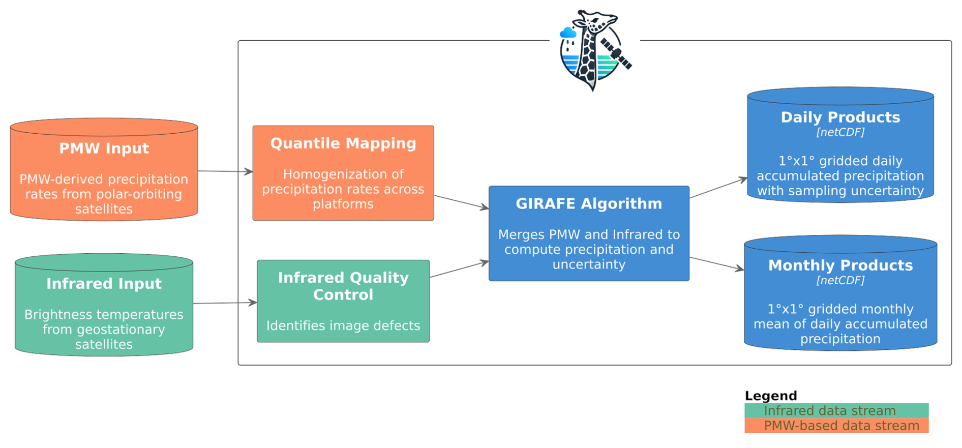
For latitudes inside 55° N/S, the GIRAFE algorithm merges the two input data streams towards the gridded daily accumulated precipitation output (Sect. 4.3.1). Grid cells outside of 55° N/S are based only on the PMW-based data stream (Sect. 4.3.2). The limit for using the infrared data stream is defined at 55° N/S because the distortion of the fields of view becomes larger towards the poles due to increasing viewing angles, leading to a trade-off between the improved temporal sampling and the declining accuracy of the infrared observations. This is similar to the latitudinal boundary used in GPCP v3.2 (Huffman et al., 2023a). The uncertainty module of the GIRAFE algorithm uses the variance in the daily precipitation fields and intermediate results of the merging module for a quantification of the number of independent samples to derive the sampling uncertainty associated with the daily accumulated precipitation product (Sect. 4.4). The monthly mean daily accumulated precipitation is derived directly from the daily fields (Sect. 4.5).
3.1 Geostationary Level-1 infrared brightness temperatures
Passive infrared imagers on board at least five geostationary satellites have been providing a quasi-global coverage with the above-mentioned latitudinal restrictions. While there have been gaps in the constellation of geostationary satellites prior to 1998, it is complete in the time period considered for GIRAFE v1 (2002 onwards). All infrared imagers feature an infrared channel between 10.3 and 11.5 µm with spatial resolutions between 2 and 5 km at nadir, with temporal samplings between 10 and 30 min, including partial scans of the Northern and Southern hemispheres. Figure 2 provides an overview of the available platforms. Instrument details are summarised in Table 1.
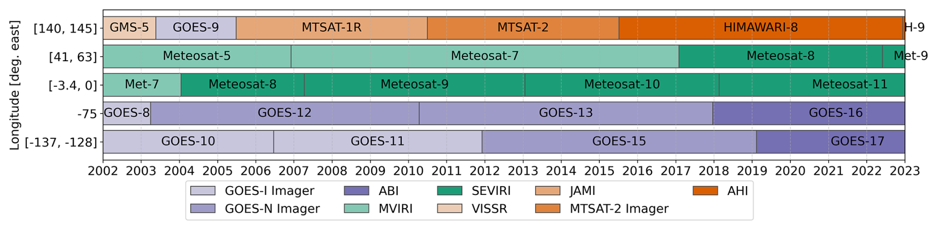
Figure 2Geostationary platforms and their temporal coverage as used in GIRAFE v1. The respective instruments are colour-coded; see also Table 1. The labels on the vertical axis indicate the sub-satellite longitude range of the platforms in the respective position. H-9 = HIMAWARI-9, Met-9 = Meteosat-9.
Instantaneous infrared Tb observations (Level-1) for the entire time series have been collected from the corresponding agencies (EUMETSAT, NOAA, JMA/JAXA). In principle, despite GIRAFE being designed for climate applications, the infrared Tb observations are not required from high-quality intercalibrated fundamental CDR (FCDR) archives: long-term drifts in the infrared observations are intercepted by the training of the infrared observations with PMW-derived precipitation rate estimates over short windows (1 d periods; see Sect. 4.3.1). Therefore, non-intercalibrated data from operational archives may be used. Operational calibration coefficients are applied to convert raw image counts to Tbs. As one available exception, EUMETSAT's FIDUCEO MVIRI FCDR (Rüthrich et al., 2020a–c) for Meteosat First Generation is preferred over the operational data due to the improved (inter-)calibration and the accompanying quality control. Where possible, future GIRAFE versions will rely on more infrared datasets of FCDR quality.
Table 1Geostationary instruments used in GIRAFE v1.
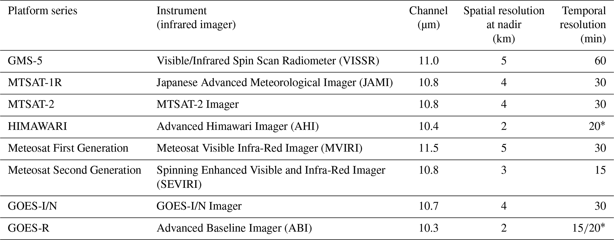
* Reduced temporal resolution to limit computation time.
3.2 Passive microwave-based Level-2 precipitation rate estimates
The PMW-derived database used for GIRAFE v1 is diverse in the sense that we use the data obtained from nine different types of PMW radiometers operated on a series of 19 different LEO satellites, processed by three different algorithms. The diversity in their retrievals, such as the frequency distribution of the occurrence of precipitation rates, makes the pre-processing described in Sect. 4.2 necessary. Figure 3 lists all PMW satellites that feed into GIRAFE v1. Table 2 provides details on the instruments. The respective retrieval algorithms and data sources are detailed in Sects. 3.2.1–3.2.3.
Table 2Overview of PMW instruments used in GIRAFE v1. Figure 3 illustrates the deployment of these instruments and their usage in GIRAFE v1. Lower maximum latitudes imply orbits further away from sun-synchronicity, hence providing a more diverse diurnal sampling.
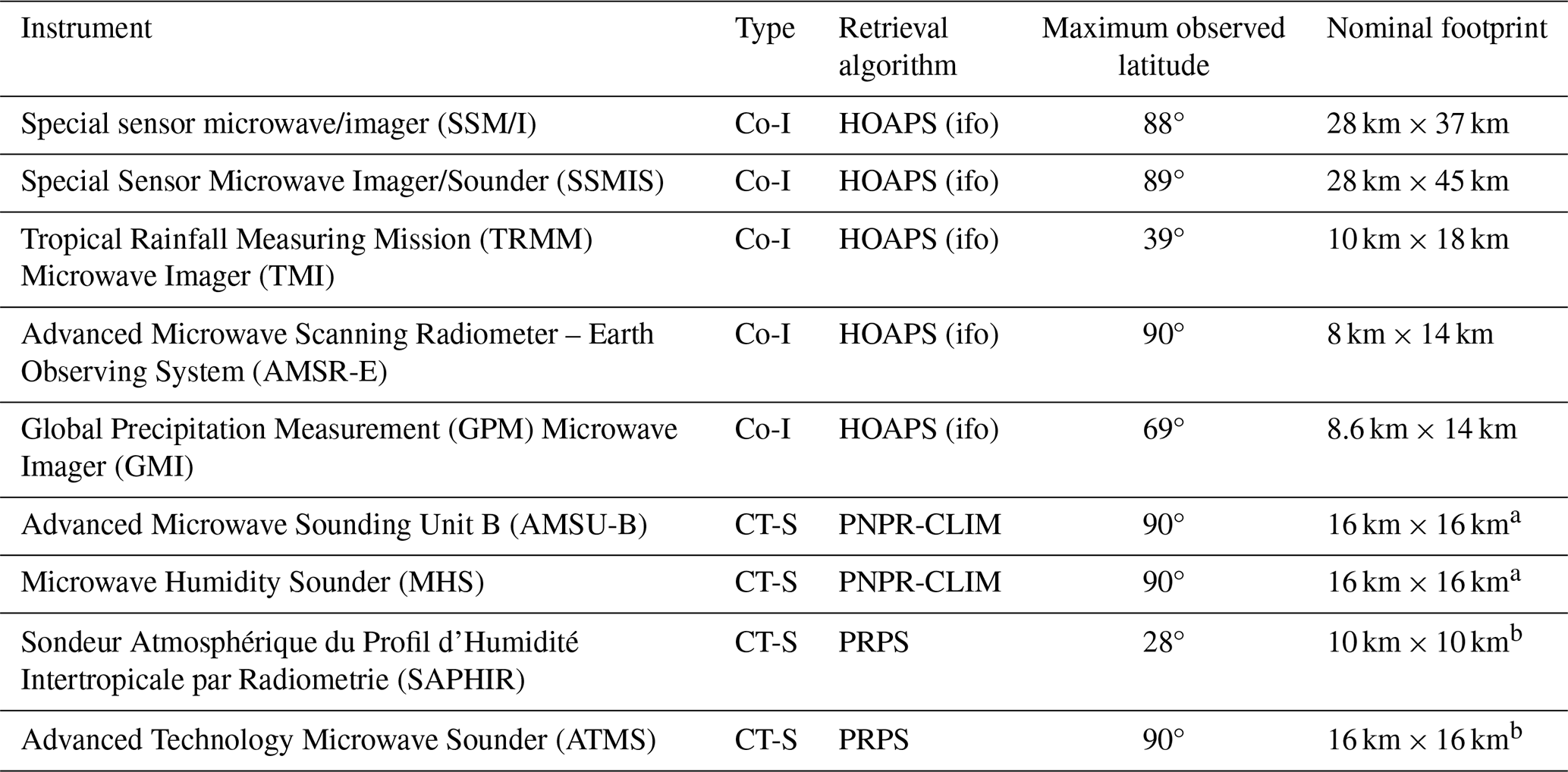
Co-I = Conical-scanning PMW imager; CT-S = Cross-track scanning PMW sounder; ifo = ice-free ocean only. a Valid at nadir; distortion at higher scan angles accounted for in the downstream GIRAFE processing. b Multiples of DPR resolution; no distortion assumed at higher scan angles.
3.2.1 HOAPS
Instantaneous precipitation rates from PMW imagers over ice-free ocean are based on the Hamburg Ocean Atmosphere Parameters and fluxes from Satellite (HOAPS) dataset. For the precipitation rate retrieval, an artificial neural network (ANN) trained with precipitation rates retrieved from assimilated Tbs in a 1D-Var scheme from the European Centre for Medium Range Weather Forecast (ECMWF) has been designed to derive a statistical retrieval from SSM/I and SSMIS (SSMI(S) from here) Tbs (Andersson et al., 2010). The resulting HOAPS precipitation retrieval is a statistical algorithm that depends only on Tbs as input data. As argued by Andersson et al. (2010), precipitation rates below 0.3 mm h−1 are set to 0 due to their low signal-to-noise ratio, i.e. where the microwave signatures possibly stemming from (wind-driven) surface emission modulations or the presence of cloud liquid water or water vapour are misinterpreted as those of precipitation or vice versa (e.g. Ferraro et al., 1998). The ANN is designed for PMW imager Tbs of the CM SAF SSMI(S) FCDR (Fennig et al., 2020) at the resolution of the 37 GHz channel of the respective sensor.
Instantaneous precipitation rates from PMW imagers TMI, GMI, and AMSR-E intercalibrated to the SSMI(S) FCDR are also retrieved with the above-mentioned ANN. As these PMW imagers have a higher resolution compared to SSMI(S), related footprints of the L1C data are averaged to match the SSMI(S) footprints. Additionally, based on Olson et al. (2001), a correction factor for the level of mixing of convective and stratiform precipitation was developed using polarisation differences at the inter-calibrated 85 GHz (V–H) vs. the average 85 GHz Tbs.
3.2.2 PNPR-CLIM
The Passive microwave Neural network Precipitation Retrieval for CLIMatological applications (PNPR-CLIM; Bagaglini et al., 2021) has been developed within the Copernicus Climate Change Service (C3S) programme for deriving instantaneous precipitation rates from Tbs observed by AMSU-B and MHS cross-track scanning radiometers as provided in the respective FIDUCEO FCDR v4.1 (Hans et al., 2019) over land and ocean. PNPR-CLIM consists of two ANNs, one for the detection of precipitation in AMSU-B/MHS Tbs and the other for its quantification. Both are trained with high-quality precipitation observations by the combined GMI and Dual-frequency Precipitation Radar (DPR) instruments on board the GPM Core Observatory (GPM-CO) (2B-CMB V06A data; Grecu et al., 2016), collocated with FIDUCEO MHS data. In addition to instantaneous Tbs and respective differences between selected channels, the inputs to the algorithm are the scan angle, a global land/sea mask for surface classification, and ERA5 fields (Hersbach et al., 2020) at 0.25° and monthly resolution for the auxiliary input variables, namely, 2-metre temperature, freezing level, total precipitable water vapour, snow depth, and sea-ice concentration. In the presence of deep convection – detected in Tb differences from the 183 GHz sounding channels – the precipitation rates are calibrated to match the distribution of the high-resolution ground-based Multi-Radar-Multi-Sensor System dataset in North America (Zhang et al., 2016), similarly to the quantile mapping applied here (Sect. 4.2). Indicators of the degradation of the quality, such as the presence of sea ice or snow (based on ERA5; see also Sect. 4.6), are provided as quality flags. With the respective FIDUCEO FCDR ending in 2017, PNPR-CLIM was adapted for the NASA PPS L1C MHS observations from 2018 onwards, with only negligible discontinuities in spatiotemporally averaged per-satellite precipitation.
3.2.3 PRPS
The Precipitation Retrieval and Profiling Scheme (PRPS) (Kidd et al., 2021) uses L1C observations from PMW sensors (ATMS and SAPHIR in the case of GIRAFE v1) to retrieve L2 precipitation estimates over both land and ocean. PRPS relies on observational data with minimal, if any, input of ancillary data. PRPS-SAPHIR was developed for operational use alongside the Goddard Profiling scheme (GPROF; Kummerow et al., 2011) and is obtained from NASA GPM repositories (see Sect. 6). PRPS uses an a priori database that is based upon matched Tb observations of SAPHIR or ATMS and aggregated DPR observations (2B-CMB v06 A; see Sect. 3.2.2) with a maximum temporal difference of 5 min and geolocation within 2.5 km. For a given SAPHIR or ATMS observation (set of Tbs from different channels), PRPS finds the six closest matched database entries at similar sensor scan positions and averages the respective DPR-based precipitation rates. PRPS-ATMS reveals unrealistically high precipitation rates over ice-covered surfaces, so that respective observations are discarded according to the Operational Sea Surface Temperature and Ice Analysis (OSTIA) at 0.05° resolution (Good et al., 2020) and for static masks over Antarctica, Lake Baikal, and the Aral Sea. This step is not necessary for PRPS-SAPHIR because of its low-latitude coverage (Table 2).
In this section, the algorithms and their scientific basis for pre-processing and merging of the input data streams are introduced. The GIRAFE algorithm for daily accumulated precipitation (Sect. 4.3) and the respective sampling uncertainty (Sect. 4.4), as well as the upstream infrared quality control (Sect. 4.1), are based on the methods used for the Tropical Amount of Precipitation with an Estimate of ERrors (TAPEER) algorithm and product (Chambon et al., 2013; Roca et al., 2018), developed for the exploitation of observations by the Megha-Tropiques satellite mission. The pre-processing of PMW-based precipitation rates (Sect. 4.2) is necessary because of the diversity of the PMW database (Sect. 3.2). Sections 4.5 and 4.6 discuss the post-processing steps of aggregating the monthly resolved product and the flag for identifying the quality-reducing presence of surface snow or ice.
4.1 Infrared quality control
Except for the MVIRI FIDUCEO FCDR, we use operational geostationary datasets (Sect. 3.1), which require quality control to make them suitable for climate applications. Erroneous scan lines in infrared images are flagged using a radiometric quality control algorithm (Szantai et al., 2011) and are subsequently ignored in the GIRAFE algorithm.
4.2 Quantile mapping of PMW-based precipitation rate estimates
The various sources of the PMW-based input stream require a homogenisation procedure. This is particularly important because of the use of a detection threshold (Sect. 4.3), as a mismatch between satellites or retrieval algorithms will have a strong impact on the training of the infrared observations in the final GIRAFE output. Here, quantile mapping is applied, which is a common method for constructing precipitation datasets from a variety of PMW-based input. For example, Huffman et al. (2007), Tan et al. (2021), or Yamamoto and Kubota (2022) use quantile mapping or methods, although the details vary. We derive the mapping from non-collocated instantaneous (Level-2) precipitation rate estimates and apply it to these same instantaneous observations.
Observations by SSMIS on board DMSP-F17 (algorithm HOAPS) and MHS on board METOP-A (algorithm PNPR-CLIM) are selected as targets for the quantile mapping procedure over ocean and land, respectively (Fig. 3), because of the long and stable time series from these sensors. Instantaneous precipitation rates r observed by other satellites according to the respective retrieval algorithms are converted to match the distributions of the target platforms:
Here, f and g are the cumulative probability density functions of the precipitation rates from the mapped and the target satellite, respectively. The mapped precipitation rates, rT, are used in the PMW-based input stream to GIRAFE. As the distributions representing f and g depend on precipitation regimes and overall climatological situations, they are constructed separately for each month of the year and for each surface type (land and ocean, hence two target satellites) by counting the number of instantaneous observations in respective precipitation rate bins and then accumulating along the precipitation rate dimension. Also, the distributions are collected separately over bands in latitude (8° spacing at the Equator to 20° at higher latitudes) and longitude (six bands in total, separating continents). Besides the definition of distributions by month of the year, no time dependency is implemented, i.e. the distributions are based on all available years from the respective satellite between 2002 and 2020. This also implies that this method impacts the homogeneity and stability of the GIRAFE v1 time series only by removing average inter-sensor discontinuities, but not any drifts of single satellites. In the presence of a strong drift, residual discontinuities may occur when the respective satellite joins or leaves the constellation. However, based on the findings in Sects. 5.3 and 5.4, there is no evidence for such situations when comparing against other (quasi-)global datasets over the regions specified in our homogeneity and stability analyses.
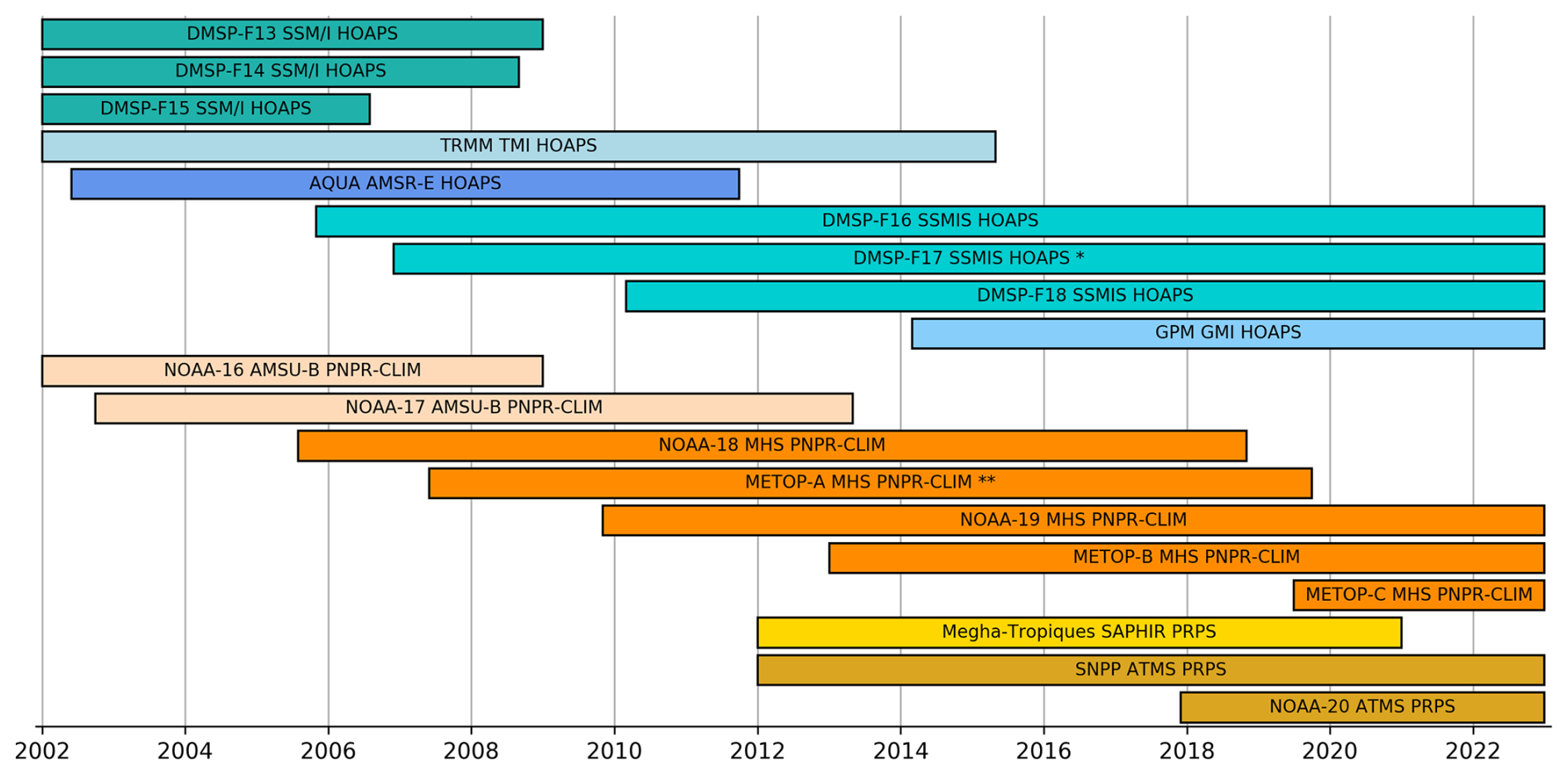
Figure 3Overview of satellites bearing PMW sensors and their temporal availability used in GIRAFE v1. The labels indicate the satellite, instrument, and corresponding precipitation retrieval algorithm; see also Table 2. Identical instruments are identified by the same colour. * Quantile mapping target over ocean (Sect. 4.2); ** quantile mapping target over land.
Months with strong El Niño–Southern Oscillation (ENSO) amplitudes as per the MEI v2 index (Wolter and Timlin, 2011) are discarded during the collection of distributions, due to reportedly high dependency of HOAPS on these conditions (e.g. Masunaga et al., 2019). Strong ENSO events are identified by the MEI v2 index surpassing 1.0 (El Niño) or falling below −1.25 (La Niña). These thresholds have been defined ad hoc.
The mapping as per Eq. (1) is substituted by an identity mapping (i.e. effectively no quantile mapping) in latitudes above 70° N/S during the hemispheric winter half-year, due to few or no (non-zero) observations over snow and ice in either of the three sub-databases (HOAPS, PNPR-CLIM, PRPS; Sects. 3.2.1–3.2.3), and in latitude/longitude boxes with less than 3 % of the respective surface type (land/ocean), due to few observations possibly leading to spurious distributions. Finally, the mapping is interpolated in narrow transitions between the above-mentioned latitude and longitude bands in order to avoid unphysical discontinuities at these boundaries. The positive homogenising effect of the quantile mapping procedures is illustrated in Appendix A.
Observed Tbs are often affected by geometric distortions, leading, among others, to a very low spatial resolution, especially in the case of cross-track scanning microwave sounders. Therefore, the five outer scan positions for AMSU-B and MHS are discarded for both the construction of the distributions and the later use in the merging procedures, according to PNPR-CLIM quality flagging. For the other cross-track scanning sensors ATMS and SAPHIR, only the outer two scan positions are discarded because the sensor resolution is prescribed by the PRPS algorithm (Table 2). Microwave imagers are less affected due to their conical scanning geometry.
Data from single satellites during periods when Tbs and hence precipitation rate estimates are contaminated or show a strong trend not detected by other satellites are discarded for both the quantile mapping and the later use in the merging. These periods are detected in a non-automated fashion by eye in per-satellite anomaly time series of monthly means over different regions (tropics, northern/southern extra-tropics, and separately over land and ocean; see Niedorf et al., 2024b). Such trends occur mostly at the start or towards the end of the lifetime of a satellite. The respective removals lead to the periods detailed in Fig. 3, which, in these cases, deviate from the actual satellite uptime values. Data from a single shorter period of contamination for NOAA-19 in October 2017 as reported by Sanò et al. (2021) were also removed. No further quality control was carried out on the PMW-based data. The utilisation of mostly quality-controlled FCDR sources for PMW Tb observations in GIRAFE gives confidence that contaminations are rare, but their occurrence cannot be entirely excluded.
4.3 Derivation of daily accumulated precipitation
The estimation of accumulated precipitation is based on the TAPEER algorithm (Chambon et al., 2013). The merging of PMW and infrared observations inside 55° N/S follows the GOES Precipitation Index technique (Arkin, 1979), more specifically the Universally Adjusted GOES Precipitation Index (Xu et al., 1999); see Sect. 4.3.1. for details. This approach separates the daily accumulated precipitation (Pacc) in a (1DD) grid cell into the conditional precipitation rate (R, in mm h−1) and the precipitation fraction (F, unitless) in this cell:
hence assuming that, if it rains in the grid cell, it occurs at a constant average intensity. The derivation of R is based only on the PMW database:
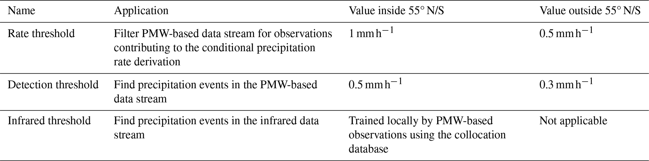
Here, the index i specifies instantaneous PMW observations in the (3DD) environment centred around the 1DD grid cell, regardless of the source satellite/sensor, for which the precipitation rate estimates ri lie above a pre-defined rate threshold (Table 3). The choice of 3DD for the size of the environment optimises the frequency distributions of 1DD precipitation rates simultaneously with the respective rate thresholds and detection thresholds (see below) when compared to established datasets. The respective footprint areas ai (Table 2) are used for linearly weighting the precipitation rate estimates because observations of large areas are expected to be more representative for the entire 3DD environment than those of smaller ones. The derivation of F and the rate threshold for the derivation of R depend on whether the 1DD grid cell is inside (Sect. 4.3.1) or outside (Sect. 4.3.2) of 55° N/S.
Table 3Overview of the thresholds used for the computation of the conditional precipitation rate R and the precipitation fraction F during the merging in the GIRAFE algorithm.
One day is defined from 00:00:00 UTC to 00:00:00 UTC on the next day in the official product discussed here. However, for users who need to rely on a different local time equivalent, unofficial variants with periods shifted by 6, 12, and 18 h exist and are available upon request (see Sect. 6). Figure 4 shows the resulting intermediate results for F and R (panels a and b) for 1 exemplary day, as well as the final daily accumulated precipitation Pacc as per Eq. (2) in panel c.
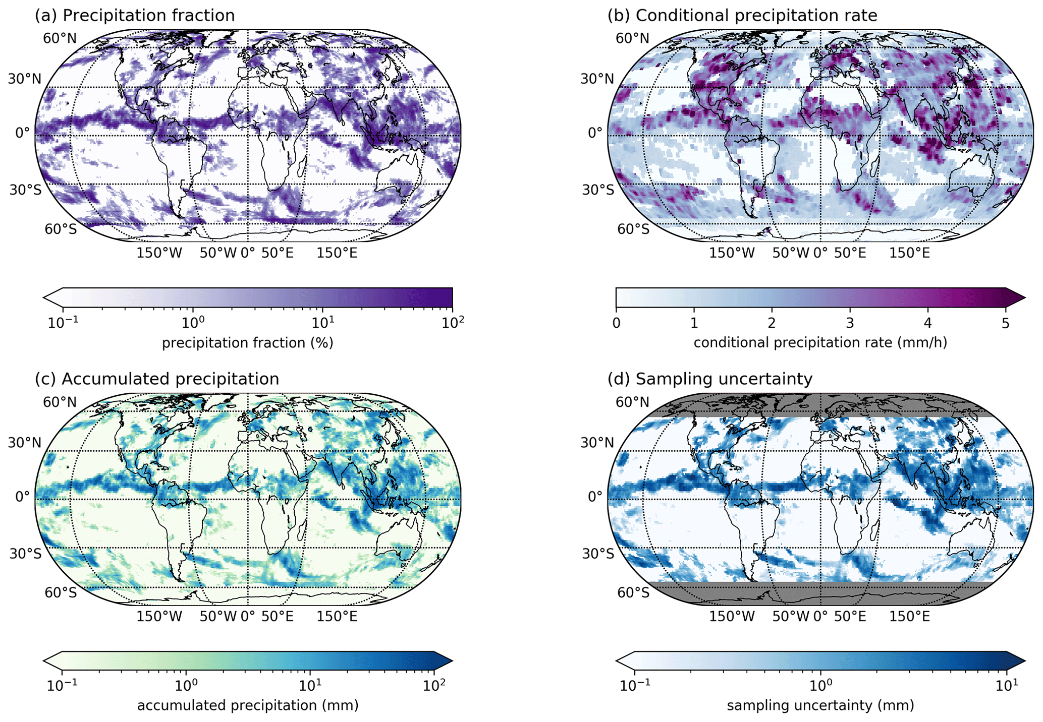
Figure 4Example fields for the GIRAFE v1 precipitation fraction F (panel a), the conditional precipitation rate R (panel b), the resulting daily accumulated precipitation Pacc (panel c), and the sampling uncertainty σS (panel d) on 13 July 2021. The minimum value of the fields illustrated in panels a, c, and d using logarithmic colour scales is 0.
4.3.1 Inside 55° N/S (merging)
At latitudes below 55° N/S, where infrared observations from geostationary satellites are utilised, the GIRAFE algorithm derives the precipitation fraction F from the merged infrared and PMW-based data streams following the Universally Adjusted GOES Precipitation Index technique (Xu et al., 1999). For a given 1DD grid cell, the GIRAFE algorithm finds collocated observations in the infrared and PMW-based data streams in a environment centred around the 1DD grid cell. Observations are ingested into the collocation database (i) if the infrared observation lies inside the much larger footprint ellipse of the respective PMW observation (spatial criterion; see Table 2) and (ii) if the infrared observation and the PMW observation were recorded within the duration of one geostationary infrared imager scan cycle (temporal criterion; see Table 1). The infrared observations are processed at the sensor-specific resolution and sampling rate; differences between the sensors do not impact the results systematically because of the above-mentioned training that is local in space and time.
Based on this collocation database, a threshold for the detection of precipitation in the infrared Tbs is derived (“infrared threshold”, Table 3) for the 1DD grid cell. For this, the fraction of PMW-based precipitation rate estimates exceeding the detection threshold of 0.5 mm h−1 (Table 3) in the collocation database is determined. The infrared threshold is then derived as the quantile in the infrared Tb distribution in the collocation database, which corresponds to this PMW-based precipitation fraction, cf. Fig. 5. The precipitation fraction, F, is computed as the fraction of precipitation events (Tb below the derived infrared threshold) in all infrared observations falling into the 1DD grid cell.
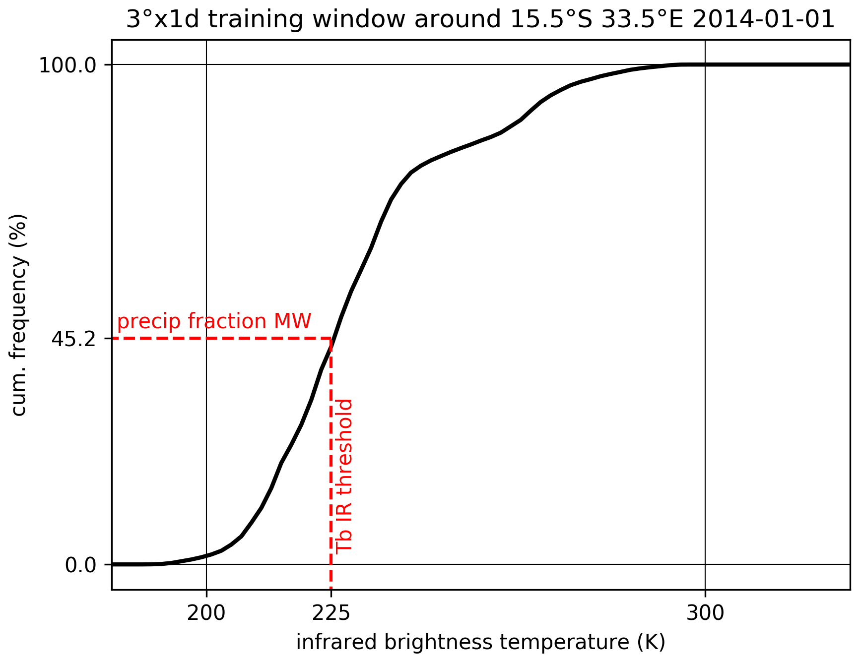
Figure 5Example derivation of the infrared threshold (vertical red dashed line) based on the PMW-based precipitation fraction (horizontal red dashed line) and the distribution of infrared (IR) Tbs (thick black line), both in the collocation database of the respective 1DD grid cell.
Inside 55° N/S, the conditional precipitation rate for a 1DD cell is computed using a rate threshold of 1.0 mm h−1, which was found to bring the overall frequency distributions of daily accumulated precipitation in GIRAFE v1 closest to established datasets in early results – in tandem with the 0.5 mm h−1 detection threshold used for the training of the infrared threshold (see above) and the 3DD environment for the averaging of the conditional precipitation rate.
4.3.2 Outside 55° N/S
Where no infrared data are used, the GIRAFE algorithm relies only on the PMW-based data stream as follows: the precipitation fraction F is the fraction of PMW-derived precipitation rates exceeding 0.3 mm h−1 in the 1DD grid cell (Table 3). This threshold for the detection of precipitation in the PMW data stream is lower than that inside the 55° N/S region (0.5 mm h−1; see Sect. 4.3.1) due to precipitation occurring at lower rates at higher latitudes in general. In this respect, GIRAFE deviates from the TAPEER methods established by Chambon et al. (2013), who did not consider regions of the planet where infrared observations from geostationary satellites cannot be used.
The 1DD conditional precipitation rate is computed in the same way as inside 55° N/S but using a rate threshold of 0.5 mm h−1 (Table 3), which proved optimal in reproducing frequency distributions of established datasets in tandem with the 0.3 mm h−1 detection threshold and the 3DD environment for the averaging of the conditional precipitation rate (see above) in an early version.
4.4 Daily sampling uncertainty
The GIRAFE sampling uncertainty is based on instantaneous precipitation fields that are obtained from the infrared Tb observations by applying the 1DD infrared threshold as explained in Sect. 4.3.1. It is therefore only available inside the 55° N/S latitude band covered by geostationary satellites. These instantaneous precipitation fields can take two different values: 0 for infrared Tbs exceeding the infrared threshold (no precipitation) or the conditional precipitation rate R otherwise. Following Roca et al. (2010) and Chambon et al. (2013), the sampling uncertainty, σS, is computed as
with being the standard deviation of the binary infrared-based precipitation field in the 1DD cell. With strong correlations present between neighbouring infrared pixels, the number of independent observations Nind in Eq. (4) is well below the number of available infrared observations. It is estimated as
where A is the area of the 1°×1° grid cell, T=24 h is the temporal extent of the grid cell, and d and τ are the decorrelation scales of the precipitation signal in space and time, respectively. These decorrelation scales are estimated separately from exponential fits to variograms of the binary infrared-based precipitation fields in the respective dimensions.
This uncertainty measure is useful when satellite and ground-based estimates are compared as detailed, for instance, in Roca et al. (2010) and Gosset et al. (2018). It has also been successfully used to assess the sensitivity of the satellite products to the configuration of the microwave constellation (Roca et al., 2018; Oliveira and Roca, 2022). Dataset-specific uncertainties could also be very useful in the context of hydrological modelling applications, as an added value for exploring different scenarios of river discharge simulations through ensembles constructed by otherwise offline estimates of precipitation uncertainty (e.g. Paiva et al., 2013, Wongchuig et al., 2024), particularly in intertropical basins, which are subject to strong spatiotemporal variability of precipitation.
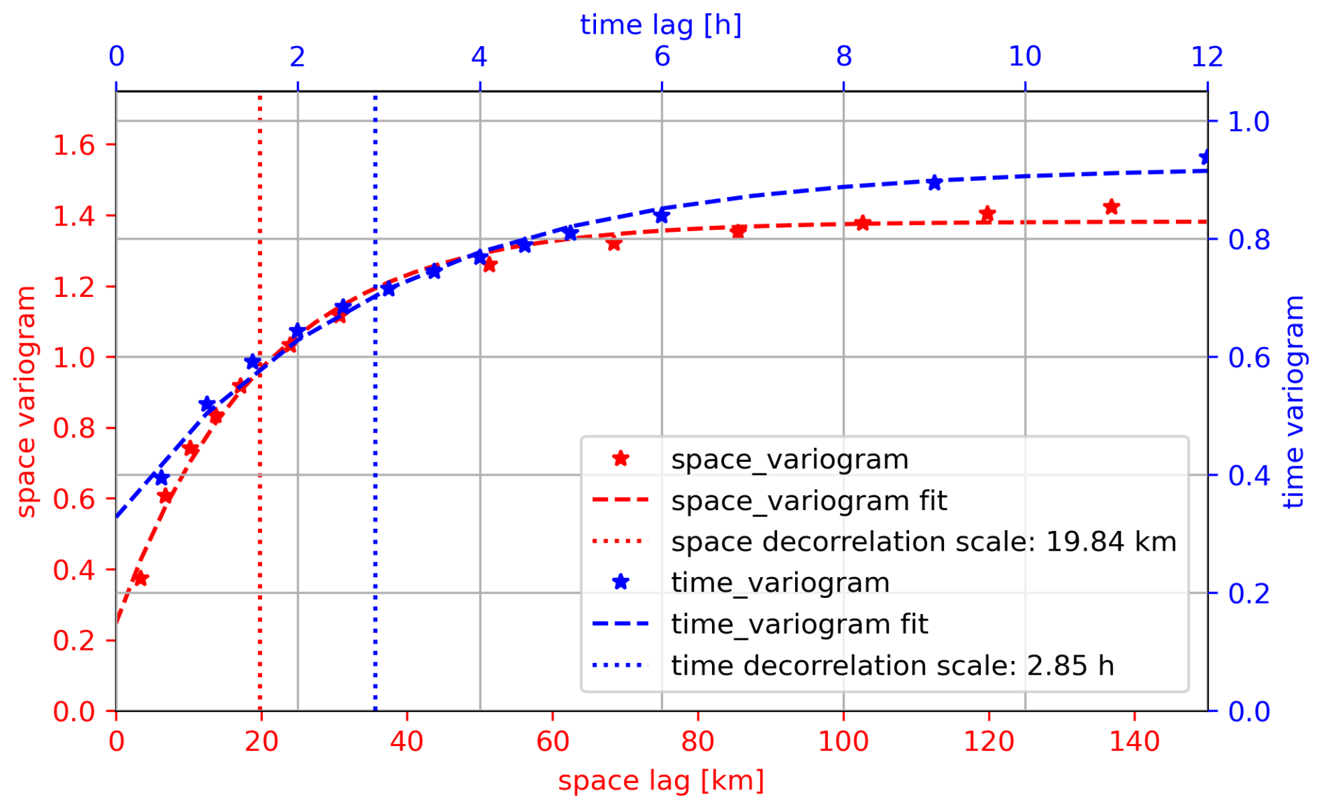
Figure 6Example space variogram (red) and time variogram (blue) of a environment. The 5°×5° box is centred at 12.5° N/27.5° W (tropical East Atlantic Ocean), and the time period covers 11–20 July 2021. Red axes (left and bottom) belong to the space variogram, whereas blue axes (right and top) are assigned to the time variogram. Stars mark the computed experimental variograms, and dashed lines show the respective fit. The dotted vertical lines illustrate the fitted decorrelation scales in space (blue, 19.84 km) and time (red, 2.85 h).
The variograms are collected over larger fixed (i.e. non-moving) environments, thereby increasing the underlying databases to form a larger statistical ensemble rather than covering only few events. The variograms in spatial dimensions are first computed per scan in 5°×5° cells based on spatial increments in the scan line and scan position directions only, and then the per-scan variograms over the 10 d period are averaged. Conversely, the temporal variograms are first computed per geostationary pixel over the 10 d period based on differences in scan times, and then the per-pixel variograms are averaged over the 5°×5° boxes. For both types of variograms, the binary infrared-based precipitation fields are sampled to coarser resolutions, depending on sensor specifications (scan frequency and spatial resolution at nadir; see Table 1), roughly matching a temporal resolution of 1 h and a spatial resolution of 5 km (nadir) for the spatial variograms and 30 min and 15 km for the temporal variograms, respectively. In general, this resampling harmonises the available resolutions of different sensors as far as possible. However, the lowest resolution is not always taken as the target to not reduce the quality of the more advanced instruments. Therefore, outliers such as the VISSR sampling frequency of 60 min cannot be overcome, and the resulting larger minimum lag between two observations for, e.g., VISSR may have a systematic effect on the resulting decorrelation scales. Figure 6 shows an example space variogram and time variogram of a environment and its respective fits and decorrelation scales.
The fit procedure works well for truly exponentially shaped variograms, such as the ones shown in Fig. 6. There are situations in which the variograms cannot be calculated or have irregular shapes, for example, falling below the plateau at higher lags or an alternation of high and low values at low lags instead of a monotonous increase, possibly due to many missing infrared scenes or in arid settings. This typically leads to implausibly low or high or entirely missing decorrelation scales, due to numerical instabilities in the fitting routine in the latter case. These situations are filtered by identifying cases for which the decorrelation scale is below the minimum lag, above the maximum lag, or not retrieved. In order to avoid gaps, the respective values are replaced by climatological values (20 km for spatial and 1.5 h for temporal decorrelation). These values are relatively well aligned with the most frequent values of the variogram fits in both GIRAFE v1 and TAPEER v1.5 (Figs. 5–13 in Konrad et al., 2024). A flag is provided that identifies these situations and allows the rejection of respective derived uncertainty estimates.
Figure 4 shows the resulting sampling uncertainty as per Eqs. (4) and (5) for 1 exemplary day in panel d.
4.5 Monthly aggregation of daily accumulated precipitation
For the convenience of users who are interested in an average monthly precipitation, the global 1DD accumulated precipitation fields (Sect. 4.3) are averaged along the temporal dimension over each month, yielding (1DM) gridded global fields. The number of days available for averaging is provided for each 1DM grid cell, as well as a flag that informs users whether there are more than 10 d or more than 4 consecutive days missing in the 1DM grid cell, in which case the 1DM value is non-compliant with guidelines by the World Meteorological Organization (WMO, 2017). The daily sampling uncertainty is not propagated to the 1DM resolution, due to the unknown day-to-day uncertainty correlation.
4.6 Snow/ice flag
With HOAPS not providing PMW-derived precipitation rates over ice- or snow-covered areas, PRPS output being specifically filtered for these situations (Sect. 3.2.3), and PNPR-CLIM being reportedly weak in these situations (Bagaglini et al., 2021), a snow/ice flag (SIF) is introduced following the PNPR-CLIM quality flag setting for snow and ice cover: ERA5 snow depth and sea-ice concentration (Hersbach et al., 2020) above 0 in a 3DD environment (matching the maximum extent of the GIRAFE environments) around a 1DD grid cell indicate a probable degradation of the data quality in GIRAFE v1; hence, SIF=1 and SIF=0 otherwise for the 1DD grid cell. For the monthly GIRAFE v1 data, the number of days with SIF=1 are counted for each 1DM grid cell.
GIRAFE v1 comes with an extensive validation report (Konrad et al., 2024) featuring comparisons against reference datasets and similar quasi-global datasets, a dedicated stability and homogeneity analysis, the verification of the plausibility of the uncertainties and the underlying decorrelation scales, and an analysis of missing values in the 1DD and 1DM datasets. In this section, we condense the information of this validation report and refer the interested reader to the validation report for the extended analysis. Particular emphasis is put on the homogeneity analysis (Sect. 5.3), the stability analysis (Sect. 5.4), and the analysis of the scaling of daily extreme precipitation with sea surface temperature (SST), which was not featured in the validation report (Sect. 5.5). Finally, Sect. 5.6 illustrates how the GIRAFE v1 sampling uncertainty resembles the validated TAPEER v1.5 uncertainties.
We focus on the assessment of the 1DD dataset of the GIRAFE v1 CDR. In order to put the GIRAFE v1 CDR results in perspective, the validation activities presented in Sect. 5.1 are carried out also for the established (quasi-)global satellite-based datasets: Global Precipitation Climatology Project (GPCP) v3.2 (Huffman et al., 2023a), Climate Prediction Center Morphing Technique (CMORPH) v1 (Xie et al., 2017), Integrated Multi-satellitE Retrievals for GPM (IMERG) v6 (Huffman et al., 2020) and v7 (Huffman et al., 2023b; not present in the previously mentioned validation report by Konrad et al., 2024), and Global Satellite Mapping of Precipitation (GSMaP) NRT v8 (Kubota et al., 2007; not present in the previously mentioned validation report by Konrad et al., 2024). The reanalysis dataset ERA5 (Hersbach et al., 2020) is also included in these comparisons. GPCP v3.2 is corrected towards rain gauge observations over land, which is not the case for GIRAFE v1. There are both corrected and uncorrected versions for CMORPH (CRT and RAW), IMERG (FC and FU), and GSMaP (with and without “gauge” in the labels below). Where feasible, we also include TAPEER v1.5 (Roca et al., 2018). For the homogeneity and stability analyses (Sects. 5.3 and 5.4), we also use the TRMM Multi-satellite Precipitation Analysis (TMPA) 3B42 v7 (Huffman et al., 2016) and the Global Precipitation Climatology Centre (GPCC) v2022 (Ziese et al., 2022) datasets. All datasets are retrieved at 1DD resolution from the Frequent Rainfall Observations on GridS (FROGS) archive (Roca et al., 2019a).
Following, for example, Gosset et al. (2018), we rely on established indicators of quality for assessing the various datasets, namely, bias (mean difference), bias-corrected root-mean-square difference (bc-RMSD), correlation coefficient (CC), detection statistics (hit rate, HR; probability of detection, POD; false alarm rate, FAR; and Heidke skill score, HSS), and the frequency of error bar overlap (FEBO). Apart from the detection statistics, no distinction is made between non-zero and no precipitation during the computation of the indicators. Where spatial dimensions are collapsed during the computation of the bias and bc-RMSD, each 1DD grid cell is weighted according to the area, i.e. proportional to sin(latitude). For the detection scores, the occurrence of precipitation in a 1DD grid cell is determined at 1 mm d−1, which is a common threshold for distinguishing dry and rainy days (e.g. Gosset et al., 2018).
5.1 Validation
The analyses in Sects. 5.1.1 and 5.1.2 are considered validations in the sense that the validating local dataset AMMA-CATCH and regional dataset EURADCLIM are high-resolution and high-accuracy. These datasets are limited both in time and more so in space. Already between these two regions, the advantages and disadvantages of the validated datasets vary (see below). It can be expected that regions with other surface settings and climatological conditions will also see different results. Hence, the validation here can only be considered a sample rather than complete.
5.1.1 AMMA-CATCH
We use the data from a high-resolution, dense rain gauge network near Niamey, Niger, in the “African Monsoon Multidisciplinary Analysis – Couplage de l'Atmosphère Tropicale et Cycle Hydrologique” (AMMA-CATCH) dataset (Lebel et al., 2009) to validate GIRAFE v1 and the other above-mentioned (quasi-)global datasets. AMMA-CATCH has been used previously for the validation of satellite-based precipitation estimates (Gosset et al., 2018, and references therein). The Niamey gauge network covers the 1°×1° area around 13.5° N, 2.5° E and consists of 40–50 stations. Accumulated precipitation from these stations is extended to the entire 1°×1° area by kriging before aggregation over spatial dimensions. The respective kriging uncertainty is available. We use 24 h accumulations from 2002 to 2019. Precipitation in Niamey is governed by the West African Monsoon, so the comparison is carried out for observations between June and September. It is noted that according to the above specification of the Niamey network, the validation extends to only a single grid cell in spatial dimensions for GIRAFE v1.
Table 4Statistics from the 1DD comparison of the evaluated datasets against the AMMA-CATCH Niamey data. The comparison is carried out for June–September in 2002–2019 (exceptions: a 2002–July 2017; b 2012–2019).
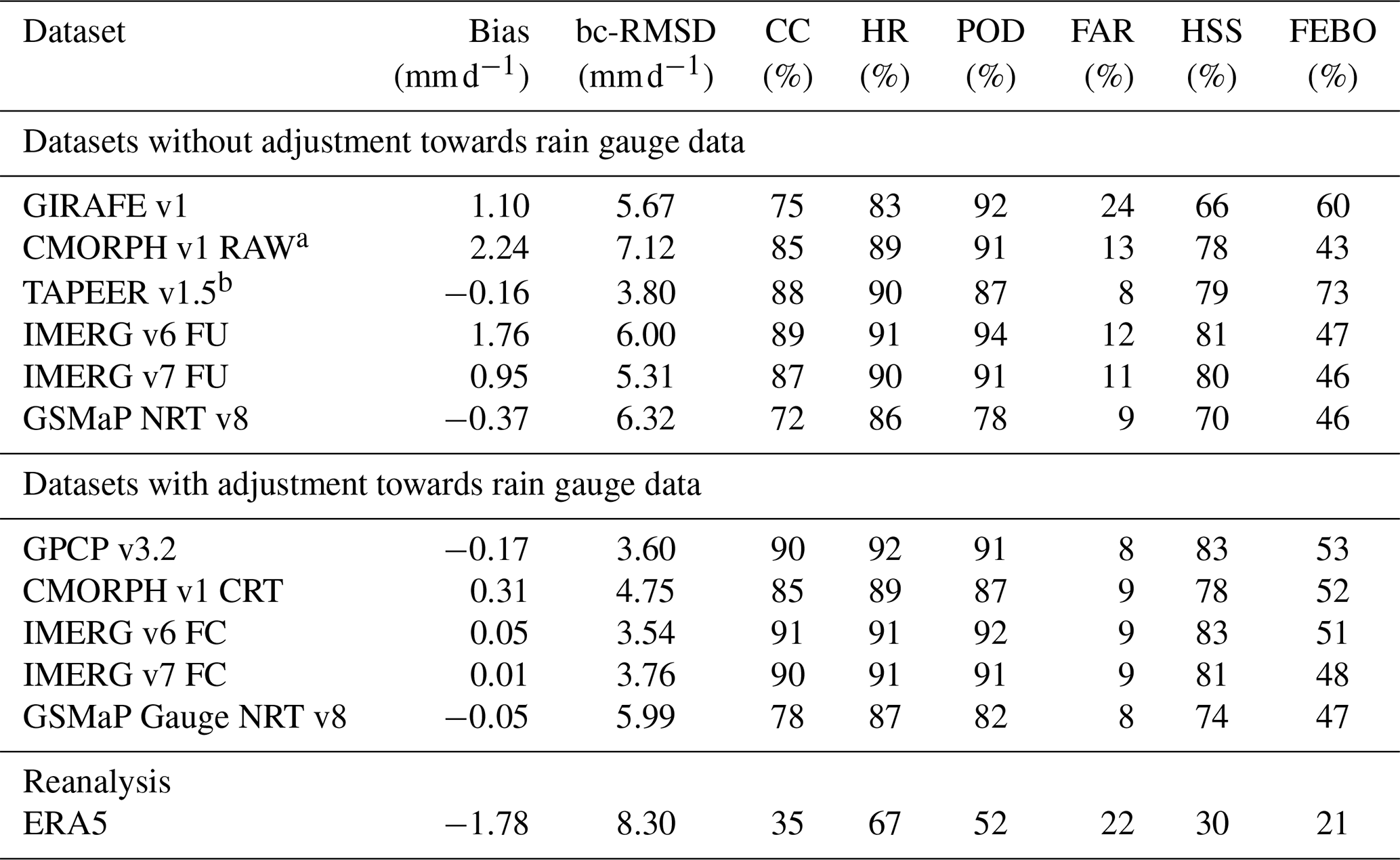
GIRAFE v1 has a bias and bc-RMSD against AMMA-CATCH that are in the range of other datasets that have not been adjusted to rain-gauge datasets (Table 4). While the POD of GIRAFE v1 is as high as in most other datasets, the GIRAFE v1 FAR is notably high, leading to lower scores also in terms of CC, HR, and HSS. The overestimation of precipitation in GIRAFE v1 is likely a feature of the PNPR-CLIM Level-2 data, which also produces increased precipitation over Africa (Bagaglini et al., 2021). The datasets that are adjusted to rain-gauge datasets usually perform better, indicating that future developments in GIRAFE context involving such an adjustment may also improve these scores. ERA5, except for the FAR statistic, performs weakest against the AMMA-CATCH dataset, possibly because no information relevant to precipitation is assimilated in the vicinity of the Niamey 1DD grid cell. In the absence of 1DD uncertainty information in the other datasets, except TAPEER v1.5, the FEBO of GIRAFE v1 is exceptionally high (60 %). The better performance of TAPEER v1.5 in this metric is likely a result of this dataset being designed for tropical conditions, of the generally lower bias, and of the better detection statistics. A more detailed discussion of the sampling uncertainty is given in Sect. 5.6.
5.1.2 EURADCLIM
We compare GIRAFE v1 and the above-mentioned (quasi-)global datasets to the 2013–2020 ground-based precipitation radar dataset EURADCLIM (Overeem et al., 2023). The 24 h accumulations are averaged from their native 2 km×2 km resolution to 1DD. An ad hoc sampling uncertainty is computed according to Eqs. (4) and (5), excluding the temporal dimension and with the default GIRAFE spatial decorrelation scale of 20 km. With the temporal sampling not being accounted for, the resulting uncertainty is likely to be underestimating the true sampling uncertainty in EURADCLIM. The comparison is restricted to 1DD grid cells south of 60° N for a fair comparison with CMORPH v1 and IMERG, which are (mostly) not available north of this latitude. The 528 remaining 1DD grid cells cover West and Central Europe, southern Scandinavia and the southern Baltic Sea, and parts of East Europe; see Appendix B for an illustration of the availability of mutual grid cells.
GIRAFE v1 tends to underestimate the amount of precipitation in EURADCLIM (low bias shown in Table 5) but remains largely in the range of the other unadjusted datasets. The overall bc-RMSD given in Table 5 is very close to the optimal values found in all datasets. This finding is confirmed in the comparison of spatial distributions of the bc-RMSD (Fig. 7). In general, GIRAFE v1, like the other datasets, sees an increased deviation from EURADCLIM over the Alps, the Pyrenees, the Balkans, the northern parts of Ireland and Great Britain, and the southern Norwegian coast. Most of these areas are mountainous, which makes the inference of precipitation from both satellites and ground-based radars more difficult.
Table 5Statistics from the 1DD comparison of the evaluated datasets against the EURADCLIM dataset. Only latitudes below 60° N are considered. The comparison is carried out for 2013–2020 (exception: * 2013–July 2017).
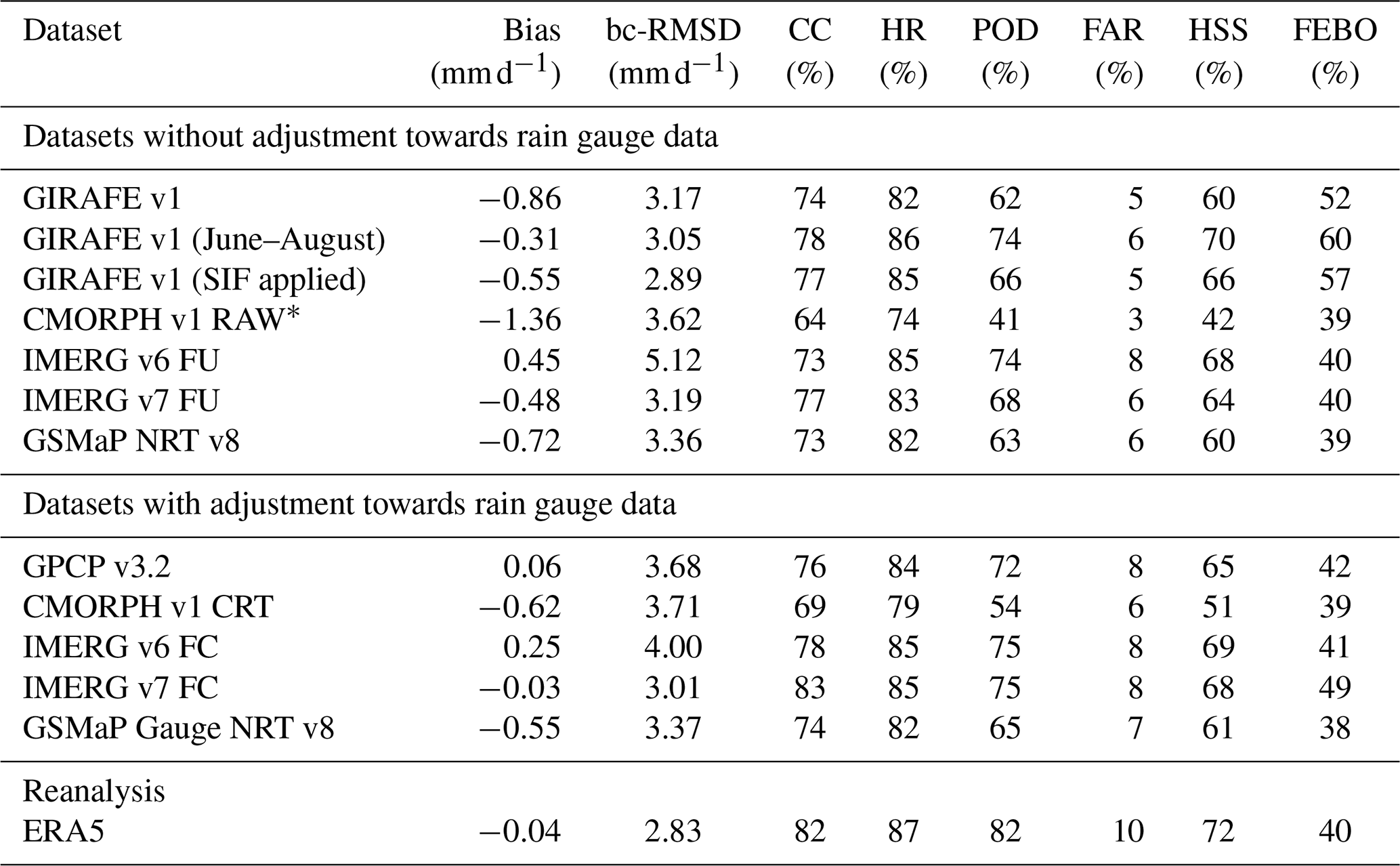
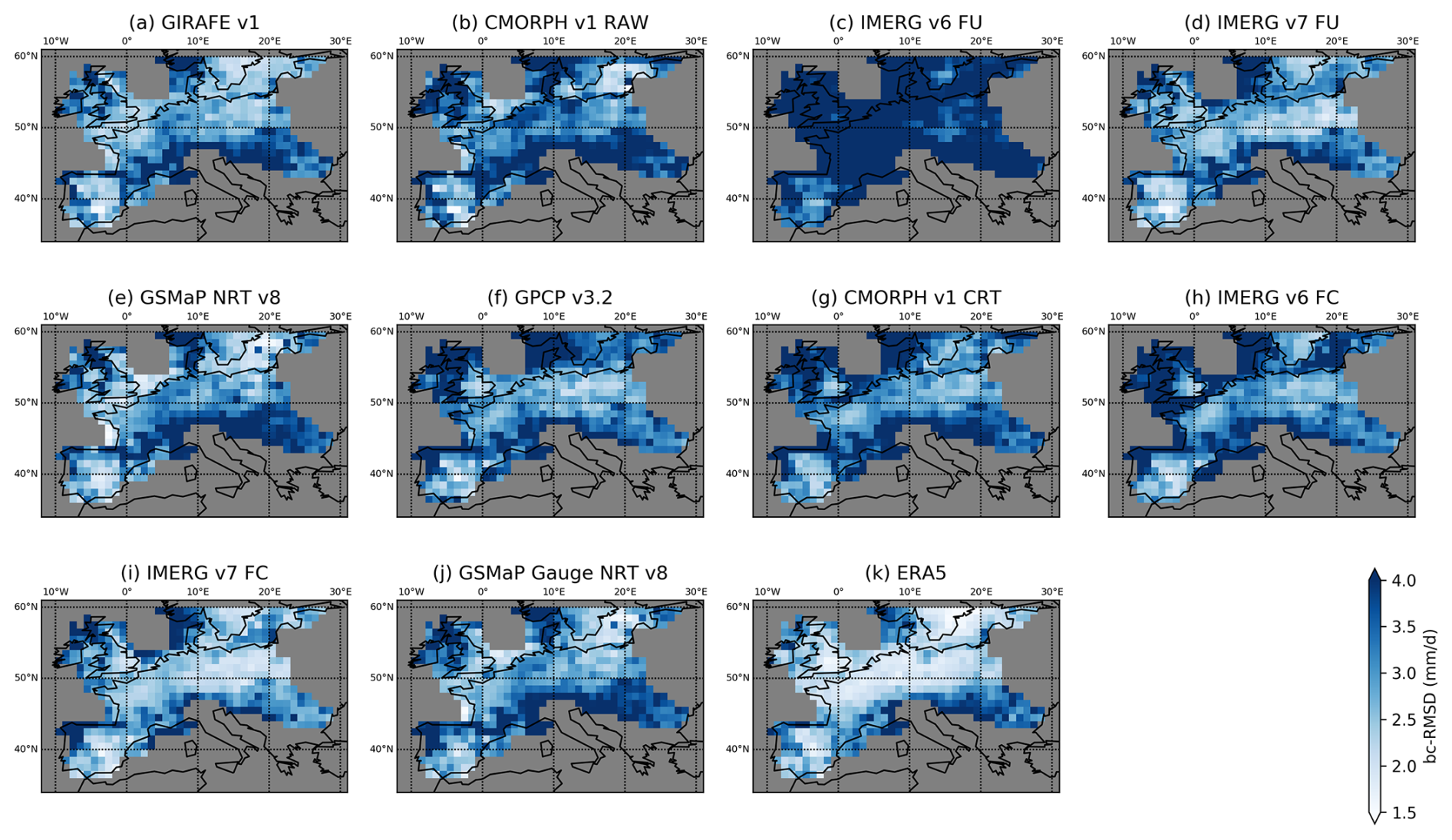
Figure 7Maps of the bc-RMSD in the 1DD precipitation for the validated datasets against EURADCLIM. The datasets appear in the same order as in Table 5. Panels (a–e) represent the unadjusted datasets, (f–j) represent the adjusted datasets, and panel (k) represents the ERA5 reanalysis. GIRAFE v1 has been analysed without the application of the snow flag. The analysis of CMORPH v1 RAW (panel b) ends in July 2017; all other comparisons extend over mutually available grid cells in the 2013–2020 period.
The detection statistics of GIRAFE v1 (and hence also CC) suffer from a relatively low POD (Table 5). Other unadjusted datasets have similarly low or lower POD, while the adjustment towards rain gauges for most datasets alleviates this effect. The evaluation of GIRAFE v1 over summer months only (row 2 in Table 5) yields a significant improvement in all measures towards or above the other datasets’ all-year performance, while the evaluation of GIRAFE v1 over the entire year, but with the SIF (Sect. 4.6) applied, ranges in between. Hence, the low POD is likely related to detecting snowfall or liquid/mixed precipitation over snow and ice-covered regions. It should be noted that the application of the SIF removes ∼45 % of the 1DD grid cells in the EURADCLIM-GIRAFE v1 comparison due to the conservative extension of the ERA5 information on snow and sea-ice cover to a 3DD environment (Sect. 4.6). Again, the adjusted datasets score better in principle than their unadjusted counterparts, indicating the potential of a future adjustment in GIRAFE. Finally, as in Sect. 5.1.1, in the absence of 1DD uncertainty estimates in the other datasets, GIRAFE v1 outperforms these in terms of FEBO; a more detailed discussion of the sampling uncertainty can be found in Sect. 5.6.
5.2 Intercomparison with (quasi-)global datasets
GIRAFE v1 features the expected climatological patterns over the globe (Fig. 8, panel a vs. b–g). It tends to overestimate precipitation with respect to the other datasets in the tropical rain belt and in the western Pacific Ocean (Fig. 8h), except in South America. At higher latitudes, GIRAFE v1 generally tends to underestimate the other datasets, with a few exceptions such as western North America or the North American Atlantic coast. This general underestimation is at least partially related to the inadequate detection of precipitation over snow and ice surfaces discussed in Sect. 5.1.2 and shows up strongest in the sub-polar Antarctic, where GIRAFE v1 misses most precipitation over sea ice. The different treatment of 1DD grid cells inside and outside of 55° N/S in GIRAFE v1 (Sect. 4.3) manifests in latitudinal discontinuities at the boundaries (Fig. 8a and g, also in Fig. 11).
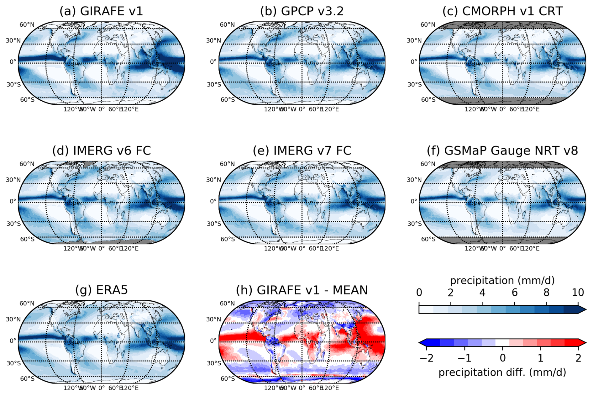
Figure 8Spatial distributions of climatological mean precipitation (2002–2020) for various datasets (a-g). Panel h: difference between the GIRAFE v1 climatological mean (panel a) and the ensemble mean of the other datasets (panels b–g).
As an example of GIRAFE v1's temporal evolution compared to these other datasets, we focus on low latitudes. Again, the validation report (Konrad et al., 2024) contains a more detailed picture for other regions, too. Over land, on average, GIRAFE v1 resembles the other datasets closely (Fig. 9a), except CMORPH v1 and GSMaP v8, which are biased low compared to the other datasets. Over low-latitude ocean (Fig. 9b), all datasets show a relation to ENSO, with precipitation being highest during El Niño events. GIRAFE v1 sees the highest precipitation in this region (see also the discussion of Fig. 8h above) and also the strongest link to ENSO. This is most likely inherited from the HOAPS PMW dataset, which has been shown to be more sensitive than others (Masunaga et al., 2019).
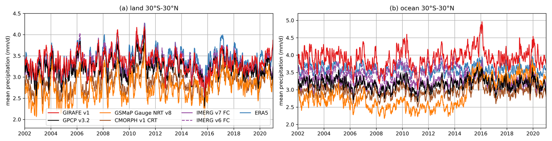
Figure 9Time series of mean precipitation inside 30° N/S separately for land (a) and ocean (b) for various datasets. The thick coloured lines are obtained via application of a 30 d running average.
Without a clear reference, the most obvious deviations of GIRAFE v1 from the other datasets over tropical oceans in terms of more precipitation and a stronger correlation with ENSO are currently classified as a feature rather than a deficiency.
5.3 Homogeneity analysis
Homogeneity is an important aspect in a dataset that is designed for climate applications, as inhomogeneities, or breakpoints, stemming from changes in the observing system can be misinterpreted as a climate signal. In this section, we assess the degree of homogeneity of GIRAFE v1 and other datasets in terms of the occurrence of breakpoints, following methods by Weatherhead et al. (1998) and Mieruch et al. (2014), also utilised in GEWEX water vapour assessment (Schröder et al., 2016, 2019; Trent et al., 2024). Various homogeneity tools exist (see Venema et al., 2012, for an overview). We apply two tests: the Penalised Maximal F (PMF) test (Wang, 2008a, b) and a variant of the standard normal homogeneity (SNH) test (Hawkins, 1977; Alexandersson, 1986), as proposed in Reeves et al. (2007). The SNH test is carried out only on breakpoints previously identified by the PMF test. The detection of a breakpoint confirmed by the SNH test can then be considered to be of increased confidence because of the 2-fold evaluation. These situations are referred to as “confirmed breakpoints” in the discussion below. The resulting breakpoint analysis detects abrupt changes in a time series of precipitation at a 0.05 significance level, in terms of the timing and the strength of the breakpoint.
Input to the PMF and SNH tests are time series of anomaly differences, i.e. the difference between the anomalies from a dataset and a reference dataset after removal of the mean annual cycles. Using a record as reference does not constitute a statement on superior quality. Instead, references are chosen because they are widely used, have global (land) coverage, and are observation-based (GPCP v3.2, GPCC v2022) or are independent from the former datasets (3B42 v7 after 2000, CMORPH V1 CRT, which uses the rain-gauge-based dataset CPC; Chen et al., 2008). For each region and analysed parameter (rows in Fig. 10), two reference datasets are chosen to further increase confidence in breakpoints (columns in Fig. 10): the occurrence of simultaneous breaks against both reference datasets points to a homogeneity issue in the dataset under consideration. Conversely, mutual breakpoints in several datasets against the same reference dataset may indicate an inhomogeneity in the respective reference dataset.
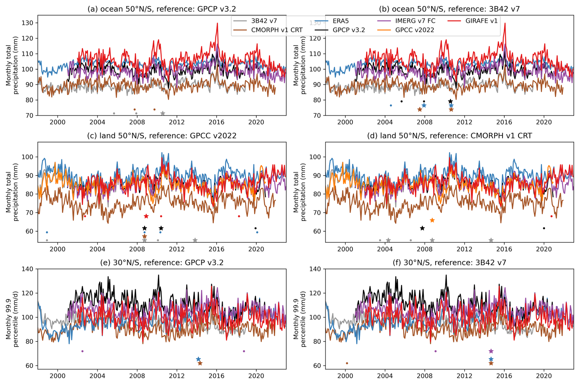
Figure 10Homogeneity analysis. (a) Monthly total precipitation over ocean inside 50° N/S with GPCP v3.2 as the reference dataset for the homogeneity tests. (b) Same but with 3B42 v7 as the reference dataset. (c) Monthly total precipitation over land inside 50° N/S with GPCC v2022 as the reference dataset for the homogeneity test. (d) Same but with CMORPH v1 CRT as the reference dataset. (e) 99.9th percentile of precipitation over land and ocean inside 30° N/S with GPCP v3.2 as the reference dataset for the homogeneity test. (f) Same but with 3B42 v7 as the reference dataset. The time series (identical in the left and right columns per row) illustrate the anomaly in the respective dataset shifted by the respective overall mean. Small, circle-shaped markers indicate the presence of breakpoints detected by the PMF test only. Breakpoints, illustrated by large, star-shaped markers, are also confirmed by the SNH test. A complete list of detected breakpoints is given in Appendix C. Note that some time series start between January 1998 and January 2002 or end prior to December 2022, deviating from the GIRAFE v1 coverage.
The anomaly differences analysed in these tests are based either on monthly totals (Fig. 10a–d) or – representing extreme precipitation (see also Sect. 5.5) – on the monthly 99.9th percentile (Fig. 10e and f), each transferred to log-scale and each based on the 1DD GIRAFE v1 product and FROGS variants of the other datasets. If a grid-based time series of daily accumulated precipitation does not cover all days, the monthly total based on the available daily values is scaled accordingly. More sophisticated approaches use, for example, reference climatologies (Wang et al., 2023). Finally, it is noted that the breakpoint analysis is affected by uncertainties; in particular, actually existing breakpoints might go undetected.
Figure 10 shows the anomaly time series and associated breakpoints in the various settings for GIRAFE v1 and several of the previously introduced datasets. For a detailed overview, Appendix C provides a list of all breakpoints shown in the various panels. Here, we focus on the discussion of the homogeneity of GIRAFE v1; however, some implications of breakpoints in the other datasets are discussed in Sect. 5.4. Over global ocean surfaces inside 50° N/S, GIRAFE v1 does not exhibit confirmed breakpoints (no red star-shaped markers in panels a and b of Fig. 10), while over land inside 50° N/S, a single, confirmed breakpoint is detected in December 2008. This breakpoint is only present relative to GPCC v2022 but not relative to CMORPH v1 CRT (red star-shaped marker in panel c but not in panel d). This reduces confidence in the presence of a breakpoint in GIRAFE v1 and points to a potential issue in GPCC v2022, which is generated from various input streams of rain gauge data and intense and – to a significant extent – manual quality control. The combination of this leads to a delay in the ingestion of data and causes a strong, abrupt decrease in the amount of input data in approximately 2009 (see Fig. 1 in Schneider et al., 2022), coinciding with the observed break in GIRAFE v1 and those of other datasets against GPCC v2022 in October 2008 (GPCP v3.2 and ERA5; see also the full list of breakpoints in Appendix C). Note that, consistent with this, GPCC v2022 together with 3B42 v7 exhibits a breakpoint relative to CMORPH v1 in October 2008 (again, see also Appendix C). Further analysis is needed to better understand this feature. GIRAFE v1 does not exhibit confirmed breakpoints relative to GPCP v3.2 and 3B42 v7 in terms of the monthly 99.9th percentile inside 30° N/S (no red star-shaped marker in panels e and f), and it is therefore concluded that GIRAFE v1 proves stable in terms of extremes.
5.4 Stability analysis
Breakpoints, as discussed in Sect. 5.3 or, artificial trends caused by drifts or ageing of the observing system itself rather than the Earth system affect the stability of a CDR. Again following Weatherhead et al. (1998), Mieruch et al. (2014), Schröder et al. (2016, 2019), and Trent et al. (2024), we define stability as the trend in a time series of the bias of one dataset relative to another one over a given spatial area and assess the stability of GIRAFE v1 in this sense. Trends in the single datasets were computed as well, utilising the same methods, but applied to absolute values rather than differences (bias). A linear trend model, the amplitudes and frequencies of four modes, and the strength of ENSO were simultaneously fitted to the time series analysed in Sect. 5.3. The uncertainty of the linear trend estimates was corrected for autocorrelation of autoregressive data of order 1 (Schröder et al., 2019). The significance of the stability being different from 0 at a level of 0.05 was assessed as well. The trends and the stability were estimated for the same cases as in the homogeneity analysis (Sect. 5.3; monthly totals inside 50° N/S separately for ocean and land and the 99.9th percentile inside 30° N/S). Results are shown in Table 6.
Table 6Trends (i.e. in time series of absolute values in single datasets) in the various datasets (left block) and stabilities of GIRAFE v1 against the respective reference dataset (i.e. trends in time series of differences; right block) and their uncertainty in in the 2002–2020 period. Asterisks (*) indicate significant trends/stabilities.
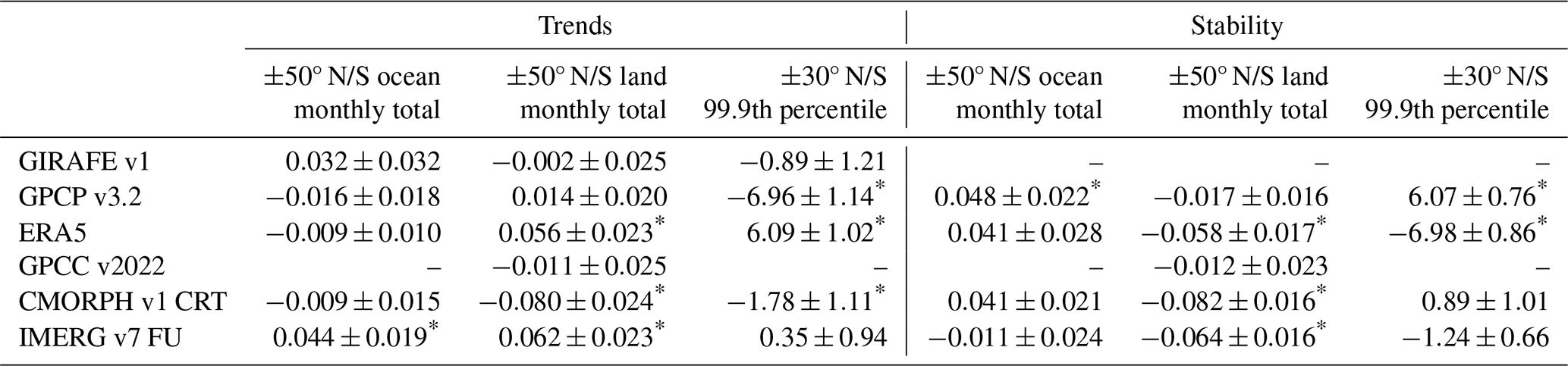
In general, an increase in precipitation with an increase in surface temperature is expected, which – in a warming climate – would manifest as a positive trend over time. In particular, over the ocean, such an increase is to be expected, as the supply of water vapour via evaporation feeding precipitation is not limited. Over land, such an increase might be subdued, as the supply of water vapour through evapotranspiration and advection is limited (e.g. Roca, 2019a). In our analysis, trends are not significant in the majority of cases. In particular, GIRAFE v1 exhibits no significant trend in the considered settings. However, the considered period is relatively short, and, even on these spatially aggregated scales, quite a significant level of variability exists. Both factors impact the significance of trend estimations.
The stability estimates in Table 6 (right block) are all given between GIRAFE v1 and the various listed datasets. GIRAFE v1 is stable with respect to a given dataset if the respective stability value does not deviate significantly from 0 . In general, the stability estimates do not exhibit a unique pattern in terms of significance. GIRAFE v1 exhibits negative stabilities over land relative to all other considered datasets. However, the smallest and also non-significant stability occurs relative to GPCC (). Over ocean, where, in general, a positive trend is expected (see above), GIRAFE v1 shows a non-significant positive trend in contrast to the non-significant negative trend of GPCP v3.2 (left block in Table 6). This discrepancy in the trends explains the significantly non-zero stability estimate (0.048 ) between the two.
The largest and second largest stability values of GIRAFE v1 for extremes (99.9th percentile, ±30° N/S columns in Table 6) are observed relative to ERA5 and GPCP v3.2, respectively, with opposite signs. We note that GIRAFE v1 does not show confirmed breakpoints (Sect. 5.3) and generally shows a non-significant and smaller trend in the 99.9th percentile (left block in Table 6). The opposite signs in stability of GIRAFE v1 against these two datasets is thereby caused by the decreasing trend in GPCP v3.2 and an increasing trend in ERA5 in extremes, as evident in Table 6 (left block) and Fig. 10e and f. Again, we can argue with expectations, i.e. with increasing surface temperatures, the extremes in precipitation are expected to increase and not decrease (see also Sect. 5.5). However, the results are based on land and ocean observations, with land potentially undergoing an unknown moisture supply. When looking closer at Fig. 10e and f, extremes in GPCP v3.2 and ERA5 agree well after 2014, but in the early part of the period, both exhibit maximum difference. This approximately coincides with the end of the TRMM/TMI data in 2014/2015. Given that both datasets exhibit the largest negative and positive trends, this can be an indication that both are affected by stability issues. At the same time, CMORPH v1 CRT, ERA5, and IMERG v7 FU might also be affected by breakpoints relative to GPCP v3.2 and 3B42 v7 (Fig. 10e, f and Appendix C), possibly also caused by the removal of TRMM/TMI in these reference datasets. Sound conclusions regarding a potential stability issue in GPCP v3.2 and ERA5 are not possible, and further analysis is needed. A potential way forward can be to follow the approaches outlined in Nguyen et al. (2024), replacing the use of data from neighbouring stations in this study with that of multiple datasets.
We conclude here that GIRAFE v1 has stability well within the range of available, widely used precipitation datasets, both in terms of the monthly total (i.e. mean) and extreme precipitation.
5.5 Scaling of daily precipitation extremes with surface temperature
5.5.1 Qualitative analysis
Daily extreme precipitation is conventionally defined with the high percentile of the daily wet-days precipitation distribution (Schär et al., 2016). Figure 11 shows the map of the climatology of the annual 99.9th percentile based on the GIRAFE v1 data and allows for a discussion of the representation of extreme precipitation in GIRAFE v1 in the following. It is very similar to Rx1d maps (Bador et al., 2020; Alexander et al., 2020), although magnitudes vary across extreme indicators Rx1d and the 99.9th percentile as well as across datasets. As expected, it further resembles the climatology of large and organised convective systems (Roca and Fiolleau, 2020), with well characterised maxima in the North America Great Plains and in South America over Argentina. Orographic features can also be easily spotted. Over ocean, the map recalls the link between intense extremes and hurricanes as exemplified by the local maximum in the Philippines Sea, Bay of Bengal, and Eastern Pacific. The boundary for the inclusion or exclusion of infrared observations from geostationary satellites at 55° S shows in the Southern Ocean; see also Fig. 8 and the related discussions in Sect. 5.2. Regions poleward of 55° N/S, where the absence of geostationary IR observations and the deficiencies of the PMW-derived precipitation rate estimates (cf. Sect. 5.1.2) prevent a correct estimation of the extremes, are likely not well represented in GIRAFE v1, particularly in the Southern Hemisphere. Beyond this well-identified problem, the overall consistency of this diagnostic gives confidence in the ability of GIRAFE v1 to characterise the geographical distribution of extreme precipitation.
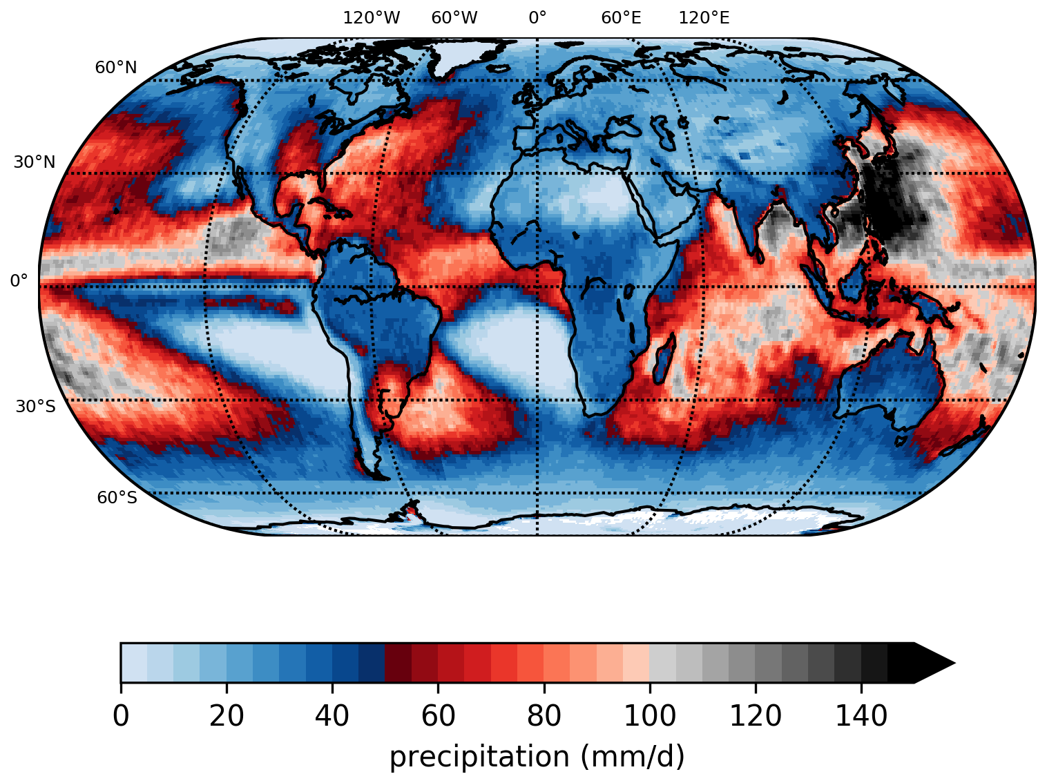
Figure 11Map of the 2002–2020 multi-year mean of the annual 99.9th percentile of GIRAFE v1 daily precipitation (mm d−1).
5.5.2 Quantitative analysis
Over the tropical ocean, precipitation is tightly linked to low-level moisture. In the case of extreme precipitation, it is possible to further quantify this sensitivity by using SST as a proxy for moisture and simple scaling arguments (Muller and Takayabu, 2020). Based on these theoretical considerations, an increase in the extreme is expected with SST at a rate of following the Clausius–Clapeyron equation. De Meyer and Roca (2021) used the OSTIA SST (Good et al., 2020) and a data pooling technique to estimate this scaling from the observed record. This method has been replicated here. For each SST bin of 0.5 K, all the corresponding wet-days () precipitation are pooled together. Note that the SST values are lagged by 48 h to remove the cooling effect of the precipitation onto the SST (De Meyer and Roca, 2021). A 5-year period of randomly selected individual, i.e. not necessarily consecutive, years within the 2007–2020 period is used for the data pooling, and the 99.9th percentile is estimated from this distribution. Furthermore, a bootstrap of 50 members is constructed using this method. The mean and standard deviation of the 50-member ensemble 99.9th percentile are finally computed.
Figure 12 shows the resulting sensitivity of the 99.9th percentile to the SST for GIRAFE v1 and other products used above for comparison. Between 300.25 and 302.25 K, where 60 %–80 % of the data points fall, all the products exhibit a linear regime, in agreement with previous studies (De Meyer and Roca, 2021). Over this “Clausius–Clapeyron” regime, extreme precipitation ranges from 120 to 170 mm d−1, highlighting the difference in magnitude among the products, which is smaller than that of a previous assessment based on older products (Roca et al., 2021). GIRAFE v1 stands in the middle, with the CMORPH v1 product being systematically lower and the GPCP v3.2 and IMERG v7 products being larger. As far as the scaling (the slope of the linear regime) is concerned, the products show better agreement than for the ensemble mean estimate of the 99.9th percentile. The scaling is for GPCP v3.2, for GIRAFE v1, for CMORPH v1, and for IMERG v7, in good agreement with the Clausius–Clapeyron rate. The small variance of the estimate when bootstrapped over the 14-year period () indicates a weak sensitivity to the selection of years, which in turn implies a weak sensitivity to the configuration of the microwave constellation used in these products, in agreement with data-denial experiments (Jucá Oliveira et al., 2022). A discussion of the overall divergence of the datasets at SST<301 K, in which GIRAFE v1 appears exceptional, can be found in De Meyer and Roca (2021).
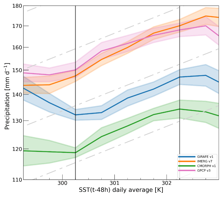
Figure 12The 99.9th percentile of the daily distribution as a function of the 48 h-lagged underlying SST for several products, including GIRAFE v1. The lines correspond to the 50-member ensemble mean, and the shading represents the standard deviation. The vertical lines delineate the central section of the distributions, representing the majority of the data (see main text).
These diagnostics of extreme precipitation consolidate the compliancy of GIRAFE v1 with climate science and monitoring objectives.
5.6 Plausibility of the sampling uncertainty
In this section, the plausibility and usability of the GIRAFE v1 sampling uncertainty is discussed in terms of (i) its agreement with reference datasets within the given uncertainties (“consistency”) and (ii) its overall distribution and general asymptotic behaviour. The consistency with reference datasets has been briefly covered in the validation against AMMA-CATCH and EURADCLIM (Sect. 5.1). In general, the FEBO of GIRAFE v1 and hence the consistency is larger than that of other 1DD datasets, as these do not feature 1DD uncertainty estimates; hence, they can only agree with the reference datasets within the uncertainties of the latter and not the mutual uncertainty as in the case of GIRAFE v1. Figure 13 shows the positive correlation of the GIRAFE v1 sampling uncertainty and the absolute difference in collocated GIRAFE v1 and EURADCLIM 1DD (Sect. 5.1.2). The sampling uncertainty can hence, in principle, be used as a proxy for the mismatch of GIRAFE v1 from ground-based reference observations. However, the relatively low overall level of the GIRAFE v1 FEBO (60 % against AMMA-CATCH and EURADCLIM in summer months; see Sect. 5.1) and the prevalence of GIRAFE v1/EURADCLIM differences exceeding the GIRAFE v1 uncertainty (tilt towards the x axis in Fig. 13) indicate that the sampling uncertainty represents less than one sigma on average, i.e. underestimates the full GIRAFE uncertainty. However, systematic shifts in the detection of precipitation and related biases exist in the comparisons against both AMMA-CATCH and EURADCLIM (high FAR coinciding with positive bias against AMMA-CATCH (Sect. 5.1.1) and low POD coinciding with negative bias against EURADCLIM (Sect. 5.1.2)). The underlying retrieval uncertainties cannot be covered by the GIRAFE v1 sampling uncertainty and explain at least parts of its above-mentioned shortcomings.
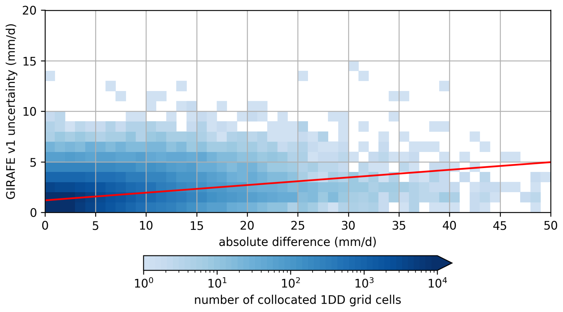
Figure 13Two-dimensional distribution (colour-coded) of absolute deviations between collocated 1DD GIRAFE v1 and EURADCLIM data (x axis) and the magnitude of the GIRAFE v1 sampling uncertainty (y axis). Here, the data in 1DD grid cells identified as snow-covered (Sects. 4.6 and 5.1.2) and with GIRAFE v1 daily precipitation of less than 1 mm have been discarded, i.e. the effect of missed precipitation in GIRAFE v1 (Sect. 5.1.2) is suppressed here. The red line shows the linear least-squares fit to the collocated data points that underlie the distribution, indicating a positive correlation.
The overall distribution and asymptotic behaviour of the GIRAFE v1 sampling uncertainties are verified against TAPEER v1.5 sampling uncertainties. The GIRAFE v1 uncertainties are modelled after those of TAPEER, but the underlying PMW databases differ between GIRAFE v1 and TAPEER v1.5, so the values should not be expected to be identical. Figure 14 shows the occurrence of 1DD data points along the dimensions of the relative uncertainties in GIRAFE v1 and TAPEER and of daily precipitation. GIRAFE v1 shares the asymptotic behaviour of TAPEER v1.5 for high 1DD precipitation values. In general, GIRAFE v1 has narrower distributions along the precipitation dimension (x axis), especially over ocean. This likely stems from a general tendency of GIRAFE v1 towards fewer occurrences of high precipitation in GIRAFE v1, as documented by Konrad et al. (2024). With TAPEER sampling uncertainties extensively studied and validated against ground-based datasets (Chambon et al., 2013; Gosset et al., 2018), the overall agreement of GIRAFE v1 with TAPEER v1.5 underlines the plausibility of the GIRAFE v1 sampling uncertainties.
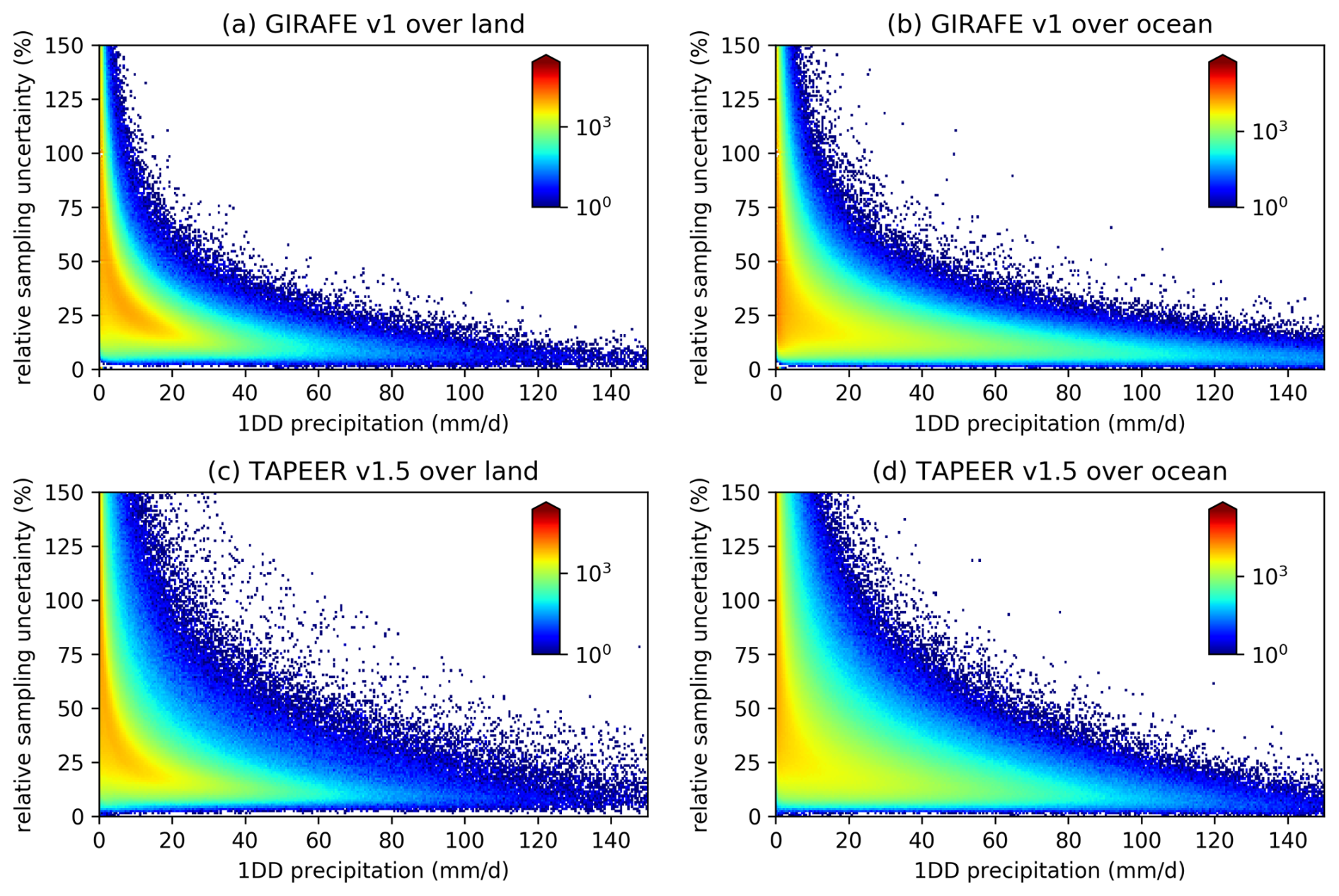
Figure 14Two-dimensional histograms of the 1DD relative sampling uncertainties and the 1DD precipitation in GIRAFE v1 (a, b) and TAPEER v1.5 (c, d) from all 1DD grid cells in 2012–2021 inside 30° N/S (TAPEER v1.5 coverage), for which the decorrelation scales were not replaced by default values in GIRAFE v1 (see Sect. 4.4), separately for land (a, c) and ocean (b, d).
The data record DOI for GIRAFE v1 is https://doi.org/10.5676/EUM_SAF_CM/GIRAFE/V001 (Niedorf et al., 2024a). Data and associated documentation (scientific references, algorithm theoretical basis documents, validation reports, and user manuals) are available at the above dataset URL.
All intellectual property rights of the CM SAF GIRAFE v1 products belong to EUMETSAT. The use of these products is granted to every interested user, free of charge. If you wish to use these products, EUMETSAT's copyright credit must be shown by displaying the words “copyright (year) EUMETSAT” on each of the products used.
As explained in Sect. 4.3, unofficial variants of the GIRAFE v1 datasets with different start times for 1 d (06:00, 12:00, 18:00 UTC) exist and can be acquired through the CM SAF user help desk. Likewise, CM SAF retains the decorrelation scales (Sect. 4.4) as unofficial output for interested expert users.
Feedback on GIRAFE v1 is appreciated by the authors and can be submitted via the CM SAF user help desk.
PMW imager observations are used as input to the HOAPS retrieval (Sect. 3.2.1). For instruments SSM/I and SSMIS, the CM SAF SSMI(S) FCDR is available at https://doi.org/10.5676/EUM_SAF_CM/FCDR_MWI/V004 (Fennig et al., 2022). Level-1 observations by TMI, AMSR-E and GMI are downloaded from https://disc.gsfc.nasa.gov/datacollection/TRMM_1B11_7.html (TRMM, 2011), https://doi.org/10.5067/GPM/AMSRE/AQUA/1/07 (Berg, 2021), and https://doi.org/10.5067/GPM/GMI/GPM/1B/07 (GPM Science Team, 2022) and intercalibrated with and intercalibrated with the SSMI(S) FCDR as described by Fennig (2022).
PMW sounder observations are used as input to the PNPR-CLIM and PRPS retrievals (Sects. 3.2.2 and 3.2.1). Observations by the instruments AMSU-B and MHS from 2002–2017 are available from the FIDUCEO archive at https://doi.org.10.5285/a8e9f44965434f3b861eba 77688701ef (Hans et al., 2020). MHS Level-1 data from 2018 onwards are downloaded from the NASA PPS archive at the following sources: https://doi.org/10.5067/GPM/MHS/METOPA/1C/07 (Berg, 2022a), https://doi.org/10.5067/GPM/MHS/METOPB/1C/07 (Berg, 2022b), https://doi.org.10.5067/GPM/MHS/ METOPC/1C/07 (Berg, 2022c), https://doi.org.10.5067/GPM/MHS/ NOAA18/1C/07 (Berg, 2022d), and https://doi.org.10.5067/GPM/MHS/ NOAA19/1C/07 (Berg, 2022e). ATMS Level-1 data are downloaded from the NASA PPS archive at https://doi.org/10.5067/GPM/ATMS/NOAA20/1C/07 (Berg, 2022f) and https://doi.org/10.5067/GPM/ATMS/NPP/1C/07 (Berg, 2022g). The precipitation rates obtained from SAPHIR observations by the PRPS retrieval are available at https://doi.org/10.5067/GPM/SAPHIR/MT1/PRPS/2A/06 (Kidd, 2019).
ERA5 data as ancillary input to PNPR-CLIM (Sect. 3.2.2) and for constructing the SIF (Sect. 4.6) are available at https://doi.org/10.24381/cds.f17050d7 (Hersbach et al., 2023). Sea-ice, lake-ice, and SST information from the OSTIA product is available at https://doi.org/10.48670/moi-00168 (Marine Data Store, 2025).
MEI v2 data used in the construction of the quantile mapping (Sect. 4.2) have been downloaded from https://psl.noaa.gov/enso/mei/ (NOAA, 2025).
The precipitation datasets used for the quality assessment in Sect. 5 are taken from https://doi.org/10.14768/06337394-73A9-407C-9997-0E380DAC5598 (Roca et al., 2019b). Exceptions are EURADCLIM (accessible through https://doi.org/10.21944/1a54-gg96, Overeem et al., 2022) and AMMA-CATCH (Lebel et al., 2009).
GIRAFE v1 is a new satellite-based CDR for precipitation, available globally on 1DD and 1DM regular grids from 2002 to 2022. The implementation and generation were carried out by CM SAF in response to the outcome of a dedicated workshop series. The methods for merging PMW and IR observations as presented in Sect. 4.3 are based on TAPEER (Chambon et al., 2013). The derivation of precipitation rate estimates from PMW observations (Sect. 3.2) is based on various previous works (Andersson et al., 2010; Bagaglini et al., 2021; Kidd et al., 2021).
In terms of product content, GIRAFE v1 stands out with a dedicated and plausible sampling uncertainty, allowing a more robust quantitative analysis of precipitation at 1DD scale. In terms of quality, GIRAFE v1 is able to reproduce reference datasets similar to previously existing products, especially to those that are like GIRAFE v1 not adjusted to ground-based data (Sects. 5.1 and 5.2). Among the (quasi-)global products, GIRAFE v1 stands out in terms of homogeneity (Sect. 5.3) and stability (Sect. 5.4), at least partially in response to the dedicated post-processing of PMW-based precipitation rate estimates (Sect. 4.2). GIRAFE v1's usefulness for analysing extreme precipitation has been shown in Sect. 5.5. Overall, these analyses underline the compliancy of GIRAFE v1 with requirements for usage in climate monitoring and climate sciences.
The primary uses of GIRAFE v1 include climate monitoring, climate analysis and services, water cycle research, and climate model evaluation. It is valuable to a wide range of users, including hydrometeorological services, research institutions, universities, civil and environmental protection agencies, insurance and reinsurance companies, United Nations agencies, water management authorities, agriculture and food production ministries, and transportation companies and authorities. These needs align with the WMO Global Framework for Climate Services (GFCS) priority areas, which include agriculture and food security, disaster risk reduction, health, and water availability.
The most apparent limitation of GIRAFE v1 is the low POD of precipitation in mid-to-high latitudes in the presence of surface snow or ice, inherited from the PMW-based precipitation estimates (Sects. 5.1 and 5.2). Interpretations of GIRAFE v1 data in these situations should be carried out carefully. A respective quality flag allows users to identify potentially affected grid cells. Another limitation is the high fraction of false precipitation during the rainy season in West Africa (Sect. 5.1).
The number of available 1DD grid cells varies over time, due to the constellation of PMW sensors in orbit, with more gaps occurring at the start of the GIRAFE v1 time series. The stability of the dataset is affected only to a small degree by the lower amount of PMW-based observations (see Sects. 5.3 and 5.4 and the results by Jucá Oliveira et al., 2022).
CM SAF provides a framework for the continuous development and operation of CDRs. Hence, the GIRAFE efforts will continue, with an interim CDR (ICDR) that continues the GIRAFE v1 time series from 2023 onwards. CM SAF aims to operationally produce the GIRAFE v1 ICDR in 2025. Subsequently, efforts will be dedicated to developments towards an improved new version. The latter will address the above-mentioned limitations of GIRAFE v1, the enhancement of uncertainty estimation in addition to the infrared-based sampling uncertainty, a redefinition of the areas in which GIRAFE works in different ways (currently inside and outside 55° N/S; see Sect. 4.3) and their associated settings (thresholds, extent of local environments), and – using data from qualified sensors – the extension forward and backward in time. Wherever possible, the prioritisation of improvements will be carried out in close coordination with users during regular workshops. Interested readers are invited to contact CM SAF.
Here, we show the positive effect of the quantile mapping procedure described in Sect. 4.2 on the final GIRAFE output, exemplarily in the case of the precipitation rate estimates by Megha-Tropiques SAPHIR PRPS (MT from here). The original MT distribution sees more rates below 0.5 mm h−1 than the distribution of the target satellite METOP-A MHS PNPR-CLIM (Fig. A1a; blue vs. black line). The unadjusted MT observations in the PMW input stream introduce a strong negative bias output compared to GIRAFE output without MT observations ingested (Fig. A1b) because the lower ratio of MT observations exceeding the GIRAFE detection threshold of 0.5 mm h−1 implies fewer precipitation events are detected in the IR observations (Sect. 4.3.1). MT observations are available only from 2012 to 2020, so this situation leads to a temporal instability (discontinuity) when MT enters and leaves the constellation. Quantile mapping brings the MT distribution very close to the target (Fig. A1a; red vs. black line) from rates of about 0.3 mm h−1, i.e. the distributions are aligned at the detection threshold of 0.5 mm h−1. The inclusion of the mapped MT data in GIRAFE causes much smaller deviations from the variant not using MT data than without quantile mapping (Fig. A1c), and the structural negative bias introduced by MT is mostly remedied. Differences remain that might be linked to deviations in the diurnal sampling between MT and the target satellite or non-representativity of the distributions towards the boundaries of the latitude/longitude bands.
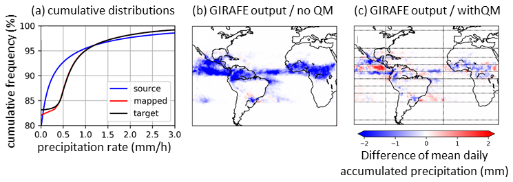
Figure A1(a) Exemplary cumulative distributions for METOP-A MHS PNPR-CLIM (“target”; black) and Megha-Tropiques SAPHIR PRPS (MT from here; “source”; blue) from instantaneous observations in June at latitudes inside 4° N/S over South American land. The MT distribution after quantile mapping has been applied (“mapped”; red) is also shown. (b) Differences in GIRAFE daily accumulated precipitation with and without MT instantaneous data averaged over June 2014. Here, quantile mapping has not been applied. (c) Same as (b) but with quantile mapping applied. The lines delineate the latitude/longitude bands in which the cumulative distributions are collected. Note that the results in (b) and (c) depend not only on the data forming the distributions shown in (a) but also on those in the other latitude/longitude bands, depending on the location.
Figure B1 illustrates the mutual availability of the datasets in the comparison against EURADCLIM discussed in Sect. 5.1.2. The comparison of CMORPH v1 RAW against EURADCLIM is based on fewer grid cells because this dataset ends in 2017. The comparison against GIRAFE v1 during summer months and when filtering out SIF-flagged 1DD grid cells is also based on fewer grid cells due to this filtering. Zero availability, as illustrated by the grey areas in Fig. B1, is mostly caused by the geographical restrictions in the EURADCLIM dataset, except at the 60° N boundary, where some of the quasi-global datasets are limited.
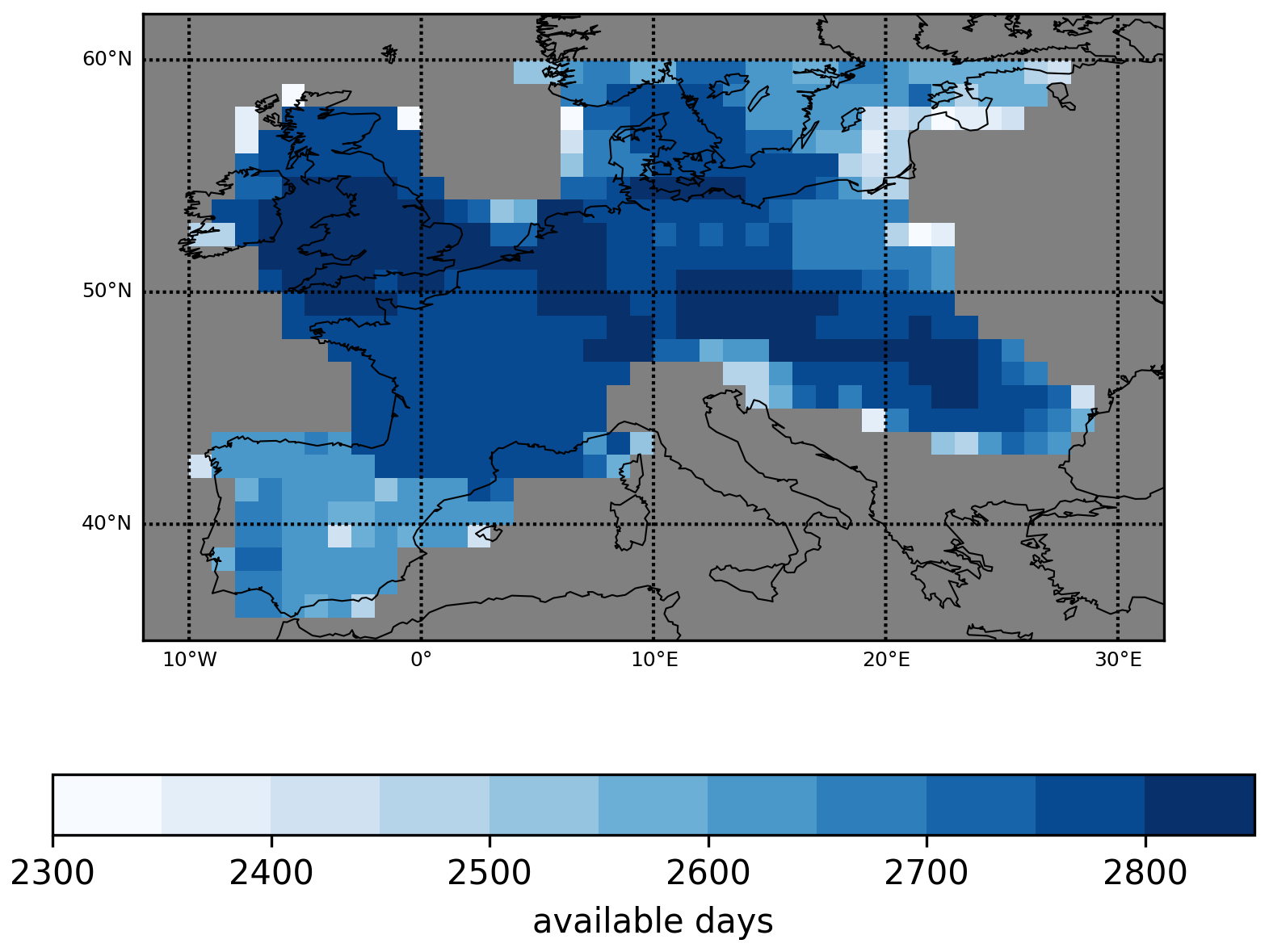
Figure B1Number of days during the 2013–2020 period for which 1DD grid cells are available over Europe in the comparison of 1DD datasets against the ground-based radar dataset EURADCLIM. Grey indicates zero availability.
Table C1 lists the breakpoints discussed in Sects. 5.3 and 5.4 for the respective settings and reference datasets. Note that some breakpoints occur in times preceding the GIRAFE v1 CDR (2002).
Table C1Breakpoints at monthly resolution detected by the PMF test, as shown by the vertical lines in Fig. 10 and discussed in Sects. 5.3 and 5.4. NA: not available because dataset is a respective reference dataset. Asterisks (*) indicate breakpoints that are confirmed by the SNH test (bold vertical lines in Fig. 10).
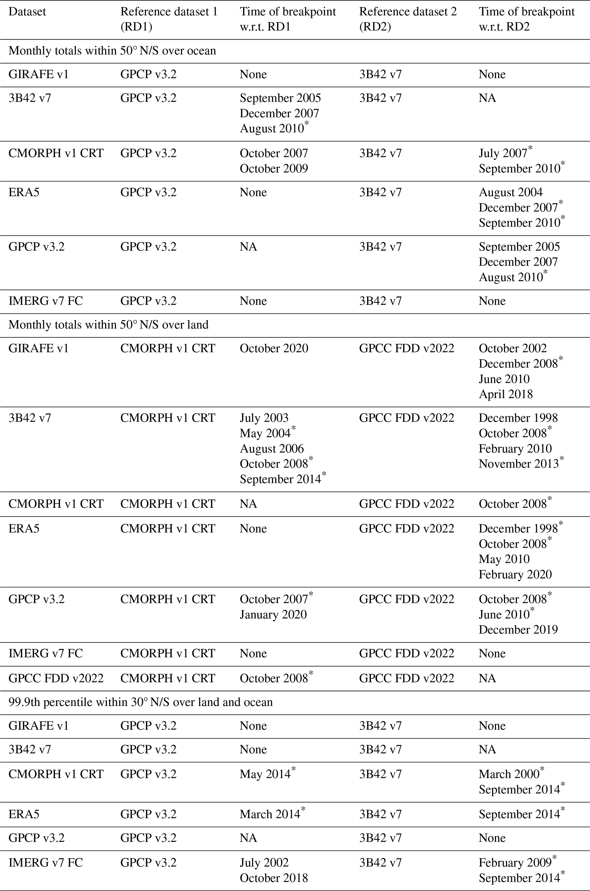
HK prepared the original manuscript with substantial contributions from RR, MS, SF, and AN. SF built the archive of geostationary infrared observations. TS and SF implemented the infrared quality control under the guidance of SC. AN, TS, KF, and HK built the PMW archive. GP, PS, CK, and KF developed the PMW precipitation retrievals and advised on the PMW archive. HK implemented the PMW pre-processing. SF and AN implemented the merging and sampling uncertainty algorithms under the guidance of RR, SC, and RAJO. HK, MS, RR, and ML carried out the analyses in Sect. 5. All authors contributed to the revision of the original manuscript.
The contact author has declared that none of the authors has any competing interests.
Publisher's note: Copernicus Publications remains neutral with regard to jurisdictional claims made in the text, published maps, institutional affiliations, or any other geographical representation in this paper. While Copernicus Publications makes every effort to include appropriate place names, the final responsibility lies with the authors.
The PNPR-CLIM algorithm was developed by CNR-ISAC in the C3S_312b_Lot 1 Copernicus Climate Change Service project, for which a licence agreement exists between DWD and CNR-ISAC. This study benefited from the IPSL mesocenter ESPRI facility, which is supported by CNRS, UPMC, Labex L-IPSL, CNES, and Ecole Polytechnique. The authors thank Leonardo Bagaglini for his contribution in the development of PNPR-CLIM and Adrien Guérou, Marloes Penning de Vries, Ana Radovan, Felix Dietzsch, and Marc Pondrom for their contributions to the GIRAFE development at an early stage.
This work was performed within the EUMETSAT CM SAF framework, and the authors received financial support from the EUMETSAT member states. The European Union through the ECMWF Copernicus Climate Change Service (C3S) project C3S_312b_Lot1 “Copernicus Climate Change Service: Essential Climate Variable (ECV) products derived from observations Lot 1: precipitation, surface radiation budget, water vapour, cloud properties, and Earth radiation budget” supported the development of PNPR-CLIM.
This paper was edited by Qingxiang Li and reviewed by three anonymous referees.
A lexander, L. V., Bador, M. Roca, R., Contractor, S. Donat, M. G., and Nguyen, P. L.: Intercomparison of Annual Precipitation Indices and Extremes over Global Land Areas from in Situ, Space-Based and Reanalysis Products, Environ. Res. Lett., 15, 055002, https://doi.org/10.1088/1748-9326/ab79e2, 2020.
Alexandersson, H.: A homogeneity test applied to precipitation data, J. Climatol., 6, 661–675, https://doi.org/10.1002/joc.3370060607, 1986.
Andersson, A., Fennig, K., Klepp, C., Bakan, S., Graßl, H., and Schulz, J.: The Hamburg Ocean Atmosphere Parameters and Fluxes from Satellite Data – HOAPS-3, Earth Syst. Sci. Data, 2, 215–234, https://doi.org/10.5194/essd-2-215-2010, 2010.
Arkin, P. A.: The Relationship between Fractional Coverage of High Cloud and Rainfall Accumulations during GATE over the B-Scale Array, Mon. Weather Rev., 107, 1382–1387, https://doi.org/10.1175/1520-0493(1979)107<1382:TRBFCO>2.0.CO;2, 1979.
Bador, M., Alexander, L. V., Contractor, S., and Roca, R.: Diverse Estimates of Annual Maxima Daily Precipitation in 22 State-of-the-Art Quasi-Global Land Observation Datasets, Environ. Res. Lett., 15, 035005, https://doi.org/10.1088/1748-9326/ab6a22, 2020.
Bagaglini, L., Sanò, P., Casella, D., Cattani, E., and Panegrossi, G.: The Passive Microwave Neural Network Precipitation Retrieval Algorithm for Climate Applications (PNPR-CLIM): Design and Verification, Remote Sens., 13, 1701, https://doi.org/10.3390/rs13091701, 2021.
Berg, W.: GPM AMSR-E on AQUA Common Calibrated Brightness Temperatures L1C 1.5 hours 10.5 km V07, Greenbelt, MD, USA, Goddard Earth Sciences Data and Information Services Center (GES DISC) [data set], https://doi.org/10.5067/GPM/AMSRE/AQUA/1/07, 2021.
Berg, W.: GPM MHS on METOP-A Common Calibrated Brightness Temperature L1C 1.5 hours 17 km V07, Greenbelt, MD, Goddard Earth Sciences Data and Information Services Center (GES DISC), https://doi.org/10.5067/GPM/MHS/METOPA/1C/07, 2022a.
Berg, W.: GPM MHS on METOP-B Common Calibrated Brightness Temperature L1C 1.5 hours 17 km V07, Greenbelt, MD, Goddard Earth Sciences Data and Information Services Center (GES DISC) [data set], https://doi.org/10.5067/GPM/MHS/METOPB/1C/07, 2022b.
Berg, W.: GPM MHS on METOP-C Common Calibrated Brightness Temperature L1C 1.5 hours 17 km V07, Greenbelt, MD, Goddard Earth Sciences Data and Information Services Center (GES DISC) [data set], https://doi.org/10.5067/GPM/MHS/METOPC/1C/07, 2022c.
Berg, W.: GPM MHS on NOAA-18 Common Calibrated Brightness Temperature L1C 1.5 hours 17 km V07, Greenbelt, MD, Goddard Earth Sciences Data and Information Services Center (GES DISC) [data set], https://doi.org/10.5067/GPM/MHS/NOAA18/1C/07, 2022d.
Berg, W.: GPM MHS on NOAA-19 Common Calibrated Brightness Temperatures L1C 1.5 hours 17 km V07, Greenbelt, MD, Goddard Earth Sciences Data and Information Services Center (GES DISC) [data set], https://doi.org/10.5067/GPM/MHS/NOAA19/1C/07, 2022e.
Berg, W.: GPM ATMS on NOAA-20 Common Calibrated Brightness Temperatures L1C 1.5 hours 17 km V07, Greenbelt, MD, Goddard Earth Sciences Data and Information Services Center (GES DISC) [data set], https://doi.org/10.5067/GPM/ATMS/NOAA20/1C/07, 2022f.
Berg, W.: GPM ATMS on SUOMI-NPP Common Calibrated Brightness Temperature L1C 1.5 hours 16 km V07, Greenbelt, MD, Goddard Earth Sciences Data and Information Services Center (GES DISC) [data set], https://doi.org/10.5067/GPM/ATMS/NPP/1C/07, 2022g.
Chambon, P., Jobard, I., Roca, R., and Viltard, N.: An investigation of the error budget of tropical rainfall accumulation derived from merged passive microwave and infrared satellite measurements, Q. J. Roy. Meteor. Soc., 139, 879–893, https://doi.org/10.1002/qj.1907, 2013.
Chen, M., Shi, W., Xie, P., Silva, V. B. S., Kousky, V. E., Higgins, R. W., and Janowiak, J. E.: Assessing objective techniques for gauge-based analyses of global daily precipitation, J. Geophys. Res.-Atmos., 113, 1–13, https://doi.org/10.1029/2007JD009132, 2008.
De Meyer, V. and Roca, R.: Thermodynamic Scaling of Extreme Daily Precipitation over the Tropical Ocean from Satellite Observations, J. Meteorol. Soc. Jpn., 99 , 423–36, https://doi.org/10.2151/jmsj.2021-020, 2021.
Fennig, K.: Technical Report – Microwave Imager Intercalibration, https://www.cmsaf.eu/SharedDocs/Literatur/document/2022/saf_cm_dwd_rep_mii_v1_pdf (last access: 18 August 2025), 2022.
Fennig, K., Schröder, M., Andersson, A., and Hollmann, R.: A Fundamental Climate Data Record of SMMR, SSM/I, and SSMIS brightness temperatures, Earth Syst. Sci. Data, 12, 647–681, https://doi.org/10.5194/essd-12-647-2020, 2020.
Fennig, K., Schröder, M., Konrad, H., and Hollmann, R.: Fundamental Climate Data Record of Microwave Imager Radiances, Edition 4, Satellite Application Facility on Climate Monitoring, EUMETSAT [data set], https://doi.org/10.5676/EUM_SAF_CM/FCDR_MWI/V004, 2022.
Ferraro, R. R., Smith, E. A., Berg, W., and Huffman, G. J.: A Screening Methodology for Passive Microwave Precipitation Retrieval Algorithms, J. Atmos. Sci., 55, 1583–1600, https://doi.org/10.1175/1520-0469(1998)055%3C1583:ASMFPM%3E2.0.CO;2, 1998.
Good, S., Fiedler, E., Mao, C., Martin, M. J., Maycock, A., Reid, R., Roberts-Jones, J., Searle, T., Waters, J., While, J., and Worsfold, M.: The Current Configuration of the OSTIA System for Operational Production of Foundation Sea Surface Temperature and Ice Concentration Analyses, Remote Sens., 12, 720, https://doi.org/10.3390/rs12040720, 2020.
Gosset, M., Alcoba, M., Roca, R., Cloché, S., and Urbani, G.: Evaluation of TAPEER daily estimates and other GPM-era products against dense gauge networks in West Africa, analysing ground reference uncertainty, Q. J. Roy. Meteor. Soc., 144, 255–269, https://doi.org/10.1002/qj.3335, 2018.
GPM Science Team: GPM GMI Brightness Temperatures L1B 1.5 hours 13 km V07, Greenbelt, MD, USA, Goddard Earth Sciences Data and Information Services Center (GES DISC) [data set], https://doi.org/10.5067/GPM/GMI/GPM/1B/07, 2022.
Grecu, M., Olson, W. S., Munchak, S. J., Ringerud, S., Liao, L., Haddad, Z. S., Kelley, B. L., and McLaughlin, S. F.: The GPM combined algorithm, J. Atmos. Ocean. Tech., 33, 2225–2245, https://doi.org/10.1175/JTECH-D-16-0019.1, 2016.
Hans, I., Burgdorf, M., Buehler, S. A., Prange, M., Lang, T., and John, V. O.: An Uncertainty Quantified Fundamental Climate Data Record for Microwave Humidity Sounders, Remote Sens., 11, 548, https://doi.org/10.3390/rs11050548, 2019.
Hans, I., Burgdorf, M., and Wooliams, E.: FIDUCEO: Fundamental Climate Data Record of Microwave Brightness Temperatures with uncertainties, 1994–2017, v4.1, Centre for Environmental Data Analysis [data set], https://doi.org/10.5285/a8e9f44965434f3b861eba77688701ef, 2020.
Hawkins, D. M.: Testing a Sequence of Observations for a Shift in Location, J. Am. Stat. Assoc., 72, 180–186, https://doi.org/10.1080/01621459.1977.10479935, 1977.
Hersbach, H., Bell, B., Berrisford, P., Hirahara, S., Horányi, A., Muñoz-Sabater, J., Nicolas, J., Peubey, C., Radu, R., Schepers, D., Simmons, A., Soci, C., Abdalla, S., Abellan, X., Balsamo, G., Bechtold, P., Biavati, G., Bidlot, J., Bonavita, M., De Chiara, G., Dahlgren, P., Dee, D., Diamantakis, M., Dragani, R., Flemming, J., Forbes, R., Fuentes, M., Geer, A., Haimberger, L., Healy, S., Hogan, R. J., Hólm, E., Janisková, M., Keeley, S., Laloyaux, P., Lopez, P., Lupu, C., Radnoti, G., de Rosnay, P., Rozum, I., Vamborg, F., Villaume, S., and Thépaut, J.-N.: The ERA5 global reanalysis, Q. J. Roy. Meteor. Soc., 146, 1999–2049, https://doi.org/10.1002/qj.3803, 2020.
Hersbach, H., Bell, B., Berrisford, P., Biavati, G., Horányi, A., Muñoz Sabater, J., Nicolas, J., Peubey, C., Radu, R., Rozum, I., Schepers, D., Simmons, A., Soci, C., Dee, D., and Thépaut, J.-N.: ERA5 monthly averaged data on single levels from 1940 to present, Copernicus Climate Change Service (C3S) Climate Data Store (CDS) [data set], https://doi.org/10.24381/cds.f17050d7, 2023.
Huffman, G. J., Bolvin, D. T., Nelkin, E. J., Wolff, D. B., Adler, R. F., Gu, G., Hong, Y., Bowman, K. P., and Stocker, E. F.: The TRMM Multisatellite Precipitation Analysis (TMPA): Quasi-Global, Multiyear, Combined-Sensor Precipitation Estimates at Fine Scales, J. Hydrometeorol., 8, 38–55, https://doi.org/10.1175/JHM560.1, 2007.
Huffman, G. J., Bolvin, D. T., Nelkin, E. J., and Adler, R. F.: TRMM (TMPA) Precipitation L3 1 d 0.25°×0.25° V7, Goddard Earth Sciences Data and Information Services Center (GES DISC), https://doi.org/10.5067/TRMM/TMPA/DAY/7, 2016.
Huffman, G. J., Bolvin, D. T., Braithwaite, D., Hsu, K., Joyce, R. J., Kidd, C., Nelkin, E. J., Sorooshian, S., Stocker, E. F., Tan, J., Wolff, D. B., and Xie, P.: Integrated Multi-satellite Retrievals for the Global Precipitation Measurement (GPM) Mission (IMERG), in: Satellite Precipitation Measurement, vol. 1, edited by Levizzani, V., Kidd, C., Kirschbaum, D. B., Kummerow, C. D., Nakamura, K., and Turk, F. J., Springer, Cham, Switzerland, 343–353, https://doi.org/10.1007/978-3-030-24568-9_19, 2020.
Huffman, G. J., Adler, R. F., Behrangi, A., Bolvin, D. T., Nelkin, E. J., Gu, G., and Ehsani, M. R.: The New Version 3.2 Global Precipitation Climatology Project (GPCP) Monthly and Daily Precipitation Products, J. Climate, 36, 7635–7655, https://doi.org/10.1175/JCLI-D-23-0123.1, 2023a.
Huffman, G. J., Stocker, E. F., Bolvin, D. T., Nelkin, E. J., and Tan, J.: GPM IMERG Final Precipitation L3 1 d 0.1°×0.1° V07, Edited by Andrey Savtchenko, Greenbelt, MD, Goddard Earth Sciences Data and Information Services Center (GES DISC) [data set], https://doi.org/10.5067/GPM/IMERGDF/DAY/07, 2023b.
Kidd, C.: GPM SAPHIR on MT1 (PRPS) Radiometer Precipitation Profiling L2 1.5 hours 10 km V06, Greenbelt, MD, USA, Goddard Earth Sciences Data and Information Services Center (GES DISC) [data set], https://doi.org/10.5067/GPM/SAPHIR/MT1/PRPS/2A/06, 2019.
Kidd, C., Matsui, T., and Ringerud, S.: Precipitation Retrievals from Passive Microwave Cross-Track Sensors: The Precipitation Retrieval and Profiling Scheme, Remote Sens., 13, 947, https://doi.org/10.3390/rs13050947, 2021.
Konrad, H., Schröder, M., Roca, R., and Niedorf, A.: Validation Report Global Interpolated RAinFall Estimation, version 1 (GIRAFE v1), https://www.cmsaf.eu/SharedDocs/Literatur/document/2024/saf_cm_dwd_val_girafe_v1_1_pdf (last access: 18 August 2025), 2024.
Kubota, T., Shige, S., Hashizume, H., Aonashi, K., Takahashi, N., and Seto, S.: Global Precipitation Map Using Satellite-Borne Microwave Radiometers by the GSMaP Project: Production and Validation, IEEE T. Geosci. Remote 45, 2259–2275, https://doi.org/10.1109/TGRS.2007.895337, 2007.
Kummerow, C. D., Ringerud, S., Crook, J., Randel, D., and Berg, W.: An Observationally Generated A Priori Database for Microwave Rainfall Retrievals, J. Atmos. Ocean. Tech. 28, 113–130, https://doi.org/10.1175/2010jtecha1468.1, 2011.
Lebel, T., Cappelaere, B., Galle, S., Hanan, N., Kergoat, L., Levis, S., Vieux, B., Descroix, L., Gosset, M., Mougin, E., Peugeot, C., and Seguis, L.: AMMA-CATCH studies in the Sahelian region of West-Africa: An overview, J. Hydrol., 375, 3–13, https://doi.org/10.1016/j.jhydrol.2009.03.020, 2009.
Levizzani, V., Kidd, C., Aonashi, K., Bennartz, R., Ferraro, R. R., Huffman, G. J., Roca, R., Turk, F. J., and Wang, N.-Y.: The Activities of the International Precipitation Working Group, Q. J. Roy. Meteor. Soc., 144, 3–15, https://doi.org/10.1002/qj.3214, 2018.
Levizzani, V. and Cattani, E.: Satellite Remote Sensing of Precipitation and the Terrestrial Water Cycle in a Changing Climate, Remote Sens., 11, 2301, https://doi.org/10.3390/rs11192301, 2019.
Marine Data Store: Global Ocean OSTIA Sea Surface Temperature and Sea Ice Reprocessed, E.U. Copernicus Marine Service Information (CMEMS) [data set], https://doi.org/10.48670/moi-00168, 2025.
Masunaga, H., Schröder, M., Furuzawa, F. A., Kummerow, C., Rustemeier, E., and Schneider, U.: Inter-product biases in global precipitation extremes, Environ. Res. Lett., 14, 125016, https://doi.org/10.1088/1748-9326/ab5da9, 2019.
Mieruch, S., Schröder, M., Noël, S., and Schulz, J.: Comparison of decadal global water vapor changes derived from independent satellite time series, J. Geophys. Res.-Atmos., 119, 489–499, https://doi.org/10.1002/2014JD021588, 2014.
Muller, C. and Takayabu, Y.: Response of Precipitation Extremes to Warming: What Have We Learned from Theory and Idealized Cloud-Resolving Simulations, and What Remains to Be Learned?, Environ. Res. Lett., 15, 035001, https://doi.org/10.1088/1748-9326/ab7130, 2020.
Nguyen, K. N., Bock, O., and Lebarbier, E.: A statistical method for the attribution of change-points in segmented Integrated Water Vapor difference time series, Int. J. Climatol., 44, 2069–2086, https://doi.org/10.1002/joc.8441, 2024.
Niedorf, A., Finkensieper, S., Konrad, H., Roca, R., Schröder, M., Cloché, S., Panegrossi, G., Sanò, P., Kidd, C., Jucá Oliveira, R. A., Fennig, K., Sikorski, T., Penning de Vries, M., Radovan, A., Dietzsch, F., Pondrom, M., Selbach, N., and Hollmann, R.: GIRAFE v1: CM SAF Global Interpolated RAinFall Estimation version 1, Satellite Application Facility on Climate Monitoring [data set], https://doi.org/10.5676/EUM_SAF_CM/GIRAFE/V001, 2024a.
Niedorf, A., Konrad, H., Finkensieper, S., Juca Oliveira, R., Pondrom, M., Radovan, A., Cloché, S., Fennig, K., Sikorski, T., Roca, R., Schröder, M., and Kidd, C.: Algorithm Theoretical Basis Document Global Interpolated RAinFall Estimation, version 1 (GIRAFE v1), https://www.cmsaf.eu/SharedDocs/Literatur/document/2024/saf_cm_dwd_atbd_girafe_v1_3_pdf (last access: 18 August 2025), 2024b.
NOAA: Multivariate ENSO Index Version 2 (MEI.v2), NOAA [data set], https://psl.noaa.gov/enso/mei/, last access: 20 August 2025.
Oliveira, R. A. J. and Roca, R: A Simple Statistical Model of the Uncertainty Distribution for Daily Gridded Precipitation Multi-Platform Satellite Products, Remote Sens., 14, 3726, https://doi.org/10.3390/rs14153726, 2022.
Oliveira, R. A. J., Roca, R., Finkensieper, S., Cloché, S., and Schröder, M.: Evaluating the Impact of a Time-Evolving Constellation on Multi-Platform Satellite Based Daily Precipitation Estimates, Atmos. Res., 279, 106414, https://doi.org/10.1016/j.atmosres.2022.106414, 2022.
Olson, W. S., Hong, Y., Kummerow, C. D., and Turk, J.: A Texture-Polarization Method for Estimating Convective–Stratiform Precipitation Area Coverage from Passive Microwave Radiometer Data, J. Appl. Meteorol. Clim., 40, 1577–1591, https://doi.org/10.1175/1520-0450(2001)040<1577:ATPMFE>2.0.CO;2, 2001.
Overeem, A., van den Besselaar, E., van der Schrier, G., Meirink, J., van der Plas, E., and Leijnse, H.: EURADCLIM: The European climatological gauge-adjusted radar precipitation dataset (24-h accumulations), KNMI Data Platform [data set], https://doi.org/10.21944/1a54-gg96, 2022.
Overeem, A., van den Besselaar, E., van der Schrier, G., Meirink, J. F., van der Plas, E., and Leijnse, H.: EURADCLIM: the European climatological high-resolution gauge-adjusted radar precipitation dataset, Earth Syst. Sci. Data, 15, 1441–1464, https://doi.org/10.5194/essd-15-1441-2023, 2023.
Paiva, R. C. D., Buarque, D. C., Collischonn, W., Bonnet, M.-P., Frappart, F., Calmant, S., and Mendes, C. A. B.: Large-scale hydrologic and hydrodynamic modeling of the Amazon River basin, Water Resour. Res., 49, 1226–1243, https://doi.org/10.1002/wrcr.20067, 2013.
Reeves, J., Chen, J., Wang, X. L., Lund, R., and Lu, Q. Q.: A Review and Comparison of Changepoint Detection Techniques for Climate Data, J. Appl. Meteorol. Clim., 46, 900–915, https://doi.org/10.1175/JAM2493.1, 2007.
Roca, R.: Estimation of extreme daily precipitation thermodynamic scaling using gridded satellite precipitation products over tropical land, Environ. Res. Lett., 14, 095009, https://doi.org/10.1088/1748-9326/ab35c6, 2019.
Roca, R. and Fiolleau, T.: Extreme Precipitation in the Tropics Is Closely Associated with Long-Lived Convective Systems, Commun. Earth Environ., 1, 1–6, https://doi.org/10.1038/s43247-020-00015-4, 2020.
Roca, R., Chambon, P., Jobard, I., Kirstetter, P., Gosset, M., and Bergès, J. C.: Comparing Satellite and Surface Rainfall Products over West Africa at Meteorologically Relevant Scales during the AMMA Campaign Using Error Estimates, J. Appl. Meteorol. Clim., 49, 715–731, https://doi.org/10.1175/2009JAMC2318.1, 2010.
Roca, R., Taburet, N., Lorant, E., Chambon, P., Alcoba, M., Brogniez, H., Cloché, S., Dufour, C., Gosset, M., and Guilloteau, C.: Quantifying the contribution of the Megha-Tropiques mission to the estimation of daily accumulated rainfall in the Tropics, Q. J. Roy. Meteor. Soc., 144, 49–63, https://doi.org/10.1002/qj.3327, 2018.
Roca, R., Alexander, L. V., Potter, G., Bador, M., Jucá, R., Contractor, S., Bosilovich, M. G., and Cloché, S.: FROGS: a daily 1°×1° gridded precipitation database of rain gauge, satellite and reanalysis products, Earth Syst. Sci. Data, 11, 1017–1035, https://doi.org/10.5194/essd-11-1017-2019, 2019a.
Roca, R., Alexander, L. V., Potter, G., Bador, M., Jucá, R., Contractor, S., Bosilovich, M. G., and Cloché, S.: FROGs: a daily gridded precipitation database of rain gauge, satellite and reanalysis products, IPSL Data Catalog, https://doi.org/10.14768/06337394-73A9-407C-9997-0E380DAC5598, 2019b.
Roca, R., Haddad, Z. S., Akimoto, F. F., Alexander, L., Behrangi, A., Huffman, G., Kato, S., Kidd, C., Kirstetter, P. E., Kubota, T., Kummerow, C., L'Ecuyer, T. S., Levizzani, V., Maggioni, V., Massari, C., Masunaga, H., Schröder, M., Tapiador, F. J., Turk, F. J., and Utsumi, N.: The Joint IPWG/GEWEX Precipitation Assessment, World Climate Research Programme, GMU, https://doi.org/10.13021/gewex.precip, 2021.
Rüthrich, F., John, V. O., Roebeling, R. A., Quast, R., Govaerts, Y., Woolliams, E. A., and Schulz, J.: MVIRI Level 1.5 Climate Data Record Release 1 – MFG – 0°, European Organisation for the Exploitation of Meteorological Satellites [data set], https://doi.org/10.15770/EUM_SEC_CLM_0009, 2020a.
Rüthrich, F., John, V. O., Roebeling, R. A., Quast, R., Govaerts, Y., Woolliams, E. A., and Schulz, J.: MVIRI Level 1.5 Climate Data Record Release 1 – MFG – 57°, European Organisation for the Exploitation of Meteorological Satellites [data set], https://doi.org/10.15770/EUM_SEC_CLM_0012, 2020b.
Rüthrich, F., John, V. O., Roebeling, R. A., Quast, R., Govaerts, Y., Woolliams, E. A., and Schulz, J.: MVIRI Level 1.5 Climate Data Record Release 1 – MFG – 63°, European Organisation for the Exploitation of Meteorological Satellites [data set], https://doi.org/10.15770/EUM_SEC_CLM_0013, 2020c.
Sanò, P. Panegrossi, G., Bagaglini, L., Cattani, E., Konrad, H., Sikorski, T., Schröder, M.: COBRA: Algorithm Theoretical Basis Document, https://confluence.ecmwf.int/pages/viewpage.action?pageId=278552349 (last access: 18 August 2025), 2021.
Schär, C., Ban, N., Fischer, E. M., Rajczak, J., Schmidli, J., Frei, C., Giorgi, F., Karl, T. R., Kendon, E. J., Klein Tank, A. M. G., O'Gorman, P. A., Sillmann, J., Zhang, Y., and Zwiers, F. W.: Percentile Indices for Assessing Changes in Heavy Precipitation Events, Climatic Change, 137, 201–16, https://doi.org/10.1007/s10584-016-1669-2, 2016.
Schneider, U., Finger, P., Rustemeier, E., Ziese, M., Hänsel, S.: Global Precipitation Analysis Products of the GPCC, revision 010 for v2022, https://opendata.dwd.de/climate_environment/GPCC/PDF/GPCC_intro_products_v2022.pdf (last access: 18 August 2025), 2022.
Schröder, M., Lockhoff, M., Forsythe, J. M., Cronk, H. Q., Vonder Haar, T. H., and Bennartz, R.: The GEWEX Water Vapor Assessment: Results from Intercomparison, Trend, and Homogeneity Analysis of Total Column Water Vapor, J. Appl. Meteorol. Clim., 55, 1633–1649, https://doi.org/10.1175/JAMC-D-15-0304.1, 2016.
Schröder, M., Lockhoff, M., Shi, L., August, T., Bennartz, R., Brogniez, H., Calbet, X., Fell, F., Forsythe, J., Gambacorta, A., Ho, S.-P., Kursinski, E. R., Reale, A., Trent, T., and Yang, Q.: The GEWEX Water Vapor Assessment: Overview and Introduction to Results and Recommendations, Remote Sens., 11, 251, https://doi.org/10.3390/rs11030251, 2019.
Stephens, G., Polcher, J., Zeng, X., van Oevelen, P., Poveda, G., Bosilovich, M., Ahn, M., Balsamo, G., Duan, Q., Hegerl, G., Jakob, C., Lamptey, B., Leung, R., Piles, M., Su, Z., Dirmeyer, P., Findell, K. L., Verhoef, A., Ek, M., L'Ecuyer, T., Roca, R., Nazemi, A., Dominguez, F., Klocke, D., and Bony, S.: The First 30 Years of GEWEX, B. Am. Meteorol. Soc., 104, 126–157, https://doi.org/10.1175/BAMS-D-22-0061.1, 2023.
Szantai, A., Six, B., Cloché, S., and Sèze, G.: Quality of geostationary satellite images, Megha-Tropiques Tech. Memo. 3, https://meghatropiques.ipsl.fr/download/megha-tropiques-technical-memorandum-n3/ (last access: 18 August 2025), 2011.
Tan, J., Huffman, G. J., Bolvin, D. T., Nelkin, E. J., and Rajagopal, M.: SHARPEN: A Scheme to Restore the Distribution of Averaged Precipitation Fields, J. Hydrometeorol., 22, 2105–2116, https://doi.org/10.1175/JHM-D-20-0225.1, 2021.
Tropical Rainfall Measuring Mission: TRMM Microwave Imager Calibrated Radiances L1B 1.5 hours V7, Greenbelt, MD, Goddard Earth Sciences Data and Information Services Center (GES DISC) [data set], https://disc.gsfc.nasa.gov/datacollection/TRMM_1B11_7.html (last access: 20 August 2025), 2011.
Trent, T., Schröder, M., Ho, S.-P., Beirle, S., Bennartz, R., Borbas, E., Borger, C., Brogniez, H., Calbet, X., Castelli, E., Compo, G. P., Ebisuzaki, W., Falk, U., Fell, F., Forsythe, J., Hersbach, H., Kachi, M., Kobayashi, S., Kursinski, R. E., Loyola, D., Luo, Z., Nielsen, J. K., Papandrea, E., Picon, L., Preusker, R., Reale, A., Shi, L., Slivinski, L., Teixeira, J., Vonder Haar, T., and Wagner, T.: Evaluation of total column water vapour products from satellite observations and reanalyses within the GEWEX Water Vapor Assessment, Atmos. Chem. Phys., 24, 9667–9695, https://doi.org/10.5194/acp-24-9667-2024, 2024.
Venema, V. K. C., Mestre, O., Aguilar, E., Auer, I., Guijarro, J. A., Domonkos, P., Vertacnik, G., Szentimrey, T., Stepanek, P., Zahradnicek, P., Viarre, J., Müller-Westermeier, G., Lakatos, M., Williams, C. N., Menne, M. J., Lindau, R., Rasol, D., Rustemeier, E., Kolokythas, K., Marinova, T., Andresen, L., Acquaotta, F., Fratianni, S., Cheval, S., Klancar, M., Brunetti, M., Gruber, C., Prohom Duran, M., Likso, T., Esteban, P., and Brandsma, T.: Benchmarking homogenization algorithms for monthly data, Clim. Past, 8, 89–115, https://doi.org/10.5194/cp-8-89-2012, 2012.
Wang, X. L.: Penalized maximal F test for detecting undocumented mean shift without trend change, J. Atmos. Ocean. Tech., 25, 368–384, https://doi.org/10.1175/2007JTECHA982.1, 2008a.
Wang, X. L.: Accounting for autocorrelation in detecting mean shifts in climate data series using the penalized maximal t or F test, J. App. Meteorol. Clim., 47, 2423–2444, https://doi.org/10.1175/2008JAMC1741.1, 2008b.
Wang, X. L., Feng, Y., Cheng, V. Y. S., and Xu, H.: Observed Precipitation Trends Inferred from Canada's Homogenized Monthly Precipitation Dataset, J. Climate, 36, 7957–7971, https://doi.org/10.1175/JCLI-D-23-0193.1, 2023.
Weatherhead, E. C., Reinsel, G. C., Tiao, G. C., Meng, X., Choi, D., Cheang, W., Keller, T., Luisi, J., Wuebbles, D. J., Kerr, J. B., Miller, A. J., Oltmans, S. J., and Frederick, J. E.: Factors affecting the detection of trends: Statistical considerations and applications to environmental data, J. Geophys. Res., 103, 17149–17161, https://doi.org/10.1029/98JD00995, 1998.
WMO – World Meteorological Organization: WMO Guidelines on the Calculation of Climate Normals, https://library.wmo.int/idurl/4/55797 (last access: 18 August 2025), 2017.
Wolter, K. and Timlin, M. S.: El Niño/Southern Oscillation behaviour since 1871 as diagnosed in an extended multivariate ENSO index (MEI.ext), Int. J. Climatol., 31, 1074–1087, https://doi.org/10.1002/joc.2336, 2011.
Wongchuig, S., Paiva, R., Siqueira, V., Papa, F., Fleischmann, A., Biancamaria, S., Paris, A., Parrens, M., and Al Bitar, A.: Multi-satellite data assimilation for large-scale hydrological-hydrodynamic prediction: Proof of concept in the Amazon basin, Water Resour. Res., 60, e2024WR037155, https://doi.org/10.1029/2024WR037155, 2024.
Xie, P., Joyce, R., Wu, S., Yoo, S.-H., Yarosh, Y., Sun, F., and Lin, R.: Reprocessed, Bias-Corrected CMORPH Global High-Resolution Precipitation Estimates from 1998, J. Hydrometeorol., 18, 1617–1641, https://doi.org/10.1175/JHM-D-16-0168.1, 2017.
Xu, L., Gao, X., Sorooshian, S., Arkin, P. A., and Imam, B.: A Microwave Infrared Threshold Technique to Improve the GOES Precipitation Index, J. Appl. Meteorol. Clim., 38, 569–579, https://doi.org/10.1175/1520-0450(1999)038<0569:AMITTT>2.0.CO;2, 1999.
Yamamoto, M. K. and Kubota, T.: Implementation of a Rainfall Normalization Module for GSMaP Microwave Imagers and Sounders, Remote Sens., 14, 4445, https://doi.org/10.3390/rs14184445, 2022.
Zhang, J., Howard, K., Langston, C., Kaney, B., Qi, Y., Tang, L., Grams, H., Wang, Y., Cocks, S., Martinaitis, S., Arthur, A., Cooper, K., Brogden, J., and Kitzmiller, D.: Multi-Radar Multi- Sensor (MRMS) Quantitative Precipitation Estimation: Initial Operating Capabilities, B. Am. Meteorol. Soc., 97, 621–637, https://doi.org/10.1175/BAMS-D-14-00174.1, 2016.
Ziese, M., Rauthe-Schöch, A., Becker, A., Finger, P., Rustemeier, E., Hänsel, S., and Schneider, U.: GPCC Full Data Daily Version 2022 at 1.0° : Daily Land-Surface Precipitation from Rain-Gauges built on GTS-based and Historic Data, https://doi.org/10.5676/DWD_GPCC/FD_D_V2022_100, 2022.
- Abstract
- Introduction
- Data generation overview
- Input data
- Methods
- Validation, intercomparison, and verification
- Data availability
- Conclusions
- Appendix A: Effect of quantile mapping
- Appendix B: Data availability for the comparison against EURADCLIM
- Appendix C: List of breakpoints in the various datasets
- Author contributions
- Competing interests
- Disclaimer
- Acknowledgements
- Financial support
- Review statement
- References